61
Advanced Design System 2011.01 - Guide to Harmonic Balance Simulation in ADS 1 Advanced Design System 2011.01 Feburary 2011 Guide to Harmonic Balance Simulation in ADS

Advanced Design System 2011.01 - Guide to Harmonic Balance Simulation in ADS
1
Advanced Design System 2011.01
Feburary 2011Guide to Harmonic Balance Simulation in ADS
Advanced Design System 2011.01 - Guide to Harmonic Balance Simulation in ADS
2
© Agilent Technologies, Inc. 2000-20115301 Stevens Creek Blvd., Santa Clara, CA 95052 USANo part of this documentation may be reproduced in any form or by any means (includingelectronic storage and retrieval or translation into a foreign language) without prioragreement and written consent from Agilent Technologies, Inc. as governed by UnitedStates and international copyright laws.
AcknowledgmentsMentor Graphics is a trademark of Mentor Graphics Corporation in the U.S. and othercountries. Mentor products and processes are registered trademarks of Mentor GraphicsCorporation. * Calibre is a trademark of Mentor Graphics Corporation in the US and othercountries. "Microsoft®, Windows®, MS Windows®, Windows NT®, Windows 2000® andWindows Internet Explorer® are U.S. registered trademarks of Microsoft Corporation.Pentium® is a U.S. registered trademark of Intel Corporation. PostScript® and Acrobat®are trademarks of Adobe Systems Incorporated. UNIX® is a registered trademark of theOpen Group. Oracle and Java and registered trademarks of Oracle and/or its affiliates.Other names may be trademarks of their respective owners. SystemC® is a registeredtrademark of Open SystemC Initiative, Inc. in the United States and other countries and isused with permission. MATLAB® is a U.S. registered trademark of The Math Works, Inc..HiSIM2 source code, and all copyrights, trade secrets or other intellectual property rightsin and to the source code in its entirety, is owned by Hiroshima University and STARC.FLEXlm is a trademark of Globetrotter Software, Incorporated. Layout Boolean Engine byKlaas Holwerda, v1.7 http://www.xs4all.nl/~kholwerd/bool.html . FreeType Project,Copyright (c) 1996-1999 by David Turner, Robert Wilhelm, and Werner Lemberg.QuestAgent search engine (c) 2000-2002, JObjects. Motif is a trademark of the OpenSoftware Foundation. Netscape is a trademark of Netscape Communications Corporation.Netscape Portable Runtime (NSPR), Copyright (c) 1998-2003 The Mozilla Organization. Acopy of the Mozilla Public License is at http://www.mozilla.org/MPL/ . FFTW, The FastestFourier Transform in the West, Copyright (c) 1997-1999 Massachusetts Institute ofTechnology. All rights reserved.
The following third-party libraries are used by the NlogN Momentum solver:
"This program includes Metis 4.0, Copyright © 1998, Regents of the University ofMinnesota", http://www.cs.umn.edu/~metis , METIS was written by George Karypis([email protected]).
Intel@ Math Kernel Library, http://www.intel.com/software/products/mkl
SuperLU_MT version 2.0 - Copyright © 2003, The Regents of the University of California,through Lawrence Berkeley National Laboratory (subject to receipt of any requiredapprovals from U.S. Dept. of Energy). All rights reserved. SuperLU Disclaimer: THISSOFTWARE IS PROVIDED BY THE COPYRIGHT HOLDERS AND CONTRIBUTORS "AS IS"AND ANY EXPRESS OR IMPLIED WARRANTIES, INCLUDING, BUT NOT LIMITED TO, THEIMPLIED WARRANTIES OF MERCHANTABILITY AND FITNESS FOR A PARTICULAR PURPOSEARE DISCLAIMED. IN NO EVENT SHALL THE COPYRIGHT OWNER OR CONTRIBUTORS BELIABLE FOR ANY DIRECT, INDIRECT, INCIDENTAL, SPECIAL, EXEMPLARY, ORCONSEQUENTIAL DAMAGES (INCLUDING, BUT NOT LIMITED TO, PROCUREMENT OFSUBSTITUTE GOODS OR SERVICES; LOSS OF USE, DATA, OR PROFITS; OR BUSINESS
Advanced Design System 2011.01 - Guide to Harmonic Balance Simulation in ADS
3
INTERRUPTION) HOWEVER CAUSED AND ON ANY THEORY OF LIABILITY, WHETHER INCONTRACT, STRICT LIABILITY, OR TORT (INCLUDING NEGLIGENCE OR OTHERWISE)ARISING IN ANY WAY OUT OF THE USE OF THIS SOFTWARE, EVEN IF ADVISED OF THEPOSSIBILITY OF SUCH DAMAGE.
7-zip - 7-Zip Copyright: Copyright (C) 1999-2009 Igor Pavlov. Licenses for files are:7z.dll: GNU LGPL + unRAR restriction, All other files: GNU LGPL. 7-zip License: This libraryis free software; you can redistribute it and/or modify it under the terms of the GNULesser General Public License as published by the Free Software Foundation; eitherversion 2.1 of the License, or (at your option) any later version. This library is distributedin the hope that it will be useful,but WITHOUT ANY WARRANTY; without even the impliedwarranty of MERCHANTABILITY or FITNESS FOR A PARTICULAR PURPOSE. See the GNULesser General Public License for more details. You should have received a copy of theGNU Lesser General Public License along with this library; if not, write to the FreeSoftware Foundation, Inc., 59 Temple Place, Suite 330, Boston, MA 02111-1307 USA.unRAR copyright: The decompression engine for RAR archives was developed using sourcecode of unRAR program.All copyrights to original unRAR code are owned by AlexanderRoshal. unRAR License: The unRAR sources cannot be used to re-create the RARcompression algorithm, which is proprietary. Distribution of modified unRAR sources inseparate form or as a part of other software is permitted, provided that it is clearly statedin the documentation and source comments that the code may not be used to develop aRAR (WinRAR) compatible archiver. 7-zip Availability: http://www.7-zip.org/
AMD Version 2.2 - AMD Notice: The AMD code was modified. Used by permission. AMDcopyright: AMD Version 2.2, Copyright © 2007 by Timothy A. Davis, Patrick R. Amestoy,and Iain S. Duff. All Rights Reserved. AMD License: Your use or distribution of AMD or anymodified version of AMD implies that you agree to this License. This library is freesoftware; you can redistribute it and/or modify it under the terms of the GNU LesserGeneral Public License as published by the Free Software Foundation; either version 2.1 ofthe License, or (at your option) any later version. This library is distributed in the hopethat it will be useful, but WITHOUT ANY WARRANTY; without even the implied warranty ofMERCHANTABILITY or FITNESS FOR A PARTICULAR PURPOSE. See the GNU LesserGeneral Public License for more details. You should have received a copy of the GNULesser General Public License along with this library; if not, write to the Free SoftwareFoundation, Inc., 51 Franklin St, Fifth Floor, Boston, MA 02110-1301 USA Permission ishereby granted to use or copy this program under the terms of the GNU LGPL, providedthat the Copyright, this License, and the Availability of the original version is retained onall copies.User documentation of any code that uses this code or any modified version ofthis code must cite the Copyright, this License, the Availability note, and "Used bypermission." Permission to modify the code and to distribute modified code is granted,provided the Copyright, this License, and the Availability note are retained, and a noticethat the code was modified is included. AMD Availability:http://www.cise.ufl.edu/research/sparse/amd
UMFPACK 5.0.2 - UMFPACK Notice: The UMFPACK code was modified. Used by permission.UMFPACK Copyright: UMFPACK Copyright © 1995-2006 by Timothy A. Davis. All RightsReserved. UMFPACK License: Your use or distribution of UMFPACK or any modified versionof UMFPACK implies that you agree to this License. This library is free software; you canredistribute it and/or modify it under the terms of the GNU Lesser General Public Licenseas published by the Free Software Foundation; either version 2.1 of the License, or (atyour option) any later version. This library is distributed in the hope that it will be useful,
Advanced Design System 2011.01 - Guide to Harmonic Balance Simulation in ADS
4
but WITHOUT ANY WARRANTY; without even the implied warranty of MERCHANTABILITYor FITNESS FOR A PARTICULAR PURPOSE. See the GNU Lesser General Public License formore details. You should have received a copy of the GNU Lesser General Public Licensealong with this library; if not, write to the Free Software Foundation, Inc., 51 Franklin St,Fifth Floor, Boston, MA 02110-1301 USA Permission is hereby granted to use or copy thisprogram under the terms of the GNU LGPL, provided that the Copyright, this License, andthe Availability of the original version is retained on all copies. User documentation of anycode that uses this code or any modified version of this code must cite the Copyright, thisLicense, the Availability note, and "Used by permission." Permission to modify the codeand to distribute modified code is granted, provided the Copyright, this License, and theAvailability note are retained, and a notice that the code was modified is included.UMFPACK Availability: http://www.cise.ufl.edu/research/sparse/umfpack UMFPACK(including versions 2.2.1 and earlier, in FORTRAN) is available athttp://www.cise.ufl.edu/research/sparse . MA38 is available in the Harwell SubroutineLibrary. This version of UMFPACK includes a modified form of COLAMD Version 2.0,originally released on Jan. 31, 2000, also available athttp://www.cise.ufl.edu/research/sparse . COLAMD V2.0 is also incorporated as a built-infunction in MATLAB version 6.1, by The MathWorks, Inc. http://www.mathworks.com .COLAMD V1.0 appears as a column-preordering in SuperLU (SuperLU is available athttp://www.netlib.org ). UMFPACK v4.0 is a built-in routine in MATLAB 6.5. UMFPACK v4.3is a built-in routine in MATLAB 7.1.
Qt Version 4.6.3 - Qt Notice: The Qt code was modified. Used by permission. Qt copyright:Qt Version 4.6.3, Copyright (c) 2010 by Nokia Corporation. All Rights Reserved. QtLicense: Your use or distribution of Qt or any modified version of Qt implies that you agreeto this License. This library is free software; you can redistribute it and/or modify it undertheterms of the GNU Lesser General Public License as published by the Free SoftwareFoundation; either version 2.1 of the License, or (at your option) any later version. Thislibrary is distributed in the hope that it will be useful,but WITHOUT ANY WARRANTY; without even the implied warranty of MERCHANTABILITYor FITNESS FOR A PARTICULAR PURPOSE. See the GNU Lesser General Public License formore details. You should have received a copy of the GNU Lesser General Public Licensealong with this library; if not, write to the Free Software Foundation, Inc., 51 Franklin St,Fifth Floor, Boston, MA 02110-1301 USA Permission is hereby granted to use or copy thisprogram under the terms of the GNU LGPL, provided that the Copyright, this License, andthe Availability of the original version is retained on all copies.Userdocumentation of any code that uses this code or any modified version of this code mustcite the Copyright, this License, the Availability note, and "Used by permission."Permission to modify the code and to distribute modified code is granted, provided theCopyright, this License, and the Availability note are retained, and a notice that the codewas modified is included. Qt Availability: http://www.qtsoftware.com/downloads PatchesApplied to Qt can be found in the installation at:$HPEESOF_DIR/prod/licenses/thirdparty/qt/patches. You may also contact BrianBuchanan at Agilent Inc. at [email protected] for more information.
The HiSIM_HV source code, and all copyrights, trade secrets or other intellectual propertyrights in and to the source code, is owned by Hiroshima University and/or STARC.
Errata The ADS product may contain references to "HP" or "HPEESOF" such as in file
Advanced Design System 2011.01 - Guide to Harmonic Balance Simulation in ADS
5
names and directory names. The business entity formerly known as "HP EEsof" is now partof Agilent Technologies and is known as "Agilent EEsof". To avoid broken functionality andto maintain backward compatibility for our customers, we did not change all the namesand labels that contain "HP" or "HPEESOF" references.
Warranty The material contained in this document is provided "as is", and is subject tobeing changed, without notice, in future editions. Further, to the maximum extentpermitted by applicable law, Agilent disclaims all warranties, either express or implied,with regard to this documentation and any information contained herein, including but notlimited to the implied warranties of merchantability and fitness for a particular purpose.Agilent shall not be liable for errors or for incidental or consequential damages inconnection with the furnishing, use, or performance of this document or of anyinformation contained herein. Should Agilent and the user have a separate writtenagreement with warranty terms covering the material in this document that conflict withthese terms, the warranty terms in the separate agreement shall control.
Technology Licenses The hardware and/or software described in this document arefurnished under a license and may be used or copied only in accordance with the terms ofsuch license. Portions of this product include the SystemC software licensed under OpenSource terms, which are available for download at http://systemc.org/ . This software isredistributed by Agilent. The Contributors of the SystemC software provide this software"as is" and offer no warranty of any kind, express or implied, including without limitationwarranties or conditions or title and non-infringement, and implied warranties orconditions merchantability and fitness for a particular purpose. Contributors shall not beliable for any damages of any kind including without limitation direct, indirect, special,incidental and consequential damages, such as lost profits. Any provisions that differ fromthis disclaimer are offered by Agilent only.
Restricted Rights Legend U.S. Government Restricted Rights. Software and technicaldata rights granted to the federal government include only those rights customarilyprovided to end user customers. Agilent provides this customary commercial license inSoftware and technical data pursuant to FAR 12.211 (Technical Data) and 12.212(Computer Software) and, for the Department of Defense, DFARS 252.227-7015(Technical Data - Commercial Items) and DFARS 227.7202-3 (Rights in CommercialComputer Software or Computer Software Documentation).

Advanced Design System 2011.01 - Guide to Harmonic Balance Simulation in ADS
6
About Harmonic Balance Simulation . . . . . . . . . . . . . . . . . . . . . . . . . . . . . . . . . . . . . . . . . . . 7 Overview of Harmonic Balance . . . . . . . . . . . . . . . . . . . . . . . . . . . . . . . . . . . . . . . . . . . . . 7
Simulation Setup . . . . . . . . . . . . . . . . . . . . . . . . . . . . . . . . . . . . . . . . . . . . . . . . . . . . . . . . 9 Setting Frequency . . . . . . . . . . . . . . . . . . . . . . . . . . . . . . . . . . . . . . . . . . . . . . . . . . . . . . 9 Setting Order and MaxOrder . . . . . . . . . . . . . . . . . . . . . . . . . . . . . . . . . . . . . . . . . . . . . . . 9 Initial Guess Selection . . . . . . . . . . . . . . . . . . . . . . . . . . . . . . . . . . . . . . . . . . . . . . . . . . . 11
Solving Convergence Problems . . . . . . . . . . . . . . . . . . . . . . . . . . . . . . . . . . . . . . . . . . . . . . . 13 Convergence Mode . . . . . . . . . . . . . . . . . . . . . . . . . . . . . . . . . . . . . . . . . . . . . . . . . . . . . 13 Solver Type . . . . . . . . . . . . . . . . . . . . . . . . . . . . . . . . . . . . . . . . . . . . . . . . . . . . . . . . . . 13 Setting Status Level and Understanding Output in the Status Window . . . . . . . . . . . . . . . . . . 15 Parameter Access . . . . . . . . . . . . . . . . . . . . . . . . . . . . . . . . . . . . . . . . . . . . . . . . . . . . . . 17 Circuit Operation and Verification with Transient Simulation . . . . . . . . . . . . . . . . . . . . . . . . . 18 Harmonic Balance Controller Setup . . . . . . . . . . . . . . . . . . . . . . . . . . . . . . . . . . . . . . . . . . 19 Newton Solver Issues . . . . . . . . . . . . . . . . . . . . . . . . . . . . . . . . . . . . . . . . . . . . . . . . . . . 22 Linear Solver Issues . . . . . . . . . . . . . . . . . . . . . . . . . . . . . . . . . . . . . . . . . . . . . . . . . . . . 22 Sweeps as Convergence Tools . . . . . . . . . . . . . . . . . . . . . . . . . . . . . . . . . . . . . . . . . . . . . 24 Transient Assisted Harmonic Balance - TAHB . . . . . . . . . . . . . . . . . . . . . . . . . . . . . . . . . . . 27 Changing the DC Convergence Algorithm . . . . . . . . . . . . . . . . . . . . . . . . . . . . . . . . . . . . . . 35 Device Models . . . . . . . . . . . . . . . . . . . . . . . . . . . . . . . . . . . . . . . . . . . . . . . . . . . . . . . . . 36 Fourier Truncation Error . . . . . . . . . . . . . . . . . . . . . . . . . . . . . . . . . . . . . . . . . . . . . . . . . . 36 Harmonic Balance Assisted Harmonic Balance . . . . . . . . . . . . . . . . . . . . . . . . . . . . . . . . . . . 38 Changing the Tolerances . . . . . . . . . . . . . . . . . . . . . . . . . . . . . . . . . . . . . . . . . . . . . . . . . 39
ADS Dialog Boxes . . . . . . . . . . . . . . . . . . . . . . . . . . . . . . . . . . . . . . . . . . . . . . . . . . . . . . . . 43 Additional Parameters . . . . . . . . . . . . . . . . . . . . . . . . . . . . . . . . . . . . . . . . . . . . . . . . . . . . . 49
Convergence Mode . . . . . . . . . . . . . . . . . . . . . . . . . . . . . . . . . . . . . . . . . . . . . . . . . . . . . 49 Krylov Solver . . . . . . . . . . . . . . . . . . . . . . . . . . . . . . . . . . . . . . . . . . . . . . . . . . . . . . . . . 49 Arc Length Continuation . . . . . . . . . . . . . . . . . . . . . . . . . . . . . . . . . . . . . . . . . . . . . . . . . . 50 Memory Requirements . . . . . . . . . . . . . . . . . . . . . . . . . . . . . . . . . . . . . . . . . . . . . . . . . . . 51
Parameter Index . . . . . . . . . . . . . . . . . . . . . . . . . . . . . . . . . . . . . . . . . . . . . . . . . . . . . . . . 53 Harmonic Balance Background . . . . . . . . . . . . . . . . . . . . . . . . . . . . . . . . . . . . . . . . . . . . . . . 55
How the Harmonic Balance Simulator Operates . . . . . . . . . . . . . . . . . . . . . . . . . . . . . . . . . . 57 Newton's Method . . . . . . . . . . . . . . . . . . . . . . . . . . . . . . . . . . . . . . . . . . . . . . . . . . . . . . . 58
Advanced Design System 2011.01 - Guide to Harmonic Balance Simulation in ADS
7
About Harmonic Balance SimulationHarmonic balance is a highly accurate frequency-domain analysis technique for obtainingthe steady state solution of nonlinear circuits and systems. It is usually the method ofchoice for simulating analog RF and microwave problems that are most naturally handledin the frequency domain. Once the steady state solution is calculated, the harmonicbalance simulator can be used to do the following.
Compute quantities such as third-order intercept (TOI) points, total harmonicdistortion (THD), and inter-modulation distortion components.Perform power amplifier load-pull contour analyses.Perform nonlinear noise analyses.
The harmonic balance method assumes that the input stimulus consists of a few steady-state sinusoids. Therefore the solution is a sum of steady state sinusoids that includes theinput frequencies in addition to any significant harmonics or mixing terms.
This document provides details and instructions on setting up harmonic balancesimulations. It also includes troubleshooting techniques for nonconvergent circuits. It doesnot cover oscillators, small-signal, or noise simulations.
Overview of Harmonic BalanceIn harmonic balance, the objective is to compute the steady state solution of a nonlinearcircuit. In the simulator, the circuit is represented as a system of N nonlinear ordinarydifferential equations, where N represents the size of the circuit (number of nodes andbranch currents). The sources and the solution waveforms (all node voltages and branchcurrents) are approximated by truncated Fourier series. Therefore, a successful simulationwill yield the Fourier coefficients of the solution waveforms.
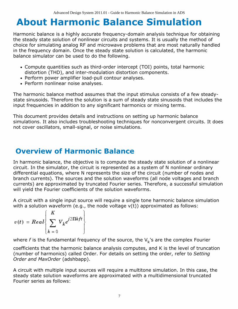
A circuit with a single input source will require a single tone harmonic balance simulationwith a solution waveform (e.g., the node voltage v(t)) approximated as follows:
where f is the fundamental frequency of the source, the Vk's are the complex Fourier
coefficients that the harmonic balance analysis computes, and K is the level of truncation(number of harmonics) called Order. For details on setting the order, refer to SettingOrder and MaxOrder (adshbapp).
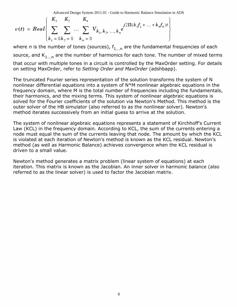
A circuit with multiple input sources will require a multitone simulation. In this case, thesteady state solution waveforms are approximated with a multidimensional truncatedFourier series as follows:
Advanced Design System 2011.01 - Guide to Harmonic Balance Simulation in ADS
8
where n is the number of tones (sources), f1...n are the fundamental frequencies of each
source, and K1...n are the number of harmonics for each tone. The number of mixed terms
that occur with multiple tones in a circuit is controlled by the MaxOrder setting. For detailson setting MaxOrder, refer to Setting Order and MaxOrder (adshbapp).
The truncated Fourier series representation of the solution transforms the system of Nnonlinear differential equations into a system of N*M nonlinear algebraic equations in thefrequency domain, where M is the total number of frequencies including the fundamentals,their harmonics, and the mixing terms. This system of nonlinear algebraic equations issolved for the Fourier coefficients of the solution via Newton's Method. This method is theouter solver of the HB simulator (also referred to as the nonlinear solver). Newton'smethod iterates successively from an initial guess to arrive at the solution.
The system of nonlinear algebraic equations represents a statement of Kirchhoff's CurrentLaw (KCL) in the frequency domain. According to KCL, the sum of the currents entering anode must equal the sum of the currents leaving that node. The amount by which the KCLis violated at each iteration of Newton's method is known as the KCL residual. Newton'smethod (as well as Harmonic Balance) achieves convergence when the KCL residual isdriven to a small value.
Newton's method generates a matrix problem (linear system of equations) at eachiteration. This matrix is known as the Jacobian. An inner solver in harmonic balance (alsoreferred to as the linear solver) is used to factor the Jacobian matrix.

Advanced Design System 2011.01 - Guide to Harmonic Balance Simulation in ADS
9
Simulation SetupThere are three main parameters to set when doing an HB simulation: Frequency, Order,MaxOrder. Additionally, two simulation setup parameters will be determined automatically(and in an optimal manner) by the simulator. These are Convergence mode and Solver. Ifconvergence is achieved and accurate results are obtained, then you don't need to gofurther. If the circuit does not converge, see Solving Convergence Problems (adshbapp).
Setting FrequencyThe Frequency parameter is found on the HB controller's Freq tab. It appears as Freq[i]on schematic, where i=1,...,number of tones (sources) in the circuit. For a single tone HBsimulation, set the Frequency to the fundamental frequency of the source used in thecircuit. For example, in a circuit with input source at 850 MHz, set Freq[1]=850 MHz.
When doing a multitone simulation, additional Frequencies need to be set on the controllercorresponding to the fundamental frequencies of the additional sources. It is stronglyrecommended to set Freq[1] to the most nonlinear tone. The most nonlinear tone istypically the one with the largest power. For example, consider a two tone HB analysis todetermine mixer conversion gain with an LO source at 1850 MHz, and an RF source at 2.1GHz. Since the LO is the more nonlinear tone, it should be set to be the first fundamental,i.e., Freq[1]=1850 MHz, while the RF should be set to Freq[2]=2.1 GHz. Next consider amixer intermodulation distortion analysis (same LO at 1850 MHz and RF at 2100 MHz). Inthis case, use a VAR component to define FrqSpacing=100k, and set the HB controllerwith Freq[1]=L0, Freq[2]=RF+FrqSpacing/2, Freq[3]=RF-FrqSpacing/2. An example ofthese circuits and simulations can be seen in Harmonic Balance for Mixers (cktsimhb).
If the frequency of the input source is not the fundamental or a related harmonic of aFrequency parameter on the controller, then the frequency of the input source is not usedin computing the steady state solution. For example, in a circuit with three sources (1GHz, 900 MHz, and 940 MHz) in which only two of the three are specified on the HBcontroller (1 GHz and 900 MHz), the third source is turned off. When this occurs, thefollowing warning message is generated:
Warning detected by HPEESOFSIM during HB analysis `HB1'. For source `SRC1',
(1xfreq[3])=9.4e+08 is 4e+07 Hz away from the closest analysis frequency at
9e+08. The maximum frequency difference for analysis time step is 900 Hz.
This spectral component is turned off for this simulation.
Setting Order and MaxOrderThe Order parameter is found on the Freq tab, and it determines the number ofharmonics used in the truncated Fourier series representation of the HB solution. TheOrder and Frequency parameters are set at the same time. The default value for Order is3. For a single tone simulation, set the Order to the desired level of Fourier seriestruncation. The Order needs to be sufficiently large so that the HB simulator can compute

Advanced Design System 2011.01 - Guide to Harmonic Balance Simulation in ADS
10
its solution waveforms to an adequate degree of accuracy. For example, in the circuit withinput source at 850 MHz and Order set to 3, the following three harmonics will be used inHB: 850 MHz, 1700 MHz, and 2550 MHz. However, three harmonics are sufficient only formostly linear circuits generating sinusoidal-like signals. For mildly nonlinear circuits, theOrder should be set to 7 or more. Highly nonlinear circuits with waveforms containingsharp edges and spikes will require many more harmonics (sometimes in the hundreds).
For multitone simulations, the Order needs to be specified for each tone. It isrecommended to use a higher Order for the more nonlinear tones. For example, in theabove mixer example, the Order for the LO tone should be at least 7, while the RF Ordercan be left at 3.
The parameter Maximum mixing order (MaxOrder on schematic), also found on theFreq tab, determines how many mixing products are to be included in a multitonesimulation. A mixing term, or mixing product, is a combination of two or morefundamentals or their successive harmonics. Mixing products will occur when there aremultiple sources in a circuit. Since the number of mixing terms can grow very large, it islimited in ADS by the following:
where kj is the harmonic for the jth tone in the circuit. The Maximum mixing order can be
set when there are two or more frequencies in the simulation. This parameter does notaffect a single tone simulation, and is therefore disabled on the Freq tab. The table belowgives a specific example with the first fundamental at 1.9 GHz with Order[1]=K1 =4, the
second fundamental at 2.1 GHz with Order[2]=K2 =5, and Maximum mixing order=3. The
DC term is always included as one of the simulation frequencies; however, it is not listedin the table.
Source Frequency Order Non-Mixed Simulation Frequencies
Fund1 (f1) 1.9 GHz 4 f1=1.9GHz, 2f1=3.8GHz, 3f1=5.7GHz, 4f1=7.6GHz
Fund2 (f2) 2.1 GHz 5 f2=2.1GHz, 2f2=4.2GHz, 3f2=6.3GHz, 4f2=8.4GHz, 5f2=10.5GHz
Order Mixing Term Frequency Maximum Mixing Order
2 f1+f2 4.0 GHz 3
2 f1-f2 0.2 GHz 3
3 2f1+f2 5.9 GHz 3
3 f1+2f2 6.1 GHz 3
3 f1-2f2 2.3 GHz 3
3 2f1-f2 1.7 GHz 3
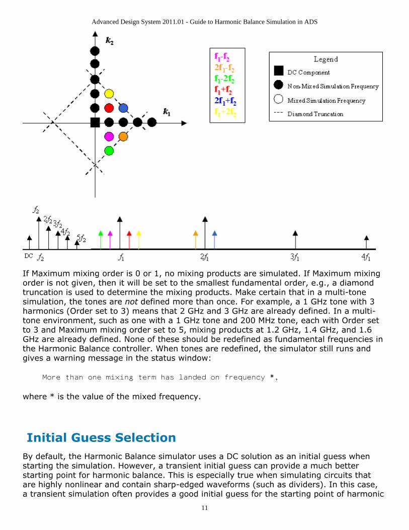
This can also be represented in a plot of k2 vs. k1. Consider the same two-tone case as
above with K1 =4 and K2 =5, and Maximum mixing order=3. The HB simulator uses a
diamond truncation method to determine which spectral components it will retain and usefor simulation. This can be seen in the following figure. Note that all of the points in theplot of k2 vs. k1 will be used in the simulation for those particular values of Order and
Maximum mixing order. The dashed lines are there to emphasize the diamond shape.
Advanced Design System 2011.01 - Guide to Harmonic Balance Simulation in ADS
11
If Maximum mixing order is 0 or 1, no mixing products are simulated. If Maximum mixingorder is not given, then it will be set to the smallest fundamental order, e.g., a diamondtruncation is used to determine the mixing products. Make certain that in a multi-tonesimulation, the tones are not defined more than once. For example, a 1 GHz tone with 3harmonics (Order set to 3) means that 2 GHz and 3 GHz are already defined. In a multi-tone environment, such as one with a 1 GHz tone and 200 MHz tone, each with Order setto 3 and Maximum mixing order set to 5, mixing products at 1.2 GHz, 1.4 GHz, and 1.6GHz are already defined. None of these should be redefined as fundamental frequencies inthe Harmonic Balance controller. When tones are redefined, the simulator still runs andgives a warning message in the status window:
More than one mixing term has landed on frequency *,
where * is the value of the mixed frequency.
Initial Guess SelectionBy default, the Harmonic Balance simulator uses a DC solution as an initial guess whenstarting the simulation. However, a transient initial guess can provide a much betterstarting point for harmonic balance. This is especially true when simulating circuits thatare highly nonlinear and contain sharp-edged waveforms (such as dividers). In this case,a transient simulation often provides a good initial guess for the starting point of harmonic
Advanced Design System 2011.01 - Guide to Harmonic Balance Simulation in ADS
12
balance. It is recommended to use a transient initial guess when simulating frequencydividers.
Automated TAHB
Transient assisted harmonic balance is automated and will be used if the simulator detectsa divider in the circuit. By default, if the simulator does not detect a divider, then it willnot use TAHB. It can also be turned on or off from the Initial Guess tab on the HarmonicBalance simulation controller. In this case, select the box labeled On, and the simulatorwill generate its own transient initial guess. The transient simulator will use intelligentdefaults and determine a steady state solution as the initial guess for harmonic balance. Itis not required to set any of the transient parameters on the Initial Guess tab. However,you may set the transient parameters only when TAHB is set to On. In that case, thesettings can be activated from the Advanced Transient Settings dialog. Transient assistedharmonic balance can be turned off by selecting Off on the Initial Guess tab. For moredetails on setting the additional transient parameters, see Transient Assisted HarmonicBalance - TAHB (adshbapp).
Advanced Design System 2011.01 - Guide to Harmonic Balance Simulation in ADS
13
Solving Convergence ProblemsThis section discusses the different types of convergence problems that can occur whenusing the Harmonic Balance simulator. It also includes the remedies for these possibleconvergence problems. The parameters used for convergence are mentioned in thissection, and are thoroughly described in Additional Parameters (adshbapp).
Prior to fixing a convergence problem, you should have some familiarity with theConvergence mode and Solver type parameters. Realize that the nonlinear outer solver,Newton solver, and Convergence mode parameter are one in the same. Similarly, thelinear solver, inner solver, and solver type are one in the same. By default, theseparameters are automatically adjusted by the simulator to achieve both speed androbustness. Convergence mode and Solver type are found on the Solver tab of the HBcontroller. Although it is not recommended to modify the Convergence mode or Solvertype, you have the option to do so.
Convergence ModeThere are three choices for the nonlinear (outer) solver that can be selected by setting the Convergence mode (ConvMode on schematic). The maximum number of iterations forthe nonlinear solver is controlled by the parameter Max. Iterations (MaxIters onschematic). Max Iterations can be set to Fast, Robust, or a Custom value. TheConvergence mode parameter options are described below.
Auto This is the default mode setting. It is both fast and robust. This mode willautomatically activate advanced features to achieve convergence. The auto modealso allows for convergence at looser tolerances if the simulation does not meet thedefault tolerances. A warning message appears in the status window when thisoccurs, and it includes the tolerance level up to which convergence was achieved.Robust This option enables an advanced Newton solver. This mode is extremelyrobust, and ensures maximal KCL residual reduction at each iteration. The Robustconvergence mode usually simulates slightly slower, yet works well for very nonlinearcircuits (i.e., those with very high power levels). It is recommended that themaximum number of iterations (MaxIters) be set to Robust when this mode isselected. Another option is to select Custom and enter a value of 50 or higher.Fast This option enables the basic Newton solver. It is fast and performs well formost circuits. For highly nonlinear circuits, this mode may have difficultiesconverging. It is then recommended to switch to the Robust convergence mode.
Solver TypeWhen using harmonic balance, you can allow the simulator to choose a solverautomatically, or select one of two linear (inner) solver techniques: Direct or Krylov. Thelinear solver is used to solve the matrix problem generated at each iteration of the Newton(outer) solver. The matrix size will be determined by both the size of the circuit and the

Advanced Design System 2011.01 - Guide to Harmonic Balance Simulation in ADS
14
total number of frequencies (fundamentals, their harmonics, and mixing products).
Auto Select Solver
This option allows the simulator to choose which solver to use. The Auto select solver isenabled by default. The simulator analyzes factors such as circuit or spectral complexityand compares memory requirements for each solver against the available computermemory. Based on this analysis it selects either the Direct or Krylov solver in a mannertransparent to you. The selection choice heavily depends upon the amount of availableRAM. The simulator will determine roughly how much RAM is available. Alternately, youcan specify the amount of RAM to allocate; however, if this is not enough for thesimulator, then it will either allocate more RAM or report an error. Furthermore, if theKrylov solver is chosen by the simulator, several options for that solver also are setautomatically.
It is possible to override the choice of solver given by the Auto select solver option. Thiscan be done simply by selecting Direct or Krylov from the Solver tab on the HB controller.When simulating large circuits, that is, those with many devices and harmonics, it isrecommended to use the Krylov solver.
Direct Solver
The Direct solver uses direct matrix factoring methods (such as Gaussian elimination) toinvert the Jacobian matrix. This solver is recommended for small circuits with relativelyfew devices, non-linear components, and number of harmonics. For large circuits, thedirect solver will be slow and inefficient. This is because the computation time of the directsolver grows with the cube of the matrix size. For example, in a single-tone HB simulation,doubling the circuit size or doubling the number of harmonics (the Order) will slow thesimulation run time by a factor of 8. Also, since the direct solver requires an explicitstorage of the Jacobian, its memory requirements grow with the square of the matrix size.For example, the factorization of a Jacobian with a size 500 will require 2500 times asmuch RAM as one with a size of 10.
Krylov Solver
An alternate approach to solving the matrix problem is to use a Krylov subspace iterativemethod such as GMRES. The Krylov method is intended for solving large circuits withmany devices, non-linear components, and number of harmonics. (A large circuit can beroughly described as one in which a simulation using the direct solver exceeds 100 MB ofmemory usage or the memory capacity of the computer, whichever occurs first.) TheKrylov solver does not require the explicit storage of the Jacobian matrix, but rather onlythe ability to carry out matrix-vector products. As a result, Krylov solver's memoryrequirements grow linearly with the matrix size, rather than quadratically as in the directmethod. Thus, Krylov solvers offer substantial memory usage savings for large circuit
Advanced Design System 2011.01 - Guide to Harmonic Balance Simulation in ADS
15
problems. Since the Krylov method solves the matrix problem to a loose tolerance, it isalso much faster than the direct solver (but less robust). The computation time of theKrylov solver grows slightly faster than linear with the matrix size. For example, doublingthe circuit size or doubling the number of harmonics will increase the simulation run timeby slightly more than a factor of 2.
Setting Status Level and Understanding Output in theStatus WindowDuring an HB simulation, the simulator prints information describing the simulationprogress in the status server window. The Status level parameter (found on the Freqtab) controls the amount of detail in this information. Reading and understanding thisinformation is critical to solving convergence problems.
The default status level is set to 2; however, when solving a convergence problem, it isbest to set the status level to 4. For each Newton iteration the L-1 norm of the KCLresiduals throughout the circuit is printed.
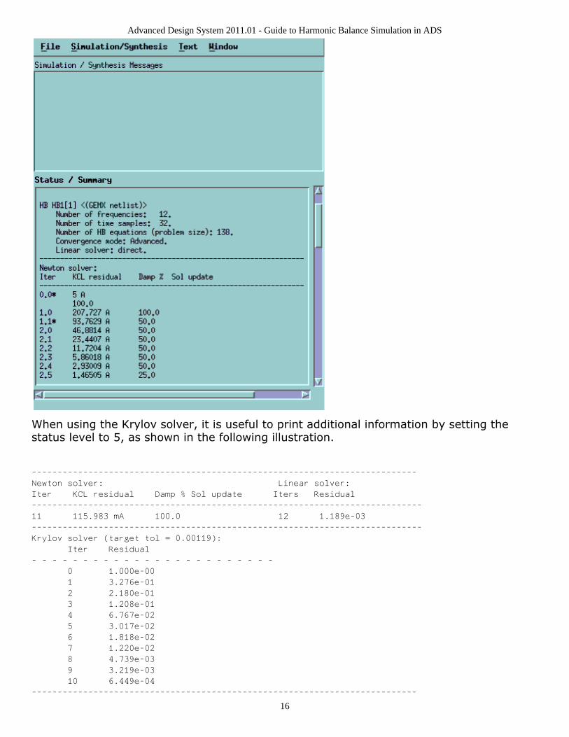
The KCL residual indicates how well the circuit has converged up to that point. A steadilydecreasing residual implies successful convergence. For example, for an HB simulation atdefault (strict) tolerances, this residual should reach levels of pico amps at the end. Asnap shot of the ADS Status Server Window is shown in the following figure.
Advanced Design System 2011.01 - Guide to Harmonic Balance Simulation in ADS
16
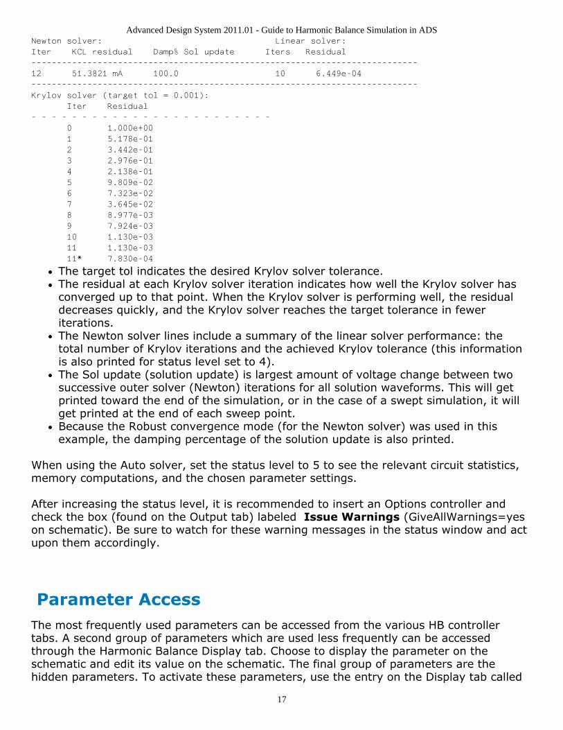
When using the Krylov solver, it is useful to print additional information by setting thestatus level to 5, as shown in the following illustration.
---------------------------------------------------------------------------
Newton solver: Linear solver:
Iter KCL residual Damp % Sol update Iters Residual
----------------------------------------------------------------------------
11 115.983 mA 100.0 12 1.189e-03
----------------------------------------------------------------------------
Krylov solver (target tol = 0.00119):
Iter Residual
- - - - - - - - - - - - - - - - - - - - - - - -
0 1.000e-00
1 3.276e-01
2 2.180e-01
3 1.208e-01
4 6.767e-02
5 3.017e-02
6 1.818e-02
7 1.220e-02
8 4.739e-03
9 3.219e-03
10 6.449e-04
---------------------------------------------------------------------------
Advanced Design System 2011.01 - Guide to Harmonic Balance Simulation in ADS
17
Newton solver: Linear solver:
Iter KCL residual Damp% Sol update Iters Residual
----------------------------------------------------------------------------
12 51.3821 mA 100.0 10 6.449e-04
----------------------------------------------------------------------------
Krylov solver (target tol = 0.001):
Iter Residual
- - - - - - - - - - - - - - - - - - - - - - - -
0 1.000e+00
1 5.178e-01
2 3.442e-01
3 2.976e-01
4 2.138e-01
5 9.809e-02
6 7.323e-02
7 3.645e-02
8 8.977e-03
9 7.924e-03
10 1.130e-03
11 1.130e-03
11* 7.830e-04
The target tol indicates the desired Krylov solver tolerance.The residual at each Krylov solver iteration indicates how well the Krylov solver hasconverged up to that point. When the Krylov solver is performing well, the residualdecreases quickly, and the Krylov solver reaches the target tolerance in feweriterations.The Newton solver lines include a summary of the linear solver performance: thetotal number of Krylov iterations and the achieved Krylov tolerance (this informationis also printed for status level set to 4).The Sol update (solution update) is largest amount of voltage change between twosuccessive outer solver (Newton) iterations for all solution waveforms. This will getprinted toward the end of the simulation, or in the case of a swept simulation, it willget printed at the end of each sweep point.Because the Robust convergence mode (for the Newton solver) was used in thisexample, the damping percentage of the solution update is also printed.
When using the Auto solver, set the status level to 5 to see the relevant circuit statistics,memory computations, and the chosen parameter settings.
After increasing the status level, it is recommended to insert an Options controller andcheck the box (found on the Output tab) labeled Issue Warnings (GiveAllWarnings=yeson schematic). Be sure to watch for these warning messages in the status window and actupon them accordingly.
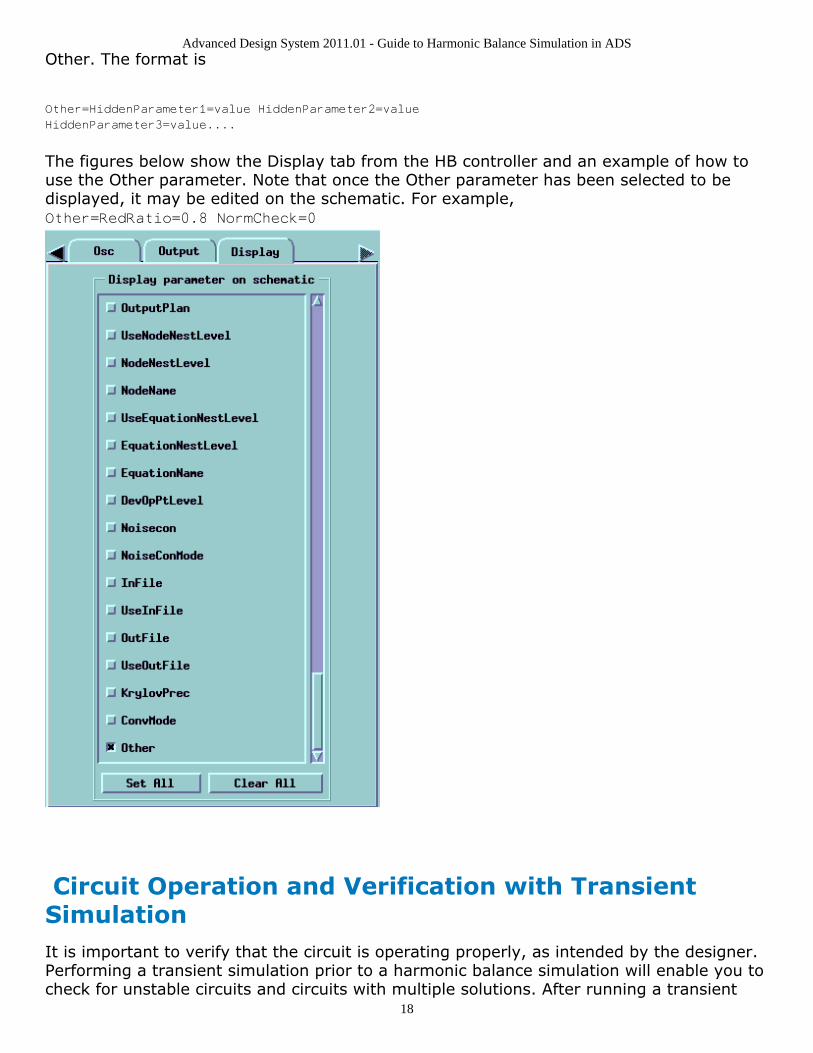
Parameter AccessThe most frequently used parameters can be accessed from the various HB controllertabs. A second group of parameters which are used less frequently can be accessedthrough the Harmonic Balance Display tab. Choose to display the parameter on theschematic and edit its value on the schematic. The final group of parameters are thehidden parameters. To activate these parameters, use the entry on the Display tab called
Advanced Design System 2011.01 - Guide to Harmonic Balance Simulation in ADS
18
Other. The format is
Other=HiddenParameter1=value HiddenParameter2=value
HiddenParameter3=value....
The figures below show the Display tab from the HB controller and an example of how touse the Other parameter. Note that once the Other parameter has been selected to bedisplayed, it may be edited on the schematic. For example,Other=RedRatio=0.8 NormCheck=0
Circuit Operation and Verification with TransientSimulationIt is important to verify that the circuit is operating properly, as intended by the designer.Performing a transient simulation prior to a harmonic balance simulation will enable you tocheck for unstable circuits and circuits with multiple solutions. After running a transient
Advanced Design System 2011.01 - Guide to Harmonic Balance Simulation in ADS
19
analysis, check to see if the waveforms blow up or have several spikes and sharp edges.In the case that the waveforms have these conditions, Harmonic Balance may requirehundreds or even thousands of harmonics which in turn will significantly increasesimulation run time and memory usage.
Harmonic Balance Controller SetupWhen a circuit does not converge, it is important to check that the controller is set upcorrectly and with appropriate controller parameter settings.
Order
The Harmonic Balance solution is approximated by a truncated Fourier series. Whenconvergence problems begin to occur, the first parameter to examine is the Order, whichis the number of harmonics. The lower the Order, the greater the error due to Fouriertruncation in the solution representation. The Order needs to be sufficiently large torepresent nonlinear signals such as those with sharp transitions or square waves. Ifincreasing the order causes the simulation speed to dramatically slow down or there is anexcessive usage of memory, then it is best to switch from the direct solver to using theKrylov solver.
By setting the status level to 4 or more, an HB truncation error warning may be given inthe status window upon a successful completion of an HB simulation. The warningcontains a sorted table of the five waveforms in violation of the HB truncation error checkwith largest HB truncation errors. Note that the HB truncation error check is not the sameas the circuit convergence check for the KCL residual; in fact, the HB truncation errorwarning can be generated only once the circuit has converged. The HB truncation errormay not be distributed evenly across all of the computed harmonics.
If fewer than five waveforms violate the HB truncation error check, only those will beprinted. If there are no violating waveforms, then the HB truncation error warning is notprinted at all. Increasing the order will reduce the number of violating waveforms. Anexample of the warning message for HB truncation error is shown below:
Warning detected by HPEESOFSIM during HB analysis `HB1'.
An HB truncation error may be present.
o The HB truncation error is due to using a finite order
(number of harmonics) in the representation of the
circuit signals.
Waveform Trunc error Tolerance
---------------------------------------------------------
v2 6.576e-03 > 5.941e-06
v3 1.780e-03 > 1.043e-06
o Number of waveforms violating the HB truncation error check:
2 out of 2 waveforms.
o Estimated max HB truncation error: 6.576e-03 @ waveform v2.
o The maximal HB truncation error estimate is greater than the
Advanced Design System 2011.01 - Guide to Harmonic Balance Simulation in ADS
20
achieved tolerance of 5.941e-06 for this waveform.
o A time-domain plot of the v3 waveform may show the error as
Gibbs ripples.
o To reduce the error, increase the order (number of harmonics)
and re-simulate.
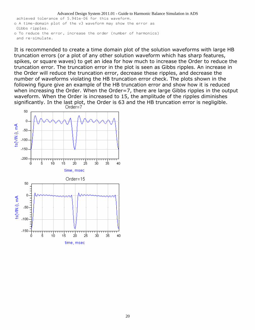
It is recommended to create a time domain plot of the solution waveforms with large HBtruncation errors (or a plot of any other solution waveform which has sharp features,spikes, or square waves) to get an idea for how much to increase the Order to reduce thetruncation error. The truncation error in the plot is seen as Gibbs ripples. An increase inthe Order will reduce the truncation error, decrease these ripples, and decrease thenumber of waveforms violating the HB truncation error check. The plots shown in thefollowing figure give an example of the HB truncation error and show how it is reducedwhen increasing the Order. When the Order=7, there are large Gibbs ripples in the outputwaveform. When the Order is increased to 15, the amplitude of the ripples diminishessignificantly. In the last plot, the Order is 63 and the HB truncation error is negligible.
Advanced Design System 2011.01 - Guide to Harmonic Balance Simulation in ADS
21
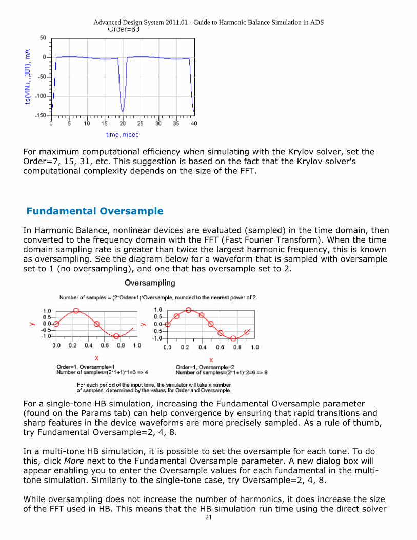
For maximum computational efficiency when simulating with the Krylov solver, set theOrder=7, 15, 31, etc. This suggestion is based on the fact that the Krylov solver'scomputational complexity depends on the size of the FFT.
Fundamental Oversample
In Harmonic Balance, nonlinear devices are evaluated (sampled) in the time domain, thenconverted to the frequency domain with the FFT (Fast Fourier Transform). When the timedomain sampling rate is greater than twice the largest harmonic frequency, this is knownas oversampling. See the diagram below for a waveform that is sampled with oversampleset to 1 (no oversampling), and one that has oversample set to 2.
For a single-tone HB simulation, increasing the Fundamental Oversample parameter(found on the Params tab) can help convergence by ensuring that rapid transitions andsharp features in the device waveforms are more precisely sampled. As a rule of thumb,try Fundamental Oversample=2, 4, 8.
In a multi-tone HB simulation, it is possible to set the oversample for each tone. To dothis, click More next to the Fundamental Oversample parameter. A new dialog box willappear enabling you to enter the Oversample values for each fundamental in the multi-tone simulation. Similarly to the single-tone case, try Oversample=2, 4, 8.
While oversampling does not increase the number of harmonics, it does increase the sizeof the FFT used in HB. This means that the HB simulation run time using the direct solver
Advanced Design System 2011.01 - Guide to Harmonic Balance Simulation in ADS
22
(which is determined by the Order and the circuit size) is not largely affected when theFundamental Oversample is increased. However an HB simulation run time using theKrylov solver will be slower since this solver's computational complexity depends on thesize of the FFT.
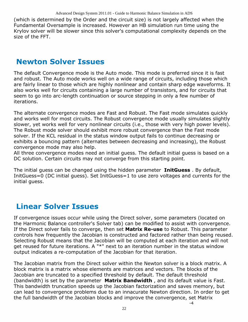
Newton Solver IssuesThe default Convergence mode is the Auto mode. This mode is preferred since it is fastand robust. The Auto mode works well on a wide range of circuits, including those whichare fairly linear to those which are highly nonlinear and contain sharp edge waveforms. Italso works well for circuits containing a large number of transistors, and for circuits thatseem to go into arc-length continuation or source stepping in only a few number ofiterations.
The alternate convergence modes are Fast and Robust. The Fast mode simulates quicklyand works well for most circuits. The Robust convergence mode usually simulates slightlyslower, yet works well for very nonlinear circuits (i.e., those with very high power levels).The Robust mode solver should exhibit more robust convergence than the Fast modesolver. If the KCL residual in the status window output fails to continue decreasing orexhibits a bouncing pattern (alternates between decreasing and increasing), the Robustconvergence mode may also help.All three convergence modes need an initial guess. The default initial guess is based on aDC solution. Certain circuits may not converge from this starting point.
The initial guess can be changed using the hidden parameter InitGuess . By default,InitGuess=0 (DC initial guess). Set InitGuess=1 to use zero voltages and currents for theinitial guess.
Linear Solver IssuesIf convergence issues occur while using the Direct solver, some parameters (located onthe Harmonic Balance controller's Solver tab) can be modified to assist with convergence.If the Direct solver fails to converge, then set Matrix Re-use to Robust. This parametercontrols how frequently the Jacobian is constructed and factored rather than being reused.Selecting Robust means that the Jacobian will be computed at each iteration and will notget reused for future iterations. A "*" next to an iteration number in the status windowoutput indicates a re-computation of the Jacobian for that iteration.
The Jacobian matrix from the Direct solver within the Newton solver is a block matrix. Ablock matrix is a matrix whose elements are matrices and vectors. The blocks of theJacobian are truncated to a specified threshold by default. The default threshold(bandwidth) is set by the parameter Matrix Bandwidth , and its default value is Fast.This bandwidth truncation speeds up the Jacobian factorization and saves memory, butcan lead to convergence problems due to an innacurate Newton direction. In order to getthe full bandwidth of the Jacobian blocks and improve the convergence, set Matrix
-4
Advanced Design System 2011.01 - Guide to Harmonic Balance Simulation in ADS
23
Bandwidth to Robust. Typical values for the Custom entry range from 10 to 0.
If convergence issues occur while using the Krylov solver, increase the status level to 5and monitor the KCL residual and the Krylov solver residual in the status window. If theKrylov solver converges very slowly, its iterations may be terminated before the linearproblem can be solved to an acceptable degree of accuracy. In such a case, the followingmessage will appear in the status window output:
<name_of_Krylov_solver> terminating due to insufficient rate of convergence.
It is recommended to set the Krylov Restart Length (GMRES_Restart on schematic)parameter to Custom and enter a value between 10 and 100. The default setting isRobust. However, if there is a limited amount of memory available, then select LowMemory. This parameter determines the number of iterations after which the Krylov solveris restarted. Also, to prevent the Krylov solver from stopping too soon due to "insufficientrate of convergence", increase the Krylov Convergence Ratio (KrylovConvRatio onschematic). This is the amount by which the norm of the Krylov solution must decreasefrom one iteration to the next. The default is 0.9 and it should not be larger than 1.0.
As a last resort, it is recommended to change the Krylov preconditioner. A preconditioner is used to increase the rate of convergence of the Krylov linear solver byreducing the number of iterations performed. Thus, preconditioning is essential to makingthe Krylov solver effective. Click Advanced Krylov Parameters to choose thepreconditioner.
The default preconditioner is DCP. Some of the Krylov solver's convergence problems arisedue to the limitations of the DCP. There can be multiple reasons for these problems, suchas strong nonlinearities in the circuit generating an ill-conditioned linear problem at eachNewton iteration. As a result the Newton direction becomes inaccurate so that thenonlinear solver fails to converge. When the Krylov solver has trouble converging, it isrecommended to change the preconditioner to BSP or SCP. The BSP typically is moreefficient for medium to large size problems, while SCP works better for very largeproblems. Changing the preconditioner should be done only when an error messageappears in the status window giving specific instructions to change the preconditioner.
The three types of preconditioners used by the simulator are summarized below. You mustselect one when using the Krylov solver:
DC Preconditioner (DCP) This is the default preconditioner, which is effective inmost cases, but fails for some highly non-linear circuits. It uses a DC approximationon the entire circuit.Block Select Preconditioner (BSP) This is recommended for instances when aKrylov HB simulation fails to converge using the DCP option. The BSP preconditioneris more robust than the DCP for highly nonlinear circuits. For the circuits thatconverge with DCP, the overhead introduced by the BSP preconditioner is small. Forcircuits that fail with the DCP, using the BSP option often achieves convergence atthe cost of additional memory usage.Schur-Complement Preconditioner (SCP) This is also intended for use withcircuits that fail to converge with the DCP preconditioner. This is a robust choice forhighly nonlinear circuits. It uses the DC approximation for most of the circuit similar
Advanced Design System 2011.01 - Guide to Harmonic Balance Simulation in ADS
24
to DCP. The most nonlinear parts of the circuit are excluded and are instead factoredwith a specialized Krylov solver known as DMRES. The complex technology of the SCPpreconditioner results in a memory usage overhead. This overhead is due toconstruction of a knowledge base enabling the SCP to be much more efficient in thelater use of the harmonic balance solution process.
Sweeps as Convergence ToolsParameter sweeps can be used to formulate a customized continuation method gearedtoward the particular circuit problem. Continuation methods provide a sequence of initialguesses that generate a sequence of solutions that approach the final desired solution.
There are two main ways to perform a parameter sweep in ADS. The first way is to usethe Sweep tab within the HB controller. This is the most efficient way to perform sweeps,and thus is the preferred way. The second way is to include a Parameter Sweep controller,which is a separate controller from the HB controller. For single parameter sweeps (inwhich the swept parameter is not frequency), use the Sweep tab on the HB controller. Formulti-dimensional sweeps, use the Sweep tab for the inner-most sweep parameter, anduse the Parameter Sweep controller(s) for the outer-most sweep parameter(s). Frequencyshould always be selected as an outer-most sweep parameter even for multi-tonesimulations.
When a single point HB simulation does not converge, a parameter sweep can be used asa convergence tool. Performing a sweep around a single point that does not convergehelps to determine if there is a range of values for which the circuit can converge.Selecting which parameter to sweep is the first step. It is best to choose a parameter thatcan be set to a value for which the circuit will easily converge. Some examples are thesource amplitude or power, a bias voltage or current, or any component parameter thatcontrols the amount of nonlinearity in the circuit. Find the parameter value for which thecircuit converges and make this the start point of the sweep. The actual parameter valuefor which the circuit does not converge should be the end point of the sweep. Perform aswept simulation up to the point for which the circuit converges, and save the solution tobe used as an initial guess for single point simulation that does not converge. Simulate thesingle point with this initial guess. This may give the Newton solver a better initial guessthan the DC solution.
In most cases, a linear sweep will work best. When performing a sweep, be sure that theRegenerate Initial Guess for Param Sweep (Restart) is not checked (i.e., Restart=no). Thisensures that the sweep will be used as a continuation, or in other words, the solution fromthe previous sweep step is used as an initial guess for the next step. Having more sweeppoints will give a greater chance for success, but will result in a longer computation time.
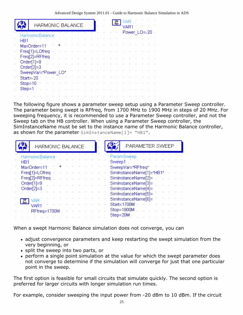
Two diagrams are shown, one for each sweep method. The following figure shows theHarmonic Balance controller sweeping the variable Power_LO from -20 dbm to 10 dBm insteps of 1 dBm. A VAR equation needs to be included to initialize the parameter that is tobe swept. The value of this parameter in the VAR equation can be set to an arbitrarynumber, since the value of the sweep start will override this value.
Advanced Design System 2011.01 - Guide to Harmonic Balance Simulation in ADS
25
The following figure shows a parameter sweep setup using a Parameter Sweep controller.The parameter being swept is RFfreq, from 1700 MHz to 1900 MHz in steps of 20 MHz. Forsweeping frequency, it is recommended to use a Parameter Sweep controller, and not theSweep tab on the HB controller. When using a Parameter Sweep controller, theSimInstanceName must be set to the instance name of the Harmonic Balance controller,as shown for the parameter SimInstanceName[1]= "HB1".
When a swept Harmonic Balance simulation does not converge, you can
adjust convergence parameters and keep restarting the swept simulation from thevery beginning, orsplit the sweep into two parts, orperform a single point simulation at the value for which the swept parameter doesnot converge to determine if the simulation will converge for just that one particularpoint in the sweep.
The first option is feasible for small circuits that simulate quickly. The second option ispreferred for larger circuits with longer simulation run times.
For example, consider sweeping the input power from -20 dBm to 10 dBm. If the circuit
Advanced Design System 2011.01 - Guide to Harmonic Balance Simulation in ADS
26
does not converge, reduce the range of the sweep so that the last point is the one forwhich the circuit will still converge (this is the first sweep). Suppose the circuit convergedonly up to 5 dBm. The 5 dBm solution can be saved in an output file: select theparameters Write Final Solution and enter the name of the file for the output to be saved.Adjust parameters such as Order, Oversample, and number of iterations; then try asecond sweep from 5 to 10 dBm and see if the circuit will go beyond 5 dBm. The 5 dBmoutput file should be used as an initial guess for this second sweep: select Use InitialGuess and enter the name of the file.
As a more detailed example, consider sweeping the RF frequency in a mixer circuit (withthe Fast convergence mode and Krylov solver) from 0.5 GHz to 1.5 GHz, using 11 sweeppoints (0.1 GHz step size). Suppose this circuit can only converge up to the RF frequencypoint of 1.0 GHz and fails at 1.1 GHz. At this point, it is recommended to follow thesesteps:
Break the sweep into two parts (the first part will be a sweep over the range of1.frequencies for which the circuit converges, and the second part will be the remainingsweep points).Simulate the first part to generate an initial guess which can be used for the second2.sweep.Adjust parameters to achieve convergence for the second part of the sweep.3.
For this mixer example, it is desired to have 11 sweep points between 0.5 GHz and 1.5GHz. This means that spacing between sweep points is (1.0 GHz)/10 = 0.1 GHz. Thefrequency sweep points are then placed at: 500 MHz, 600 MHz, 700 MHz, 800 MHz, 900MHz, 1000 MHz, 1100 MHz, 1200 MHz, 1300 MHz, 1400 MHz, and 1500 MHz. Setup thesimulation for the first sweep with a VAR block to define fstart1=0.5G, fstep1=1.0G/10,fstop1=fstart+5*fstep, and np1=6. Since the simulation does not converge beyond 1 GHz,the first sweep is done up to that point, which is 5 frequency points after the start i.e.,fstop1=fstart+5*fstep. The total number of points for the first sweep is 6 (np1=6). Theremaining 5 points will be used for the second half of the sweep.
Instantiate a Parameter Sweep controller, and set Start=fstart1, Stop=fstop1, and Num.of Points=np1. The sweep step size will be determined by the Num. of Points, and will beequivalent to the value for fstep. It is not necessary to specify the step size parameterwhen specifying the Num. of Points parameter. Next, on the Harmonic Balance controller'sParams tab, select Write Final Solution and enter the name of the file that will be used asan initial guess for the second sweep. Run the HB simulation. After it completes, add thefollowing equations to the VAR block - fstart2=fstop1+fstep1, fstop2=1.5G, np2=5. Wewant the second sweep to start from the point at which the original sweep failed, thus,fstart2=fstop1+fstep1. There are five remaining points, so np2=5. Go back to the HBcontroller, and on the Initial Guess tab, unselect Write Final Solution. Now select UseInitial Guess and enter the name of the file that was written during the first sweep. Next,return to the Parameter Sweep controller, set Start=fstart2, Stop=fstop2, and Num. OfPoints=np2. (Or deactivate the Parameter Sweep controller and instantiate a new one withthe sweep var as RFfreq but with the start and stop with the values for the secondsweep). It is not necessary to enter the step size since that is determined by using theNum. Of Points, and the Start and Stop. The next step is to adjust certain parameters toachieve convergence. Recall that the nonconverging simulation was using the Fastconvergence mode. For the second half of the sweep, it is then recommended to use the
Advanced Design System 2011.01 - Guide to Harmonic Balance Simulation in ADS
27
Robust convergence mode (found on the Solver tab) with the Krylov solver. For this mixercircuit, convergence was achieved using the Robust mode. Alternatively, the entire sweepcould have been performed using the Robust convergence mode from the beginning ratherthan performing two sweeps. However, this approach is less efficient than the two partsweep due to the overhead computation required by the Robust mode in the first part ofthe sweep.
NoteAfter doing a HB analysis, you may want to do an HB noise analysis. A saved final solution may be used asthe initial guess for other simulations such as noise analysis (of the same circuit) so that the nodevoltages and branch currents do not have to be recalculated.
Transient Assisted Harmonic Balance - TAHB The DC solution is the default initial guess; however, a transient solution can be a betterinitial guess for the Newton solver. The size of the initial KCL residual (seen from thestatus window output) is a measure of the quality of the initial guess (the smaller the KCLresidual, the better the initial guess). A better initial guess such as TAHB can yield severalorders of magnitude improvement in the initial KCL residual. For circuits that are highlynonlinear and contain sharp-edged waveforms (such as dividers), a transient simulationoften provides a good initial guess for the starting point of harmonic balance.
Automated TAHB
By default, the HB simulator will determine if there is a divider in the circuit. If so, atransient simulation will be performed to create an initial guess for the HB simulation.TAHB can also be turned on or off from the Initial Guess tab by selecting On or Off,respectively. When a divider is detected or if TAHB is set to On, the transient simulatorwill use intelligent defaults and determine a steady state solution as the initial guess forharmonic balance. It is not required to set any of the other parameters on the InitialGuess tab. The transient parameters can be set only when TAHB is set to On.
Setting Advanced Transient Parameters
Advanced transient parameters can be set when TAHB is set to On . Some are includedon the Initial Guess tab in the Transient Assisted Harmonic Balance section underAdvanced Transient Parameters. The first parameter is the StopTime, e.g., the endingtime for the transient simulation. The default is 100 cycles of the commensuratefrequency. (For a one tone analysis, this would be Freq[1]). If the transient simulatordetects steady state, then the simulation will end one period after that time point, andthus earlier than the StopTime. The one period after the time point gets transformed tothe frequency domain for harmonic balance. If transient does not reach steady state, thenthe last period before the StopTime will get transformed to the frequency domain, andharmonic balance will use that for the initial guess. If convergence is not achieved in this
Advanced Design System 2011.01 - Guide to Harmonic Balance Simulation in ADS
28
case, then it is recommended to increase the StopTime so that transient runs longer than100 cycles.
The second parameter is MaxTimeStep. The default is 1/(2*4*Maximum frequency). In asingle tone analysis, the maximum frequency would be Freq[1]*Order[1]. Be sure to setMaxTimeStep small enough to accommodate the largest frequency. The simulator willdisplay the values that it determined for StopTime and MaxTimeStep in the status window.
The third parameter is Min Time for detecting steady state (SteadyStateMinTime onschematic). This is the earliest point in time that the transient simulator starts checkingfor steady state conditions. The default is two periods of the fundamental frequency forautonomous circuits, and 10 periods of the fundamental frequency for non-autonomouscircuits such as an oscillator. The units for this parameter are in seconds. If your circuitexhibits a large amount of over/undershoot, then this to be larger than the default so thatthe detector will begin to check for steady state after some of the initial transients havesettled.
The fourth parameter is IV_RelTol. This is the transient current and voltage relativetolerance, and the default is 1e-3. It is specific to the transient analysis and will overridethe relative tolerances on the Options controller if one is found in the schematic. If anOptions controller is included in the schematic, be sure to set the IV_RelTol to areasonable value, such as 1e-3. Otherwise the transient simulation would run for a verylong time since it would use the relative tolerances on the Options controller which are setfor harmonic balance.
Any transient parameter that is not found on the tab can be set using the Transient Otherparameter. For example, one could set the following transient convolution parameterImpMaxFreq=10 GHz.
When TAHB is set to On, a user-supplied initial guess is not able to be specified, and thusit is not interpreted at all. If one is given and TAHB is set to Auto (the default), the user-supplied initial guess takes the highest precedence.
Using a One-Tone Transient for a Multi-Tone Harmonic Balance
An initial guess generated by a single tone transient simulation may be used for a multi-tone harmonic balance simulation. This approach is strongly recommended, and will oftenresult in much better convergence than with a multi-tone transient simulation. Theparameter Use only Freq[1] for transient instructs transient simulator to perform a onetone simulation, and to only use the value of Freq[1] on the harmonic balance controllerfor determining the StopTime and MaxTimeStep. The default is yes. If there are multiplefrequencies on the HB controller and this parameter is yes, then sources in the circuit atthe other frequencies will be turned off for the transient portion only. Also, Freq[1] shouldbe set to the frequency of the most nonlinear tone.
Swept and Optimizations Simulations with TAHB
Advanced Design System 2011.01 - Guide to Harmonic Balance Simulation in ADS
29
Any optimization or statistical analyses such as optimization, yield, Monte Carlo, DOE, andyield-optimization are not supported with automated TAHB. The simulation will use thestandard harmonic balance in those cases.
When sweeping a parameter on the sweep tab, a transient simulation is done for theharmonic balance simulation of the first sweep point only. When sweeping a parameter onthe ParamSweep controller, a transient simulation will be done for the first sweep pointonly, unless the Regenerate Initial Guess for ParamSweep (Restart) parameter is set toyes, e.g., the check box is selected. In the case that the Restart is set to yes, a transientsimulation will be done at each sweep point and thus generate a new transient initialguess for each sweep point of the harmonic balance simulation.
Divide-by-8 Example
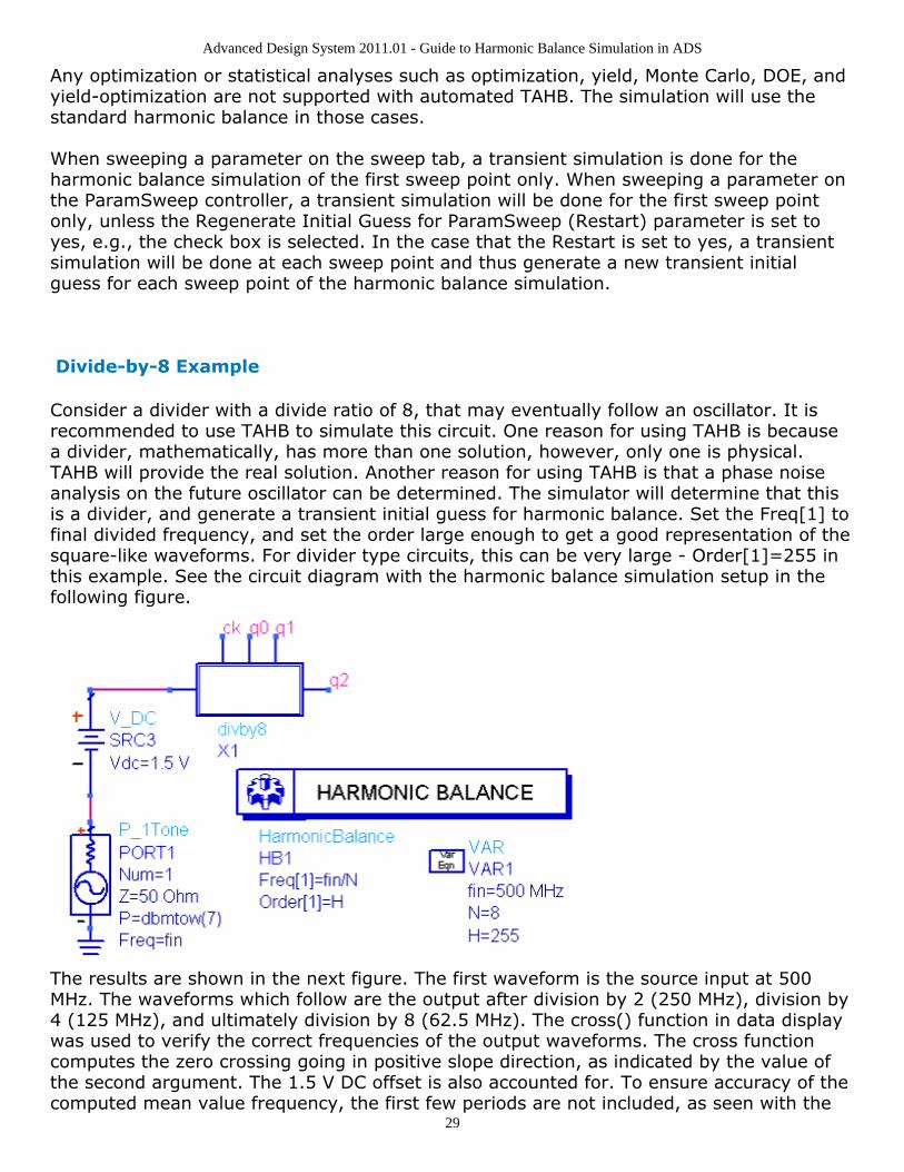
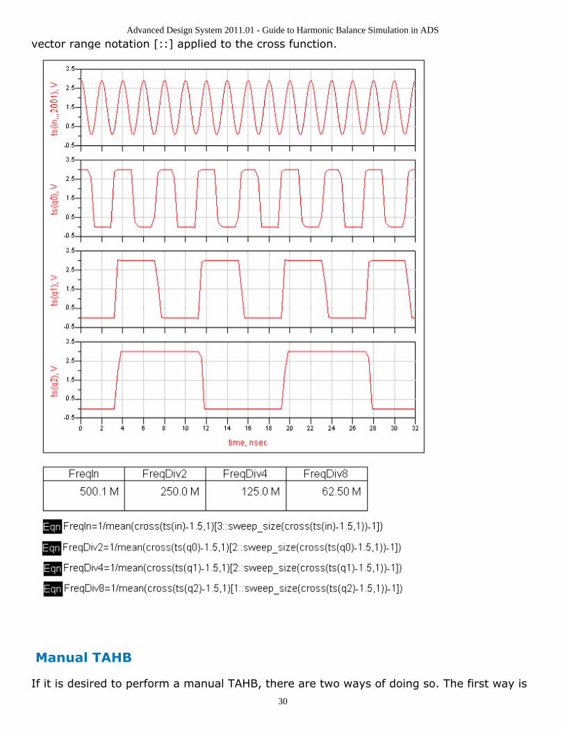
Consider a divider with a divide ratio of 8, that may eventually follow an oscillator. It isrecommended to use TAHB to simulate this circuit. One reason for using TAHB is becausea divider, mathematically, has more than one solution, however, only one is physical.TAHB will provide the real solution. Another reason for using TAHB is that a phase noiseanalysis on the future oscillator can be determined. The simulator will determine that thisis a divider, and generate a transient initial guess for harmonic balance. Set the Freq[1] tofinal divided frequency, and set the order large enough to get a good representation of thesquare-like waveforms. For divider type circuits, this can be very large - Order[1]=255 inthis example. See the circuit diagram with the harmonic balance simulation setup in thefollowing figure.
The results are shown in the next figure. The first waveform is the source input at 500MHz. The waveforms which follow are the output after division by 2 (250 MHz), division by4 (125 MHz), and ultimately division by 8 (62.5 MHz). The cross() function in data displaywas used to verify the correct frequencies of the output waveforms. The cross functioncomputes the zero crossing going in positive slope direction, as indicated by the value ofthe second argument. The 1.5 V DC offset is also accounted for. To ensure accuracy of thecomputed mean value frequency, the first few periods are not included, as seen with the
Advanced Design System 2011.01 - Guide to Harmonic Balance Simulation in ADS
30
vector range notation [::] applied to the cross function.
Manual TAHB
If it is desired to perform a manual TAHB, there are two ways of doing so. The first way is
Advanced Design System 2011.01 - Guide to Harmonic Balance Simulation in ADS
31
to use the steady state detector in transient and allow the simulator to automaticallycapture the steady state portion for the initial guess. The second way is to manuallyadjust the transient StartTime and the StopTime to capture the steady state portion of thewaveform.
Running Transient and Generating the Initial Guess
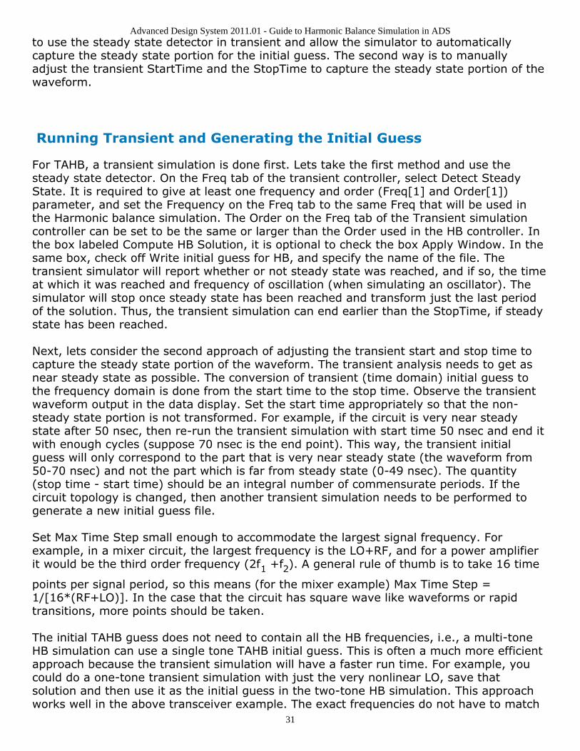
For TAHB, a transient simulation is done first. Lets take the first method and use thesteady state detector. On the Freq tab of the transient controller, select Detect SteadyState. It is required to give at least one frequency and order (Freq[1] and Order[1])parameter, and set the Frequency on the Freq tab to the same Freq that will be used inthe Harmonic balance simulation. The Order on the Freq tab of the Transient simulationcontroller can be set to be the same or larger than the Order used in the HB controller. Inthe box labeled Compute HB Solution, it is optional to check the box Apply Window. In thesame box, check off Write initial guess for HB, and specify the name of the file. Thetransient simulator will report whether or not steady state was reached, and if so, the timeat which it was reached and frequency of oscillation (when simulating an oscillator). Thesimulator will stop once steady state has been reached and transform just the last periodof the solution. Thus, the transient simulation can end earlier than the StopTime, if steadystate has been reached.
Next, lets consider the second approach of adjusting the transient start and stop time tocapture the steady state portion of the waveform. The transient analysis needs to get asnear steady state as possible. The conversion of transient (time domain) initial guess tothe frequency domain is done from the start time to the stop time. Observe the transientwaveform output in the data display. Set the start time appropriately so that the non-steady state portion is not transformed. For example, if the circuit is very near steadystate after 50 nsec, then re-run the transient simulation with start time 50 nsec and end itwith enough cycles (suppose 70 nsec is the end point). This way, the transient initialguess will only correspond to the part that is very near steady state (the waveform from50-70 nsec) and not the part which is far from steady state (0-49 nsec). The quantity(stop time - start time) should be an integral number of commensurate periods. If thecircuit topology is changed, then another transient simulation needs to be performed togenerate a new initial guess file.
Set Max Time Step small enough to accommodate the largest signal frequency. Forexample, in a mixer circuit, the largest frequency is the LO+RF, and for a power amplifierit would be the third order frequency (2f1 +f2). A general rule of thumb is to take 16 time
points per signal period, so this means (for the mixer example) Max Time Step =1/[16*(RF+LO)]. In the case that the circuit has square wave like waveforms or rapidtransitions, more points should be taken.
The initial TAHB guess does not need to contain all the HB frequencies, i.e., a multi-toneHB simulation can use a single tone TAHB initial guess. This is often a much more efficientapproach because the transient simulation will have a faster run time. For example, youcould do a one-tone transient simulation with just the very nonlinear LO, save thatsolution and then use it as the initial guess in the two-tone HB simulation. This approachworks well in the above transceiver example. The exact frequencies do not have to match
Advanced Design System 2011.01 - Guide to Harmonic Balance Simulation in ADS
32
between the present analysis and the initial guess solution. (A single tone HB solutiondone with a 1 GHz fundamental can be used as an initial guess for a single tone HBsolution at 1.1 GHz fundamental.) When using an initial guess file, the simulator reads theindex information and not the absolute frequency. A single-tone HB simulation done at 2GHz with an initial guess from a 1 GHz simulation, will use the 1 GHz fundamental valueas the initial guess for the 2 GHz fundamental value, and not the 2 GHz second harmonicvalue.
The following figures illustrate the Freq and Integration tabs on the Transient simulationcontroller.

Advanced Design System 2011.01 - Guide to Harmonic Balance Simulation in ADS
33
Reading the Initial Guess into HB
After running the transient simulation, you now have the initial guess for the HBsimulation. To use the guess, select Use Initial Guess (on the Initial Guess tab) and enterthe name of the file from the transient simulation. Now, run the HB simulation.
Note that if the circuit topology is changed, then another transient simulation should berun to generate a new initial guess. Be sure that the transient initial guess is a good oneand that it is very near the steady state before doing the HB simulation; otherwise HB willstill have trouble converging. Verify the transient initial guess by plotting the results in thedata display. TAHB works well for highly nonlinear circuits and mixed signal circuits suchas those with dividers, as long as there is a good initial guess.
TAHB for 1-Tone HB Simulation of an Oscillator and Divider Circuit
Consider a 1-Tone HB Simulation of an oscillator and divider circuit that does notconverge. This type of circuit will have square-like waveforms with sharp edges or spikesand will require a large number of harmonics to represent the waveforms. Having a goodinitial guess from a transient simulation will help this type of circuit converge. It isimportant that the transient initial guess contains the waveforms when they are very near
Advanced Design System 2011.01 - Guide to Harmonic Balance Simulation in ADS
34
steady state, and not during circuit startup. Adjust the start and stop times to capture thesteady state behavior of the waveform. Run the transient long enough to determine whenit approaches steady state.
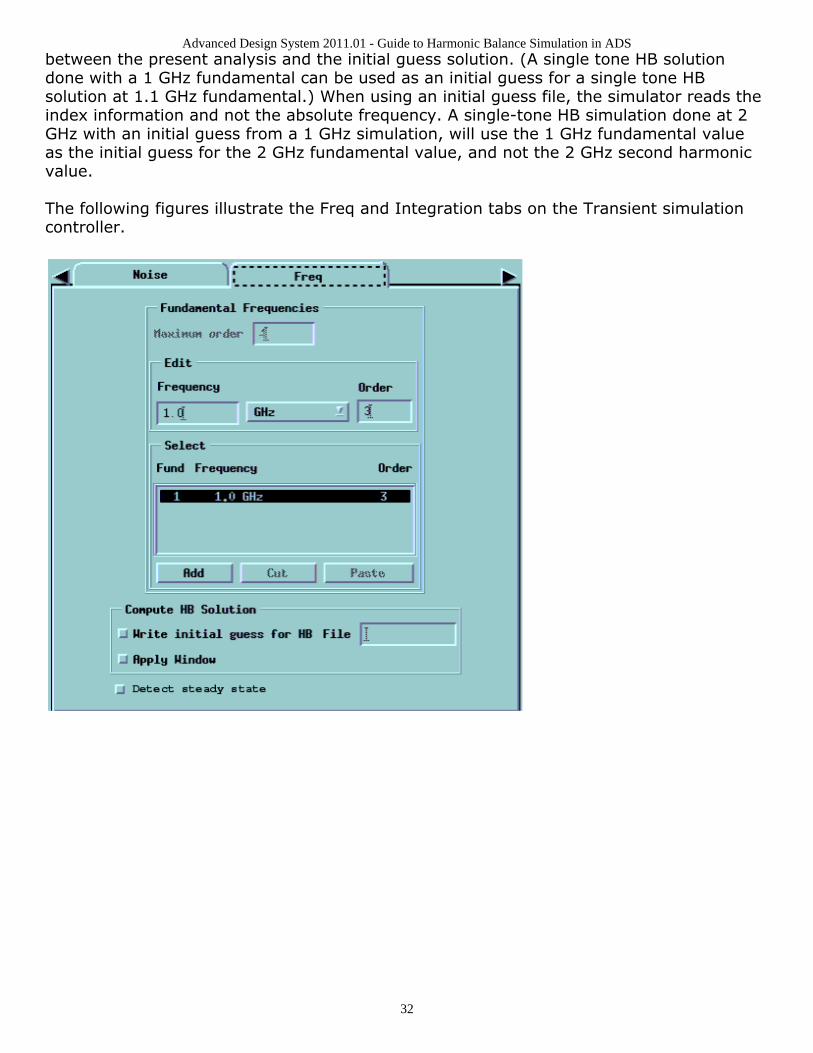
In this example, the frequency of the oscillator is 738 MHz and the divide ratio on thedivider is 2. The transient simulation was run for 90 nsec to determine when the circuitwas near steady state. Then it was re-simulated from 60 to 70 nsec since the circuit wasvery near steady state in that time range. In some cases it may take the circuit longer toreach steady state. It is strongly recommended to plot and verify the transient resultsbefore starting the HB simulation. See the waveform plots of the divider in the followingdiagram.
After generating the initial guess from transient, the single-tone HB simulation wasperformed. The frequency and order were the same as specified in the transient setup,namely Freq[1]=738 MHz and Order=31. Since the circuit had square wave forms, thetransient solution was a very good initial guess for harmonic balance.
TAHB for 2-Tone HB Simulation of a Large Transceiver Circuit
Consider a 2-Tone HB Simulation of a large transceiver circuit that fails to converge due toa very large initial residual. The reason for this is that the DC initial guess is too far awayfrom the actual solution. The circuit uses two tones: LO=2140 MHz and IF=260 MHz. Thecommensurate frequency (greatest common divisor) is 20 MHz. That is a 50 nsec period(13 cycles of the LO and 107 cycles of the IF). The number of periods required for thetransient simulation will depend on how quickly the circuit approaches steady state. Thebest way to determine how fast the circuit approaches steady state is to plot the transientsimulation waveforms. Since the transceiver in this example approaches steady staterelatively quickly, 5 periods of the commensurate period is sufficient: thus the transientStop time should be set to 5*50 nsec = 250 nsec. If the commensurate frequency is smalland that circuit does not approach steady state quickly, the transient simulation tocompute the TAHB initial guess would take a long time. In those cases, it is recommended
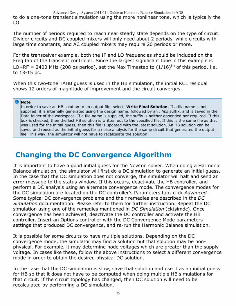
Advanced Design System 2011.01 - Guide to Harmonic Balance Simulation in ADS
35
to do a one-tone transient simulation using the more nonlinear tone, which is typically theLO.
The number of periods required to reach near steady state depends on the type of circuit.Divider circuits and DC coupled mixers will only need about 2 periods, while circuits withlarge time constants, and AC coupled mixers may require 20 periods or more.
For the transceiver example, both the IF and LO frequencies should be included on theFreq tab of the transient controller. Since the largest significant tone in this example isLO+RF = 2400 MHz (208 ps period), set the Max Timestep to (1/16)th of this period, i.e.to 13-15 ps.
When this two-tone TAHB guess is used in the HB simulation, the initial KCL residualshows 12 orders of magnitude of improvement and the circuit converges.
NoteIn order to save an HB solution to an output file, select Write Final Solution. If a file name is notsupplied, it is internally generated using the design name, followed by an . hbs suffix, and is saved in theData folder of the workspace. If a file name is supplied, the suffix is neither appended nor required. If thisbox is checked, then the last HB solution is written out to the specified file. If this is the same file as thatwas used for the initial guess, then this file is updated with the latest solution. An HB solution can besaved and reused as the initial guess for a noise analysis for the same circuit that generated the outputfile. This way, the simulator will not have to recalculate the solution.
Changing the DC Convergence AlgorithmIt is important to have a good initial guess for the Newton solver. When doing a HarmonicBalance simulation, the simulator will first do a DC simulation to generate an initial guess.In the case that the DC simulation does not converge, the simulator will halt and send anerror message to the status window. If this occurs, deactivate the HB controller, andperform a DC analysis using an alternate convergence mode. The convergence modes forthe DC simulation are located on the DC controller's Parameters tab; click Advanced .Some typical DC convergence problems and their remedies are described in the DCSimulation documentation. Please refer to them for further instruction. Repeat the DCsimulation using one of the remedies mentioned in DC Simulation (cktsimdc). Onceconvergence has been achieved, deactivate the DC controller and activate the HBcontroller. Insert an Options controller with the DC Convergence Mode parameterssettings that produced DC convergence, and re-run the Harmonic Balance simulation.
It is possible for some circuits to have multiple solutions. Depending on the DCconvergence mode, the simulator may find a solution but that solution may be non-physical. For example, it may determine node voltages which are greater than the supplyvoltage. In cases like these, follow the above instructions to select a different convergencemode in order to obtain the desired physical DC solution.
In the case that the DC simulation is slow, save that solution and use it as an initial guessfor HB so that it does not have to be computed when doing multiple HB simulations forthat circuit. If the circuit topology has changed, then DC solution will need to berecalculated by performing a DC simulation.
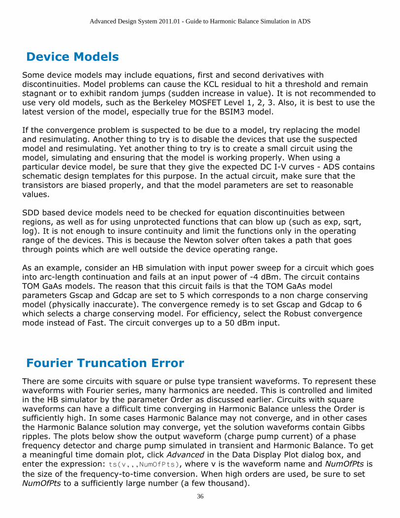
Advanced Design System 2011.01 - Guide to Harmonic Balance Simulation in ADS
36
Device ModelsSome device models may include equations, first and second derivatives withdiscontinuities. Model problems can cause the KCL residual to hit a threshold and remainstagnant or to exhibit random jumps (sudden increase in value). It is not recommended touse very old models, such as the Berkeley MOSFET Level 1, 2, 3. Also, it is best to use thelatest version of the model, especially true for the BSIM3 model.
If the convergence problem is suspected to be due to a model, try replacing the modeland resimulating. Another thing to try is to disable the devices that use the suspectedmodel and resimulating. Yet another thing to try is to create a small circuit using themodel, simulating and ensuring that the model is working properly. When using aparticular device model, be sure that they give the expected DC I-V curves - ADS containsschematic design templates for this purpose. In the actual circuit, make sure that thetransistors are biased properly, and that the model parameters are set to reasonablevalues.
SDD based device models need to be checked for equation discontinuities betweenregions, as well as for using unprotected functions that can blow up (such as exp, sqrt,log). It is not enough to insure continuity and limit the functions only in the operatingrange of the devices. This is because the Newton solver often takes a path that goesthrough points which are well outside the device operating range.
As an example, consider an HB simulation with input power sweep for a circuit which goesinto arc-length continuation and fails at an input power of -4 dBm. The circuit containsTOM GaAs models. The reason that this circuit fails is that the TOM GaAs modelparameters Gscap and Gdcap are set to 5 which corresponds to a non charge conservingmodel (physically inaccurate). The convergence remedy is to set Gscap and Gdcap to 6which selects a charge conserving model. For efficiency, select the Robust convergencemode instead of Fast. The circuit converges up to a 50 dBm input.
Fourier Truncation ErrorThere are some circuits with square or pulse type transient waveforms. To represent thesewaveforms with Fourier series, many harmonics are needed. This is controlled and limitedin the HB simulator by the parameter Order as discussed earlier. Circuits with squarewaveforms can have a difficult time converging in Harmonic Balance unless the Order issufficiently high. In some cases Harmonic Balance may not converge, and in other casesthe Harmonic Balance solution may converge, yet the solution waveforms contain Gibbsripples. The plots below show the output waveform (charge pump current) of a phasefrequency detector and charge pump simulated in transient and Harmonic Balance. To geta meaningful time domain plot, click Advanced in the Data Display Plot dialog box, andenter the expression: ts(v,,,NumOfPts), where v is the waveform name and NumOfPts isthe size of the frequency-to-time conversion. When high orders are used, be sure to setNumOfPts to a sufficiently large number (a few thousand).
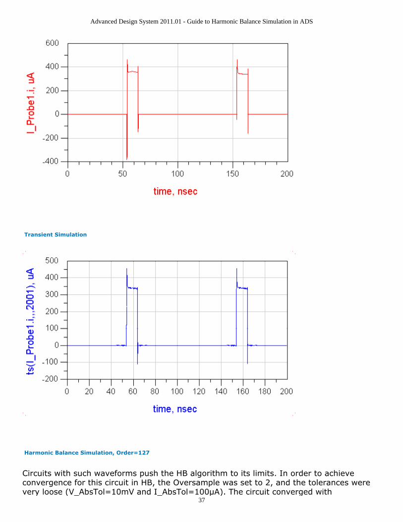
Advanced Design System 2011.01 - Guide to Harmonic Balance Simulation in ADS
37
Transient Simulation
Harmonic Balance Simulation, Order=127
Circuits with such waveforms push the HB algorithm to its limits. In order to achieveconvergence for this circuit in HB, the Oversample was set to 2, and the tolerances werevery loose (V_AbsTol=10mV and I_AbsTol=100µA). The circuit converged with
Advanced Design System 2011.01 - Guide to Harmonic Balance Simulation in ADS
38
Order=127; but even when simulating with Order=511, the accuracy of the solution is notquite acceptable, as seen in the charge pump current plot below. The transient waveform,tran_pump, exhibits a real overshoot. While the HB waveform, hb_pump, tries to matchthis overshoot, due to the limited Order and large HB truncation error it exhibitssignificant Gibbs ripples:
Harmonic Balance Assisted Harmonic BalanceWhen performing a multi-tone harmonic balance simulation, the simulator will decideautomatically which tones to use in generating the final HB solution. This is method isknown as harmonic balance assisted harmonic balance (HBAHB). For example, instead ofsimulating a 3-tone circuit directly, it is possible to simulate a 1-tone, then use the resultas an initial guess for a 2-tone, and finally use that result as an initial guess for the final3-tone simulation. HBAHB is both fast and robust in particular for large multi-tonesimulations of mixer circuits to determine gain and IP3.
HBAHB applies only to multi-tone simulations. By default, this feature is turned on withinthe simulator. The simulator will determine the optimal sequence of tones to simulate.Depending upon various conditions, the simulator may decide to first simulate using a 1-tone then use that result for a 3-tone, and skip the 2-tone simulation.
HBAHB can be found on the Initial Guess tab, in the section called Harmonic BalanceAssisted Harmonic Balance. There are three choices - Off, On, and Auto. The defaultselection is Auto which means that the simulator automatically decides whether or not toperform HBAHB, and the optimal sequence of tones to simulate. The On selection meansthat HBAHB will always simulate each tone up to the last fundamental frequency. In otherwords, a simulation will be performed for each tone. The Off selection means that HBAHBwill not be performed at all. When HBAHB is off, a standard multi-tone HB simulation willtake place.
When using HBAHB, select the Auto convergence mode and the Auto solver type. Both ofthese parameters are found on the Solver tab of the HB controller. This ensures thatsimulating the intermediate tones will be both fast and robust, and not require user-
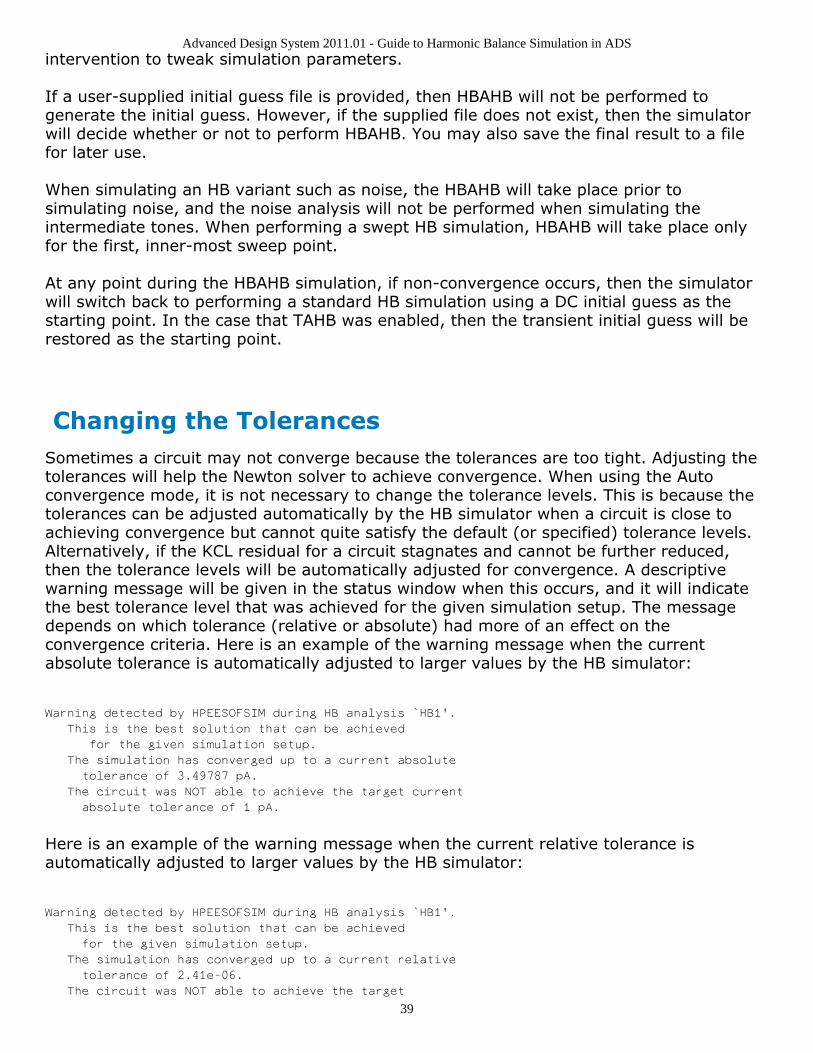
Advanced Design System 2011.01 - Guide to Harmonic Balance Simulation in ADS
39
intervention to tweak simulation parameters.
If a user-supplied initial guess file is provided, then HBAHB will not be performed togenerate the initial guess. However, if the supplied file does not exist, then the simulatorwill decide whether or not to perform HBAHB. You may also save the final result to a filefor later use.
When simulating an HB variant such as noise, the HBAHB will take place prior tosimulating noise, and the noise analysis will not be performed when simulating theintermediate tones. When performing a swept HB simulation, HBAHB will take place onlyfor the first, inner-most sweep point.
At any point during the HBAHB simulation, if non-convergence occurs, then the simulatorwill switch back to performing a standard HB simulation using a DC initial guess as thestarting point. In the case that TAHB was enabled, then the transient initial guess will berestored as the starting point.
Changing the TolerancesSometimes a circuit may not converge because the tolerances are too tight. Adjusting thetolerances will help the Newton solver to achieve convergence. When using the Autoconvergence mode, it is not necessary to change the tolerance levels. This is because thetolerances can be adjusted automatically by the HB simulator when a circuit is close toachieving convergence but cannot quite satisfy the default (or specified) tolerance levels.Alternatively, if the KCL residual for a circuit stagnates and cannot be further reduced,then the tolerance levels will be automatically adjusted for convergence. A descriptivewarning message will be given in the status window when this occurs, and it will indicatethe best tolerance level that was achieved for the given simulation setup. The messagedepends on which tolerance (relative or absolute) had more of an effect on theconvergence criteria. Here is an example of the warning message when the currentabsolute tolerance is automatically adjusted to larger values by the HB simulator:
Warning detected by HPEESOFSIM during HB analysis `HB1'.
This is the best solution that can be achieved
for the given simulation setup.
The simulation has converged up to a current absolute
tolerance of 3.49787 pA.
The circuit was NOT able to achieve the target current
absolute tolerance of 1 pA.
Here is an example of the warning message when the current relative tolerance isautomatically adjusted to larger values by the HB simulator:
Warning detected by HPEESOFSIM during HB analysis `HB1'.
This is the best solution that can be achieved
for the given simulation setup.
The simulation has converged up to a current relative
tolerance of 2.41e-06.
The circuit was NOT able to achieve the target
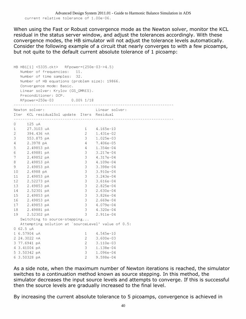
Advanced Design System 2011.01 - Guide to Harmonic Balance Simulation in ADS
40
current relative tolerance of 1.00e-06.
When using the Fast or Robust convergence mode as the Newton solver, monitor the KCLresidual in the status server window, and adjust the tolerances accordingly. With theseconvergence modes, the HB simulator will not adjust the tolerance levels automatically.Consider the following example of a circuit that nearly converges to with a few picoamps,but not quite to the default current absolute tolerance of 1 picoamp:
HB HB1[1] <5335.ckt> RFpower=(250e-03->4.5)
Number of frequencies: 11.
Number of time samples: 32.
Number of HB equations (problem size): 19866.
Convergence mode: Basic.
Linear solver: Krylov (GS_GMRES).
Preconditioner: DCP.
RFpower=250e-03 0.00% 1/18
------------------------------------------------------------------------
Newton solver: Linear solver:
Iter KCL residualSol update Iters Residual
------------------------------------------------------------------------
0 125 uA
1 27.3103 uA 1 4.165e-10
2 394.436 nA 2 1.431e-02
3 553.875 pA 3 1.025e-03
4 2.3978 pA 4 7.406e-05
5 2.49853 pA 4 1.354e-04
6 2.49881 pA 3 3.217e-04
7 2.49852 pA 3 4.317e-04
8 2.49853 pA 3 4.109e-04
9 2.49853 pA 3 3.398e-04
10 2.4988 pA 3 3.910e-04
11 2.49853 pA 3 3.243e-04
12 2.52273 pA 3 3.616e-04
13 2.49853 pA 3 2.825e-04
14 2.52301 pA 3 2.630e-04
15 2.49853 pA 3 3.826e-04
16 2.49853 pA 3 2.669e-04
17 2.49853 pA 3 4.079e-04
18 2.49881 pA 3 4.320e-04
19 2.52302 pA 3 2.911e-04
Switching to source-stepping...
Attempting solution at `sourceLevel' value of 0.5:
0 62.5 uA
1 6.57904 uA 1 4.545e-10
2 24.3022 nA 2 3.600e-03
3 77.6941 pA 2 3.110e-03
4 3.41004 pA 3 1.138e-04
5 3.50342 pA 3 1.096e-04
6 3.50328 pA 2 9.598e-04
As a side note, when the maximum number of Newton iterations is reached, the simulatorswitches to a continuation method known as source stepping. In this method, thesimulator decreases the input source levels and attempts to converge. If this is successfulthen the source levels are gradually increased to the final level.
By increasing the current absolute tolerance to 5 picoamps, convergence is achieved in
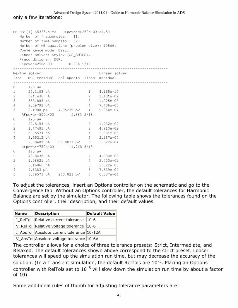
Advanced Design System 2011.01 - Guide to Harmonic Balance Simulation in ADS
41
only a few iterations:
HB HB1[1] <5335.ckt> RFpower=(250e-03->4.5)
Number of frequencies: 11.
Number of time samples: 32.
Number of HB equations (problem size): 19866.
Convergence mode: Basic.
Linear solver: Krylov (GS_GMRES).
Preconditioner: DCP.
RFpower=250e-03 0.00% 1/18
------------------------------------------------------------------------
Newton solver: Linear solver:
Iter KCL residual Sol update Iters Residual
------------------------------------------------------------------------
0 125 uA
1 27.3103 uA 1 4.165e-10
2 394.436 nA 2 1.431e-02
3 553.883 pA 3 1.025e-03
4 2.39792 pA 4 7.406e-05
5 2.4988 pA 4.05239 pV 4 1.354e-04
RFpower=500e-03 5.88% 2/18
0 125 uA
1 29.5154 uA 2 1.232e-02
2 1.47481 uA 2 4.910e-02
3 3.05574 nA 4 2.831e-03
4 3.95315 pA 5 2.187e-04
5 2.00489 pA 85.8831 pV 5 3.522e-04
RFpower=750e-03 11.76% 3/18
0 125 uA
1 43.8438 uA 2 4.030e-02
2 1.08621 uA 4 2.400e-02
3 3.16865 nA 5 2.622e-03
4 4.6383 pA 6 7.839e-04
5 3.69573 pA 260.821 pV 6 6.887e-04
To adjust the tolerances, insert an Options controller on the schematic and go to theConvergence tab. Without an Options controller, the default tolerances for HarmonicBalance are set by the simulator. The following table shows the tolerances found on theOptions controller, their description, and their default values.
Name Description Default Value
I_RelTol Relative current tolerance 10-6
V_RelTol Relative voltage tolerance 10-6
I_AbsTol Absolute current tolerance 10-12A
V_AbsTol Absolute voltage tolerance 10-6V
The controller allows for a choice of three tolerance presets: Strict, Intermediate, andRelaxed. The default tolerances shown above correspond to the strict preset. Loosertolerances will speed up the simulation run time, but may decrease the accuracy of thesolution. (In a Transient simulation, the default RelTols are 10-3. Placing an Optionscontroller with RelTols set to 10-6 will slow down the simulation run time by about a factorof 10).
Some additional rules of thumb for adjusting tolerance parameters are:

Advanced Design System 2011.01 - Guide to Harmonic Balance Simulation in ADS
42
If the currents in the circuit are on the order of miliamps or amps, try increasing therelative current tolerance.If the currents in the circuit are on the order if microamps or smaller, try increasingthe absolute current tolerance.If the status window output shows consecutive values in the Solution update (Solupdate) column, then try increasing the voltage tolerances.
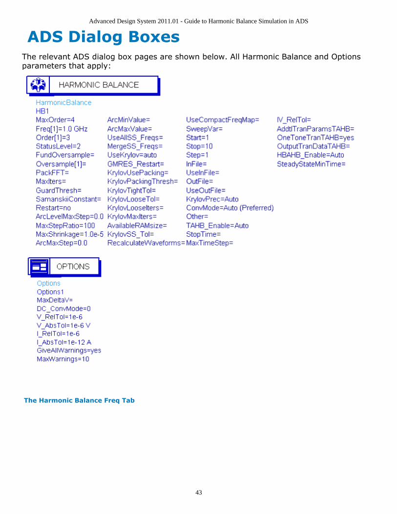
Advanced Design System 2011.01 - Guide to Harmonic Balance Simulation in ADS
43
ADS Dialog BoxesThe relevant ADS dialog box pages are shown below. All Harmonic Balance and Optionsparameters that apply:
The Harmonic Balance Freq Tab
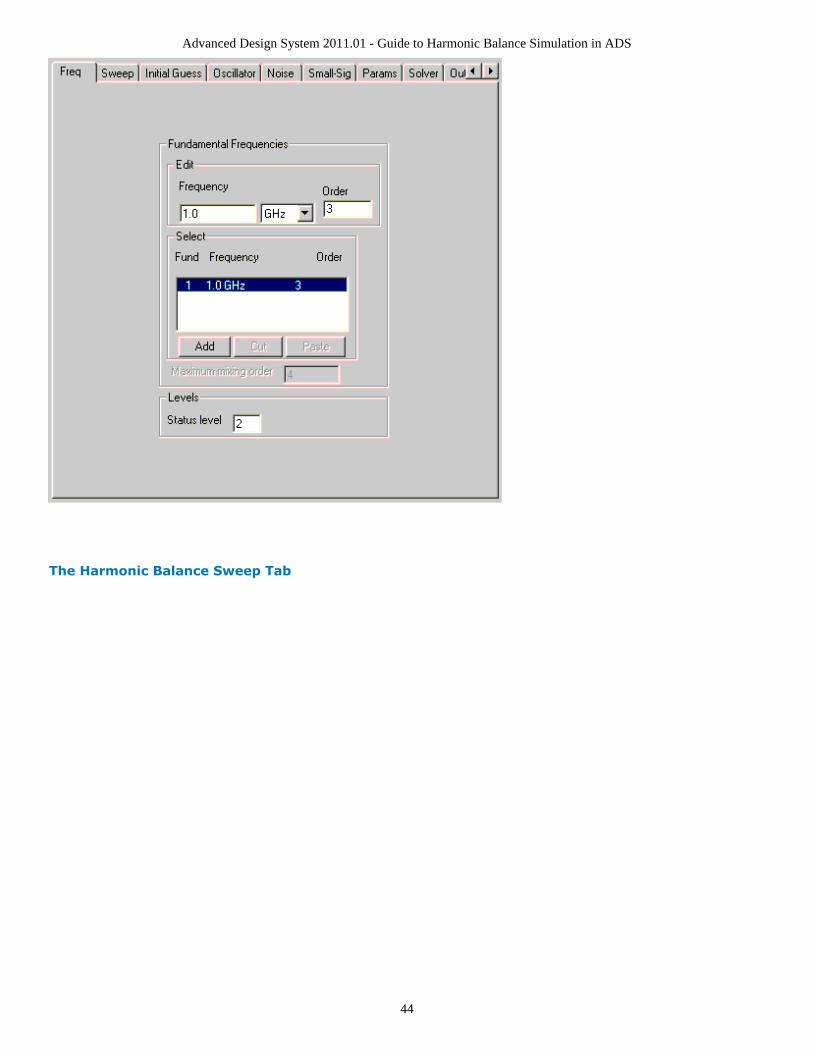
Advanced Design System 2011.01 - Guide to Harmonic Balance Simulation in ADS
44
The Harmonic Balance Sweep Tab
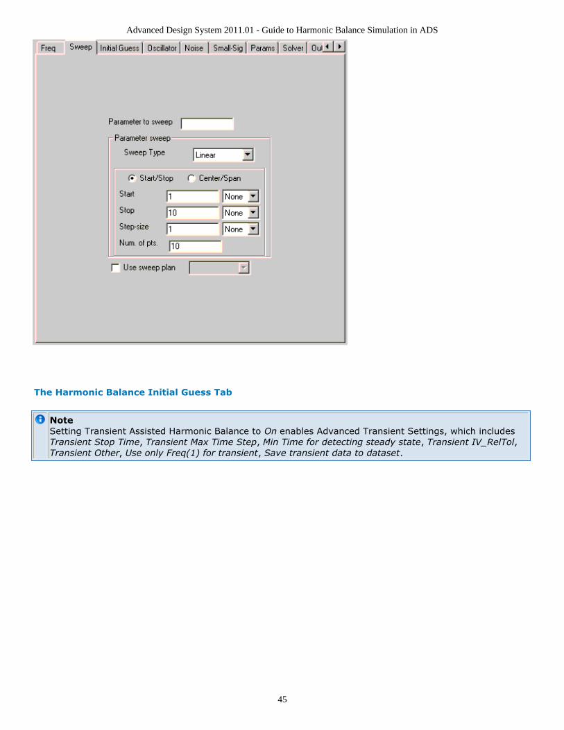
Advanced Design System 2011.01 - Guide to Harmonic Balance Simulation in ADS
45
The Harmonic Balance Initial Guess Tab
NoteSetting Transient Assisted Harmonic Balance to On enables Advanced Transient Settings, which includesTransient Stop Time, Transient Max Time Step, Min Time for detecting steady state, Transient IV_RelTol,Transient Other, Use only Freq(1) for transient, Save transient data to dataset.
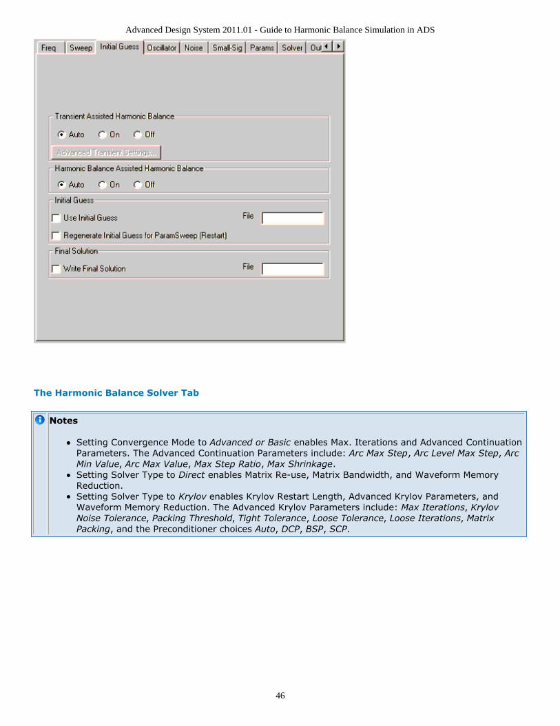
Advanced Design System 2011.01 - Guide to Harmonic Balance Simulation in ADS
46
The Harmonic Balance Solver Tab
Notes
Setting Convergence Mode to Advanced or Basic enables Max. Iterations and Advanced ContinuationParameters. The Advanced Continuation Parameters include: Arc Max Step, Arc Level Max Step, ArcMin Value, Arc Max Value, Max Step Ratio, Max Shrinkage.Setting Solver Type to Direct enables Matrix Re-use, Matrix Bandwidth, and Waveform MemoryReduction.Setting Solver Type to Krylov enables Krylov Restart Length, Advanced Krylov Parameters, andWaveform Memory Reduction. The Advanced Krylov Parameters include: Max Iterations, KrylovNoise Tolerance, Packing Threshold, Tight Tolerance, Loose Tolerance, Loose Iterations, MatrixPacking, and the Preconditioner choices Auto, DCP, BSP, SCP.

Advanced Design System 2011.01 - Guide to Harmonic Balance Simulation in ADS
47
The Harmonic Balance Params Tab
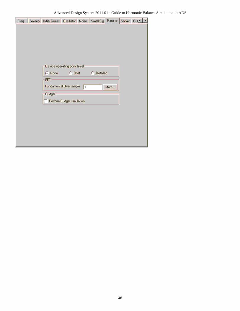
Advanced Design System 2011.01 - Guide to Harmonic Balance Simulation in ADS
48
Advanced Design System 2011.01 - Guide to Harmonic Balance Simulation in ADS
49
Additional ParametersThis section describes some additional parameters which may help nonconverging circuits.These parameters are for the outer (Newton) solver, the inner (Krylov) solver, arc-lengthcontinuation, and for memory issues.
Convergence ModeThe Newton solver has additional settings (hidden parameters) that can be used toenhance its performance and assist convergence
The hidden parameter UseOptDamp turns on the optimal damping search. Thedefault is set to off, or 0. To turn this parameter on, set it to on, or 1. This parametermay be used with auto or advanced convergence modes.The parameter RedRatio is the KCL residual reduction threshold, default is 0.99.This is the ratio by which the norm of the solution vector must be reduced from oneiteration to the next. This parameter has to be smaller than 1. Reducing RedRatio canaccelerate the convergence rate at the cost of diminished robustness. This parametermay be used with auto or advanced convergence modes.The parameter NormCheck is the type of norm used in determining whether theKCL residual has converged. The default is set to 1, which corresponds to the L-1norm. Other possible values include 0 (L-infinity norm), and 2 (L-2 norm). The L-infinity norm is the most conservative, followed by the L-2 and L-1 normsrespectively. The L-2 and L-infinity norms are recommended for highly nonlinearlarge circuits. For a definition of these norms, consider the vector x of size n. Then,the L-1 norm is defined as||x||1 := |x1 |...|xn|,
the L-2 norm is defined as||x||2 := (|x1 |2 +...+|xn|2) 1/2,
and the L-infinity norm is defined as||x||inf :=max |xi |, for 1<=i<=n.
This parameter may be used with auto, advanced, or basic convergence modes.
Krylov SolverAdditional Krylov parameters can be found on the HB controller's Solver tab after clickingAdvanced Krylov Parameters. It is strongly recommended to use caution when adjustingthese parameters, as they are very specific to the internal algorithms.
The parameter Maximum number of iterations (KrylovMaxIters on schematic) is themaximum number of Krylov solver iterations allowed. The default is intentionally set to alarge value of 150 to accommodate even slowly convergent iterations. Increase thisnumber in cases where poor convergence may be improved and an increase in simulation
Advanced Design System 2011.01 - Guide to Harmonic Balance Simulation in ADS
50
run time is acceptable.
The parameter Krylov Restart Length (GMRES_Restart on schematic) sets the numberof iterations after which the Krylov linear solver restarts. At this point the algorithm doesnot need data from previous steps, and the corresponding memory is released. Thus,smaller values lead to lower memory requirements, but might significantly affectconvergence. The default is set to Robust, and it is strongly recommended that you avoiddecreasing this value unless the problem is extremely large and convergence is carefullymonitored. Larger values offer potentially more robust performance, but require morememory. If there are memory constraints, then set this value to 50 or lower by enteringthe value in the Custom dialog box entry.
The solver achieves full convergence if the Krylov solver residual is less than the tighttolerance, which is set by the parameter Tight Tolerance (default value of 0.001). Afterthe number of iterations specified by the parameter Loose Iterations (default value of50), the solver then uses parameter Loose Tolerance to achieve partial convergence.The loose tolerance has default value of 0.1. The Krylov solver fails to converge if theresidual reduction factor from two adjacent iterations becomes larger than the parameterKrylovConvRatio, which has default set to 0.9. The KrylovConvRatio is a hiddenparameter, whereas the other three mentioned above are in the HB controller's Solver tabby clicking Advanced Krylov Parameters.
A hidden parameter for the DCP preconditioner:
PrecMatrixSolver sets the matrix solver for the DCP preconditioner. Two solvers areavailable currently: the general solver that is preferable for smaller or typical-sizecircuits, and the large-circuit solver that is preferable for larger circuits. Allowedvalues are:
PrecMatrixSolver=0 (default, the simulator automatically chooses the solver)PrecMatrixSolver=1 (use the general solver)PrecMatrixSolver=2 (use the large-circuit solver)
Some hidden parameters for the BSP and SCP preconditioners:
PrecRhsThresh activate BSP or SCP if Newton residual is smaller than thisthreshold (default=0.05) _ScpSchurSolver selects the Schur solver in SCP, 0=DMRES (default), 1=GMRES _ScpReuse 1=re-use the SCP at each Newton iteration (default), 0=reload the SCPat each Newton iteration _ScpTol inner SCP Schur solver tolerance (default=0.001) _ScpStartIter use SCP from this Newton iteration onward (default=0)
Arc Length ContinuationThe simulator will switch over to arc-length continuation method when it is having adifficult time converging using the Direct solver. This algorithm is very robust. If thesimulator goes into this method, it is often the case that the circuit has instabilities ormultiple solutions. It is recommended to try all other convergence remedies first before
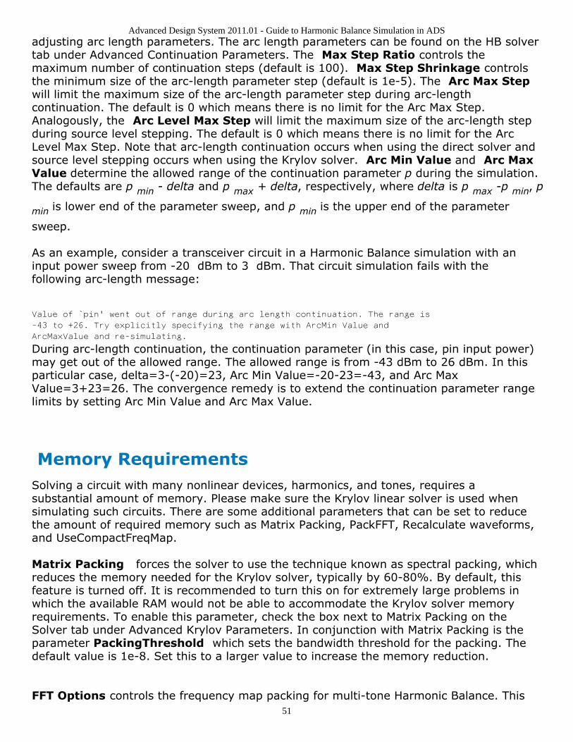
Advanced Design System 2011.01 - Guide to Harmonic Balance Simulation in ADS
51
adjusting arc length parameters. The arc length parameters can be found on the HB solvertab under Advanced Continuation Parameters. The Max Step Ratio controls themaximum number of continuation steps (default is 100). Max Step Shrinkage controlsthe minimum size of the arc-length parameter step (default is 1e-5). The Arc Max Stepwill limit the maximum size of the arc-length parameter step during arc-lengthcontinuation. The default is 0 which means there is no limit for the Arc Max Step.Analogously, the Arc Level Max Step will limit the maximum size of the arc-length stepduring source level stepping. The default is 0 which means there is no limit for the ArcLevel Max Step. Note that arc-length continuation occurs when using the direct solver andsource level stepping occurs when using the Krylov solver. Arc Min Value and Arc MaxValue determine the allowed range of the continuation parameter p during the simulation.The defaults are p min - delta and p max + delta, respectively, where delta is p max -p min, p
min is lower end of the parameter sweep, and p min is the upper end of the parameter
sweep.
As an example, consider a transceiver circuit in a Harmonic Balance simulation with aninput power sweep from -20 dBm to 3 dBm. That circuit simulation fails with thefollowing arc-length message:
Value of `pin' went out of range during arc length continuation. The range is
-43 to +26. Try explicitly specifying the range with ArcMin Value and
ArcMaxValue and re-simulating.
During arc-length continuation, the continuation parameter (in this case, pin input power)may get out of the allowed range. The allowed range is from -43 dBm to 26 dBm. In thisparticular case, delta=3-(-20)=23, Arc Min Value=-20-23=-43, and Arc MaxValue=3+23=26. The convergence remedy is to extend the continuation parameter rangelimits by setting Arc Min Value and Arc Max Value.
Memory RequirementsSolving a circuit with many nonlinear devices, harmonics, and tones, requires asubstantial amount of memory. Please make sure the Krylov linear solver is used whensimulating such circuits. There are some additional parameters that can be set to reducethe amount of required memory such as Matrix Packing, PackFFT, Recalculate waveforms,and UseCompactFreqMap.
Matrix Packing forces the solver to use the technique known as spectral packing, whichreduces the memory needed for the Krylov solver, typically by 60-80%. By default, thisfeature is turned off. It is recommended to turn this on for extremely large problems inwhich the available RAM would not be able to accommodate the Krylov solver memoryrequirements. To enable this parameter, check the box next to Matrix Packing on theSolver tab under Advanced Krylov Parameters. In conjunction with Matrix Packing is theparameter PackingThreshold which sets the bandwidth threshold for the packing. Thedefault value is 1e-8. Set this to a larger value to increase the memory reduction.
FFT Options controls the frequency map packing for multi-tone Harmonic Balance. This
Advanced Design System 2011.01 - Guide to Harmonic Balance Simulation in ADS
52
parameter can be selected to either minimize aliasing or minimize memory usage andsimulation run time. By default the simulator sets the parameter to minimize memoryusage and simulation run time. Minimizing the memory usage may improve the simulationspeed and reduce memory consumption by using a smaller number of time samples(smaller FFTs), but at the potential loss of dynamic range and accuracy due to the aliasedharmonics of the first fundamental now possibly landing on various mixing tones. Formixers and other applications with a single large dominant (LO) tone, that frequencyshould be assigned to the first fundamental and FFT Options should be set to minimizealiasing so that any aliased harmonics of this large signal will just land on its ownharmonics and not on mixing terms. If you are simulating mixer intermodulation or third-order intercept, it is recommended that this parameter also be set to minimize aliasing toachieve the most accurate results.
Both use dynamic waveform recalculation and use compact frequency map formemory reduction. When using neither of these, all nodal waveforms are stored. Theadvantage is that it speeds up simulation time since the waveforms do not need to berecalculated. However, the disadvantage is that storing all the nodal waveforms causes ahigh memory consumption.
The parameter Use dynamic waveform recalculation (found on the Solver tab of the HBcontroller) enables reuse of dynamic waveform memory instead of up front storage on allwaveforms. By enabling this parameter, only the needed waveforms are stored whichrequires less memory. However, if two devices are sharing the same node, then thewaveform for the second node would need to be recomputed and therefore result in anincrease in simulation time. Small circuits might simulate a little slower, but notsignificantly.
Use compact frequency map (found on the HB controller's Solver tab) enables a spectralcompression, typically requiring less memory for individual waveforms. If the memoryrequired for the Krylov solver is greater than the available RAM, then this parameter willget set to yes by the simulator and a warning message will be displayed in the statuswindow. By enabling this parameter, simulation speed will increase, yet there is lessmemory reduction compared to using RecalculateWaveforms.
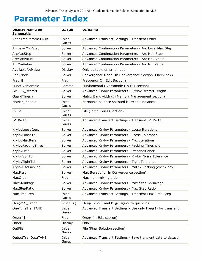
Advanced Design System 2011.01 - Guide to Harmonic Balance Simulation in ADS
53
Parameter IndexDisplay Name onSchematic
UI Tab UI Name
AddtlTranParamsTAHB InitialGuess
Advanced Transient Settings - Transient Other
ArcLevelMaxStep Solver Advanced Continuation Parameters - Arc Level Max Step
ArcMaxStep Solver Advanced Continuation Parameters - Arc Max Step
ArcMaxValue Solver Advanced Continuation Parameters - Arc Max Value
ArcMinValue Solver Advanced Continuation Parameters - Arc Min Value
AvailableRAMsize Display Only editable on schematic
ConvMode Solver Convergence Mode (In Convergence Section, Check box)
Freq[i] Freq Frequency (In Edit Section)
FundOversample Params Fundamental Oversample (In FFT section)
GMRES_Restart Solver Advanced Krylov Parameters - Krylov Restart Length
GuardThresh Solver Matrix Bandwidth (In Memory Management section)
HBAHB_Enable InitialGuess
Harmonic Balance Assisted Harmonic Balance
InFile InitialGuess
File (Initial Guess section)
IV_RelTol InitialGuess
Advanced Transient Settings - Transient IV_RelTol
KrylovLooseIters Solver Advanced Krylov Parameters - Loose Iterations
KrylovLooseTol Solver Advanced Krylov Parameters - Loose Tolerance
KrylovMaxIters Solver Advanced Krylov Parameters - Max Iterations
KrylovPackingThresh Solver Advanced Krylov Parameters - Packing Threshold
KrylovPrec Solver Advanced Krylov Parameters - Preconditioner
KrylovSS_Tol Solver Advanced Krylov Parameters - Krylov Noise Tolerance
KrylovTightTol Solver Advanced Krylov Parameters - Tight Tolerance
KrylovUsePacking Solver Advanced Krylov Parameters - Matrix Packing (check box)
MaxIters Solver Max Iterations (In Convergence section)
MaxOrder Freq Maximum mixing order
MaxShrinkage Solver Advanced Krylov Parameters - Max Step Shrinkage
MaxStepRatio Solver Advanced Krylov Parameters - Max Step Ratio
MaxTimeStep InitialGuess
Advanced Transient Settings - Transient Max Time Step
MergeSS_Freqs Small-Sig Merge small- and large-signal frequencies
OneToneTranTAHB InitialGuess
Advanced Transient Settings - Use only Freq(1) for transient
Order[i] Freq Order (in Edit section)
Other Display Other
OutFile InitialGuess
File (Final Solution section)
OutputTranDataTAHB InitialGuess
Advanced Transient Settings - Save transient data to dataset
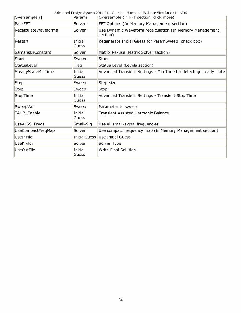
Advanced Design System 2011.01 - Guide to Harmonic Balance Simulation in ADS
54
Oversample[i] Params Oversample (in FFT section, click more)
PackFFT Solver FFT Options (In Memory Management section)
RecalculateWaveforms Solver Use Dynamic Waveform recalculation (In Memory Managementsection)
Restart InitialGuess
Regenerate Initial Guess for ParamSweep (check box)
SamanskiiConstant Solver Matrix Re-use (Matrix Solver section)
Start Sweep Start
StatusLevel Freq Status Level (Levels section)
SteadyStateMinTime InitialGuess
Advanced Transient Settings - Min Time for detecting steady state
Step Sweep Step-size
Stop Sweep Stop
StopTime InitialGuess
Advanced Transient Settings - Transient Stop Time
SweepVar Sweep Parameter to sweep
TAHB_Enable InitialGuess
Transient Assisted Harmonic Balance
UseAllSS_Freqs Small-Sig Use all small-signal frequencies
UseCompactFreqMap Solver Use compact frequency map (in Memory Management section)
UseInFile InitialGuess Use Initial Guess
UseKrylov Solver Solver Type
UseOutFile InitialGuess
Write Final Solution

Advanced Design System 2011.01 - Guide to Harmonic Balance Simulation in ADS
55
Harmonic Balance BackgroundHarmonic Balance is a frequency domain analysis technique for simulating nonlinearcircuits and systems. This method assumes the input stimulus consists of a relatively fewsteady state sinusoids. Therefore the solution can be expressed as a sum of steady statesinusoids that includes the input frequencies in addition to any significant harmonics ormixing terms.
A circuit with a single input source will require a single tone HB simulation. A solutionwaveform (e.g. the node voltage v(t)) in a single tone HB simulation is approximated asfollows:
where f is the fundamental frequency of the source, the Vk's are the complex Fouriercoefficients that the HB analysis computes, and K is the level of truncation (number ofharmonics).
A circuit with multiple input sources will require a multitone HB simulation. In this case,the steady state solution waveforms are approximated with a multidimensional truncatedFourier series as follows:
where n is the number of tones (sources), f 1...n are the fundamental frequencies of each
source, and K1...n are the number of harmonics for each tone. When having multiple tones
in a circuit, mixing products will occur.
The circuit simulator converts N nonlinear differential equations (where N is the size of thecircuit, i.e., the number of nodes and branch currents) into the frequency domain, whereit becomes a set of N*M nonlinear algebraic equations (where M is the total number offrequencies including the input frequencies, their harmonics, and mixing terms), as shownbelow:
where Fk is the k th spectral component of a Fourier transformation, and wk=2*pi*f*k. The
harmonic balance simulator then must simultaneously solve this set of N*M nonlinearalgebraic equations for the Vk values. The number of nonlinear equations that must besolved has increased by a factor of M compared to standard time domain simulators. Thismeans that the matrix sizes and memory requirements of harmonic balance increaseconsiderably as M becomes large. The nonlinear devices are still evaluated in the timedomain by using an inverse Fourier transformation to convert the V values into the v(t)
Advanced Design System 2011.01 - Guide to Harmonic Balance Simulation in ADS
56
k
waveform prior to evaluating the nonlinear q() and g() functions. The current andnonlinear charge waveforms are transformed into the frequency domain at each iterationso their spectral values can be used in the frequency domain equations. Since the HBsimulator uses the Newton's method, the derivatives (nonlinear resistance andcapacitance) must also be computed in the time domain and transformed into thefrequency domain.
The primary advantage of harmonic balance over time domain solutions is that the lineardevices with arbitrary frequency responses can be easily, yet quickly, modeled. Lumpedelement approximations are no longer required. Time domain convolution has beenreplaced with simple frequency domain multiplication. This is especially important for RF,microwave and millimeter frequencies, which are often characterized with measuredfrequency data. An additional benefit is that harmonic balance solutions directly providethe steady state solution without having to wait until the transient solution dies out. Forhigh Q circuits this can be a costly wait. The input stimulus frequencies, f, can also bearbitrarily widely spaced and may actually be non-commensurate, but the harmonicbalance solution can still be quickly obtained. The complexity and cost of the solution doesnot increase just because there is a low frequency tone (a long period) coexisting withhigh frequency tones (very small time steps).
The limitations of harmonic balance are that the signal must be quasi-periodic; they mustbe representable as a sum of a relatively few number M of discrete tones. As M becomeslarge, the amount of required internal memory becomes excessive since the internalmatrix size grows as M2. Using Krylov linear solvers instead of direct methods reduces thememory growth from quadratic to linear (proportional to M). The Krylov solvers thereforeenable harmonic balance to be used on very large circuits and circuits with a large numberof tones.
Harmonic balance is usually the method of choice for simulating analog RF and microwaveproblems, since these are most naturally handled in the frequency domain. Examples ofdevices and circuits suited to this analysis include power amplifiers, frequency multipliers,mixers, and modulators under large signal sinusoidal drive. In the context of highfrequency circuit and system simulation, harmonic balance has a number of advantagesover conventional time-domain analysis:
Designers are usually most interested in a system's steady state behavior. Many highfrequency circuits contain long time constants the require conventional transientmethods to integrate over many periods of the lowest-frequency. Transient analysiswould require integration over an enormous number of periods on the highest-frequency sinusoid.The applied voltage sources are typically multitone sinusoids that may have verynarrow or very widely spaced frequencies. It is not uncommon for the highestfrequency present in the response to be many orders of magnitude greater than thelowest frequency. Transient analysis would require integration over an enormousnumber of periods of the highest frequency sinusoid.The time involved in carrying outthe integration is prohibitive in many practical cases.At high frequencies, many linear models are best represented in the frequencydomain. Simulating such elements in the time domain by means of convolution canresult in problems related to accuracy, causality, or stability.
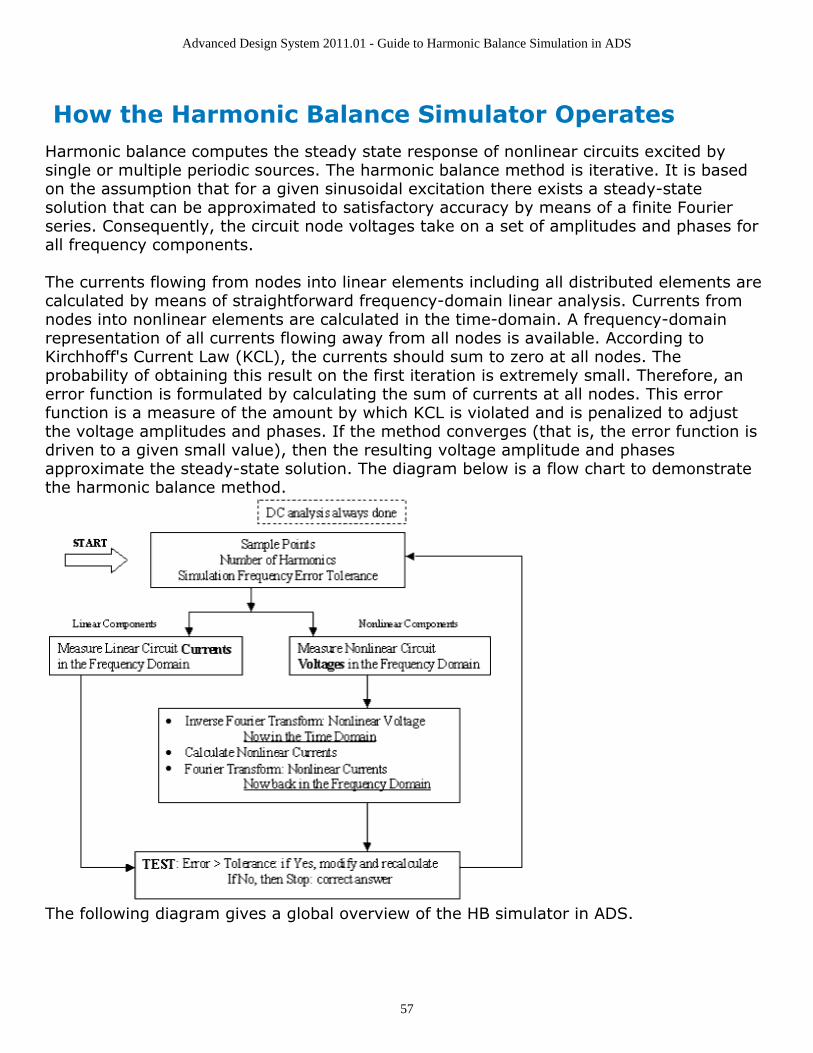
Advanced Design System 2011.01 - Guide to Harmonic Balance Simulation in ADS
57
How the Harmonic Balance Simulator OperatesHarmonic balance computes the steady state response of nonlinear circuits excited bysingle or multiple periodic sources. The harmonic balance method is iterative. It is basedon the assumption that for a given sinusoidal excitation there exists a steady-statesolution that can be approximated to satisfactory accuracy by means of a finite Fourierseries. Consequently, the circuit node voltages take on a set of amplitudes and phases forall frequency components.
The currents flowing from nodes into linear elements including all distributed elements arecalculated by means of straightforward frequency-domain linear analysis. Currents fromnodes into nonlinear elements are calculated in the time-domain. A frequency-domainrepresentation of all currents flowing away from all nodes is available. According toKirchhoff's Current Law (KCL), the currents should sum to zero at all nodes. Theprobability of obtaining this result on the first iteration is extremely small. Therefore, anerror function is formulated by calculating the sum of currents at all nodes. This errorfunction is a measure of the amount by which KCL is violated and is penalized to adjustthe voltage amplitudes and phases. If the method converges (that is, the error function isdriven to a given small value), then the resulting voltage amplitude and phasesapproximate the steady-state solution. The diagram below is a flow chart to demonstratethe harmonic balance method.
The following diagram gives a global overview of the HB simulator in ADS.
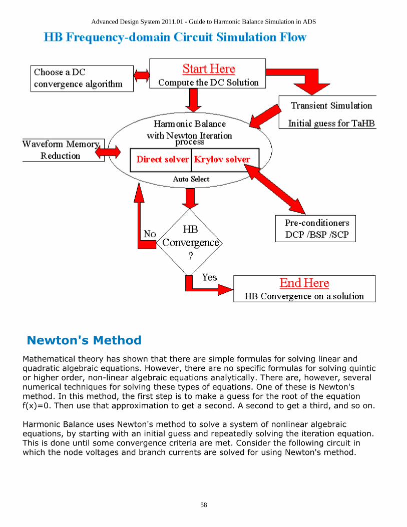
Advanced Design System 2011.01 - Guide to Harmonic Balance Simulation in ADS
58
Newton's MethodMathematical theory has shown that there are simple formulas for solving linear andquadratic algebraic equations. However, there are no specific formulas for solving quinticor higher order, non-linear algebraic equations analytically. There are, however, severalnumerical techniques for solving these types of equations. One of these is Newton'smethod. In this method, the first step is to make a guess for the root of the equationf(x)=0. Then use that approximation to get a second. A second to get a third, and so on.
Harmonic Balance uses Newton's method to solve a system of nonlinear algebraicequations, by starting with an initial guess and repeatedly solving the iteration equation.This is done until some convergence criteria are met. Consider the following circuit inwhich the node voltages and branch currents are solved for using Newton's method.
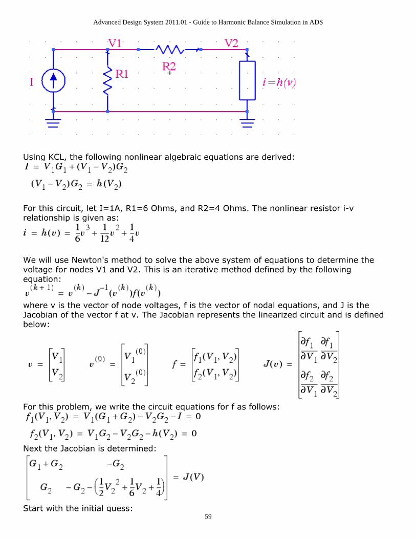
Advanced Design System 2011.01 - Guide to Harmonic Balance Simulation in ADS
59
Using KCL, the following nonlinear algebraic equations are derived:
For this circuit, let I=1A, R1=6 Ohms, and R2=4 Ohms. The nonlinear resistor i-vrelationship is given as:
We will use Newton's method to solve the above system of equations to determine thevoltage for nodes V1 and V2. This is an iterative method defined by the followingequation:
where v is the vector of node voltages, f is the vector of nodal equations, and J is theJacobian of the vector f at v. The Jacobian represents the linearized circuit and is definedbelow:
For this problem, we write the circuit equations for f as follows:
Next the Jacobian is determined:
Start with the initial guess:
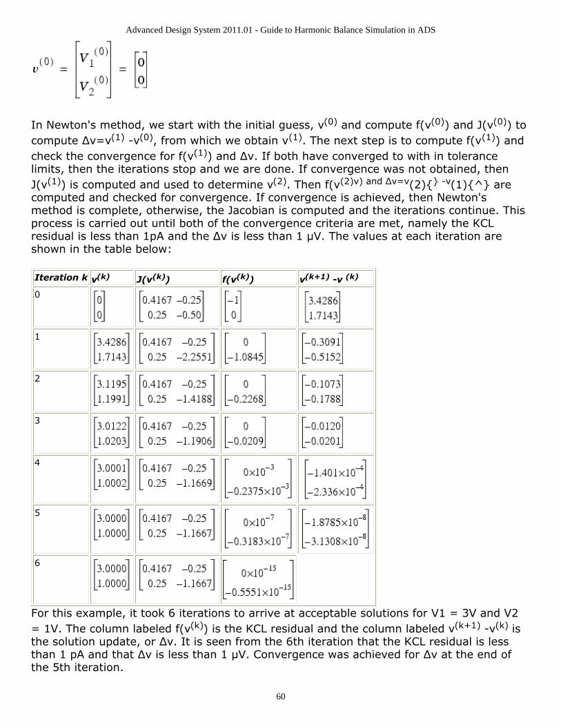
Advanced Design System 2011.01 - Guide to Harmonic Balance Simulation in ADS
60
In Newton's method, we start with the initial guess, v(0) and compute f(v(0)) and J(v(0)) tocompute Δv=v(1) -v(0), from which we obtain v(1). The next step is to compute f(v(1)) andcheck the convergence for f(v(1)) and Δv. If both have converged to with in tolerancelimits, then the iterations stop and we are done. If convergence was not obtained, thenJ(v(1)) is computed and used to determine v(2). Then f(v(2)v) and Δv=v(2){} -v(1){^} arecomputed and checked for convergence. If convergence is achieved, then Newton'smethod is complete, otherwise, the Jacobian is computed and the iterations continue. Thisprocess is carried out until both of the convergence criteria are met, namely the KCLresidual is less than 1pA and the Δv is less than 1 µV. The values at each iteration areshown in the table below:
Iteration k v(k) J(v(k)) f(v(k)) v(k+1) -v (k)
0
1
2
3
4
5
6
For this example, it took 6 iterations to arrive at acceptable solutions for V1 = 3V and V2= 1V. The column labeled f(v(k)) is the KCL residual and the column labeled v(k+1) -v(k) isthe solution update, or Δv. It is seen from the 6th iteration that the KCL residual is lessthan 1 pA and that Δv is less than 1 µV. Convergence was achieved for Δv at the end ofthe 5th iteration.
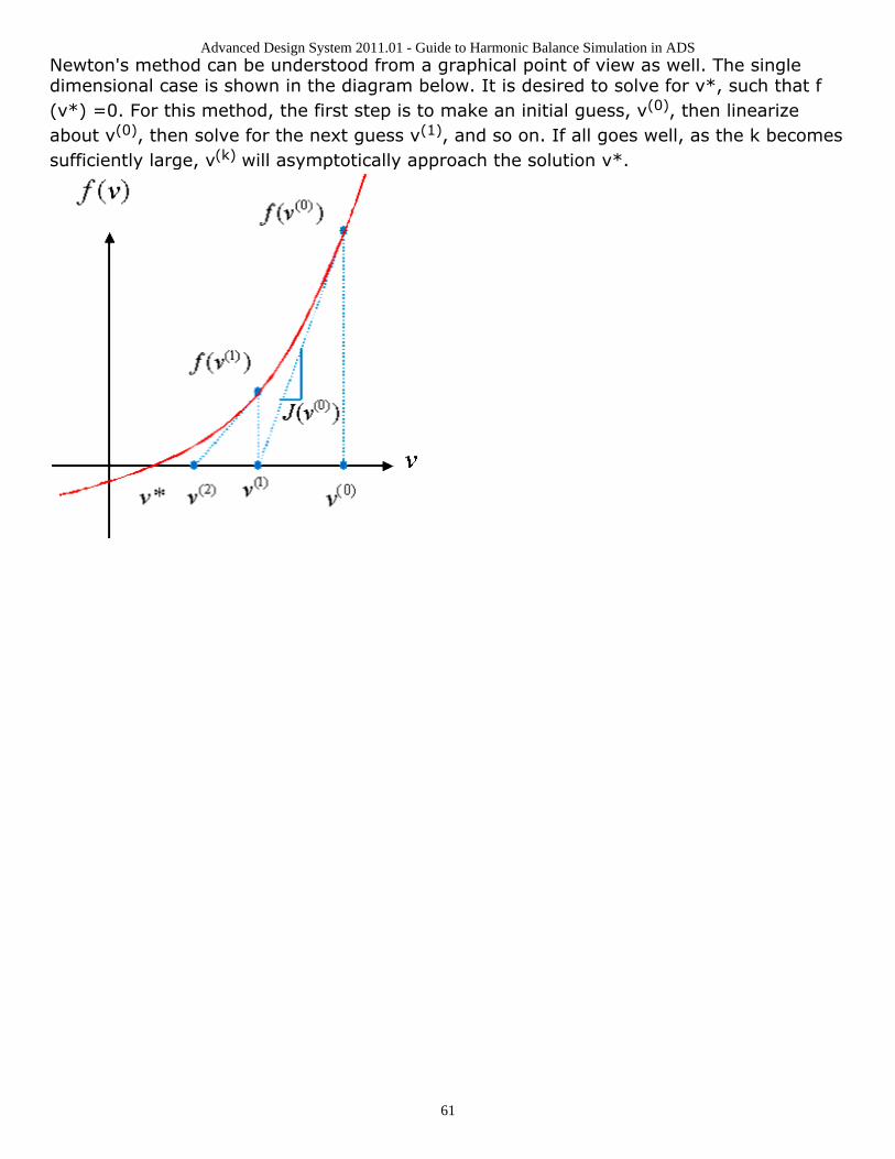
Advanced Design System 2011.01 - Guide to Harmonic Balance Simulation in ADS
61
Newton's method can be understood from a graphical point of view as well. The singledimensional case is shown in the diagram below. It is desired to solve for v*, such that f(v*) =0. For this method, the first step is to make an initial guess, v(0), then linearizeabout v(0), then solve for the next guess v(1), and so on. If all goes well, as the k becomessufficiently large, v(k) will asymptotically approach the solution v*.


![i .] APPROXIMATING HARMONIC FUNCTIONS 499€¦ · APPROXIMATING HARMONIC FUNCTIONS 499 THE APPROXIMATION OF HARMONIC FUNCTIONS BY HARMONIC POLYNOMIALS AND BY HARMONIC RATIONAL FUNCTIONS*](https://static.documents.pub/doc/80x56/5f0873ba7e708231d42214c2/i-approximating-harmonic-functions-499-approximating-harmonic-functions-499-the.jpg)


