AN EVALUATION OF LONG-TERM AIR QUALITY TRENDS IN NORTH TEXAS

USING STATISTICAL AND MACHINE LEARNING TECHNIQUES

Guo Quan Lim

Dissertation Prepared for the Degree of

DOCTOR OF PHILOSOPHY

UNIVERSITY OF NORTH TEXAS

May 2020

APPROVED: Kuruvilla John, Major Professor and

Chair of the Department of Mechanical and Energy Engineering

Hamid Sadat-Hosseini, Committee Member

Sheldon Shi, Committee Member Chetan Tiwari, Committee Member Richard Zhang, Committee Member Hanchen Huang, Dean of the College of

Engineering Victor Prybutok, Dean of the Toulouse

Graduate School

Lim, Guo Quan. An Evaluation of Long-Term Air Quality Trends in North Texas Using

Statistical and Machine Learning Techniques. Doctor of Philosophy (Mechanical and Energy

Engineering), May 2020, 167 pp., 14 tables, 48 figures, 2 appendices, 184 numbered

references.

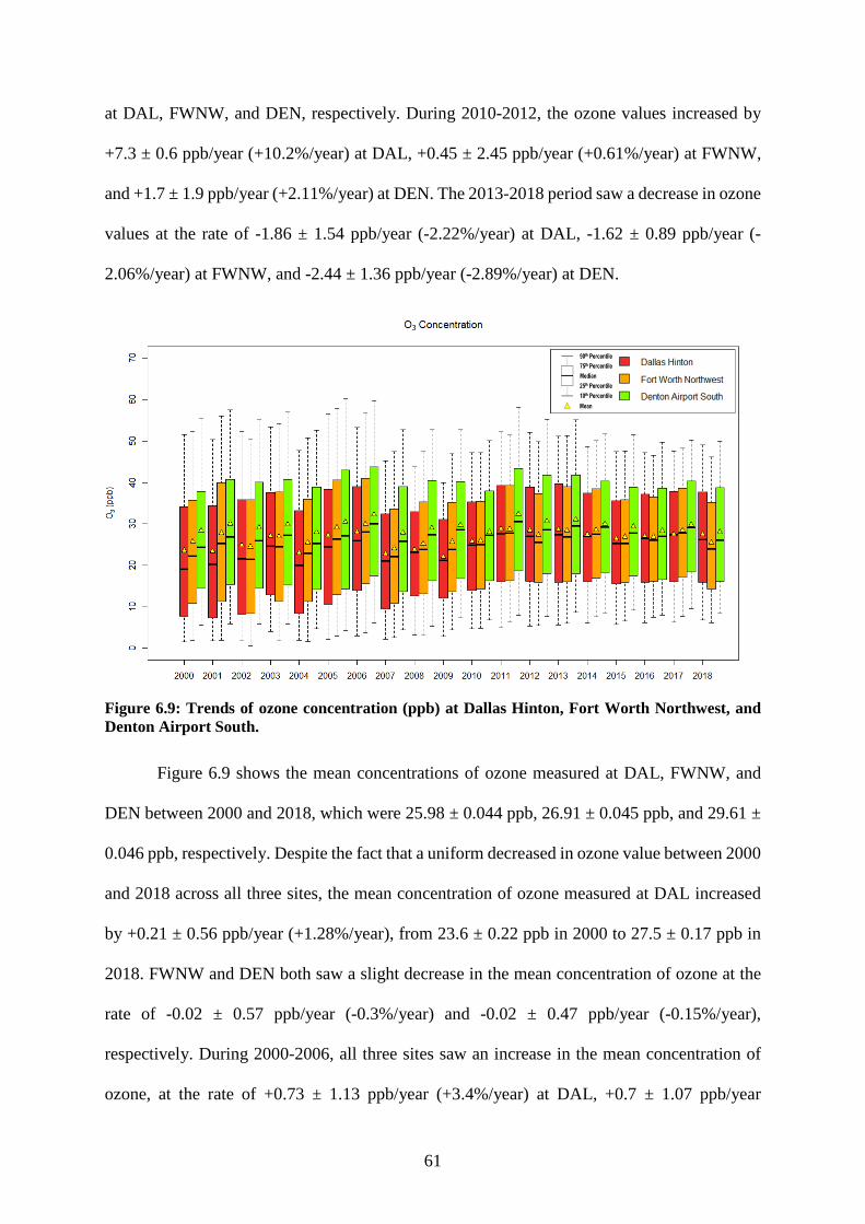
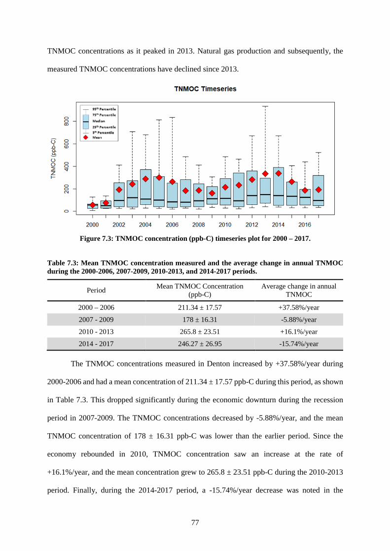
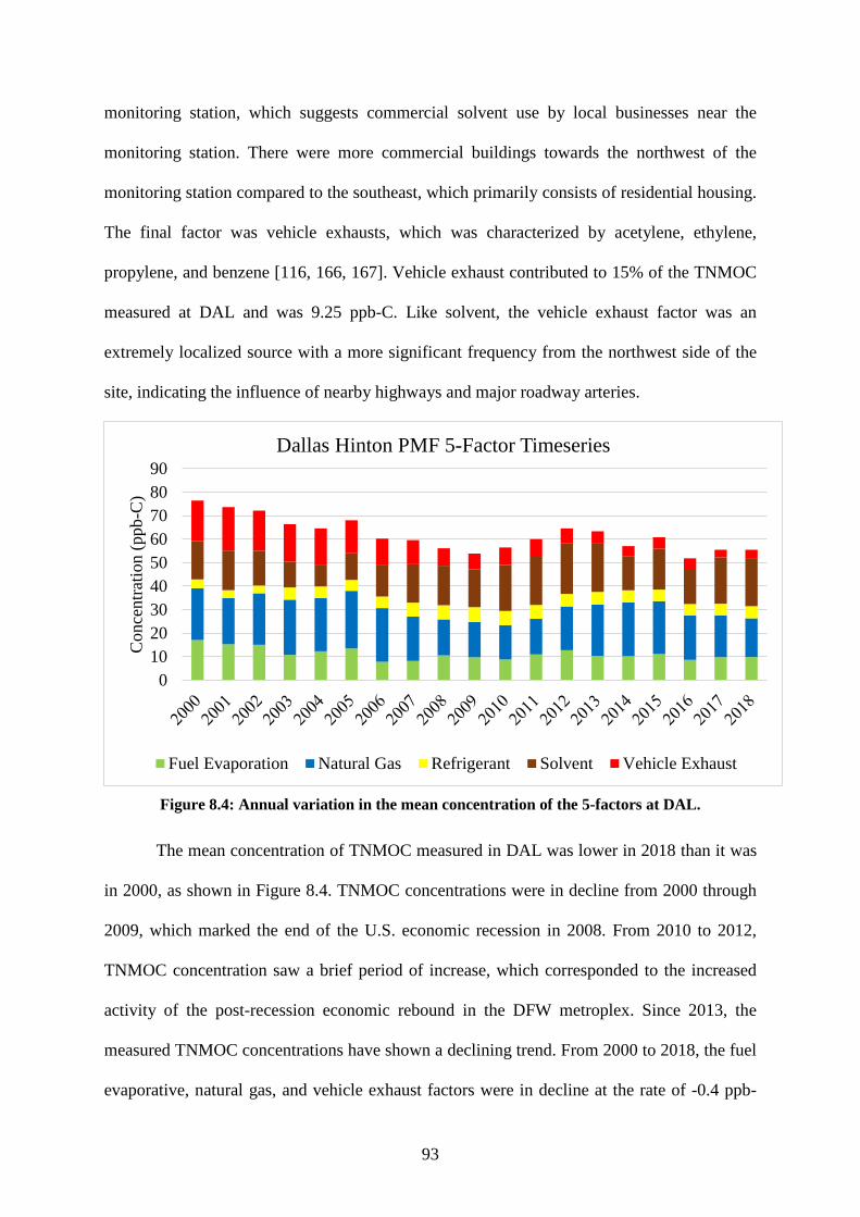
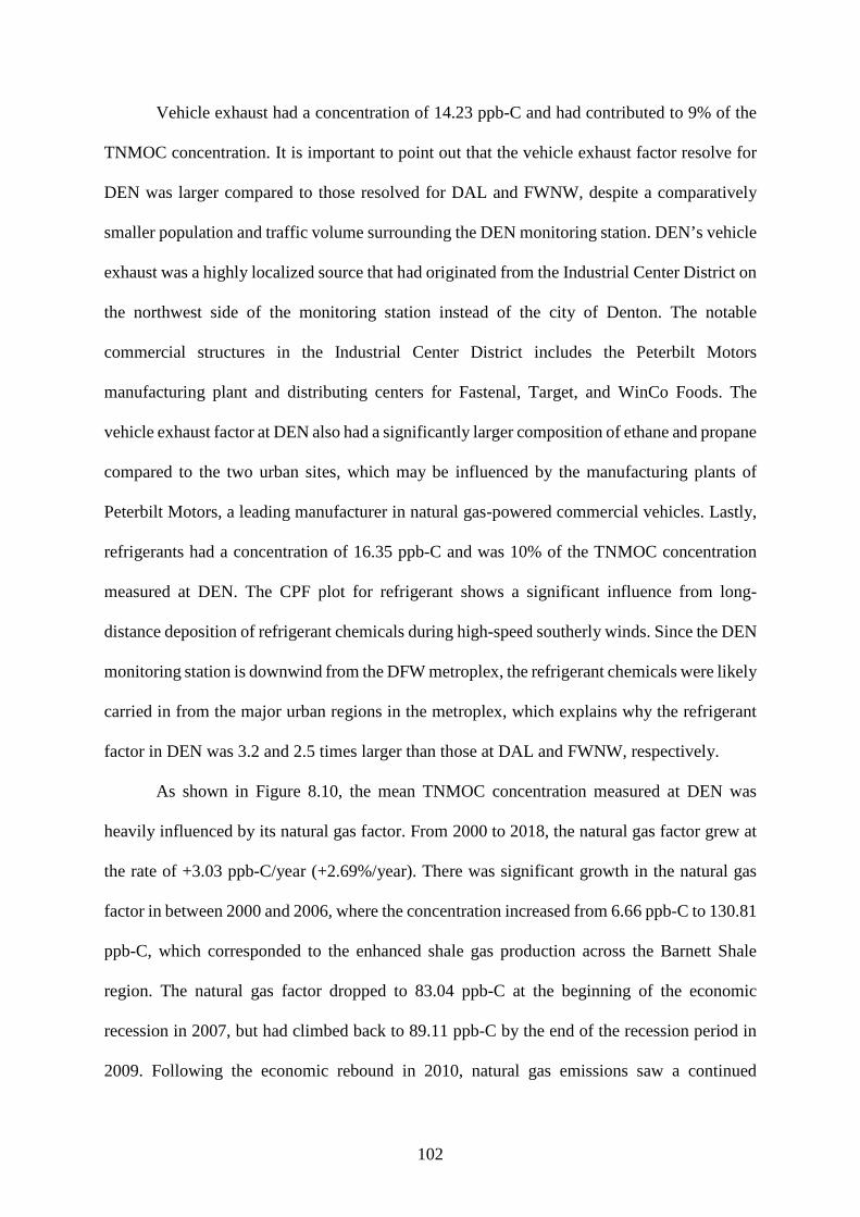
While ozone design values have decreased since 2000, the values measured in Denton

Airport South (DEN), an exurban region in the northwest tip of the Dallas-Fort Worth (DFW)

metroplex, remains above those measured in Dallas Hinton (DAL) and Fort Worth Northwest

(FWNW), two extremely urbanized regions; in addition, all three sites remained in

nonattainment of National Ambient Air Quality Standards (NAAQS) ozone despite reductions

in measured NOx and CO concentrations. The region’s inability to achieve ozone attainment is

tied to its concentration of total non-methane organic compounds (TNMOC). The mean

concentration of TNMOC measured at DAL, FWNW, and DEN between 2000 and 2018 were

67.4 ± 1.51 ppb-C, 89.31 ± 2.12 ppb-C, and 220.69 ± 10.36 ppb-C, respectively. Despite being

the least urbanized site of the three, the TNMOC concentration measured at DEN was over

twice as large as those measured at the other two sites. A factor-based source apportionment

analysis using positive matrix factorization technique showed that natural gas was a major

contributing source factor to the measured TNMOC concentrations at all three sites and the

dominant source factor at DEN. Natural gas accounted for 32%, 40%, and 69% of the measured

TNMOC concentration at DAL, FWNW, and DEN, respectively. The Barnett Shale region, an

active shale gas region adjacent to DFW, is a massive source of unconventional TNMOC

emissions in the region. Also, the ozone formation potential (OFP) of the TNMOC pool in

DEN were overwhelmingly dominated by slow-reacting alkanes emitted from natural gas

sources. While the air pollutant trends and characteristics of an urban airshed can be determined

using long-term ambient air quality measurements, this is difficult in regions with sparse air

quality monitoring. To solve the lack in spatial and temporal datasets in non-urban regions,

various machine learning (ML) algorithms were used to train a computer cluster to predict air

pollutant concentrations. Models built using certain ML algorithms performed significantly

better than others in predicting air pollutants. The model built using the random forest (RF)

algorithm had the lowest error. The performance of the prediction models was satisfactory

when the local emission characteristics at the tested site were like the training site. However,

the performance dropped considerably when tested against sites with significantly different

emission characteristics or with extremely aggregated data points.

ii

Copyright 2020

by

Guo Quan Lim

iii

ACKNOWLEDGMENTS

Firstly, I want to express my most sincere gratitude to my mentor and academic advisor,

Dr. Kuruvilla John, for the continuous support he has provided throughout my master’s and

doctoral degrees. Dr. John’s guidance had helped me tremendously in my research, my writing,

and has helped shaped my attitude towards research and academia. I would also like to thank

Dr. John for always looking out for me outside of my studies and had taught me the importance

of networking with other researchers. I could not have had imagined having a better mentor for

my Ph.D. study.

Besides my advisor, I would like to thank the rest of my thesis committee: Dr. Hamid

Sadat, Dr. Sheldon Shi, Dr. Chetan Tiwari, and Dr. Richard Zhang. I would also like to express

my gratitude to Dr. Saritha Karnae for being a fantastic collaborator in many projects. I also

want to acknowledge the help I had received from Dr. Mahdi Ahmadi, Mr. Constant Marks,

and Ms. Maleeha Matin. They were critical in helping me reach many milestones throughout

my research.

Last but certainly not least, I would like to thank my fiancé, my parents, my sister, and

my family. They were there to show me the love and support I needed for me to get through

my Ph.D. study. They were there to keep me motivated when I couldn’t see the light at the end

of the tunnel. They were there for me to talk to when I was depressed and needed someone the

most. Without them, I would never have made it to the end of this journey.

iv

TABLE OF CONTENTS

Page

ACKNOWLEDGMENTS ....................................................................................................... iii LIST OF TABLES ................................................................................................................... vii LIST OF FIGURES ............................................................................................................... viii CHAPTER 1. INTRODUCTION .............................................................................................. 1 CHAPTER 2. BACKGROUND ................................................................................................ 4 CHAPTER 3. STUDY REGION AND DATA ....................................................................... 10

3.1 Monitoring Sites Equipped with Canister TNMOC Monitors ......................... 11

3.2 Monitoring Sites Equipped with Auto-GC TNMOC Monitors ....................... 12 CHAPTER 4. METHODOLOGY ........................................................................................... 15

4.1 R Programming Language ............................................................................... 15

4.2 Machine Learning Algorithms ......................................................................... 16

4.2.1 Artificial Neural Network .................................................................... 17

4.2.2 Classification and Regression Tree ...................................................... 19

4.2.3 K-Nearest Neighbors ........................................................................... 20

4.2.4 Random Forest ..................................................................................... 21

4.2.5 Support Vector Machines .................................................................... 21

4.3 Positive Matrix Factorization (PMF) ............................................................... 22 CHAPTER 5. SPATIAL AND TEMPORAL CHARACTERISTICS OF AMBIENT ATMOSPHERIC HYDROCARBONS IN AN ACTIVE SHALE GAS REGION IN NORTH TEXAS ..................................................................................................................................... 24

5.1 Spatial Variation in TNMOC Concentration Distribution ............................... 25

5.2 TNMOC Components and Characteristics ...................................................... 28

5.3 Seasonal Trend Analysis .................................................................................. 29

5.4 Spatio-Temporal Distribution of TNMOC ...................................................... 36

5.5 Summary Findings ........................................................................................... 39 CHAPTER 6. A LONG-TERM TREND ANALYSIS OF AIR QUALITY IN THE DALLAS-FORT WORTH AREA: DISCERNING THE IMPACT OF OIL AND GAS EMISSIONS FROM THE BARNETT SHALE ...................................................................... 41

6.1 Oxides of Nitrogen (NOx) ................................................................................ 43

6.2 Carbon Monoxide (CO) ................................................................................... 45

v

6.3 Total Non-Methane Organic Carbon (TNMOC) ............................................. 48

6.3.1 Benzene, Toluene, Ethylbenzene, and Xylene (BTEX) ...................... 51

6.3.2 Natural Gas Production Impacts on TNMOC Levels .......................... 54

6.3.3 Implication on Methane Levels ........................................................... 59

6.4 Ozone ............................................................................................................... 59

6.4.1 TNMOC-NOx-Ozone Relationship ...................................................... 62

6.4.2 Ozone Formation Potential .................................................................. 66

6.5 Summary Findings ........................................................................................... 69 CHAPTER 7. IMPACTS OF SHALE GAS PRODUCTION ON LONG-TERM AMBIENT HYDROCARBON CONCENTRATION IN DENTON, TEXAS .......................................... 71

7.1 Unconventional Gas Development (UGD) in North Texas ............................. 72

7.2 Energy Policies in Texas .................................................................................. 75

7.3 Air Quality in Denton, Texas ........................................................................... 76

7.3.1 Total Non-Methane Organic Carbons (TNMOC) ................................ 76

7.4 Impacts of UGD on TNMOC Concentrations ................................................. 82

7.5 Summary Findings ........................................................................................... 85 CHAPTER 8. SOURCE APPORTIONMENT ANALYSIS OF AMBEINT TNMOC CONCENTRATIONS USING POSITIVE MATRIX FACTORIZATION TECHNIQUE ... 87

8.1 Breakdown of the Measured Hydrocarbon Groups ......................................... 87

8.2 PMF Source Apportionment Analysis ............................................................. 88

8.2.1 Dallas Hinton (DAL) ........................................................................... 89

8.2.2 Fort Worth Northwest (FWNW) .......................................................... 94

8.2.3 Denton Airport South (DEN) ............................................................... 98

8.3 Summary Findings ......................................................................................... 103 CHAPTER 9. ADOPTING MACHINE LEARNING TECHNIQUES FOR AIR QUALITY DATA ANALYSIS ................................................................................................................ 105

9.1 Training and Validating Dataset Variables .................................................... 105

9.2 Simple vs Ensemble ML Model .................................................................... 106

9.3 Identifying the Ideal Training Dataset Sample Size ...................................... 107

1.1. Performance of ML models ........................................................................... 108

9.3.1 Artificial Neural Network (ANN) ...................................................... 110

9.3.2 Classification and Regression Tree (CaRT) ...................................... 110

9.3.3 k-Nearest Neighbor (kNN) ................................................................ 111

9.3.4 Random Forest (RF) .......................................................................... 112

9.3.5 Support Vector Machine (SVM) ........................................................ 113

vi

9.3.6 ML Model Performance Comparison ................................................ 115

9.4 Testing the ML Models against Photochemical Models................................ 117

9.5 Testing the ML Models for Various Locations .............................................. 122

9.6 Summary Findings ......................................................................................... 127 CHAPTER 10. CONCLUSION AND RECOMMENDATIONS ......................................... 129

10.1 Conclusion ..................................................................................................... 129

10.2 Recommendations .......................................................................................... 131 APPENDIX A. SUPPLEMENTAL FIGURES ..................................................................... 133 APPENDIX B. SUPPLEMENTAL TABLES ....................................................................... 143 REFERENCES ...................................................................................................................... 154

vii

LIST OF TABLES

Page

Table 5.1: Summary of TNMOC and hydrocarbon groups (ppb-C). ...................................... 27

Table 6.1: National Emissions Inventory (NEI) for Criteria and Hazardous Air Pollutants by 60 Emissions Inventory System (EIS) emission sectors of VOC, CO, and NOx (tons) [121]. 42

Table 6.2: The Pearson's R-value between the (i) OFP of reactive groups and (ii) OFP of alkanes with ozone values at Dallas Hinton, Fort Worth Northwest, and Denton Airport South. ....................................................................................................................................... 69

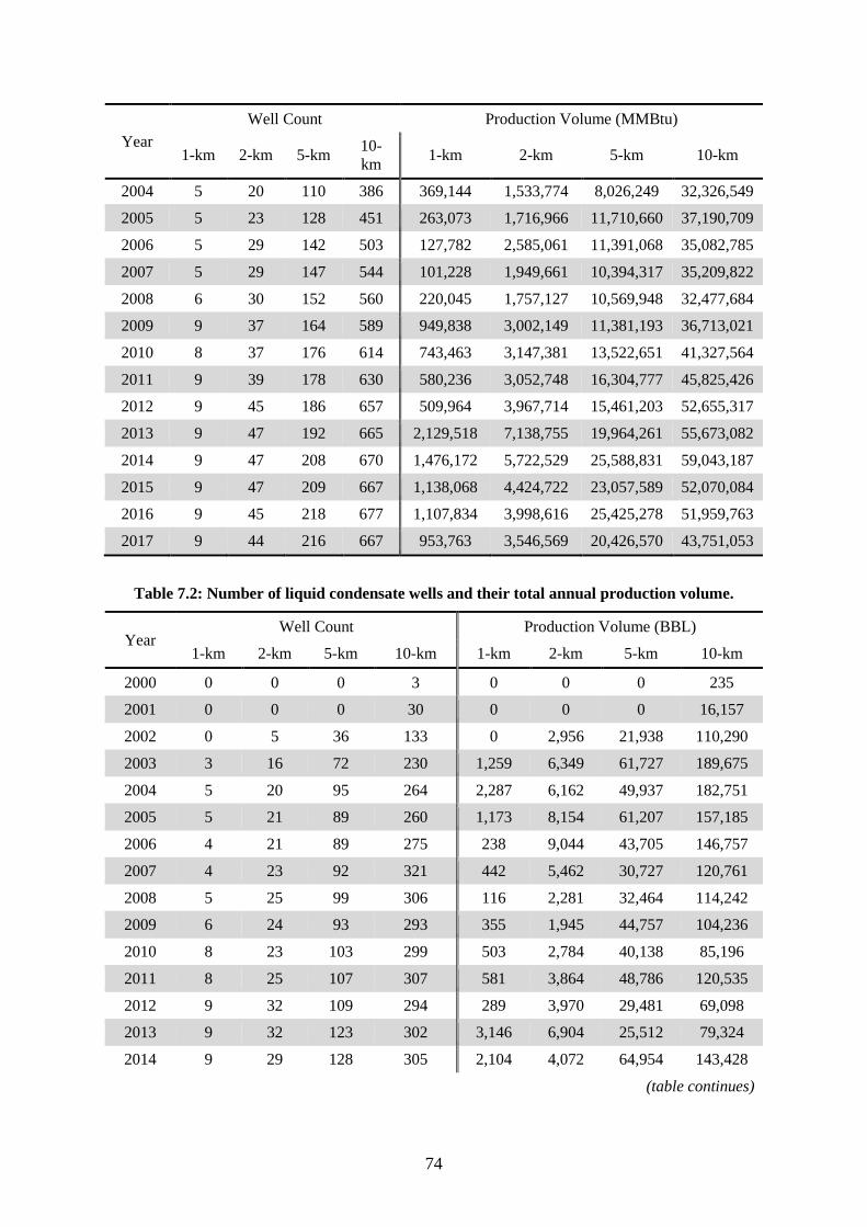
Table 7.1: Number of natural gas wells and their total annual production volume. ................ 73

Table 7.2: Number of liquid condensate wells and their total annual production volume. ..... 74

Table 7.3: Mean TNMOC concentration measured and the average change in annual TNMOC during the 2000-2006, 2007-2009, 2010-2013, and 2014-2017 periods. ................. 77

Table 8.1: Resolved PMF sources factor profile (ppb-C, %) and their respective key species................................................................................................................................................... 89

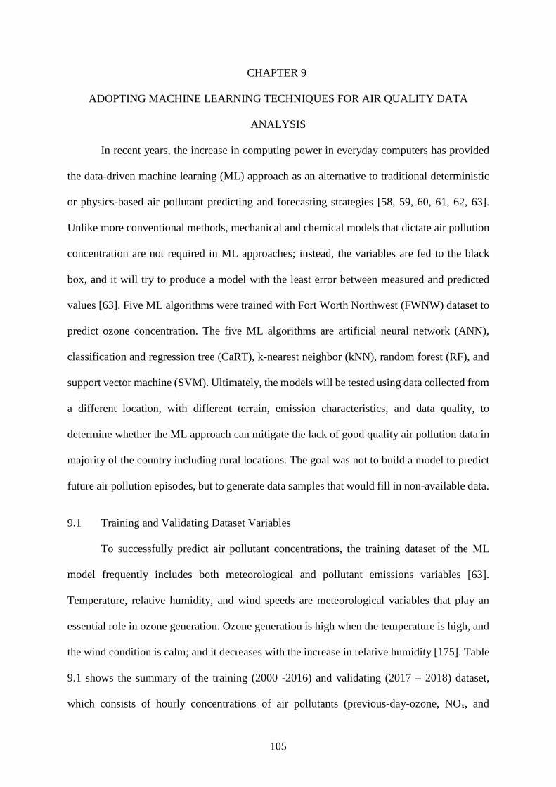
Table 9.1: Summary of the training (2000 – 2016) and validating (2017 – 2018) datasets. . 106

Table 9.2: The performance of the ML model using different training dataset sizes. ........... 108

Table 9.3: Training dataset variable importance to the RF model. ........................................ 113

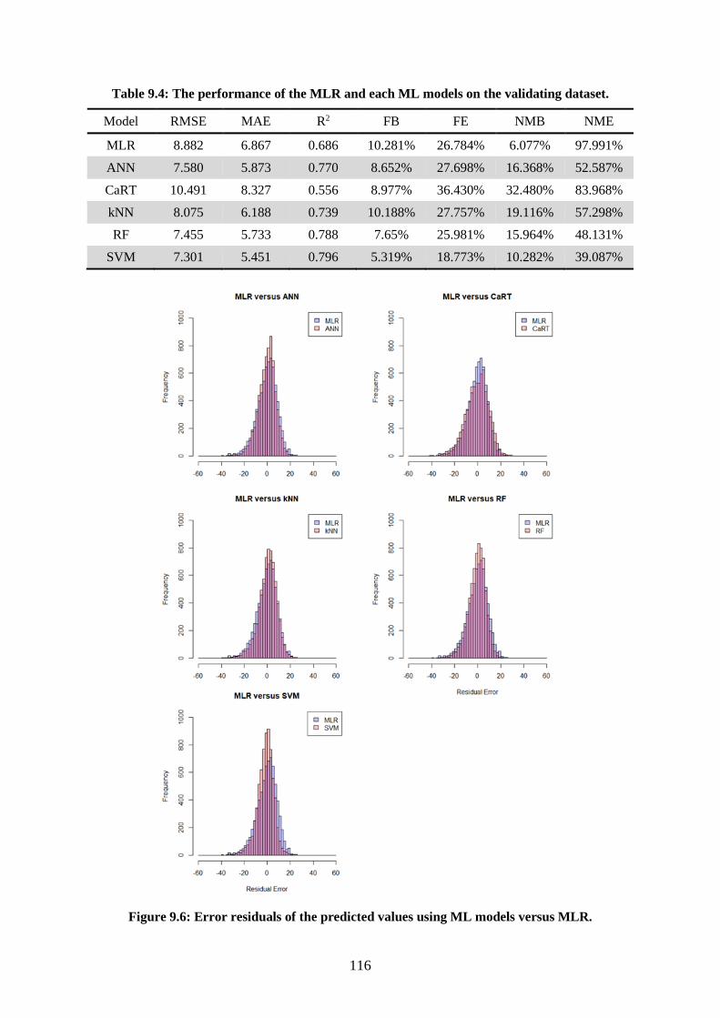
Table 9.4: The performance of the MLR and each ML models on the validating dataset. ... 116

Table 9.5: The performance of each ML model in comparison to TCEQ’s 2012 base case ozone on CAMx. .................................................................................................................... 118

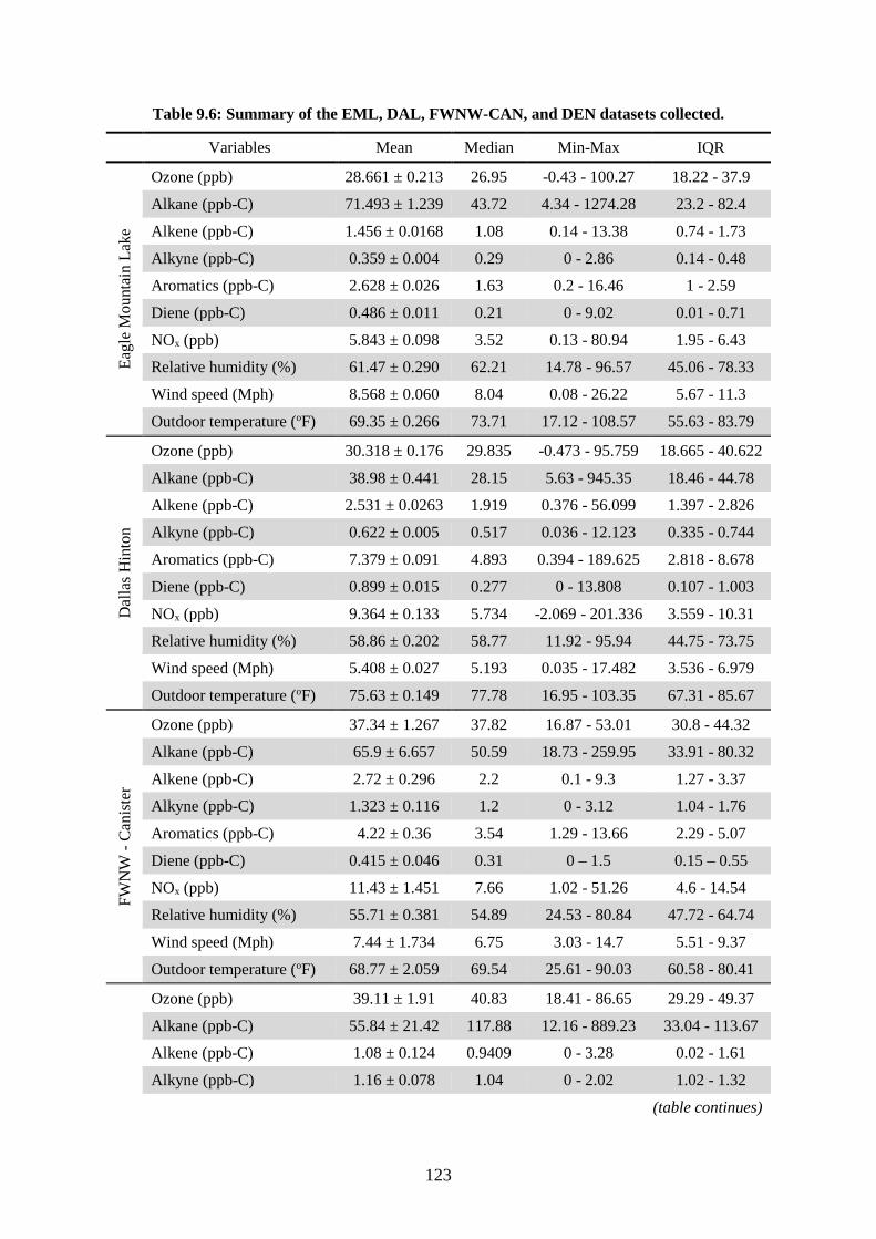
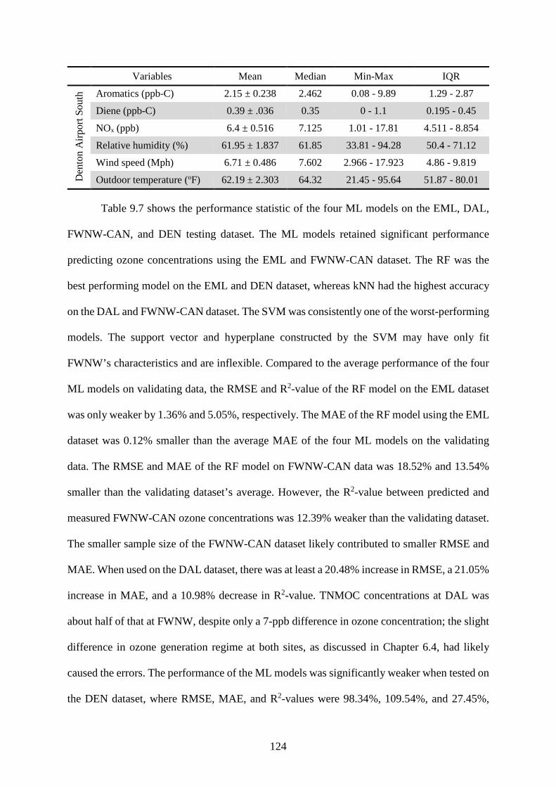
Table 9.6: Summary of the EML, DAL, FWNW-CAN, and DEN datasets collected. ......... 123

Table 9.7: Performance of the ANN, kNN, RF, and SVM models on the EML, DAL, FWNW-CAN, and DEN testing datasets. .............................................................................. 125

viii

LIST OF FIGURES

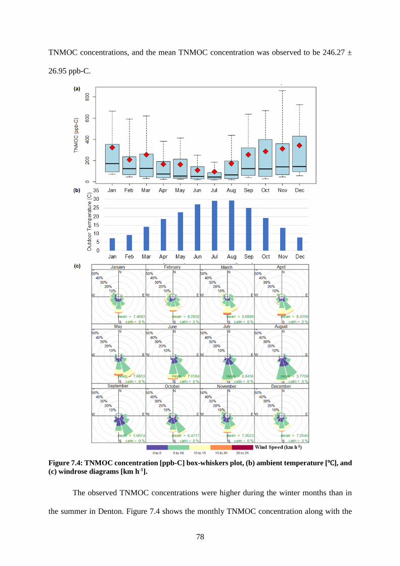
Page

Figure 3.1: Map of SUMMA canister sites along with active oil and gas wells. .................... 12

Figure 3.2: Map of Auto-GC monitoring station along with active oil and gas wells. ............ 13

Figure 4.1: Framework of an artificial neural network (ANN) [80]. ....................................... 18

Figure 5.1: Wind rose diagrams for C1007, C13, C75, C88, and C1013: 2011-2015. ............ 25

Figure 5.2: Annual trend of TNMOC (ppb-C) concentrations measured at C1007, C13, C75, C1013, and C88 from 2011 to 2015......................................................................................... 26

Figure 5.3: Comparison between urban and non-urban site TNMOC concentration, alkane/TNMOC, alkene/TNMOC, alkyne/TNMOC, aromatic/TNMOC, and isoprene/TNMOC concentration ratio. .................................................................................... 29

Figure 5.4: Seasonal variation of (a) TNMOC (ppb-C) and alkane/TNMOC concentration ratio, (b) alkene/TNMOC and alkyne/TNMOC concentration ratio, and (c) aromatics/TNMOC and isoprene/TNMOC concentration ratio. ............................................. 33

Figure 5.5: Conditional Bivariate Probability Function plot for 50th to 75th percentile, 75th to 95th percentile, and >95th percentile at C1007 and C13. ........................................................ 37

Figure 5.6: Conditional Bivariate Probability Function plot for 50th to 75th percentile, 75th to 95th percentile, and >95th percentile at C75, C1013, and C88. .............................................. 38

Figure 6.1: Trends of NOx concentration (ppb) at Dallas Hinton, Fort Worth Northwest, and Denton Airport South. .............................................................................................................. 44

Figure 6.2: Trends of CO concentration (ppm) at Dallas Hinton and Fort Worth Northwest. 46

Figure 6.3: Trends of TNMOC concentration (ppb-C) at Dallas Hinton, Fort Worth Northwest, and Denton Airport South. .................................................................................... 48

Figure 6.4: Trend of median BTEX concentrations (ppb-C) in Dallas Hinton, Fort Worth Northwest, and Denton Airport South. .................................................................................... 52

Figure 6.5: Number of active gas wells within 5-km from Fort Worth Northwest and Denton Airport South along with the total natural gas production volume (MMBtu). ........................ 54

Figure 6.6: Trends of acetylene/TNMOC, ethane/TNMOC, CO/TNMOC, and NOx/TNMOC concentration ratio. .................................................................................................................. 56

Figure 6.7: Relationship between isopentane and n-pentane at Dallas Hinton, Fort Worth Northwest, and Denton Airport South. .................................................................................... 57

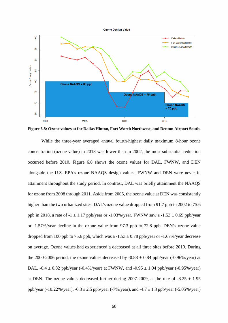
Figure 6.8: Ozone values at for Dallas Hinton, Fort Worth Northwest, and Denton Airport South. ....................................................................................................................................... 60

ix

Figure 6.9: Trends of ozone concentration (ppb) at Dallas Hinton, Fort Worth Northwest, and Denton Airport South. .............................................................................................................. 61

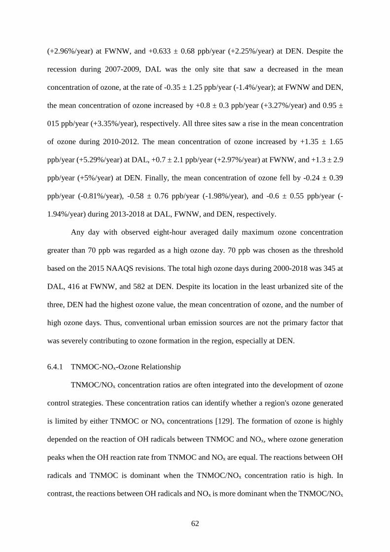
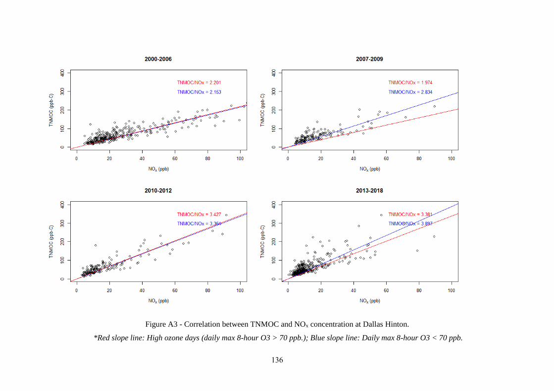
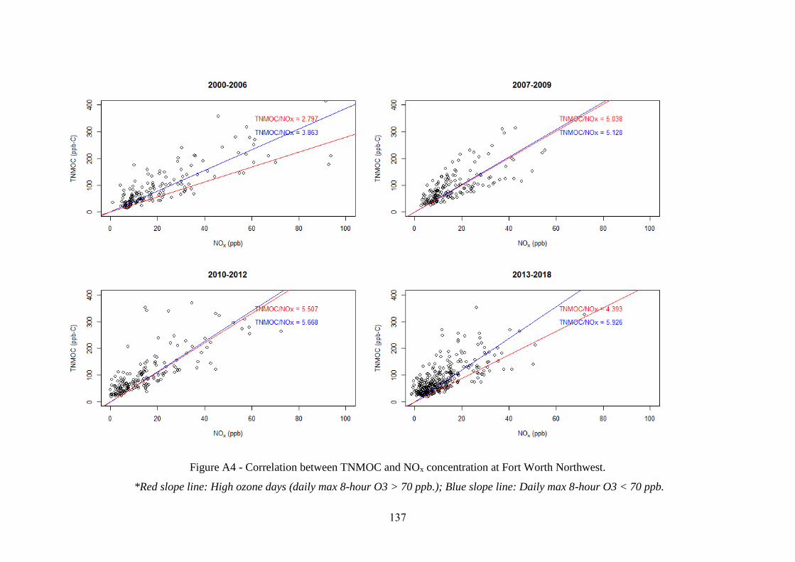
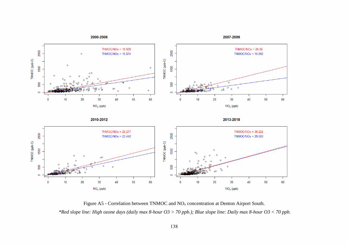
Figure 6.10: Relationship between ozone concentration and the corresponding TNMOC/NOx ratios. ........................................................................................................................................ 63

Figure 6.11: Relationship between ozone formation potential (OFP) with the TNMOC concentration by hydrocarbon groups. ..................................................................................... 67

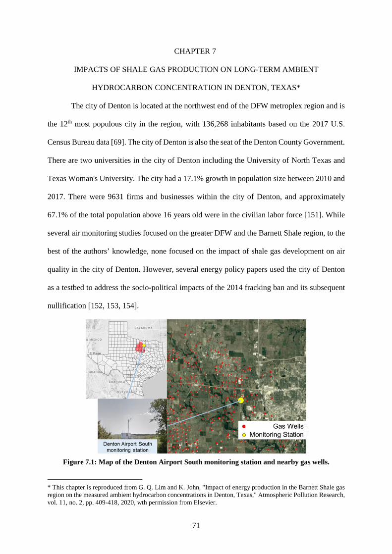
Figure 7.1: Map of the Denton Airport South monitoring station and nearby gas wells. ........ 71

Figure 7.2: Barnett Shale natural gas production (MMBtu/day), new gas well permit issued, and average natural gas spot price ($/MMBtu). ....................................................................... 73

Figure 7.3: TNMOC concentration (ppb-C) timeseries plot for 2000 – 2017. ........................ 77

Figure 7.4: TNMOC concentration [ppb-C] box-whiskers plot, (b) ambient temperature [℃], and (c) windrose diagrams [km h-1]. ........................................................................................ 78

Figure 7.5: (a) Alkane/TNMOC, (b) alkene/TNMOC, and (c) aromatics/TNMOC concentration ratios box-whiskers plots................................................................................... 79

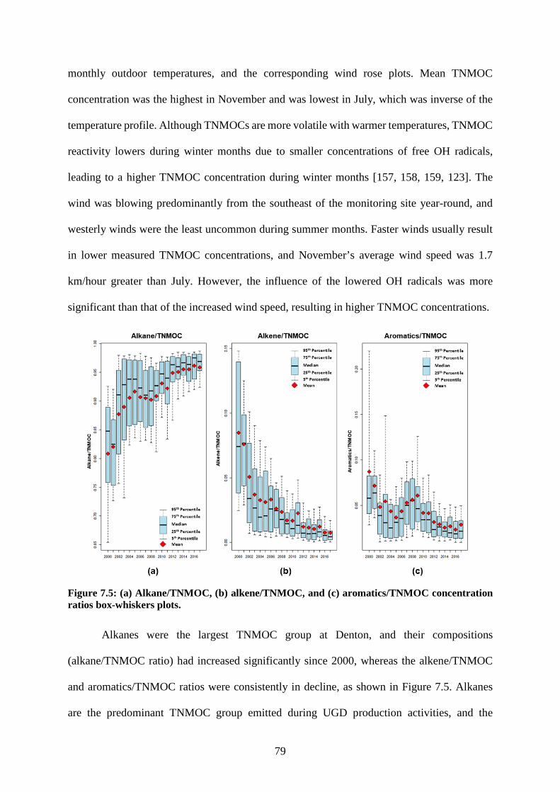
Figure 7.6: Alkanes (ethane, propane, and n-butane), alkenes, and alkynes (acetylene, ethylene, and propylene), and aromatics (benzene, toluene, ethylbenzene, and xylene) concentrations from 2000 to 2017. .......................................................................................... 80

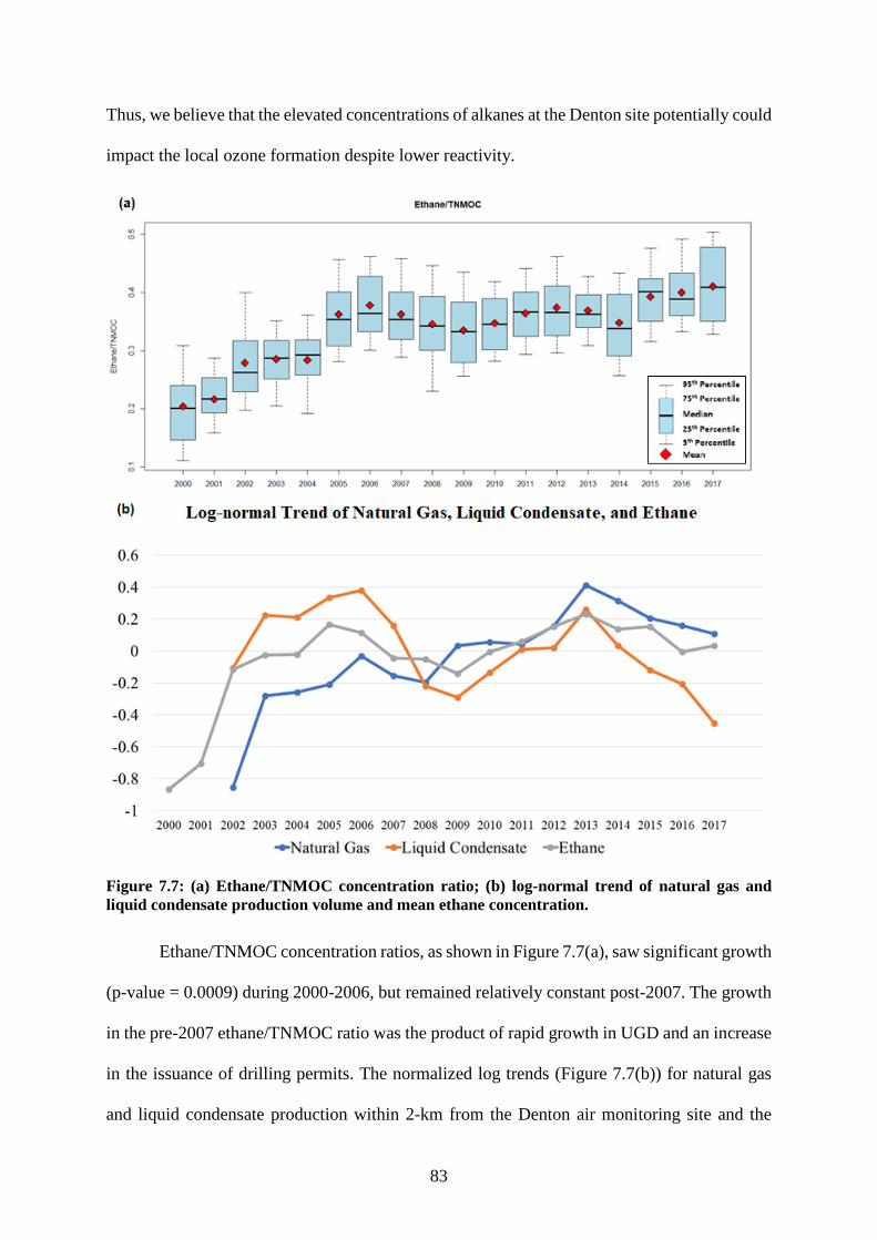
Figure 7.7: (a) Ethane/TNMOC concentration ratio; (b) log-normal trend of natural gas and liquid condensate production volume and mean ethane concentration. .................................. 83

Figure 7.8: (a) Location of natural gas wells overlaid with total production volume contour [MMBtu]; (b) location of liquid condensate facilities overlaid with total production volume contour [BBL]; and (c) bivariate polar plot for measured ethane concentrations [ppb-C]. ..... 84

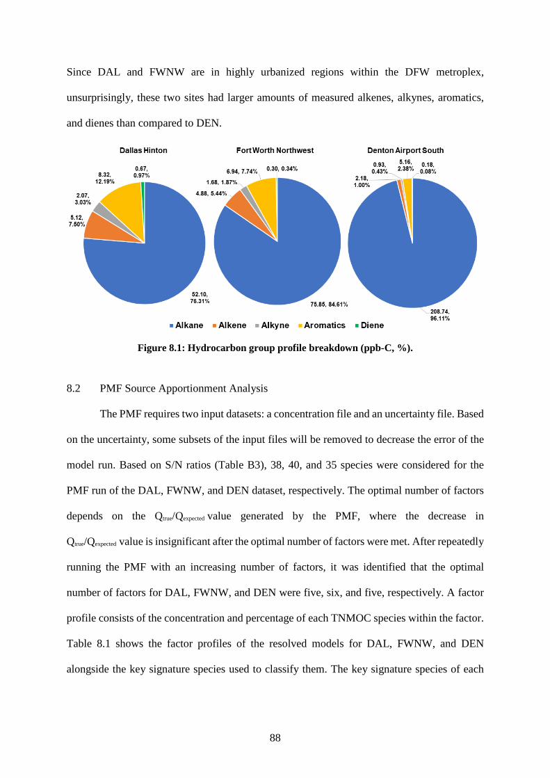
Figure 8.1: Hydrocarbon group profile breakdown (ppb-C, %). ............................................. 88

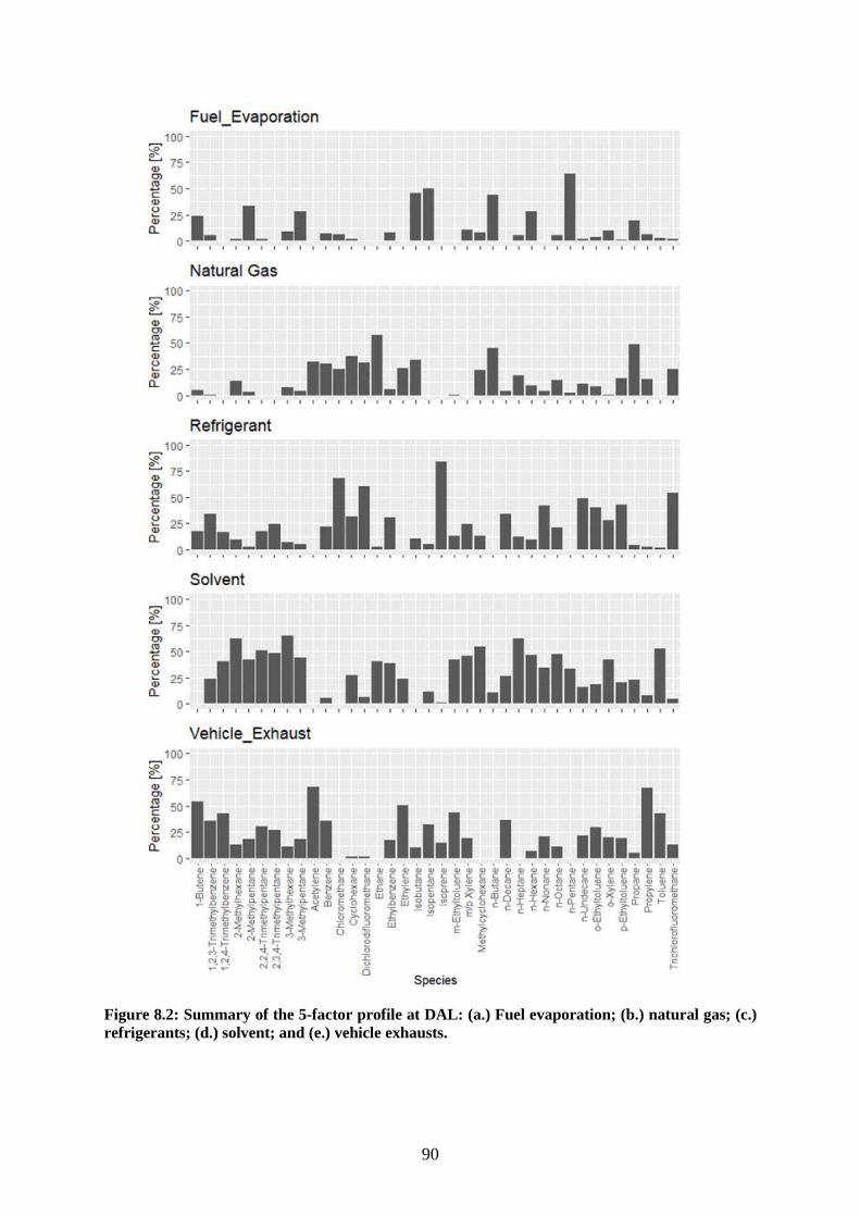
Figure 8.2: Summary of the 5-factor profile at DAL: (a.) Fuel evaporation; (b.) natural gas; (c.) refrigerants; (d.) solvent; and (e.) vehicle exhausts. .......................................................... 90

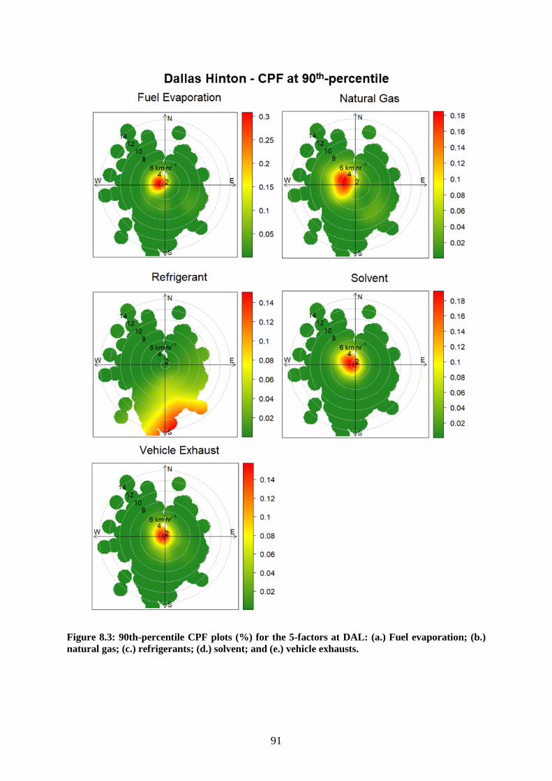
Figure 8.3: 90th-percentile CPF plots (%) for the 5-factors at DAL: (a.) Fuel evaporation; (b.) natural gas; (c.) refrigerants; (d.) solvent; and (e.) vehicle exhausts. ...................................... 91

Figure 8.4: Annual variation in the mean concentration of the 5-factors at DAL. .................. 93

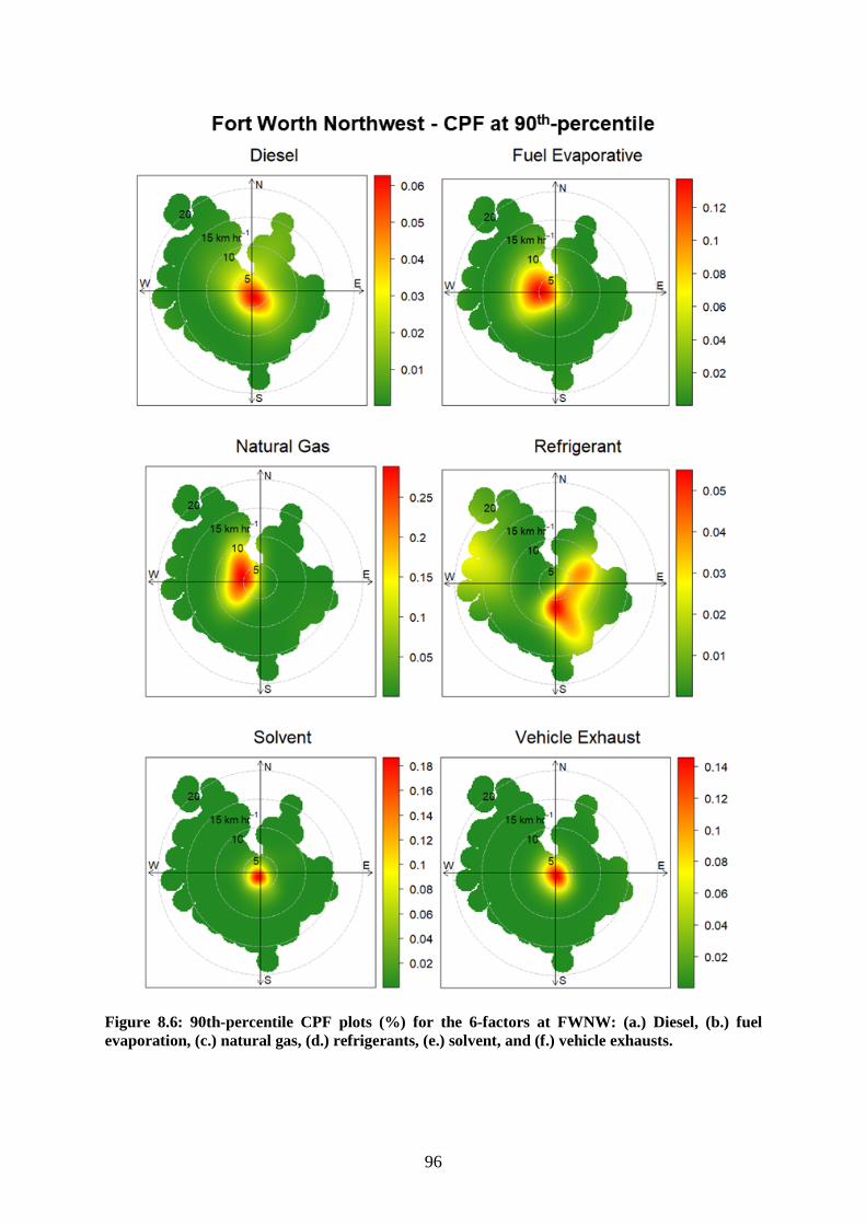
Figure 8.5: Summary of the 6-factor profile at FWNW: (a.) Diesel, (b.) fuel evaporation, (c.) natural gas, (d.) refrigerants, (e.) solvent, and (f.) vehicle exhausts. ....................................... 95

Figure 8.6: 90th-percentile CPF plots (%) for the 6-factors at FWNW: (a.) Diesel, (b.) fuel evaporation, (c.) natural gas, (d.) refrigerants, (e.) solvent, and (f.) vehicle exhausts. ............ 96

Figure 8.7: Annual variation in the mean concentration of the 6-factors at FWNW............... 98

x

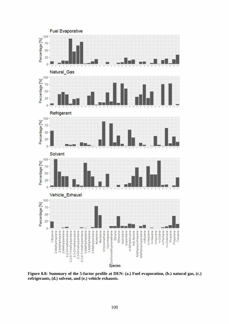
Figure 8.8: Summary of the 5-factor profile at DEN: (a.) Fuel evaporation, (b.) natural gas, (c.) refrigerants, (d.) solvent, and (e.) vehicle exhausts. ........................................................ 100

Figure 8.9: 90th-percentile CPF plots (%) for the 5-factors at DEN: (a.) Fuel evaporation, (b.) natural gas, (c.) refrigerants, (d.) solvent, and (e.) vehicle exhausts. .................................... 101

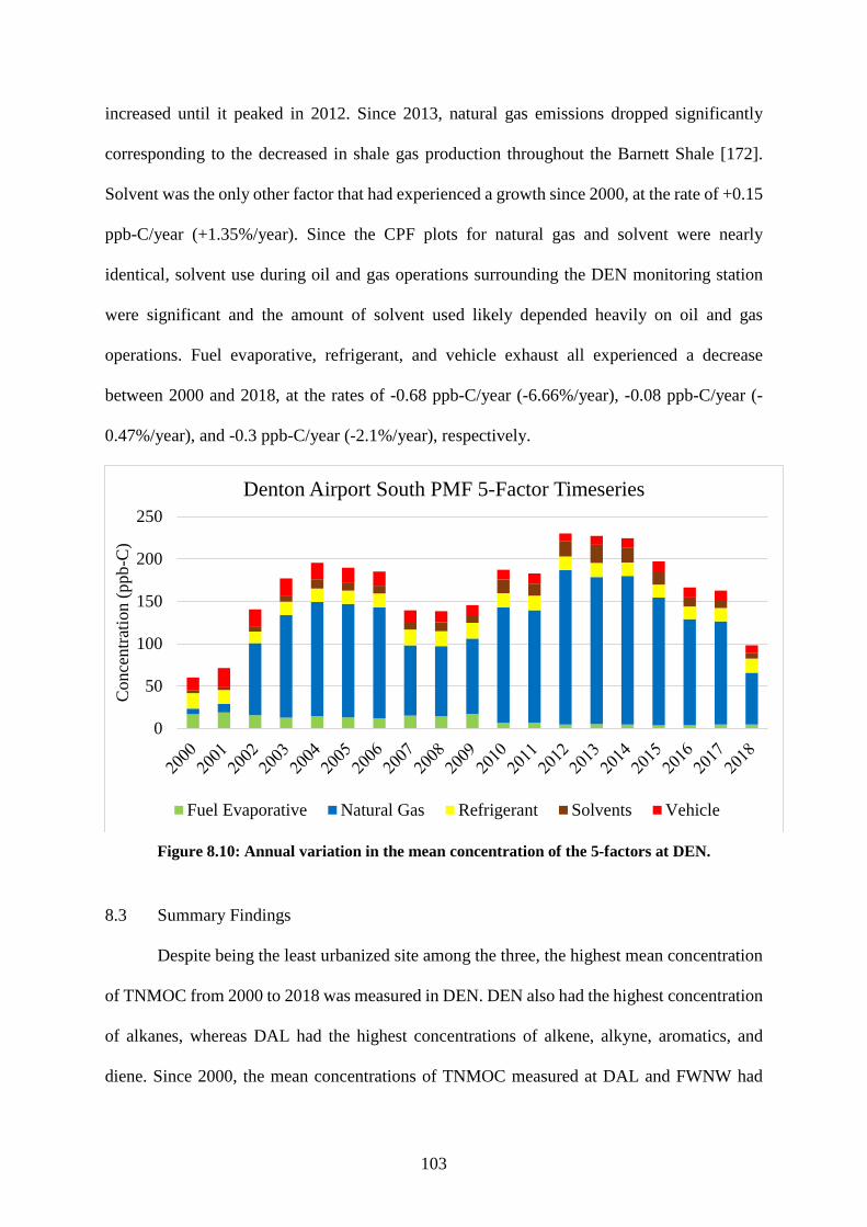
Figure 8.10: Annual variation in the mean concentration of the 5-factors at DEN. .............. 103

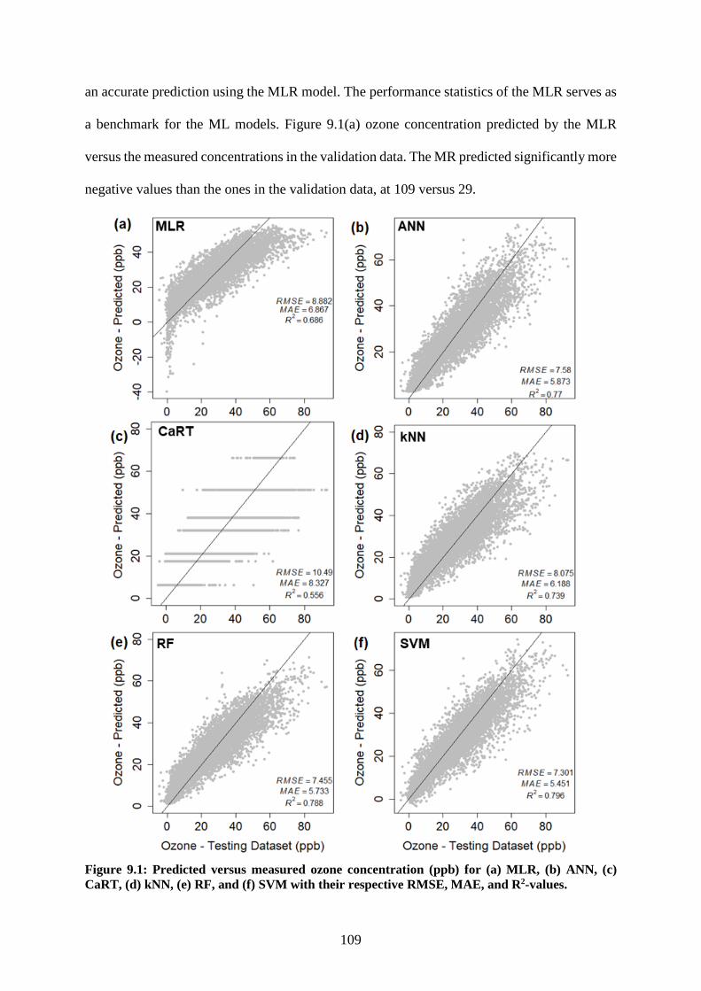
Figure 9.1: Predicted versus measured ozone concentration (ppb) for (a) MLR, (b) ANN, (c) CaRT, (d) kNN, (e) RF, and (f) SVM with their respective RMSE, MAE, and R2-values. .. 109

Figure 9.2: Relative error versus cp and tree size. ................................................................. 111

Figure 9.3: Pruned regression decision tree. .......................................................................... 111

Figure 9.4: Number of k-values versus RMSE for the kNN regression. ............................... 112

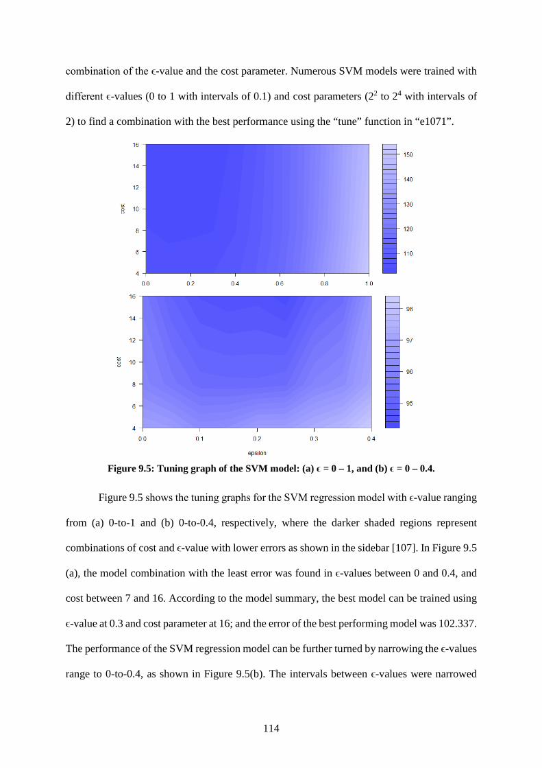
Figure 9.5: Tuning graph of the SVM model: (a) ϵ = 0 – 1, and (b) ϵ = 0 – 0.4. ................... 114

Figure 9.6: Error residuals of the predicted values using ML models versus MLR. ............. 116

Figure 9.7: Observed versus predicted ozone concentration (ppb) using the TCEQ photochemical model and ML models. .................................................................................. 120

Figure 9.8: Daily averaged observed versus predicted ozone concentration (ppb) using the TCEQ photochemical model and ML models. ...................................................................... 121

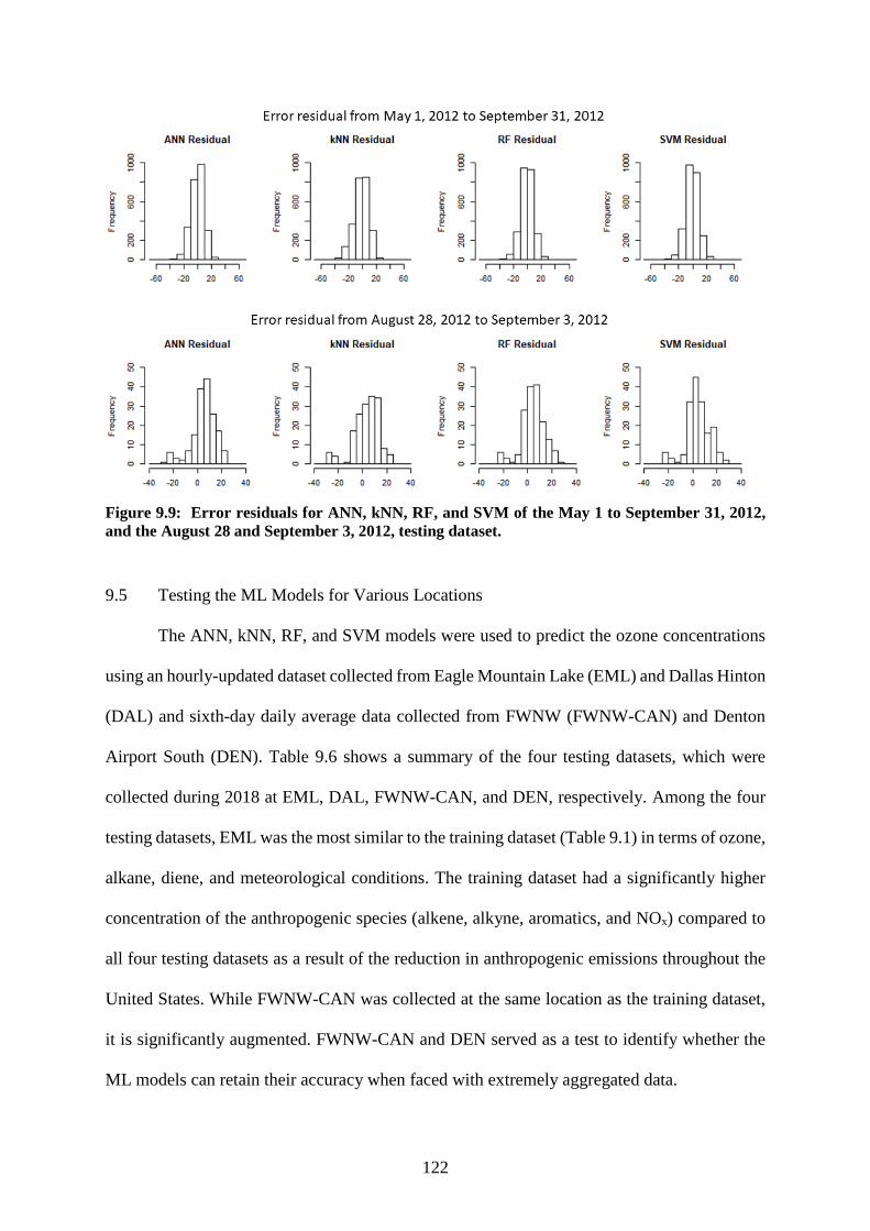
Figure 9.9: Error residuals for ANN, kNN, RF, and SVM of the May 1 to September 31, 2012, and the August 28 and September 3, 2012, testing dataset. ......................................... 122

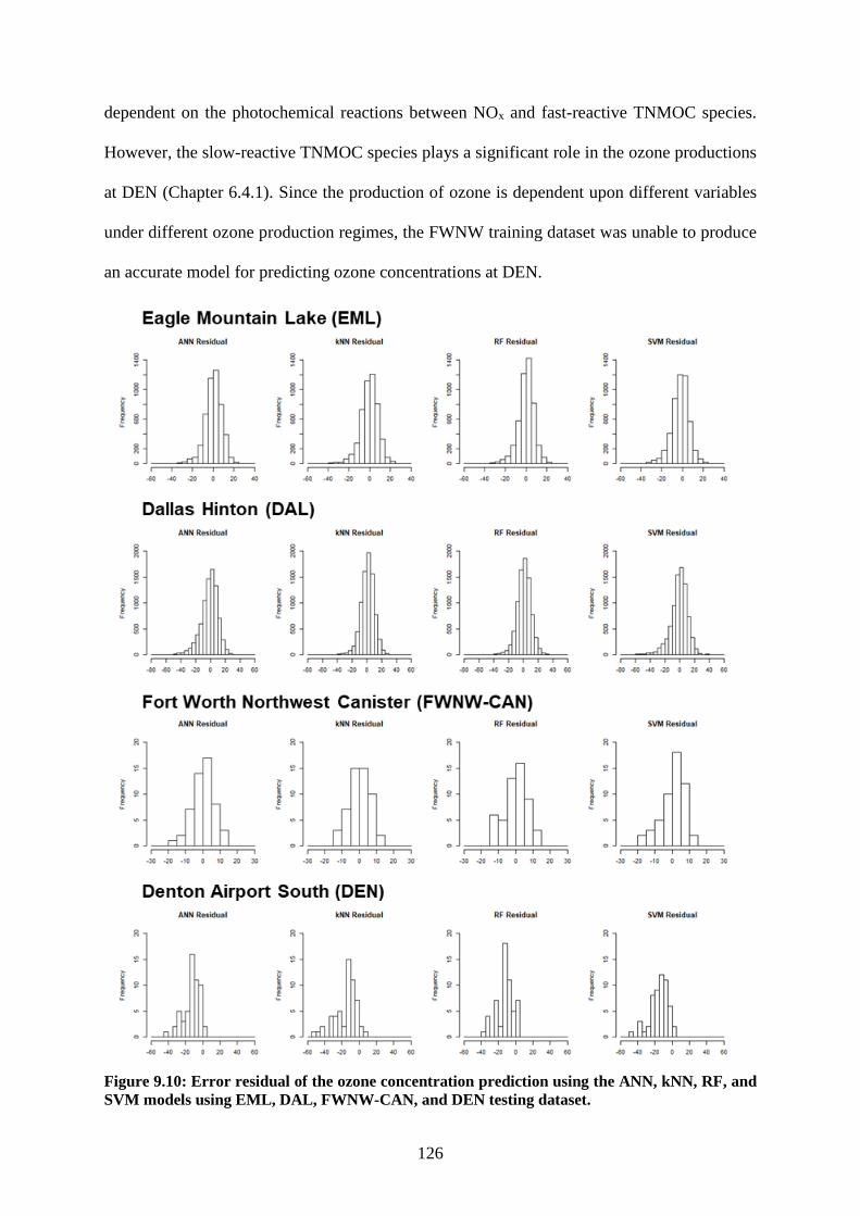
Figure 9.10: Error residual of the ozone concentration prediction using the ANN, kNN, RF, and SVM models using EML, DAL, FWNW-CAN, and DEN testing dataset. .................... 126

1

CHAPTER 1

INTRODUCTION

The Dallas – Fort Worth (DFW) metroplex region is one of the largest metropolitan

regions in the United States [1] and had seen a massive increase in oil and gas production

activities in the past two decades from the Barnett Shale region [2]. The expansion in shale gas

production had drastically increased emissions from non-conventional shale gas sources, and

this threatens the environment and the people living in the metroplex. Shale gas production is

a significant source of volatile organic compounds (VOC), a precursor for ground-level ozone

formation. Ozone is a criteria pollutant that can cause severe health issues, especially in the

sensitive group of young children, older adults, and those with existing lung conditions.

Overexposure to ozone leads to several health problems such as chronic obstructive pulmonary

disease (COPD), shortness of breath, and other respiratory ailments [3]. While the ozone levels

in DFW had shown improvements since 2000, ten of the twelve DFW counties still consistently

fail to comply with the design value designated by the United States Environmental Protection

Agency (EPA) through the Clean Air Act’s National Ambient Air Quality Standard (NAAQS)

[4]. Denton, Johnson, Tarrant, and Wise are the leading shale gas producing counties in the

Barnett Shale, and all four counties consistently fail to meet ozone attainment under the

NAAQS.

The objective of this work is to study the long-term impact on DFW air quality due to

elevated shale gas production over the past two decades. While the air quality impacts of shale

gas are well-documented, relatively few studies truly focus on the Barnett Shale and its impact

on the DFW metroplex region. The available literature on the subject does not provide a

consensus on whether the increased shale gas production in the neighboring Barnett Shale had

any significant impact on DFW’s air quality [5, 6, 7]. To the best of the author’s knowledge,

this dissertation is the most comprehensive work on long-term VOC, oxides of nitrogen (NOx),

2

carbon monoxide (CO), and ozone concentrations measured in DFW. Data mining and data

analysis techniques were also implemented to correlate unconventional shale gas production

and local VOC concentrations. However, the lack of consistent air quality data from non-urban

regions within the Barnett Shale severely hinders the progress of understanding the full extent

of the shale gas production’s impacts. While traditional photochemical models can simulate air

pollutant concentration and deposition at these non-urban/rural regions, the scale of these

simulation predictions are very coarse and simulated by using specific air pollution episodes

[8]. This dissertation describes an attempt to incorporate machine learning (ML) algorithms in

air pollutant concentration prediction models. A model can be trained using regression-based

ML algorithms to predict the non-linear ozone concentration in remote regions using the robust

data collected from the DFW metroplex used as the training set.

This dissertation covers the following issues:

(i) Perform data mining and analysis to characterize the air quality trends observed in the DFW metroplex between 2000 and 2019.

(ii) Identify the potential impacts of unconventional shale gas development in the Barnett Shale on local and regional air quality.

(iii) Perform source apportionment analysis to identify major emission sources contributing to air pollutant concentrations.

(iv) Compare the performance of various ML algorithms on their ability to predict non-linear ozone concentrations and whether the ML models are comparable to more traditional air quality simulation models.

Chapter 1 of this report introduces this study and states the objectives and outlines the

work performed. Chapter 2 highlights the background and provides a detailed literature review

relevant to this study. Chapter 3 details the descriptions of the study area covering the DFW

metroplex, the air quality monitoring stations, and the data used in this study. Chapter 4

summarizes the methods and techniques used in this dissertation. The results and discussions

of each part of this study are available from Chapters 5 through 9. Chapter 5 describes the study

of short-term VOC concentrations collected from five monitoring stations in DFW. Chapter 6

3

describes a long-term analysis of various air pollutants from three DFW monitoring stations.

In Chapter 7, the impacts of unconventional gas development on the VOC concentrations in

Denton, Texas, was studied. Chapter 8 details a source apportionment analysis using positive

matrix factorization (PMF) method on long-term VOC concentration data collected in DFW.

Chapter 9 describes a comparative study of various ozone prediction models trained using ML

algorithms, their performance against traditional photochemical models, and their adaptability

using non-local data. The conclusion of this study and recommendations for future work are

provided in Chapter 10.

The contents of Chapter 5 and Chapter 7 have been published in peer reviewed journals

such as Science of the Total Environment [9] and Atmospheric Pollution Research [10],

respectively. As of the writing of this dissertation report, a portion of the contents discussed in

Chapter 6 was submitted for publication in Atmospheric Pollution Research. Additional

manuscripts from Chapters 8 and 9 are currently being developed for journal article

submission.

4

CHAPTER 2

BACKGROUND

Energy production is predicted to rise in the upcoming decades to supply the growing

demands from rapid urbanization and industrialization of many regions across the world. An

increasing number of countries, including China and certain parts of Europe, sees natural gas

as a cleaner alternative to coal due to significantly lower oxides of nitrogen (NOx), carbon

dioxide (CO2), and sulfur dioxide (SO2) emissions [11, 12, 13, 14, 15]. The Energy Information

Administration (EIA) has estimated a rapid growth in natural gas production by 7% per year

(+7%/year) between 2018 and 2020, followed by a +1%/year increase through 2050. The EIA

estimated the natural gas production by 2029 to be at 22.4 MMBtu/day from 13.5 MMBtu/day

in 2018, and further development in shale gas resources is required to support this growth [16].

Shale gas is natural gas trapped under shale formation and is an increasingly valuable

energy resource in the United States. Through advancements in hydraulic fracturing and

horizontal drilling technologies [17], significantly harvesting shale gas is now possible, and the

access to shale gas has increased the world’s available natural gas resources [18]. Shale gas

production in the United States accounted for only 5% of total dry gas production in 2004; in

2015, shale gas production was 56% of total dry gas production in the United States [15]. In

2017, the United States Energy Information Administration (EIA) estimated about 62% of the

total dry natural gas produced in the United States was from shale resources, which totals

approximately 16.9 trillion cubic feet of dry natural gas. [19]. The International Energy

Agency (IEA) has predicted the natural gas demand to increase by 42% by 2040 [18].

Environmental health controversies often surround shale gas extraction and production.

Countless factors, from gas well preparation to gas processing, play a crucial role in increasing

pollutant concentrations. The increased shale gas production activities around the U.S. are

negatively affecting many local neighborhoods and communities. Contamination of water

5

resources, ambient air pollution, light and noise pollution, and seismic activities are among the

most prominent environmental issues caused by shale gas production [20, 21]. Also, the

extraction processes cause a significant drain on water resources as 12 to 20 million liters of

water on average are required to produce a single horizontal well [22, 23]. Commonly used

hydraulic fracturing liquids also contain toxic and carcinogenic chemicals that can affect

human health [24]. Ground-water pollution from faulty seals in gas wells are not uncommon,

and hydraulic fracturing liquid often contains toxic and carcinogenic elements [24, 25].

Regions with a large amount of shale gas production often have heightened the risk of seismic

events, as fracking operations may lead to low magnitude earthquakes and gas well blowouts

[26]. Shale gas operations tend to generate a lot of noise and light pollution [27]. The massive

deforestation during shale gas operations also endangers the natural habitats of wildlife [28].

Rapid development in the Marcellus Shale, a shale formation that underlies parts of

Ohio, West Virginia, Pennsylvania, and New York, caused an estimated $7.2 million to $32

million in air quality damages. The population living close to active gas well regions is often

at elevated health risks [29]. Shale gas productions in the United States tend to stay away from

densely populated areas as much as possible. However, this was possible because the

population density in the United States is considerably lower than in parts of Europe and China.

Increased shale gas development in more densely populated regions may lead to endangerment

of the population, especially in regions lacking a proper legal framework to protect both people

and the environment [23].

Shale gas operations emit a lot of air pollutants and greenhouse gases (GHG) into the

atmosphere, which contributes to global warming and threatens human health [30, 31, 32].

Composition of natural gas emissions varies, and they usually contain 88% methane, 5%

ethane, 2% propane, 1.4% carbon dioxide, 1.2% nitrogen, and 0.6% n-butane [33]. Methane is

a potent GHG emitted during shale gas operations. Methane's hundred-year global warming

6

potential is 28 times that of CO2 [34]. An estimated 3.6% to 7.9% of shale gas produced escapes

into the atmosphere as fugitive methane. Fugitive methane emissions escape through leaks

from equipment during gas well completion, transportation, storage, and distribution [11]. In a

typical shale gas operation, between 1.3% and 1.9% of the natural gas produced are lost to the

atmosphere as fugitive methane [32]. 49 of the 50 sampling events in a study of ambient

hydrocarbon analysis in North Texas’s Barnett Shale observed methane concentrations above

the laboratory detection limit, and the concentrations in the region were higher than the reported

urban background concentration of 1.8 to 2 ppm [7]. Direct exposure to the hydrocarbons

released from petrochemical operations is known to be damaging to human health [29].

The U.S. EPA has listed: (i) completions with fracking, (ii) pneumatic vents, (iii)

injection pumps, (iv) leakage from equipment, (v) workovers without fracking, (vi) liquid

unloading, (vii) condensate tanks, (viii) gas engines, (ix) dehydrator vents, (x) reciprocating

compressors, (xi)drilling of wells, (xii) well blowouts, and (xiii) coal beds as dominant active

sources of methane emissions in most common shale gas production locations [30, 31]. During

the development phase, major VOC sources include completion vents and condensate tanks,

whereas drill rigs, fracturing pumps, and traffic emissions from trucks are minor VOC sources.

Compressor stations are major VOC sources, while wellhead compressors, heaters, blowdown

vents, and pneumatics are minor VOC sources during the production phase [35].

Litovitz et al. [36] found Pennsylvania’s Marcellus Shale had gas well emissions that

were ten times larger than associated diesel and road dust emissions. They identified shale gas

production to be an incredibly damaging factor to regional air quality. Volatile organic

compounds (VOC) are a group of carbon-based chemicals emitted from either anthropogenic

or biogenic sources. The U.S. EPA defines VOCs as carbon compounds that react

photochemically in the atmosphere, which also includes compounds with low photochemical

reactivity, such as methane and ethane, but excludes carbon monoxide (CO), CO2, carbonic

7

acid, and carbonates [37]. Many VOC species are considered air toxins, and overexposure to

VOC can lead to irritations, nausea, headaches, and damages to the nervous system, kidney, or

liver [38]. Annual emissions of VOC in 2011 were in the range of 2,500 to 11,000 metric tons.

There was a lasting long-term effect on air quality from enhanced shale gas operation as the

VOC emission levels maintained despite a decrease in the number of active natural gas wells

since 2011 [36].

According to Schade and Roest [39], unregulated flaring operations at the Eagle Ford

Shale gas region (SGR) in South Texas has resulted in a significant increase in the ethane

mixing ratios in San Antonio and Floresville, Texas along the direction where the air mass

interacted significantly with shale gas emissions. They suggested that these unconventional

pollutant sources may undermine any ozone pollution reduction progress by the EPA.

Monitoring stations closer to the SGR had considerably higher concentrations of oil and gas

production-related alkanes species compared to monitoring stations further away [40]. Areas

downwind of the Eagle Ford Shale formation in South Texas saw an increase in ethane,

propane, n-butane, and isobutane concentrations, which are alkane VOC species closely

associated with oil and gas production [39].

The National Ambient Air Quality Standards (NAAQS) ozone design value is the

annual fourth-highest daily maximum 8-hour average ozone concentration averaged over three

years. 1997, 2008, and 2015 ozone design values are 80 parts-per-billion (ppb), 75 ppb, and 70

ppb, respectively. Ten of the twelve DFW counties consistently fail to achieve ozone

attainment under the NAAQS [4]. Ahmadi and John [6] studied the effects of Barnett Shale

operations on regional ozone. They broke the study period into pre-2007 and post-2007 to

reflect the increasing oil and gas well activities in the region since 2007. Before 2007, the

average number of new gas wells build every year was 700, and this increased to an average

of 1700 new shale gas wells post-2007. There were higher numbers of days exceeding the

8

ozone standard in the SGR than in the non-SGR. The DFW counties have never failed to

achieve nitrogen dioxide (NO2) attainment status [41]. Oxides of nitrogen (NOx), which

includes NO2, is one of the precursors to ozone generation [42]. The consistent NO2

achievement would suggest that NOx was not the cause of ozone attainment in the three

counties. Traffic, power plants, and other combustion sources are the primary NOx source in

urban regions [43, 44]. Thus, DFW's failure to achieve ozone compliance under the NAAQS

was unlikely the product of conventional urban emission sources and the emission of NOx.

In a typical urban region, anthropogenic sources are the primary sources of VOC, which

include gasoline vehicle exhaust, solvent use, fugitive emissions, industrial emissions, and

oxidation [45, 46]. However, the elevated Barnett Shale natural gas production served as an

unconventional source that adds to the VOC emissions from conventional urban emission

sources in the DFW metroplex; natural gas production releases large concentrations of ethane,

propane, n-butane, isobutane, isopentane, and n-pentane [47]. Alkanes were the most abundant

total non-methane organic carbon (TNMOC) group measured in DFW, and there was a higher

concentration of TNMOC in less urbanized regions with high natural gas production volume

than in highly urbanized regions [9]. The dominant portion by weight percentage related to oil

and natural gas extraction wells was found to be n-alkanes, including ethane, propane,

isobutane, and n-butane. Vehicle traffic is the primary source of alkenes and alkynes emissions.

While benzene and toluene are generally associated with traffic emissions, oil and gas activities

also emit these hydrocarbon species [48, 49, 50, 51, 52, 53, 54]. Rutter et al. [46] identified

natural gas emissions (25%) to be the most significant contributor to measured TNMOC at a

monitoring station downwind of the city of Fort Worth. Natural gas emissions were followed

by fugitive emissions (15%), internal combustion engine (15%), biogenic sources (7%),

industrials emissions or oxidation 1 (8%), and oxidation 2 (18%).

9

In the realm of air pollution concentration studies, deterministic methods, statistical

methods, and machine learning (ML) are the three most commonly utilized approaches [55].

In a deterministic method, a simulation model of atmospheric chemistry dispersion and

transport can be built for air quality predictions. Deterministic method models can achieve

detailed modeling of the diffusion mechanisms in ambient pollutants. However, the accuracy

of deterministic method model predictions is considerably lower than other approaches because

of the extensive use of default parameters and lack in the incorporation of real measurements

[55, 56, 57]. On the other hand, the statistical method incorporates a large number of real-world

measurements. However, the downfall of the statistical method came in the form that it assumes

a linear relationship between the variables, which is unrealistic in a real-world setting [55]. The

third most-commonly-used technique, the ML method, allowed researchers to built non-linear

models that incorporate large amounts of real-world measurements. As a result, an increasing

number of researchers are incorporating various forms of ML into air pollution studies [58, 59,

60, 61, 62, 63].

10

CHAPTER 3

STUDY REGION AND DATA

The DFW metroplex region is currently ranked as the fourth largest metropolitan area

in the USA and is among the top urban areas reporting strong population growth since 2010

[1]. DFW is a massive commercial and economic hub in the southern United States with

specialization in (i) mining, quarrying, oil and gas extraction, (ii) company and enterprise

management, and (iii) insurance and finances. As of June 2018, the metroplex region had over

3.7 million in employment, with the most prominent group within the transportation, trade, and

utility sector, followed by the professional and business service sector. Between 2015 and

2016, DFW saw a 1.84% growth in population, a 3.52% growth in median household income,

2.88% growth in employment, and 9.6% growth in median property value [64].

The Barnett Shale formation, located within the Bend Arch-Fort Worth basin and

underlines 5,000 square-miles, lies just west of the DFW metroplex region. The edge of the

formation lies beneath the City of Fort Worth, and the most productive counties fall within the

DFW metroplex region. Due to the Barnett Shale activities, the mining, quarrying, oil, and gas

extraction industries in DFW is twice as large as expected based on the region’s population and

size [64]. The mining, logging, and construction sector saw the most significant change in

percentage, by 5.5%, of all work sectors between 2017 and 2018 [65]. Significant growth in

gas production occurred in the formation in the 2000s, when the gas well count increased from

around 700 wells in 2000 to more than 18,000 wells in 2013 [66]. Natural gas production

peaked in 2012, producing up to 5,743 million cubic feet (ft3) or 163 million cubic meters (m3)

per day [67].

The Texas Commissions on Environmental Quality (TCEQ) operates a network of air

pollution monitoring stations across the DFW metroplex. The air pollutant concentration data

is available at the Texas Air Monitoring Information System (TAMIS) online portal

11

(https://www17.tceq.texas.gov/tamis/index.cfm?fuseaction=home.welcome). Ozone, CO, and

NOx concentrations were available in hourly updated values, whereas TNMOC concentration

data were available either as canister data, daily average values collected over three days, or

Automated Gas Chromatography (Auto-GC) data, hourly updated values. Canister TNMOC

concentrations are collected using steel SUMMA canisters and analyzed using gas

chromatograph-mass spectrometers by TCEQ scientists [33]. The Auto-GC sampler collects

air samples with a Sorbent Trap, which are used to capture the compounds of interest and could

be performed even with the presence of other compounds. Target compounds are separated

chromatographically, and the separated compounds are detected by one or more detection

methods, which could be Photoionization Detector (PID) or Flame Ionization Detector (FID).

Finally, the onboard system identifies and quantifies the compounds [68].

3.1 Monitoring Sites Equipped with Canister TNMOC Monitors

Dallas Hinton (DAL), Fort Worth Northwest (FWNW), and Denton Airport South

(DEN) are three monitoring stations equipped with SUMMA canister systems. Figure 3.1

shows the locations of the monitoring stations and the active oil and gas wells within the Barnett

Shale region. Dallas Hinton (DAL) is a monitoring station located in a highly urbanized region

with no oil and gas operations (32.82006N; -96.860117W) in Dallas County. Landmarks

around the site include the Dallas Love Field Airport and Interstate 35-East highway. DAL is

in the city of Dallas, one of the largest cities in the state of Texas. Based on the 2017 U.S.

Census vintage, an estimated 1.7 million people live in the city of Dallas. The city of Dallas

saw a 12% growth in population between April 1, 2010, and July 1, 2017 [69]. In 2017, the

daily vehicle miles traveled (DVMT) in the city of Dallas was 122.8-million miles per day [70].

Fort Worth Northwest (FWNW), in Tarrant County, is a moderately urbanized region with oil

and gas operations (32.805818N; -97.356568W). FWNW is located just south of Fort Worth

Meacham International Airport and is about 8-km north of downtown Fort Worth, one of the

12

fastest-growing large cities within the U.S. There are two major highways within proximity to

the monitoring station, the Interstate 35-West and the Interstate 820. There are an estimated

874,000 people that live in the city of Fort Worth, and the population grew by 17.3% from

2010 through 2017 [69]. In 2017, the DVMT in the city of Fort Worth was approximately 62.7-

million miles per day [70], which was roughly half of the city of Dallas’. Denton Airport South

(DEN) is in an exurban region located in Denton County with a large amount of oil and gas

operations (33.219069N; -97.1962836W). DEN is located 1-km north of the Denton Enterprise

Airport and is just outside of the Denton city limit. The city of Denton has an estimated 136,000

inhabitants, and the city saw a 17.1% growth in population since 2010 [69]. The city had a

DVMT of 16.2-million miles per day in 2017 [70], which was the lowest among the three sites.

Figure 3.1: Map of SUMMA canister sites along with active oil and gas wells.

3.2 Monitoring Sites Equipped with Auto-GC TNMOC Monitors

As the canister TNMOC samples were collected once every sixth-day, air pollution

conditions between each cycle and diurnal characteristics of measured TNMOC concentrations

could not be analyzed. The TNMOC dataset collected by the Auto-GC monitors will provide

144 data points for each canister TNMOC data point and allowed for continuous monitoring

13

data. There was a total of fifteen Auto-GC monitoring stations set up within the DFW

metroplex region; however, only five met the criteria of (i) located within the Barnett Shale

region and (ii) activated before 2011. As shown in Figure 3.2, all five monitoring sites are in

shale gas producing counties of the Barnett Shale; two of the five sites were in urban regions

while the other three were in non-urban regions.

Figure 3.2: Map of Auto-GC monitoring station along with active oil and gas wells.

The Flower Mound Shiloh (C1007) monitoring station in Denton County’s town of

Flower Mound (+33.045862N; -97.130002W). The monitoring station is located in a suburban

residential area, close to a small urban forest, and is 5-km north of the Grapevine Lake. The

2010 census data shows that C13 had a population of 22,545 on the zip code level [71]. By the

end of 2015, there were 64 active gas wells within a 5-km radius from the monitoring station,

200 active gas wells within 10-km, and 596 active gas wells within 15-km. The Fort Worth

Northwest (C13) monitoring station, in Tarrant County, had a population of 35,389 on zip code

level [71], which was the largest among the five Auto-GC sites. While Tarrant County had the

highest natural gas production volume in the Barnett Shale, C13 had a significantly lower

number of active gas wells compared to the non-urban sites. The number of active gas wells

14

within 5-, 10-, and 15-km from C13 during 2015 were 175, 483, and 1155, respectively. The

Eagle Mountain Lake (C75) monitoring station, in northwest Tarrant County (+32.987891N; -

97.477175W), is located at the Eagle Mountain Lake reservoir and is 1.5-km from the Kenneth

Copeland Airport. C75 is in a rural region, and the closest town to it, Newark, had an estimated

population of only 1,005 [71]. There were 431, 1385, and 2893 active natural gas wells within

5-, 10-, and 15-km from the monitoring station in 2015. The DISH Airfield (C1013) monitoring

station in Denton County is on the small privately-owned Clark Airfield (+33.130930N; -

97.297650W). On the zip code level, C1013 had a population of 13,098 [71]. Also, a large

natural gas facility owned by Atmos Energy is just south of the monitoring station. Among the

five Auto-GC sites, C1013 had the highest number of active gas wells. There were 420 active

gas wells within a 5-km radius, 1473 active gas wells within 10-km, and 3047 active gas wells

within 15-km. Wise County’s Decatur Thompson (C88) monitoring station is in an exurban

region (+33.221721N; -97.584445W). The monitoring station is located near Highway 81 and

had a population of 15,587 at the zip code level, according to 2010’s census data [71]. During

2015, there were 257, 837, and 1886 active gas wells within 5-, 10-, and 15-km from the

monitoring station, respectively. C88 had the fewest gas wells among the non-urban sites, and

it is also the only one of five sites located on the west side of the gas clusters (Figure 3.2).

15

CHAPTER 4

METHODOLOGY

4.1 R Programming Language

The R programming language is an open-source statistical computing language and

widely used in statistical applications, data analysis, and data visualization. R is an incredibly

powerful open-source programming language specifically for statistical computing. Codes

written using R can be easily modified or improved using extensions, which could be

downloaded, unpacked, and added to the library within the console itself. The R is

exceptionally effective at data handling and storage facility. There are numerous arrays of

calculation operators for statistical applications, mainly matrices. The R also comes with a

large-coherent-and-integrated collection of intermediate data analysis tools [72]. Also, many

tools and packages are readily available online via GitHub [73]. The version of R used in this

study was R-3.6.1 on the R-studio platform.

The spatial-temporal analysis and PMF source apportionment analysis were enhanced

through the “openair” package in R [74, 75]. The bivariate polar plot aids spatial analysis by

visualizing the effect of wind speed and direction on the measured concentration of an air

pollutant species. The bivariate polar plots were generated using the "polarPlot" command in

"openair." The input data required are the source concentration profile (which can be either raw

pollutant concentration or a PMF output), wind speed, and wind direction. The bivariate polar

plots are accepted as equivalent to more traditionally used techniques, such as conditional

probability function (CPF), and are powerful visualization tools for air pollution studies. The

CPF plots are also generated using “openair” by setting the “polarPlot” statistics to “cpf” and

the percentile to 90th. GIS tools can be included to quantify potential sources, such as power

plants, traffic sources, and population size within the region [74, 75]. One of the hallmarks of

16

using the GIS tool is a regression analysis of variables. The “sp” package was used for

analyzing spatial data and is comparable to a GIS tool [76].

R was also implemented to perform statistical analysis using the Mann-Kendall’s (MK)

test, the Kruskal-Wallis (KW) test, and the Dunn’s test. The MK test determines if the trend

experienced by the group was significant [77]. The KW test was performed to identify if there

were at least one significant difference in mean value within the group [78]. Finally, Dunn's

test was used to determine whether a specific mean value was significant from the rest [79].

The alpha is 0.05, and the null hypothesis is rejected if the P-value was under 0.05.

4.2 Machine Learning Algorithms

Machine learning (ML) teaches a computer to learn from patterns and inference alone

through an array of algorithms and statistical models [80]. The regression models of the

artificial neural network (ANN), classification and regression tree (CaRT), k-nearest neighbor

(knn), random forest (RF), and support vector machine (SVM) algorithms were implemented

in this dissertation. Like any predictive simulation model, the accuracy of the model is a critical

factor in determining its performance. In most ML-based studies, the performance of an ML

model is evaluated through root-mean-square-error (RMSE), mean-absolute-error (MAE), and

coefficient of determination (R2). The RMSE is the square root of the second sample moment

of the differences between the predicted values of a model and the measured values, the MAE

is the average of the absolute errors between the predicted and measured values, and the R2-

value measures the model’s ability to explain the total variance in data, scaled from 0-to-1 [80].

The equation for RMSE and MAE is given in Eq. (4.1) and Eq. (4.2), respectively. While there

is no governing rule on what constitutes an acceptable RMSE and MAE, in general, a higher

value depicts a less accurate system. The MAE assigns the same weight to all errors, whereas

the RMSE assigns more weight to the errors with larger absolute values than the errors with

smaller absolute values. Chai and Draxler [81] state that the RMSE is a more desirable measure

17

than the MAE when a larger error needs to be penalized more, where an error by 10 is more

than twice as bad as an error by 5.

𝑅𝑅𝑅𝑅𝑅𝑅𝑅𝑅 = �∑ (𝑃𝑃𝑃𝑃𝑃𝑃𝑃𝑃𝑃𝑃𝑃𝑃𝑃𝑃𝑃𝑃𝑃𝑃𝑖𝑖−𝑂𝑂𝑂𝑂𝑂𝑂𝑃𝑃𝑃𝑃𝑂𝑂𝑃𝑃𝑃𝑃𝑖𝑖)2𝑁𝑁𝑖𝑖=1

𝑁𝑁 (Eq. 4.1)

𝑅𝑅𝑀𝑀𝑅𝑅 = 1𝑛𝑛∑ |𝑃𝑃𝑃𝑃𝑃𝑃𝑃𝑃𝑃𝑃𝑃𝑃𝑃𝑃𝑃𝑃𝑃𝑃𝑃𝑃 − 𝑂𝑂𝑂𝑂𝑂𝑂𝑃𝑃𝑃𝑃𝑂𝑂𝑃𝑃𝑃𝑃𝑃𝑃|𝑛𝑛𝑃𝑃=1 (Eq. 4.2)

In addition to the RMSE, MAE, and R2-value, the performance of a predictive model

can also be determined through fractional bias (FB), fractional error (FE), mean normalized

bias (MNB), and mean normalized error (MNE) [82]. Bias is a measure of a model’s tendency

to under- or over-estimate predicted values. Error is a measure of the difference between

predicted and observed values in terms of magnitude. The formulas for calculating these

statistical metrics are given in Eq. (4.3) through Eq. (4.6). FB ranges from -200% to +200%,

while NMB and NME range from -100% to positive-infinity [8].

𝐹𝐹𝐹𝐹 = 100% × 2𝑁𝑁∑ (𝑃𝑃𝑃𝑃𝑃𝑃𝑃𝑃𝑃𝑃𝑃𝑃𝑃𝑃𝑃𝑃𝑃𝑃𝑖𝑖−𝑂𝑂𝑂𝑂𝑂𝑂𝑃𝑃𝑃𝑃𝑂𝑂𝑃𝑃𝑃𝑃𝑖𝑖)

(𝑃𝑃𝑃𝑃𝑃𝑃𝑃𝑃𝑃𝑃𝑃𝑃𝑃𝑃𝑃𝑃𝑃𝑃𝑖𝑖+𝑂𝑂𝑂𝑂𝑂𝑂𝑃𝑃𝑃𝑃𝑂𝑂𝑃𝑃𝑃𝑃𝑖𝑖) (Eq. 4.3)

𝐹𝐹𝑅𝑅 = 100% × 2𝑁𝑁∑ |𝑃𝑃𝑃𝑃𝑃𝑃𝑃𝑃𝑃𝑃𝑃𝑃𝑃𝑃𝑃𝑃𝑃𝑃𝑖𝑖−𝑂𝑂𝑂𝑂𝑂𝑂𝑃𝑃𝑃𝑃𝑂𝑂𝑃𝑃𝑃𝑃𝑖𝑖|

(𝑃𝑃𝑃𝑃𝑃𝑃𝑃𝑃𝑃𝑃𝑃𝑃𝑃𝑃𝑃𝑃𝑃𝑃𝑖𝑖+𝑂𝑂𝑂𝑂𝑂𝑂𝑃𝑃𝑃𝑃𝑂𝑂𝑃𝑃𝑃𝑃𝑖𝑖) (Eq. 4.4)

𝑁𝑁𝑅𝑅𝐹𝐹 = 100% × 1𝑁𝑁∑(𝑃𝑃𝑃𝑃𝑃𝑃𝑃𝑃𝑃𝑃𝑃𝑃𝑃𝑃𝑃𝑃𝑃𝑃𝑖𝑖−𝑂𝑂𝑂𝑂𝑂𝑂𝑃𝑃𝑃𝑃𝑂𝑂𝑃𝑃𝑃𝑃𝑖𝑖

𝑂𝑂𝑂𝑂𝑂𝑂𝑃𝑃𝑃𝑃𝑂𝑂𝑃𝑃𝑃𝑃𝑖𝑖) (Eq. 4.5)

𝑁𝑁𝑅𝑅𝑅𝑅 = 100% × 1𝑁𝑁∑ | 𝑃𝑃𝑃𝑃𝑃𝑃𝑃𝑃𝑃𝑃𝑃𝑃𝑃𝑃𝑃𝑃𝑃𝑃𝑖𝑖−𝑂𝑂𝑂𝑂𝑂𝑂𝑃𝑃𝑃𝑃𝑂𝑂𝑃𝑃𝑃𝑃𝑖𝑖

𝑂𝑂𝑂𝑂𝑂𝑂𝑃𝑃𝑃𝑃𝑂𝑂𝑃𝑃𝑃𝑃𝑖𝑖| (Eq. 4.6)

4.2.1 Artificial Neural Network

The artificial neural network (ANN) is the most widely known ML algorithm and is

based on the biological neural network. The ANN is a network that consists of weighted

interconnecting neutrons that form an input layer, an output layer, and an in-between hidden

layer [83, 84, 85, 86]. Figure 4.1 shows a multilayer ANN framework based on work performed

by Mitchell [80]. A multilayer ANN consists of multiple interconnected nodes, input 𝑋𝑋, output

𝑌𝑌, and weighted vectors 𝑀𝑀𝑃𝑃𝑖𝑖 and 𝐹𝐹𝑃𝑃𝑖𝑖. Initially, the algorithm a random weigh to all the linkages.

18

The algorithm then finds the activation rate of the hidden nodes using the input nodes and the

linkages between the input and hidden nodes. Similarly, the activation rate of the output nodes

is found using the activation rate of the hidden nodes and their linkages to the output nodes.

The error rate at the output node is then used to recalibrate the linkages of the hidden and output

nodes. The calculated weight and output errors then cascade down to the hidden nodes and are

used to recalibrate the weights between hidden and input nodes. This process repeats until

meeting a defined convergence criterion. The final linkage weights are then used to score the

activation rate of the output nodes [87].

Figure 4.1: Framework of an artificial neural network (ANN) [80].

ANN requires a large amount of training data; thus, it is prone to over-fitting and

generalization [87]. An ANN fitted too close to the training set causes over-fitting, and that

made it difficult for the mode to generalize and make predictions. Generalization is the ability

of a model to handle unseen data, mostly determined through the complexity and training of

the ANN [88]. Due to the extensive training data, training the ANN can be very time consuming

and computationally expensive [80].

The “caret” package on R was used to train the ANN algorithm in this study using the

“nnet” method under the function “train” [89]. The training dataset must first be scaled from 0

19

to 1 because the ANN only outputs values from 0 to 1. The predicted values would have to be

scaled back to the original scale.

4.2.2 Classification and Regression Tree

A decision tree, or classification and regression tree (CaRT), is a recursive data mining

algorithm. The CaRT is a recursive algorithm that explores the structures of the dataset and

develops a decision rule for predicting either a categorical (classification) and a continuous

(regression) variable [90, 91]. The CaRT algorithm partitions and splits the data space

repeatedly based on the governing formula of Xj ≤ s, where an optimal split is available for all

variables j and all possible split points s. In a regression tree, the splitting rule tries to minimize

the expected sum variances for two resulting nodes, as shown in Eq. (4.7). 𝑉𝑉𝑉𝑉𝑃𝑃(𝑌𝑌𝑃𝑃) and

𝑉𝑉𝑉𝑉𝑃𝑃(𝑌𝑌𝑃𝑃) are the response variables for the corresponding child nodes of a parent-node Y, 𝑥𝑥𝑖𝑖 is

the variable j, 𝑥𝑥𝑖𝑖𝑅𝑅 is the best splitting value of variable 𝑥𝑥𝑖𝑖, and M is the number of variables 𝑥𝑥𝑖𝑖

[91]. The algorithm repeats this process until the stopping rule in Eq. (4.8) is met. Where {Rm}

is the terminal nodes, and cm is the constant for the m-th region. These partitions can be

visualized as a decision tree [92].

𝑉𝑉𝑃𝑃𝑎𝑎𝑎𝑎𝑃𝑃𝑎𝑎 [𝑃𝑃𝑃𝑃 𝑉𝑉𝑉𝑉𝑃𝑃(𝑌𝑌𝑃𝑃) + 𝑃𝑃𝑃𝑃 𝑉𝑉𝑉𝑉𝑃𝑃(𝑌𝑌𝑃𝑃)]; 𝑥𝑥𝑖𝑖 ≤ 𝑥𝑥𝑖𝑖𝑅𝑅; 𝑗𝑗 = 1,⋯ ,𝑅𝑅 (Eq. 4.7)

𝑓𝑓(𝑥𝑥) = ∑ 𝑃𝑃𝑚𝑚𝐼𝐼(𝑥𝑥 ∈ 𝑅𝑅𝑚𝑚)𝑀𝑀 (Eq. 4.8)

The CaRT can handle missing data and outliers easier than most algorithms because its

algorithm deals with splitting data space into two based on predefined criteria and does not

depend on the magnitude of the difference [91]. However, due to the binary split, any minor

changes that occur at the trunk would propagate down the branches of the tree and affect all

subsequent split decisions. Minor changes in the variables can often lead to drastically different

terminal nodes on the tree [92].

The “rprart” package in R was used to build the regression tree using the “ANOVA”

function [93]. Pruning of the tree was performed using the “prune” function in “rpart.” The

20

complexity parameter (cp) is a vital variable in pruning a decision tree. A variable will not be

added to the tree if adding the variable will cost more than the designated cp value [93]. The

pruning of a tree depends on the balance between the RMSE, the number of terminal nodes,

and the cp.

4.2.3 K-Nearest Neighbors

The k-nearest neighbor (kNN) is a lazy learner algorithm, and it does not learn anything

from the training data. The kNN algorithm uses the training data to populate the data space

alongside the data used for prediction. First, the algorithm calculates the distance metric

between samples from the target dataset against samples from the training dataset. The distance

metric can be calculated using either Euclidean, Hamming, Manhattan, and Minkowski

distance. The algorithm then adds the calculated distance and the index of the target to an

ordered data frame where the distances and indices are sorted in ascending order by the

distances. The kNN then picks the first k-entries from the sorted data frame and returns the

mean value of the target output [94, 95, 96].

The kNN is very slow at making predictions because it performs its entire algorithm

during the predicting phase and none during the training phase [94, 95, 96]. When the k-value

is too small for the dataset, the density estimation of the algorithm is unreliable, whereas the

density estimate may be too coarse when the k-value is too large [97]. The performance of the

kNN is susceptible to the scale of data. The curse of dimensionality is a phenomenon that

occurs when processing data with large dimensions. It refers to when the dimensionality and

volume increase at a rate where available data could not keep up. Due to the curse of

dimensionality, the kNN algorithm’s performance is weaker when dealing with a larger dataset

compared to a smaller one [98].

The “knnreg” functions in the “class” package [99] in R were used to perform

regression kNN models. The Euclidean distance metric is the most commonly used distance

21

metric in a kNN application. Eq. (4.9) shows the equation for Euclidean distance. Where,

𝑃𝑃(𝑥𝑥,𝑦𝑦) is Euclidean distance between samples x and y, and 𝑎𝑎 is the number of dimensions in

feature space.

𝑃𝑃(𝑥𝑥,𝑦𝑦) = (∑ (𝑥𝑥𝑃𝑃 − 𝑦𝑦𝑃𝑃)2𝑛𝑛𝑃𝑃=1 )1/2 (Eq. 4.9)

4.2.4 Random Forest

The random forest (RF) algorithm was first proposed by Breiman to introduce an

additional random layer to the bagging process [100]. The RF constructs multiple decision trees

during training time, and it outputs the class that was most frequently observed for

classification models and outputs the mean prediction for regression models [100]. The user

first defines the number of trees in the forest, 𝑎𝑎𝑃𝑃𝑃𝑃𝑃𝑃𝑃𝑃. The regression RF algorithm draws 𝑎𝑎𝑃𝑃𝑃𝑃𝑃𝑃𝑃𝑃

number of bootstrap samples from the training dataset and grows a regression tree for each

bootstrap sample drawn. The splitting criterion of each tree is identical to the previously

discussed CaRT algorithm. The predictions made by the trees are aggregated as output [101].

Since the RF overcomes overfitting through averaging and combining the results of

𝑎𝑎𝑃𝑃𝑃𝑃𝑃𝑃𝑃𝑃-number of decision trees. Thus, RF is also less prone to variance than a single decision

tree and can work with a broader range of dataset than a single decision tree [100]. However,

compared to building a single decision tree, the RF requires significantly more computational

resources and time to construct.

The RF model was constructed using the “randomForest” package on R [102]. The

number of trees, 𝑎𝑎𝑃𝑃𝑃𝑃𝑃𝑃𝑃𝑃, was set to 350. The importance of each variable was also computed

using the “randomForest” function with “importance = TRUE.”

4.2.5 Support Vector Machines

The support vector machine (SVM) is an algorithm to find the hyperplane between the

data of two classes. The SVM algorithm finds the support vectors, which are points closest to

22

the hyperplane from both classes. The algorithm then calculates the margin, which is the

distance between the hyperplane and the support vectors. The hyperplane with the maximized

margin is considered the optimal hyperplane. the SVM algorithm uses a kernel trick to

maximize the margin [103]. The kernel transforms input data into the required form and can

be either linear, polynomial, or Gaussian-exponential [104].

The SVM implements the Structure Risk Minimization (SRM), which allows it to avoid

overfitting training and local minima by balancing the complexity of the model against its

success at fitting the training dataset [105, 106]. The goal of the SRM is to minimize 𝑅𝑅𝑃𝑃𝑃𝑃𝑡𝑡𝑃𝑃𝑛𝑛 +

𝛽𝛽𝛽𝛽(𝑤𝑤), where 𝑅𝑅𝑃𝑃𝑃𝑃𝑡𝑡𝑃𝑃𝑛𝑛 is the training error, 𝛽𝛽(𝑤𝑤) is a user defined regulation function, and 𝛽𝛽

is a constant [103]. While allowing the user to choose Kernels brings tremendous flexibility,

choosing a wrong kernel for the application can lead to a catastrophic drop in model accuracy.

The SVM model was constructed using the “SVM” function on the “e1071” package

on R using the command line “type = eps-regression” [107]. A detailed description of the SVM

tuning process can be found online [108].

4.3 Positive Matrix Factorization (PMF)

The positive matrix factorization (PMF) is a multivariate table-driven source

apportionment model first developed by Paatero [109]. The model is used to determine the

number of source factors affecting an air pollutant concentration. It also calculates the factor

contribution and factor profile of each source. The goal of the PMF is to minimize the Q-value,

as shown in Eq. (4.10), where X is the data matrix consisting of concentration of n chemical

species in m samples, p is the number of factors, f is the chemical profile of each factor, and g

is the factor’s contribution to sample [110]. Also, it has been reported that the Q(robust)/Q(True)

value must be under 1.5 to be for the run to be considered [111]. The PMF model used in this

was the EPA PMF 5.0 version; its user guide is available online [110].

23

𝑄𝑄 = ∑ ∑ [𝑋𝑋𝑖𝑖𝑖𝑖−∑ 𝑔𝑔𝑖𝑖𝑖𝑖𝑓𝑓𝑖𝑖𝑖𝑖𝑝𝑝𝑖𝑖=1𝑢𝑢𝑖𝑖𝑖𝑖

]2𝑚𝑚𝑖𝑖=1

𝑛𝑛𝑃𝑃=1 (Eq. 4.10)

The EPA PMF 5.0 requires two inputs: a concentration file and an uncertainty file. Air

pollutant data is organized into columns in the concentration file. The PMF 5.0 does not take

zeroes or non-available (NA) data. The user must classify all instances of zeroes and NA as "-

999", which signals the model to either replace them with species median or remove the entire

column. The model detection limit (MDL) of the air pollutant monitor is required to generate

uncertainty values in the uncertainty input file. The uncertainty is calculated using Eq. (4.11),

if the measured concentration was lower than or equal to species MDL of species. If species

MDL was lower than the measured concentration, uncertainty is calculated using Eq. (4.12)

instead [110]. The MDL is air pollutant species-specific and can be retrieved from the TAMIS.

𝑈𝑈𝑎𝑎𝑃𝑃𝑃𝑃𝑃𝑃𝑃𝑃𝑉𝑉𝑃𝑃𝑎𝑎𝑃𝑃𝑦𝑦 = 56

× 𝑅𝑅𝑀𝑀𝑀𝑀 (Eq. 4.11)

𝑈𝑈𝑎𝑎𝑃𝑃𝑃𝑃𝑃𝑃𝑃𝑃𝑉𝑉𝑃𝑃𝑎𝑎𝑃𝑃𝑦𝑦 = �(𝑅𝑅𝑃𝑃𝑃𝑃𝐸𝐸𝑃𝑃 𝑓𝑓𝑃𝑃𝑉𝑉𝑃𝑃𝑃𝑃𝑃𝑃𝐸𝐸𝑎𝑎 × 𝑃𝑃𝐸𝐸𝑎𝑎𝑃𝑃𝑃𝑃𝑎𝑎𝑃𝑃𝑃𝑃𝑉𝑉𝑃𝑃𝑃𝑃𝐸𝐸𝑎𝑎)2 + (0.5 ×𝑅𝑅𝑀𝑀𝑀𝑀)2 (Eq. 4.12)

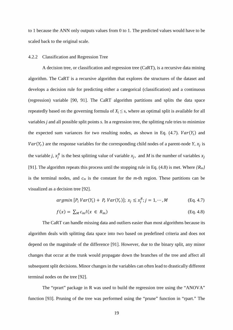
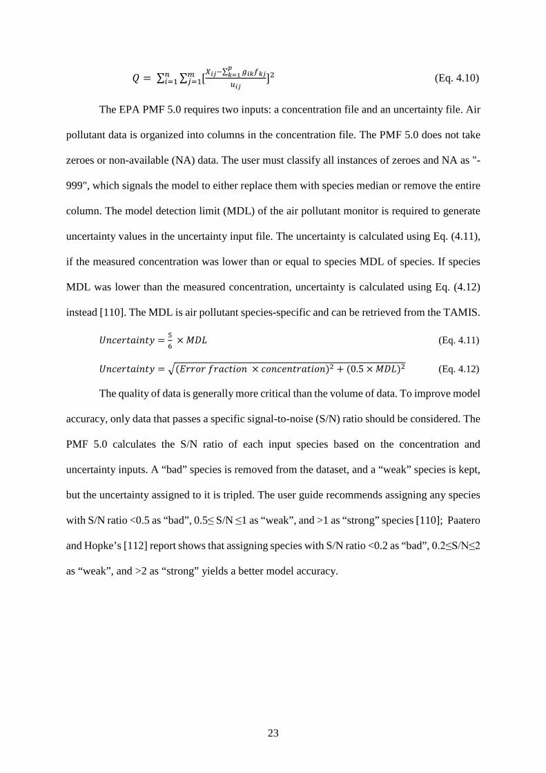
The quality of data is generally more critical than the volume of data. To improve model

accuracy, only data that passes a specific signal-to-noise (S/N) ratio should be considered. The

PMF 5.0 calculates the S/N ratio of each input species based on the concentration and

uncertainty inputs. A “bad” species is removed from the dataset, and a “weak” species is kept,

but the uncertainty assigned to it is tripled. The user guide recommends assigning any species

with S/N ratio <0.5 as “bad”, 0.5≤ S/N ≤1 as “weak”, and >1 as “strong” species [110]; Paatero

and Hopke’s [112] report shows that assigning species with S/N ratio <0.2 as “bad”, 0.2≤S/N≤2

as “weak”, and >2 as “strong” yields a better model accuracy.

24

CHAPTER 5

SPATIAL AND TEMPORAL CHARACTERISTICS OF AMBIENT ATMOSPHERIC

HYDROCARBONS IN AN ACTIVE SHALE GAS REGION IN NORTH TEXAS*

A trend analysis study was performed using the Auto-GC TNMOC concentration data

collected between 2011 and 2015 at five monitoring stations within the Barnett Shale. A 40-

minute air sample is collected by the Auto-GC monitors every hour and process through on-

board chromatography systems. However, most of the Auto-GC sites in the DFW metroplex

were built in the 2010s and did not have data points that showcased the shale gas boom and the

recession period air quality.

All five monitoring stations are within active shale gas producing counties of the

Barnett Shale; however, there were significantly lesser shale gas production activities

surrounding Flower Mound Shiloh (C1007) and Fort Worth Northwest (C13) as compared to

Eagle Mountain Lake (C75), DISH Airfield (C1013), and Decatur Thompson (C88), as shown

in Figure A9. The total natural gas production volume (MMBtu) from all producing gas wells

within each 1.2 km × 1.2 km square box between 2011 and 2015 were summed up and were

color scaled from blue (0) to red (3 × 107 MMBtu). The highest density of wells near C1007

northwest of the monitoring station and were mostly outside of the 5-km radius. At C13, there

were significantly more wells at the northwest and southeast sides, and the highest producing

wells in the area were within 5-km from the monitoring station. C75 and C1013 have

significantly higher number active wells compared to the two urban sites in all directions, and

some of the highest producing wells near the respective sites were within 5-km. Active gas

wells also surrounded C88 in all directions like the other two non-urban sites; however, the

high producing wells in the region were outside the 10-km radius.

* This chapter is reproduced from G. Q. Lim, M. Matin and K. John, "Spatial and temporal characteristics ofambient atmospheric hydrocarbons in an active shale gas region in North Texas," Science of the Total Environment, vol. 656, pp. 347-363, 2019, with permission from Elsevier.

25

Slower wind speed often leads to an increase in localized air pollution events and results

in higher ambient concentrations of air pollution near source-rich regions. On the contrary, the

effects of dispersion and rapid dilution become stronger with increasing wind speeds, which

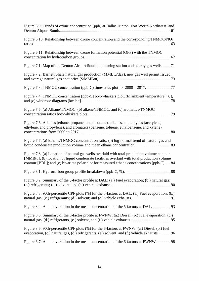
results in decreased concentration of air pollutants [113]. In Figure 5.1, the wind rose diagrams

were plotted using wind data collected from 2011 to 2015. The predominant winds at all five

monitoring stations were from the south-southeast. C1007 had the slowest recorded wind

speeds with a mean value of 8.1 kph or 2.25 m/s, whereas C75 had the fastest winds at 9.6 kph

or 2.67 m/s. The wind rose diagrams showed no significant difference between wind speed

measured at all five sites; however, C75 had a higher frequency of high-speed winds blowing

from the northwestern side of the monitoring station.

Figure 5.1: Wind rose diagrams for C1007, C13, C75, C88, and C1013: 2011-2015.

5.1 Spatial Variation in TNMOC Concentration Distribution

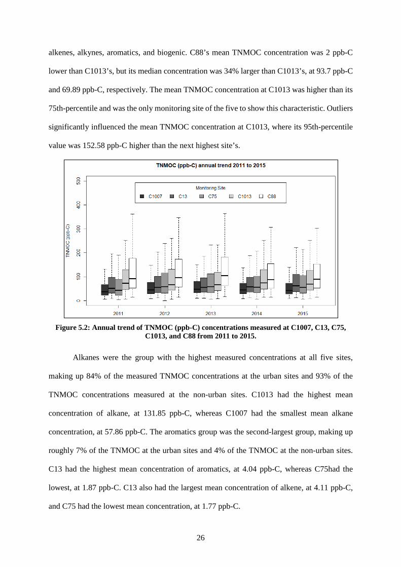
The TNMOC concentrations measured at the five sites between 2011 and 2015 are in

Figure 5.2. C1007 had the lowest TNMOC concentrations, whereas C88 had the highest. Table

5.1 highlights the summary statistics of TNMOC and the hydrocarbon groups of alkanes,

26

alkenes, alkynes, aromatics, and biogenic. C88’s mean TNMOC concentration was 2 ppb-C

lower than C1013’s, but its median concentration was 34% larger than C1013’s, at 93.7 ppb-C

and 69.89 ppb-C, respectively. The mean TNMOC concentration at C1013 was higher than its

75th-percentile and was the only monitoring site of the five to show this characteristic. Outliers

significantly influenced the mean TNMOC concentration at C1013, where its 95th-percentile

value was 152.58 ppb-C higher than the next highest site’s.

Figure 5.2: Annual trend of TNMOC (ppb-C) concentrations measured at C1007, C13, C75,

C1013, and C88 from 2011 to 2015.

Alkanes were the group with the highest measured concentrations at all five sites,

making up 84% of the measured TNMOC concentrations at the urban sites and 93% of the

TNMOC concentrations measured at the non-urban sites. C1013 had the highest mean

concentration of alkane, at 131.85 ppb-C, whereas C1007 had the smallest mean alkane

concentration, at 57.86 ppb-C. The aromatics group was the second-largest group, making up

roughly 7% of the TNMOC at the urban sites and 4% of the TNMOC at the non-urban sites.

C13 had the highest mean concentration of aromatics, at 4.04 ppb-C, whereas C75had the

lowest, at 1.87 ppb-C. C13 also had the largest mean concentration of alkene, at 4.11 ppb-C,

and C75 had the lowest mean concentration, at 1.77 ppb-C.

27

Table 5.1: Summary of TNMOC and hydrocarbon groups (ppb-C).

TNMOC Alkane Alkene Alkyne Aromatic Isoprene

C1007

Mean 65.68 57.89 2.07 0.62 3.37 2.71

Min 5.97 4.30 0.01 0.03 0.06 0.00

Median 43.45 36.31 1.61 0.51 2.45 0.55

95th 187.39 175.51 5.03 1.39 8.53 10.09

Max 3427.85 3218.73 206.70 196.53 983.97 96.37

IQR 28.3 - 73.35 21.87 - 64.87 1.06 – 2.46 0.31 – 0.78 1.56 – 4.04 0.11 – 3.2

StDev 76.61 73.11 2.65 1.16 6.79 4.83

Num. 36996 36996 36969 36531 36926 23899

C13

Mean 88.46 77.36 3.55 0.96 6.21 0.36

Min 8.82 7.04 0.18 0.02 0.25 0.01

Median 56.00 47.57 2.19 0.67 3.83 0.19

95th 271.99 242.57 11.19 2.71 19.39 1.21

Max 1791.59 1715.34 155.71 20.81 228.00 6.44

IQR 34.67 - 99.99 28.38 - 88.31 1.46 – 3.71 0.44 – 1.04 2.55 – 6.58 0.08 – 0.49

StDev 98.55 90.03 4.57 1.05 7.71 0.43

Num. 36614 36614 36614 33696 36614 27056

C75

Mean 96.55 91.44 1.71 0.56 2.66 0.59

Min 4.47 2.64 0.01 0.03 0.01 0.00

Median 54.39 50.01 1.27 0.42 1.93 0.26

95th 307.10 297.03 4.52 1.36 7.45 2.17

Max 3631.70 3499.52 29.38 12.36 118.88 20.15

IQR 30.22 - 105.17 26.98 - 99.13 0.85 – 2.01 0.25 – 0.68 1.16 – 3.29 0.09 – 0.74

StDev 140.37 137.48 1.50 0.55 2.51 0.88

Num. 36145 36145 35703 30240 35498 20727

C1013

Mean 138.22 131.92 1.84 0.54 3.67 0.46

Min 5.53 4.01 0.04 0.02 0.06 0.00

Median 69.89 64.72 1.37 0.45 2.47 0.24

95th 517.17 504.17 4.97 1.21 10.35 1.69

Max 3688.11 3649.67 42.62 14.63 195.32 9.22

IQR 44.48 - 126.74 40.58 - 118.93 0.86 – 2.21 0.28 – 0.68 1.5 – 4.25 0.09 – 0.58

StDev 223.31 219.81 1.73 0.42 4.54 0.63

Num. 36335 36335 36311 35790 36321 20313

C88

Mean 136.04 129.21 2.19 0.59 3.56 0.91

Min 14.03 10.12 0.05 0.04 0.32 0.00

Median 93.70 87.78 1.84 0.51 2.82 0.47

95th 364.59 352.37 4.56 1.26 8.10 2.36

Max 53320.20 51811.34 817.59 30.28 660.89 24.46

IQR 54.7 - 165.65 49.94 - 158 1.3 – 2.61 0.3 – 0.79 1.88 – 4.26 0.11 – 1.38

StDev 319.57 311.30 4.48 0.46 4.93 1.14

Num. 37090 37090 37088 36963 37087 20016

28

C13 and C75 had the highest and the lowest mean alkyne concentrations, respectively, where

the corresponding mean concentrations were 0.88 ppb-C and 0.47 ppb-C. The aromatic, alkene,

and alkyne TNMOC species were more prevalent in urban areas than in the non-urban areas.

The mean concentration of isoprene measured in C1007 was significantly higher than all the

other sites, at 2.71 ppb-C. The mean concentrations of isoprene at the other sites were

significantly lower than C1007’s, ranging from 0.36 ppb-C in C13 to 0.91 ppb-C in C88. The

mean isoprene concentration at C1007 was more comparable to ground-level isoprene

concentrations measured in the other major Texas cities, which ranges from 3.15 ppb-C in

Houston, Texas [114] to 6 ppb-C in Austin, Texas [115]. Isoprene is a biogenic TNMOC

species, and the most likely source was a small urban forest close to C1007.

5.2 TNMOC Components and Characteristics

Ethane, propane, and n-butane had the highest concentrations among measured

TNMOC species at all five sites, and the non-urban sites had higher concentrations of these n-

alkane species than the urban sites. These n-alkanes are common emission species from oil and

gas production activities [116, 117]. Inversely, the alkene, alkyne, and aromatic species had a

higher composition percentage at the urban sites compared to non-urban sites, and C13 had the

highest measured mean concentration of these three groups.

The ratio between each group and TNMOC was calculated to determine further the

impacts each group had on the measured TNMOC concentrations. There was a distinct

variation between the urban and non-urban sites, as shown in Figure 5.3. The urban sites’

alkane/TNMOC ratios were lower than the non-urban sites, and urban sites’ median values

were lower than the non-urban sites’ 25th percentile values. The interquartile range (IQR) for

the urban sites’ alkane/TNMOC ratio was also significantly larger than the non-urban sites’.

While the alkane/TNMOC ratios were at least 0.8 across all five sites, the alkane/TNMOC

ratios had a significant separation between the urban and the non-urban sites. C13 had a lower

29

mean concentration, lower median value, and a larger IQR, whereas C75 had a higher mean, a

higher median, and a smaller IQR.

Figure 5.3: Comparison between urban and non-urban site TNMOC concentration, alkane/TNMOC, alkene/TNMOC, alkyne/TNMOC, aromatic/TNMOC, and isoprene/TNMOC concentration ratio.

5.3 Seasonal Trend Analysis

The combination of a lower photochemical reactivity in the atmosphere coupled with

conducive meteorological conditions, such as lower mixing depths during winter months,

typically contributes to a higher measured TNMOC concentration [118, 119]. In the northern

hemisphere, the winter months are December through February, the spring months are March

30

through May, the summer months are June through August, and the fall months are September

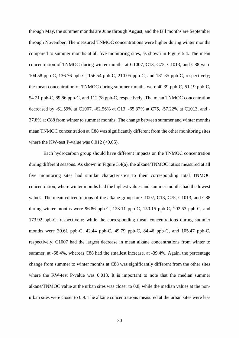
through November. The measured TNMOC concentrations were higher during winter months

compared to summer months at all five monitoring sites, as shown in Figure 5.4. The mean

concentration of TNMOC during winter months at C1007, C13, C75, C1013, and C88 were

104.58 ppb-C, 136.76 ppb-C, 156.54 ppb-C, 210.05 ppb-C, and 181.35 ppb-C, respectively;

the mean concentration of TNMOC during summer months were 40.39 ppb-C, 51.19 ppb-C,

54.21 ppb-C, 89.86 ppb-C, and 112.78 ppb-C, respectively. The mean TNMOC concentration

decreased by -61.59% at C1007, -62.56% at C13, -65.37% at C75, -57.22% at C1013, and -

37.8% at C88 from winter to summer months. The change between summer and winter months

mean TNMOC concentration at C88 was significantly different from the other monitoring sites

where the KW-test P-value was 0.012 (<0.05).

Each hydrocarbon group should have different impacts on the TNMOC concentration

during different seasons. As shown in Figure 5.4(a), the alkane/TNMOC ratios measured at all

five monitoring sites had similar characteristics to their corresponding total TNMOC

concentration, where winter months had the highest values and summer months had the lowest

values. The mean concentrations of the alkane group for C1007, C13, C75, C1013, and C88

during winter months were 96.86 ppb-C, 123.11 ppb-C, 150.15 ppb-C, 202.53 ppb-C, and

173.92 ppb-C, respectively; while the corresponding mean concentrations during summer

months were 30.61 ppb-C, 42.44 ppb-C, 49.79 ppb-C, 84.46 ppb-C, and 105.47 ppb-C,

respectively. C1007 had the largest decrease in mean alkane concentrations from winter to

summer, at -68.4%, whereas C88 had the smallest increase, at -39.4%. Again, the percentage

change from summer to winter months at C88 was significantly different from the other sites

where the KW-test P-value was 0.013. It is important to note that the median summer

alkane/TNMOC value at the urban sites was closer to 0.8, while the median values at the non-

urban sites were closer to 0.9. The alkane concentrations measured at the urban sites were less

31

consistent than the non-urban sites where a larger alkane/TNMOC IQR was measured at the

urban sites. The more abundant and more consistent alkane sources at the non-urban sites

indicated a stronger influence from oil and gas production activities.

32

33

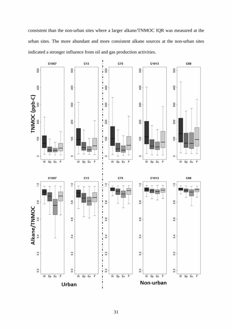
Figure 5.4: Seasonal variation of (a) TNMOC (ppb-C) and alkane/TNMOC concentration ratio, (b) alkene/TNMOC and alkyne/TNMOC concentration ratio, and (c) aromatics/TNMOC and isoprene/TNMOC concentration ratio.

Four of the five monitoring sites, minus C1013, showed alkene/TNMOC ratio

characteristics that were inverse to their respective alkane/TNMOC ratios, as shown in Figure

34

5.4(b), where the summer months had the highest ratios, followed by spring and fall, and the

winter months had the lowest ratios. At C1013, the ratios measured in spring was slightly

higher than in summer. The mean alkene concentrations measured in C1007, C13, C75, C88

and C1013 during winter months were 2.69 ppb-C, 4.69 ppb-C, 2.34 ppb-C, 2.47 ppb-C, and

2.66 ppb-C, respectively; while the mean concentrations measured during summer were 1.69

ppb-C, 2.43 ppb-C, 1.3 ppb-C, 1.42 ppb-C, and 2.03 ppb-C, respectively. The decrease in

alkene concentrations from winter to summer months ranged between -23.8% (C88) to -47%

(C13). The percentile change in-between seasons at C88 was again statistically significantly

different from the other sites with a KW-test P-value of 0.015. Despite higher alkene

concentrations during winter, the alkene/TNMOC ratios were lower during winter months

compared to the summer months. The higher summer month alkene/TNMOC ratios were the

results of lower TNMOC concentrations during summer months and a lower denominator.

There was a significantly larger decrease in the denominator (TNMOC) value from winter to

summer months compared to the numerator (alkene) value where the TNMOC concentrations

dropped by 88.17 ppb-C on average compared to the 1.19 ppb-C drop in alkene concentrations.

Common anthropogenic sources of alkynes include vehicular exhaust emissions and

industrial combustion sources. The highest alkyne/TNMOC ratios were measured during

spring at all five monitoring sites, as shown in Figure 5.4(b). At C1007, C75, C1013, and C88,

summer months had the lowest alkyne/TNMOC median values; however, at C13, the summer

month median values were higher than the fall and winter months, where winter had the lowest

median values. The mean concentration of alkyne measured during the winter months at

C1007, C13, C75, C88, and C1013 were 0.98 ppb-C, 1.23 ppb-C, 0.77 ppb-C, 0.85 ppb-C, and

0.92 ppb-C, respectively; in the summer months, the corresponding mean concentrations were

0.34 ppb-C, 0.57 ppb-C, 0.25 ppb-C, 0.28 ppb-C, and 0.3 ppb-C, respectively. C1007 had the

largest decrease in mean alkyne concentration from the winter to summer months, at 68.1%,

35

and C13 had the smallest decrease, at 53.9%. The percent-change at C13 was significantly

different from the rest of the five sites where the KW-test P-value was 0.011. The larger

alkyne/TNMOC ratios at urban sites were the result of lower TNMOC concentrations. The

most urbanized C13 had the highest measured concentration of alkyne during the summer

months and the smallest decrease in alkyne/TNMOC ratio from winter to spring, which

indicated more abundant and more consistent alkyne sources from the urban combustion

sources.

As shown in Figure 5.4(c), the median values of the aromatics/TNMOC ratios measured

at the urban sites were higher than the non-urban sites. Summer months have the highest

aromatics/TNMOC ratios, whereas the lowest ratios were during winter months, despite

aromatics concentration being the highest during winter and lowest during summer. The mean

concentration of aromatics measured during winter at C1007, C13, C75, C88, and C1013 were

4.03 ppb-C, 7.41 ppb-C, 3.26 ppb-C, 4.19 ppb-C, and 3.84 ppb-C, respectively; while their

corresponding summer mean concentrations were 2.79 ppb-C, 4.98 ppb-C, 1.98 ppb-C, 3.03

ppb-C, and 3.61 ppb-C, respectively. C75 had the highest decrease in mean aromatics

concentration between winter and summer at -39.3%, whereas C88 had the smallest drop, at

only 5.9%. The KW-test showed the difference in percentile change at C88 to be statistically

significant from all the other sites with a P-value of 0.013.

The isoprene concentrations measured at C1007 were significantly larger than the other

sites. As shown in Figure 5.4(c), the isoprene/TNMOC ratio at C1007 was considerably higher

than the other sites. The isoprene concentrations measured at all five sites were highest during

summer months and lowest during winter months. Isoprene is a biogenic emission species and

is commonly the most abundant during summer months [120]. The mean concentrations for

isoprene measured during summer months were 4.96 ppb-C for C1007, 0.63 ppb-C for C13,

0.88 ppb-C for C75, 0.67 ppb-C for C1013, and 1.38 ppb-C for C88, while their corresponding

36

mean concentrations during winter months were 0.025 ppb-C, 0.082 ppb-C, 0.013 ppb-C, 0.009

ppb-C, and 0.01 ppb-C, respectively. Summer isoprene concentrations at C1007 were 201

times larger than winter between winter concentrations; comparatively, the non-urban sites’

isoprene concentrations increased by an average of 92 times while C13 only increased by 6.7

times. The percentile increase observed at C1007 and C13 were statistically significantly

different from all other sites according to the KW-test, the P-values were 0.024 and 0.036,

respectively.

The variations in alkane concentrations were predominately responsible for the

seasonal variations in TNMOC concentrations. The change in the mean concentration of

TNMOC, alkane, alkene, and aromatics from winter to summer at C88 was statistically

significantly different from the other site. Meteorological conditions at C88 were not

significantly different from the other sites; thus, they were unlikely to have been the catalyst

behind the significant difference in the seasonal change in TNMOC, alkane, alkene, and

aromatics concentrations.

5.4 Spatio-Temporal Distribution of TNMOC

The conditional bivariate probability function (CBPF) plots for the 50th-75th percentile,

75th-95th percentile, and >95th percentile TNMOC measured at the urban and non-urban sites

are shown in Figure 5.5 and Figure 5.6, respectively. The 50th-75th percentile plot represents

average concentrations, the 75th-95th percentile plot represents high concentrations, and the

>95th percentile plot represents extreme conditions.

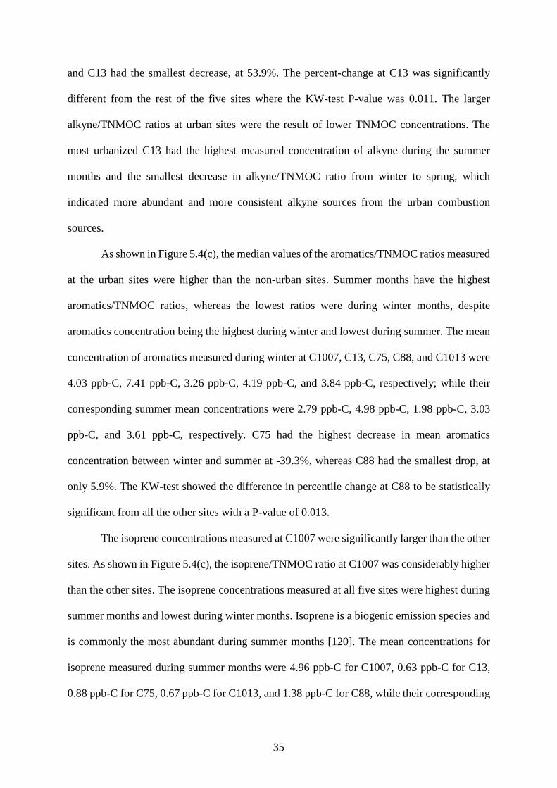
The 75th-95th percentile CBPF plot for C1007 and C13 had high concentration regions

that match the gas well surrounding the sites. The majority of the gas wells surrounding C1007

are on the west-northwest-north sides of the monitoring station, which coincides with the 75th-

95th TNMOC CBPF. The 50th-75th CBPF at C13 showed similarities to the gas wells producing

less than 1 × 107 MMBtu (blue squares) on Figure A9, whereas the 75th-95th CBPF plot

37

resembles the pattern formed by the gas wells producing between 1 × 107 and 2 × 107 MMBtu

(green squares). C75’s 50th-75th TNMOC CBPF also resembles the gas wells surrounding the

monitoring station. The other two CBPF plots from C75 showed the highest probability at the

northwest side of the monitoring station, which did not visually match the gas-producing wells

at the site. Gas wells at C88 had the highest productivity at the southeast and the northwest end

of the map, while the 75th-95th CBPF at C1013 had some similarities to its gas production map,

as seen in the highest density of wells in the west-northwest-north side of the monitoring

station.

Figure 5.5: Conditional Bivariate Probability Function plot for 50th to 75th percentile, 75th to 95th percentile, and >95th percentile at C1007 and C13.

38

Figure 5.6: Conditional Bivariate Probability Function plot for 50th to 75th percentile, 75th to 95th percentile, and >95th percentile at C75, C1013, and C88.

39

The CBPF plot shows two higher probability regions, one in the gas well-dense region

northwest of the C1013 site and one just south of it. The 50th-75th CBPF also showed a high

concentration region at the southeast end of the plot. The Atmos Energy facility is located just

south of the monitoring station and was likely the source of this emission. The 75th-95th and the

over-95th CBPF plots showed similarities to the gas wells where the highest probability regions

were either dense with gas wells (75th-95th plot) or having high production volume (95th plot).

The 50th-75th CPBF at C88 had the highest probability at the southeast end of the plot, which

was likely emissions from the densely packed gas wells at the southeast end. High probability

regions on the >95th CBPFs were on the west side of C1007 and C13, northwest side of C75

and C1013, and both northwest and southeast sides of C88.

5.5 Summary Findings

The emissions from unconventional oil and gas production activities within the Barnett

Shale region has had a significant impact on the measured TNMOC concentrations at five

ambient air quality monitoring stations in North Texas during 2011-2015. TNMOC

concentrations observed at the non-urban sites were, on average, 1.61 times larger than those

at urban sites. Alkanes, predominately ethane, were among the most significant contributors to

the overall measured TNMOC concentrations. Approximately 88% of the measured TNMOC

concentrations at urban sites and 95% of the TNMOC at non-urban sites were n-alkanes.

Despite the higher measured concentrations of n-alkanes, the urban sites also were influenced

by anthropogenic sources of VOC from motor vehicles and industries, as highlighted by higher

alkene, alkyne, and aromatics/TNMOC ratios. The IQR in alkane/TNMOC ratios at the urban

sites were also larger than at non-urban sites. While all sites were close to nearby oil and gas

activities, there was an evident spatio-temporal variation in the measured TNMOC

concentration between the urban and non-urban sites. The measured TNMOC concentrations

experienced winter highs and summer lows. However, one of the non-urban sites (C88) was

40

impacted by VOC year-round from nearby oil and gas production activities. Also, there were

significantly elevated isoprene concentrations from biogenic emissions at C1007. The impact

of elevated concentrations of TNMOC from oil and gas sources will be an essential factor in

understanding the nature of local and regional air quality in North Texas.

41

CHAPTER 6

A LONG-TERM TREND ANALYSIS OF AIR QUALITY IN THE DALLAS-FORT

WORTH AREA: DISCERNING THE IMPACT OF OIL AND GAS EMISSIONS FROM

THE BARNETT SHALE

With the increase in exploration for and extraction of unconventional energy sources

on a global scale, the impact of unconventional shale gas emissions on air quality has become

an increasingly important factor. In this chapter, a long-term study on ground-level ozone and

its precursors was conduction using concentration data collected from 2000 to 2018. Air

pollutant concentration data from monitoring stations at locations with the following

characteristics were retrieved: (i) highly urbanized region with no oil and gas operations (Dallas

Hinton, DAL), (ii) moderately urbanized region with significant oil and gas operations (Fort

Worth Northwest, FWNW), and (iii) exurban region with a large amount of oil and gas

operations (Denton Airport South, DEN). The air pollutant concentration data is on the TAMIS.

Ozone, NOx, CO, and TNMOC concentrations collected between January 1, 2000, and

December 31, 2018, were used. Ozone and NOx concentrations were available in hourly

updated values at all three sites. Hourly CO concentration was only available at DAL and

FWNW; however, FWNW discontinued its CO monitoring in 2014. While hourly updated

TNMOC samples were available in DAL and FWNN, DEN only had access to daily averaged

values. These daily averaged TNMOC values were updated every sixth-day. They are collected

using steel SUMMA canisters and are analyzed using gas chromatograph-mass spectrometers

by TCEQ scientists [33]. Also, FWNW had only started collecting TNMOC samples in

November 2003. Since the sixth-day cannister TNMOC data were available for all three sites,

we had decided to use this dataset in the study.

Table 6.1 shows the 2008, 2011 and 2014 National Emissions Inventory (NEI) for

Criteria and Hazardous Air Pollutants by 60 Emissions Inventory System (EIS) emission

42

sectors of CO, NOx, and volatile organic compound (VOC) for Dallas, Tarrant, and Denton

county [121]. VOC is synonymous with TNMOC, except for the inclusion of methane

concentrations. The U.S. EPA maintains and updates the NEI database every three years.

However, the EIS data before 2008 was not publicly available, and the 2017 data was not ready

at the time of writing this paper. Dallas county had the highest emissions for all three pollutant

types, followed by Tarrant and Denton counties. Also, the emission trends of all three pollutant

types were in the decrease between 2008 and 2014.

Table 6.1: National Emissions Inventory (NEI) for Criteria and Hazardous Air Pollutants by 60 Emissions Inventory System (EIS) emission sectors of VOC, CO, and NOx (tons) [121].

2008 2011 2014 Change (%/Year)

Dallas

NOx 62,707.54 51,422.35 45,223.37 -4.65%

CO 309,104.00 287,281.23 249,323.80 -3.22%

VOC 68,678.98 56,808.05 50,763.77 -4.35%

Tarrant

NOx 65,053.60 45,081.84 34,374.22 -7.86%

CO 203,221.49 200,727.20 151,909.60 -4.21%

VOC 55,176.21 50,651.33 45,873.04 -2.81%

Denton

NOx 20,877.80 13,784.60 12,331.40 -6.82%

CO 62,935.37 60,568.24 50,934.00 -3.18%

VOC 29,722.38 27,267.55 25,050.71 -2.62%

Temperature, relative humidity, and wind speed play essential roles in ozone production

and destruction [122, 123]. Between 2000 and 2018, the regional outdoor temperature

increased while relative humidity decreased. The fastest winds (Figure A1) occurred during

spring, and the mean wind speed at DAL, FWNW, and DEN were 8.87 km/hour, 11.92

km/hour, and 11.51 km/hour, respectively. Aside from slightly slower wind speeds at DAL, all

three sites had very similar meteorological conditions. Thus, the variation in air pollutant

concentrations was unlikely to be caused by meteorological conditions. Figure A1 shows the

seasonal wind rose diagram of each monitoring station. Throughout the year, the winds are

43

predominantly southeasterly. Since the monitoring stations were on the eastern end of the

Barnett Shale, fugitive emissions from the Barnett Shale had to be carried in by westerly winds,

which are uncommon in the region. Hence, any traces of oil and gas emissions found at the

monitoring stations are mainly from local sources.

The study period was divided into four distinct periods: 2000-2006, 2007-2009, 2010-

2012, and 2013-2018. Between December 2007 and June 2009, the U.S. economy went through

a period of turmoil. It ultimately resulted in an economic recession, and this also influenced

energy demand and production, which also had a downturn [124]. The observations made

between 2000 and 2006 represented the pre-recession period, where the Barnett Shale region

saw a massive expansion in shale gas operations. The 2010-2012 period saw the rebound of

the U.S. economy and energy production demand. Finally, the 2013-2018 period saw a drop in

natural gas productions across the Barnett Shale post-2013 due to low natural gas prices [2].

6.1 Oxides of Nitrogen (NOx)

Conventional urban anthropogenic sources of NOx, a precursor to the ozone formation,

include gasoline vehicle exhaust, commercial and industrial solvent uses, and power plant

emissions [43, 44]. Heavy-duty off-road trucks are used to bring materials to and from the gas

wells, and these trucks emit NOx [125]. There are not many stationary NOx emission sources,

outside of diesel-powered trucks, on shale gas production sites. Thus, NOx is a good indicator

of conventional urban sources.

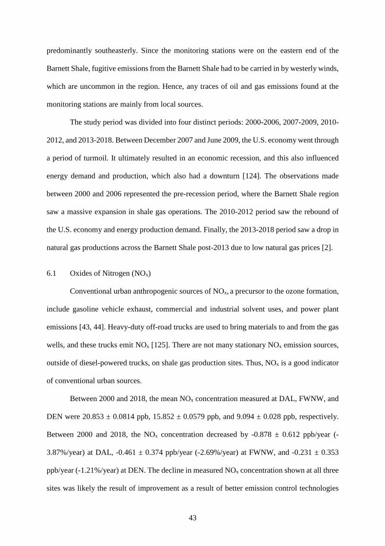
Between 2000 and 2018, the mean NOx concentration measured at DAL, FWNW, and

DEN were 20.853 ± 0.0814 ppb, 15.852 ± 0.0579 ppb, and 9.094 ± 0.028 ppb, respectively.

Between 2000 and 2018, the NOx concentration decreased by -0.878 ± 0.612 ppb/year (-

3.87%/year) at DAL, -0.461 ± 0.374 ppb/year (-2.69%/year) at FWNW, and -0.231 ± 0.353

ppb/year (-1.21%/year) at DEN. The decline in measured NOx concentration shown at all three

sites was likely the result of improvement as a result of better emission control technologies

44

and the effective implementation of emissions regulation policies [126, 127]. While the mean

and 90th-percentile NOx concentrations at DAL and FWNW had decreased consistently since

2000, DEN’s concentration saw an increase from 2002 to 2005, and then followed by a decline

post-2006, as shown in Figure 6.1. We suspect the increase in measured NOx concentrations at

DEN from 2002 to 2005 was likely caused by high truck traffic during the development phase

as the NOx emissions from diesel-powered vehicles are significantly higher than gasoline-

powered vehicles [128].

Figure 6.1: Trends of NOx concentration (ppb) at Dallas Hinton, Fort Worth Northwest, and Denton Airport South.

The mean concentration of NOx measured at DAL during 2000-2006, 2007-2009, 2010-

2012, and 2013-2018 were 29.2 ± 0.177 ppb, 20.7 ± 0.201 ppb, 17.5 ± 0.151 ppb, and 13.7 ±

0.09 ppb, respectively. The mean concentration of NOx at DAL had decreased by -0.53 ± 1.64

ppb/year (-1.23%/year) during 2000-2006, -3.55 ± 0.05 ppb/year (-15.86%/year) during 2007-

2009, -0.95 ± 0.95 ppb/year (-5.25%/year) during 2010-2012, and -0.94 ± 0.72 ppb/year (-

5.63%/year) during 2013-2018. The mean NOx concentration measured at FWNW during

2000-2006, 2007-2009, 2010-2012, and 2013-2018 were 19.8 ± 0.114 ppb, 18.4 ± 0.151 ppb,

45

13.9 ± 0.132 ppb, and 11.1 ± 0.073 ppb, respectively. Despite an overall downward trend, the

annual mean NOx concentration saw a slight increase from 2000 to 2006 and from 2010 to

2012, at the rate of +0.083 ± 0.592 ppb/year (+0.66%/year) and +0.1 ± 1.4 ppb/year

(+1.22%/year), respectively. The mean concentration of NOx saw a decline by -3.05 ± 0.05

ppb/year (-15.36%/year) during 2007-2009 during the recession and -0.4 ± 0.5 ppb/year (-

2.98%/year) during 2013-2018. The mean concentration of NOx measured at DEN was 11 ±

0.053 ppb during 2000-2006, 9.44 ± 0.069 ppb during 2007-2009, 8.01 ± 0.067 ppb during

2010-2012, and 7.24 ± 0.038 ppb during 2013-2018. The mean NOx concentration increased

by +0.03 ± 0.91 ppb/year (+1.51%/year) during 200-2006, followed by decreased

concentrations during the next three periods. The mean NOx concentration decreased at the rate

of -1.625 ± 0.215 ppb/year (-16%/year), -0.425 ± 0.275 ppb/year (-5.17%/year), and -0.286 ±

0.529 ppb/year (-2.2%/year) during 2007-2009, 2010-2012, and 2013-2018, respectively.

The NEI for NOx (Table 6.1) had decreased by -4.65%/year at DAL, -7.86%/year at

FWNW, and -6.82%/year at DEN between 2008 and 2014. During the same period, the mean

concentration of NOx measured at DAL, FWNW, and DEN had decreased by -5.05%/year, -

7.12%/year, and -2.5%/year, respectively. The decreased in the measured concentrations at

DAL and FWNW were very within a ±1% different from the decrease in the NEI for their

respective counties. Both the measured concentrations at DEN and the NEI for Denton county

experienced a decline between 2008 and 2014. However, the percent change in NEI was more

significant than the percent change in the measured concentration of NOx at DEN. Thus, it

appears that the percent reduction in NEI for NOx in Denton county may not accurately reflect

the local NOx emissions from sources surrounding DEN.

6.2 Carbon Monoxide (CO)

Carbon monoxide (CO) is a combustion by-product closely associated with traffic and

power plant emissions. Conventional urban anthropogenic emission sources can also be

46

quantified using measured CO concentrations. A high CO concentration is an indicator of

fossil-based fuel combustion sources, including gasoline vehicle exhaust and power plant

emissions. CO can react with hydroxyl radicals (OH) to form hydroperoxyl radical (HO2) and

carbon dioxide (CO2), which can lead to ground-level ozone formation [129].

Figure 6.2: Trends of CO concentration (ppm) at Dallas Hinton and Fort Worth Northwest.

The mean concentration of CO measured at DAL between 2000 and 2018 was 0.299 ±

0.0006 ppm, whereas the mean concentration of CO measured at FWNW from 2000 to 2014

was 0.322 ± 0.0006 ppm. DAL and FWNW both saw a decrease in the mean and 90th-percentile

CO concentrations, as shown in Figure 6.2. At the beginning of the monitoring period in 2000,

the mean and 90th-percentile CO concentrations at FWNW was larger than DAL. While both

sites saw an increase in CO concentration between 2002 and 2003, the increase at DAL was

more significant than FWNW from 2003 through 2011 as a result of a higher mean and 90th-

percentile CO concentrations at DAL. In 2012, the CO concentration at FWNW was higher

than DAL. It remained above that recorded in DAL until the monitoring stopped in 2015.

Between 2000 and 2018, the mean concentration of CO at DAL decreased by -0.009 ± 0.009

47

ppm/year (-2.38%/year), whereas FWNW saw a decrease at the rate of -0.023 ± 0.01 ppm/year

(-5.85%/year) between 2000 and 2014.

The mean concentration of CO at DAL had experienced a decrease across all four

periods. The mean concentrations of CO measured during 2000-2006, 2007-2009, 2010-2012,

and 13-08 were 0.384 ± 0.0012 ppm, 0.328 ± 0.0015 ppm, 0.255 ± 0.0009 ppm, and 0.214 ±

0.0006 ppm, respectively. The mean concentration of CO decreased by -0.0085 ± 0.022

ppm/year (-1.46%/year), -0.0405 ± 0.0185 ppm/year (-11.48%/year), -0.0275 ± 0.0565

ppm/year (-8.84%/year), and -0.0034 ± 0.0096 ppm/year (-1.09%/year) during 2000-2006,

2007-2009, 2010-2012, and 13-08, respectively.

At FWNW, the mean concentration of CO was 0.405 ± 0.0011 ppm during 2000-2006,

0.266 ± 0.001 ppm during 2007-2009, and 0.238 ± 0.0009 ppm during 2010-2012. During

2000-2006 and 2007-2009, the mean concentration of CO had decreased by -0.035 ± 0.022

ppm/year (-7.17%/year) and -0.0255 ± 0.0215 ppm/year (-8.62%/year), respectively. Despite

a lower mean concentration during 2010-2012 than the previous period, the mean concentration

of CO during 2010-2012 increased by +0.016 ± 0.019 ppm/year (+7.12%/year). The increased

in CO concentrations observed during 2010-2012 was also observed in the NOx concentrations

measured during the 2010-2012 period.

Between 2008 and 2014, the CO emissions in Dallas and Tarrant counties (Table 6.1)

had decreased by -3.22%/year and -4.21%/year, respectively. During the same timeframe, the

mean concentration of measured CO from DAL and FWNW had experienced a decrease at the

rate of -5.4%/year and -2.31%/year, respectively. While the NEI and measured concentrations

both showed decreases, the percent change in the measured concentrations of CO at DAL was

significantly higher than the NEI for Dallas county whereas the percent change in the measured

concentrations at FWNW was lower than the decreased in Tarrant county NEI for CO. The

NEI for CO were countywide estimations whereas the measured concentrations are the result

48

of local emission sources and the percent change in CO emissions are not necessarily uniform

across the county.

Incomplete combustion of gasoline is the primary source of CO in an urban region. The

decreased in measured CO concentration at DAL and FWNW was likely achieved through the

improvements in vehicle engine efficiency and exhaust control technologies [126, 127].

6.3 Total Non-Methane Organic Carbon (TNMOC)

TNMOC are carbon compounds that react photochemically in the atmosphere.

TNMOC includes compounds with low photochemical reactivity, such as methane and ethane,

but excludes carbon monoxide (CO), CO2, carbonic acid, and carbonates. In a typical urban

region, TNMOC sources include vehicular exhaust emissions, fossil fuel combustion, power

plant emissions, industrial and domestic solvent use, oil and gas production facilities, and

fugitive emission leaking from pipelines and storage tanks of fuels.

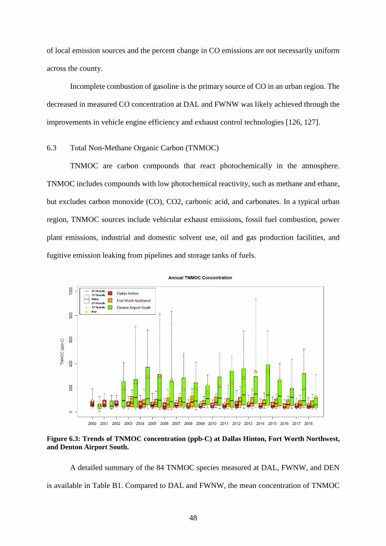
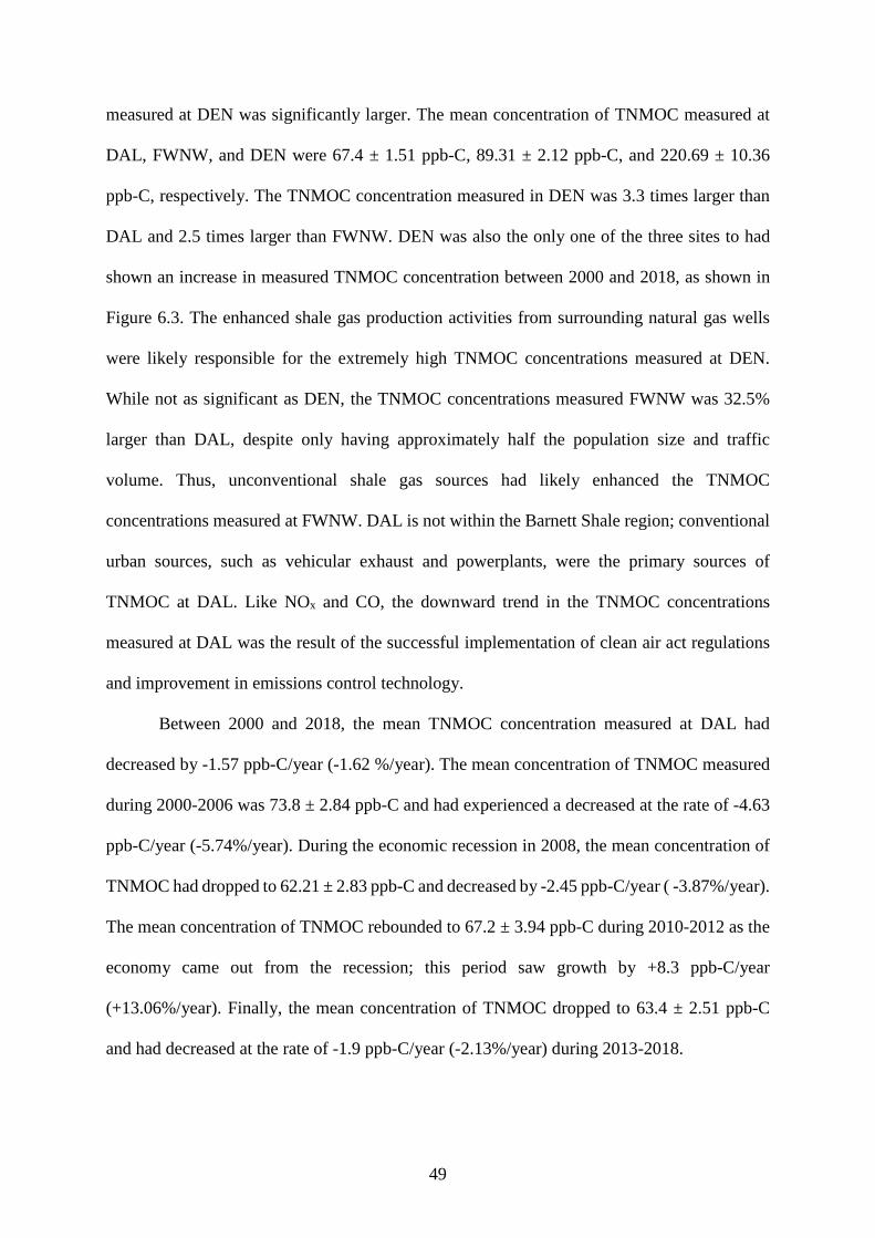
Figure 6.3: Trends of TNMOC concentration (ppb-C) at Dallas Hinton, Fort Worth Northwest, and Denton Airport South.

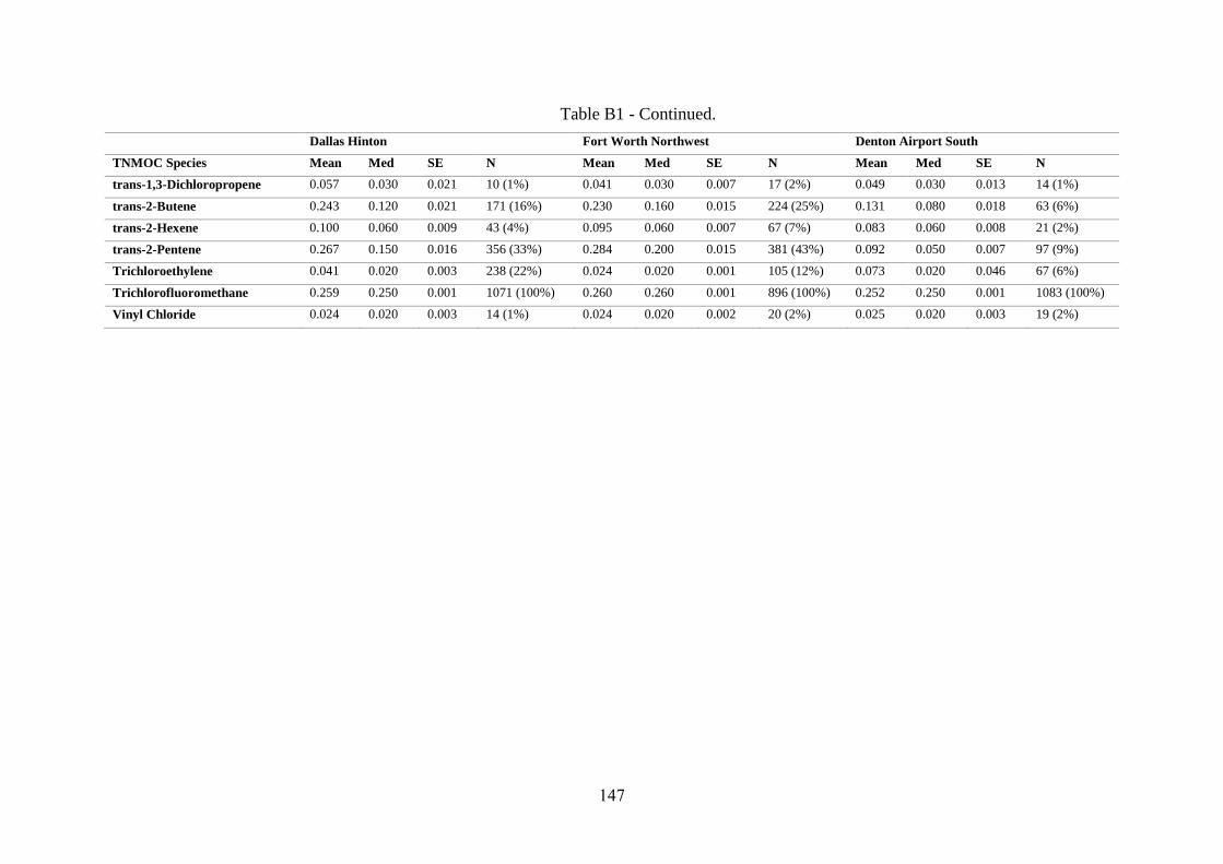
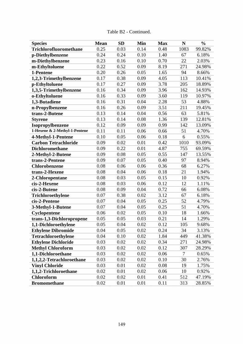
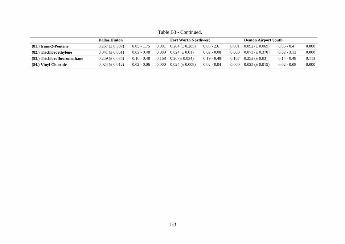
A detailed summary of the 84 TNMOC species measured at DAL, FWNW, and DEN

is available in Table B1. Compared to DAL and FWNW, the mean concentration of TNMOC

49

measured at DEN was significantly larger. The mean concentration of TNMOC measured at

DAL, FWNW, and DEN were 67.4 ± 1.51 ppb-C, 89.31 ± 2.12 ppb-C, and 220.69 ± 10.36

ppb-C, respectively. The TNMOC concentration measured in DEN was 3.3 times larger than

DAL and 2.5 times larger than FWNW. DEN was also the only one of the three sites to had

shown an increase in measured TNMOC concentration between 2000 and 2018, as shown in

Figure 6.3. The enhanced shale gas production activities from surrounding natural gas wells

were likely responsible for the extremely high TNMOC concentrations measured at DEN.

While not as significant as DEN, the TNMOC concentrations measured FWNW was 32.5%

larger than DAL, despite only having approximately half the population size and traffic

volume. Thus, unconventional shale gas sources had likely enhanced the TNMOC

concentrations measured at FWNW. DAL is not within the Barnett Shale region; conventional

urban sources, such as vehicular exhaust and powerplants, were the primary sources of

TNMOC at DAL. Like NOx and CO, the downward trend in the TNMOC concentrations

measured at DAL was the result of the successful implementation of clean air act regulations

and improvement in emissions control technology.

Between 2000 and 2018, the mean TNMOC concentration measured at DAL had

decreased by -1.57 ppb-C/year (-1.62 %/year). The mean concentration of TNMOC measured

during 2000-2006 was 73.8 ± 2.84 ppb-C and had experienced a decreased at the rate of -4.63

ppb-C/year (-5.74%/year). During the economic recession in 2008, the mean concentration of

TNMOC had dropped to 62.21 ± 2.83 ppb-C and decreased by -2.45 ppb-C/year ( -3.87%/year).

The mean concentration of TNMOC rebounded to 67.2 ± 3.94 ppb-C during 2010-2012 as the

economy came out from the recession; this period saw growth by +8.3 ppb-C/year

(+13.06%/year). Finally, the mean concentration of TNMOC dropped to 63.4 ± 2.51 ppb-C

and had decreased at the rate of -1.9 ppb-C/year (-2.13%/year) during 2013-2018.

50

From 2004 to 2018, the mean concentration of TNMOC measured at FWNW saw a

slight decrease of -0.81 ppb-C/year (-0.63%/year). The mean concentration of TNMOC during

2000-2006 was 88.2 ± 5.11 ppb-C, and it increased slightly by +0.75 ppb-C/year

(+0.91%/year). While the mean concentration of 93.4 ± 4.24 ppb-C was higher when compared

to the preceding period, TNMOC concentrations had experienced a decreased by -6.1 ppb-

C/year (-6.19%/year) during 2007-2009. The mean concentration of TNMOC measured during

2007-2009 was 101.5 ± 5.6 ppb-C and saw an increase of +2.5 ppb-C/year (+2.51%/year).

Lastly, the mean concentrations dropped to 81.4 ± 2.96 ppb-C had decreased by -4ppb-C/year

(-4.43%/year) during 2013-2018.

DEN was also the only site to had shown an increase in the mean concentrations of

TNMOC between 2000 and 2018 at the rate of +3.59 ppb-C/year (+9.97%/year). The mean

concentrations of TNMOC measured at DEN during 2000-2006 was 211 ± 17.6 ppb-C, and

there was a +34.61 ppb-C/year (+37.53%/year) increase in the mean concentrations measured

during this period. During the recession period of 2007-2009, the mean concentrations dropped

to 178.3 ± 16.3 ppb-C, which corresponds to a decreased by -11 ppb-C/year (-5.88%/year).

During 2010-2012, the mean concentration of TNMOC was 243.7 ± 23.3 ppb-C and saw an

increased by +34.5 ppb-C/year (+15.14%/year). The mean concentration of TNMOC dropped

to 241 ± 25 ppb-C and saw a decline by -42.4ppb-C/year (-16.69%/year) during 2013-2018.

Between 2008 and 2014, the NEI for VOC (Table 6.1) decreased by -4.35%/year in

Dallas county, -2.81%/year in Tarrant county, and -2.62%/year in Denton county. During 2008-

2014, the measured TNMOC concentrations at FWNW had a similar percent change as the

NEI for Tarrant county, at the rate of -2.42%/year. However, DAL and DEN both saw an

increase in the mean concentration of the TNMOC measured in the same period, at the rate of

+0.48%/year and +13.37%/year, respectively. At DAL, the mean concentrations of TNMOC

saw an increase during the 2010-2012 period as the economy was recovering from the 2008

51

recession. The NEI shows that the VOC emissions in Dallas county were decreasing during

2008-2014. However, the decline may not be reflected in the emissions surrounding downtown

Dallas, which is one of the largest economic hubs in the state of Texas. Despite a decreased in

the NEI for VOC in Denton county, the measured TNMOC concentrations at DEN had

increased significantly during 2008-2014. Extremely localized emission sources may impact

the TNMOC concentrations measured at DEN. Also, the percent change in the NEI for VOC

may not have accurately reflected the percent change in slow reactive hydrocarbon species.

These slow reactive species more commonly found in unconventional emission sources, which

include shale gas production.

6.3.1 Benzene, Toluene, Ethylbenzene, and Xylene (BTEX)

Benzene, toluene, ethylbenzene, and xylene (BTEX) falls under the U.S. EPA’s

hazardous air pollutants (HAPs) list, which contains 189 pollutants [130]. Exposure to elevated

concentrations of BTEX can lead to eye, nose, and throat irritation, asthma, and increased risk

of cancer [131].

DAL had the highest mean concentration of BTEX (sum of mean concentrations of

each species) at 7.529 ± 0.825 ppb-C, followed by FWNW at 6.303 ± 0.83 ppb-C, and finally

DEN at 5.384 ± 1.099 ppb-C. There was a significant outlier in the measured concentrations at

DEN. The mean concentration of toluene measured in 2004 at DEN (8.83 ppb-C) was

significantly higher than the rest of the monitoring period (mean of 2.45 ppb-C). Removing the

outlier, the mean concentration of BTEX was shown to be in decline at all three sites between

2000 to 2018 at the rate of -0.263 ppb-C/year (-2.08%/year) in DAL, -0.183 ppb-C/year (-

2.19%/year) in FWNW, and -0.141 ppb-C/year (-1.99%/year) in DEN. Figure 6.4 shows the

annual median concentration of each BTEX species at the three sites. The median

concentrations in 2018 were significantly lower than the beginning of the monitoring period at

all three sites.

52

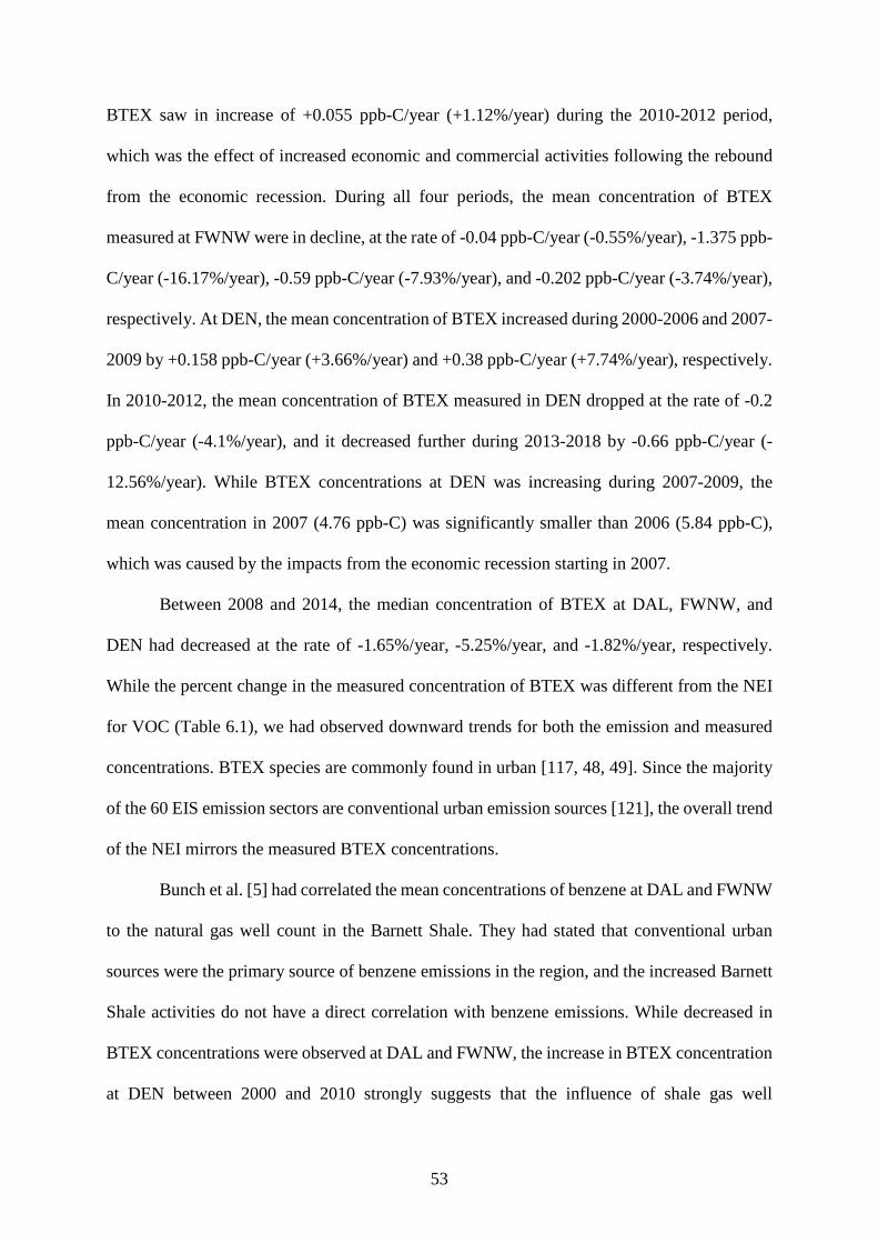
Figure 6.4: Trend of median BTEX concentrations (ppb-C) in Dallas Hinton, Fort Worth Northwest, and Denton Airport South.

The mean concentration of BTEX measured at DAL had decreased during 2000-2006,

2007-2009, and 2013-2018 at the rate of -0.677 ppb-C/year (-6.82%/year), 0.71 ppb-C/year (-

9.92%/year), and -0.164 (-0.92%/year), respectively. However, DAL’s mean concentration of

53

BTEX saw in increase of +0.055 ppb-C/year (+1.12%/year) during the 2010-2012 period,

which was the effect of increased economic and commercial activities following the rebound

from the economic recession. During all four periods, the mean concentration of BTEX

measured at FWNW were in decline, at the rate of -0.04 ppb-C/year (-0.55%/year), -1.375 ppb-

C/year (-16.17%/year), -0.59 ppb-C/year (-7.93%/year), and -0.202 ppb-C/year (-3.74%/year),

respectively. At DEN, the mean concentration of BTEX increased during 2000-2006 and 2007-

2009 by +0.158 ppb-C/year (+3.66%/year) and +0.38 ppb-C/year (+7.74%/year), respectively.

In 2010-2012, the mean concentration of BTEX measured in DEN dropped at the rate of -0.2

ppb-C/year (-4.1%/year), and it decreased further during 2013-2018 by -0.66 ppb-C/year (-

12.56%/year). While BTEX concentrations at DEN was increasing during 2007-2009, the

mean concentration in 2007 (4.76 ppb-C) was significantly smaller than 2006 (5.84 ppb-C),

which was caused by the impacts from the economic recession starting in 2007.

Between 2008 and 2014, the median concentration of BTEX at DAL, FWNW, and

DEN had decreased at the rate of -1.65%/year, -5.25%/year, and -1.82%/year, respectively.

While the percent change in the measured concentration of BTEX was different from the NEI

for VOC (Table 6.1), we had observed downward trends for both the emission and measured

concentrations. BTEX species are commonly found in urban [117, 48, 49]. Since the majority

of the 60 EIS emission sectors are conventional urban emission sources [121], the overall trend

of the NEI mirrors the measured BTEX concentrations.

Bunch et al. [5] had correlated the mean concentrations of benzene at DAL and FWNW

to the natural gas well count in the Barnett Shale. They had stated that conventional urban

sources were the primary source of benzene emissions in the region, and the increased Barnett

Shale activities do not have a direct correlation with benzene emissions. While decreased in

BTEX concentrations were observed at DAL and FWNW, the increase in BTEX concentration

at DEN between 2000 and 2010 strongly suggests that the influence of shale gas well

54

developments. Increased truck traffic in the region during the development phases of wells

likely had caused the increase in BTEX concentration at DEN.

6.3.2 Natural Gas Production Impacts on TNMOC Levels

Tarrant and Denton are two major shale gas producing counties within the Barnett

Shale. Since DAL is outside of the shale gas region, and there were no gas wells built within

5-km of the monitoring station. Figure 6.5 shows the number of active gas wells within 5-km

from FWNW and DEN; and their total annual production. By the end of 2018, there were 157

active gas wells within 5-km of FWNW and 213 active gas wells within 5-km of DEN. From

2000 to 2018, the gas wells within 5-km from FWNW and DEN produced a total of 2.75 × 108

MMBtu and 2.5 × 108 MMBtu in natural gas, respectively. Between 2003 and 2012, FWNW

saw an increased in the number of active gas wells surrounding the monitoring station, which

correlated well with the increase in measured TNMOC concentrations during this period.

Figure 6.5: Number of active gas wells within 5-km from Fort Worth Northwest and Denton Airport South along with the total natural gas production volume (MMBtu).

The emissions released during the development and production phases of these gas wells

contributed significantly to the growth in TNMOC concentrations at FWNW through 2011

55

(Figure 6.3). While the number of active gas wells surrounding FWNW had stayed relatively

constant since 2012, their production volume had dropped significantly. There was a decline

in natural gas production across the Barnett Shale gas region due to a drop in natural gas prices

[2]. The TNMOC concentrations post-2012 also showed a similar trend to the natural gas

production volume from the gas wells that surround FWNW.

The 90th-percentile value of TNMOC measured at DEN had two peaks, one in 2006

and the other in 2013 (Figure 6.3); both peaks were followed by a decrease, as shown during

2007-2009 and 2013-2018. There was a substantial increase in the number of active wells

surrounding DEN from 2000 through 2006. The increased gas well development activities had

contributed to a rapid increase in the measured TNMOC concentrations, peaking in 2006.

Starting in 2007, the growth in the number of active gas wells had significantly dropped due to

the economic depression; this had contributed to the decrease in TNMOC concentrations

during the 2007-2009 period. The production volume from the gas wells surrounding DEN

increased consistently from 2009 through 2014, and this culminated in a peak in mean

concentrations of TNMOC during 2013-2014. Since 2014, natural gas production volumes

have dropped significantly. As a result, there was a substantial decrease in the measured

TNMOC concentrations during 2013-2018.

Acetylene/TNMOC and ethane/TNMOC concentration ratios were used to identify the

changes in emissions from vehicle exhaust and natural gas sources, respectively. Ethane is a

TNMOC species found abundantly in oil and gas emissions, whereas high concentrations

acetylene points to fossil fuel burning and vehicular exhaust emissions [48, 49, 50, 51, 117,

132]. The mean of acetylene/TNMOC concentration ratios calculated for DAL, FWNW, and

DEN was 0.028 ± 0.0007, 0.019 ± 0.0004, and 0.01 ± 0.0004, respectively; whereas the mean

of ethane/TNMOC concentration ratios was 0.229 ± 0.002 at DAL, 0.296 ± 0.003 at FWNW,

and 0.342 ± 0.003 at DEN. Figure 6.6 shows all a decrease in the acetylene/TNMOC

56

concentration ratio and an increase in the ethane/TNMOC concentration ratio at all three sites.

Figure 6.6: Trends of acetylene/TNMOC, ethane/TNMOC, CO/TNMOC, and NOx/TNMOC concentration ratio.

Like acetylene, CO, and NOx concentrations in urban regions are also usually emitted from

vehicular exhaust sources. The mean of CO/TNMOC concentration ratios was 5.467 ± 0.105

at DAL and 4.184 ± 0.117 at FWNW. In contrast, the mean of NOx/TNMOC concentration

ratios was 0.298 ± 0.004, 0.176 ± 0.003, and 0.0995 ± 0.003 at DAL, FWNW, and DEN,

respectively. CO/TNMOC and NOx/TNMOC concentration ratios increased during 2000-2004

57

but was followed by a continued decrease throughout 2018 except for a slight increase during

2010-2011. The acetylene/TNMOC, CO/TNMOC, and NOx/TNMOC concentration ratios all

followed a similar downward trend. The decline indicates deceased impacts from the gasoline-

powered vehicular exhaust and other combustion-related sources. On the other hand, the

increase in ethane/TNMOC concentration ratios suggests the increased impacts of

unconventional oil and gas emissions in the region.

According to Baker et al. [133], the typical concentrations of propane in U.S. cities

during summertime is between the range of 0.87 ppb-C to 10.53 ppb-C. The mean

concentrations of propane measured during summertime at DAL and FWNW were 6.283 ±

0.167 ppb-C and 8.02 ± 0.307 ppb-C, respectively, and were both within the range observed in

other major U.S. cities. The mean concentration of propane measured in DEN during

summertime was 26.028 ± 2.62 ppb-C, which was much higher than the typical urban propane

concentrations. The mean concentration of summertime propane measured at DEN more

closely resembled the concentrations measured at other oil and gas regions. The concentration

fall between the concentrations measured at Colorado’s Northern Front Range metropolitan

area (24 ppb-C) [134] and the Marcellus Shale (39 ppb-C) [135].

Figure 6.7: Relationship between isopentane and n-pentane at Dallas Hinton, Fort Worth Northwest, and Denton Airport South.

Oil and gas production-related emissions can be differentiated from gasoline-powered

58

vehicular emissions through isopentane/n-pentane concentration ratios. Regions with higher

vehicle emissions have isopentane/n-pentane ratios greater than one. In contrast, regions with

higher natural gas emissions have an isopentane/n-pentane ratio under one and closer to 0.9

[135]. As shown in Figure 6.7, DAL and FWNW have isopentane/n-pentane ratios higher than

one, at 1.931 and 1.514, respectively. DEN’s ratio was lower than one, at 0.959. Thus, there

was a stronger impact from gasoline vehicle sources at DAL and FWNW, while DEN had a

stronger impact from natural gas sources.

While the gas wells surrounding FWNW had the highest total production volume

among the three, FWNW showed a weaker influence from the oil and gas activities compared

to DEN. We suspected that local legislatures and regulations on gas well development and

production played an important role in lowering the measured TNMOC concentration at

FWNW. Lewis et al. [136] stated that setback distance for new wells should be at least a

quarter-mile (402.34-m) from human activity. Also, extra distance should be placed when

dealing with sensitive groups such as the sick and young children. A setback distance prohibits

new wells to be built within a designated distance of residences, hospitals, parks, and religious-

use buildings. However, there is no consensus setback distance in the state of Texas. The

setback distance in place in the city of Fort Worth is 600-feet (182.88-m). Between 2001 and

2012, the setback distance of new wells in the city of Denton was just 500-ft (152.4-m); the

city increased the distance to 1,200-feet (365.8-m) in January 2013 (Fry, et al., 2015). While

the difference between the setback distance in the city of Fort Worth and Denton was only

30.48-m throughout most of the study period, it more heavily affects the gas well developments

in Fort Worth than Denton. FWNW is in a densely populated urban region in the city of Fort

Worth, while DEN is in a sparsely populated exurban region outside of the city of Denton.

There are minimal locations where new wells can be built in the city of Fort Worth and comply

with the Fort Worth Ordinance's setback distance. In contrast, the wells that surround DEN had

59

much more building freedom as there are fewer safe use structures that surround the site. Also,

regulation of gas well air emissions is maintained by the local government [33]. The gas wells

within the city would be regulated more strictly compared to gas wells outside city limits, as

the emissions from these gas wells would pose a more severe threat to human health.

6.3.3 Implication on Methane Levels

Emissions from natural gas sources are predominantly composed of methane; however,

none of the three monitoring stations have methane monitoring equipment. In a previous study,

the ethane-to-methane (C2/C1) molar ratios for dry and wet natural gas in the Barnett Shale

were 0.03 and 0.15, respectively [137]. A fence line measurement study identified that the

mean concentration of methane is significantly higher at regions that produce dry gas compared

to regions that produce wet gas [138]. FWNW in Tarrant County is a dry gas site while DEN

in Denton County is a wet gas site with productions of both natural gas and liquid condensates

[139]. Based on the C2/C1 molar ratios, we estimated the mean concentration of methane at

FWNW and DEN to be 468.21 ± 14.7 ppb-C and 266.98 ± 13 ppb-C, respectively. Also, there

were 84 instances where the estimated methane concentration at FWNW was larger than 1

ppm-C from 2003 to 2018. In contrast, there were only 60 instances at DEN from 2000 to 2018.

6.4 Ozone

Ozone nonattainment is a significant air quality issue in the DFW metroplex region.

Nine of the thirteen counties in the DFW metroplex, including Dallas, Tarrant, and Denton,

consistently fail to comply with the U.S. EPA's ozone NAAQS [41]. The design value for ozone

is the annual fourth-highest daily maximum 8-hour ozone concentration averaged over three

years. Since its inception, the U.S. EPA had made several revisions to the ozone compliance

thresholds. The ozone design values to obtain ozone attainment status, based on 1997, 2008,

and 2015 revisions, are 80-, 75-, and 70-ppb, respectively [140].

60

Figure 6.8: Ozone values at for Dallas Hinton, Fort Worth Northwest, and Denton Airport South.

While the three-year averaged annual fourth-highest daily maximum 8-hour ozone

concentration (ozone value) in 2018 was lower than in 2002, the most substantial reduction

occurred before 2010. Figure 6.8 shows the ozone values for DAL, FWNW, and DEN

alongside the U.S. EPA's ozone NAAQS design values. FWNW and DEN were never in

attainment throughout the study period. In contrast, DAL was briefly attainment the NAAQS

for ozone from 2008 through 2011. Aside from 2005, the ozone value at DEN was consistently

higher than the two urbanized sites. DAL's ozone value dropped from 91.7 ppb in 2002 to 75.6

ppb in 2018, a rate of -1 ± 1.17 ppb/year or -1.03%/year. FWNW saw a -1.53 ± 0.69 ppb/year

or -1.57%/year decline in the ozone value from 97.3 ppb to 72.8 ppb. DEN’s ozone value

dropped from 100 ppb to 75.6 ppb, which was a -1.53 ± 0.78 ppb/year or -1.67%/year decrease

on average. Ozone values had experienced a decreased at all three sites before 2010. During

the 2000-2006 period, the ozone values decreased by -0.88 ± 0.84 ppb/year (-0.96%/year) at

DAL, -0.4 ± 0.82 ppb/year (-0.4%/year) at FWNW, and -0.95 ± 1.04 ppb/year (-0.95%/year)

at DEN. The ozone values decreased further during 2007-2009, at the rate of -8.25 ± 1.95

ppb/year (-10.22%/year), -6.3 ± 2.5 ppb/year (-7%/year), and -4.7 ± 1.3 ppb/year (-5.05%/year)

61

at DAL, FWNW, and DEN, respectively. During 2010-2012, the ozone values increased by

+7.3 ± 0.6 ppb/year (+10.2%/year) at DAL, +0.45 ± 2.45 ppb/year (+0.61%/year) at FWNW,

and +1.7 ± 1.9 ppb/year (+2.11%/year) at DEN. The 2013-2018 period saw a decrease in ozone

values at the rate of -1.86 ± 1.54 ppb/year (-2.22%/year) at DAL, -1.62 ± 0.89 ppb/year (-

2.06%/year) at FWNW, and -2.44 ± 1.36 ppb/year (-2.89%/year) at DEN.

Figure 6.9: Trends of ozone concentration (ppb) at Dallas Hinton, Fort Worth Northwest, and Denton Airport South.

Figure 6.9 shows the mean concentrations of ozone measured at DAL, FWNW, and

DEN between 2000 and 2018, which were 25.98 ± 0.044 ppb, 26.91 ± 0.045 ppb, and 29.61 ±

0.046 ppb, respectively. Despite the fact that a uniform decreased in ozone value between 2000

and 2018 across all three sites, the mean concentration of ozone measured at DAL increased

by +0.21 ± 0.56 ppb/year (+1.28%/year), from 23.6 ± 0.22 ppb in 2000 to 27.5 ± 0.17 ppb in

2018. FWNW and DEN both saw a slight decrease in the mean concentration of ozone at the

rate of -0.02 ± 0.57 ppb/year (-0.3%/year) and -0.02 ± 0.47 ppb/year (-0.15%/year),

respectively. During 2000-2006, all three sites saw an increase in the mean concentration of

ozone, at the rate of +0.73 ± 1.13 ppb/year (+3.4%/year) at DAL, +0.7 ± 1.07 ppb/year

62

(+2.96%/year) at FWNW, and +0.633 ± 0.68 ppb/year (+2.25%/year) at DEN. Despite the

recession during 2007-2009, DAL was the only site that saw a decreased in the mean

concentration of ozone, at the rate of -0.35 ± 1.25 ppb/year (-1.4%/year); at FWNW and DEN,

the mean concentration of ozone increased by +0.8 ± 0.3 ppb/year (+3.27%/year) and 0.95 ±

015 ppb/year (+3.35%/year), respectively. All three sites saw a rise in the mean concentration

of ozone during 2010-2012. The mean concentration of ozone increased by +1.35 ± 1.65

ppb/year (+5.29%/year) at DAL, +0.7 ± 2.1 ppb/year (+2.97%/year) at FWNW, and +1.3 ± 2.9

ppb/year (+5%/year) at DEN. Finally, the mean concentration of ozone fell by -0.24 ± 0.39

ppb/year (-0.81%/year), -0.58 ± 0.76 ppb/year (-1.98%/year), and -0.6 ± 0.55 ppb/year (-

1.94%/year) during 2013-2018 at DAL, FWNW, and DEN, respectively.

Any day with observed eight-hour averaged daily maximum ozone concentration

greater than 70 ppb was regarded as a high ozone day. 70 ppb was chosen as the threshold

based on the 2015 NAAQS revisions. The total high ozone days during 2000-2018 was 345 at

DAL, 416 at FWNW, and 582 at DEN. Despite its location in the least urbanized site of the

three, DEN had the highest ozone value, the mean concentration of ozone, and the number of

high ozone days. Thus, conventional urban emission sources are not the primary factor that

was severely contributing to ozone formation in the region, especially at DEN.

6.4.1 TNMOC-NOx-Ozone Relationship

TNMOC/NOx concentration ratios are often integrated into the development of ozone

control strategies. These concentration ratios can identify whether a region's ozone generated

is limited by either TNMOC or NOx concentrations [129]. The formation of ozone is highly

depended on the reaction of OH radicals between TNMOC and NOx, where ozone generation

peaks when the OH reaction rate from TNMOC and NOx are equal. The reactions between OH

radicals and TNMOC is dominant when the TNMOC/NOx concentration ratio is high. In

contrast, the reactions between OH radicals and NOx is more dominant when the TNMOC/NOx

63

concentration ratio is low. When the OH radical's reaction with TNMOC is more dominant, the

ozone generation will be more sensitive to changes in NOx concentration. The ozone generation

will be more susceptible to changes in the TNMOC concentrations if the reaction between OH

radicals and NOx is dominant. In a TNMOC-sensitive ozone regime (TNMOC/NOx

concentration ratio < 4), the percent reduction in TNMOC will result in a higher rate of decrease

in ozone relative to percent reduction in NOx. In a NOx-sensitive ozone regime (TNMOC/NOx

concentration ratio > 15), the percent reduction in NOx will be more effective in reducing ozone

relative to percent reduction in TNMOC [129].

Figure 6.10: Relationship between ozone concentration and the corresponding TNMOC/NOx ratios.

All the high ozone days in DAL and FWNW between 2000 and 2018 occurred when

the TNMOC/NOx concentration ratio was under 15. In contrast, close to half (48%) of all high

ozone days in DEN occurred when the TNMOC/NOx concentration ratio was over 15, as shown

in Figure 6.10. In DAL, 88% of the high ozone days occurred when the TNMOC/NOx

concentration ratios were <4. About 47% of all high ozone days measured in FWNW occurred

when the TNMOC/NOx concentration ratio was between 4 and 15. The average TNMOC/NOx

concentration ratio during high ozone days at DAL was around 2.9. It showed characteristics

of a TNMOC-sensitive ozone regime. At FWNW, the average TNMOC/NOx concentration

ratio was 4.76 during high ozone days, which would barely place it in a transitional regime.

64

Reductions in both TNMOC and NOx concentrations would help reduce ozone formation [141].

The high ozone days TNMOC/NOx concentration ratio at DEN had an average ratio of 28.1,

which implied a NOx-sensitive ozone regime.

Figure A3 through Figure A5 shows the TNMOC/NOx concentration ratios measured

at all three sites, had shown a constant increase throughout the four periods. The increase in

TNMOC/NOx concentration ratio at DAL was predominately the result of the decreased in NOx

concentrations (R2-value for changes in NOx and TNMOC versus changes in TNMOC/NOx

concentration ratio were 0.88 and 0.1, respectively). In contrast, DEN's TNMOC/NOx

concentration ratio showed stronger influence from increased in TNMOC and decreased in

NOx concentrations (R2-value for changes in NOx and TNMOC versus changes in

TNMOC/NOx ratio were 0.38 and 0.56). FWNW’s R2-values for the changes in NOx and

TNMOC versus the changes in TNMOC/NOx concentration ratio were both <0.001. Thus,

there was no linear relationship between changes in NOx and TNMOC concentration with

changes in TNMOC/NOx concentration ratio at FWNW.

The mean concentrations of TNMOC measured at DAL during high ozone days was 57

± 2.86 ppb-C and was 15.6% smaller than the concentrations measured during non-high ozone

days at 67.52 ± 1.59 ppb-C. The mean concentrations of reactive TNMOC species (species

with MIR >2) were 12.8 ± 0.123 ppb-C and 12.4 ± 0.114 ppb-C on high and non-high ozone

days, respectively. Reactive TNMOC concentrations were 3.2% larger during high ozone days.

The mean concentration of DAL's isoprene was almost three times larger during high ozone

days. Isoprene [142]is a highly reactive biogenic species. Isoprene concentrations play a critical

role in ozone generation [142] The NOx concentrations on high ozone days (21.86 ± 1.43 ppb)

were 6.3% higher than non-high ozone days (20.57 ± 0.67 ppb). As shown in Figure A3, the

TNMOC/NOx concentration ratios on high ozone days were slightly higher than its non-high

65

ozone days during 2000-2006 and 2010-2012. In contrast, the non-high ozone days

TNMOC/NOx concentration ratios were significantly higher during 2007-2009 and 2013-2018.

The difference between the mean concentrations of TNMOC measured at FWNW

during high (90.87 ± 7.18 ppb-C) and non-high ozone day (89.29 ± 2.23 ppb-C) was minor

(1.8%). However, the mean concentration of reactive TNMOC species was 47.6% larger on

high ozone days (15.2 ± 0.61 ppb-C) than on non-high ozone days (10.3 ± 0.094 ppb-C). There

was also a 50.6% difference in the mean concentrations of NOx measured during high (22.32

± 1.82 ppb) and non-high ozone days (14.82 ± 0.46 ppb). As shown in Figure A4, the

TNMOC/NOx concentration ratios measured during high ozone days at FWNW were lower

than the concentration ratios measured during non-high ozone days in all four periods. Since

the 2007-2009 period, the TNMOC/NOx concentration ratios at FWNW had consistently

exceeded 4, which indicated a transition from TNMOC-sensitive to a transitional ozone regime.

The mean concentration of TNMOC measured at DEN was 33.9% larger during high

ozone days (242.66 ± 26.12 ppb-C) compared to non-high ozone days (181.17 ± 8.72 ppb-C).

However, the difference in the mean concentration of reactive TNMOC species was only 2.9%.

During high ozone days, the reactive TNMOC species had a mean concentration of 7.1 ± 0.08

ppb-C; whereas on non-high ozone days, the mean concentration was 6.9 ± 0.08 ppb-C. While

the majority of TNMOC concentrations measured at DEN were slow reactive, elevated

concentrations of slow reactive alkanes species can also lead to an increase in ozone

concentration (Katzenstein et al., 2003). Thus, the abundant pool of slow reactive TNMOC at

DEN has the potential of increasing ozone levels at DEN. The mean concentration of NOx

measured was 24.5% higher (10.83 ± 0.46 ppb versus 8.71 ± 0.23 ppb) during high ozone days.

As shown in Figure A5, the TNMOC/NOx concentration ratios measured at DEN were higher

during high ozone days compared to non-high ozone days in all four periods.

66

High NOx concentrations were the driving force behind the high ozone days at all three

monitoring sites. During high ozone days, an elevated concentration of reactive TNMOC

species was measured in DAL and FWNW, while slow reactive TNMOC species were

measured in DEN. Thus, in addition to the continuation of NOx reduction efforts, regulating

reactive TNMOC species emissions will be beneficial in reducing ozone generation at DAL

and FWNW. Alongside the further continuation of the NOx reduction efforts, the efforts to

reduce the number of high ozone days in DEN must include the regulation of slow reactive

TNMOC species.

6.4.2 Ozone Formation Potential

Calculating the ozone formation potential (OFP) of each TNMOC species is a crucial

step in the development of ozone control strategies [143, 144, 145, 146, 147]. The maximum

incremental reactivity (MIR) value used in this study is from Carter's report [148]. The OFP of

TNMOC species at DAL, FWNW, and DEN were 35.28 ± 0.87 ppb, 35.98 ± 0.82 ppb, and

50.38 ± 2.04 ppb, respectively. The species that generated the highest OFP of TNMOC at DAL

were ethylene (30.64%), propylene (12.19%), ethane (5.66%), 1-butene (5.65%), m/p-xylene

(5.62%), and n-butane (5.43%). At FWNW, the species that generated the highest OFP of

TNMOC were ethylene (26.93%), ethane (10.17%), propylene (9.79%), propane (7.01%), n-

butane (12.88%), and 1-butene (6.21%). At DEN, ethane (20.57%), propane (15.32%), n-

butane (16.16%), ethylene (10.38%), isobutane (8.53%), and isopentane (6.2%) contribute to

the highest OFP of TNMOC. Figure 6.11 shows the cumulative column chart for measured

TNMOC concentration and calculated OFP of TNMOC at the three sites. Alkenes were the

dominant group at DAL and FWNW, whereas alkanes were dominant at DEN. OFP of alkene

and aromatics TNMOC species increases with the TNMOC concentration at DAL and FWNW

but remained relatively constant at DEN. In contrast, the OFP of alkane TNMOC species

increases with measured TNMOC concentrations at DEN.

67

At DAL, the OFP of the alkane, alkene, alkyne, aromatics, and diene TNMOC species

were 9.63 ± 0.23 ppb, 18.1 ± 0.53 ppb, 1.03 ± 0.03 ppb, 5.3 ± 0.15 ppb, and 2.15 ± 0.07 ppb,

respectively. The OFP of TNMOC at FWNW was 13.8 ± 0.34 ppb from alkanes, 16.8 ± 0.43

ppb from alkenes, 0.82 ± 0.02 ppb from alkynes, 3.99 ± 0.13 ppb from aromatics, and 1.16 ±

0.04 ppb from dienes. Alkanes were the most significant contributors to the OFP of TNMOC

in DEN at 38.6 ± 1.89 ppb, followed by alkene (8.43 ± 0.25 ppb), aromatics (2.84 ± 0.23 ppb),

diene (1.06 ± 0.05 ppb), and alkyne (0.55 ± 0.01 ppb). Between 2000 and 2018, the OFPs of

TNMOC at DAL and FWNW were in constant decrease, but the OFP of TNMOC at DEN

mostly followed the TNMOC concentration trend, as shown in Figure A2. DAL and FWNW’s

OFP of TNMOC decreased by -2.24 ± 0.98 ppb/year (-4.57%/year) and -1.94 ± 1.23 ppb/year

(-4.14%/year), respectively; while DEN’s saw an increase of 0.02 ± 2.6 ppb/year (+2.7%/year).

Figure 6.11: Relationship between ozone formation potential (OFP) with the TNMOC concentration by hydrocarbon groups.

Despite a relatively lower reactivity and MIR, alkanes were responsible for 26.59% of

total OFP at DAL, 37.74% of total OFP at FWNW, and 74.99% of total OFP at DEN. Alkanes

68

were the largest group in terms of measured concentrations at all three monitoring stations,

which was 79.67% at DAL, 87.79% at FWNW, and 96.95% at DEN. Elevated alkane emissions

from natural gas production activities were responsible for the increased in OFP of TNMOC at

DEN. Alkane emissions from oil and gas productions were also shown to had contributed to

more than half of TNMOC reactivity in other oil and gas regions [149, 150, 134]. At DAL, the

correlation between OFP of alkanes and the OFP of non-alkanes reactive groups was high. The

Pearson’s R-value between OFP of alkanes and the OFP of reactive species at DAL was 0.983,

0.931, 0.998, and 0.898 during 2000-2006, 2007-2009, 2010-2012, and 2013-2018,

respectively. The correlation between the OFP of alkanes and the OFP of reactive groups was

also high at FWNW except for during 2007-2009. At FWNW, the Pearson’s R-value was 0.935

during 2000-2006, -0.608 during 2007-2009, 0.973 during 2010-2012, and 0.974 during 2013-

2018. During 2007-2009, the OFP of reactive groups decreased while the OFP of alkanes

increased. At DEN, the OFP of alkanes and the OFP of reactive groups had Pearson’s R-values

of -0.83 during 2000-2006, 0.998 during 2007-2009, -0.996 during 2010-2012, and 0.913

during 2013-2018. During both 2000-2006 and 2010-2012, the OPF of reactive groups at DEN

fell during both periods while the OFP of alkanes increased. Both periods saw increased shale

gas production from the gas wells surrounding DEN (Figure 6.5).

As shown in Table 6.2, both OFP of reactive group and OFP of alkanes have positive

Pearson’s R-value with ozone values at DAL. At FWNW, the OFP of alkanes has a negative

correlation with ozone values during 2007-2009 and 2010-2012. Also, both the OFP of reactive

groups and the OFP of alkanes have a bad correlation with ozone values where Pearson’s R-

values are 0.167 and -0.066, respectively. At DEN, the OFP of reactive groups has a negative

correlation with ozone values during 2010-2012, with Pearson’s R-value of -0.614, whereas

the OFP of alkanes has a negative correlation with ozone values during 2000-2006, with

Pearson’s R-value of -0.932. Despite strong growth in OFP of alkanes during 2000-2006, its

69

correlation with the ozone values measured at DEN was negative. During 2010-2012, there

was a rise in ozone values at DEN despite a drop in OFP of reactive species. Therefore, the

positive correlation between the OFP of alkanes and the ozone values during this period shows

the impacts of elevated slow reactive species on ozone values. Before 2010, ozone values

measured at DEN appear to have had a high correlation with the OFP of reactive species.

However, there was a shift in the ozone formation regime around 2010, where the OFP of

alkanes had a higher correlation with the ozone values.

Table 6.2: The Pearson's R-value between the (i) OFP of reactive groups and (ii) OFP of alkanes with ozone values at Dallas Hinton, Fort Worth Northwest, and Denton Airport South.

Period OFP of Reactive Groups versus Ozone Values

OFP of Alkanes versus Ozone Values

Dallas Hinton

2000-2006 0.766 0.760

2007-2009 0.999 0.946

2010-2012 0.966 0.950

2013-2018 0.913 0.700

Fort Worth Northwest

2000-2006 0.574 0.824

2007-2009 0.997 -0.663

2010-2012 0.167 -0.066

2013-2018 0.855 0.939

Denton Airport South

2000-2006 0.809 -0.932

2007-2009 0.993 0.982

2010-2012 -0.614 0.682

2013-2018 0.904 0.768

6.5 Summary Findings

An argument can be made for spatially varying emission control strategy within a single

urban airshed based on the predominance of precursor emission. Since 2000, we had observed

a decrease in emissions from vehicular exhausts and other combustion-related emissions, as

evident from the constant decrease in NOx and CO concentrations. Despite the decrease in

conventional urban source emissions, the ozone values were still consistently failing to achieve

70

ozone attainment under the NAAQS. However, since 2013, the ozone values at all three sites

began to decrease. The decline in ozone values also coincided with the decrease in the measured

TNMOC concentrations and overall natural gas production volume in the Barnett Shale. We

have strong evidence that the unconventional emissions from the Barnett Shale were a

significant influence on the TNMOC concentrations measured in DEN, and to a smaller degree,

in FWNW. DEN, the least urbanized of the three sites, had the largest pool of measured

TNMOC, which was 3.5 and 2.2 times larger than the concentrations at DAL and FWNW,

respectively. DEN was also the only site among the three to see an increase in the mean

TNMOC concentration between 2000 and 2018. Ethane was the hydrocarbon species with the

highest measured concentrations at all three sites, and it was among the TNMOC species that

generated the highest OFP despite a relatively low MIR value. From 2000 to 2018, the OFP of

TNMOC species at DAL and FWNW decreased while the OFP of TNMOC at DEN, which

was heavily influenced by natural gas-related alkane species, had increased. We believe DAL

and FWNW would benefit from a reduction in NOx and reactive TNMOC species. In contrast,

the ozone generation in DEN can be controlled via a reduction in both NOx concentration and

all TNMOC species associated with the shale gas operations.

71

CHAPTER 7

IMPACTS OF SHALE GAS PRODUCTION ON LONG-TERM AMBIENT

HYDROCARBON CONCENTRATION IN DENTON, TEXAS*

The city of Denton is located at the northwest end of the DFW metroplex region and is

the 12th most populous city in the region, with 136,268 inhabitants based on the 2017 U.S.

Census Bureau data [69]. The city of Denton is also the seat of the Denton County Government.

There are two universities in the city of Denton including the University of North Texas and

Texas Woman's University. The city had a 17.1% growth in population size between 2010 and

2017. There were 9631 firms and businesses within the city of Denton, and approximately

67.1% of the total population above 16 years old were in the civilian labor force [151]. While

several air monitoring studies focused on the greater DFW and the Barnett Shale region, to the

best of the authors’ knowledge, none focused on the impact of shale gas development on air

quality in the city of Denton. However, several energy policy papers used the city of Denton

as a testbed to address the socio-political impacts of the 2014 fracking ban and its subsequent

nullification [152, 153, 154].

Figure 7.1: Map of the Denton Airport South monitoring station and nearby gas wells.

* This chapter is reproduced from G. Q. Lim and K. John, "Impact of energy production in the Barnett Shale gasregion on the measured ambient hydrocarbon concentrations in Denton, Texas," Atmospheric Pollution Research, vol. 11, no. 2, pp. 409-418, 2020, wth permission from Elsevier.

72

The Denton Airport South (DEN) air quality monitoring station is an exurban region

outside of the Denton city limit. It is located west of the city of Denton, is close to the Denton

Enterprise Airport, and two major arteries: the U.S. 380 highway and the U.S. Interstate 35W

highway. As shown in Figure 7.1, the monitoring station is surrounded by many gas wells, and

most of the gas wells in this region are located outside of the city of Denton. This study

incorporates 24-hour averaged canister TNMOC concentration samples collected between

2000 and 2017 at the monitoring station. A detailed summary of the 84 measured TNMOC

species is available in Table B2.

7.1 Unconventional Gas Development (UGD) in North Texas

UGD in the Barnett Shale experienced tremendous growth over the past two decades,

growing from 223,992 MMBtu of natural gas per day in 2000 to 5,955,491 MMBtu per day in

2012, as shown in Figure 7.2. Between 2000 and 2008, there was a +48.7%/year increase in

drilling permits issued and a +46.64%/year increase in natural gas production volume. The

region was affected by the global downturn in the economy during 2008-2009, followed by a

recovery from 2010. The U.S. economy rebounded from the recession since 2010; however,

the drilling permits issued, and the natural gas spot price was still in decline, at the rates of -

4.78%/year and -6.32%/year, respectively. The recession in the U.S. economy in 2008 severely

crippled demand for energy and caused the natural gas spot price to plummet from

$8.86/MMBtu to $3.95/MMBtu. Drilling permits issued dropped from 4,065 in 2007 to 1,719

in 2008. While natural gas production continued to grow, the growth was significantly lower

than in previous years, at +6.71%/year. From 2014 onwards, the production volumes for natural

gas and liquid condensate has declined, likely due to low energy prices and maturing of the gas

fields. Natural gas production in the Barnett Shale has been in decline since 2012, primarily

due to lower natural gas prices and a maturing play [2]. Based on these observations, four

73

distinct evaluation periods were established for this study: 2000-2006, 2007-2009, 2010-2013,

and 2014-2017.

Figure 7.2: Barnett Shale natural gas production (MMBtu/day), new gas well permit issued, and average natural gas spot price ($/MMBtu).

Table 7.1 and Table 7.2 shows that the natural gas and liquid condensate production

volume from facilities within 2-km from the monitoring station experienced significant growth

between 2002 and 2006, followed by a decline in production volume through 2009. The

recession in the U.S. economy caused a decline in production between 2007 and 2009. Since

2010, the economy has rebounded, and the demand for energy has risen once again. The natural

gas and liquid condensate productions in the Barnett Shale peaked in 2013. From 2014

onwards, the production volumes for natural gas and liquid condensate has declined, likely due

to low energy prices and maturing of the gas fields.

Table 7.1: Number of natural gas wells and their total annual production volume.

Year Well Count Production Volume (MMBtu)

1-km 2-km 5-km 10-km 1-km 2-km 5-km 10-km

2000 0 0 0 16 0 0 0 728,647

2001 0 0 2 45 0 0 82,887 3,790,163

2002 0 5 38 161 0 388,261 2,064,374 15,106,145

2003 3 16 78 287 238,260 1,448,331 5,847,322 26,145,173

(table continues)

74

Year Well Count Production Volume (MMBtu)

1-km 2-km 5-km 10-km 1-km 2-km 5-km 10-km

2004 5 20 110 386 369,144 1,533,774 8,026,249 32,326,549

2005 5 23 128 451 263,073 1,716,966 11,710,660 37,190,709

2006 5 29 142 503 127,782 2,585,061 11,391,068 35,082,785

2007 5 29 147 544 101,228 1,949,661 10,394,317 35,209,822

2008 6 30 152 560 220,045 1,757,127 10,569,948 32,477,684

2009 9 37 164 589 949,838 3,002,149 11,381,193 36,713,021

2010 8 37 176 614 743,463 3,147,381 13,522,651 41,327,564

2011 9 39 178 630 580,236 3,052,748 16,304,777 45,825,426

2012 9 45 186 657 509,964 3,967,714 15,461,203 52,655,317

2013 9 47 192 665 2,129,518 7,138,755 19,964,261 55,673,082

2014 9 47 208 670 1,476,172 5,722,529 25,588,831 59,043,187

2015 9 47 209 667 1,138,068 4,424,722 23,057,589 52,070,084

2016 9 45 218 677 1,107,834 3,998,616 25,425,278 51,959,763

2017 9 44 216 667 953,763 3,546,569 20,426,570 43,751,053

Table 7.2: Number of liquid condensate wells and their total annual production volume.

Year Well Count Production Volume (BBL)

1-km 2-km 5-km 10-km 1-km 2-km 5-km 10-km

2000 0 0 0 3 0 0 0 235

2001 0 0 0 30 0 0 0 16,157

2002 0 5 36 133 0 2,956 21,938 110,290

2003 3 16 72 230 1,259 6,349 61,727 189,675

2004 5 20 95 264 2,287 6,162 49,937 182,751

2005 5 21 89 260 1,173 8,154 61,207 157,185

2006 4 21 89 275 238 9,044 43,705 146,757

2007 4 23 92 321 442 5,462 30,727 120,761

2008 5 25 99 306 116 2,281 32,464 114,242

2009 6 24 93 293 355 1,945 44,757 104,236

2010 8 23 103 299 503 2,784 40,138 85,196

2011 8 25 107 307 581 3,864 48,786 120,535

2012 9 32 109 294 289 3,970 29,481 69,098

2013 9 32 123 302 3,146 6,904 25,512 79,324

2014 9 29 128 305 2,104 4,072 64,954 143,428

(table continues)

75

Year Well Count Production Volume (BBL)

1-km 2-km 5-km 10-km 1-km 2-km 5-km 10-km

2015 9 32 123 306 1,069 2,871 49,765 100,282

2016 9 33 135 313 991 2,347 69,575 113,945

2017 8 31 142 324 413 1,333 30,541 64,004

7.2 Energy Policies in Texas

The United States prohibits fracking activities in some regions of the country because

of the environmental backlashes that surround the operations. The state of Texas does not have

such prohibitions and had accused the U.S. federal government of overreaching into state

affairs [155]. UGD is an unprecedented usage of land for industrial purposes, where it is legal

for operators not to disclose the chemical contents used in fracking operations [27]. In 2010,

the U.S. EPA found water sources near gas wells had high concentrations of methane and tried

to issue an endangerment order against a shale gas company operating within the Barnett Shale.

However, due to limited regulations on fracking operations, the U.S. EPA was not able to

pursue any further actions against the shale gas operator [27]. In 2014, the citizens deemed

fracking activities, close-to or within city limits, to be harmful to human health, the

environment, and the quality of life, and voted for a fracking ban. However, House Bill 40 in

the Texas legislature nullified the fracking ban in mid-2015. House Bill 40 was written to

ensure control of oil and gas activity regulations lies with the state and not by the local

governing body. It also explicitly prevents any oil and gas bans within Texas [152, 153, 154].

While UGD has helped improve the local economy by indirectly generating more jobs,

however, Fry et al. [152] argued that the burdens placed on the city of Denton and its citizens,

especially non-mineral owners, by UGD outweigh the potential economic benefits. In Denton

County, the setback distance between new wells and existing infrastructure varies between

300-ft (or 91.4 m) to 1,500-ft (or 457.2 m). The city of Denton adopted an ordinance to increase

the setback distance from 500-feet (or 152.4 m) to 1,200 feet (or 365.8 m) in 2013 [156].

76

Unfortunately, setback distances were not determined based on scientific consensus, but rather,

a compromise reached between citizens and policymakers [152].

7.3 Air Quality in Denton, Texas

Since the 2000s, there have been numerous air quality measurement studies in DFW

that had shown the heightened environmental impact from UGD in the Barnett Shale. Methane

concentrations were above detection limits in 98% of the samples collected in the SGR and

were higher than the urban background concentration range of 1.8 to 2 ppm [7]. A mobile

measurement around natural gas production facilities showed that 9.7% of fence-line air quality

samples collected in Denton County had methane concentrations exceeding 3 ppm [138].

7.3.1 Total Non-Methane Organic Carbons (TNMOC)

The mean measured TNMOC concentration during 2000 – 2017 in Denton was 226.17

± 10.84 ppb-C, and it increased by +8.03 ± 12.92 ppb-C/year (+12.75 %/year) from 57.27 ppb-

C in 2000 to 193.75 ppb-C in 2017. As shown in Figure 7.3, two peaks were noted in the mean

and 95th-percentile TNMOC concentration trends. The mean concentration peaked in 2005 and

2014 while the 95th-percentile peaked in 2006 and 2013. A significant increase in drilling

permits was issued in the Barnett Shale during the early 2000s that mirrored the growth shown

in the measured TNMOC concentrations, and this peaked in 2005. Activities tied to the gas

well development stage of UGD, which includes drilling and increased truck traffic, resulted

in elevated measured TNMOC concentrations during the pre-2007 period. The economic

recession that started in 2007 caused the drilling permits issued to drop, resulting in a decrease

in the measured TNMOC concentrations from 2007 through 2009. Post-2010, the Barnett Shale

gas region had largely matured, and the number of new permits issued dropped significantly.

Post-recession, the natural gas production volume continued to increase through 2012, despite

a relatively stagnant number of producing wells, and this explained the growth in the measured

77

TNMOC concentrations as it peaked in 2013. Natural gas production and subsequently, the

measured TNMOC concentrations have declined since 2013.

Figure 7.3: TNMOC concentration (ppb-C) timeseries plot for 2000 – 2017.

Table 7.3: Mean TNMOC concentration measured and the average change in annual TNMOC during the 2000-2006, 2007-2009, 2010-2013, and 2014-2017 periods.

Period Mean TNMOC Concentration (ppb-C)

Average change in annual TNMOC

2000 – 2006 211.34 ± 17.57 +37.58%/year

2007 - 2009 178 ± 16.31 -5.88%/year

2010 - 2013 265.8 ± 23.51 +16.1%/year

2014 - 2017 246.27 ± 26.95 -15.74%/year

The TNMOC concentrations measured in Denton increased by +37.58%/year during

2000-2006 and had a mean concentration of 211.34 ± 17.57 ppb-C during this period, as shown

in Table 7.3. This dropped significantly during the economic downturn during the recession

period in 2007-2009. The TNMOC concentrations decreased by -5.88%/year, and the mean

TNMOC concentration of 178 ± 16.31 ppb-C was lower than the earlier period. Since the

economy rebounded in 2010, TNMOC concentration saw an increase at the rate of

+16.1%/year, and the mean concentration grew to 265.8 ± 23.51 ppb-C during the 2010-2013

period. Finally, during the 2014-2017 period, a -15.74%/year decrease was noted in the

78

TNMOC concentrations, and the mean TNMOC concentration was observed to be 246.27 ±

26.95 ppb-C.

Figure 7.4: TNMOC concentration [ppb-C] box-whiskers plot, (b) ambient temperature [℃], and (c) windrose diagrams [km h-1].

The observed TNMOC concentrations were higher during the winter months than in

the summer in Denton. Figure 7.4 shows the monthly TNMOC concentration along with the

79

monthly outdoor temperatures, and the corresponding wind rose plots. Mean TNMOC

concentration was the highest in November and was lowest in July, which was inverse of the

temperature profile. Although TNMOCs are more volatile with warmer temperatures, TNMOC

reactivity lowers during winter months due to smaller concentrations of free OH radicals,

leading to a higher TNMOC concentration during winter months [157, 158, 159, 123]. The

wind was blowing predominantly from the southeast of the monitoring site year-round, and

westerly winds were the least uncommon during summer months. Faster winds usually result

in lower measured TNMOC concentrations, and November’s average wind speed was 1.7

km/hour greater than July. However, the influence of the lowered OH radicals was more

significant than that of the increased wind speed, resulting in higher TNMOC concentrations.

Figure 7.5: (a) Alkane/TNMOC, (b) alkene/TNMOC, and (c) aromatics/TNMOC concentration ratios box-whiskers plots.

Alkanes were the largest TNMOC group at Denton, and their compositions

(alkane/TNMOC ratio) had increased significantly since 2000, whereas the alkene/TNMOC

and aromatics/TNMOC ratios were consistently in decline, as shown in Figure 7.5. Alkanes

are the predominant TNMOC group emitted during UGD production activities, and the

80

increased alkane composition in the measured TNMOC concentrations suggest an increasing

influence from UGD emission sources between 2000 and 2017. The alkene and aromatic

species’ decline in the TNMOC composition suggests a lowered influence of urban emission

sources, which indicated an improvement because of conventional emission source controls.

Figure 7.6: Alkanes (ethane, propane, and n-butane), alkenes, and alkynes (acetylene, ethylene, and propylene), and aromatics (benzene, toluene, ethylbenzene, and xylene) concentrations from 2000 to 2017.

81

Figure 7.6 shows box-whiskers plots for select alkane (ethane, propane, n-butane, and

isobutane), alkene (ethylene, and propylene), alkyne (acetylene), and aromatics (benzene,

toluene, ethylbenzene, and (O + M/P) xylenes) species. All four alkane species experienced

trends similar to the measured TNMOC concentration and the UGD production, which

strengthens the correlation between both variables. Since 2000, the alkene and alkyne species

had seen a decline in measured concentration. Acetylene, an alkyne species, along with

ethylene and propylene, which are alkene hydrocarbon species, are commonly associated with

the combustion of gasoline-powered engines [116]. Thus, the decrease in the observed

concentration of these species strongly suggests the influence of decreasing exhaust emissions

from vehicles. Unlike other TNMOC groups, each of the aromatic species had different trends

that were independent of all the other members of the group.

The trend showed by benzene was similar to that shown by the alkane species and

TNMOC, which would indicate some correlation between benzene and natural gas production.

Benzene is a hazardous air pollutant (HAP) species known to be carcinogenic and can cause

serious health issues [160]. While the primary source of benzene in an urban region is vehicle

exhaust emissions, benzene is also found in natural gas emissions. Benzene concentrations in

the other parts of DFW were shown to be decreasing and were stated to be mostly released

from sources other than natural gas production [5]. However, the benzene concentrations

measured at the Denton site had a higher correlation with ethane than acetylene with R2-values

of 0.212 and 0.09, respectively. Ethane is a dominant natural gas species, whereas acetylene is

commonly emitted from vehicle exhausts [116]. The higher correlation between benzene and

ethane indicated that the benzene concentrations observed in Denton were more likely to be

emitted from natural gas sources. Nevertheless, the benzene concentrations measured at the

Denton site, with a mean and median value of 1.39 ppb-C and 1.14 ppb-C, respectively, were

82

lower than the median background concentration of benzene in the United States cities (2.05

ppb-C) [132] and were not likely to be a significant hazard to human health.

Toluene can be emitted from internal combustion engines of on-road vehicles, where

its decrease coincided with the decline in alkene and alkyne concentrations. Ethylbenzene

concentrations showed a fluctuating upward trend from 2000 through 2008, followed by a

consistent decrease in post-2009. Truck traffic increased during the development phase of the

UGD wells prior to 2008 was likely the primary contributor to the ethylbenzene concentration;

the truck traffic volume dropped with the decrease in UGD. Xylene concentrations saw rapid

growth from 2000 through 2014, which was followed by a significant drop from 1.46 ppb-C to

0.723 ppb-C from 2015 onwards. Xylenes are commonly found in industrial solvents and

fracturing fluids; the decline in xylene concentrations post-2015 may be the result of reduced

fracking activities after the initiation of the fracking ban.

7.4 Impacts of UGD on TNMOC Concentrations

Between 2001 and 2002, the mean TNMOC concentrations showed a significant

increase of +156.32% from 75.16 ppb-C to 192.64 ppb-C (Figure 7.3). During the same

timeframe, the natural gas production volumes from wells within 2-km from the Denton site

had also increased from zero to 388,261 MMBtu (Figure 7.2). The increase in liquid condensate

production during the early 2000s also correlated with the peak in the mean TNMOC

concentration in 2005. Mean concentrations of ethane (79.77 ppb-C), propane (50.37 ppb-C),

n-butane (24.12 ppb), and isobutane (14.79 ppb) observed in Denton, suggested the influence

of natural gas sources. These four are considered to be natural gas emission species [116] and

can be found in high concentrations throughout the Barnett Shale gas region [161]. While the

reactivity of alkane species is low towards the formation of ozone, alkanes were crucial

contributors to the bulk of TNMOC reactivity observed in other oil and gas regions [134, 149].

83

Thus, we believe that the elevated concentrations of alkanes at the Denton site potentially could

impact the local ozone formation despite lower reactivity.

Figure 7.7: (a) Ethane/TNMOC concentration ratio; (b) log-normal trend of natural gas and liquid condensate production volume and mean ethane concentration.

Ethane/TNMOC concentration ratios, as shown in Figure 7.7(a), saw significant growth

(p-value = 0.0009) during 2000-2006, but remained relatively constant post-2007. The growth

in the pre-2007 ethane/TNMOC ratio was the product of rapid growth in UGD and an increase

in the issuance of drilling permits. The normalized log trends (Figure 7.7(b)) for natural gas

and liquid condensate production within 2-km from the Denton air monitoring site and the

84

observed ethane concentrations showed a high correlation, and there was no significant

difference between the three variables (p-value = 0.828). The lack of significant difference

between the ethane concentration and UGD production strongly suggests UGD activities were

the predominant source of ethane and in-extension the major contributor to TNMOC

concentration in the region. Thus, the decreased in TNMOC concentration post-2013 (Figure

7.3) was likely caused by the decrease in natural gas production in the region (Figure 7.2). On

the contrary, an increase in natural gas production will likely increase the TNMOC emissions

in the region if emission regulation and emission control technology remains the same.

Figure 7.8: (a) Location of natural gas wells overlaid with total production volume contour [MMBtu]; (b) location of liquid condensate facilities overlaid with total production volume contour [BBL]; and (c) bivariate polar plot for measured ethane concentrations [ppb-C].

Figure 7.8 shows the cumulative sum of natural gas and liquid condensate production

volume and the ethane bivariate polar plot for the entire study period (2000 to 2017), while the

annual natural gas production, liquid condensate production, and ethane bivariate polar plots

are available in Figure A6 through Figure A8. The production volume plots scale from green

to red, where green represents the lowest production volume, and red represents the highest

production volume. The rings on the bivariate polar plots represent wind speed, where a high

concentration region near the origin, or 0 km/hour, shows that the measured air pollutant

85

concentration was not carried in by high-speed winds and is an indication of a local emission

source. Natural gas wells with higher production volumes were located south-southwest of the

Denton site, whereas liquid condensate facilities with higher production volumes were located

north-northwest of the monitoring station. The largest concentration of ethane was found on

the west side of the monitoring station. This high concentration region was close to the

5km/hour radius, which would strongly suggest the influence of a localized source.

The ethane bivariate polar plots (Figure A8) follows the high production regions of the

liquid condensate production volume (Figure A8) very closely between 2002 and 2008; the

regions with high liquid condensate production volume were in the west-northwest side of the

monitoring station between 2002 and 2008, which coincided with the high concentration

regions on the ethane bivariate polar plot. Between 2011 and 2014, the region with high ethane

concentrations (Figure A8) appeared to have a higher correlation with natural gas production

volume (Figure A6) more closely than liquid condensate (Figure A8). Also, high ethane

concentrations observed after 2008 were predominately linked to regions in the west of the

monitoring site with a high density of both natural gas and liquid condensate facilities. The

ethane concentrations observed were very likely to be from fugitive emissions from natural gas

compressor stations and liquid condensate storage tanks. Compressor stations, storage tanks,

and gas processing plants were likely sources of elevated TNMOC levels as opposed to the

operation of single gas wells. More importantly, the number of existing facilities and

production volume do not always translate directly to the measured emissions. In an earlier

study, it was found that just 10% of the facilities were mainly responsible for 90% of the

emissions within the Barnett Shale [162].

7.5 Summary Findings

Over the past two decades, shale gas activities have had a significant influence on the

TNMOC concentration measured in Denton, Texas. The annual mean TNMOC concentrations

86

grew from 57.3 ppb-C to 194 ppb-C from 2000 through 2017, and it followed the trend set by

natural gas and liquid condensate production from wells located within 2-km from the

monitoring site. Ethane was the most abundant component in the measured TNMOC

concentration, and it originated from regions with a high density of active natural gas and liquid

condensate facilities. Furthermore, while the concentration of alkane hydrocarbon species

increased, the alkene, alkyne, and aromatic species decreased during the study period. The

TNMOC concentrations measured has declined since 2014, which coincided with a decrease

in shale gas production due to lower gas prices. This study showed that shale gas activities in

Denton had a strong influence on the measured TNMOC concentrations in the ambient

atmosphere. While lower reactivity alkane species dominated the observed TNMOC

concentrations, the large concentration of alkanes was sufficient to offset their lower reactivity

and potentially contributed to elevated ozone levels in the region. For now, the shale gas play

in this region has matured, and a declining trend in both production and corresponding ambient

concentrations of TNMOC was noted. However, in the future, if shale gas production were to

rise again within this mature play, it would likely cause a potential increase in the ambient

TNMOC concentrations. Further studies are required using hourly measured TNMOC

concentration data along with the photochemical modeling of these UGD emission sources to

understand the complex air quality challenges faced by exurban areas with significant oil and

gas development and production activities.

87

CHAPTER 8

SOURCE APPORTIONMENT ANALYSIS OF AMBEINT TNMOC CONCENTRATIONS

USING POSITIVE MATRIX FACTORIZATION TECHNIQUE

The previous chapters had established that the ambient TNMOC concentrations

measured at the exurban Denton Airport South (DEN) monitoring station were more severely

affected by oil and gas emissions compared to those measured at the highly urbanized Dallas

Hinton (DAL) and Fort Worth Northwest (FWNW) monitoring stations. In this chapter, a

source apportionment analysis was performed to identify and quantify the various emission

source factors impacting TNMOC concentrations at all three sites using the long-term canister

dataset. Source apportionment is a useful tool that can aid in the decision making of urban

planners and policymakers [163]. The positive matrix factorization (PMF), a statistical analysis

tool has been used to quantify sources of TNMOC emissions [116, 117, 164, 165]. In this study,

we employ PMF to apportion potential emission sources affecting the measured ambient

hydrocarbon concentrations at three air quality monitoring stations within the study region.

8.1 Breakdown of the Measured Hydrocarbon Groups

Between 2000 and 2018, the mean concentration of TNMOC was estimated to be

highest in DEN (217.18 ppb-C), followed by FWNW (89.65 ppb-C), and finally in DAL (68.28

ppb-C). Figure 8.1 shows that the n-alkane hydrocarbon group had the predominant share of

the TNMOC concentrations measured at all three sites. Alkanes are most commonly found in

oil and gas emissions [45, 46, 47, 116, 166]. Alkanes made up pf 96.11% of the TNMOC

concentration measured in DEN, in comparison, the alkane group was 76.31% and 84.61% of

the measured TNMOC concentration at DAL and FWNW, respectively. The aromatic group

was the second-largest hydrocarbon group, which was followed by alkenes, alkynes, and

dienes. All four of these hydrocarbon groups can be found abundantly in conventional urban

source emissions, such as vehicle exhaust, power plant, and solvent emissions [116, 166, 167].

88

Since DAL and FWNW are in highly urbanized regions within the DFW metroplex,

unsurprisingly, these two sites had larger amounts of measured alkenes, alkynes, aromatics,

and dienes than compared to DEN.

Figure 8.1: Hydrocarbon group profile breakdown (ppb-C, %).

8.2 PMF Source Apportionment Analysis

The PMF requires two input datasets: a concentration file and an uncertainty file. Based

on the uncertainty, some subsets of the input files will be removed to decrease the error of the

model run. Based on S/N ratios (Table B3), 38, 40, and 35 species were considered for the

PMF run of the DAL, FWNW, and DEN dataset, respectively. The optimal number of factors

depends on the Qtrue/Qexpected value generated by the PMF, where the decrease in

Qtrue/Qexpected value is insignificant after the optimal number of factors were met. After repeatedly

running the PMF with an increasing number of factors, it was identified that the optimal

number of factors for DAL, FWNW, and DEN were five, six, and five, respectively. A factor

profile consists of the concentration and percentage of each TNMOC species within the factor.

Table 8.1 shows the factor profiles of the resolved models for DAL, FWNW, and DEN

alongside the key signature species used to classify them. The key signature species of each

89

factor are the most common TNMOC species associated with the factor, found from cross-

validating results published in various studies on TNMOC source apportionment.

Table 8.1: Resolved PMF sources factor profile (ppb-C, %) and their respective key species.

Sources DAL FWNW DEN Key Species

Diesel 7.13, 9% 1-Butene, n-Undecane, 1,2,3-Trimethylbenzene, 1,2,4-Trimethylbenzene, n-Nonane

Fuel Evaporative

11.02, 18%

10.03, 13%

10.07, 6%

n-Pentane, isopentane, n-Butane, 2-Methylpentane

Natural Gas 19.66, 32%

32.03, 40%

115.04, 69% Propane, ethane, n-Butane, isobutane

Refrigerant 5.1, 8% 6.65, 8% 16.35, 10%

Chloromethane, Dichlorodifluoromethane, Trichlorofluoromethane, p-Ethyltoluene

Solvent 16.35, 27%

14.12, 18%

10.99, 7%

2-Methylhexane, 1,2,4-Trimethylbenzene, 2,3,4-Trimethylpentane, 3-Methylhexane

Vehicle Exhaust

9.25, 15%

10.05, 13%

14.23, 9% Acetylene, Ethylene, Propylene, Benzene

8.2.1 Dallas Hinton (DAL)

DAL is in a highly urbanized region with a large population density within the city of

Dallas. Dallas is currently the third-largest city in the state of Texas by population [151] and is

a major economic hub in the southern United States. DAL is the only one of the three sites in

this study that is not located within a shale gas region (SGR) within the Barnett Shale. As

shown in Figure 8.2, the PMF had resolved fuel evaporative, natural gas, refrigerant, solvent,

and vehicle exhaust as the five dominant factors contributing to the measured TNMOC

concentration in DAL. The spatial extent analysis for each factor was performed using a

conditional probability function (CPF) bivariate polar plots. These CPF plots consider the

impact of wind speed and wind direction to identify major hotspots where the source of each

factor was likely originating from. The CPF plot corresponding to the five factors resolved for

DAL is shown in Figure 8.3.

90

Figure 8.2: Summary of the 5-factor profile at DAL: (a.) Fuel evaporation; (b.) natural gas; (c.) refrigerants; (d.) solvent; and (e.) vehicle exhausts.

91

Figure 8.3: 90th-percentile CPF plots (%) for the 5-factors at DAL: (a.) Fuel evaporation; (b.) natural gas; (c.) refrigerants; (d.) solvent; and (e.) vehicle exhausts.

92

Fuel evaporative was 18% of the TNMOC composition and had a concentration of

11.024 ppb-C. The key species of the fuel evaporative factor were n-pentane, isopentane, n-

butane, and 2-methylpentane [45, 166, 167]. According to the CPF plot, the fuel evaporative

factor was mainly from a nearby source west of the monitoring station. The natural gas factor

has high concentrations of ethane, propane, n-butane, and isobutane [45, 46, 47, 116, 166].

Natural gas emissions had a concentration of 19.66 ppb-C and were the most substantial factor

contributing to measured TNMOC concentration at 32%. Natural gas was predominantly

carried in from the west side of the monitoring station during low wind speeds, which could

indicate the influence of a higher localized source in close proximity. The CPF plot for natural

gas was very similar to fuel evaporative, which would indicate a correlation between the two

factors. There were natural gas and refined liquid petroleum pipelines less than 5-km west of

the monitoring station. The fuel evaporative and natural gas factors were subsequently

influence by the fugitive emissions from these pipelines. The refrigerant factor was 5.1 ppb-C

and contributed to 8% of the measured TNMOC at DAL. The key signature species found in

refrigerant emissions are chloromethane, dichlorodifluoromethane, trichlorofluoromethane,

and p-ethyltoluene [168, 169]. Refrigerant emissions were carried in by southerly winds,

indicating that the source was not local and the monitoring station was influenced by long-

range transport of the refrigerant chemicals. The solvent factor has high concentrations of 2-

methylhexane, 1,2,4-trimethylbenzene, 2,3,4-trimethylpentane, and 3-methylhexane. While

the exact chemical compositions of the solvent differ depending on the type of solvent used,

they generally are composed of aromatics, n-alkanes, pentanes, and butanes [116, 170, 46,

167]. The solvent factor at DAL was 16.35 ppb-C and was the second most significant factor

contributing to the measured TNMOC concentration at 27%. The CPF plot shows the highest

probability surrounding the origin, which indicates an extremely localized source. The CPF

plot also showed solvent factors carried in by low-speed winds from the northwest side of the

93

monitoring station, which suggests commercial solvent use by local businesses near the

monitoring station. There were more commercial buildings towards the northwest of the

monitoring station compared to the southeast, which primarily consists of residential housing.

The final factor was vehicle exhausts, which was characterized by acetylene, ethylene,

propylene, and benzene [116, 166, 167]. Vehicle exhaust contributed to 15% of the TNMOC

measured at DAL and was 9.25 ppb-C. Like solvent, the vehicle exhaust factor was an

extremely localized source with a more significant frequency from the northwest side of the

site, indicating the influence of nearby highways and major roadway arteries.

Figure 8.4: Annual variation in the mean concentration of the 5-factors at DAL.

The mean concentration of TNMOC measured in DAL was lower in 2018 than it was

in 2000, as shown in Figure 8.4. TNMOC concentrations were in decline from 2000 through

2009, which marked the end of the U.S. economic recession in 2008. From 2010 to 2012,

TNMOC concentration saw a brief period of increase, which corresponded to the increased

activity of the post-recession economic rebound in the DFW metroplex. Since 2013, the

measured TNMOC concentrations have shown a declining trend. From 2000 to 2018, the fuel

evaporative, natural gas, and vehicle exhaust factors were in decline at the rate of -0.4 ppb-

0102030405060708090

Con

cent

ratio

n (p

pb-C

)

Dallas Hinton PMF 5-Factor Timeseries

Fuel Evaporation Natural Gas Refrigerant Solvent Vehicle Exhaust

94

C/year (-3.58%/year), -0.31 ppb-C/year (-1.55%/year), and -0.75 ppb-C/year (-7.8%/year),

respectively. On the other hand, the solvent and refrigerant factors experienced an increased

by +0.22 ppb-C/year (+1.33%/year) and +0.07 ppb-C/year (+1.48%/year), respectively. The

massive decrease in fuel evaporative and vehicle exhausts was successful in mitigating the

slight increase in solvents and refrigerants; thus, the overall influence of urban emissions at

DAL showed a decrease between 2000 and 2018.

8.2.2 Fort Worth Northwest (FWNW)

The mean concentrations of alkene, alkyne, aromatics, and diene hydrocarbon species

measured in FWNW were lower than those measured in DAL. However, the concentrations of

alkanes measured at FWNW were higher than DAL, which indicated a more substantial

influence from oil and gas-related emissions in FWNW. The chemical profile of the six factors

contributing to the measured TNMOC concentrations in FWNW as well as their corresponding

CPF bivariate polar plots are shown in Figure 8.5 and Figure 8.6, respectively. The six emission

source factors resolved by the PMF were diesel, fuel evaporation, natural gas, refrigerants,

solvent, and vehicle exhausts.

The key TNMOC species used to identify the diesel source factor were 1-butene, n-

undecane, 1,2,3-trimethylbenzene, 1,2,4-trimethylbenzene, and n-nonane [167, 171]. Diesel

contributed to 7.13 ppb-C or 9% of the measured TNMOC concentration at FWNW. The diesel

emissions were carried in during low wind speeds from downtown Fort Worth (southeast of

the monitoring station). Gasoline-powered vehicle exhaust emissions had a concentration of

10.05 ppb-C and was 13% of the measured TNMOC at FWNW. Similar to the diesel factor,

vehicle exhaust emissions had extremely localized sources. Solvents were responsible for 14.12

ppb-C or 18% of the measured TNMOC concentration in FWNW. The CPF plot shows that

solvents were emitted from extremely localized sources surrounding the monitoring station,

likely from commercial and industrial uses from residents and local businesses.

95

Figure 8.5: Summary of the 6-factor profile at FWNW: (a.) Diesel, (b.) fuel evaporation, (c.) natural gas, (d.) refrigerants, (e.) solvent, and (f.) vehicle exhausts.

96

Figure 8.6: 90th-percentile CPF plots (%) for the 6-factors at FWNW: (a.) Diesel, (b.) fuel evaporation, (c.) natural gas, (d.) refrigerants, (e.) solvent, and (f.) vehicle exhausts.

97

Emissions from refrigerant sources had a concentration of 6.65 ppb-C and was 8% of the

measured TNMOC concentration at FWNW. Since the refrigerant factor was carried in by

high-speed easterly-, southeasterly-, and southerly winds, the factor was likely influenced by

long-range transport of refrigerant chemicals.

Fuel evaporative emissions were responsible for 10.03 ppb-C or 13% of the measured

TNMOC concentration at FWNW. Emissions from fuel evaporative were carried-in to the

monitoring station by low-speed westerly winds; fuel evaporative had a non-local source within

a close proximity to the west of the FWNW monitoring station. Lastly, natural gas was the

most significant source of TNMOC at FWNW; the natural gas factor had a concentration of

32.03 ppb-C and was 40% of the measured TNMOC concentration at FWNW. Despite being

surrounded by active natural gas wells in all direction, the largest concentrations of natural gas

emissions were carried in to the monitoring station during low-speed westerly winds. Since the

Fort Worth city limit stops around 8-km west of the monitoring station, the gas wells located

outside of the city limit operated on less stringent requirements and were more prone to

leakages when compared to the gas wells located within city limits. Since the FWNW

monitoring station is located on the eastern edges of the Barnett Shale play SGR, the natural

gas factor was also likely influenced by the long-distance transport of oil and gas emissions

through westerly winds.

The mean concentration of TNMOC measured at FWNW had decreased considerably

between 2003 and 2018, as shown in Figure 8.7. From 2004 to 2007, the mean concentration

of TNMOC concentration experienced an increasing trend, which corresponded to an increased

production in the Barnett Shale SGR. A decline in the mean concentration of TNMOC was

measured between 2007 and 2009 due to the effects of the U.S. economic recession.

Corresponding to the rebound experienced shortly after the 2008 recession, the mean

concentration of TNMOC measured during 2010 to 2012 experienced an increase. Since 2013,

98

the mean concentration of TNMOC measured at FWNW had declined mainly due to the overall

decreased in natural gas production activities in the Barnett Shale [172]. Similar to DAL, the

refrigerant and solvents factors had experienced growth between 2003 and 2018, at the rates of

+0.24 ppb-C/year (+3.64%/year) and +0.18 ppb-C/year (+1.33%/year), respectively. Diesel,

fuel evaporative, natural gas, and vehicle exhaust declined by -0.61 ppb-C/year (-8.19%/year),

-0.22 ppb-C/year (-2.13%/year), -0.45 ppb-C (-0.47%/year), and -0.78 ppb-C (-7.38%/year),

respectively. Diesel, fuel evaporative, and vehicle exhaust saw consistent decrease throughout

the monitoring period whereas the natural gas factor saw a significant increase prior to 2013

but was followed by a massive decrease since 2013. Thus, it was shown that the increased in

impact from natural gas sources had significantly mitigated the efforts in regulating urban

emission sources prior to 2013.

Figure 8.7: Annual variation in the mean concentration of the 6-factors at FWNW.

8.2.3 Denton Airport South (DEN)

The DEN monitoring station is located in an exurban SGR site just outside of the

jurisdiction of the Denton City Council. The monitoring station in the Industrial Center District

0

20

40

60

80

100

Con

cent

ratio

n (p

pb-C

)

Fort Worth Northwest PMF 6-Factor Timeseries

Diesel Fuel Evaporative Natural Gas Refrigerant Solvent Vehicle Exhaust

99

of Denton County, where the minimum setback distance was 76.2 m [173], which was much

lower than the city of Fort Worth’s 182.9 m [174]. The mean concentration of TNMOC and

alkanes measured at DEN were significantly higher compared to those measured at DAL and

FWNW, which suggests larger influence from unconventional oil and gas emissions. The mean

concentration of alkene, alkyne, aromatics, and diene measured at DEN were also substantially

lower than those measured at DAL and FWNW, suggesting much smaller influence from

conventional urban emission sources. Figure 8.8 and Figure 8.9 shows the chemical profiles of

the five source factors resolved for DEN and their corresponding CPF bivariate polar plots.

The five factors resolved for DEN were fuel evaporation, natural gas, refrigerants, solvent, and

vehicle exhausts.

Natural gas was the most dominant factor in DEN, it had a concentration of 115.04 ppb-

C and was responsible for 69% of the TNMOC concentration measured at DEN. While natural

gas were significant sources of TNMOC at all three sites, the concentration of the natural gas

factor at DEN was 5.9 and 3.6 times larger compared to those resolved for DAL and FWNW,

respectively. The CPF plot for DEN’s natural gas factor showed to had extremely localized

sources within close proximity to the monitoring station, the highest concentrations were

carried in to the monitoring station by low-speed southwesterly winds from a region with a

high number of active natural gas wells. Solvent had a concentration of 10.99 ppb-C and was

7% of the TNMOC concentration measured at DEN. The CPF plot for solvent was almost

identical to natural gas, suggesting a high degree of overlap between the both sources. Fuel

evaporative contributed to 10.07 ppb-C or 6% of the TNMOC concentration measured at DEN.

The primary source of fuel evaporative was from the southwest side of the monitoring station,

likely from the storage facilities of nearby oil and gas operations. Traces of solvent were also

carried in from city of Denton by northeasterly winds, mainly from commercial and industrial

solvent usage in the city of Denton.

100

Figure 8.8: Summary of the 5-factor profile at DEN: (a.) Fuel evaporation, (b.) natural gas, (c.) refrigerants, (d.) solvent, and (e.) vehicle exhausts.

101

Figure 8.9: 90th-percentile CPF plots (%) for the 5-factors at DEN: (a.) Fuel evaporation, (b.) natural gas, (c.) refrigerants, (d.) solvent, and (e.) vehicle exhausts.

102

Vehicle exhaust had a concentration of 14.23 ppb-C and had contributed to 9% of the

TNMOC concentration. It is important to point out that the vehicle exhaust factor resolve for

DEN was larger compared to those resolved for DAL and FWNW, despite a comparatively

smaller population and traffic volume surrounding the DEN monitoring station. DEN’s vehicle

exhaust was a highly localized source that had originated from the Industrial Center District on

the northwest side of the monitoring station instead of the city of Denton. The notable

commercial structures in the Industrial Center District includes the Peterbilt Motors

manufacturing plant and distributing centers for Fastenal, Target, and WinCo Foods. The

vehicle exhaust factor at DEN also had a significantly larger composition of ethane and propane

compared to the two urban sites, which may be influenced by the manufacturing plants of

Peterbilt Motors, a leading manufacturer in natural gas-powered commercial vehicles. Lastly,

refrigerants had a concentration of 16.35 ppb-C and was 10% of the TNMOC concentration

measured at DEN. The CPF plot for refrigerant shows a significant influence from long-

distance deposition of refrigerant chemicals during high-speed southerly winds. Since the DEN

monitoring station is downwind from the DFW metroplex, the refrigerant chemicals were likely

carried in from the major urban regions in the metroplex, which explains why the refrigerant

factor in DEN was 3.2 and 2.5 times larger than those at DAL and FWNW, respectively.

As shown in Figure 8.10, the mean TNMOC concentration measured at DEN was

heavily influenced by its natural gas factor. From 2000 to 2018, the natural gas factor grew at

the rate of +3.03 ppb-C/year (+2.69%/year). There was significant growth in the natural gas

factor in between 2000 and 2006, where the concentration increased from 6.66 ppb-C to 130.81

ppb-C, which corresponded to the enhanced shale gas production across the Barnett Shale

region. The natural gas factor dropped to 83.04 ppb-C at the beginning of the economic

recession in 2007, but had climbed back to 89.11 ppb-C by the end of the recession period in

2009. Following the economic rebound in 2010, natural gas emissions saw a continued

103

increased until it peaked in 2012. Since 2013, natural gas emissions dropped significantly

corresponding to the decreased in shale gas production throughout the Barnett Shale [172].

Solvent was the only other factor that had experienced a growth since 2000, at the rate of +0.15

ppb-C/year (+1.35%/year). Since the CPF plots for natural gas and solvent were nearly

identical, solvent use during oil and gas operations surrounding the DEN monitoring station

were significant and the amount of solvent used likely depended heavily on oil and gas

operations. Fuel evaporative, refrigerant, and vehicle exhaust all experienced a decrease

between 2000 and 2018, at the rates of -0.68 ppb-C/year (-6.66%/year), -0.08 ppb-C/year (-

0.47%/year), and -0.3 ppb-C/year (-2.1%/year), respectively.

Figure 8.10: Annual variation in the mean concentration of the 5-factors at DEN.

8.3 Summary Findings

Despite being the least urbanized site among the three, the highest mean concentration

of TNMOC from 2000 to 2018 was measured in DEN. DEN also had the highest concentration

of alkanes, whereas DAL had the highest concentrations of alkene, alkyne, aromatics, and

diene. Since 2000, the mean concentrations of TNMOC measured at DAL and FWNW had

0

50

100

150

200

250

Con

cent

ratio

n (p

pb-C

)

Denton Airport South PMF 5-Factor Timeseries

Fuel Evaporative Natural Gas Refrigerant Solvents Vehicle

104

showed significant decline; however, the mean concentration of TNMOC measured at DEN

was more abundant in 2018 when compared to 2000 despite a considerable decline since 2012.

Using the PMF method, the TNMOC concentrations measured at DAL, FWNW, and DEN

were resolved into five, six, and five-factor models, respectively. The TNMOC concentration

measured at DAL was influenced by natural gas (32%), solvent (27%), fuel evaporative (18%),

vehicle exhaust (15%), and refrigerant (8%). At FWNW, the TNMOC concentration was

mainly influenced by natural gas (40%), solvent (18%), fuel evaporative (13%), vehicle

exhaust (13%), diesel (9%), and refrigerant (8%). The factors that were influencing the

TNMOC concentration measured at DEN includes natural gas (69%), refrigerant (10%),

vehicle exhaust (9%), solvent (7%), and fuel evaporative (6%). Across all three monitoring

stations, localized emission sources had a higher influence local TNMOC concentrations

compared to those from long-range transport. Natural gas was a significantly larger factor at

DEN compared to the other two sites and it had a direct impact on the measured TNMOC

concentration at DEN since 2002. While the impact of the natural gas factor in FWNW was

smaller than DEN, there was also strong evidence of its impact on measured TNMOC

concentrations in FWNW. Before 2013, the TNMOC concentrations in FWNW had remained

high despite a decline in conventional urban emission factors due to enhance influence from

the natural gas factor. The natural gas factor was also the largest component of the measured

TNMOC in DAL, despite not being located within an active SGR, which implied fugitive

emissions from oil and gas storage and transport facilities. Thus, it can be concluded that the

decrease in the measured TNMOC concentrations since 2013 was a direct result of the decrease

in shale gas production volume across the Barnett Shale.

105

CHAPTER 9

ADOPTING MACHINE LEARNING TECHNIQUES FOR AIR QUALITY DATA

ANALYSIS

In recent years, the increase in computing power in everyday computers has provided

the data-driven machine learning (ML) approach as an alternative to traditional deterministic

or physics-based air pollutant predicting and forecasting strategies [58, 59, 60, 61, 62, 63].

Unlike more conventional methods, mechanical and chemical models that dictate air pollution

concentration are not required in ML approaches; instead, the variables are fed to the black

box, and it will try to produce a model with the least error between measured and predicted

values [63]. Five ML algorithms were trained with Fort Worth Northwest (FWNW) dataset to

predict ozone concentration. The five ML algorithms are artificial neural network (ANN),

classification and regression tree (CaRT), k-nearest neighbor (kNN), random forest (RF), and

support vector machine (SVM). Ultimately, the models will be tested using data collected from

a different location, with different terrain, emission characteristics, and data quality, to

determine whether the ML approach can mitigate the lack of good quality air pollution data in

majority of the country including rural locations. The goal was not to build a model to predict

future air pollution episodes, but to generate data samples that would fill in non-available data.

9.1 Training and Validating Dataset Variables

To successfully predict air pollutant concentrations, the training dataset of the ML

model frequently includes both meteorological and pollutant emissions variables [63].

Temperature, relative humidity, and wind speeds are meteorological variables that play an

essential role in ozone generation. Ozone generation is high when the temperature is high, and

the wind condition is calm; and it decreases with the increase in relative humidity [175]. Table

9.1 shows the summary of the training (2000 -2016) and validating (2017 – 2018) dataset,

which consists of hourly concentrations of air pollutants (previous-day-ozone, NOx, and

106

TNMOC categorized by hydrocarbon groups) and meteorological data (outdoor temperature,

relative humidity, and wind speed) measured at the FWNW monitoring station. The training

dataset has 91,815 individual samples, and the validating dataset has 7,014 individual samples.

Table 9.1: Summary of the training (2000 – 2016) and validating (2017 – 2018) datasets.

Variables Mean Median Min-Max IQR

Trai

ning

dat

aset

(200

0 –

2016

)

Ozone (ppb) 28.216 ± 0.059 26.614 -3.596 - 144.565 15.178 - 38.734

Alkane (ppb-C) 72.971 ± 0.298 44.108 0.388 - 3996.47 26.108 – 82.578

Alkene (ppb-C) 3.879 ± 0.016 2.356 0 - 155.708 1.491 - 4.153

Alkyne (ppb-C) 0.7867 ± 0.004 0.5298 0 - 42.417 0.2581 - 0.9111

Aromatics (ppb-C) 6.917 ± 0.034 3.97 0 - 1271.373 2.382 – 7.375

Diene (ppb-C) 0.4643 ± 0.002 0.2747 0 - 10.5535 0.1169 - 0.6161

NOx (ppb) 15.421 ± 0.072 8.202 -3.889 - 438.969 4.142 - 17.498

Relative humidity (%) 58.793 ± 0.069 58.793 7.492 - 100 41.827 - 75.849

Wind speed (Mph) 7.499 ± 0.014 6.969 0.044 - 32.297 4.431 - 9.802

Outdoor temperature (oF) 68.15 ± 0.056 70.34 11.45 - 108.07 55.58 - 81.33

Val

idat

ing

data

set (

2017

– 2

018)

Ozone (ppb) 29.657 ± 0.187 29.232 -4.564 – 93.061 18.465 – 40.008

Alkane (ppb-C) 54.41 ± 0.645 36.528 0.978 – 715.381 23.301 – 64.381

Alkene (ppb-C) 2.883 ± 0.033 2.064 0 – 43.572 1.495 – 3.195

Alkyne (ppb-C) 0.475 ± 0.007 0.35 0 – 7.615 0.186 – 0.573

Aromatics (ppb-C) 4.872 ± 0.066 3.21 0 – 103.118 2.131 – 5.2

Diene (ppb-C) 0.48 ± 0.007 0.288 0 – 9.816 0.139 - 0.618

NOx (ppb) 10.516 ± 0.177 5.832 -2.09 – 189.556 2.678 – 12.005

Relative humidity (%) 57.88 ± 0.233 57.776 9.727 – 97.302 43.56 – 73.506

Wind speed (Mph) 7.653 ± 0.051 7.069 0.239 – 30.426 4.563 – 9.968

Outdoor temperature (oF) 68.77 ± 0.185 71.35 14.12 – 100.46 558.26 – 80.33

9.2 Simple vs Ensemble ML Model

The training dataset can be divided into two groups, the mechanical meteorological

data, and the chemical air pollutant concentration data. An ensemble ML model where the

mechanical and chemical ML models were trained separately and then combined at the end

was built to ensure these datasets do not get lumped together. According to Graczy et al. [176],

there are three popular methods of creating ensemble ML models: bagging, boosting, and

107

stacking. The bagging process builds multiple models of the same type using different subsets

of the same training dataset; the predictions made are then averaged. Boosting builds several

models of the same type in a chain. Each subsequent model fixes the errors in the prediction

made by the model before it on the chain. Lastly, stacking builds multiple different models and

a supervisor model at the end to identify the best way to combine the predictions made by the

various models [176]. Since the ensemble model divides the training dataset into subsections

and separately trains them using the same algorithm, the bagging ensemble method is ideal.

A simple, all-encompassing ANN model was trained alongside the ensemble ANN

model that split the mechanical and chemical datasets, using 80% of the training dataset and

validated using validating datasets. The prediction made by both side of the ensemble ANN

model were averaged into a single prediction. However, the mean error of the ensemble ANN

model was -0.583 ±8.767 ppb, which was more than twice as high as the mean error of the

simple ANN model at -0.219 ± 7.633 ppb. Attempting the ensemble method once more with

the RF algorithm again showed higher mean errors produced by the ensemble model compared

to the simple RF model, at -0.681 ± 8.641 ppb and -0.583 ± 8.767 ppb, respectively. Errors

were introduced during the partitioning of the training dataset and averaging of the predicted

values. The training dataset was not partitioned for the rest of this study to avoid these errors.

9.3 Identifying the Ideal Training Dataset Sample Size

Over- and underfitting an ML model decreases its prediction accuracy [177].

Overfitting happens when the model is trained with too much data, and it picks up knowledge

from noise and inaccurate data. On the other hand, when a model is under fitted, it cannot

capture the entirety of the trend due to a lack of data [177]. To overcome over- and underfitting,

an RF model was trained repeatedly with increasing training size and validated using a

randomly generated subset of validating dataset. Table 9.2 shows the performance statistics of

the ML model with the training dataset size of 100 through 20,000. The performance of the

108

ML increases with the size of the training dataset; however, the improvement in the model’s

performance past 3,000 training dataset samples were not as significant. The percentage

changes in performance improvement from the size of 3,000 onward were under the standard

error. Thus, a training dataset size of 3,000 was the most ideal for training the ML models.

Table 9.2: The performance of the ML model using different training dataset sizes.

Size RMSE MAE R2 FB FE MNB MNE

100 9.64 7.52 0.63 10.72% 32.72% 28.19% 69.91%

500 7.86 6.08 0.76 12% 30.48% 22.66% 52.91%

1,000 7.41 5.69 0.79 9.32% 26.54% 18.18% 47.54%

2,000 7.24 5.54 0.80 8.89% 25.81% 17.44% 46.75%

3,000 7.18 5.49 0.80 8.74% 26.09% 16.54% 45.17%

4,000 7.18 5.48 0.80 9.73% 27.09% 15.82% 44.08%

5,000 7.18 5.49 0.80 6.8% 24.36% 14.54% 43.43%

6,000 7.17 5.48 0.80 6.48% 23.71% 14.47% 42.94%

7,000 7.08 5.39 0.80 6.51% 23.37% 14.28% 42.69%

8,000 7.07 5.39 0.80 6.9% 24.08% 13.69% 41.54%

9,000 7.06 5.38 0.80 5.9% 23.15% 13.04% 41.83%

10,000 7.04 5.37 0.80 6.98% 24.02% 13.35% 42.3%

15,000 7.01 5.34 0.80 6.97% 24.33% 12.7% 41.97%

20,000 6.98 5.32 0.81 8.04% 25.22% 13.07% 42.18%

1.1. Performance of ML models

The multivariate linear regression (MLR) is very commonly used in statistical

applications and assumes that the relationship between the target and associated variables can

be modeled using linear predictor functions [178]. The MLR correlates each variable and

associates a coefficient number according to the relationship. A higher coefficient is given to

the variables with a higher importance in predicting the target variable. However, the MLR

model is limited to linear relationships and can be severely affected by an outlier [179]. Since

most air pollutant concentration datasets are full of outliers, it would be challenging to produce

109

an accurate prediction using the MLR model. The performance statistics of the MLR serves as

a benchmark for the ML models. Figure 9.1(a) ozone concentration predicted by the MLR

versus the measured concentrations in the validation data. The MR predicted significantly more

negative values than the ones in the validation data, at 109 versus 29.

Figure 9.1: Predicted versus measured ozone concentration (ppb) for (a) MLR, (b) ANN, (c) CaRT, (d) kNN, (e) RF, and (f) SVM with their respective RMSE, MAE, and R2-values.

110

9.3.1 Artificial Neural Network (ANN)

The performance of an ANN model can be manipulated by adjusting the weight decay

and the size of the model. Weight decay prevents the weight assign to each link from growing

too large [89]. A grid with different combinations of weight decay (0.1 to 0.5) and size (1 to

10) was constructed. ANN models with different combinations were built, and the optimal

model would be the model with the smallest RMSE, smallest MAE, and largest R2-value. It

was identified that the best performing model had a size of 9 and a weight decay of 0.2. As

shown in Figure 9.1(b), the ANN model’s predicted ozone concentration had an RMSE of 7.58,

MAE of 5.873, and an R2-value of 0.77. Compared to the MLR, the ANN’s predicted values

had a 14.66% lower RMSE, 14.48% lower MAE, and a 12.14% higher R2-value.

9.3.2 Classification and Regression Tree (CaRT)

When building a regression tree model, a large tree is first grown and then pruned to

balance fitting versus over-fitting [180]. Figure 9.2 depicts the relationship between tree size,

complexity parameter (cp), and the relative error. Cp controls the decision tree size and is used

to select the optimal size for the decision tree. If adding a variable to the decision tree from the

current node will cost more than the cp value, then the additional variable will not be added to

the decision tree [93]. The tree was pruned to 7 terminal nodes or cp of 0.015 because the

decrease in relative error after 7 terminal nodes was insignificant, and represents the best

regression tree model based on the training data (Figure 9.3). As shown in Figure 9.1(c), the

RMSE, MAE, and R2-value of the predicted values were 10.49, 8.327, and 0.556, respectively,

and these were -18.12%, -21.27%, and -18.93% worse than the MLR. As discussed by Mitchell

[80], decision trees have problems making an out-of-sample prediction since the predicted

values were strictly limited to the values on the terminal nodes. Also, the predictions are

sensitive to minor changes as a slight difference can lead to an entirely different terminal node.

111

Figure 9.2: Relative error versus cp and tree size.

Figure 9.3: Pruned regression decision tree.

9.3.3 k-Nearest Neighbor (kNN)

The kNN model does not learn anything from the training data; instead, it memorizes

the training data and uses it to populate the validating dataset. Thus, the kNN is often used in

112

applications where the dataset is continuously updated [94, 95, 96]. The kNN model was

trained to predict based on the Euclidean distance. To maximize its performance, the most

critical step in training a kNN model is choosing the optimal number of neighbors, k [94, 95,

96]. The kNN model was trained repeatedly with increasing k-value until there was no

significant decrease in the RMSE. As shown in Figure 9.4, the decrease in RMSE significantly

drop after the k-value of 10; thus, 10 was the optimal k-value for this training dataset. In Figure

9.1(d), the optimized kNN model had predicted ozone concentration with an RMSE of 8.075,

an MAE of 6.188, and an R2-value of 0.739 with the measured values. These predicted values

were 9.09%, 9.89%, and 7.68% better than the MLR, respectively.

Figure 9.4: Number of k-values versus RMSE for the kNN regression.

9.3.4 Random Forest (RF)

While the RF is composed of multiple individual decision trees, it overcomes the lack

of smoothness in predicted values through aggregating the predicted values of the individual

trees [100]. As shown in Figure 9.1(e), the ozone concentrations predicted by the RF model

had an RMSE of 7.455, an MAE of 5.733, and an R2-value of 0.788. The performance of the

RF model was 16.07%, 16.52%, and 14.79% better than the MLR model in terms of RMSE,

113

MAE, and R2-value, respectively. The importance of each variable to an RF model can be

found using the “Boruta” and “caret” packages. The “Boruta” use mean-decrease-in-accuracy

as an estimate of importance [181]. Mean-decrease-in-accuracy is a measure of the increase in

error when the variable is removed from the training dataset. The “varImp” function in “caret”

tracks the changes in the generalized cross-validation (GCV) estimate of error when a variable

is added to the model. The lower the overall GCV estimate of error, the less valuable a variable

is to the model [89]. As shown in Table 9.3, relative humidity and previous day ozone were the

two most important variables to the RF function. The “Boruta” function shows the outdoor

temperature to be the third most crucial feature, whereas the “caret” function showed had NOx

as its third most important variable.

Table 9.3: Training dataset variable importance to the RF model.

Variable “Boruta” - MeanImp “caret” - Overall

Alkane 30.9950 33.1972

Alkene 23.3755 18.5858

Alkyne 20.4013 28.5692

Aromatics 23.9412 24.8781

Diene 34.3227 56.5070

NOx 36.4179 63.7649

Relative Humidity 69.9235 124.9604

Wind Speed 29.2461 47.2515

Temperature 37.0579 42.5721

Previous-day-O3 50.1916 81.1483

9.3.5 Support Vector Machine (SVM)

The SVM model was constructed using the polynomial kernel. The epsilon (ϵ) -value

defines the tolerance margin of the SVM model where no penalty is given to errors within the

specified range; the default ϵ-value in the “e1071” package is 0.1 [107]. The SVM model also

has an adjustable cost parameter, which avoids overfitting by balancing margin maximization

and loss [107]. The process of tuning the SVM model involves identifying the best possible

114

combination of the ϵ-value and the cost parameter. Numerous SVM models were trained with

different ϵ-values (0 to 1 with intervals of 0.1) and cost parameters (22 to 24 with intervals of

2) to find a combination with the best performance using the “tune” function in “e1071”.

Figure 9.5: Tuning graph of the SVM model: (a) ϵ = 0 – 1, and (b) ϵ = 0 – 0.4.

Figure 9.5 shows the tuning graphs for the SVM regression model with ϵ-value ranging

from (a) 0-to-1 and (b) 0-to-0.4, respectively, where the darker shaded regions represent

combinations of cost and ϵ-value with lower errors as shown in the sidebar [107]. In Figure 9.5

(a), the model combination with the least error was found in ϵ-values between 0 and 0.4, and

cost between 7 and 16. According to the model summary, the best model can be trained using

ϵ-value at 0.3 and cost parameter at 16; and the error of the best performing model was 102.337.

The performance of the SVM regression model can be further turned by narrowing the ϵ-values

range to 0-to-0.4, as shown in Figure 9.5(b). The intervals between ϵ-values were narrowed

115

from 0.1 to 0.01. The model with the least error was found in the region between the cost of 13

to 16 and ϵ-values between 0.2 and 0.3. The best performing model had an error of 94.279, and

its best parameters were ϵ-value of 0.25 and the cost parameter of 16. As shown in Figure

9.1(f), the predicted values of the tuned SVM model have RMSE, MAE, and R2-value of 7.301,

5.451, and 0.796, respectively. The performance of the tuned SVM model is better than the

MLR by 17.81%, 20.62%, and 15.9% in terms of RMSE, MAE, and R2-value, respectively.

9.3.6 ML Model Performance Comparison

Table 9.4 shows the performance of each ML algorithm compared to the MLR model.

The SVM is the best performing algorithm, followed by RF, ANN, and kNN. Of the five ML

models, the CaRT was the only one with a worse performance compared to the MLR. The

CaRT algorithm’s weakness is the inability to produce predictions outside of the terminal nodes

[80], which had resulted in a weaker performance than the other ML models and the MLR. The

terminal node value produced by the CaRT represents the mean value of variables with similar

characteristics in training data [80]. However, air pollution concentrations do not follow a

linear pattern; thus, the CaRT is likely unsuitable for air pollution concentration predictions.

While the performance of the kNN model was better than the MLR, it was significantly worse

than SVM, RF, and ANN. The kNN model does not learn from the training dataset; instead, it

memorizes the training dataset and uses it in tandem with the validation set to make a

prediction. The performance of the kNN drops when faced with imbalanced data, missing data,

and outliers [94, 95, 96]; thus, it leads to a weaker performance when used in tandem with air

pollution concentration data that is imbalance and has plenty of missing or outlier data. The

ANN is weaker than the RF and SVM because it tends to be unstable when the training dataset

is large due to generalization [88]. The SVM is exceptionally robust when solving large

datasets with many variables, which makes the algorithm a good fit for predicting air pollution

concentration [182].

116

Table 9.4: The performance of the MLR and each ML models on the validating dataset.

Model RMSE MAE R2 FB FE NMB NME

MLR 8.882 6.867 0.686 10.281% 26.784% 6.077% 97.991%

ANN 7.580 5.873 0.770 8.652% 27.698% 16.368% 52.587%

CaRT 10.491 8.327 0.556 8.977% 36.430% 32.480% 83.968%

kNN 8.075 6.188 0.739 10.188% 27.757% 19.116% 57.298%

RF 7.455 5.733 0.788 7.65% 25.981% 15.964% 48.131%

SVM 7.301 5.451 0.796 5.319% 18.773% 10.282% 39.087%

Figure 9.6: Error residuals of the predicted values using ML models versus MLR.

117

Error residuals are the difference between predicted and measured values, and they

were used as a measure to assess the quality of an ML model. Figure 9.6 shows the detailed

comparisons between the residual distributions of MLR and each ML models. Four of the five

ML models, excluding the CaRT, have higher frequencies at the zero compared to the MLR.

A higher frequency of zero residuals indicates higher prediction accuracy and lower errors. The

SVM has the highest frequency at the zero, followed by the ANN, RF, and kNN. Again, the

CaRT model was the only one that produced a lower frequency at the zero than the MLR.

9.4 Testing the ML Models against Photochemical Models

Photochemical models are often used to predict air pollutant concentration and

deposition with numeric algorithms, which take into consideration the effects of mechanical

transport, particle physics, emission sources, deposition, and atmospheric chemistry [8]. The

TCEQ’s 4-km domain 2012 ozone base case scenario is the most up to date model for

simulating 8-hour ozone currently available for the DFW and the Houston-Galveston-Brazoria

(HGB) regions [82]. The base case is to be used in tandem with the Comprehensive Air‐Quality

Model with Extensions (CAMx) photochemical model. TCEQ stated that their base case model

could generate prediction at equal or better quality than the 69 photochemical models

documented by Simon et al. [8, 82].

The operations of the CAMx photochemical model is described in detail in CAMx

Version 6.50 user guide [183]. The CAMx is commonly used to stimulate concentration and

deposition of ozone, particulate matter, and other toxics. It can be applied from neighborhood

to continental geographical scales. CAMx has a two-way nested grid structure, where the user

can specify grid spacing in the model. The user can define a coarse grid when high spatial

resolution is not required and still run a finer grid in areas of interest in the same model run.

CAMx simulations consider physical governing models. Vertical diffusion is simulated using

a hybrid of the local K-theory diffusion [184] and non-local convective surface-and-upper-

118

layer transport. CAMx accounts for and simulates the effects of lateral and top boundary

conditions using chemical models such as GEOS-Chem or MOZART. The CAMx also

considers the pollutant mass sorption and deposition, the degradation and transformation of

chemicals, and the re-emission of pollutants back into the air. In terms of chemistry governing

equations, the CAMx has several photochemical chemistry mechanisms models, including

several carbon-bond-chemistry-models and the 2007 Statewide Air Pollution Research Center

chemistry (SAPRC07TC) model. In terms of chemistry models, the CAMx has several

algorithms for particulate matters and mercury, including inorganic aqueous chemistry

(RADM-AQ), inorganic gas-aerosol partitioning (ISORROPIA or EQSAM), and organic gas-

aerosol partitioning and oxidation (SOAP or VBS). The user can also use their chemistry model

to the CAMx.

Table 9.5: The performance of each ML model in comparison to TCEQ’s 2012 base case ozone on CAMx.

Model RMSE MAE R2 FB FE MNB MNE

TCEQ 2012 base case + CAMx [82]

11.87 9.513 0.626 8.32% 33.15% 44% 63.99%

ANN 9.803 7.672 0.734 14.43% 26.62% 34.87% 45.60%

kNN 9.641 7.364 0.722 7.32% 25.21% 23.64% 38.93%

RF 8.38 6.200 0.801 11.06% 21.94% 23.81% 33.39%

SVM 8.882 6.867 0.686 10.281% 26.784% 6.077% 97.991%

The CAMx simulation run, performed by the TCEQ, using their 4-km grid 2012 ozone

scenario base case on a testing period from May 1, 2012, to September 31, 2012 [82], was

treated as a benchmark for the ML models. The four ML models were trained using 3,000

randomized samples from the training dataset, with the sample from the testing period

removed. The ML model’s performance in comparison to the CAMx is available in Table 9.5.

The ozone concentration predicted by all four ML models has smaller errors and higher R2-

values than the CAMx. The CAMx predictions have a mean error of 2.277 ± 11.652 ppb, which

119

was more significant in magnitude than all four ML models. The mean error for ANN, kNN,

RF, and SVM were -0.389 ± 8.874 ppb, -2.04 ± 10.942 ppb, -0.065 ± 9.573 ppb, and -0.894 ±

9.542 ppb, respectively. The CAMx model over-predicted the ozone concentrations, whereas

all four ML models had under-predicted. RF was the ML model with the best performance in

terms of RMSE, MAE, and R2-value, followed by SVM, kNN, and finally, ANN. However,

the FB, MNB, and NME of the RF’s predicted ozone concentrations were higher than the

SVM’s. Since the SVM had a lower bias, this meant the SVM had a lower tendency to under-

or over-estimate predicted values compared to the RF. The ANN model had the worst

performance among the four ML models. The ANN algorithm tends to overfit and considers

noises as part of the pattern. It also tends to converge on the local minima rather than the global

minima, which leads to higher bias and errors [80].

Figure 9.7 shows the measured ozone concentration versus the values predicted by the

CAMx and the four ML models. The daily averaged values of the measured and predicted

ozone concentrations are available in Figure 9.8. The values predicted by all four ML models

were closer to the measured values than the values predicted by the CAMx. However, the

CAMx model had a lower error during the period between August 28 and September 3. The

error residuals of the ML models for the entire May 1 – September 31 run and the error residuals

from during August 28 – September 3 are shown in Figure 9.9. The ANN and kNN models

tend to slightly over-predict the May 1 – September 31 training dataset, whereas the RF and

SVM models tend to slightly under-predicts. However, all four models severely overpredict

the ozone concentration on the August 28 – September 3 testing dataset. The mean

concentration of NOx and the mean relative humidity measured during the August 28 –

September 3 period were about 19% lower than the August 28 – September 3 period. Ozone

generation should be higher when the relative humidity is lowered [175], but a decrease in NOx

would lead to a decrease in the ozone concentration [42]. Since relative humidity was a more

120

critical variable than NOx concentration (Table 9.3), the ML models may have had a bias on

the drop in relative humidity and over-predict the ozone concentration.

Figure 9.7: Observed versus predicted ozone concentration (ppb) using the TCEQ photochemical model and ML models.

121

Figure 9.8: Daily averaged observed versus predicted ozone concentration (ppb) using the TCEQ photochemical model and ML models.

122

Figure 9.9: Error residuals for ANN, kNN, RF, and SVM of the May 1 to September 31, 2012, and the August 28 and September 3, 2012, testing dataset.

9.5 Testing the ML Models for Various Locations

The ANN, kNN, RF, and SVM models were used to predict the ozone concentrations

using an hourly-updated dataset collected from Eagle Mountain Lake (EML) and Dallas Hinton

(DAL) and sixth-day daily average data collected from FWNW (FWNW-CAN) and Denton

Airport South (DEN). Table 9.6 shows a summary of the four testing datasets, which were

collected during 2018 at EML, DAL, FWNW-CAN, and DEN, respectively. Among the four

testing datasets, EML was the most similar to the training dataset (Table 9.1) in terms of ozone,

alkane, diene, and meteorological conditions. The training dataset had a significantly higher

concentration of the anthropogenic species (alkene, alkyne, aromatics, and NOx) compared to

all four testing datasets as a result of the reduction in anthropogenic emissions throughout the

United States. While FWNW-CAN was collected at the same location as the training dataset,

it is significantly augmented. FWNW-CAN and DEN served as a test to identify whether the

ML models can retain their accuracy when faced with extremely aggregated data.

123

Table 9.6: Summary of the EML, DAL, FWNW-CAN, and DEN datasets collected.

Variables Mean Median Min-Max IQR Ea

gle

Mou

ntai

n La

ke

Ozone (ppb) 28.661 ± 0.213 26.95 -0.43 - 100.27 18.22 - 37.9

Alkane (ppb-C) 71.493 ± 1.239 43.72 4.34 - 1274.28 23.2 - 82.4

Alkene (ppb-C) 1.456 ± 0.0168 1.08 0.14 - 13.38 0.74 - 1.73

Alkyne (ppb-C) 0.359 ± 0.004 0.29 0 - 2.86 0.14 - 0.48

Aromatics (ppb-C) 2.628 ± 0.026 1.63 0.2 - 16.46 1 - 2.59

Diene (ppb-C) 0.486 ± 0.011 0.21 0 - 9.02 0.01 - 0.71

NOx (ppb) 5.843 ± 0.098 3.52 0.13 - 80.94 1.95 - 6.43

Relative humidity (%) 61.47 ± 0.290 62.21 14.78 - 96.57 45.06 - 78.33

Wind speed (Mph) 8.568 ± 0.060 8.04 0.08 - 26.22 5.67 - 11.3

Outdoor temperature (oF) 69.35 ± 0.266 73.71 17.12 - 108.57 55.63 - 83.79

Dal

las H

into

n

Ozone (ppb) 30.318 ± 0.176 29.835 -0.473 - 95.759 18.665 - 40.622

Alkane (ppb-C) 38.98 ± 0.441 28.15 5.63 - 945.35 18.46 - 44.78

Alkene (ppb-C) 2.531 ± 0.0263 1.919 0.376 - 56.099 1.397 - 2.826

Alkyne (ppb-C) 0.622 ± 0.005 0.517 0.036 - 12.123 0.335 - 0.744

Aromatics (ppb-C) 7.379 ± 0.091 4.893 0.394 - 189.625 2.818 - 8.678

Diene (ppb-C) 0.899 ± 0.015 0.277 0 - 13.808 0.107 - 1.003

NOx (ppb) 9.364 ± 0.133 5.734 -2.069 - 201.336 3.559 - 10.31

Relative humidity (%) 58.86 ± 0.202 58.77 11.92 - 95.94 44.75 - 73.75

Wind speed (Mph) 5.408 ± 0.027 5.193 0.035 - 17.482 3.536 - 6.979

Outdoor temperature (oF) 75.63 ± 0.149 77.78 16.95 - 103.35 67.31 - 85.67

FWN

W -

Cani

ster

Ozone (ppb) 37.34 ± 1.267 37.82 16.87 - 53.01 30.8 - 44.32

Alkane (ppb-C) 65.9 ± 6.657 50.59 18.73 - 259.95 33.91 - 80.32

Alkene (ppb-C) 2.72 ± 0.296 2.2 0.1 - 9.3 1.27 - 3.37

Alkyne (ppb-C) 1.323 ± 0.116 1.2 0 - 3.12 1.04 - 1.76

Aromatics (ppb-C) 4.22 ± 0.36 3.54 1.29 - 13.66 2.29 - 5.07

Diene (ppb-C) 0.415 ± 0.046 0.31 0 – 1.5 0.15 – 0.55

NOx (ppb) 11.43 ± 1.451 7.66 1.02 - 51.26 4.6 - 14.54

Relative humidity (%) 55.71 ± 0.381 54.89 24.53 - 80.84 47.72 - 64.74

Wind speed (Mph) 7.44 ± 1.734 6.75 3.03 - 14.7 5.51 - 9.37

Outdoor temperature (oF) 68.77 ± 2.059 69.54 25.61 - 90.03 60.58 - 80.41

Ozone (ppb) 39.11 ± 1.91 40.83 18.41 - 86.65 29.29 - 49.37

Alkane (ppb-C) 55.84 ± 21.42 117.88 12.16 - 889.23 33.04 - 113.67

Alkene (ppb-C) 1.08 ± 0.124 0.9409 0 - 3.28 0.02 - 1.61

Alkyne (ppb-C) 1.16 ± 0.078 1.04 0 - 2.02 1.02 - 1.32

(table continues)

124

Variables Mean Median Min-Max IQR D

ento

n A

irpor

t Sou

th Aromatics (ppb-C) 2.15 ± 0.238 2.462 0.08 - 9.89 1.29 - 2.87

Diene (ppb-C) 0.39 ± .036 0.35 0 - 1.1 0.195 - 0.45

NOx (ppb) 6.4 ± 0.516 7.125 1.01 - 17.81 4.511 - 8.854

Relative humidity (%) 61.95 ± 1.837 61.85 33.81 - 94.28 50.4 - 71.12

Wind speed (Mph) 6.71 ± 0.486 7.602 2.966 - 17.923 4.86 - 9.819

Outdoor temperature (oF) 62.19 ± 2.303 64.32 21.45 - 95.64 51.87 - 80.01

Table 9.7 shows the performance statistic of the four ML models on the EML, DAL,

FWNW-CAN, and DEN testing dataset. The ML models retained significant performance

predicting ozone concentrations using the EML and FWNW-CAN dataset. The RF was the

best performing model on the EML and DEN dataset, whereas kNN had the highest accuracy

on the DAL and FWNW-CAN dataset. The SVM was consistently one of the worst-performing

models. The support vector and hyperplane constructed by the SVM may have only fit

FWNW’s characteristics and are inflexible. Compared to the average performance of the four

ML models on validating data, the RMSE and R2-value of the RF model on the EML dataset

was only weaker by 1.36% and 5.05%, respectively. The MAE of the RF model using the EML

dataset was 0.12% smaller than the average MAE of the four ML models on the validating

data. The RMSE and MAE of the RF model on FWNW-CAN data was 18.52% and 13.54%

smaller than the validating dataset’s average. However, the R2-value between predicted and

measured FWNW-CAN ozone concentrations was 12.39% weaker than the validating dataset.

The smaller sample size of the FWNW-CAN dataset likely contributed to smaller RMSE and

MAE. When used on the DAL dataset, there was at least a 20.48% increase in RMSE, a 21.05%

increase in MAE, and a 10.98% decrease in R2-value. TNMOC concentrations at DAL was

about half of that at FWNW, despite only a 7-ppb difference in ozone concentration; the slight

difference in ozone generation regime at both sites, as discussed in Chapter 6.4, had likely

caused the errors. The performance of the ML models was significantly weaker when tested on

the DEN dataset, where RMSE, MAE, and R2-values were 98.34%, 109.54%, and 27.45%,

125

respectively. There was also a heavy negative bias when predicting ozone concentrations at

DEN, which indicates significant under-prediction.

Table 9.7: Performance of the ANN, kNN, RF, and SVM models on the EML, DAL, FWNW-CAN, and DEN testing datasets.

RMSE MAE R2 FB FE MNB MNE

EML

ANN 8.164 6.245 0.698 7.948% 27.394% 31.668% 51.872%

kNN 8.501 6.462 0.674 5.252% 28.012% 24.642% 45.724%

RF 7.706 5.804 0.734 8.056% 25.363% 27.351% 45.324%

SVM 8.733 6.544 0.676 -2.202% 28.04% 13.284% 41.159%

DAL

ANN 11.484 8.658 0.512 6.45% 36.298% 37.468% 91.029%

kNN 9.160 7.035 0.688 14.209% 30.874% 44.29% 82.073%

RF 9.451 7.295 0.668 14.515% 31.294% 44.641% 76.146%

SVM 11.599 8.563 0.502 7.357% 34.255% 26.611% 73.279%

FWNW-CAN

ANN 6.647 5.143 0.658 -2.572% 19.046% 0.742% 17.892%

kNN 6.195 5.024 0.677 -3.411% 19.051% -0.486% 18.152%

RF 6.701 5.283 0.624 -2.171% 19.495% 1.086% 18.602%

SVM 6.822 5.438 0.571 -0.086% 19.388% 2.861% 18.993%

DEN

ANN 15.856 12.821 0.538 -37.13% 37.685% -29.36% 29.935%

kNN 20.178 15.848 0.239 -49.42% 50.332% -35.36% 36.348%

RF 15.079 12.178 0.561 -33.30% 34.506% -26.59% 27.837%

SVM 18.235 15.038 0.445 -44.77% 45.115% -34.21% 34.571%

Figure 9.10 shows the error residual of each ML model for each of the four testing

datasets. The EML, DAL, and FWNW-CAN error residuals have the highest frequency at zero.

However, there were higher frequencies of negative error residuals compared to positive ones,

which indicate all four ML models have a higher tendency to under-predict ozone

concentrations. NOx is one of the most critical variables (Table 9.3); the lower NOx

concentration in 2018 may have caused the models to underpredict ozone concentrations. All

four ML models appeared to have significantly underpredicted ozone concentration at DEN as

the error residuals produced were almost entirely negative. All four ML models severely under-

predicted the measured ozone concentration at DEN. This was likely due to FWNW and DEN

not being in a similar ozone production regime. At FWNW, ozone production is highly

126

dependent on the photochemical reactions between NOx and fast-reactive TNMOC species.

However, the slow-reactive TNMOC species plays a significant role in the ozone productions

at DEN (Chapter 6.4.1). Since the production of ozone is dependent upon different variables

under different ozone production regimes, the FWNW training dataset was unable to produce

an accurate model for predicting ozone concentrations at DEN.

Figure 9.10: Error residual of the ozone concentration prediction using the ANN, kNN, RF, and SVM models using EML, DAL, FWNW-CAN, and DEN testing dataset.

127

9.6 Summary Findings

Ozone formation in the atmosphere is a heavily non-linear process and is influenced by

multiple factors including physical and chemical conditions of the atmosphere. In this chapter,

we attempt to develop predictive tools for ozone using statistical and heuristic techniques.

Compared to an MLR approach, the ANN, kNN, RF, and SVM algorithms were able to produce

better models that could make predictions with an R2-value of up to 79.6% when compared to

the measured values. The CaRT was not a suitable algorithm for ozone concentration prediction

due to a lack of data smoothness and high variance. The SVM was the best performing model

when used to predict future ozone concentration. The SVM is significantly more robust

compared to the ANN when the training dataset is large and has many variables, which makes

the SVM much more suitable for air pollution concentration prediction than ANN. However,

the performance of the SVM significantly drops when used to predict ozone concentration at

different locations, whereas the RF was the best performing location-dependent model. The RF

aggregates the prediction made by numerous individual decision trees, which makes it less

sensitive to outliers and the size of the dataset. The error and bias of the ML models were lower

than that of the discrete gridded photochemical model (CAMx) using TCEQ’s base case of

high ozone season simulation. However, the ML models were not able to simulate the effects

of long-range transport in contrast to the CAMx model simulations. When tested using datasets

collected from the EML monitoring station, the decreased in performance was insignificant. In

the case of the FWNW-CAN dataset, the ML models were also able to retain most of its

predictive accuracies even when the testing data were significantly aggregated. The difference

in the ozone generation regime had a significant impact on the ML model’s predictive

accuracies. Training a separate ML model with data from each of the ozone production regime

may be a potential fix to this weakness. In the future, more variables with domain knowledge,

128

such as mixing-level height, terrain data, and land cover, should be included in the dataset, as

these factors should significantly improve the predictive accuracies of the ML model.

129

CHAPTER 10

CONCLUSION AND RECOMMENDATIONS

10.1 Conclusion

The unconventional shale gas emissions from the Barnett Shale in North Texas has

directly affected the measured ambient air quality in the Dallas-Fort Worth (DFW) metroplex

region. Despite a significant decrease in conventional urban emissions, as observed in the

decline in oxides of nitrogen (NOx) and carbon monoxide (CO) concentrations, the region still

consistently failed to attain the National Ambient Air Quality Standards (NAAQS) for ozone.

Denton Airport South (DEN) is an exurban monitoring site in Denton county located in North

Texas. The ozone and total non-methane organic carbon (TNMOC) concentrations measured

at DEN were higher than at the Dallas Hinton (DAL) and Fort Worth Northwest (FWNW)

sites, located within highly urbanized regions of Dallas and Tarrant counties, respectively.

TNMOC concentrations at DEN (220.69 ± 10.36 ppb-C) was at least twice as large as those

measured at DAL (67.4 ± 1.51 ppb-C) and FWNW (89.31 ± 2.12 ppb-C). The large pool of

TNMOC concentration found in the ambient was a major contributor to local and regional

ozone levels. The disproportionately larger concentration of TNMOC measured in DEN in

comparison to the urban sites, as well as the continued decline in NOx and CO concentrations

across all sites, leads to the conclusion that unconventional emission sources were mainly

responsible for the region’s inability to comply with the ozone NAAQS.

Using positive matrix factorization (PMF), a factor-based source apportionment

analysis tool, natural gas was identified as the dominant contributor to the measured TNMOC

concentration across all three sites. The TNMOC concentration at DAL was made up of natural

gas (32%), solvent (27%), fuel evaporative (18%), vehicle exhaust (15%), and refrigerant (8%).

At FWNW, the source factors included natural gas (40%), solvent (18%), fuel evaporative

(13%), vehicle exhaust (13%), diesel (9%), and refrigerant (8%). Emissions from natural gas

130

(69%) were significantly more at DEN than compared to the other emission sources, including

refrigerant (10%), vehicle exhaust (9%), solvent (7%), and fuel evaporative (6%). Furthermore,

the sources of natural gas emissions were from highly localized shale gas wells in close

proximity to the monitoring sites. The current emissions inventory (EI) showed a consistent

decline in countywide emissions of volatile organic compounds (VOC) across the study region,

however, this was not reflected in the measured TNMOC concentrations. We suggest that the

current EI severely underestimates the impact of localized unconventional emission sources,

such as shale gas emissions. The unconventional TNMOC emissions from the Barnett Shale

also affected the measured ozone concentration across the DFW region. While the majority of

measured TNMOC at DEN were slow-reacting n-alkane species, the ozone formation potential

(OFP) of TNMOC at DEN was estimated to be higher than DAL and FWNW. Unlike DEN,

the OFP of the measured TNMOC at DAL and FWNW were from reactive species such as

alkenes and aromatics typically associated with traffic and other combustion-related sources.

While the alkane species observed in the study region were predominantly from

unconventional shale gas sources. These typically have lower reactivity in the formation of

ozone than the hydrocarbon species from conventional sources, however their abundance in

the ambient has led to higher ozone formation across the region.

While the air pollutant trends and characteristics of an urban airshed can be determined

using long-term ambient air quality measurements, however this was difficult in regions with

sparse air quality monitoring. An air pollutant predicting model was built using machine

learning (ML) algorithms and historic air quality data to overcome the lack of air quality data

in remote regions. Using long-term air quality data collected from the FWNW monitoring

station, various ML regression algorithms were used to train a computer cluster to predict ozone

concentration. Based on the results, the Classification and Regression Tree (CaRT) algorithm

was not good at predicting air pollution concentrations due to its binary nature and higher

131

variance. The Random Forest (RF) algorithm produced the best performing model whereas the

models implementing the Artificial Neural Network (ANN), k-th Nearest Neighbor (kNN), and

Support Vector Machine (SVM) algorithms have comparable performance that were able to

generate predictions with an average R2-value of 0.771 to the measured values. These four ML

models were also able to generate a prediction with smaller margins of error when compared

with the model-predicted results from a discrete photochemical modeling system (CAMx)

running TCEQ’s 4-km 2012 base case ozone scenario. The models were tested against

measurements from several monitoring stations and their performance were satisfactory when

the emissions characteristics of the tested sites were similar to FWNW. However, when tested

against severely aggregated datasets or sites with massively different emission characteristics,

the accuracy of the model dropped significantly. In its current iteration, the ozone production

regime of the tested dataset plays an important role in the model’s prediction performance.

Further analysis is required to develop a robust ozone prediction tool for the region.

10.2 Recommendations

Based on the findings of this dissertation, we recommend additional analysis and

studies needed for the study region. Some initial recommendations include the following –

• Increase the number of air quality monitoring stations with hourly updated Auto-

GC monitors throughout the region to improve the spatial and temporal texture of ambient air

quality data. The deployment of a system of robust low-cost sensors across the DFW region

can also aid in mitigating the spatial disparity in air quality data.

• A comprehensive local and regional scale EI should be developed to account for

unconventional sources of air emission including those from shale gas activities. These

unconventional emission sources had a severe impact on local and regional air pollutant

concentrations. By not accounting for these unconventional sources may have harmed the

region’s ability to achieve ozone attainment designation.

132

• Since ozone production regimes were a significant factor in the ML model’s

prediction, building separate models for each regime may overcome this weakness. Future

studies should incorporate more variables with domain-specific knowledge, such as mixing-

level heights, terrain data, and land cover, to improve the accuracy of the ML model.

• Exploring new artificial intelligence or deep learning approach may be an

improvement over the application of ML algorithms. ML algorithms that incorporate physics,

instead of just a black box, are considered state-of-the-art. The implications of these ML

models incorporating physical and chemical governing equations should also be studied in the

future.

133

APPENDIX A

SUPPLEMENTAL FIGURES

Figure A1 - The wind rose diagrams for Dallas Hinton, Fort Worth Northwest, and Denton Airport South.

134

Figure A2 - Annual trend of ozone formation potential (OFP) by hydrocarbon groups.

135

Figure A3 - Correlation between TNMOC and NOx concentration at Dallas Hinton.

*Red slope line: High ozone days (daily max 8-hour O3 > 70 ppb.); Blue slope line: Daily max 8-hour O3 < 70 ppb.

136

Figure A4 - Correlation between TNMOC and NOx concentration at Fort Worth Northwest.

*Red slope line: High ozone days (daily max 8-hour O3 > 70 ppb.); Blue slope line: Daily max 8-hour O3 < 70 ppb.

137

Figure A5 - Correlation between TNMOC and NOx concentration at Denton Airport South.

*Red slope line: High ozone days (daily max 8-hour O3 > 70 ppb.); Blue slope line: Daily max 8-hour O3 < 70 ppb.

138

Figure A6 - Annual location of natural gas wells overlaid with total production volume contour at Denton Airport South.

139

Figure A7 - Annual location of liquid condensate facilities overlaid with total production volume contour at Denton Airport South.

140

Figure A8 - Annual bivariate polar plot for measured ethane concentration [ppb-C] at Denton Airport South.

141

Figure A9 - Production volume of natural gas (MMBtu) within 15 km of the monitoring station.

142

143

APPENDIX B

SUPPLEMENTAL TABLES

Table B1 - Mean, median (Med), standard error (SE), and total available data points (N) for canister TNMOC species (ppb-C) at Dallas Hinton,

Fort Worth Northwest, and Denton Airport South.

Dallas Hinton Fort Worth Northwest Denton Airport South

TNMOC Species Mean Med SE N Mean Med SE N Mean Med SE N

1-Butene 1.024 0.720 0.033 886 (83%) 1.093 0.960 0.025 778 (87%) 0.519 0.400 0.015 700 (65%)

1-Hexene & 2-Methyl-1-Pentene 0.150 0.120 0.012 83 (8%) 0.173 0.120 0.011 126 (14%) 0.109 0.060 0.016 51 (5%)

1-Pentene 0.287 0.200 0.021 160 (15%) 0.255 0.200 0.018 120 (13%) 0.198 0.100 0.027 94 (9%)

1,1-Dichloroethane 0.022 0.020 0.002 11 (1%) 0.020 0.020 0.000 9 (1%) 0.026 0.020 0.006 7 (1%)

1,1-Dichloroethylene 0.045 0.020 0.004 113 (11%) 0.043 0.020 0.003 120 (13%) 0.046 0.020 0.003 105 (10%)

1,1,2-Trichloroethane 0.040 0.020 0.020 8 (1%) 0.025 0.020 0.005 4 (0%) 0.024 0.020 0.004 10 (1%)

1,1,2,2-Tetrachloroethane 0.023 0.020 0.003 23 (2%) 0.022 0.020 0.001 19 (2%) 0.025 0.020 0.003 30 (3%)

1,2-Dichloropropane 0.184 0.120 0.033 41 (4%) 0.238 0.150 0.042 42 (5%) 0.376 0.150 0.096 46 (4%)

1,2,3-Trimethylbenzene 0.301 0.180 0.022 267 (25%) 0.204 0.180 0.010 277 (31%) 0.172 0.090 0.036 113 (10%)

1,2,4-Trimethylbenzene 0.574 0.360 0.025 640 (60%) 0.492 0.360 0.019 571 (64%) 0.278 0.180 0.029 382 (35%)

1,3-Butadiene 0.273 0.200 0.015 250 (23%) 0.244 0.200 0.012 208 (23%) 0.160 0.080 0.043 53 (5%)

1,3,5-Trimethylbenzene 0.254 0.180 0.013 329 (31%) 0.172 0.090 0.007 327 (36%) 0.163 0.090 0.026 162 (15%)

2-Chloropentane 0.083 0.050 0.021 12 (1%) 0.080 0.100 0.012 5 (1%) 0.080 0.075 0.011 10 (1%)

2-Methyl-2-Butene 0.323 0.150 0.021 371 (35%) 0.337 0.250 0.017 438 (49%) 0.093 0.050 0.006 147 (14%)

2-Methylheptane 0.174 0.160 0.006 457 (43%) 0.208 0.160 0.006 513 (57%) 0.939 0.400 0.131 576 (53%)

2-Methylhexane 0.739 0.560 0.047 565 (53%) 0.724 0.630 0.021 532 (59%) 2.245 1.120 0.182 657 (61%)

2-Methylpentane 1.041 0.780 0.029 932 (87%) 1.254 1.020 0.031 825 (92%) 3.631 1.530 0.239 926 (85%)

2,2-Dimethylbutane 0.179 0.120 0.007 372 (35%) 0.217 0.180 0.007 411 (46%) 0.593 0.360 0.033 514 (47%)

2,2,4-Trimethylpentane 0.823 0.640 0.023 945 (88%) 1.085 0.880 0.026 833 (93%) 1.573 0.720 0.074 889 (82%)

2,3-Dimethylbutane 0.285 0.240 0.011 450 (42%) 0.370 0.300 0.011 497 (55%) 0.748 0.420 0.043 556 (51%)

2,3-Dimethylpentane 0.332 0.210 0.025 378 (35%) 0.331 0.280 0.010 423 (47%) 0.975 0.630 0.057 474 (44%)

2,3,4-Trimethylpentane 0.325 0.240 0.012 682 (64%) 0.410 0.320 0.011 693 (77%) 0.653 0.320 0.032 707 (65%)

2,4-Dimethylpentane 0.169 0.140 0.007 446 (42%) 0.206 0.140 0.006 492 (55%) 0.500 0.280 0.031 590 (54%)

3-Methyl-1-Butene 0.088 0.050 0.005 155 (14%) 0.100 0.050 0.006 200 (22%) 0.069 0.050 0.005 51 (5%)

3-Methylheptane 0.184 0.160 0.008 415 (39%) 0.213 0.160 0.008 475 (53%) 0.690 0.320 0.080 541 (50%)

144

Table B1 - Continued.

Dallas Hinton Fort Worth Northwest Denton Airport South

TNMOC Species Mean Med SE N Mean Med SE N Mean Med SE N

3-Methylhexane 0.717 0.490 0.040 787 (73%) 0.663 0.560 0.016 731 (82%) 1.656 0.770 0.128 785 (72%)

3-Methylpentane 0.706 0.540 0.018 981 (92%) 0.862 0.660 0.021 853 (95%) 2.019 0.840 0.132 958 (88%)

4-Methyl-1-Pentene 0.083 0.060 0.016 8 (1%) 0.073 0.060 0.009 9 (1%) 0.100 0.090 0.020 6 (1%)

Acetylene 2.223 1.580 0.070 946 (88%) 1.762 1.440 0.043 803 (90%) 1.173 1.060 0.027 852 (79%)

Benzene 1.534 1.320 0.028 1004 (94%) 1.475 1.320 0.025 842 (94%) 1.389 1.140 0.041 1014 (93%)

Bromomethane 0.017 0.010 0.001 286 (27%) 0.021 0.010 0.003 305 (34%) 0.017 0.010 0.001 313 (29%)

Carbon Tetrachloride 0.094 0.100 0.001 1016 (95%) 0.097 0.100 0.001 863 (96%) 0.095 0.100 0.001 1010 (93%)

Chlorobenzene 0.078 0.060 0.006 48 (4%) 0.074 0.060 0.004 55 (6%) 0.085 0.060 0.007 68 (6%)

Chloroform 0.024 0.020 0.000 693 (65%) 0.018 0.020 0.000 605 (68%) 0.020 0.020 0.001 512 (47%)

Chloromethane 0.596 0.580 0.004 900 (84%) 0.598 0.590 0.003 896 (100%) 0.595 0.580 0.004 901 (83%)

cis-1,3-Dichloropropene 0.083 0.030 0.023 16 (1%) 0.077 0.030 0.018 20 (2%) 0.252 0.030 0.119 15 (1%)

cis-2-Butene 0.148 0.080 0.011 247 (23%) 0.164 0.120 0.009 308 (34%) 0.076 0.040 0.011 66 (6%)

cis-2-Hexene 0.074 0.060 0.005 29 (3%) 0.075 0.060 0.007 40 (4%) 0.080 0.060 0.009 12 (1%)

cis-2-Pentene 0.160 0.100 0.013 186 (17%) 0.167 0.100 0.010 268 (30%) 0.069 0.050 0.006 52 (5%)

Cyclohexane 0.430 0.360 0.017 350 (33%) 0.557 0.480 0.018 412 (46%) 2.011 1.080 0.143 590 (54%)

Cyclopentane 0.179 0.150 0.006 405 (38%) 0.224 0.200 0.006 457 (51%) 0.349 0.250 0.019 460 (42%)

Cyclopentene 0.085 0.050 0.010 44 (4%) 0.078 0.050 0.007 72 (8%) 0.056 0.050 0.004 18 (2%)

Dichlorodifluoromethane 0.512 0.510 0.002 900 (84%) 0.518 0.520 0.002 896 (100%) 0.514 0.520 0.002 901 (83%)

Dichloromethane 0.124 0.100 0.005 874 (82%) 0.083 0.070 0.003 725 (81%) 0.094 0.060 0.008 755 (70%)

Ethane 15.35 12.01 0.391 1072 (100%) 28.145 20.610 0.881 896 (100%) 79.767 31.230 3.896 1084 (100%)

Ethylbenzene 0.699 0.560 0.018 867 (81%) 0.516 0.400 0.014 676 (75%) 0.305 0.240 0.010 669 (62%)

Ethylene 2.541 1.900 0.063 1041 (97%) 2.297 1.910 0.050 862 (96%) 1.376 1.210 0.031 942 (87%)

Ethylene Dibromide 0.050 0.020 0.015 21 (2%) 0.037 0.020 0.008 19 (2%) 0.040 0.020 0.009 34 (3%)

Ethylene Dichloride 0.031 0.020 0.001 294 (27%) 0.034 0.040 0.001 277 (31%) 0.034 0.040 0.001 271 (25%)

Isobutane 3.305 2.480 0.087 1067 (100%) 4.357 3.240 0.201 895 (100%) 14.787 6.280 0.738 1079 (99%)

Isopentane 4.302 3.200 0.112 1055 (98%) 5.328 4.250 0.129 895 (100%) 11.798 5.200 0.580 1057 (97%)

145

Table B1 - Continued.

Dallas Hinton Fort Worth Northwest Denton Airport South

TNMOC Species Mean Med SE N Mean Med SE N Mean Med SE N

Isoprene 1.013 0.750 0.036 629 (59%) 0.476 0.350 0.019 472 (53%) 0.523 0.400 0.026 351 (32%)

Isopropylbenzene 0.140 0.090 0.005 270 (25%) 0.121 0.090 0.004 224 (25%) 0.119 0.090 0.007 142 (13%)

m-Diethylbenzene 0.290 0.100 0.062 51 (5%) 0.275 0.100 0.055 32 (4%) 0.232 0.150 0.035 22 (2%)

m-Ethyltoluene 0.464 0.270 0.020 654 (61%) 0.354 0.270 0.014 534 (60%) 0.221 0.090 0.032 271 (25%)

m/p Xylene 1.738 1.360 0.047 1027 (96%) 1.112 0.880 0.030 857 (96%) 0.891 0.560 0.047 897 (83%)

Methyl Chloroform 0.028 0.020 0.001 313 (29%) 0.027 0.020 0.001 307 (34%) 0.029 0.020 0.001 307 (28%)

Methylcyclohexane 0.370 0.280 0.016 562 (52%) 0.440 0.350 0.014 571 (64%) 2.035 0.910 0.182 728 (67%)

Methylcyclopentane 0.443 0.360 0.013 725 (68%) 0.539 0.420 0.014 708 (79%) 1.115 0.480 0.174 748 (69%)

n-Butane 7.110 4.680 0.204 1069 (100%) 9.107 6.460 0.256 896 (100%) 24.117 10.520 1.185 1082 (100%)

n-Decane 0.529 0.300 0.037 423 (39%) 0.301 0.200 0.015 340 (38%) 0.410 0.200 0.052 307 (28%)

n-Heptane 0.513 0.420 0.020 756 (71%) 0.597 0.490 0.015 741 (83%) 2.324 0.910 0.236 812 (75%)

n-Hexane 0.985 0.780 0.025 909 (85%) 1.251 1.020 0.031 808 (90%) 5.068 1.680 0.651 915 (84%)

n-Nonane 0.555 0.360 0.046 318 (30%) 0.490 0.360 0.027 241 (27%) 0.739 0.360 0.081 332 (31%)

n-Octane 0.281 0.240 0.010 536 (50%) 0.304 0.240 0.010 566 (63%) 1.175 0.480 0.159 633 (58%)

n-Pentane 2.294 1.750 0.059 871 (81%) 3.053 2.450 0.076 838 (94%) 10.455 3.800 0.654 931 (86%)

n-Propylbenzene 0.222 0.180 0.010 511 (48%) 0.164 0.090 0.006 402 (45%) 0.159 0.090 0.018 211 (19%)

n-Undecane 0.381 0.220 0.026 302 (28%) 0.338 0.220 0.026 322 (36%) 0.312 0.220 0.026 279 (26%)

o-Ethyltoluene 0.254 0.180 0.013 355 (33%) 0.181 0.180 0.007 299 (33%) 0.161 0.090 0.030 119 (11%)

o-Xylene 0.618 0.480 0.017 889 (83%) 0.411 0.320 0.012 735 (82%) 0.274 0.160 0.013 703 (65%)

p-Diethylbenzene 0.237 0.100 0.026 163 (15%) 0.229 0.100 0.026 103 (11%) 0.236 0.100 0.030 67 (6%)

p-Ethyltoluene 0.269 0.180 0.012 498 (46%) 0.186 0.180 0.006 441 (49%) 0.171 0.090 0.019 205 (19%)

Propane 12.05 9.090 0.286 1071 (100%) 16.437 12.420 0.452 896 (100%) 50.366 21.780 2.342 1085 (100%)

Propylene 1.590 1.200 0.047 765 (71%) 1.366 1.080 0.036 610 (68%) 0.926 0.720 0.048 599 (55%)

Styrene 0.187 0.080 0.011 305 (28%) 0.158 0.080 0.008 347 (39%) 0.125 0.080 0.012 139 (13%)

Tetrachloroethylene 0.052 0.040 0.002 635 (59%) 0.035 0.020 0.001 491 (55%) 0.035 0.020 0.005 449 (41%)

Toluene 2.782 1.960 0.081 1067 (100%) 2.443 1.820 0.108 891 (99%) 2.452 1.400 0.343 1070 (99%)

146

Table B1 - Continued.

Dallas Hinton Fort Worth Northwest Denton Airport South

TNMOC Species Mean Med SE N Mean Med SE N Mean Med SE N

trans-1,3-Dichloropropene 0.057 0.030 0.021 10 (1%) 0.041 0.030 0.007 17 (2%) 0.049 0.030 0.013 14 (1%)

trans-2-Butene 0.243 0.120 0.021 171 (16%) 0.230 0.160 0.015 224 (25%) 0.131 0.080 0.018 63 (6%)

trans-2-Hexene 0.100 0.060 0.009 43 (4%) 0.095 0.060 0.007 67 (7%) 0.083 0.060 0.008 21 (2%)

trans-2-Pentene 0.267 0.150 0.016 356 (33%) 0.284 0.200 0.015 381 (43%) 0.092 0.050 0.007 97 (9%)

Trichloroethylene 0.041 0.020 0.003 238 (22%) 0.024 0.020 0.001 105 (12%) 0.073 0.020 0.046 67 (6%)

Trichlorofluoromethane 0.259 0.250 0.001 1071 (100%) 0.260 0.260 0.001 896 (100%) 0.252 0.250 0.001 1083 (100%)

Vinyl Chloride 0.024 0.020 0.003 14 (1%) 0.024 0.020 0.002 20 (2%) 0.025 0.020 0.003 19 (2%)

147

Table B2 - Denton Airport South TNMOC concentrations (ppb-C) mean, standard deviation

(SD), minimum, maximum, the number of non-zero data (N), and percentage of non-zero

data (%).

Species Mean SD Min Max N %

Ethane 79.77 128.26 0.50 1292.30 1084 99.91%

Propane 50.37 77.15 0.96 714.27 1085 100%

n-Butane 24.12 38.99 0.40 508.32 1082 99.72%

Isobutane 14.79 24.24 0.16 285.24 1079 99.45%

Isopentane 11.80 18.87 0.25 275.20 1057 97.42%

n-Pentane 10.45 19.96 0.15 316.80 931 85.81%

n-Hexane 5.07 19.70 0.06 514.56 915 84.33%

2-Methylpentane 3.63 7.27 0.06 145.98 926 85.35%

Toluene 2.45 11.22 0.21 353.92 1070 98.62%

n-Heptane 2.32 6.73 0.07 162.96 812 74.84%

2-Methylhexane 2.25 4.68 0.07 97.16 657 60.55%

Methylcyclohexane 2.03 4.90 0.07 108.15 728 67.10%

3-Methylpentane 2.02 4.09 0.06 85.02 958 88.29%

Cyclohexane 2.01 3.46 0.06 66.00 590 54.38%

3-Methylhexane 1.66 3.59 0.07 80.29 785 72.35%

2,2,4-Trimethylpentane 1.57 2.20 0.08 20.96 889 81.94%

Benzene 1.39 1.30 0.12 19.86 1014 93.46%

Ethylene 1.38 0.94 0.06 18.54 942 86.82%

n-Octane 1.17 4.00 0.08 89.20 633 58.34%

Acetylene 1.17 0.80 0.24 12.90 852 78.53%

Methylcyclopentane 1.11 4.76 0.06 122.34 748 68.94%

2,3-Dimethylpentane 0.97 1.24 0.07 19.04 474 43.69%

2-Methylheptane 0.94 3.14 0.08 68.00 576 53.09%

Propylene 0.93 1.17 0.18 25.08 599 55.21%

m/p Xylene 0.89 1.41 0.08 29.36 897 82.67%

2,3-Dimethylbutane 0.75 1.03 0.06 15.42 556 51.24%

n-Nonane 0.74 1.47 0.09 16.47 332 30.60%

3-Methylheptane 0.69 1.87 0.08 37.36 541 49.86%

2,3,4-Trimethylpentane 0.65 0.86 0.08 6.40 707 65.16%

Chloromethane 0.59 0.11 0.29 1.20 901 83.04%

2,2-Dimethylbutane 0.59 0.76 0.06 10.50 514 47.37%

Isoprene 0.52 0.48 0.05 5.10 351 32.35%

1-Butene 0.52 0.39 0.04 2.96 700 64.52%

Dichlorodifluoromethane 0.51 0.06 0.20 0.77 901 83.04%

2,4-Dimethylpentane 0.50 0.76 0.07 13.16 590 54.38%

n-Decane 0.41 0.91 0.10 11.90 307 28.29%

1,2-Dichloropropane 0.38 0.65 0.03 3.66 46 4.24%

Cyclopentane 0.35 0.42 0.05 4.80 460 42.40%

n-Undecane 0.31 0.44 0.11 3.96 279 25.71%

Ethylbenzene 0.30 0.26 0.08 3.44 669 61.66%

1,2,4-Trimethylbenzene 0.28 0.57 0.09 9.81 382 35.21%

o-Xylene 0.27 0.34 0.08 4.00 703 64.79%

cis-1,3-Dichloropropene 0.25 0.46 0.03 1.71 15 1.38%

148

Table B2 - Continued.

Species Mean SD Min Max N %

Trichlorofluoromethane 0.25 0.03 0.14 0.48 1083 99.82%

p-Diethylbenzene 0.24 0.24 0.10 1.40 67 6.18%

m-Diethylbenzene 0.23 0.16 0.10 0.70 22 2.03%

m-Ethyltoluene 0.22 0.52 0.09 8.19 271 24.98%

1-Pentene 0.20 0.26 0.05 1.65 94 8.66%

1,2,3-Trimethylbenzene 0.17 0.38 0.09 4.05 113 10.41%

p-Ethyltoluene 0.17 0.27 0.09 3.78 205 18.89%

1,3,5-Trimethylbenzene 0.16 0.34 0.09 3.96 162 14.93%

o-Ethyltoluene 0.16 0.33 0.09 3.60 119 10.97%

1,3-Butadiene 0.16 0.31 0.04 2.28 53 4.88%

n-Propylbenzene 0.16 0.26 0.09 3.51 211 19.45%

trans-2-Butene 0.13 0.14 0.04 0.56 63 5.81%

Styrene 0.13 0.14 0.08 1.36 139 12.81%

Isopropylbenzene 0.12 0.09 0.09 0.99 142 13.09% 1-Hexene & 2-Methyl-1-Pentene 0.11 0.11 0.06 0.66 51 4.70%

4-Methyl-1-Pentene 0.10 0.05 0.06 0.18 6 0.55%

Carbon Tetrachloride 0.09 0.02 0.01 0.42 1010 93.09%

Dichloromethane 0.09 0.22 0.01 4.87 755 69.59%

2-Methyl-2-Butene 0.09 0.08 0.05 0.55 147 13.55%

trans-2-Pentene 0.09 0.07 0.05 0.40 97 8.94%

Chlorobenzene 0.08 0.06 0.06 0.36 68 6.27%

trans-2-Hexene 0.08 0.04 0.06 0.18 21 1.94%

2-Chloropentane 0.08 0.03 0.05 0.15 10 0.92%

cis-2-Hexene 0.08 0.03 0.06 0.12 12 1.11%

cis-2-Butene 0.08 0.09 0.04 0.72 66 6.08%

Trichloroethylene 0.07 0.38 0.02 3.12 67 6.18%

cis-2-Pentene 0.07 0.04 0.05 0.25 52 4.79%

3-Methyl-1-Butene 0.07 0.04 0.05 0.25 51 4.70%

Cyclopentene 0.06 0.02 0.05 0.10 18 1.66%

trans-1,3-Dichloropropene 0.05 0.05 0.03 0.21 14 1.29%

1,1-Dichloroethylene 0.05 0.04 0.02 0.12 105 9.68%

Ethylene Dibromide 0.04 0.05 0.02 0.24 34 3.13%

Tetrachloroethylene 0.04 0.10 0.02 1.84 449 41.38%

Ethylene Dichloride 0.03 0.02 0.02 0.34 271 24.98%

Methyl Chloroform 0.03 0.02 0.02 0.12 307 28.29%

1,1-Dichloroethane 0.03 0.02 0.02 0.06 7 0.65%

1,1,2,2-Tetrachloroethane 0.03 0.02 0.02 0.10 30 2.76%

Vinyl Chloride 0.03 0.01 0.02 0.08 19 1.75%

1,1,2-Trichloroethane 0.02 0.01 0.02 0.06 10 0.92%

Chloroform 0.02 0.02 0.01 0.41 512 47.19%

Bromomethane 0.02 0.01 0.01 0.11 313 28.85%

149

Table B3 - The mean (± standard deviation), minimum to maximum, and signal-to-noise (S/N) ratio of TNMOC [ppb-C].

Dallas Hinton Fort Worth Northwest Denton Airport South

Species Mean (± SD) Min - Max S/N Mean (± SD) Min - Max S/N Mean (± SD) Min - Max S/N

(1.) 1-Butene 1.024 (± 0.985) 0.08 - 8.56 1.546 1.093 (± 0.695) 0.08 - 5.2 2.361 0.519 (± 0.389) 0.04 - 2.96 0.933

(2.) 1-Hexene & 2-Methyl-1-Pentene 0.15 (± 0.109) 0.06 - 0.48 0.003 0.173 (± 0.123) 0.06 - 0.96 0.018 0.109 (± 0.112) 0.06 - 0.66 0.000

(3.) 1-Pentene 0.287 (± 0.264) 0.05 - 1.4 0.001 0.255 (± 0.202) 0.05 - 1.35 0.001 0.198 (± 0.264) 0.05 - 1.65 0.000

(4.) 1,1-Dichloroethane 0.022 (± 0.006) 0.02 - 0.04 0.000 0.02 (± 0) 0.02 - 0.02 0.000 0.026 (± 0.015) 0.02 - 0.06 0.000

(5.) 1,1-Dichloroethylene 0.045 (± 0.037) 0.02 - 0.16 0.000 0.043 (± 0.037) 0.02 - 0.16 0.000 0.046 (± 0.035) 0.02 - 0.12 0.000

(6.) 1,1,2-Trichloroethane 0.04 (± 0.057) 0.02 - 0.18 0.000 0.025 (± 0.01) 0.02 - 0.04 0.000 0.024 (± 0.013) 0.02 - 0.06 0.000

(7.) 1,1,2,2-Tetrachloroethane 0.023 (± 0.013) 0.02 - 0.08 0.000 0.022 (± 0.006) 0.02 - 0.04 0.000 0.025 (± 0.018) 0.02 - 0.1 0.000

(8.) 1,2-Dichloropropane 0.184 (± 0.208) 0.03 - 0.87 0.009 0.238 (± 0.271) 0.03 - 1.29 0.015 0.376 (± 0.649) 0.03 - 3.66 0.022

(9.) 1,2,3-Trimethylbenzene 0.301 (± 0.364) 0.09 - 4.23 0.226 0.204 (± 0.161) 0.09 - 1.08 0.207 0.172 (± 0.382) 0.09 - 4.05 0.028

(10.) 1,2,4-Trimethylbenzene 0.574 (± 0.624) 0.09 - 5.67 0.383 0.492 (± 0.45) 0.09 - 4.32 0.388 0.278 (± 0.566) 0.09 - 9.81 0.032

(11.) 1,3-Butadiene 0.273 (± 0.24) 0.04 - 1.32 0.045 0.244 (± 0.168) 0.04 - 1.04 0.046 0.16 (± 0.315) 0.04 - 2.28 0.000

(12.) 1,3,5-Trimethylbenzene 0.254 (± 0.236) 0.09 - 1.44 0.064 0.172 (± 0.12) 0.09 - 0.9 0.018 0.163 (± 0.336) 0.09 - 3.96 0.000

(13.) 2-Chloropentane 0.083 (± 0.072) 0.05 - 0.3 0.000 0.08 (± 0.027) 0.05 - 0.1 0.000 0.08 (± 0.035) 0.05 - 0.15 0.000

(14.) 2-Methyl-2-Butene 0.323 (± 0.399) 0.05 - 2.15 0.090 0.337 (± 0.351) 0.05 - 3.75 0.259 0.093 (± 0.078) 0.05 - 0.55 0.000

(15.) 2-Methylheptane 0.174 (± 0.134) 0.08 - 0.88 0.053 0.208 (± 0.144) 0.08 - 1.04 0.175 0.939 (± 3.143) 0.08 - 68 0.559

(16.) 2-Methylhexane 0.739 (± 1.118) 0.07 - 22.96 0.666 0.724 (± 0.484) 0.07 - 3.64 0.848 2.245 (± 4.677) 0.07 - 97.16 0.868

(17.) 2-Methylpentane 1.041 (± 0.893) 0.06 - 6.96 1.216 1.254 (± 0.894) 0.06 - 8.34 1.587 3.631 (± 7.275) 0.06 - 145.98 1.025

(18.) 2,2-Dimethylbutane 0.179 (± 0.131) 0.06 - 0.84 0.035 0.217 (± 0.138) 0.06 - 1.02 0.134 0.593 (± 0.758) 0.06 - 10.5 0.448

(19.) 2,2,4-Trimethylpentane 0.823 (± 0.708) 0.08 - 6.08 1.407 1.085 (± 0.75) 0.08 - 6.24 1.894 1.573 (± 2.196) 0.08 - 20.96 1.020

(20.) 2,3-Dimethylbutane 0.285 (± 0.229) 0.06 - 1.86 0.106 0.37 (± 0.248) 0.06 - 2.22 0.322 0.748 (± 1.025) 0.06 - 15.42 0.482

(21.) 2,3-Dimethylpentane 0.332 (± 0.477) 0.07 - 7.98 0.138 0.331 (± 0.204) 0.07 - 1.33 0.270 0.975 (± 1.239) 0.07 - 19.04 0.544

(22.) 2,3,4-Trimethylpentane 0.325 (± 0.302) 0.08 - 2.24 0.266 0.41 (± 0.297) 0.08 - 2.16 0.614 0.653 (± 0.855) 0.08 - 6.4 0.499

(23.) 2,4-Dimethylpentane 0.169 (± 0.155) 0.07 - 1.82 0.000 0.206 (± 0.132) 0.07 - 0.91 0.002 0.5 (± 0.756) 0.07 - 13.16 0.149

(24.) 3-Methyl-1-Butene 0.088 (± 0.064) 0.05 - 0.4 0.000 0.1 (± 0.081) 0.05 - 0.6 0.001 0.069 (± 0.039) 0.05 - 0.25 0.000

(25.) 3-Methylheptane 0.184 (± 0.172) 0.08 - 1.52 0.037 0.213 (± 0.175) 0.08 - 1.28 0.112 0.69 (± 1.866) 0.08 - 37.36 0.448

(26.) 3-Methylhexane 0.717 (± 1.109) 0.07 - 26.67 1.125 0.663 (± 0.442) 0.07 - 3.85 1.373 1.656 (± 3.589) 0.07 - 80.29 0.929

150

Table B3 - Continued.

Dallas Hinton Fort Worth Northwest Denton Airport South

(27.) 3-Methylpentane 0.706 (± 0.575) 0.06 - 4.62 1.427 0.862 (± 0.611) 0.06 - 5.4 1.739 2.019 (± 4.087) 0.06 - 85.02 1.083

(28.) 4-Methyl-1-Pentene 0.083 (± 0.045) 0.06 - 0.18 0.000 0.073 (± 0.026) 0.06 - 0.12 0.000 0.1 (± 0.049) 0.06 - 0.18 0.000

(29.) Acetylene 2.223 (± 2.148) 0.26 - 20.52 1.989 1.762 (± 1.223) 0.12 - 10.64 2.393 1.173 (± 0.8) 0.24 - 12.9 2.024

(30.) Benzene 1.534 (± 0.886) 0.3 - 7.44 2.637 1.475 (± 0.721) 0.42 - 4.92 2.649 1.389 (± 1.305) 0.12 - 19.86 2.237

(31.) Bromomethane 0.017 (± 0.015) 0.01 - 0.09 0.000 0.021 (± 0.052) 0.01 - 0.72 0.000 0.017 (± 0.015) 0.01 - 0.11 0.000

(32.) Carbon Tetrachloride 0.094 (± 0.018) 0.01 - 0.16 0.000 0.097 (± 0.015) 0.03 - 0.16 0.000 0.095 (± 0.022) 0.01 - 0.42 0.000

(33.) Chlorobenzene 0.078 (± 0.041) 0.06 - 0.24 0.000 0.074 (± 0.028) 0.06 - 0.18 0.000 0.085 (± 0.058) 0.06 - 0.36 0.000

(34.) Chloroform 0.024 (± 0.011) 0.01 - 0.08 0.000 0.018 (± 0.006) 0.01 - 0.04 0.000 0.02 (± 0.02) 0.01 - 0.41 0.000

(35.) Chloromethane 0.596 (± 0.106) 0.31 - 1.36 3.074 0.598 (± 0.102) 0.3 - 1.12 3.706 0.595 (± 0.106) 0.29 - 1.2 3.031

(36.) cis-1,3-Dichloropropene 0.083 (± 0.093) 0.03 - 0.3 0.000 0.077 (± 0.079) 0.03 - 0.33 0.000 0.252 (± 0.461) 0.03 - 1.71 0.001

(37.) cis-2-Butene 0.148 (± 0.165) 0.04 - 1.24 0.001 0.164 (± 0.156) 0.04 - 1.04 0.001 0.076 (± 0.09) 0.04 - 0.72 0.000

(38.) cis-2-Hexene 0.074 (± 0.026) 0.06 - 0.12 0.000 0.075 (± 0.042) 0.06 - 0.3 0.000 0.08 (± 0.03) 0.06 - 0.12 0.000

(39.) cis-2-Pentene 0.16 (± 0.171) 0.05 - 1.1 0.002 0.167 (± 0.169) 0.05 - 1.45 0.005 0.069 (± 0.041) 0.05 - 0.25 0.000

(40.) Cyclohexane 0.43 (± 0.324) 0.06 - 2.4 0.296 0.557 (± 0.374) 0.06 - 2.64 0.587 2.011 (± 3.465) 0.06 - 66 0.780

(41.) Cyclopentane 0.179 (± 0.128) 0.05 - 0.95 0.001 0.224 (± 0.136) 0.05 - 1.05 0.002 0.349 (± 0.415) 0.05 - 4.8 0.048

(42.) Cyclopentene 0.085 (± 0.064) 0.05 - 0.3 0.000 0.078 (± 0.057) 0.05 - 0.4 0.001 0.056 (± 0.016) 0.05 - 0.1 0.000

(43.) Dichlorodifluoromethane 0.512 (± 0.065) 0.2 - 0.87 2.971 0.518 (± 0.064) 0.23 - 1.09 3.611 0.514 (± 0.06) 0.2 - 0.77 3.003

(44.) Dichloromethane 0.124 (± 0.142) 0.02 - 3.44 0.099 0.083 (± 0.071) 0.01 - 1.19 0.005 0.094 (± 0.221) 0.01 - 4.87 0.002

(45.) Ethane 15.349 (± 12.796) 2.34 - 121.4 2.760 28.14 (± 26.36) 2.9 - 256.02 2.304 79.767 (± 128.26) 0.5 - 1292.3 1.224

(46.) Ethylbenzene 0.699 (± 0.523) 0.08 - 5.76 0.887 0.516 (± 0.367) 0.08 - 3.36 0.568 0.305 (± 0.26) 0.08 - 3.44 0.110

(47.) Ethylene 2.541 (± 2.028) 0.3 - 16.92 2.157 2.297 (± 1.467) 0.1 - 10.1 2.211 1.376 (± 0.943) 0.06 - 18.54 1.641

(48.) Ethylene Dibromide 0.05 (± 0.067) 0.02 - 0.24 0.000 0.037 (± 0.034) 0.02 - 0.14 0.000 0.04 (± 0.05) 0.02 - 0.24 0.000

(49.) Ethylene Dichloride 0.031 (± 0.021) 0.02 - 0.32 0.000 0.034 (± 0.014) 0.02 - 0.1 0.000 0.034 (± 0.023) 0.02 - 0.34 0.000

(50.) Isobutane 3.305 (± 2.856) 0.2 - 31.88 2.407 4.357 (± 6.02) 0.12 - 156.16 2.459 14.787 (± 24.24) 0.16 - 285.24 1.230

(51.) Isopentane 4.302 (± 3.653) 0.35 - 40.35 2.584 5.328 (± 3.857) 0.25 - 33.65 2.752 11.798 (± 18.871) 0.25 - 275.2 1.244

(52.) Isoprene 1.013 (± 0.899) 0.05 - 5.2 0.452 0.476 (± 0.41) 0.05 - 2.55 0.102 0.523 (± 0.482) 0.05 - 5.1 0.095

(53.) Isopropylbenzene 0.14 (± 0.084) 0.09 - 0.54 0.000 0.121 (± 0.059) 0.09 - 0.45 0.000 0.119 (± 0.089) 0.09 - 0.99 0.000

151

Table B3 - Continued.

Dallas Hinton Fort Worth Northwest Denton Airport South

(54.) m-Diethylbenzene 0.29 (± 0.442) 0.1 - 3 0.030 0.275 (± 0.312) 0.1 - 1.3 0.007 0.232 (± 0.164) 0.1 - 0.7 0.009

(55.) m-Ethyltoluene 0.464 (± 0.513) 0.09 - 5.49 0.876 0.354 (± 0.325) 0.09 - 2.97 0.777 0.221 (± 0.52) 0.09 - 8.19 0.175

(56.) m/p Xylene 1.738 (± 1.499) 0.16 - 15.84 1.081 1.112 (± 0.881) 0.08 - 7.2 0.694 0.891 (± 1.412) 0.08 - 29.36 0.371

(57.) Methyl Chloroform 0.028 (± 0.015) 0.02 - 0.1 0.000 0.027 (± 0.014) 0.02 - 0.16 0.000 0.029 (± 0.015) 0.02 - 0.12 0.000

(58.) Methylcyclohexane 0.37 (± 0.368) 0.07 - 5.6 0.297 0.44 (± 0.344) 0.07 - 2.52 0.506 2.035 (± 4.904) 0.07 - 108.15 0.871

(59.) Methylcyclopentane 0.443 (± 0.353) 0.06 - 3 0.002 0.539 (± 0.372) 0.06 - 3.3 0.012 1.115 (± 4.764) 0.06 - 122.34 0.183

(60.) n-Butane 7.11 (± 6.662) 0.68 - 45.72 2.007 9.107 (± 7.662) 0.84 - 54 2.003 24.117 (± 38.986) 0.4 - 508.32 1.298

(61.) n-Decane 0.529 (± 0.752) 0.1 - 9.7 0.273 0.301 (± 0.284) 0.1 - 2.9 0.136 0.41 (± 0.909) 0.1 - 11.9 0.133

(62.) n-Heptane 0.513 (± 0.545) 0.07 - 11.34 0.778 0.597 (± 0.407) 0.07 - 3.5 1.142 2.324 (± 6.726) 0.07 - 162.96 0.942

(63.) n-Hexane 0.985 (± 0.742) 0.06 - 6.24 1.872 1.251 (± 0.869) 0.06 - 6.78 2.274 5.068 (± 19.7) 0.06 - 514.56 0.936

(64.) n-Nonane 0.555 (± 0.822) 0.09 - 12.24 0.292 0.49 (± 0.423) 0.09 - 2.88 0.234 0.739 (± 1.467) 0.09 - 16.47 0.346

(65.) n-Octane 0.281 (± 0.24) 0.08 - 1.92 0.294 0.304 (± 0.23) 0.08 - 1.84 0.471 1.175 (± 3.995) 0.08 - 89.2 0.670

(66.) n-Pentane 2.294 (± 1.742) 0.2 - 12 2.140 3.053 (± 2.201) 0.1 - 16.6 2.579 10.455 (± 19.956) 0.15 - 316.8 0.995

(67.) n-Propylbenzene 0.222 (± 0.227) 0.09 - 3.24 0.001 0.164 (± 0.117) 0.09 - 1.08 0.001 0.159 (± 0.261) 0.09 - 3.51 0.000

(68.) n-Undecane 0.381 (± 0.453) 0.11 - 3.96 0.250 0.338 (± 0.475) 0.11 - 5.83 0.249 0.312 (± 0.436) 0.11 - 3.96 0.153

(69.) o-Ethyltoluene 0.254 (± 0.249) 0.09 - 2.34 0.235 0.181 (± 0.127) 0.09 - 1.08 0.199 0.161 (± 0.328) 0.09 - 3.6 0.021

(70.) o-Xylene 0.618 (± 0.503) 0.08 - 4 0.660 0.411 (± 0.316) 0.08 - 2.4 0.298 0.274 (± 0.342) 0.08 - 4 0.053

(71.) p-Diethylbenzene 0.237 (± 0.329) 0.1 - 3.4 0.090 0.229 (± 0.259) 0.1 - 1.6 0.062 0.236 (± 0.242) 0.1 - 1.4 0.023

(72.) p-Ethyltoluene 0.269 (± 0.27) 0.09 - 2.25 0.318 0.186 (± 0.132) 0.09 - 0.99 0.224 0.171 (± 0.271) 0.09 - 3.78 0.034

(73.) Propane 12.05 (± 9.348) 1.77 - 64.89 2.362 16.437 (± 13.52) 1.86 - 91.74 2.142 50.366 (± 77.145) 0.96 - 714.27 1.320

(74.) Propylene 1.59 (± 1.307) 0.15 - 10.14 0.720 1.366 (± 0.898) 0.09 - 6.24 0.683 0.926 (± 1.173) 0.18 - 25.08 0.273

(75.) Styrene 0.187 (± 0.196) 0.08 - 1.28 0.000 0.158 (± 0.14) 0.08 - 1.44 0.000 0.125 (± 0.144) 0.08 - 1.36 0.000

(76.) Tetrachloroethylene 0.052 (± 0.058) 0.02 - 0.8 0.001 0.035 (± 0.03) 0.02 - 0.3 0.000 0.035 (± 0.096) 0.02 - 1.84 0.000

(77.) Toluene 2.782 (± 2.644) 0.35 - 25.62 2.162 2.443 (± 3.224) 0.21 - 76.44 2.563 2.452 (± 11.222) 0.21 - 353.92 1.693

(78.) trans-1,3-Dichloropropene 0.057 (± 0.067) 0.03 - 0.24 0.000 0.041 (± 0.03) 0.03 - 0.15 0.000 0.049 (± 0.048) 0.03 - 0.21 0.000

(79.) trans-2-Butene 0.243 (± 0.271) 0.04 - 1.56 0.040 0.23 (± 0.222) 0.04 - 1.32 0.093 0.131 (± 0.143) 0.04 - 0.56 0.001

(80.) trans-2-Hexene 0.1 (± 0.057) 0.06 - 0.24 0.000 0.095 (± 0.061) 0.06 - 0.36 0.000 0.083 (± 0.035) 0.06 - 0.18 0.000

152

Table B3 - Continued.

Dallas Hinton Fort Worth Northwest Denton Airport South

(81.) trans-2-Pentene 0.267 (± 0.307) 0.05 - 1.75 0.001 0.284 (± 0.285) 0.05 - 2.6 0.001 0.092 (± 0.069) 0.05 - 0.4 0.000

(82.) Trichloroethylene 0.041 (± 0.051) 0.02 - 0.48 0.000 0.024 (± 0.01) 0.02 - 0.08 0.000 0.073 (± 0.378) 0.02 - 3.12 0.000

(83.) Trichlorofluoromethane 0.259 (± 0.035) 0.16 - 0.48 0.168 0.26 (± 0.034) 0.19 - 0.49 0.167 0.252 (± 0.03) 0.14 - 0.48 0.113

(84.) Vinyl Chloride 0.024 (± 0.012) 0.02 - 0.06 0.000 0.024 (± 0.008) 0.02 - 0.04 0.000 0.025 (± 0.015) 0.02 - 0.08 0.000

153

154

REFERENCES

[1] U.S. Census Bureau, "Newsroom," 22 March 2018. [Online]. Available: https://www.census.gov/newsroom/press-releases/2018/popest-metro-county.html. [Accessed 23 August 2018].

[2] Railroad Commissions of Texas, "Barnett Shale Information," 6 September 2018. [Online]. Available: http://www.rrc.state.tx.us/oil-gas/major-oil-and-gas-formations/barnett-shale-information/. [Accessed 24 September 2018].

[3] U.S. EPA, "Ozone Pollution," 18 May 2016. [Online]. Available: https://www.epa.gov/ozone-pollution. [Accessed 28 October 2016].

[4] TCEQ, "Dallas-Fort Worth: Current Attainment Status: Compliance of Dallas-Fort Worth (DFW) area counties with the National Ambient Air Quality Standards (NAAQS).," 15 June 2016. [Online]. Available: https://www.tceq.texas.gov/airquality/sip/dfw/dfw-status. [Accessed 15 September 2016].

[5] A. Bunch, C. Perry, L. Abraham, D. Wikoff, J. Tachovsky, J. Hixon, J. Urban, M. Harris and L. Haws, "Evaluation of impact of shale gas operations in the Barnett Shale region on volatile organic compounds in air and potential human health risks," Science of The Total Environment, vol. 15, pp. 832-842, 2014.

[6] M. Ahmadi and K. John, "Statistical evaluation of the impact of shale gas activities on ozone pollution in North Texas," Science of the Total Environment, vol. 536, pp. 457-467, 2015.

[7] A. Rich, J. P. Grover and M. L. Sattler, "An exploratory study of air emissions associated with shale gas development and production in the Barnett Shale," Journal of the Air & Waste Management Association, vol. 64, no. 1, pp. 61-72, 2014.

[8] H. Simon, K. R. Baker and S. Phillips, "Compilation and interpretation of photochemical model performance statistics published between 2006 and 2012," Atmospheric Environment, vol. 61, pp. 124-139, 2012.

[9] G. Q. Lim, M. Matin and K. John, "Spatial and temporal characteristics of ambient atmospheric hydrocarbons in an active shale gas region in North Texas," Science of the Total Environment, vol. 656, pp. 347-363, 2019.

[10] G. Q. Lim and K. John, "Impact of energy production in the Barnett Shale gas region on the measured ambient hydrocarbon concentrations in Denton, Texas," Atmospheric Pollution Research, vol. 11, no. 2, pp. 409-418, 2020.

[11] R. W. Howarth, R. Santoro and A. Ingraffea, "Methane and the greenhouse-gas footprint of natural gas from shale formations A letter," Climatic Change, vol. 106, p. 679–690, 2011.

[12] S. Henner and A. Lamadrid, "Shale gas vs. coal: Policy implications from environmental impact comparisons of shale gas, conventional gas, and coal on air, water, and land in the United States," Energy Policy, vol. 53, pp. 442-453, 2013.

155

[13] J. deGouw, D. Parrish, G. Frost and M. Trainer, "Reduced emissions of CO2, NOx, and SO2 from U.S. power plants owing to switch from coal to natural gas with combined cycle technology," Earth’s Future, vol. 2, pp. 75-82, 2014.

[14] T. Vinciguerra, S. Yao, J. Dadzie, A. Chittams, T. Deskins, S. Ehrman and R. Russell, "Regional air quality impacts of hydraulic fracturing and shale natural gas activity: evidence from ambient VOC observations," Atmospheric Environment, vol. 110, pp. 144-150, 2015.

[15] ExxonMobil, "Natural Gas," ExxonMobil, 14 May 2019. [Online]. Available: https://corporate.exxonmobil.com/en/Energy-and-environment/Energy-resources/Natural-gas. [Accessed 15 May 2019].

[16] EIA, "Annual Energy Outlook 2019 with projections to 2050," U.S. Energy Information Administration, 2019.

[17] U.S. EPA, "Unconventional Oil and Natural Gas Development," 9 April 2019. [Online]. Available: https://www.epa.gov/uog. [Accessed 15 May 2019].

[18] IEA, World Energy Outlook 2018, Paris: International Energy Agency, 2018.

[19] EIA, "How much shale gas is produced in the United States?," 3 October 2018. [Online]. Available: https://www.eia.gov/tools/faqs/faq.php?id=907&t=8. [Accessed 17 May 2019].

[20] A. K. Manda, J. L. Heath, W. A. Klein, M. T. Griffin and B. E. Montz, "Evolution of multi-well pad development and influence of well pads on environmental violations and wastewater volumes in the Marcellus shale (USA)," Journal of Environmental Management, vol. 142, pp. 36-45, 2014.

[21] T. J. Centner and L. Petetin, "Permitting program with best management practices for shale gas wells to safeguard public health," Journal of Environmental Management, vol. 163, pp. 174-183, 2015.

[22] J.-P. Nicot and B. R. Scanlon, "Water use for shale-gas production in Texas, U.S.," Environmental Science and Technology, vol. 46, pp. 3580-3586, 2012.

[23] M.-T. Le, "An assessment of the potential for the development of the shale gas industry in countries outside of North America," Heliyon, vol. 4, no. 2, 2018.

[24] Q. Wang, X. Chen, A. N. Jha and H. Rogers, "Natural gas from shale formation – The evolution, evidences and challenges of shale gas revolution in United States," Renewable and Sustainable Energy Reviews, vol. 30, pp. 1-28, 2014.

[25] R. Vidic, S. Brantley, J. Vandenbossche, D. Yoxtheimer and J. Abad, "Impact of shale gas development on regional water quality," Science, vol. 340, no. 6134, p. DOI: 10.1126/science.1235009, 2013.

[26] M. Zoback, S. Kitasei and B. Copithorne, "Addressing the environmental risks from shale gas developments," Worldwatch Institute , Washington, D.C., 2010.

156

[27] M. Fry, A. Briggle and J. Kincaid, "Fracking and environmental (in)justice in a Texas city," Ecological Economics, vol. 117, p. 97–107, 2015.

[28] K. Brasier, M. Filteau, D. McLaughlin, J. Jacquet, R. Stedman, T. Kelsey and S. Goetz, "Residents' persceptions of community and environmental impacts from development of natural gas in the Marcellus Shale: A comparison of Pennsylvania and New York cases'," Journal of Rural Sciences, vol. 26, no. 1, pp. 32-31, 2011.

[29] L. McKenzie, R. Witter, L. Newman and J. Adgate, "Human health risk assessment of air emissions from development of unconventional natural gas resources," Science of the Total Environment , vol. 424, pp. 79-87, 2012.

[30] A. Burnham, J. Han, C. E. Clark, M. Wang, J. B. Dunn and I. Palou-Rivera, "Life-cycle greenhouse gas emissions of shale gas, natural gas, coal, and petroleum," Environmental Science and Technology, vol. 46, pp. 619-627, 2012.

[31] D. T. Allen, "Atmospheric emissions and air quality impacts from natural gas production and Use," The Annual Review of Chemical and Biomolecular Engineering, vol. 5, pp. 55-75, 2014.

[32] D. R. Lyon, D. Zavala-Araiza, R. A. Alvarez, R. Harriss, V. Palacios, X. Lan, R. Talbot, T. Lavoie, P. Shepson, T. I. Yacovitch, S. C. Herndon, A. J. Marchese, D. Zimmerle and A. L. Robinson, "Constructing a Spatially Resolved Methane Emission Inventory for the Barnett Shale Region," Environmental Science and Technology, vol. 19, no. 13, p. 8147–8157, 2015.

[33] S. Ethridge, T. Bredfeldt, K. Sheedy, S. Shirley, G. Lopez and M. Honeycutt, "The Barnett Shale: From problem formulation to risk management," Journal of Unconventional Oil and Gas Resources, vol. 11, pp. 95-110, 2015.

[34] IPCC, "Climate change 2014: synthesis report," IPCC, Geneva, Switzerland, 2014.

[35] A. L. Robinson, "Air pollutant emissions from shale gas development and production," in Institute of Medicine workshop on the Health Impact Assessment of New Energy Sources: Shale Gas Extraction, Washington, D.C., 2012.

[36] A. Litovitz, A. Curtright, S. Abramzon, N. Burger and C. Samaras, "Estimation of regional air-quality damages from Marcellus Shale natural gas extraction in Pennsylvania," Environmental Research Letters, pp. 14-17, 2013.

[37] U.S. EPA, "What is the definition of VOC?," 15 March 2019. [Online]. Available: https://www.epa.gov/air-emissions-inventories/what-definition-voc. [Accessed 8 June 2019].

[38] U.S. EPA, "Volatile Organic Compounds' Impact on Indoor Air Quality," 6 November 2017. [Online]. Available: https://www.epa.gov/indoor-air-quality-iaq/volatile-organic-compounds-impact-indoor-air-quality. [Accessed 24 June 2019].

[39] G. Schade and G. Roest, "Source apportionment of non-methane hydrocarbons, NOx and H2S data from a central monitoring station in the Eagle Ford shale, Texas," Elementa: Science of the Anthropocene, vol. 49, pp. 3175-3184, 2015.

157

[40] G. Roest and G. Schade, "Quantifying alkane emissions in the Eagle Ford Shale using boundary layer enhancement," Atmos. Chem. Phys, vol. 17, p. 11163–11176, 2017.

[41] TCEQ, "Dallas-Fort Worth: Current attainment status," 4 June 2018. [Online]. Available: https://www.tceq.texas.gov/airquality/sip/dfw/dfw-status.

[42] U.S. EPA, "Nitrogen Oxides (NOx) Control Regulations," 11 October 2019. [Online]. Available: https://www3.epa.gov/region1/airquality/nox.html. [Accessed 26 November 2019].

[43] J. G. Watson, J. C. Chow and E. M. Fujita, "Review of volatile organic compounds source apportionment by chemical mass balance," Atmospheric Environment, vol. 35, pp. 1567-1584, 2001.

[44] B. Barletta, S. Meinardi, I. J. Simpson, H. A. Khwaja, D. R. Blake and F. S. Rowland, "Mixing ratios of volatile organic compounds (VOCs) in the atmosphere of Karachi, Pakistan," Atmospheric Environment, vol. 36, pp. 3429-3443, 2002.

[45] B. Buzcu and M. P. Fraser, "Source identification and apportionment of volatile organic compound in Houston, TX," Atmospheric Environment, vol. 40, pp. 2385-2400, 2006.

[46] A. P. Rutter, R. J. Griffin, B. K. Cevik, K. M. Shakya, L. Gong, S. Kim, J. H. Flynn and B. L. Lefer, "Sources of air pollution in a region of oil and gas exploration downwind of a large city," Atmospheric Environment, vol. 120, pp. 89-99, 2015.

[47] B. Zielinska, D. Campbell and V. Samburova, "Impact of emissions from natural gas production facilities on ambient air quality in the Barnett Shale area: A pilot study," Journal of the Air & Waste Management Association, vol. 64, no. 12, pp. 1369-1383, 2014.

[48] M. A. Bari, W. B. Kindzierski, A. J. Wheeler, M.-E. Heroux and L. A. Wallace, "Source apportionment of indoor and outdoor volatile organic compounds at homes in Edmonton, Canada.," Building and Environment, vol. 90, pp. 114-124, 2015.

[49] H. Cheng, M. J. Small and N. J. Pekney, "Application of nonparametric regression and statistical testing to identify the impact of oil and natural gas development on local air quality.," Atmospheric Environment, vol. 119, pp. 381-392, 2015.

[50] J. Liao, T. Wang, Z. Jiang, B. Zhuang, M. Xie, C. Yin, X. Wang, J. Zhu, Y. Fu and Y. Zhang, "WRF/Chem modeling of the impacts of urban expansion on regional climate and air pollutants in Yangtze River Delta, China..," Atmospheric Environment, vol. 106, pp. 204-214, 2015.

[51] Y. Liu, M. Shao, L. Fu, S. Lu, L. Zeng and D. Tang, "Source profiles of volatile organic compounds (VOCs) measured in China: Part I.," Atmospheric Environment, vol. 42(25), pp. 6247-6260, 2008.

[52] M. C. McCarthy, Y.-A. Aklilu, S. G. Brown and D. A. Lyder, "Source apportionment of volatile organic compounds measured in Edmonton, Alberta.," Atmospheric Environment, vol. 81, pp. 504-516, 2013.

158

[53] Y. Pang, M. Fuentes and P. Rieger, "Trends in selected ambient volatile organic compound (VOC) concentrations and a comparison to mobile source emission trends in California's South Coast Air Basin.," Atmospheric Environment, vol. 122, pp. 686-695, 2015.

[54] T. Vinciguerra, S. Yao, J. Dadzie, A. Chittams, T. Deskins, S. Ehrman and R. R. Dickerson, "Regional air quality impacts of hydraulic fracturing and shale natural gas activity: Evidence from ambient VOC observations.," Atmospheric Environment, vol. 110, pp. 144-150, 2015.

[55] J. Ma, J. C. Cheng, C. Lin, Y. Tan and J. Zhang, "Improving air quality prediction accuracy at larger temporal resolutions using deep learning and transfer learning techniques," Atmospheric Environment, vol. 214, p. 116885, 2019.

[56] M. Catalano and F. Galatioto, "Enhanced transport-related air pollution prediction through a novel metamodel approach," Transportation Research Part D: Transport and Environment, vol. 55, pp. 262-276, 2017.

[57] A. Suleiman, M. Tight and A. Quinn, "Applying machine learning methods in managing urban concentrations of traffic-related particulate matter (PM 10 and PM 2.5 )," Atmospheric Pollution Research, vol. 10, no. 1, pp. 134-144, 2018.

[58] K. P. Singh, S. Gupta and P. Rai, "Identifying pollution sources and predicting urban air quality using ensemble learning methods," Atmospheric Environment, vol. 80, pp. 426-437, 2013.

[59] G. D. Betrie, R. Sadiq, K. A. Morin and S. Tesfamariama, "Uncertainty quantification and integration of machine learning techniques for predicting acid rock drainage chemistry: A probability bounds approach," Science of Total Environment, vol. 490, pp. 182-190, 2014.

[60] D. J. Lary, A. H. Alavi, A. H. Gandomi and A. L. Walker, "Machine learning in geoscience and remote sensing," Geoscience Frontiers, vol. 7, pp. 3-10, 2016.

[61] C. Brokamp, R. Jandorov, M. Rao, G. LeMasters and P. Ryan, "Exposure assessment models for elemental components of particulate matter in an urban environment: A comparison of regression and random forest approaches," Atmospheric Environment, vol. 151, pp. 1-11, 2017.

[62] K. M. Ransom, B. T. Nolan, J. A. Traum, C. C. Faunt, A. M. Bell, J. A. M. Gronberg, D. C. Wheeler, C. Z. Rosecrans, B. Jurgens, G. E. Schwarz, K. Belitz, S. M. Eberts, G. Kourakos and T. Harter, "A hybrid machine learning model to predict and visualize nitrate concentration throughout the Central Valley aquifer, California, USA," Science of the Total Environment, Vols. 601-602, p. 1160–1172, 2017.

[63] S. M. Cabaneros, J. K. Calautit and B. R. Hughes, "A review of artificial neural network models for ambient air pollution prediction," Environmental Modelling & Software, vol. 119, pp. 285-304, 2019.

[64] Data USA, "Dallas-Fort Worth-Arlington, TX Metro Area," 2017. [Online]. Available: https://datausa.io/profile/geo/dallas-fort-worth-arlington-tx-metro-area/. [Accessed 26 March 2019].

159

[65] U.S. BLS, "Dallas-Fort Worth Area Economic Summary," 1 August 2018. [Online]. Available: https://www.bls.gov/regions/southwest/summary/blssummary_dallasfortworth.pdf. [Accessed 23 August 2018].

[66] S. Ethridge, T. Bredfeldt, K. Sheedy, S. Shirley, G. Lopez and M. Honeycutt, "The Barnett Shale: From problem formulation to risk management.," Journal of Unconventional Oil and Gas Resources (11), pp. 95-110, 2015.

[67] Railroad Commission of Texas, "Barnett Shale Information," 30 November 2017. [Online]. Available: http://www.rrc.state.tx.us/oil-gas/major-oil-and-gas-formations/barnett-shale-information/.

[68] C. J. Meyer, "PAMS Continuous VOC Monitoring Overview of Chromatographic Applications," in National Ambient Air Monitoring Conference - PAMS Workshop, Portland, 2016.

[69] U.S. Census Bureau, "Quickfacts - Denton city, Texas; Fort Worth city, Texas; Dallas city, Texas," 31 January 2019. [Online]. Available: https://www.census.gov/quickfacts/fact/table/dentoncitytexas,fortworthcitytexas,dallascitytexas/PST045217.

[70] TxDOT, "Roadway Inventory Annual Reports 2017," Texas Department of Transport, Austin, 2018.

[71] U.S. Census Bureau, "Community Facts," 2010. [Online]. Available: https://factfinder.census.gov/faces/nav/jsf/pages/community_facts.xhtml. [Accessed 8 October 2018].

[72] R Core Team, "R: A language and environment for statistical," R Foundation for Statistical Computing, Vienna, Austria, 2018.

[73] H. Wickham, J. Hester and W. Chang, "devtools: Tools to Make Developing R Packages Easier," R package version 2.2.1, 2019.

[74] I. Uria-Tellaetxe and D. C. Carslaw, "Conditional bivariate probability function for source identification," Environmental Modelling & Software, vol. 59, pp. 1-9, 2014.

[75] M.-H. Shu, D.-C. Dang, T.-L. Nguyen, B.-M. Hsu and K.-Q. Pham, "The application of bivariate polar plots and k-means clustering to analysis air pollution in Taoyuan, Taiwan," International Journal of Advance Engineering and Research Development, vol. 4, no. 4, pp. 553-557, 2017.

[76] E. Pebesma and R. Bivand, "Classes and methods for spatial data in R.," R News, vol. 5, no. 2, 2005.

[77] T. Pohlert, "Trend: Non-parametric trend tests and change-point detection," 30 July 2018. [Online]. Available: https://CRAN.R-project.org/package=trend.

[78] E. McBean and F. Rover, Statistical Procedures for Analysis of Environmental Monitoring Data and Risk Assessment, Prentice Hall, New Jersey, 1998.

160

[79] A. Dinno, "Package ‘dunn.test’," 27 October 2017. [Online]. Available: https://cran.r-project.org/web/packages/dunn.test/dunn.test.pdf.

[80] T. Mitchell, Machine Learning, New York: McGraw Hill, 1997.

[81] T. Chai and R. R. Draxler, "Root mean square error (RMSE) or mean absolute error (MAE)? – Arguments against avoiding RMSE in the literature," Geoscientific Model Development, vol. 7, pp. 1247-1250, 2014.

[82] TCEQ, "Texas Photochemical Modeling Results—Model Performance Statistics by Area and Day," 11 October 2019. [Online]. Available: https://www.tceq.texas.gov/airquality/airmod/data/stats_area?eps=20120501-20120531. [Accessed 23 November 2019].

[83] A. K. Gautam, A. Chelani, V. K. Jain and S. Devotta, "A new scheme to predict chaotic time series of air pollutant concentrations using artificial neural network and nearest neighbor searching," Atmospheric Environment, vol. 42, no. 18, pp. 4409-4417, 2008.

[84] M. Pandey, A. K. Pandey, A. Mishra and B. Tripathi, "Application of chemometric analysis and self Organizing Map-Artificial Neural Network as source receptor modeling for metal speciation in river sediment," Environmental Pollution, vol. 204, pp. 64-73, 2015.

[85] M. D. Adams and P. S. Kanaroglou, "Mapping real-time air pollution health risk for environmental management: Combining mobile and stationary air pollution monitoring with neural network models," Journal of Environmental Management, vol. 168, pp. 133-141, 2016.

[86] M. G. Bonelli, M. Ferrini and A. Manni, "Artificial neural networks to evaluate organic and inorganic contamination in agricultural soils," Chemosphere, vol. 186, pp. 124-131, 2017.

[87] G. Ciaburro and B. Venkateswaran, Neural Networks with R, Birmingham, United Kingdom: Packt Publishing, 2017.

[88] S. Urolagin, P. K.V. and N. S. Reddy, "Generalization Capability of Artificial Neural Network Incorporated with Pruning Method," in International Conference on Advanced Computing, Networking and Security, Surathkal, India, 2011.

[89] M. Kuhn, "caret: Classification and Regression Training.," R package version 6.0-84., 2019.

[90] B. Choubin, H. Darabi, O. Rahmati, F. Sajedi-Hosseini and B. Kløve, "River suspended sediment modelling using the CART model: A comparative study of machine learning techniques," Science of the Total Environment 615, p. 272–281, 2018.

[91] W.-Y. Loh, "Classification and regression trees," WIREs Data Mining and Knowledge Discovery, vol. 1, pp. 14-23, 2011.

[92] L. Breiman, J. Friedman, C. Stone and R. Olshen, Classification and Regression Trees, Boca Raton: CRC Press, 1984.

161

[93] T. Therneau and B. Atkinson, "rpart: Recursive Partitioning and Regression Trees.," R package, 2019.

[94] Q. Liu, S. Deng, C. Lu, B. Wang and Y. Zhou, "Relative density based k-nearest neighbors clustering algorithm," IEEE International Conference on Machine Learning and Cybernetics, pp. 133-217, 2003.

[95] C. Wan, L. Lee, R. Rajkumar and D. Isa, "A hybrid text classification approach with low dependency on parameter by integrating K-nearest neighbor and support vector machine," Expert Syst. Appl. 39, pp. 11880-11888, 2012.

[96] Ö. F. Ertuğrul and M. E. Tağluk, "A novel version of k nearest neighbor: Dependent nearest neighbor," Applied Soft Computing 55, pp. 480-490, 2017.

[97] M. Goldstein and S. Uchida, "A Comparative Evaluation of Unsupervised Anomaly Detection Algorithms for Multivariate Data," PLoS One, vol. 11, no. 4, p. e0152173, 2016.

[98] M. A. Schuh, T. Wylie and R. A. Angryk, "Mitigating the Curse of Dimensionality for Exact kNN Retrieval," in Proceedings of the Twenty-Seventh International Florida Artificial Intelligence Research Society Conference, Marco Island , 2014.

[99] W. N. Venables and B. D. Ripley, Modern Applied Statistics with S., vol. 40, New York: Springer, 2002, pp. 1-29.

[100] L. Breiman, "Random forests," Machine Learning, p. 5–32, 2001.

[101] A. Liaw and M. Wiener, "Classification and Regression by random Forest," R News, vol. 2, no. 3, pp. 18-22, 2002.

[102] V. Vapnik, S. Golowich and A. Smola, "Support vector method for function approximation, regression estimation and signal processing," Advances in Beural Information Processing Systems, pp. 281-287, 1997.

[104] I. Steinwart and A. Christmann, Support Vector Machines, New York: Springer-Verlag, 2008.

[105] W. Lu and W. Wang, "Potential assessment of the "support vector machine" method in forecasting ambient air pollution trends," Chemosphere, pp. 693-701, 2005.

[106] A. J. Torija, D. P. Ruiz and Á. F. Ramos-Ridao, "A tool for urban soundscape evaluation applying Support Vector Machines for developing a soundscape classification model," Science of the Total Environment 482-483, p. 440–451, 2014.

[107] D. Meyer, E. Dimitriadou, K. Hornik, A. Weingessel and F. Leisch, "e1071: Misc Functions of the Department of Statistics, Probability Theory Group (Formerly: E1071), TU Wien," R package version 1.7-2, 2019.

[108] C. Sagar, "Building Regression Models in R using Support Vector Regression," March 2017. [Online]. Available: https://www.kdnuggets.com/2017/03/building-regression-models-support-vector-regression.html. [Accessed 28 August 2019].

162

[109] P. Paatero, "The multilinear engine table-driven least square program for solving multilinear problems, including the n-way parallel factor analysis model," Journal of Computational and Graphical Statistics, vol. 8, no. 4, pp. 854-888, 1999.

[110] U.S. EPA, "EPA Positive Matrix Factorization (PMF) 5.0 fundamentals and user guide," U.S. Environmental Protection Agency, Washington, 2014.

[111] G. Norris, R. Duvall, S. Brown and S. Bai, "PA Positive Matrix Factorization (PMF) 5.0 Fundamentals and User Guide," U.S. Environmental Protection Agency, Washington, DC, 2014.

[112] P. Paatero and P. Hopke, "Discarding or downweighting high-noise variables in factor analytic models," Analytica Chemica Acta, vol. 490, no. 1-2, p. 277–289, 2003.

[113] K. H. Kim, S.-B. Lee, D. Woo and G.-N. Bae, "Influence of wind direction and speed on the transport of particle-bound PAHs in a roadway environment," Atmospheric Pollution Research, vol. 6, no. 6, pp. 1024-1034, 2015.

[114] C. Park, G. Schade and I. Boedeker, "Characteristics of the flux of isoprene and its oxidation products in an urban area," Journal of Geophysical Research, vol. 116, p. D21303, 2011.

[115] C. Wiedinmyer, S. Friedfeld, W. Baugh, J. Greenberg, A. Guenther, M. Fraser and D. Allen, "Measurement and analysis of atmospheric concentrations of isoprene and its reaction products in central Texas," Atmospheric Environment, vol. 35, no. 6, pp. 1001-1013, 2001.

[116] Y. Xie and C. M. Berkowitz, "The use of positive matrix factorization with conditional probability functions in air quality studies: An application to hydrocarbon emissions in Houston, Texas," Atmospheric Environment, vol. 40, pp. 3070-3091, 2006.

[117] M. Leuchner and B. Rappengluck, "VOC source-receptor relationships in Houston during TexAQS-II," Atmospheric Environment, vol. 44, pp. 4056-4067, 2010.

[118] R. Seco, J. Penuelas, I. Filella, J. Llusia`, R. Molowny-Horas, S. Schallhart, A. Metzger, M. Muller and A. Hansel, "Contrasting winter and summer VOC mixing ratios at a forest site in the Western Mediterranean Basin: the effect of local biogenic emissions," Atmospheric Chemistry and Physics, p. 13161–13179, 2011.

[119] R. Seco, J. Penuelas, I. Filella, J. Llusia, S. Schallhart, A. Metzger, M. Muller and A. Hansel, "Volatile Organic Compounds in the Western Mediterranean Basin:Urban and Rural Winter Measurements during the DAURE Campaign," Atmospheric Chemistry and Physics, p. 4291–4306, 2013.

[120] Z. Mo, M. Shao, W. Wang, Y. Liu, M. Wang and S. Lu, "Evaluation of biogenic isoprene emissions and their contribution to ozone formation by ground-based measurements in Beijing, China," Science of The Total Environment, vol. 627, pp. 1485-1494, 2018.

[121] U.S. EPA, "Air Pollutant Emissions Trends Data," 31 May 2019. [Online]. Available: https://www.epa.gov/air-emissions-inventories/air-pollutant-emissions-trends-data.

163

[122] H.-d. He, Z.-x. Qiao, W. Pan and W.-Z. Lu, "Multiscale multifractal properties between ground-level ozone and its precursors in rural area in Hong Kong," Journal of Environmental Management, vol. 196, pp. 270-277, 2017.

[123] H. S. Kenagy, T. L. Sparks, C. J. Ebben, P. J. Wooldrige, F. D. Lopez‐Hilfiker, B. H. Lee, J. A. Thornton, E. E. McDuffie, D. L. Fibiger, S. S. Brown, D. D. Montzka, A. J. Weinheimer, J. C. Schroder and P. Campu, "NOx Lifetime and NOy Partitioning During WINTER," Journal of Geophysical Research: Atmospheres, vol. 123, p. 9813– 9827, 2018.

[124] A. L. Kalleberg and T. M. Von Wachter, "The U.S. labor market during and after the great recession: continuities and transformations," RSF, vol. 3, no. 3, p. 1–19, 2017.

[125] A. A. Roy, P. J. Adams and A. L. Robinson, " Air pollutant emissions from the development, production, and processing of Marcellus Shale natural gas," Journal of the Air & Waste Management Association, vol. 64, no. 1, pp. 19-37, 2014.

[126] Y. Wang, X. Ren, D. Ji, J. Zhang, J. Sun and F. Wu, "Characterization of volatile organic compounds in the urban area of Beijing from 2000 to 2007," Journal of Environmental Sciences, vol. 24, no. 1, pp. 95-101, 2012.

[127] Q. Zhang, B. Yuan, M. Shao, X. Wang, S. Lu, K. Lu, M. Wang, L. Chen, C. Chang and S. Liu, "Variations of ground-level O3 and its precursors in Beijing in summertime between 2005 and 2011," Atmospheric Chemistry and Physics, vol. 14, pp. 6089-6101, 2014.

[128] S. H. Kota, H. Zhang, G. Chen, G. W. Schade and Q. Ying, "Evaluation of on-road vehicle CO and NOx National Emission Inventories using an urban-scale source-oriented air quality model," Atmospheric Environment, vol. 85, pp. 99-108, 2014.

[129] S. Sillman, "The relation between ozone, NOx and hydrocarbons in urban and polluted rural environments," Atmospheric Environment, vol. 33, no. 12, pp. 1821-1845, 1999.

[130] U.S. EPA, "Hazardous Air Pollutants," 27 September 2018. [Online]. Available: https://www.epa.gov/haps. [Accessed 20 November 2018].

[131] L. Miller, X. Xu, A. Wheeler, T. Zhang, M. Hamadani and U. Ejaz, "Evaluation of missing value methods for predicting ambient BTEX concentrations in two neighbouring cities in Southwestern Ontario Canada," Atmospheric Environment, pp. 126-134, 2018.

[132] M. C. McCarthy, H. R. Hafner and S. A. Montzka, "Background concentrations of 18 air toxics for North America," Journal of Air & Waste Management Association, vol. 56, pp. 3-11, 2006.

[133] A. K. Baker, A. J. Beyersdorf, L. A. Doezema, A. Katzenstein, S. Meinardi, I. J. Simpson, D. R. Blake and F. S. Rowland, "Measurements of nonmethane hydrocarbons in 28 United States cities," Atmospheric Environment, vol. 42, no. 1, pp. 170-182, 2008.

[134] A. Abeleira, I. B. Pollack, B. Sive, Y. Zhou, E. V. Fischer and D. F. Farmer, "Source characterization of volatile organic compounds in the Colorado Northern Front Range

164

Metropolitan Area during spring and summer 2015," Journal of Geophysical Research: Atmosphere, vol. 122, pp. 3595-3613, 2017.

[135] R. F. Swarthout, R. S. Russo, Y. Zhou, B. M. Miller, B. Mitchell, E. Horsman, E. Lipsky, D. C. McCabe, E. Baum and B. C. Sive, "Impact of Marcellus Shale natural gas development in southwest Pennsylvania on volatile organic compound emissions and regional air quality," Environmental Science and Technology, vol. 49, pp. 3175-3184, 2015.

[136] C. Lewis, L. Greiner and D. Brown, "Setback distances for unconventional oil and gas development: Delphi study results," PLoS ONE, vol. 13, no. 8, p. e0202462, 2018.

[137] E. A. Kort, M. L. Smith, L. T. Murray, A. Gvakharia, A. R. Brandt, J. Peischl, T. B. Ryerson, C. Sweeney and K. Travis, "Fugitive emissions from the Bakken shale illustrate role of shale production in global ethane shift," Geophysical Research Letters, vol. 43, p. 4617–4623, 2016.

[138] G. R. Eapi, M. S. Sabnis and M. L. Sattler, "Mobile measurement of methane and hydrogen sulfide at natural gas production site fence lines in the Texas Barnett Shale," Journal of the Air & Waste Management Association, vol. 64, no. 8, pp. 927-944, 2014.

[139] A. L. Rich, "Air emissions from natural gas exploration and mining in the Barnett Shale geologic reservoir," The University of Texas at Arlington, Arlington, 2011.

[140] U.S. EPA, "NAAQS Table," 20 December 2016. [Online]. Available: https://www.epa.gov/criteria-air-pollutants/naaqs-table. [Accessed 20 August 2018].

[141] S. Sillman, "The relation between ozone, NOx and hydrocarbons in urban and polluted rural environments," Atmospheric Environment, vol. 33, pp. 1821-1845, 1999.

[142] W. Chameides, R. Lindsay, J. Richardson and C. Kiang, "The role of biogenic hydrocarbons in urban photochemical smog: Atlanta as a case study," Science, vol. 241, no. 4872, p. 1473–1475, 1988.

[143] M. Li, Q. Zhang, D. G. Streets, K. B. He, Y. F. Cheng, L. K. Emmons, H. Huo, S. C. Kang, Z. Lu, M. Shao, H. Su, X. Yu and Y. Zhang, "Mapping Asian anthropogenic emissions of non-methane volatile organic compounds to multiple chemical mechanisms," Atmospheric Chemistry and Physics, vol. 14, p. 5617–5638, 2014.

[144] J. P. Garzon, J. I. Huertas, M. Magana, M. E. Huertas, B. Cardenas, T. Watanabe, T. Maeda, S. Wakamatsu and S. Blanco, "Volatile organic compounds in the atmosphere of Mexico City," Atmospheric Environment, vol. 119, pp. 415-429, 2015.

[145] B. Liu, D. Liang, J. Yang, Q. Dai, X. Bi, Y. Feng, J. Yuan, Z. Xiao, Y. Zhang and H. Xu, "Characterization and source apportionment of volatile organic compounds based on 1-year of observational data in Tianjin, China," Environmental Pollution, vol. 218, pp. 757-769, 2016.

[146] B. Li, S. S. H. Ho, Y. Xue, Y. Huang, L. Wang, Y. Cheng, W. Dai, H. Zhong, J. Cao and S. Lee, "Characterizations of volatile organic compounds (VOCs) from vehicular emissions at roadside environment: The first comprehensive study in Northwestern China," Atmospheric Environment, vol. 161, pp. 1-12, 2017.

165

[147] H. Zhu, H. Wang, S. Jing, Y. Wang, T. Cheng, S. Tao, S. Lou, L. Qiao, L. Li and J. Chen, "Characteristics and sources of atmospheric volatile organic compounds (VOCs) along the mid-lower Yangtze River in China," Atmospheric Environment, vol. 190, pp. 232-240, 2018.

[148] W. P. L. Carter, "Updated maximum increment reactivity scale and hydrocarbon bin reactivities for regulatory applications," College of Engineering Center for Environmental Research and Technology, University of California, Riverside, CA, 2009.

[149] J. B. Gilman, B. M. Lerner, W. C. Kuster and J. A. deGouw, "Source signature of volatile organic compounds from oil and natural gas operations in northeastern Colorado," Environmental Science and Technology, vol. 47, no. 3, pp. 1297-1305, 2013.

[150] R. F. Swarthout, R. S. Russo, Y. Zhou, A. H. Hart and B. C. Sive, "Volatile organic compound distributions during NACHTT campaign at the Boulder Atmospheric Observatory: Influence of urban and natural gas sources," Journal of Geophysical Research: Atmosphere, vol. 118, pp. 10614-10637, 2013.

[151] U.S. Census Bureau, "Annual Estimates of the Resident Population: April 1, 2010 to July 1, 2017," 2018. [Online]. Available: https://factfinder.census.gov/faces/tableservices/jsf/pages/productview.xhtml?src=bkmk. [Accessed 20 August 2018].

[152] M. Fry, C. Brannstrom and T. Murphy, "How Dallas became frack free: hydrocarbon governance under neoliberalism," Environment and Planning A, vol. 47, p. 2591–2608, 2015.

[153] J. M. Fisk, Y. Park and Z. Mahafza, "“Fractivism” in the city: Assessing defiance at the neighborhood level," State and Local Government Review, vol. 49, no. 2, pp. 105-116, DOI: 10.1177/0160323X17720712, 2017.

[154] J. Whitton, K. Brasier, I. Charnley-Parry and M. Cotton, "Shale gas governance in the United Kingdom and the United States: Opportunities for public participation and the implications for social justice," Energy Research & Social Science, vol. 26, pp. 11-22, 2017.

[155] D. Rahm, "Regulating hydraulic fracturing in shale gas play. The case of Texas.," Energy Policies, vol. 39, pp. 2974-2981, 2011.

[156] M. Fry, "Urban gas drilling and distance ordinances in the Texas Barnett Shale," Energy Policy, vol. 62, pp. 79-89, 2013.

[157] I. Filella and J. Penuelas, "Daily, weekly and seasonal relationships among VOCs, NOx and O3 in a semi-urban area near Barcelona," Journal of Atmospheirc Chemistry, vol. 54, p. 189–201, 2006.

[158] S. Vaughan, T. Ingham, L. K. Whalley, D. Stone, M. J. Evans, K. A. Read, J. D. Lee, S. J. Moller, L. J. Carpenter, A. C. Lewis, Z. L. Fleming and D. E. Heard, "Seasonal observations of OH and HO2 in the remote tropical marine boundary layer," Atmospheric Chemistry and Physics, vol. 12, p. 2149–2172, 2012.

166

[159] J. Lelieveld, S. Gromov, A. Pozzer and D. Taraborrelli, "Global tropospheric hydroxyl distribution, budget and reactivity," Atmospheric Chemistry and Physics, vol. 16, p. 12477–12493, 2016.

[160] U.S. EPA, "Hazardous Air Pollutants," 27 September 2018. [Online]. Available: https://www.epa.gov/haps. [Accessed 27 June 2019].

[161] B. Zielinska, E. Fujita and D. Campbell, "Monitoring of emissions from Barnett Shale natural gas production facilities for population exposure assessment," Desert Research Institute, Reno, NV, 2010.

[162] D. Zavala-Araiza, D. R. Lyon, R. A. Alvarez, K. J. Davis, R. Harriss, S. C. Herndon, A. Karion, E. A. Kort, B. K. Lamb, X. Lan, A. J. Marchese, S. W. Pacala, A. L. Robinson, P. B. Shepson and C. Sweeney, "Reconciling divergent estimates of oil and gas," PNAS, vol. 112, no. 51, p. 15597–15602, 2015.

[163] S. Almeida, C. Pio, M. Freitas, M. Reis and M. Trancoso, "Source apportionment of atmospheric urban aerosol based on weekdays/weekend variability: evaluation of road re-suspended dust contribution," Atmospheric Environment, vol. 40, no. 11, pp. 2058-2067, 2006.

[164] S. Karnae and K. John, "Source apportionment of PM2.5 measured in South Texas near U.S.A - Mexico border," Atmospheric Pollution Research, 2019.

[165] E. Kim, S. G. Brown, H. R. Hafner and P. K. Hopke, "Characterization of non-methane volatile organic compounds sources in Houston during 2001 using positive matrix factorization," Atmospheric Environment, vol. 39, pp. 5934-5946, 2005.

[166] M. Sanchez, S. Karnae and K. John, "Source characterization of volatile organic compounds affecting the air quality in a coastal urban area of South Texas," International Journal of Environmental Research and Public Health, 5 (3), pp. 130-138, 2008.

[167] C.-H. Chen, Y.-C. Chuang, C.-C. Hsieh and C.-S. Lee, "VOC characteristics and source apportionment at a PAMS site near an industrial complex in central Taiwan," Atmospheric Pollution Research, 2019.

[168] B. Xiang, P. K. Patra, S. A. Montzka, S. M. Miller, J. W. Elkins, F. L. Moore, E. L. Atlas, B. R. Miller, R. F. Weiss, R. G. Prinn and S. C. Wofsy, "Global emissions of refrigerants HCFC-22 and HFC-134a: Unforeseen seasonal contributions," PNAS, vol. 111, no. 49, p. 17379–17384, 2014.

[169] P. Purohit and L. Höglund-Isaksson, "Global emissions of fluorinated greenhouse gases 2005–2050 with abatement potentials and costs," Atmospheric Chemistry and Physics, vol. 17, p. 2795–2816, 2017.

[170] S. G. Brown, A. Frankel and H. R. Hafner, "Source apportionment of VOCs in the Los Angeles area using positive matrix factorization," Atmospheric Environment, vol. 41, pp. 227-237, 2007.

167

[171] Z. Yuan, A. K. H. Lau, M. Shao, P. K. K. Louie, S. C. Liu and T. Zhu, "Source analysis of volatile organic compounds by positive matrix factorization in urban and rural environments in Beijing," Journal of Geographical Research, vol. 114, 2009.

[172] RRC, "Barnett Shale Information," 26 March 2019. [Online]. Available: https://www.rrc.state.tx.us/oil-gas/major-oil-and-gas-formations/barnett-shale-information/. [Accessed 26 March 2019].

[173] Denton City Council, "An ordinance of the city of Denton, Texas, amending subchapters 5, 16 and 22 of the Denton Development Code," Denton, 2015.

[174] American Legal Publishing Corporations, City of Fort Worth Texas Ordianances, Fort Worth, Texas, 2014.

[175] S. C. Kavassalis and J. G. Murphy, "Understanding ozone‐meteorology correlations: A role for dry deposition," Geophysical Research Letters, vol. 44, no. 6, pp. 2922-2931, 2017.

[176] M. Graczyk, T. Lasota, B. Trawiński and K. Trawiński, "omparison of Bagging, Boosting and Stacking Ensembles Applied to Real Estate Appraisal," Asian Conference on Intelligent Information and Database Systems, pp. 340-350, 2010.

[177] G. E. A. P. A. Batista, R. C. Prati and M. C. Monard, "A Study of the Behavior of Several Methods for Balancing Machine Learning Training Data," Sigkdd Explorations 6 (1), pp. 20-29, 2004.

[178] D. Dominick, H. Juahir, M. T. Latif, S. M. Zain and A. Z. Aris, "Spatial assessment of air quality patterns in Malaysia using multivariate analysis," Atmospheric Environment, vol. 60, pp. 172-181, 2012.

[179] J. Jeon, "The Strengths and Limitations of the Statistical Modeling of Complex Social Phenomenon: Focusing on SEM, Path Analysis, or Multiple Regression Models," International Journal of Social, Behavioral, Educational, Economic, Business and Industrial Engineering, vol. 9, no. 5, pp. 1634-1642, 2015.

[180] E. Frank, "Pruning Decision Trees and Lists," University of Waikato, Hamilton, 2000.

[181] M. B. Kursa and W. R. Rudnicki, "Feature Selection with the {Boruta} Package," Journal of Statistical Software, vol. 36, no. 11, pp. 1-13, 2010.

[182] J.-L. Chiang and Y.-S. Tsai, "Suspended sediment load estimate using support vector machines in Kaoping river basin," in Consumer Electronics, Communications and Networks (CECNet), XianNing, China, 2011.

[183] Ramboll Environment and Health, "CAMx Version 6.50 User's Guide," Ramboll US Corporation, Novato, 2018.

[184] R. G. Lamb, "Note on the application of K-Theory to diffusion problems involving nonlinear chemical reactions," Atmospheric Environment, vol. 7, no. 3, pp. 257-263, 1973.