GW calculations for molecules and solids: Theory and ...2017_uzh_cp2k-tutorial:... · GW...

GW calculations for molecules and solids:

Theory and implementation in CP2K

Jan Wilhelm

[email protected]

13 July 2017

Jan Wilhelm GW calculations for molecules and solids 13 July 2017 1 / 41

Overview

1 Theory and practical G0W0 scheme

2 Physics of the GW approximation

3 Benchmarks and applications of G0W0

4 Canonical G0W0: Implementation in CP2K and input

5 Periodic G0W0 calculations: Correction scheme and input

6 Cubic-scaling G0W0: Formalism, implementation and input

7 Summary








7 Summary


Quasiparticle energies in GW : TheoryDefinition:A quasiparticle energy εn is defined as energy which

is needed to remove an electron from the system to the vacuum oris gained if one places an electron from the vacuum to the system

In DFT and Hartree-Fock, there is no theoretical foundation thatthe eigenvalues εn from an SCF,(

−∇2

2+ vel-core(r) + vH(r) + vxc(r)

)ψn(r) = εn ψn(r)

have anything to do with quasiparticle energies.

Theorem:A self-energy Σ(r, r′, ε) (non-local, energy-dependent) containingexchange and correlation effects exists, such that the solution of(−∇2

2+ vel-core(r) + vH(r)

)ψn(r) +

∫dr′ Σ(r, r′, εn)ψn(r′) = εn ψn(r)

gives the correct quasiparticle energies εn of the interactingmany-electron system.

In the GW approximation, the self-energy reads

ΣGW (r, r′, ε) =i

2π

∞∫−∞

dε′ G(r, r′, ε−ε′, {εn}, {ψn}) W (r, r′, ε′, {εn}, {ψn})

εHOMO

εLUMO

Energy

εLUMO+1

εvac=0

εHOMO-1

Single-electron(quasiparticle) levels ofa closed shell molecule


Quasiparticle energies in GW : G0W0 formalism in practice

G0W0: Start from DFT MOs ψDFTn (r) and compute first-order correction to DFT eigenvalues:

1 Converge DFT SCF (e.g. PBE functional for solids "G0W0@PBE", PBE0 for molecules)(− ∇

2

2+ vel-core(r) + vHartree(r) + vxc(r)

)ψDFT

n (r) = εDFTn ψDFT

n (r) .

2 Compute density response (most expensive step):

χ(r, r′, iω) = 2occ∑

i

virt∑aψDFT

a (r′)ψDFTi (r′)ψDFT

i (r)ψDFTa (r)

εDFTi − εDFT

a

ω2 +(εDFT

i − εDFTa)2 . (O(N4))

3 Compute dielectric function with v(r, r′)=1/|r− r′|

ε(r, r′, iω) = δ(r, r′)−∫

dr′′v(r, r′′)χ(r′′, r′, iω) . (O(N3))

4 Compute screened Coulomb interaction

W0(r, r′, iω) =

∫dr′′ε−1(r, r′′, iω)v(r′′, r′) . (O(N3))

5 Compute the self-energy

Σ(r, r′, iω) = −∞∫−∞

dω′

2πG0(r, r′, iω−iω′)W0(r, r′, iω′) , G0(r, r′, iω) =

all∑m

ψDFTm (r′)ψDFT

m (r)

iω + εF − εDFTm

. (O(N3))

6 Compute G0W0 quasiparticle energies (replace wrong XC from DFT by better XC from GW )

εG0W0n = εDFT

n + 〈ψDFTn |Re Σ(ε

G0W0n )− vxc|ψDFT

n 〉 (O(N3))


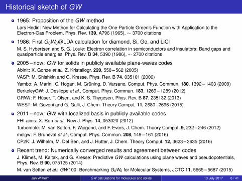
Historical sketch of GW

1965: Proposition of the GW methodLars Hedin: New Method for Calculating the One-Particle Green’s Function with Application to theElectron-Gas Problem, Phys. Rev. 139, A796 (1965), ∼ 3700 citations

1986: First G0W0@LDA calculation for diamond, Si, Ge, and LiClM. S. Hybertsen and S. G. Louie: Electron correlation in semiconductors and insulators: Band gaps andquasiparticle energies, Phys. Rev. B 34, 5390 (1986), ∼ 2700 citations

2005 – now: GW for solids in publicly available plane-waves codesAbinit: X. Gonze et al., Z. Kristallogr. 220, 558 – 562 (2005)VASP: M. Shishkin and G. Kresse, Phys. Rev. B 74, 035101 (2006)Yambo: A. Marini, C. Hogan, M. Grüning, D. Varsano, Comput. Phys. Commun. 180, 1392 – 1403 (2009)BerkeleyGW: J. Deslippe et al., Comput. Phys. Commun. 183, 1269 – 1289 (2012)GPAW: F. Hüser, T. Olsen, and K. S. Thygesen, Phys. Rev. B 87, 235132 (2013)WEST: M. Govoni and G. Galli, J. Chem. Theory Comput. 11, 2680 –2696 (2015)

2011 – now: GW with localized basis in publicly available codesFHI-aims: X. Ren et al., New J. Phys. 14, 053020 (2012)Turbomole: M. van Setten, F. Weigend, and F. Evers, J. Chem. Theory Comput. 9, 232 – 246 (2012)molgw: F. Bruneval et al., Comput. Phys. Commun. 208, 149 – 161 (2016)CP2K: J. Wilhelm, M. Del Ben, and J. Hutter, J. Chem. Theory Comput. 12, 3623 – 3635 (2016)

Recent trend: Numerically converged results and agreement between codesJ. Klimeš, M. Kaltak, and G. Kresse: Predictive GW calculations using plane waves and pseudopotentials,Phys. Rev. B 90, 075125 (2014)M. van Setten et al.: GW100: Benchmarking G0W0 for Molecular Systems, JCTC 11, 5665 – 5687 (2015)








7 Summary


Hedin’s equations

Hedin’s equation: Complicated self-consistent equations which give the exact self-energy.

Notation: (1) = (r1, t1), G0: non-interacting Green’s function, e.g. from DFT

Self-energy: Σ(1, 2) = i∫

d(34)G(1, 3)Γ(3, 2, 4)W (4, 1+)

Green’s function: G(1, 2) = G0(1, 2) +

∫d(34)G0(1, 3)Σ(3, 4)G(4, 2)

Screened interaction: W (1, 2) = V (1, 2) +

∫d(34)V (1, 3)P(3, 4)W (4, 2)

Bare interaction: V (1, 2) = δ(t1 − t2)/|r1 − r2|

Polarization: P(1, 2) = −i∫

d(34)G(1, 3)G(4, 1+)Γ(3, 4, 2)

Vertex function: Γ(1, 2, 3) = δ(1, 2)δ(1, 3) +

∫d(4567)

∂Σ(1, 2)

∂G(4, 5)G(4, 6)G(7, 5)Γ(6, 7, 3)

It can be shown that Σ(r1, t1, r2, t2)=Σ(r1, r2, t2 − t1). After a Fourier transform of Σ fromtime t ≡ t2 − t1 to frequency (= energy), the self-energy Σ(r, r′, ω) can be used to computethe quasiparticle levels εn using(

−∇2

2+ vel-core(r) + vH(r)

)ψn(r) +

∫dr′ Σ(r, r′, εn)ψn(r′) = εn ψn(r)


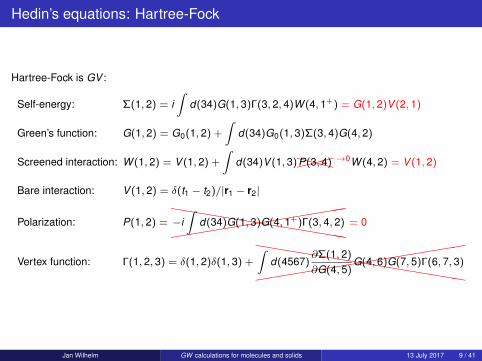
Hedin’s equations: Hartree-Fock

Hartree-Fock is GV :


d(34)G(1, 3)Γ(3, 2, 4)W (4, 1+) = G(1, 2)V (2, 1)


∫d(34)G0(1, 3)Σ(3, 4)G(4, 2)


∫d(34)V (1, 3)��XXXP(3, 4) →0W (4, 2) = V (1, 2)


Polarization: P(1, 2) =((((

((((((((

((hhhhhhhhhhhhhh−i∫

d(34)G(1, 3)G(4, 1+)Γ(3, 4, 2) = 0


((((((((

(((((((

(hhhhhhhhhhhhhhhh

∫d(4567)

∂Σ(1, 2)

∂G(4, 5)G(4, 6)G(7, 5)Γ(6, 7, 3)


Hedin’s equations: GW


d(34)G(1, 3)Γ(3, 2, 4)W (4, 1+) = iG(1, 2)W (2, 1+)


∫d(34)G0(1, 3)Σ(3, 4)G(4, 2)


∫d(34)V (1, 3)P(3, 4)W (4, 2)


Polarization: P(1, 2) = −i∫

d(34)G(1, 3)G(4, 1+)��XXXXΓ(3, 4, 2) = G(1, 2)G(2, 1+)


((((((((

(((((((

(hhhhhhhhhhhhhhhh

∫d(4567)

∂Σ(1, 2)

∂G(4, 5)G(4, 6)G(7, 5)Γ(6, 7, 3)


Screening

In GW , the screened Coulomb interaction is appearing:

W (r, r′, ω) =

∫dr′′ε−1(r, r′′, ω)v(r′′, r′)

where v(r, r′) = 1/|r− r′|.

Compare to screened Coulomb potential with local and static [ε(r, r′, ω) = εrδ(r− r′)]dielectric function using the dielectric constant εr (in SI units):

W (r, r′) =1

4πε0εr

1|r− r′|

screening

charge which has been added to the system

internal mobile charge carriers (e.g. electrons) which adapt due to the + charge

screening: adaption of electrons due to additional charge, key ingredient in GW (next slide)


V in Hartree-Fock versus W in GW

Gedankenexperiment: Ionization which leads to a hole (marked by "+")

εHOMO

εLUMO

Energy

εLUMO+1

εvac=0

εHOMO-1

Hartree-Fock: Σ=GV GW : Σ=GW

screening ("W ")no screening ("V ")

HF does not account for relaxation of electrons after adding an electron to an unoccupied MOor removing an electron from an occupied MO (only V in HF, no W or ε)⇒ occupied levels are too low, unoccupied levels are too high⇒ HOMO-LUMO gap too largeIn DFT, εn (besides εHOMO) do not have any physical meaning. Self-interaction error (SIE) incommon GGA functionals⇒ HOMO far too high in DFT⇒ HOMO-LUMO gap too low in DFTMixing HF and DFT (hybrids) can give accurate HOMO-LUMO gaps since two errors (SIE inDFT vs. absence of screening in HF) may compensateGW accounts for screening (since W is included) after adding an electron to an unoccupiedMO or removing an electron from an occupied MO⇒ accurate εGW

n


Physics beyond GW

GW does not account for the exact adaption of other electrons⇒ εGW

n can be improved by higher level of theory ("adding more diagrams")

Analogy: Full CI contains all determinants (= diagrams), but is untractable for large systems.Way out: neglect unnecessary determinants leading to e.g. CCSD, CCSD(T), RPA, MP2

Exact expansion of the self-energy:

Σ(1, 2) = iG(1, 2)W (2, 1+)−∫

d(34) G(1, 3)W (1, 4)G(4, 2)W (3, 2)G(3, 4) + . . .

⇒ GW approximation is good if W is small, otherwise higher order terms in W important

Screening is high in systems with small bandgap (since MOs in occupied orbitals can scatterinto unoccupied orbitals with low loss of energy)

⇒ ε is large in systems with small bandgap

⇒W is small in systems with small bandgap

⇒ The GW approximation is good for systems with small bandgaps








7 Summary


Accuracy of G0W0

Benchmark for solids (VASP)

Bandgap = HOMO-LUMO gap

Liu et al., PRB 94, 165109 (2016)

Benchmark for molecules (FHI-aims)

MAE = Mean absolute errorIP = Ionization potential = |εHOMO|

EA = Electron affinity = |εLUMO|Knight et al., JCTC 12, 615 (2016)


Application of G0W0 to periodic graphene nanoribbons

AGNR7

AGNR4

AGNR5

AGNR6

L. Yang, C.-H. Park, Y.-W. Son, M. L. Cohen, and S. G. Louie, Phys. Rev. Lett. 99, 186801 (2007)


Application of G0W0 to novel graphene nanoribbons

S. Wang, L. Talirz, C. A. Pignedoli, X. Feng, K. Müllen, R. Fasel, P. Ruffieux,Nat. Commun. 7, 11507 (2016)


Application of G0W0 to novel perovskite solar cells

M. R. Filip, G. E. Eperon, H. J. Snaith, and F. Giustino, Nat. Commun. 5, 5757 (2014)








7 Summary

Literature: J. Wilhelm, M. Del Ben, and J. Hutter, J. Chem. Theory Comput. 12, 3623 – 3635 (2016)


Resolution of the identity (RI) [Chem. Phys. Lett. 213, 514-518 (1993)]

In post-DFT methods as GW , four-index Coulomb integrals are appearing:

(nm|kl) =

∫d3r d3r′ψn(r)ψm(r)

1|r− r′| ψk (r′)ψl (r′)

RI with overlap metric

Id =∑PQ

|P〉S−1PQ 〈Q|

(nm|kl) =∑

PQRT

(nmP)S−1PQ VQRS−1

RT (Tkl)

(nmP) =

∫d3rψn(r)ψm(r)ϕP(r)

Resolution of the identity basis {ϕP} with

Overlap matrix

SPQ =∫

d3r ϕP(r)ϕQ(r)

Coulomb matrix

VPQ =∫

d3r d3r′ ϕP(r)ϕQ(r′)/|r− r′|

RI with Coulomb metric

Id =∑PQ

|P〉V−1PQ 〈Q|

1r̂

(nm|kl) =∑

PQRT

(nm|P)V−1PQ VQRV−1

RT (T |kl)

=∑PQ

(nm|P)V−1PQ (Q|kl)

=∑PQR

(nm|P)V−1/2PQ︸︷︷︸

= BnmQ

V−1/2QR (R|kl)︸︷︷︸

= BklQ

=∑

Q

BnmQ Bkl

Q

(nm|P) =

∫d3r d3r′ψn(r)ψm(r)

1|r− r′| ϕP(r′)


G0W0 in real space versus GW with RI

G0W0 in real space

1 Compute density response [O(N4)]

χ(r, r′, iω)=∑

ia

ψa(r′)ψi (r′)ψi (r)ψa(r)2(εi − εa)

ω2 + (εi − εa)2

2 Compute dielectric function

ε(r, r′, iω) = δ(r, r′)−∫

dr′′v(r, r′′)χ(r′′, r′, iω)


W0(r, r′, iω) =

∫dr′′ε−1(r, r′′, iω)v(r′′, r′)

4 Compute self-energy (SE)

Σ(r, r′, iω) = −∞∫−∞

dω′

2πG0(r, r′, iω−iω′)W0(r, r′, iω′)

5 Compute G0W0 quasiparticle energies

εG0W0n = εn + 〈ψn|Re Σ(ε

G0W0n )− vxc|ψn〉

G0W0 with RI1 Compute ΠPQ matrix [Π equivalent to

v1/2χv1/2, O(N4) operations]

ΠPQ(iω) =∑

ia

BiaP

2(εi − εa)

ω2 + (εi − εa)2 BiaQ

2 Compute symmetrized dielectric function

εPQ(iω) = δPQ − ΠPQ(iω)

3 Compute SE Σn(iω) ≡ 〈ψn|Σ(iω)|ψn〉

Σn(iω) =−∞∫−∞

dω′

2π

all∑m

1i(ω − ω′) + εF − εm

×∑PQ

BnmP ε−1

PQ (iω′)BmnQ





Exchange and correlation self-energy

The self-energy Σn(iω) from the last slide,

Σn(iω) =−∞∫−∞

dω′

2π

all∑m

1i(ω − ω′) + εF − εm

∑PQ

BnmP ε−1

PQ (iω′)BmnQ ,

is split into an exchange part Σxn [= (n, n)-diagonal element of the Fock matrix]

Σxn = −

occ∑m

∑P

BnmP Bmn

P ,

and a correlation part

Σcn(iω) =−

∞∫−∞

dω′

2π

all∑m

1i(ω − ω′) + εF − εm

∑PQ

BnmP [ε−1

PQ (iω′)−δPQ ]BmnQ ,

such that Σn(iω) = Σxn + Σc

n(iω). This procedure guarantees numerical stability.


Analytic continuation

The self-energy Σcn(iω) is computed for imaginary frequency and needed for real frequency

(= energy) for solving the quasiparticle equation:

εG0W0n = εn + Re Σn(ε

G0W0n )− vxc

n

where vxcn =

∫d3rψn(r)vxc(r)ψn(r).

Σn(ω) for a real-valued ω is obtained from Σn(iω) by fitting an N-point Padé approximant

P(iω) =

N−1∑j=0

aj · (iω)j

1 +N∑

k=0bk · (iω)k

to Σn(iω) to determine the complex numbers aj and bk . Then, Σn(ω) is obtained by evaluating P:

Σn(ω) =

N−1∑j=0

aj · (ω − εF)j

1 +N∑

k=0bk · (ω − εF)k

where the Fermi level εF appears to obtain the correct offset.


Input for G0W0@PBE for the H2O molecule I

DFT calculation to get the molecular orbitals ψn from a PBE calculation:

&FORCE_EVALMETHOD Quickstep&DFTBASIS_SET_FILE_NAME BASIS_def2_QZVP_RI_ALLPOTENTIAL_FILE_NAME POTENTIAL&MGRID

CUTOFF 400REL_CUTOFF 50

&END MGRID&QS

! all electron calculation since GW100! is all-electron testMETHOD GAPW

&END QS&POISSON

PERIODIC NONEPSOLVER MT

&END&SCF

EPS_SCF 1.0E-6SCF_GUESS ATOMICMAX_SCF 200

&END SCF&XC

&XC_FUNCTIONAL PBE&END XC_FUNCTIONAL! GW is part of the WF_CORRELATION section&WF_CORRELATION

...&END

&END XC&END DFT ...

&SUBSYS&CELLABC 10.0 10.0 10.0PERIODIC NONE

&END CELL&COORDO 0.0000 0.0000 0.0000H 0.7571 0.0000 0.5861H -0.7571 0.0000 0.5861

&END COORD&TOPOLOGY&CENTER_COORDINATES&END

&END TOPOLOGY&KIND H! def2-QZVP: basis of GW100BASIS_SET def2-QZVP! just very large RI basis to ensure good! convergence in RI basisRI_AUX_BASIS RI-5ZPOTENTIAL ALL

&END KIND&KIND OBASIS_SET def2-QZVPRI_AUX_BASIS RI-5ZPOTENTIAL ALL

&END KIND&END SUBSYS

&END FORCE_EVAL&GLOBALRUN_TYPE ENERGYPROJECT ALL_ELECPRINT_LEVEL MEDIUM

&END GLOBAL


Input for G0W0@PBE for the H2O molecule II

Parameters for the GW calculation:

&XC

&XC_FUNCTIONAL PBE&END XC_FUNCTIONAL

! GW is part of the WF_CORRELATION section&WF_CORRELATION

! RPA is used to compute the density response functionMETHOD RI_RPA_GPW

! Use Obara-Saika integrals instead of GPW integrals! since OS is much fasterERI_METHOD OS

&RI_RPA

! use 100 quadrature points to perform the! frequency integration in GWRPA_NUM_QUAD_POINTS 100

! SIZE_FREQ_INTEG_GROUP is a group size for! parallelization and should be increased for! large calculations to prevent out of memory.! maximum for SIZE_FREQ_INTEG_GROUP! is the number of MPI tasksSIZE_FREQ_INTEG_GROUP 1

GW

...

&RI_G0W0

! compute the G0W0@PBE energy of HOMO-9,! HOMO-8, ... , HOMO-1, HOMOCORR_OCC 10

! compute the G0W0@PBE energy of LUMO,! LUMO+1, ... , LUMO+20CORR_VIRT 20

! Pade approximantANALYTIC_CONTINUATION PADE

! for solving the quasiparticle equation,! the Newton method is used as in GW100CROSSING_SEARCH NEWTON

! use RI for the exchange self-energyRI_SIGMA_X

&END RI_G0W0

&END RI_RPA

! NUMBER_PROC is a group size for! parallelization and should be increased! for large calculationsNUMBER_PROC 1

&END WF_CORRELATION

&END XC


Basis set convergence for benzene: HOMO level

1∞

1816

cc-5

ZVP

1504

cc-Q

ZVP

1258

cc-T

ZVP

1108

cc-D

ZVP

– 9.4

– 9.2

– 9.0

– 8.8

– 8.6

– 8.4

1/Nprimary basis functions

G0W

0@

PB

E0

HO

MO

(eV

)

Basis set extrapolationG0W0@PBE0 HOMO

linear fit

aug-

5ZV

P

aug-

QZV

P

aug-

TZV

P

aug-DZVP

Slow basis set convergence for the HOMO level

Basis set extrapolation necessary


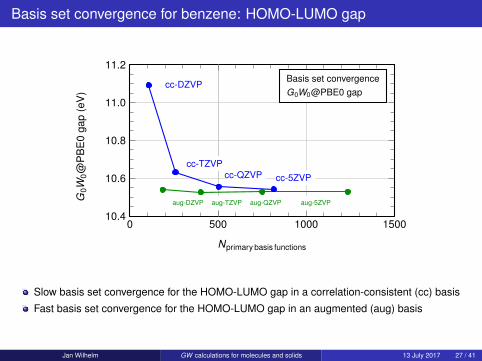
Basis set convergence for benzene: HOMO-LUMO gap

0 500 1000 150010.4

10.6

10.8

11.0

11.2

cc-DZVP

cc-TZVPcc-QZVP cc-5ZVP

aug-DZVP aug-TZVP aug-QZVP aug-5ZVP

Nprimary basis functions

G0W

0@

PB

E0

gap

(eV

)Basis set convergenceG0W0@PBE0 gap

Slow basis set convergence for the HOMO-LUMO gap in a correlation-consistent (cc) basis

Fast basis set convergence for the HOMO-LUMO gap in an augmented (aug) basis


Computational cost for water in a cc-TZVP basis

32 64 96 128 160100

101

102

103

104

Number of water molecules

Exe

cutio

ntim

e(c

ore

hour

s) overall G0W 0 calc.computing ΠPQ(iω)

fit (exponent: 3.93)

O(N4) computational cost as expected

massively parallel implementation








7 Summary

Literature: J. Wilhelm and J. Hutter, Phys. Rev. B 95, 235123 (2017)


Motivation: Slow convergence of GW with the cell size

64

2×2×2

216

3×3×3

512

4×4×4

1000 3000 10000 30000 1000004.0

5.0

6.0

7.0

8.0

9.0

Natoms per cell

G0W

0@

PB

EH

OM

O-L

UM

Oga

p(e

V)

Solid LiHwithout correction

theoretical extrapolation

extrapolated value

with correctionLiH unit cell(1×1×1)

Very slow convergence of the G0W0 HOMO-LUMO gap as function of the cell size

The extrapolation (blue line) can be done with 1/N1/3atoms per cell

Comparison: Convergence of DFT gap with exp(−Natoms per cell) for non-metallic systems


1/L convergence of the HOMO-LUMO gap

1∞

13√4096

4×4×4

13√512

3×3×3

13√216

13√64

2×2×2

4.0

5.0

6.0

7.0

8.0

9.0

1/N 1/3atoms per cell (∼ 1/L)

G0W

0@

PB

EH

OM

O-L

UM

Oga

p(e

V)

Solid LiHcalculations

linear fit


Benchmark calculations for solids

(a)

1∞

116

4×4×4

18

3×3×3

16

14

2×2×2

4.0

5.0

6.0

7.0

8.0

9.0


G0W

0@

PB

Ega

p(e

V)

without correction linear fit extrapolated value with correction

1∞

116

4×4×4

18

3×3×3

16

14

2×2×2

4.0

5.0

6.0

7.0

8.0

9.0


G0W

0@

PB

Ega

p(e

V)

Solid LiH, exp. gap: 4.99 eV

l

1∞

116

18

16

14

5.0

6.0

7.0

8.0

9.0

10.0


Diamond, exp. gap: 5.48 eV

1∞

13√432

13√128

13√16

7.0

8.0

9.0

10.0

11.0

12.0


G0W

0@

PB

Ega

p(e

V)

NH3 crystal

l

1∞

13√324

13√96

13√12

9.0

10.0

11.0

12.0

13.0

14.0


CO2 crystal


Input for periodic G0W0@PBE for solid LiH

...&XC

&XC_FUNCTIONAL PBE&END XC_FUNCTIONAL

&WF_CORRELATION

METHOD RI_RPA_GPW

&RI_RPA

RPA_NUM_QUAD_POINTS 100

GW

&RI_G0W0

CORR_OCC 5CORR_VIRT 5

! activate the periodic correctionPERIODIC

ANALYTIC_CONTINUATION PADE

CROSSING_SEARCH NEWTON

&END RI_G0W0

...

! HF calculation for the exchange self-energy! Here, the truncation of the Coulomb operator works&HF

&SCREENINGEPS_SCHWARZ 1.0E-6SCREEN_ON_INITIAL_P TRUE

&END

&INTERACTION_POTENTIALPOTENTIAL_TYPE TRUNCATED! the truncation radius is half the cell sizeCUTOFF_RADIUS 2.00T_C_G_DATA t_c_g.dat

&END

&MEMORYMAX_MEMORY 0

&END

&END

&END RI_RPA

NUMBER_PROC 1

&END

&END XC

...








7 Summary

Literature: J. Wilhelm, D. Golze, C. A. Pignedoli, and J. Hutter, in preparation


O(N3) GW space-time method [Rojas et al., PRL 74, 1827 (1995)]

Canonical O(N4) G0W0

1 Compute density response in O(N4)

χ(r, r′, iω)=∑

ia

ψa(r′)ψi (r′)ψi (r)ψa(r)2(εi − εa)

ω2 + (εi − εa)2


ε(r, r′, iω) = δ(r, r′)−∫

dr′′v(r, r′′)χ(r′′, r′, iω)


W0(r, r′, iω) =

∫dr′′ε−1(r, r′′, iω)v(r′′, r′)

4 Compute self-energy

Σ(r, r′, iω) = −∞∫−∞

dω′

2πG0(r, r′, iω−iω′)W0(r, r′, iω′)




O(N3) G0W0 space-time method

1 Compute density response in O(N3)

χ(r, r′, iτ)=∑

ia

ψa(r′)ψi (r′)ψi (r)ψa(r)e−(εa−εi )τ

=occ∑

iψi (r′)ψi (r)e−|(εi−εF)τ| virt∑

aψa(r′)ψa(r)e−|(εa−εF)τ|


ε(r, r′, iτ) = δ(r, r′)−∫

dr′′v(r, r′′)χ(r′′, r′, iτ)


W0(r, r′, iω) =

∫dr′′ε−1(r, r′′, iω)v(r′′, r′)

4 Compute self-energy

Σ(r, r′, iτ) = −G0(r, r′, iτ)W0(r, r′, iτ)





Resolution of the identity (RI) II

RI with overlap metric

(µν|λσ) =∑

PQRT

(µνP)S−1PQ VQRS−1

RT (Tλσ)

(µνP) =

∫d3rφµ(r)φν(r)ϕP(r)

(νµP) = 0 if one of φµ, φν , ϕP far-off

slightly larger RI basis as for RI-Coulomb

RI with Coulomb metric

(µν|λσ) =∑PQ

(µν|P)V−1PQ (Q|λσ)

(µν|P) =

∫d3r d3r′φµ(r)φν(r)

1|r− r′| ϕP(r′)

(νµ|P) = 0 if φµ, φν far-off

No sparsity of (νµ|P) if ϕP far-off

ϕQ(r)

φν(r)φµ(r)

l(µνP) =

∫d3rφµ(r)φν(r)ϕP(r) ≈ 0 (µν|P) =

∫d3r d3r′φµ(r)φν(r)

1|r− r′| ϕP(r′) ≈ 1


Cubic-scaling GW in a Gaussian basis with overlap-metric RI

Gµν(iτ) =

{ ∑i Cµi Cν i e−|(εi−εF)τ | , if τ < 0

−∑a CµaCνae−|(εa−εF)τ | , if τ > 0

χ̃PQ(iτ) =∑µσ

∑λ

(λσP)Gµλ(iτ)

×∑ν

(µνQ)Gνσ(−iτ)

O(N2), JW, P. Seewald, M. Del Ben,J. Hutter, JCTC 12, 5851 – 5859 (2016)

χ(iτ) = S−1χ̃(iτ)S−1

χ(iω)

ε(iω) = 1− Vχ(iω)

W(iω) = ε−1(iω)V

W̃(iω) = S−1W(iω)S−1

W̃(iτ)

Σn(iτ) = − ∑µνPQ

Gµν(iτ)(nµP)

×W̃PQ(iτ)(Qνn)

O(N2NGW )

Σn(iω)

Σn(ε)

εG0W0n = εn + Re Σn(ε

G0W0n )− vxc

n

RI with overlap metric: (µν|λσ) =∑

PQRT(µνP)S−1

PQ VQRS−1RT (Tλσ)


Computational scaling of cubic-scaling GW

114(7,12)

222(7,24)

438(7,48)

870(7,96)

1734(7,192)

100

101

102

103

104

105

Number of atoms (Name of the GNR)

Exe

cutio

ntim

e(n

ode

hour

s) O(N4) G0W0 total fit: O(N 3.80)O(N3) G0W0 total fit: O(N 2.13)O(N 3) steps fit: O(N 2.84)

Cubic-scaling GW particularly efficient for systems withlow dimensionality (best: one-dimensional chain, worst: spherical molecule, periodic system)local electronic structure (best: solution of small molecules, worst: extended π system)

(7,12) GNR (7,24) GNRAGNR7


Input for cubic-scaling G0W0

G0W0@PBE for the (7,192) GNR (1734 atoms, aug-DZVP basis)

400 Piz Daint MC nodes (4 OMP threads)

&WF_CORRELATION

METHOD RI_RPA_GPW

! cubic-scaling GW only works with overlap metric RIRI OVERLAP

ERI_METHOD OS

&WFC_GPW

! EPS_FILTER should be tuned, computational cost! strongly depends on EPS_FILTEREPS_FILTER 1.0E-9

! EPS_GRID may be tuned since memory is weakly! dependent on itEPS_GRID 1.0E-6

&END

&RI_RPA

! cubic-scaling GW only works with the minimax grid! in imag. time and frequencyMINIMAX

! number of time and frequency points, at most 20RPA_NUM_QUAD_POINTS 12

IM_TIME

...

! parameters for computing chi(it)&IM_TIME

! EPS_FILTER_IM_TIME should be tunedEPS_FILTER_IM_TIME 1.0E-11

! for large systems, increase GROUP_SIZE_3C! to prevent out of memory (OOM)GROUP_SIZE_3C 9

! for large systems, increase GROUP_SIZE_3C! to prevent out of memory (OOM)GROUP_SIZE_P 1

! for larger systems, MEMORY_CUT must be! increased to prevent out of memory (OOM)MEMORY_CUT 12

GW

&END

&RI_G0W0CORR_OCC 15CORR_VIRT 15CROSSING_SEARCH NEWTONOMEGA_MAX_FIT 1.0ANALYTIC_CONTINUATION PADERI OVERLAPRI_SIGMA_X

&END RI_G0W0&END RI_RPA

&END








7 Summary


Summary

GW : method to compute quasiparticle energiesfrom first principles

Accuracy of G0W0@PBE for solids, G0W0@PBE0for molecules in the order of few hundreds of meV

High O(N4) computational cost

Hundreds of atoms can be treated onsupercomputers by G0W0 in CP2K

Slow basis set convergence

Correction scheme for periodic G0W0 calculations

O(N3) G0W0 method for big systems

εHOMO

εLUMO

Energy

εLUMO+1

εvac=0

εHOMO-1

Quasiparticle energies of aclosed shell molecule


Date post:	03-May-2018
Category:	Documents
Upload:	dangliem
View:	219 times
Download:	1 times

GW calculations for molecules and solids: Theory and ...2017_uzh_cp2k-tutorial:... · GW...

Documents