Gyroharmonic Analysis on Relativistic Gyrogroups › bitstream › 10400.8 › ... · ourierF...

Gyroharmonic Analysis on Relativistic Gyrogroups ∗

Milton Ferreira

School of Technology and Management,

Polytechnic Institute of Leiria, Portugal

2411-901 Leiria, Portugal.

Email: [email protected]

and

Center for Research and Development in Mathematics and Applications (CIDMA),

University of Aveiro, 3810-193 Aveiro, Portugal.

Email [email protected]

Abstract

Einstein, Möbius, and Proper Velocity gyrogroups are relativistic gyrogroups thatappear as three di�erent realizations of the proper Lorentz group in the real Minkowskispace-time Rn,1. Using the gyrolanguage we study their gyroharmonic analysis. Al-though there is an algebraic gyroisomorphism between the three models we showthat there are some di�erences between them. Our study focus on the translationand convolution operators, eigenfunctions of the Laplace-Beltrami operator, Poissontransform, Fourier-Helgason transform, its inverse, and Plancherel's Theorem. Weshow that in the limit of large t, t→ +∞, the resulting gyroharmonic analysis tendsto the standard Euclidean harmonic analysis on Rn, thus unifying hyperbolic andEuclidean harmonic analysis.

Keywords: Gyrogroups, Gyroharmonic Analysis, Laplace Beltrami operator, Eigenfunc-tions, Generalized Helgason-Fourier transform, Plancherel's Theorem.

1 Introduction

Harmonic analysis is the branch of mathematics that studies the representation of functionsor signals as the superposition of basic waves called harmonics. Closely related is the studyof Fourier series and Fourier transforms. Its applications are of major importance and canbe found in diverse areas such as signal processing, quantum mechanics, and neuroscience(see [23] for an overview). The classical Fourier transform on Rn is still an area of research,particularly concerning Fourier transformation on more general objects such as tempereddistributions. Some of its properties can be translated in terms of the Fourier transform.For instance, the Paley-Wiener theorem states that if a function is a nonzero distributionof compact support then its Fourier transform is never compactly supported [22]. Thisis a very elementary form of an uncertainty principle in the harmonic analysis setting.Fourier series can be conveniently studied in the context of Hilbert spaces, which providesa connection between harmonic analysis and functional analysis.

In the last century the Fourier transform was generalised to compact groups, abelianlocally compact groups, symmetric spaces, etc.. For compact groups, the Peter-Weyl the-orem establish the relationship between harmonics and irreducible representations. This

∗Accepted author's manuscript (AAM) published in [Mathematics Interdisciplinary Research, 1 (2016),69-109]. The �nal publication is available at http://mir.kashanu.ac.ir/article_13908.html

1

http://mir.kashanu.ac.ir/article_13908.html

choice of harmonics enjoys some of the useful properties of the classical Fourier transformin terms of carrying convolutions to pointwise products, or otherwise showing a certainunderstanding of the underlying group structure. For general nonabelian locally compactgroups, harmonic analysis is closely related to the theory of unitary group representations.Noncommutative harmonic analysis appeared mainly in the context of symmetric spaceswhere many Lie groups are locally compact and noncommutative. These examples are ofinterest and frequently applied in mathematical physics, and contemporary number theory,particularly automorphic representations. The development of noncommutative harmonicanalysis was done by many mathematicians like John von Neumann, Harisch-Chandra andSigurdur Helgason [13, 14].

It is well-known that Fourier analysis is intimately connected with the action of thegroup of translations on Euclidean space. The group structure enters into the study ofharmonic analysis by allowing the consideration of the translates of the object under study(functions, measures, etc.). First we study the spectral analysis �nding the elementarycomponents for the decomposition and second we perform the harmonic or spectral syn-thesis, �nding a way in which the object can be construed as a combination of its elementarycomponents [16]. Harmonic analysis in Euclidean spaces is rich because of its connectionwith several classes of transformations: the dilations and the rotations as well as the trans-lations. The Fourier transform in Rn has a very simple transformation law under dilationsand it commutes with the action of rotations.

The real hyperbolic space is commonly viewed as a homogeneous space obtained fromthe quotient SO0(n, 1)/SO(n) where SO0(n, 1) is the proper Lorentz group in the Minkowskispace Rn,1 and SO(n) is the special orthogonal group. It is well known that pure Lorentztransformations (the translations in hyperbolic space) do not form a group since the com-position of two is no longer a pure Lorentz transformation. However, by incorporating thegyration operator it is possible to obtain a gyroassociative law. The resulting algebraicstructure called gyrogroup by A.A. Ungar [25] repairs the breakdown of associativity andcommutativity of the relativistic additions. The gyrogroup structure is a natural extensionof the group structure, discovered in 1988 by A. A. Ungar in the context of Einstein'svelocity addition law [24, 25]. It has been studied by A. A. Ungar and others see, for in-stance, [26, 8, 6, 27, 29, 30]. Gyrogroups provide a fruitful bridge between nonassociativealgebra and hyperbolic geometry, just as groups lay the bridge between associative algebraand Euclidean geometry.

In this survey paper we show the similarities and di�erences between gyroharmonicanalysis on three relativistic gyrogroups: Möbius, Einstein, and Proper Velocity gyrogroups.For the Möbius and Eintein cases we provide a generalization of the results in [9, 10]by replacing the real parameter σ by a complex parameter z, under the identi�cation2z = n+ σ − 2, where n is the dimension of the hyperbolic space.

The paper is organized as follows. In Section 2 we review harmonic analysis on Rn asspectral theory of the Laplace operator. In Sections 3, 4, and 5 we present the results con-cerning gyroharmonic analysis for the Einstein, Möbius, and Proper Velocity gyrogroups,respectively. Each of these sections focus the following aspects: the relativistic additionand its properties, the generalised translation operator and the associated convolution op-erator, the eigenfunctions of the generalised Laplace-Beltrami operator, the generalizedspherical functions, the generalized Poisson transform, the generalized Helgason Fouriertransform, its inverse and Plancherel's Theorem. We show that in the limit t → +∞ werecover the well-known results in Euclidean harmonic analysis. Two appendices, A and B,concerning all necessary facts on spherical harmonics and Jacobi functions, are found atthe end of the paper.

2

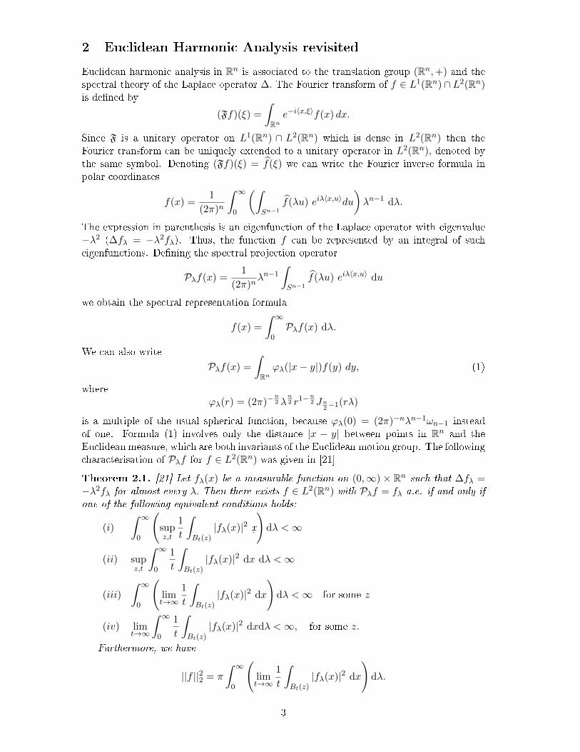
2 Euclidean Harmonic Analysis revisited

Euclidean harmonic analysis in Rn is associated to the translation group (Rn,+) and thespectral theory of the Laplace operator ∆. The Fourier transform of f ∈ L1(Rn)∩L2(Rn)is de�ned by

(Ff)(ξ) =

∫Rne−i〈x,ξ〉f(x) dx.

Since F is a unitary operator on L1(Rn) ∩ L2(Rn) which is dense in L2(Rn) then theFourier transform can be uniquely extended to a unitary operator in L2(Rn), denoted bythe same symbol. Denoting (Ff)(ξ) = f(ξ) we can write the Fourier inverse formula inpolar coordinates

f(x) =1

(2π)n

∫ ∞0

(∫Sn−1

f(λu) eiλ〈x,u〉du

)λn−1 dλ.

The expression in parenthesis is an eigenfunction of the Laplace operator with eigenvalue−λ2 (∆fλ = −λ2fλ). Thus, the function f can be represented by an integral of sucheigenfunctions. De�ning the spectral projection operator

Pλf(x) =1

(2π)nλn−1

∫Sn−1

f(λu) eiλ〈x,u〉 du

we obtain the spectral representation formula

f(x) =

∫ ∞0Pλf(x) dλ.

We can also write

Pλf(x) =

∫Rnϕλ(|x− y|)f(y) dy, (1)

whereϕλ(r) = (2π)−

n2 λ

n2 r1−

n2 Jn

2−1(rλ)

is a multiple of the usual spherical function, because ϕλ(0) = (2π)−nλn−1ωn−1 insteadof one. Formula (1) involves only the distance |x − y| between points in Rn and theEuclidean measure, which are both invariants of the Euclidean motion group. The followingcharacterisation of Pλf for f ∈ L2(Rn) was given in [21]

Theorem 2.1. [21] Let fλ(x) be a measurable function on (0,∞) × Rn such that ∆fλ =−λ2fλ for almost every λ. Then there exists f ∈ L2(Rn) with Pλf = fλ a.e. if and only ifone of the following equivalent conditions holds:

(i)

∫ ∞0

(supz,t

1

t

∫Bt(z)

|fλ(x)|2 x.

)dλ <∞

(ii) supz,t

∫ ∞0

1

t

∫Bt(z)

|fλ(x)|2 dx dλ <∞

(iii)

∫ ∞0

(limt→∞

1

t

∫Bt(z)

|fλ(x)|2 dx

)dλ <∞ for some z

(iv) limt→∞

∫ ∞0

1

t

∫Bt(z)

|fλ(x)|2 dxdλ <∞, for some z.

Furthermore, we have

||f ||22 = π

∫ ∞0

(limt→∞

1

t

∫Bt(z)

|fλ(x)|2 dx

)dλ.

3

3 Gyroharmonic analysis on the Einstein gyrogroup

3.1 Einstein addition in the ball

The Beltrami-Klein model of the n−dimensional real hyperbolic geometry can be realisedas the open ball Bnt = {x ∈ Rn : ‖x‖ < t} of Rn, endowed with the Riemannian metric

ds2 =‖dx‖2

1− ‖x‖2

t2

+(〈x, dx〉)2

t2(

1− ‖x‖2

t2

)2 .This metric corresponds to the metric tensor

gij(x) =δij

1− ‖x‖2

t2

+xixj

t2(

1− ‖x‖2

t2

)2 , i, j ∈ {1, . . . , n}

and its inverse is given by

gij(x) =

(1− ‖x‖

2

t2

)(δij −

xixjt2

), i, j ∈ {1, . . . , n}.

The group of all isometries of the Klein model [34] consists of the elements of the groupO(n) and the mappings given by

Ta(x) =a+ Pa(x) + µaQa(x)

1 + 1t2〈a, x〉

(2)

where

Pa(x) =

{〈a, x〉 a

‖a‖2 if a 6= 0

0 if a = 0, Qa(x) = x− Pa(x), and µa =

√1− ‖a‖

2

t2.

Some properties are listed in the next proposition.

Proposition 3.1. Let a ∈ Bnt . Then

(i) P 2a = Pa, Q2

a = Qa, 〈a, Pa(x)〉 = 〈a, x〉 , and 〈a,Qa(x)〉 = 0.

(ii) Ta(0) = a and Ta(−a) = 0.

(iii) Ta(T−a(x)) = T−a(Ta(x)) = x, ∀x ∈ Bnt .

(iv) Ta

(±t a‖a‖

)= ±t a

‖a‖. Moreover, Ta �xes two points on ∂Bnt and no point of Bnt .

(v) The identity

1− 〈Ta(x), Ta(y)〉t2

=

(1− ‖a‖

2

t2

)(1− 〈x,y〉

t2

)(

1 + 〈x,a〉t2

)(1 + 〈y,a〉

t2

) (3)

holds for all x, y ∈ Bnt . In particular, when x = y we have

1− ‖Ta(x)‖2

t2=

(1− ‖a‖

2

t2

)(1− ‖x‖

2

t2

)(

1 + 〈x,a〉t2

)2 (4)

and when x = 0 in (3) we obtain

1− 〈a, Ta(y)〉t2

=1− ‖a‖

2

t2

1 + 〈y,a〉t2

. (5)

4

(vi) For R ∈ O(n)R ◦ Ta = TRa ◦R. (6)

To endow the ball Bnt with a binary operation, closely related to vector addition in Rn,we de�ne the Einstein addition on Bnt by

a⊕ x := Ta(x), a, x ∈ Bnt . (7)

This de�nition agrees with Ungar's de�nition for the Einstein addition since we can write(2) as

a⊕ x =1

1 + 〈a,x〉t2

(a+

1

γax+

1

t2γa

1 + γa〈a, x〉 a

)(8)

where γa =

(√1− ‖a‖

2

t2

)−1is the relativistic gamma factor.

It is known that (Bnt ,⊕) is a gyrogroup (see [24, 27]), i.e., it satis�es the followingaxioms:

(G1) There is at least one element 0 satisfying 0⊕ a = a, for all a ∈ Bnt ;

(G2) For each a ∈ B there is an element a ∈ Bnt such that a⊕ a = 0;

(G3) For any a, b, c ∈ Bnt there exists a unique element gyr[a, b]c ∈ Bnt such that thebinary operation satis�es the left gyroassociative law

a⊕ (b⊕ c) = (a⊕ b)⊕ gyr[a, b]c; (9)

(G4) The map gyr[a, b] : Bnt → Bnt given by c 7→ gyr[a, b]c is an automorphism of (Bnt ,⊕);

(G5) The gyroautomorphism gyr[a, b] possesses the left loop property

gyr[a, b] = gyr[a⊕ b, b] (10)

for all a, b ∈ B.

The gyration operator can be given in terms of the Einstein addition ⊕ by the equation(see [27])

gyr [a, b]c = (a⊕ b)⊕ (a⊕ (b⊕ c)).

The Einstein gyrogroup is gyrocommutative since Einstein addition satis�es

a⊕ b = gyr [a, b](b⊕ a). (11)

In the limit t→ +∞, the ball Bnt expands to the whole of the space Rn, Einstein additionreduces to vector addition in Rn and, therefore, the gyrogroup (Bnt ,⊕) reduces to thetranslation group (Rn,+). Some useful gyrogroup identities ([27], pp. 48 and 68) that willbe used in this paper are

(a⊕ b) = (a)⊕ (b) (12)

a⊕ (a⊕ b) = b (13)

(gyr [a, b])−1 = gyr [b, a] (14)

gyr [a⊕ b,a] = gyr [a, b] (15)

gyr [a,b] = gyr [a, b] (16)

gyr [a,a] = I (17)

gyr [a, b](b⊕ (a⊕ c)) = (a⊕ b)⊕ c (18)

5

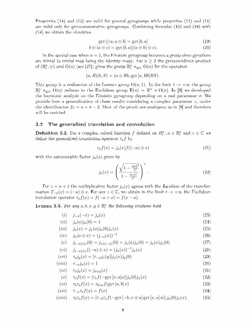
Properties (14) and (15) are valid for general gyrogroups while properties (12) and (18)are valid only for gyrocommutative gyrogroups. Combining formulas (15) and (18) with(14) we obtain the identities

gyr [a, a⊕ b] = gyr [b, a] (19)

b⊕ (a⊕ c) = gyr [b, a]((a⊕ b)⊕ c). (20)

In the special case when n = 1, the Einstein gyrogroup becomes a group since gyrationsare trivial (a trivial map being the identity map). For n ≥ 2 the gyrosemidirect productof (Bnt ,⊕) and O(n) (see [27]) gives the group Bnt ogyr O(n) for the operation

(a,R)(b, S) = (a⊕Rb, gyr [a,Rb]RS) .

This group is a realisation of the Lorentz group O(n, 1). In the limit t → +∞ the groupBnt ogyr O(n) reduces to the Euclidean group E(n) = Rn o O(n). In [9] we developedthe harmonic analysis on the Einstein gyrogroup depending on a real parameter σ. Weprovide here a generalization of these results considering a complex parameter z, underthe identi�cation 2z = n+ σ − 2. Most of the proofs are analogous as in [9] and thereforewill be omitted.

3.2 The generalised translation and convolution

De�nition 3.2. For a complex valued function f de�ned on Bnt , a ∈ Bnt and z ∈ C we

de�ne the generalised translation operator τaf by

τaf(x) = ja(x)f((−a)⊕ x) (21)

with the automorphic factor ja(x) given by

ja(x) =

√

1− ‖a‖2

t2

1− 〈a,x〉t2

z

. (22)

For z = n+ 1 the multiplicative factor ja(x) agrees with the Jacobian of the transfor-mation T−a(x) = (−a)⊕ x. For any z ∈ C, we obtain in the limit t→ +∞ the Euclideantranslation operator τaf(x) = f(−a+ x) = f(x− a).

Lemma 3.3. For any a, b, x, y ∈ Bnt the following relations hold

(i) j−a(−x) = ja(x) (23)

(ii) ja(a)ja(0) = 1 (24)

(iii) ja(x) = jx(a)ja(0)jx(x) (25)

(iv) ja(a⊕ x) = (j−a(x))−1 (26)

(v) j(−a)⊕x(0) = jx⊕(−a)(0) = jx(a)ja(0) = ja(x)jx(0) (27)

(vi) j(−a)⊕x((−a)⊕ x) = (ja(x))−1jx(x) (28)

(vii) τajy(x) = [τ−ajx(y)]jx(x)jy(0) (29)

(viii) τ−aja(x) = 1 (30)

(ix) τajy(x) = ja⊕y(x) (31)

(x) τaf(x) = [τxf(−gyr [x, a]a)]ja(0)jx(x) (32)

(xi) τbτaf(x) = τb⊕af(gyr [a, b]x) (33)

(xii) τ−aτaf(x) = f(x) (34)

(xiii) τbτaf(x) = [τ−bτxf(−gyr [−b, x⊕ a] gyr [x, a] a)] ja(0)jx(x). (35)

6

For the translation operator to be an unitary operator we have to properly de�ne aHilbert space. We consider the complex weighted Hilbert space L2(Bnt , dµz,t) with

dµz,t(x) =

(1− ‖x‖

2

t2

)z−n+12

dx,

where dx stands for the Lebesgue measure in Rn. For the special case z = 0 we recover theinvariant measure associated to the transformations Ta(x).

Proposition 3.4. For f, g ∈ L2(Bnt ,dµz,t) and a ∈ Bnt we have∫Bntτaf(x) g(x) dµz,t(x) =

∫Bntf(x) τ−ag(x) dµz,t(x). (36)

Corollary 3.5. For f, g ∈ L2(Bnt ,dµz,t) and a ∈ Bnt we have

(i)

∫Bntτaf(x) dµz,t(x) =

∫Bntf(x)j−a(x) dµz,t(x); (37)

(ii) If z = 0 then

∫Bntτaf(x) dµz,t(x) =

∫Bntf(x) dµz,t(x); (38)

(iii) ||τaf ||2 = ||f ||2. (39)

From Corollary 3.5 we see that the generalised translation τa is an unitary operator inL2(Bnt , dµz,t) and the measure dµz,t is translation invariant only for the case z = 0. Nowwe de�ne the generalised convolution of two functions in Bnt .

De�nition 3.6. The generalised convolution of two measurable functions f and g is givenby

(f ∗ g)(x) =

∫Bntf(y) τxg(−y) jx(x) dµz,t(y), x ∈ Bnt . (40)

By Proposition 3.4 and the change of variables −y 7→ z we can see that the generalisedconvolution is commutative, i.e., f ∗ g = g ∗ f. Before we prove that it is well de�ned forRe(z) < n−1

2 we need the following lemma.

Lemma 3.7. Let Re(z) < n−12 . Then∫

Sn−1

|jx(rξ) jx(x)| dσ(ξ) ≤ Cz

with

Cz =

1, if Re(z) ∈]− 1, 0[

Γ(n2

) (n−2Re(z)−12

)Γ(n−Re(z)

2

)Γ(n−Re(z)−1

2

) , if Re(z) ∈]−∞,−1] ∪ [0, n−12 [. (41)

Proof. Using (A.2) in Appendix A we obtain∫Sn−1

|jx(rξ) jx(x)| dσ(ξ) = 2F1

(Re(z)

2,Re(z) + 1

2;n

2;r2‖x‖2

t4

).

7

Considering the function g(s) = 2F1

(Re(z)

2 , Re(z)+12 ; n2 ; s

)and applying (A.8) and (A.6) in

Appendix A we get

g′(s) =Re(z)(Re(z) + 1)

2n2F1

(Re(z) + 2

2,Re(z) + 3

2;n

2+ 1; s

).

=Re(z)(Re(z) + 1)

2n︸︷︷︸(I)

(1− s)n−2Re(z)−3

2 2F1

(n− Re(z)

2,n− Re(z)− 1

2;n

2+ 1; s

)︸︷︷︸

(II)

.

Since Re(z) < n−12 then the hypergeometric function (II) is positive for s > 0, and

therefore, positive on the interval [0, 1[. Studying the sign of (I) we conclude that thefunction g is strictly increasing when Re(z) ∈] −∞,−1] ∪ [0, n−12 [ and strictly decreasingwhen Re(z) ∈] − 1, 0[. Since Re(z) < n−1

2 , then it exists the limit lims→1− g(s) and by(A.5) it is given by

g(1) =Γ(n2

)Γ(n−2Re(z)−1

2

)Γ(n−Re(z)

2

)Γ(n−Re(z)−1

2

) .Thus,

g(s) ≤ max{g(0), g(1)} = Cz

with g(0) = 1.

Proposition 3.8. Let Re(z) < n−12 and f, g ∈ L1(Bnt ,dµz,t). Then

||f ∗ g||1 ≤ Cz ||f ||1 ||g||1 (42)

where g(r) = ess supξ∈Sn−1

y∈Bnt

g(gyr [y, rξ]rξ) for any r ∈ [0, t[.

In the special case when g is a radial function we obtain as a corollary that||f ∗ g||1 ≤ Cz||f ||1||g||1 since g = g. We can also prove that for f ∈ L∞(Bnt , dµz,t)and g ∈ L1(Bnt , dµz,t) we have the inequality

||f ∗ g||∞ ≤ Cz ||g||1 ||f ||∞. (43)

By (42), (43), and the Riesz-Thorin interpolation Theorem we further obtain for f ∈Lp(Bnt ,dµz,t) and g ∈ L1(Bnt ,dµz,t) the inequality

||f ∗ g||p ≤ Cz ||g||1 ||f ||p.

To obtain a Young's inequality for the generalised convolution we restrict ourselves to thecase Re(z) ≤ 0.

Theorem 3.9. Let Re(z) ≤ 0, 1 ≤ p, q, r ≤ ∞, 1p + 1

q = 1+ 1r , s = 1− q

r , f ∈ Lp(Bnt , dµz,t)

and g ∈ Lq(Bnt , dµz,t). Then

||f ∗ g||r ≤ 2−Re(z)||g||1−sq ||g||sq ||f ||p (44)

where g(x) := ess supy∈Bnt

g(gyr [y, x]x), for any x ∈ Bnt .

The proof is analogous to the proof given in [9] and uses the following estimate:

|jx(y)jx(x)| ≤ 2−Re(z), ∀x, y ∈ Bnt , ∀Re(z) ≤ 0. (45)

8

Corollary 3.10. Let Re(z) ≤ 0, 1 ≤ p, q, r ≤ ∞, 1p + 1

q = 1 + 1r , f ∈ L

p(Bnt , dµz,t) andg ∈ Lq(Bnt ,dµz,t) a radial function. Then,

||f ∗ g||r ≤ 2−Re(z)||g||q ||f ||p. (46)

Remark 1. For z = 0 and taking the limit t→ +∞ in (44) we recover Young's inequalityfor the Euclidean convolution in Rn since in the limit g = g.

Another important property of the Euclidean convolution is its translation invariance.Next theorem shows that the generalised convolution is gyro-translation invariant.

Theorem 3.11. The generalised convolution is gyro-translation invariant, i.e.,

τa(f ∗ g)(x) = (τaf(·) ∗ g(gyr [−a, x] · ))(x). (47)

In Theorem 3.11 if g is a radial function then we obtain the translation invariant prop-erty τa(f ∗ g) = (τaf) ∗ g. The next theorem shows that the generalised convolution isgyroassociative.

Theorem 3.12. If f, g, h ∈ L1(Bnt ,dµz,t) then

(f ∗a (g ∗x h))(a) = (((f(x) ∗y g(gyr [a,−(y ⊕ x)]gyr [y, x]x))(y)) ∗a h(y))(a) (48)

Corollary 3.13. If f, g, h ∈ L1(Bnt , dµz,t) and g is a radial function then the generalisedconvolution is associative. i.e.,

f ∗ (g ∗ h) = (f ∗ g) ∗ h.

From Theorem 3.12 we see that the generalised convolution is associative up to a gyrationof the argument of the function g. However, if g is a radial function then the correspondinggyration is trivial (that is, it is the identity map) and therefore the convolution becomesassociative. Moreover, in the limit t → +∞ gyrations reduce to the identity, so thatformula (48) becomes associative in the Euclidean case. If we denote by L1

R(Bnt , dµz,t) thesubspace of L1(Bnt , dµz,t) consisting of radial functions then, for Re(z) < n−1

2 , L1R(Bnt , dµz,t)

is a commutative associative Banach algebra under the generalised convolution.

3.3 Laplace Beltrami operator ∆z,t and its eigenfunctions

The gyroharmonic analysis on the Einstein gyrogroup is based on the generalised LaplaceBeltrami operator ∆z,t de�ned by

∆z,t =

(1− ‖x‖

2

t2

)∆−n∑

i,j=1

xixjt2

∂2

∂xi∂xj− 2(z + 1)

t2

n∑i=1

xi∂

∂xi− z(z + 1)

t2

.

A simpler representation formula for ∆z,t can be obtained using the Euclidean Laplaceoperator ∆ and the generalised translation operator τa.

Proposition 3.14. For each f ∈ C2(Bnt ) and a ∈ Bnt

(∆z,tf)(a) = (ja(0))−1∆(τ−af)(0)− z(z + 1)

t2(τ−af)(0) (49)

A very important property is that the generalised Laplace-Beltrami operator ∆z,t com-mutes with generalised translations.

9

Proposition 3.15. The operator ∆z,t commutes with generalised translations, i.e.

∆z,t(τbf) = τb(∆z,tf) ∀ f ∈ C2(Bnt ), ∀ b ∈ Bnt .

There is an important relation between the operator ∆z,t and the measure dµz,t. Up to aconstant the Laplace-Beltrami operator ∆z,t corresponds to a weighted Laplace operator onBnt for the weighted measure dµσ,t in the sense de�ned in [12], Section 3.6. From Theorem11.5 in [12] we know that the Laplace operator on a weighted manifold is essentially self-adjoint if all geodesics balls are relatively compact. Therefore, ∆z,t can be extended to aself adjoint operator in L2(Bnt , dµz,t).

Proposition 3.16. The operator ∆z,t is essentially self-adjoint in L2(Bnt ,dµz,t).

De�nition 3.17. For λ ∈ C, ξ ∈ Sn−1, and x ∈ Bnt we de�ne the functions eλ,ξ;t by

eλ,ξ;t(x) =

(√1− ‖x‖

2

t2

)−z+n−12

+iλt

(1− 〈x,ξ〉t

)n−12

+iλt. (50)

The hyperbolic plane waves eλ,ξ;t(x) converge in the limit t→ +∞ to the Euclidean planewaves ei〈x,λξ〉. Since

eλ,ξ;t(x) =

(1− 〈x, ξ〉

t

)−n−12−iλt

(√1− ‖x‖

2

t2

)−z+n−12

+iλt

then we obtain

limt→+∞

eλ,ξ;t(x) = limt→+∞

[(1− 〈x, ξ〉

t

)t]−iλ= ei〈x,λξ〉. (51)

Proposition 3.18. The function eλ,ξ;t is an eigenfunction of ∆z,t with eigenvalue

−λ2 − (n− 1− 2z)2

4t2.

In the limit t → +∞ the eigenvalues of ∆z,t reduce to the eigenvalues of ∆ in Rn. Inthe Euclidean case given two eigenfunctions ei〈x,λξ〉 and ei〈x,γω〉, λ, γ ∈ R, ξ, ω ∈ Sn−1 ofthe Laplace operator with eigenvalues −λ2 and −γ2 respectively, the product of the twoeigenfunctions is again an eigenfunction of the Laplace operator with eigenvalue −(λ2 +γ2 + 2λγ 〈ξ, ω〉). Indeed,

∆(ei〈x,λξ〉ei〈x,γω〉)=−‖λξ + γω‖2ei〈x,λξ+γω〉=−(λ2 + γ2 + 2λγ 〈ξ, ω〉)ei〈x,λξ+γω〉. (52)

Unfortunately, in the hyperbolic case this is no longer true in general. The only exceptionis the case n = 1 and z = 0 as the next proposition shows.

Proposition 3.19. For n ≥ 2 the product of two eigenfunctions of ∆z,t is not an eigen-function of ∆z,t and for n = 1 the product of two eigenfunctions of ∆z,t is an eigenfunctionof ∆z,t only in the case z = 0.

In the case when n = 1 and z = 0 the hyperbolic plane waves (50) are independent of ξsince they reduce to

eλ;t(x) =

(1 + x

t

1− xt

) iλt2

10

and, therefore, the exponential law is valid, i.e., eλ;t(x)eγ;t(x) = eλ+γ;t(x). In the Euclideancase the translation of the Euclidean plane waves ei〈x,λξ〉 decomposes into the product oftwo plane waves one being a modulation. In the hyperbolic case, the generalised translationof (50) factorises also in a modulation and the hyperbolic plane wave but it appears anEinstein transformation acting on Sn−1 as the next proposition shows.

Proposition 3.20. The generalised translation of eλ,ξ;t(x) admits the factorisation

τaeλ,ξ;t(x) = ja(0) eλ,ξ;t(−a) eλ,a⊕ξ;t(x). (53)

Remark 2. The fractional linear mappings Ta(ξ) = a ⊕ ξ, a ∈ Bnt , ξ ∈ Sn−1 are obtained

from (2) making the formal substitutions xt = ξ and Ta(x)

t = Ta(ξ) and are given by

Ta(ξ) =at + Pa(ξ) + µaQa(ξ)

1 + 〈ξ,a〉t

.

They map Sn−1 onto itself for any t > 0 and a ∈ Bnt , and in the limit t→ +∞ they reduceto the identity mapping on Sn−1. Therefore, formula (53) converges in the limit to thewell-known formula in the Euclidean case

ei〈−a+x,λξ〉 = ei〈−a,λξ〉ei〈x,λξ〉, a, x, λξ ∈ Rn.

Now we study the radial eigenfunctions of ∆z,t, the so called spherical functions.

De�nition 3.21. For each λ ∈ C, we de�ne the generalised spherical function φλ;t by

φλ;t(x) =

∫Sn−1

eλ,ξ;t(x) dσ(ξ), x ∈ Bnt . (54)

Using (A.2) in Appendix A and then (A.6) in Appendix A we can write this functionas

φλ;t(x) =

(1− ‖x‖

2

t2

)−z+n−12 +iλt

2

2F1

(n− 1 + 2iλt

4,n+ 1 + 2iλt

4;n

2;‖x‖2

t2

)(55)

=

(1− ‖x‖

2

t2

)−z+n−12 −iλt

2

2F1

(n+ 1− 2iλt

4,n− 1− 2iλt

4;n

2;‖x‖2

t2

).

Therefore, φλ;t is a radial function that satis�es φλ;t = φ−λ;t i.e., φλ;t is an even function ofλ ∈ C. Putting ‖x‖ = t tanh s, with s ∈ R+, and using (A.7) in Appendix A we have thefollowing relation between φλ;t and the Jacobi functions ϕλt (see (B.2) in Appendix B):

φλ;t(t tanh s) = (cosh s)z 2F1

(n− 1 + 2iλt

4,n− 1− 2iλt

4;n

2;− sinh2(s)

)= (cosh s)zϕ

(n2−1,−12)

λt (s). (56)

The following theorem characterises all generalised spherical functions.

Theorem 3.22. The function φλ;t is a generalised spherical function with eigenvalue

−λ2 − (n−1−2z)24t2

. Moreover, if we normalize spherical functions such that φλ;t(0) = 1,then all generalised spherical functions are given by φλ;t.

Now we study the asymptotic behavior of φλ;t at in�nity.

11

Lemma 3.23. For Im(λ) < 0 we have

lims→+∞

φλ;t(t tanh s)e(n−1−2z

2−iλt)s = c(λt)

where c(λt) is the Harish-Chandra c-function given by

c(λt) =2n−1−2z

2−iλtΓ

(n2

)Γ(iλt)

Γ(n−1+2iλt

4

)Γ(n+1+2iλt

4

) . (57)

Remark 3. Using the relation Γ(z)Γ(z + 1

2

)= 21−2z

√π Γ(2z) we can write

Γ

(n+ 1 + 2iλt

4

)= Γ

(n− 1 + 2iλt

4+

1

2

)=

21−n−1+2iλt

2√π Γ(n−1+2iλt

2

)Γ(n−1+2iλt

4

)and, therefore, (57) simpli�es to

c(λt) =2n−2−z√

π

Γ(n2

)Γ (iλt)

Γ(n−12 + iλt

) (58)

Finally, we have the addition formula for the generalised spherical functions.

Proposition 3.24. For every λ ∈ C, t ∈ R+, and x, y ∈ Bnt

τaφλ;t(x) = ja(0)

∫Sn−1

e−λ,ξ;t(a) eλ,ξ;t(x) dσ(ξ)

= ja(0)

∫Sn−1

eλ,ξ;t(a) e−λ,ξ;t(x) dσ(ξ). (59)

3.4 The generalised Poisson transform

De�nition 3.25. Let f ∈ L2(Sn−1). Then the generalised Poisson transform is de�ned by

Pλ,tf(x) =

∫Sn−1

eλ,ξ;t(x) f(ξ) dσ(ξ), x ∈ Bnt . (60)

For a spherical harmonic Yk of degree k we have by (A.1)

(Pλ,tYk)(x) = Ck,ν

(1− |x|

2

t2

)µ2F1

(ν + k

2,ν + k + 1

2; k +

n

2;‖x‖2

t2

)Yk

(xt

)(61)

with ν = n−1+2iλt2 , µ = 1−σ+2iλt

4 , and Ck,ν = 2−k (ν)k(n/2)k

. For f =∑∞

k=0 akYk ∈ L2(Sn−1)then is given by

(Pλ,tf)(x) =

∞∑k=0

akCk,ν

(1− |x|

2

t2

)µ2F1

(ν + k

2,ν + k + 1

2; k +

n

2;‖x‖2

t2

)Yk

(xt

). (62)

Proposition 3.26. The Poisson transform Pλ,t is injective in L2(Sn−1) if and only ifλ 6= i

(2k+n−1

2t

)for all k ∈ Z+.

Corollary 3.27. Let λ 6= i(2k0+n−1

2t

), k0 ∈ Z+. Then the space of functions f(λ, ξ) as f

ranges over C∞0 (Bnt ) is dense in L2(Sn−1).

12

3.5 The generalised Helgason Fourier transform

De�nition 3.28. For f ∈ C∞0 (Bnt ), λ ∈ C and ξ ∈ Sn−1 we de�ne the generalised HelgasonFourier transform of f as

f(λ, ξ; t) =

∫Bnte−λ,ξ;t(x) f(x) dµz,t(x). (63)

Remark 4. If f is a radial function i.e., f(x) = f(‖x‖), then f(λ, ξ; t) is independent of ξand we obtain by (54) the generalised spherical transform of f de�ned by

f(λ; t) =

∫Bntφ−λ;t(x) f(x) dµz,t(x). (64)

Moreover, by (51) we recover in the Euclidean limit the usual Fourier transform in Rn.From Propositions 3.16 and 3.18 we obtain the following result.

Proposition 3.29. If f ∈ C∞0 (Bnt ) then

∆z,tf(λ, ξ; t) = −(λ2 +

(n− 1− 2z)2

4t2

)f(λ, ξ; t). (65)

Now we study the hyperbolic convolution theorem with respect to the generalised HelgasonFourier transform. We begin with the following lemma.

Lemma 3.30. For a ∈ Bnt and f ∈ C∞0 (Bnt ) we have

τaf(λ, ξ; t) = ja(0) e−λ,ξ;t(a) f(λ, (−a)⊕ ξ; t). (66)

Theorem 3.31 (Generalised Hyperbolic convolution theorem). Let f, g ∈ C∞0 (Bnt ). Then

f ∗ g(λ, ξ) =

∫Bntf(y) e−λ,ξ;t(y) gy(λ, (−y)⊕ ξ; t) dµz,t(y) (67)

where gy(x) = g(gyr [y, x]x).

Since in the limit t → +∞ gyrations reduce to the identity and (−y) ⊕ ξ reduces toξ, formula (67) converges in the Euclidean limit to the well-know Convolution Theorem:

f ∗ g = f · g. By Remark 4 if g is a radial function we obtain the pointwise product of thegeneralised Helgason Fourier transform.

Corollary 3.32. Let f, g ∈ C∞0 (Bnt ) and g radial. Then

f ∗ g(λ, ξ; t) = f(λ, ξ; t) g(λ; t). (68)

3.6 Inversion of the generalised Helgason Fourier transform and Plancherel's

Theorem

We obtain �rst an inversion formula for the radial case, that is, for the generalised sphericaltransform.

Lemma 3.33. The generalised spherical transform H can be written as

H = Jn2−1,− 1

2◦Mz

where Jn2−1,− 1

2is the Jacobi transform (B.1) in Appendix B with parameters α = n

2 − 1

and β = −12 and

(Mzf)(s) := 21−nAn−1tn(cosh s)−zf(t tanh s). (69)

13

The previous lemma allow us to obtain a Paley-Wiener Theorem for the generalised Hel-gason Fourier transform by using the Paley-Wiener Theorem for the Jacobi transform(Theorem B.1 in Appendix B). Let C∞0,R(Bnt ) denotes the space of all radial C∞ functions

on Bnt with compact support and E(C× Sn−1) the space of functions g(λ, ξ) on C× Sn−1,even and holomorphic in λ and of uniform exponential type, i.e., there is a positive constantAg such that for all n ∈ N

sup(λ,ξ)∈C×Sn−1

|g(λ, ξ)|(1 + |λ|)n eAg |Im(λ)| <∞

where Im(λ) denotes the imaginary part of λ.

Corollary 3.34. (Paley-Wiener Theorem) The generalised Helgason Fourier transform isbijective from C∞0,R(Bnt ) onto E(C × Sn−1).

In the sequel we denote Cn,t,z =1

22z+2−ntn−1πAn−1.

Theorem 3.35. For all f ∈ C∞0,R(Bnt ) we have for the radial case the inversion formulas

f(x) = Cn,t,z

∫ +∞

0f(λ; t) φλ;t(x) |c(λt)|−2 dλ (70)

or

f(x) =Cn,t,z

2

∫Rf(λ; t) φλ;t(x) |c(λt)|−2 dλ. (71)

Now that we have an inversion formula for the radial case we present our main results,the inversion formula for the generalised Helgason Fourier transform and the associatedPlancherel's Theorem.

Proposition 3.36. For f ∈ C∞0 (Bnt ) and λ ∈ C,

f ∗ φλ;t(x) =

∫Sn−1

f(λ, ξ; t) eλ,ξ;t(x) dσ(ξ). (72)

Theorem 3.37. (Inversion formula) If f ∈ C∞0 (Bnt ) then we have the general inversionformulas

f(x) = Cn,t,z

∫ +∞

0

∫Sn−1

f(λ, ξ; t) eλ,ξ;t(x) |c(λt)|−2 dσ(ξ) dλ (73)

or

f(x) =Cn,t,z

2

∫R

∫Sn−1

f(λ, ξ; t) eλ,ξ;t(x) |c(λt)|−2 dσ(ξ) dλ. (74)

Theorem 3.38. (Plancherel's Theorem) The generalised Helgason Fourier transform ex-tends to an isometry from L2(Bnt ,dµz,t) onto L2(R+ × Sn−1, Cn,t,z|c(λt)|−2 dλ dσ), i.e.,∫

Bnt|f(x)|2 dµz,t(x) = Cn,t,z

∫ +∞

0

∫Sn−1

|f(λ, ξ; t)|2 |c(λt)|−2 dσ(ξ) dλ. (75)

Having obtained the main results we now study the limit t→ +∞ of the previous results.It is anticipated that in the Euclidean limit we recover the usual inversion formula for theFourier transform and Plancherel's Theorem on Rn. To see that this is indeed the case, weobserve that from (58)

1

|c(λt)|2=

(An−1)2

πn−122n−2−2z

∣∣∣∣∣Γ(n−12 + iλt

)Γ (iλt)

∣∣∣∣∣2

, (76)

14

with An−1 =2π

n2

Γ(n2

) being the surface area of Sn−1. Finally, using (76) the generalised

Helgason inverse Fourier transform (73) simpli�es to

f(x) =An−1

(2π)ntn−1

∫ +∞

0

∫Sn−1

f(λ, ξ; t) eλ,ξ;t(x)

∣∣∣∣∣Γ(n−12 + iλt

)Γ (iλt)

∣∣∣∣∣2

dσ(ξ) dλ

=1

(2π)n

∫ +∞

0

∫Sn−1

f(λ, ξ; t) eλ,ξ;t(x)λn−1

N (n)(λt)dξ dλ (77)

with

N (n)(λt) =

∣∣∣∣∣ Γ(iλt)

Γ(n−12 + iλt

)∣∣∣∣∣2

(λt)n−1 . (78)

Some particular values are N (1)(λt) = 1, N (2)(λt) = coth (λt) , N (3) = 1, and N (4)(λt) =(2λt)2 coth(πλt)

1+(2λt)2. Since lim

t→+∞N (n)(λt) = 1, for any n ∈ N and λ ∈ R+ (see [3]), we con-

clude that in the Euclidean limit the generalised Helgason inverse Fourier transform (77)converges to the usual inverse Fourier transform in Rn written in polar coordinates:

f(x) =1

(2π)n

∫ +∞

0

∫Sn−1

f(λξ) ei〈x,λξ〉 λn−1 dξ dλ, x, λξ ∈ Rn.

Finally, Plancherel's Theorem (75) can be written as∫Bnt|f(x)|2 dµz,t(x) =

1

(2π)n

∫ +∞

0

∫Sn−1

|f(λ, ξ)|2 λn−1


and, therefore, we have an isometry between the spaces L2(Bnt , dµz,t)and L2(R+ × Sn−1, λn−1

(2π)nN(n)(λt)dλ dξ). Applying the limit t → +∞ to (79) we recover

Plancherel's Theorem in Rn :∫Rn|f(x)|2 dx =

1

(2π)n

∫ +∞

0

∫Sn−1

|f(λξ)|2 λn−1 dξ dλ.

4 Gyroharmonic analysis on the Möbius gyrogroup

The Möbius gyrogroup appears in the study of the Poincaré ball model of hyperbolicgeometry. Considering again the open ball Bnt = {x ∈ Rn : ‖x‖ < t} of Rn, we now endowit with the Poincaré metric

ds2 =dx21 + . . .+ dx2n(

1− ‖x‖2

t2

)2 .

The group of all conformal orientation preserving transformations of Bnt is given by themappings Kϕa, where K ∈ SO(n) and ϕa are Möbius transformations on Bnt given by (see[1, 2, 8])

ϕa(x) =(1 + 2

t2〈a, x〉+ 1

t2‖x‖2)a+ (1− 1

t2‖a‖2)x

1 + 2t2〈a, x〉+ 1

t4‖a‖2‖x‖2

. (80)

Möbius addition ⊕M on the ball appears considering the identi�cation

a⊕M x := ϕa(x), a, x ∈ Bnt . (81)

15

Möbius addition satis�es the �gamma identity�

γa⊕Mv = γaγb

√1 +

2

c2〈a, b〉+

1

t4||a||2||b||2 (82)

for all a, b ∈ Bnt where γa is the Lorentz factor. The gyrogroup (Bnt ,⊕M ) is gyrocommu-tative. In [10] we developed harmonic analysis on the Möbius gyrogroup depending on areal parameter σ. We provide here a generalization of these results considering a complexparameter z under the identi�cation 2z = n+ σ − 2. Most of the proofs are analogous asin [10] and therefore will be omitted.


For the Möbius gyrogroup the generalised translation operator is de�ned by

τaf(x) = ja(x)f((−a)⊕M x) (83)

where a ∈ Bnt , f is a function de�ned on Bnt , and the automorphic factor ja(x) is given by

ja(x) =

(1− ‖a‖

2

t2

1− 2t2〈a, x〉+ ‖a‖2‖x‖2

t4

)z(84)

with z ∈ C. For z = n the multiplicative factor ja(x) agrees with the Jacobian of thetransformation ϕ−a(x) = (−a) ⊕ x and for z = n the translation operator reduces toτaf(x) = f((−a) ⊕ x). For any z ∈ C, we obtain in the limit t → +∞ the Euclideantranslation operator τaf(x) = f(−a+ x) = f(x− a). The relations in Lemma 3.3 are alsotrue in this case. We de�ne the complex weighted Hilbert space L2(Bnt , dµz,t), where

dµz,t(x) =

(1− ‖x‖

2

t2

)2z−ndx,

and dx stands for the Lebesgue measure in Rn. Proposition 3.4 and Corollary 3.5 remainsthe same in this case. For two measurable functions f and g the generalised convolutionis de�ned by

(f ∗ g)(x) =

∫Bntf(y) τxg(−y) jx(x) dµz,t(y), x ∈ Bnt . (85)

Proposition 4.1. Let Re(z) < n−12 and f, g ∈ L1(Bnt ,dµz,t). Then

||f ∗ g||1 ≤ Cz ||f ||1 ||g||1 (86)


y∈Bnt

g(gyr [y, rξ]rξ) for any r ∈ [0, t[ and

Cz =

1, if Re(z) ∈

]2, n−22

[Γ(n2

)(n− 2 Re(z)− 1)

Γ(n−2Re(z)

2

)Γ (n− Re(z)− 1)

, if Re(z) ∈]−∞, 2] ∪ [n−22 , n−12 [. (87)

For the case of the Möbius gyrogroup Young's inequality for the generalised convolution isgiven by the next theorem.

16

Theorem 4.2. Let Re(z) ≤ 0, 1 ≤ p, q, r ≤ ∞, 1p + 1

q = 1+ 1r , s = 1− q

r , f ∈ Lp(Bnt , dµz,t)

and g ∈ Lq(Bnt , dµz,t). Then

||f ∗ g||r ≤ 2−Re(z)

2 ||g||1−sq ||g||sq ||f ||p (88)

where g(x) := ess supy∈Bnt

g(gyr [y, x]x), for any x ∈ Bnt .


|jx(y)jx(x)| ≤ 2−Re(z)

2 , ∀x, y ∈ Bnt , ∀Re(z) ≤ 0. (89)


q = 1 + 1r , f ∈ L

p(Bnt , dµz,t) andg ∈ Lq(Bnt ,dµz,t) a radial function. Then,

||f ∗ g||r ≤ 2−Re(z)

2 ||g||q ||f ||p. (90)

For z = 0 and taking the limit t → +∞ in (44) we recover Young's inequality for theEuclidean convolution in Rn since in the limit g = g. The generalised convolution (85) isgyro-translation invariant and gyroassociative in a similar way as expressed in Theorems3.11 and 3.12.

4.2 Laplace Beltrami operator and eigenfunctions

The gyroharmonic analysis on the Möbius gyrogroup is based on the Laplace Beltramioperator ∆z,t de�ned by

∆z,t =

(1− ‖x‖

2

t2

)((1− ‖x‖

2

t2

)∆− 2(2z + 2− n)

t2

n∑i=1

xi∂

∂xi+

2z(2z − n+ 2)

t2

).

A simpler representation formula for ∆z,t can be obtained using the Euclidean Laplaceoperator ∆ and the generalised translation operator τa.

Proposition 4.4. For each f ∈ C2(Bnt ) and a ∈ Bnt

(∆z,tf)(a) = (ja(0))−1∆(τ−af)(0)− 2z(2z + 2− n)

t2f(a) (91)

An important fact is that the generalised Laplace-Beltrami operator ∆z,t commutes withgeneralised translations.


∆z,t(τbf) = τb(∆z,tf) ∀ f ∈ C2(Bnt ), ∀ b ∈ Bnt .

The operator ∆z,t can be extended to a self adjoint operator in L2(Bnt ,dµz,t).

Proposition 4.6. The operator ∆z,t is essentially self-adjoint in L2(Bnt , dµz,t).

De�nition 4.7. For λ ∈ C, ξ ∈ Sn−1, and x ∈ Bnt we de�ne the functions eλ,ξ;t by

eλ,ξ;t(x) =

(1− ‖x‖

2

t2

)−z+n−12

+ iλt2

(∥∥ξ − xt

∥∥2)n−12

+ iλt2

. (92)

17

The hyperbolic plane waves eλ,ξ;t(x) converge in the limit t→ +∞ to the Euclidean planewaves ei〈x,λξ〉.


−λ2 − (n− 1− 2z)2

t2.

In the limit t→ +∞ the eigenvalues of ∆z,t reduce to the eigenvalues of ∆ in Rn. Propo-sition 3.19 holds also in the Möbius case. In the case when n = 1 and z = 0 the hyperbolicplane waves (92) are independent of ξ since they reduce to

eλ;t(x) =

(1 + x

t

1− xt

) iλt2

and, therefore, the exponential law is valid in this particular case, i.e.

eλ;t(x)eγ;t(x) = eλ+γ;t(x).


τaeλ,ξ;t(x) = ja(0) eλ,ξ;t(−a) eλ,a⊕M ξ;t(x). (93)

Remark 5. The fractional linear mappings a⊕M ξ, a ∈ Bnt , ξ ∈ Sn−1 are obtained from (80)

making the formal substitutions xt = ξ and ϕa(x)

t = ϕa(ξ) and are given by

a⊕M ξ =2(1 + 1

t 〈a, ξ〉)at +

(1− ‖a‖

2

t2

)ξ

1 + 2t 〈a, ξ〉+ ‖a‖2

t2

.

They map Sn−1 onto itself for any t > 0 and a ∈ Bnt , and in the limit t→ +∞ they reduceto the identity mapping on Sn−1. Therefore, formula (93) converges in the limit to thewell-known formula in the Euclidean case

ei〈−a+x,λξ〉 = ei〈−a,λξ〉ei〈x,λξ〉, a, x, λξ ∈ Rn.

The radial eigenfunctions of ∆z,t, the so called spherical functions, are de�ned by

φλ;t(x) =

∫Sn−1

eλ,ξ;t(x) dσ(ξ), x ∈ Bnt . (94)

Using (A.4) in Appendix A and then (A.6) in Appendix A we have

φλ;t(x) =

(1− ‖x‖

2

t2

)−2z+n−1+iλt2

2F1

(n− 1 + iλt

2,1 + iλt

2;n

2;‖x‖2

t2

)(95)

=

(1− ‖x‖

2

t2

)−2z+n−1−iλt2

2F1

(n− 1− iλt

2,1− iλt

2;n

2;‖x‖2

t2

).

Therefore, φλ;t is a radial function that satis�es φλ;t = φ−λ;t i.e., φλ;t is an even function ofλ ∈ C. Putting ‖x‖ = t tanh s, with s ∈ R+, and using (A.7) in Appendix A we have thefollowing relation between φλ;t and the Jacobi functions ϕλt (see (B.2) in Appendix B):

φλ;t(t tanh s) = (cosh s)2z 2F1

(n− 1− iλt

2,n− 1 + iλt

2;n

2;− sinh2(s)

)= (cosh s)2zϕ

(n2−1,n2−1)

λt (s). (96)


18


lims→+∞

φλ;t(t tanh s)e(n−1−2z−iλt)s = c(λt)


c(λt) =2n−1−2z−iλtΓ

(n2

)Γ(iλt)

Γ(n−1+iλt

2

)Γ(1+iλt

2

) . (97)

The addition formula for the generalised spherical functions is given in the next theorem.

Proposition 4.11. For every λ ∈ C, t ∈ R+, and x, y ∈ Bnt


∫Sn−1


= ja(0)

∫Sn−1

eλ,ξ;t(a) e−λ,ξ;t(x) dσ(ξ). (98)



Pλ,tf(x) =

∫Sn−1

eλ,ξ;t(x) f(ξ) dσ(ξ), x ∈ Bnt . (99)

For f =∑∞

k=0 akYk ∈ L2(Sn−1) we have by (A.3)

(Pλ,tf)(x) =

∞∑k=0

akck,ν

(1− |x|

2

t2

)µ2F1

(ν + k

2,ν + k + 1

2; k +

n

2;‖x‖2

t2

)Yk

(xt

). (100)

with ck,ν = (ν)k(n/2)k

, ν = n−1+iλt2 , and µ = −z + n−1

2 + iλt2 .


(2k+n−1

t

)for all k ∈ Z+.

Corollary 4.14. Let λ 6= i(2k+n−1

t

), k ∈ Z+. Then the space of functions f(λ, ξ) as f

ranges over C∞0 (Bnt ) is dense in L2(Sn−1).


De�nition 4.15. For f ∈ C∞0 (Bnt ), λ ∈ C and ξ ∈ Sn−1 we de�ne the generalised HelgasonFourier transform of f as

f(λ, ξ; t) =

∫Bnte−λ,ξ;t(x) f(x) dµz,t(x). (101)


f(λ; t) =

∫Bntφ−λ;t(x) f(x) dµz,t(x). (102)


19

Proposition 4.16. If f ∈ C∞0 (Bnt ) then

∆z,tf(λ, ξ; t) = −(λ2 +

(n− 1− 2z)2

t2

)f(λ, ξ; t). (103)

The hyperbolic convolution theorem remains the same in the Möbius case.

Lemma 4.17. For a ∈ Bnt and f ∈ C∞0 (Bnt )


Theorem 4.18 (Generalised Hyperbolic convolution theorem). Let f, g ∈ C∞0 (Bnt ). Then

f ∗ g(λ, ξ) =

∫Bntf(y) e−λ,ξ;t(y) gy(λ, (−y)⊕ ξ; t) dµz,t(y) (105)


Since in the limit t → +∞ gyrations reduce to the identity and (−y) ⊕ ξ reduces to ξ,formula (105) converges in the Euclidean limit to the well-know Convolution Theorem:


Corollary 4.19. Let f, g ∈ C∞0 (Bnt ) and g radial. Then

f ∗ g(λ, ξ; t) = f(λ, ξ; t) g(λ; t). (106)


Theorem


Lemma 4.20. The generalised spherical transform H can be written as

H = Jn2−1,n

2−1 ◦Mz

where Jn2−1,n

2−1 is the Jacobi transform (B.1) in Appendix B with parameters α = β = n

2−1and

(Mzf)(s) := 22−2nAn−1tn(cosh s)−2zf(t tanh s). (107)

The previous lemma allow us to obtain a Paley-Wiener Theorem for the generalised Hel-gason Fourier transform by using the Paley-Wiener Theorem for the Jacobi transform(Theorem B.1 in Appendix B). Let C∞0,R(Bnt ) denotes the space of all radial C∞ functions

on Bnt with compact support and E(C× Sn−1) the space of functions g(λ, ξ) on C× Sn−1,even and holomorphic in λ and of uniform exponential type, i.e., there is a positive constantAg such that for all n ∈ N


|g(λ, ξ)|(1 + |λ|)n eAg |Im(λ)| <∞


Corollary 4.21. (Paley-Wiener Theorem) The generalised Helgason Fourier transform isbijective from C∞0,R(Bnt ) onto E(C × Sn−1).

20


24z+3−2ntn−1πAn−1.

Theorem 4.22. For all f ∈ C∞0,R(Bnt ) we have for the radial case the inversion formulas

f(x) = Cn,t,z

∫ +∞

0f(λ; t) φλ;t(x) |c(λt)|−2 dλ (108)

or

f(x) =Cn,t,z

2

∫Rf(λ; t) φλ;t(x) |c(λt)|−2 dλ. (109)


Proposition 4.23. For f ∈ C∞0 (Bnt ) and λ ∈ C,

f ∗ φλ;t(x) =

∫Sn−1

f(λ, ξ; t) eλ,ξ;t(x) dσ(ξ). (110)

Theorem 4.24. (Inversion formula) If f ∈ C∞0 (Bnt ) then we have the general inversionformulas

f(x) = Cn,t,z

∫ +∞

0

∫Sn−1


or

f(x) =Cn,t,z

2

∫R

∫Sn−1


Theorem 4.25. (Plancherel's Theorem) The generalised Helgason Fourier transform ex-tends to an isometry from L2(Bnt ,dµz,t) onto L2(R+ × Sn−1, Cn,t,z|c(λt)|−2 dλ dσ), i.e.,∫

Bnt|f(x)|2 dµz,t(x) = Cn,t,z

∫ +∞

0

∫Sn−1

|f(λ, ξ; t)|2 |c(λt)|−2 dσ(ξ) dλ. (113)

By (76) the generalised Helgason inverse Fourier transform (111) simpli�es to

f(x) =An−1

(2π)ntn−1

∫ +∞

0

∫Sn−1


∣∣∣∣∣Γ(n−12 + iλt

)Γ (iλt)

∣∣∣∣∣2

dσ(ξ) dλ

=1

(2π)n

∫ +∞

0

∫Sn−1



with N (n)(λt) de�ned by (78). As in the Einstein case, the generalised Helgason inverseFourier transform (114) converges, when t → +∞, to the usual inverse Fourier transformin Rn written in polar coordinates:

f(x) =1

(2π)n

∫ +∞

0

∫Sn−1


Finally, Plancherel's Theorem (113) can be written as∫Bnt|f(x)|2 dµz,t(x) =

1

(2π)n

∫ +∞

0

∫Sn−1

|f(λ, ξ)|2 λn−1


and, therefore, we have an isometry between the spaces L2(Bnt , dµz,t)and L2(R+ × Sn−1, λn−1


Plancherel's Theorem in Rn :∫Rn|f(x)|2 dx =

1

(2π)n

∫ +∞

0

∫Sn−1


21

5 Gyroharmonic analysis on the Proper Velocity gyrogroup

In this section we present the main results about the gyroharmonic analysis on the propervelocity gyrogroup. Proper velocities in special relativity theory are velocities measuredby proper time, that is, by traveler's time rather than by observer's time [6]. The additionof proper velocities was de�ned by A.A. Ungar in [6] giving rise to the proper velocitygyrogroup.

De�nition 5.1. Let (V,+, 〈 , 〉) be a real inner product space with addition +, and innerproduct 〈 , 〉 . The PV (Proper Velocity) gyrogroup (V,⊕) is the real inner product spaceV equipped with addition ⊕ given by

a⊕ x = x+

(βa

1 + βa

〈a, x〉t2

+1

βx

)a (116)

where t ∈ R+ and βa, called the relativistic beta factor, is given by the equation

βa =1√

1 + ||a||2t2

. (117)

PV addition is the relativistic addition of proper velocities rather than coordinate velocitiesas in Einstein addition. PV addition satis�es the beta identity

βa⊕x =βaβx

1 + βaβx〈a,x〉t2

(118)

or, equivalently,βxβa⊕x

=1

βa+ βx

〈a, x〉t2

. (119)

It is known that (V,⊕) is a gyrocommutative gyrogroup (see [27]). In the limit t→ +∞,PV addition reduces to vector addition in (V,+) and, therefore, the gyrogroup (V,⊕)reduces to the translation group (V,+). To see the connection between proper velocityaddition, proper Lorentz transformations, and real hyperbolic geometry let us consider theone sheeted hyperboloid Hn

t = {x ∈ Rn+1 : x2n+1 − x21 − . . . − x2n = t2 ∧ xn+1 > 0} inRn+1 where t ∈ R+ is the radius of the hyperboloid. The n−dimensional real hyperbolicspace is usually viewed as the rank one symmetric space G/K of noncompact type, whereG = SO0(n, 1) is the identity connected component of the group of orientation preservingisometries of Hn

t and K =SO(n) is the maximal compact subgroup of G which stabilizesthe base point O := (0, ..., 0, 1) in Rn+1. Thus, Hn

t∼= SO0(n, 1)/SO(n) and it is one

model for real hyperbolic geometry with constant negative curvature. Restricting thesemi-Riemannian metric dx2n+1 − dx21 − . . . − dx2n on the ambient space we obtain theRiemannian metric on Hn

t which is given by

ds2 =(〈x, dx〉)2

t2 + ‖x‖2− ‖dx‖2

with x = (x1, . . . , xn) ∈ Rn and dx = (dx1, . . . , dxn). This metric corresponds to the metrictensor

gij(x) =xixj

t2 + ‖x‖2− δij , i, j ∈ {1, . . . , n}

whereas the inverse metric tensor is given by

gij(x) = −δij −xixjt2

, i, j ∈ {1, . . . , n}.

22

The group of all orientation preserving isometries of Hnt consists of elements of the group

SO(n) and proper Lorentz transformations acting on Hnt . A simple way of working in Hn

t

is to consider its projection into Rn. Given an arbitray point (x,√t2 + ||x||2) ∈ Hn

t wede�ne the mapping Π : Hn

t → Rn, such that Π(x,√t2 + ||x||2) = x.

A proper Lorentz boost in the direction ω ∈ Sn−1 and rapidity α acting in an arbitrarypoint (x,

√t2 + ||x||2) ∈ Hn

t yields a new point (x, xn+1)ω,α ∈ Hnt given by (see [7])

(x, xn+1)ω,α =(x+

((cosh(α)− 1) 〈ω, x〉 − sinh(α)

√t2 + ||x||2

)ω,

cosh(α)√t2 + ||x||2 − sinh(α) 〈ω, x〉

). (120)

Since √t2 +

∥∥∥x+(

(cosh(α)− 1) 〈ω, x〉 − sinh(α)√t2 + ||x||2

)ω∥∥∥2 = xn+1

the projection of (120) into Rn is given by

Π(x, xn+1)ω,α = x+(

(cosh(α)− 1) 〈ω, x〉 − sinh(α)√t2 + ||x||2

)ω. (121)

Rewriting the parameters of the Lorentz boost to depend on a point a ∈ Rn as

cosh(α) =

√1 +||a||2t2

, sinh(α) = −||a||t, and ω =

a

||a||. (122)

and replacing (122) in (121) we �nally obtain the relativistic addition of proper velocitiesin Rn :

a⊕ x = x+

√

1 + ||a||2t2− 1

||a||2〈a, x〉+

√1 +||x||2t2

a

= x+

(βa

1 + βa

〈a, x〉t2

+1

βx

)a (123)

The results presented for the Proper Velocity gyrogroup were obtained in [11]. The proofsare omitted here.


For the proper velocity gyrogroup the generalised translation operator is de�ned by

τaf(x) = ja(x)f((−a)⊕P x) (124)

where a ∈ R, f is a complex function de�ned on Rn, and the automorphic factor ja(x) isgiven by

ja(x) =

(βa

1− βaβx 〈a,x〉t2

)z(125)

with z ∈ C. For z = 1 the multiplicative factor ja(x) agrees with the Jacobian of thetransformation (−a) ⊕P x and for z = 0 the translation operator reduces to τaf(x) =f((−a) ⊕ x). For any z ∈ C, we obtain in the limit t → +∞ the Euclidean translationoperator τaf(x) = f(−a+ x) = f(x− a). The relations in Lemma 3.3 are also true in thiscase. We de�ne the complex weighted Hilbert space L2(Rn, dµz,t), where

dµz,t(x) =

(1 +‖x‖2

t2

)− 2z+12

dx,

23

and dx stands for the Lebesgue measure in Rn. For the special case z = 0 we recover theinvariant measure associated to a⊕x. Proposition 3.4 and Corollary 3.5 remains the samein this case. For two measurable functions f and g the generalised convolution is de�nedby

(f ∗ g)(x) =

∫Rnf(y) τxg(−y) jx(x) dµz,t(y), x ∈ Rn. (126)

Proposition 5.2. Let Re(z) < n−12 and f, g ∈ L1(Rn, dµz,t). Then

||f ∗ g||1 ≤ Cz ||f ||1 ||g||1 (127)


y∈Rn

g(gyr [y, rξ]rξ) for any r ∈ [0, t[ and

Cz =

1, if Re(z) ∈]− 1, 0[

Γ(n2

)Γ(n−2Re(z)−1

2

)Γ(n−Re(z)

2

)Γ(n−Re(z)−1

2

) , if Re(z) ∈]−∞,−1] ∪ [0, n−12 [. (128)

For the case of the PV gyrogroup Young's inequality for the generalised convolution isgiven by the next theorem.

Theorem 5.3. [11] Let Re(z) ≤ 0, 1 ≤ p, q, r ≤ ∞, 1p + 1

q = 1 + 1r , s = 1 − q

r , f ∈Lp(Rn,dµz,t) and g ∈ Lq(Rn,dµz,t). Then

||f ∗ g||r ≤ 2−Re(z)||g||1−sq ||g||sq ||f ||p (129)

where g(x) := ess supy∈Rn

g(gyr [y, x]x), for any x ∈ Rn.


|jx(y)jx(x)| ≤ 2−Re(z), ∀x, y ∈ Rn, ∀Re(z) ≤ 0. (130)


q = 1 + 1r , f ∈ L

p(Rn,dµz,t) andg ∈ Lq(Rn,dµz,t) a radial function. Then,

||f ∗ g||r ≤ 2−Re(z)||g||q ||f ||p. (131)

For z = 0 and taking the limit t → +∞ in (44) we recover Young's inequality for theEuclidean convolution in Rn since in the limit g = g. The generalised convolution (126)is gyrotranslation invariant and gyroassociative in a similar way as expressed in Theorems3.11 and 3.12.

5.2 Laplace Beltrami operator and eigenfunctions

The gyroharmonic analysis on the proper velocity gyrogroup is based on the Laplace Bel-trami operator ∆z,t de�ned by

∆z,t = ∆ +

n∑i,j=1

xixjt2

∂2

∂xi∂xj+ (n− 2z)

n∑i=1

xit2

∂

∂xi+z(z + 1)

t2(1− β2x). (132)

A simpler representation formula for ∆z,t can be obtained using the Euclidean Laplaceoperator ∆ and the generalised translation operator (124).

24

Proposition 5.5. For each f ∈ C2(Rn) and a ∈ Rn

∆z,tf(a) = (ja(0))−1∆(τ−af)(0). (133)

An important fact is that the generalised Laplace-Beltrami operator ∆z,t commutes withgeneralised translations.


∆z,t(τbf) = τb(∆z,tf) ∀ f ∈ C2(Rn), ∀ b ∈ Rn.

There is an important relation between the operator ∆z,t and the measure dµz,t. Up to aconstant the Laplace-Beltrami operator ∆z,t corresponds to a weighted Laplace operator onBnt for the weighted measure dµσ,t in the sense de�ned in [12], Section 3.6. From Theorem11.5 in [12] we know that the Laplace operator on a weighted manifold is essentially self-adjoint if all geodesics balls are relatively compact. Therefore, ∆z,t can be extended to aself adjoint operator in L2(Bnt , dµz,t).

Proposition 5.7. The operator ∆z,t is essentially self-adjoint in L2(Rn, dµz,t).

De�nition 5.8. For λ ∈ C, ξ ∈ Sn−1, and x ∈ Rn we de�ne the functions eλ,ξ;t by

eλ,ξ;t(x) =(βx)−z+

n−12

+iλt(1− 〈βx x,ξ〉t

)n−12

+iλt. (134)

The hyperbolic plane waves eλ,ξ;t(x) converge in the limit t→ +∞ to the Euclidean planewaves ei〈x,λξ〉.


−λ2 − (n− 1)2

4t2+nz

t2.

As we can see the parametrization of the eigenvalues of the Laplace-Beltrami operatorin the PV gyrogroup is di�erent from the cases of Möbius and Einstein gyrogroups. In thelimit t → +∞ the eigenvalues of ∆z,t reduce to the eigenvalues of ∆ in Rn. Proposition3.19 holds also in the PV case. In the case when n = 1 and z = 0 the hyperbolic planewaves (134) are independent of ξ since they reduce to

eλ;t(x) =

(√1 +

x2

t2− x

t

)−iλtand, therefore, the exponential law is valid in this particular case, i.e.

eλ;t(x)eγ;t(x) = eλ+γ;t(x).


τaeλ,ξ;t(x) = ja(0) eλ,ξ;t(−a) eλ,Ta(ξ);t(x). (135)

where

Ta(ξ) =ξ + a

t + βa1+βa

〈a,ξ〉at2

1βa

+ 〈a,ξ〉t

. (136)

25

Remark 7. The fractional linear mappings Ta(ξ), with a ∈ Rn, ξ ∈ Sn−1 de�ned in (136)map the unit sphere Sn−1 onto itself for any t > 0 and a ∈ Rn. Moreover, in the limitt→ +∞ they reduce to the identity mapping on Sn−1. It is interesting to observe that thefractional linear mappings obtained from PV addition (123) making the formal substitu-tions x

t = ξ and a⊕xt = a⊕ ξ given by

a⊕ ξ = ξ +

(βa

1 + βa

〈a, ξ〉t

+√

2

)a

t

do not map Sn−1 onto itself. This is di�erent in comparison with the Möbius and Einsteingyrogroups. It can be explained by the fact that the hyperboloid is tangent to the nullcone and therefore, the extension of PV addition to the the null cone is not possible bythe formal substitutions above. Surprisingly, by Proposition 5.10 we obtained the inducedPV addition on the sphere which is given by the fractional linear mappings Ta(ξ).

The radial eigenfunctions of ∆z,t, the so called spherical functions, are de�ned by

φλ;t(x) =

∫Sn−1

eλ,ξ;t(x) dσ(ξ), x ∈ Rn. (137)

Using (A.4) in Appendix A and then (A.6) in Appendix A we have

φλ;t(x) =

(1 +‖x‖2

t2

)2z−n+1−2iλt4

2F1

(n− 1 + 2iλt

4,n+ 1 + 2iλt

4;n

2; 1− β2x

)(138)

=

(1 +‖x‖2

t2

)2z−n+1+2iλt4

2F1

(n− 1− 2iλt

4,n+ 1− 2iλt

4;n

2; 1− β2x

).

Therefore, φλ;t is a radial function that satis�es φλ;t = φ−λ;t i.e., φλ;t is an even functionof λ ∈ C. Applying (A.7) in Appendix A we obtain that

φλ;t(x) =

(1 +‖x‖2

t2

) z2

2F1

(n− 1− 2iλt

4,n− 1 + 2iλt

4;n

2;−‖x‖

2

t2

).

Finally, considering x = t sinh(s) ξ, with s ∈ R+ and ξ ∈ Sn−1 we have the followingrelation between φλ;t and the Jacobi functions ϕλt (see (B.2) in Appendix B):

φλ;t(t sinh(s) ξ) = (cosh s)z ϕ(n2−1,−

12)

λt (s). (139)



lims→+∞

φλ;t(t sinh s) e(n−12−z−iλt)s = c(λt)


c(λt) =2n−2−z√

π

Γ(n2

)Γ (iλt)

Γ(n−12 + iλt

) . (140)

The addition formula for the generalised spherical functions is given in the next theorem.

Proposition 5.12. For every λ ∈ C, t ∈ R+, and a, x ∈ Rn


∫Sn−1


= ja(0)

∫Sn−1

eλ,ξ;t(a) e−λ,ξ;t(x) dσ(ξ). (141)

26



Pλ,tf(x) =

∫Sn−1

eλ,ξ;t(x) f(ξ) dσ(ξ), x ∈ Rn. (142)

For f =∑∞

k=0 akYk ∈ L2(Sn−1) we have by (A.3)

Pλ,tf(x) =

∞∑k=0

akck,ν(βx)−z+n−12 +iλt

2F1

(ν + k

2,ν + k + 1

2; k +

n

2; 1− β2

x

)Yk

(βxx

t

). (143)

with ck,ν = 2−k (ν)k(n/2)k

and ν = n−12 + iλt.


(2k+n−1

2t

)for all k ∈ Z+.

Corollary 5.15. Let λ 6= i(2k+n−1

2t

), k ∈ Z+. Then for f in C∞0 (Rn) the space of functions

f(λ, ξ) is dense in L2(Sn−1).


De�nition 5.16. For f ∈ C∞0 (Rn), λ ∈ C and ξ ∈ Sn−1 we de�ne the generalised HelgasonFourier transform of f as

f(λ, ξ; t) =

∫Rne−λ,ξ;t(x) f(x) dµz,t(x). (144)


f(λ; t) =

∫Rnφ−λ;t(x) f(x) dµz,t(x). (145)


Proposition 5.17. If f ∈ C∞0 (Rn) then

∆z,tf(λ, ξ; t) = −(λ2 +

(n− 1)2

4t2− nz

t2

)f(λ, ξ; t). (146)

Now we study the hyperbolic convolution theorem with respect to the generalised HelgasonFourier transform. We begin with the following lemma.

Lemma 5.18. For a ∈ Rn and f ∈ C∞0 (Rn)


Theorem 5.19 (Generalised Hyperbolic convolution theorem). Let f, g ∈ C∞0 (Rn). Then

f ∗ g(λ, ξ) =

∫Rnf(y) e−λ,ξ;t(y) gy(λ, T−y(ξ); t) dµz,t(y) (148)


27

Since in the limit t → +∞ gyrations reduce to the identity and T−y(ξ) reduces to ξ,formula (148) converges in the Euclidean limit to the well-know Convolution Theorem:


Corollary 5.20. Let f, g ∈ C∞0 (Rn) and g radial. Then

f ∗ g(λ, ξ; t) = f(λ, ξ; t) g(λ; t). (149)


Theorem


Lemma 5.21. The generalised spherical transform denoted by H can be written as

H = Jn2−1,− 1

2◦Mz

where Jn2−1,− 1

2is the Jacobi transform (see (B.1) in Appendix B) with parameters α = n

2−1

and β = −12 and

(Mz,tf)(s) := 21−nAn−1tn(cosh s)−zf(t sinh s). (150)

The previous lemma allow us to obtain a Paley-Wiener Theorem for the generalised Hel-gason Fourier transform by using the Paley-Wiener Theorem for the Jacobi transform(Theorem B.1 in Appendix B). Let C∞0,R(Rn) denotes the space of all radial C∞ functions

on Rn with compact support and E(C× Sn−1) the space of functions g(λ, ξ) on C× Sn−1,even and holomorphic in λ and of uniform exponential type, i.e., there is a positive constantAg such that for all n ∈ N


|g(λ, ξ)|(1 + |λ|)n eAg |Im(λ)| <∞


Corollary 5.22. (Paley-Wiener Theorem) The generalised Helgason Fourier transform isbijective from C∞0,R(Rn) onto E(C × Sn−1).


22z−n+2tn−1πAn−1.

Theorem 5.23. For all f ∈ C∞0,R(Rn) we have for the radial case the inversion formulas

f(x) = Cn,t,z

∫ +∞

0f(λ; t) φλ;t(x) |c(λt)|−2 dλ (151)

or

f(x) =Cn,t,z

2

∫Rf(λ; t) φλ;t(x) |c(λt)|−2 dλ. (152)


28

Proposition 5.24. For f ∈ C∞0 (Rn) and λ ∈ C,

f ∗ φλ;t(x) =

∫Sn−1

f(λ, ξ; t) eλ,ξ;t(x) dσ(ξ). (153)

Theorem 5.25. (Inversion formula) If f ∈ C∞0 (Rn) then we have the general inversionformulas

f(x) = Cn,t,z

∫ +∞

0

∫Sn−1


or

f(x) =Cn,t,z

2

∫R

∫Sn−1


Theorem 5.26. (Plancherel's Theorem) The generalised Helgason Fourier transform ex-tends to an isometry from L2(Rn,dµz,t) onto L2(R+ × Sn−1, Cn,t,z|c(λt)|−2 dλ dσ), i.e.,∫

Rn|f(x)|2 dµz,t(x) = Cn,t,z

∫ +∞

0

∫Sn−1

|f(λ, ξ; t)|2 |c(λt)|−2 dσ(ξ) dλ. (156)

By (76) the generalised Helgason inverse Fourier transform (154) simpli�es to

f(x) =An−1

(2π)ntn−1

∫ +∞

0

∫Sn−1


∣∣∣∣∣Γ(n−12 + iλt

)Γ (iλt)

∣∣∣∣∣2

dσ(ξ) dλ

=1

(2π)n

∫ +∞

0

∫Sn−1



with N (n)(λt) de�ned by (78). As in the Einstein case, the generalised Helgason inverseFourier transform (157) converges, when t → +∞, to the usual inverse Fourier transformin Rn written in polar coordinates:

f(x) =1

(2π)n

∫ +∞

0

∫Sn−1


Finally, Plancherel's Theorem (156) can be written as∫Rn|f(x)|2 dµz,t(x) =

1

(2π)n

∫ +∞

0

∫Sn−1

|f(λ, ξ)|2 λn−1


and, therefore, we have an isometry between the spaces L2(Rn, dµz,t)and L2(R+ × Sn−1, λn−1


Plancherel's Theorem in the Euclidean setting:∫Rn|f(x)|2 dx =

1

(2π)n

∫ +∞

0

∫Sn−1


6 Appendices

A Spherical harmonics

A spherical harmonic of degree k ≥ 0 denoted by Yk is the restriction to Sn−1 of a ho-mogeneous harmonic polynomial in Rn. The set of all spherical harmonics of degree k is

29

denoted by Hk(Sn−1). This space is a �nite dimensional subspace of L2(Sn−1) and we havethe direct sum decomposition

L2(Sn−1) =

∞⊕k=0

Hk(Sn−1).

The following integrals are obtained from the generalisation of Proposition 5.2 in [34].

Lemma A.1. Let ν ∈ C, k ∈ N0, t ∈ R+, and Yk ∈ Hk(Sn−1). Then∫Sn−1

Yk(ξ)(1− 〈x,ξ〉t

)ν dσ(ξ) = 2−k(ν)k

(n/2)k2F1

(ν + k

2,ν + k + 1

2; k +

n

2;‖x‖2

t2

)Yk

(xt

)(A.1)

where x ∈ Bnt , (ν)k, denotes the Pochhammer symbol, and dσ is the normalised surfacemeasure on Sn−1. In particular, when k = 0, we have∫

Sn−1

1(1− 〈x,ξ〉t

)ν dσ(ξ) = 2F1

(ν

2,ν + 1

2;n

2;‖x‖2

t2

). (A.2)

For the Möbius case we need a generalization of Lemma 2.4 in [19].

Lemma A.2. Let ν ∈ C, k ∈ N0, t ∈ R+, and Yk ∈ Hk(Sn−1). Then∫Sn−1

Yk(ξ)∥∥xt − ξ

∥∥2ν dσ(ξ) =(ν)k

(n/2)k2F1

(ν + k, ν − n

2+ 1; k +

n

2;‖x‖2

t2

)Yk

(xt

)(A.3)

where x ∈ Bnt , In particular, when k = 0, we have∫Sn−1

1∥∥xt − ξ

∥∥2ν dσ(ξ) = 2F1

(ν, ν − n

2+ 1;

n

2;‖x‖2

t2

). (A.4)

The Gauss Hypergeometric function 2F1 is an analytic function for |z| < 1 de�ned by

2F1(a, b; c; z) =

∞∑k=0

(a)k(b)k(c)k

zk

k!

with c /∈ −N0. If Re(c − a − b) > 0 and c /∈ −N0 then exists the limitlimt→1−

2F1(a, b; c; t) and equals

2F1(a, b; c; 1) =Γ(c)Γ(c− a− b)Γ(c− a)Γ(c− b)

. (A.5)

Some useful properties of this function are

2F1(a, b; c; z) = (1− z)c−a−b 2F1(c− a, c− b; c; z) (A.6)

2F1(a, b; c; z) = (1− z)−b 2F1

(c− a, b; c; z

z − 1

)(A.7)

d

dz2F1(a, b; c; z) =

ab

c2F1(a+ 1, b+ 1; c+ 1; z). (A.8)

30

B Jacobi functions

The classical theory of Jacobi functions involves the parameters α, β, λ ∈ C (see [17,18]). Here we introduce the additional parameter t ∈ R+ since we develop our hyperbolicharmonic analysis on a ball of arbitrary radius t and a hyperboloid of radius t. For α, β, λ ∈C, t ∈ R+, and α 6= −1,−2, . . . , we de�ne the Jacobi transform as

Jα,βg(λt) =

∫ +∞

0g(r) ϕ

(α,β)λt (r) ωα,β(r) dr (B.1)

for all functions g de�ned on R+ for which the integral (B.1) is well de�ned. The weightfunction ωα,β is given by

ωα,β(r) = (2 sinh(r))2α+1(2 cosh(r))2β+1

and the function ϕ(α,β)λt (r) denotes the Jacobi function which is de�ned as the even C∞

function on R that equals 1 at 0 and satis�es the Jacobi di�erential equation(d2

dr2+ ((2α+ 1) coth(r) + (2β + 1) tanh(r))

d

dr+ (λt)2 + (α+ β + 1)2

)ϕ(α,β)λt (r) = 0.

The function ϕ(α,β)λt (r) can be expressed as an hypergeometric function

ϕ(α,β)λt (r) = 2F1

(α+ β + 1 + iλt

2,α+ β + 1− iλt

2;α+ 1;− sinh2(r)

). (B.2)

Since ϕ(α,β)λt are even functions of λt ∈ C then Jα,βg(λt) is an even function of λt. Inversion

formulas for the Jacobi transform and a Paley-Wiener Theorem are found in [18]. Wedenote by C∞0,R(R) the space of even C∞-functions with compact support on R and Ethe space of even and entire functions g for which there are positive constants Ag andCg,n, n = 0, 1, 2, . . . , such that for all λ ∈ C and all n = 0, 1, 2, . . .

|g(λ)| ≤ Cg,n(1 + |λ|)−n eAg |Im(λ)|


Theorem B.1. ([18],p.8) (Paley-Wiener Theorem) For all α, β ∈ C with α 6= −1,−2, . . .the Jacobi transform is bijective from C∞0,R(R) onto E .

The Jacobi transform can be inverted under some conditions [18]. Here we only refer tothe case which is used in this paper.

Theorem B.2. ([18],p.9) Let α, β ∈ R such that α > −1, α ± β + 1 ≥ 0. Then for everyg ∈ C∞0,R(R) we have

g(r) =1

2π

∫ +∞

0(Jα,βg)(λt) ϕ

(α,β)λt (r) |cα,β(λt)|−2 t dλ, (B.3)

where cα,β(λt) is the Harish-Chandra c-function associated to Jα,β(λt) given by

cα,β(λt) =2α+β+1−iλtΓ(α+ 1)Γ(iλt)

Γ(α+β+1+iλt

2

)Γ(α−β+1+iλt

2

) . (B.4)

This theorem provides a generalisation of Theorem 2.3 in [18] for arbitrary t ∈ R+.From [18] and considering t ∈ R+ arbitrary we have the following asymptotic behavior of

φα,βλt for Im(λ) < 0 :

limr→+∞

ϕ(α,β)λt (r)e(−iλt+α+β+1)r = cα,β(λt). (B.5)

31

Acknowledgements

This work was supported by Portuguese funds through the CIDMA - Center for Researchand Development in Mathematics and Applications, and the Portuguese Foundation forScience and Technology (�FCT - Fundação para a Ciência e a Tecnologia�), within projectUID/MAT/04106/2013.

References

[1] L. Ahlfors, Möbius transformations in several dimensions, University of MinnesotaSchool of Mathematics, Minneapolis, 1981.

[2] L. Ahlfors, Möbius transformations in Rn expressed through 2×2 matrices of Cli�ordnumbers, Complex Variables 5 (1986) 215− 221.

[3] M. Alonso, G. Pogosyan and K. Wolf, Wigner Functions for Curved Spaces I: OnHyperboloids, J. Math. Phys. 7(12) (2002) 5857− 5871.

[4] A. Boussejra and A. Intissar, L2- Concrete Spectral Analysis of the Invariant Laplacian∆α,β in the Unit Complex Ball Bn, J. Funct. Anal. 160 (1998) 115− 140.

[5] A. Boussejra and M. Zouhair, Coherent States Quantization of Generalized BergmanSpaces on the Unit Ball of Cn with a New Formula for their Associated BerezinTransforms, Arxiv preprint:1204.0934 (2012).

[6] J. L. Chen and A. A. Ungar, From the group SL(2,C) to gyrogroups and gyrovectorspaces and hyperbolic geometry, Found. Phys. 31(11) (2001) 1611− 1639.

[7] M. Ferreira, Gyrogroups in Projective Hyperbolic Cli�ord Analysis, I. Sabadini andF. Sommen (eds.), Hypercomplex Analysis and Applications - Trends in Mathematics61− 80, Springer, Basel, 2010.

[8] M. Ferreira and G. Ren, Möbius Gyrogroups: A Cli�ord Algebra Approach, J. Algebra328(1) (2011) 230− 253.

[9] M. Ferreira, Harmonic Analysis on the Einstein Gyrogroup, J. Geom. Symm. Phys.35 (2014) 21− 60.

[10] M. Ferreira, Harmonic Analysis on the Möbius Gyrogroup, J. Fourier Anal. Appl.21(2) (2015) 281− 317.

[11] M. Ferreira, Harmonic Analysis on the Proper Velocity Gyrogroup, submitted.

[12] A. Grigor,yan, Heat Kernel and Analysis on Manifolds, AMS/IP Studies in Advanced

Mathematics, Vol. 47, American Mathematical Society, providence, RI, 2009.

[13] S. Helgason, Groups and Geometric Analysis, Academic Press, Orlando FL, 1984.

[14] S. Helgason, Geometric Analysis on Symmetric Spaces, AMS, Providence, RI, 1994.

[15] A. Kasparian and A. A. Ungar, Lie Gyrovector Spaces, J. Geom. Symm. Phys. 1(1)(2004) 3− 53.

[16] Y. Katznelson, An introduction to harmonic analysis, Third edition, Cambridge Uni-versity Press, 2004.

[17] H. Koornwinder, A New Proof of a Paley-Wiener Type Theorem for the Jacobi Trans-form, Ark. Mat. 13 (1975) 145− 159.

[18] H. Koornwinder, Jacobi Functions and Analysis on Non-Compact Semisimple Groups,Special Functions Group Theoretical Aspects and Applications 1 − 84, Reidel, Dor-drecht, 1984.

[19] C. Liu and L. Peng, Generalized Helgason-Fourier Transforms Associated to Variantsof the Laplace-Beltrami Operators on the Unit Ball in Rn, Indiana Univ. Math. J.58(3) (2009) 1457− 1492.

32

[20] J, Malzan, Quantum Mechanics Presented as Harmonic Analysis, Int. J. Theor. Phys.9(5) (1974) 305− 321.

[21] R. Strichartz R., Harmonic Analysis as Spectral Theory of Laplacians, J. Funct. Anal.87 (1989) 51− 148.

[22] E. Stein and G. Weiss, Introduction to Fourier Analysis on Euclidean Spaces, Prince-ton University Press, 1971.

[23] A. Terras, Harmonic Analysis on Symmetric Spaces - Euclidean Space, the Sphere,and the Poincaré Upper Half Plane, Second Edition, Springer, New York, 2013.

[24] A. A. Ungar, Thomas Precession and the Parametrization of the Lorentz Transforma-tion Group, Found. Phys. Lett. 1 (1988) 57− 89.

[25] A. A. Ungar, Thomas Precession and its Associated Grouplike Structure, Am. J. Phys.59 (1991) 824− 834.

[26] A. A. Ungar, Thomas Precession: its Underlying Gyrogroup Axioms and Their Use inHyperbolic Geometry and Relativistic Physics, Found. Phys. 27(6) (1997) 881− 951.

[27] A. A. Ungar, Analytic Hyperbolic Geometry - Mathematical Foundations and Appli-cations, World Scienti�c, Singapore, 2005.

[28] A. A. Ungar, The Proper-Time Lorentz Group Demysti�ed, J. Geom. Symm. Phys.4 (2005) 69− 95.

[29] A. A. Ungar, Analytic Hyperbolic Geometry and Albert Einstein's Special Theory ofRelativity, World Scienti�c, Singapore, 2008.

[30] A. A. Ungar, Barycentric calculus in Euclidean and Hyperbolic Geometry: A compar-ative Introduction, World Scienti�c Publishing Co. Pte. Ltd., Hackensack, NJ 2010.

[31] A. A. Ungar, Hyperbolic Triangle Centers: The Special Relativistic Approach,Springer-Verlag, New York 2010.

[32] A. A. Ungar, Hyperbolic Geometry, J. Geom. Symm. Phys. 32 (2013) 61− 86.

[33] A. A. Ungar, Analytic Hyperbolic Geometry in N Dimensions: An Introduction, CRCPress, Boca Raton,FL, 2015.

[34] V. V. Volchkov and Vit. V. Volchkov, Harmonic Analysis of Mean Periodic Functionson Symmetric Spaces and the Heisenberg Group, Springer-Verlag, London, 2009.

[35] G. Zhang, A Weighted Plancherel Formula, II. The case of the Unit Ball, Studia Math.102 (1992) 103− 120.

33

Date post:	08-Jun-2020
Category:	Documents
Upload:	others
View:	3 times
Download:	0 times

Gyroharmonic Analysis on Relativistic Gyrogroups › bitstream › 10400.8 › ... · ourierF...

Documents