ORIGINAL ARTICLE

Habitat at the mountain tops: how long can Rock Ptarmigan(Lagopus muta helvetica) survive rapid climate changein the Swiss Alps? A multi-scale approach

Rasmus Revermann • Hans Schmid •

Niklaus Zbinden • Reto Spaar • Boris Schroder

Received: 29 March 2011 / Revised: 10 January 2012 / Accepted: 17 January 2012 / Published online: 16 February 2012

� Dt. Ornithologen-Gesellschaft e.V. 2012

Abstract Ongoing monitoring in the Swiss Alps has

shown that Rock Ptarmigan (Lagopus muta helvetica) has

suffered a significant population decrease over the last

decade and climate change has been proposed as a potential

cause. In this study, we investigate the response of this high

alpine grouse species to rapid climate change. We address

a problem often neglected in macro-ecological studies on

species distribution: scale-dependency of distribution

models. The models are based on empirical field data and

on environmental databases for large-scale models. The

implementation of several statistical modelling approaches,

external validation strategies and the implementation of a

recent study on regional climate change in Switzerland

ensure robust predictions of future range shifts. Our results

demonstrate that, on the territory level, variables depicting

vegetation, heterogeneity of local topography and habitat

structure have greatest explanatory power. In contrast at the

meso-scale and macro-scale (with grain sizes of 1 and

100 km2, respectively), bioclimatic and land cover-related

variables play a prominent role. The models predict that,

based on increasing temperatures during the breeding

season, potential habitat will decrease by up to two-thirds

until the year 2070. At the same time, a shift of potential

habitat towards the mountain tops is predicted. The multi-

scale approach highlights the true extent of potential hab-

itat for this species with its patchy distribution in steep

terrain. The small-scale analysis pinpoints the key habitat

areas within the extensive areas of suitable habitat pre-

dicted by models on large grain sizes and in this way

reveals sub-grid variability. Our results can facilitate the

adaptation of species conservation strategies to a quickly

changing environment.

Keywords Species distribution modelling � Multi-scale �Climate change � Swiss Alps � Sub-grid variability

Zusammenfassung

Habitat auf den Gipfeln der Berge: Wie lange kann das

Alpenschneehuhn (Lagopus muta helvetica) raschen

Klimawandel in den Schweizer Alpen uberleben? Ein

mehrskaliger Ansatz.

Fortlaufendes Monitoring hat gezeigt, dass innerhalb des

letzten Jahrzehnts die Population des Alpenschneehuhns

(Lagopus muta helvetica) in den Schweizer Alpen stark

abgenommen hat. Als mogliche Ursache kommt der

Klimawandel in Betracht. In dieser Studie untersuchen wir

die Auswirkungen raschen Klimawandels auf dieses

hochalpine Raufußhuhn. Dabei setzten wir uns mit einem

Aspekt auseinander, der in vielen makrookologischen

Studien oft vernachlassigt wird: die Skalenabhangigkeit

von Habitatmodellen. Die Modelle basieren auf empiri-

schen Felddaten und auf Umweltdatenbanken fur die

Communicated by T. Gottschalk.

Electronic supplementary material The online version of thisarticle (doi:10.1007/s10336-012-0819-1) contains supplementarymaterial, which is available to authorized users.

R. Revermann (&)

Biocentre Klein Flottbek (Department Biodiversity of Plants),

University of Hamburg, Ohnhorststr. 18, 22609 Hamburg,

Germany

e-mail: rasmus.revermann@googlemail.com

H. Schmid � N. Zbinden � R. Spaar

Swiss Ornithological Institute, 6204 Sempach, Switzerland

B. Schroder

Technische Universitat Munchen, Landscape Ecology,

85354 Freising-Weihenstephan, Germany

123

J Ornithol (2012) 153:891–905

DOI 10.1007/s10336-012-0819-1

großskaligen Modelle. Die Anwendung mehrerer, statisti-

scher Modelle, externe Validierung und die Daten einer

aktuellen Studie zum Klimawandel in der Schweiz legen

die Grundlage fur robuste Vorhersagen der kunftigen

Verbreitung des Alpenschneehuhns. Unsere Ergebnisse

zeigen, dass auf der Revierskala Variablen, die die Vege-

tation, die lokale Topographie und Habitatstruktur be-

schreiben die großte Vorhersagekraft haben. Im Gegensatz

dazu spielen auf der Mesoskala (Korngroße 1 km2) und

Makroskala (Korngroße 100 km2) bioklimatische und land

cover Variablen die herausragende Rolle. Die Modelle

sagen vorher, dass sich allein aufgrund einer erhohten

Durchschnittstemperatur wahrend der Brutzeit das poten-

zielle Habitat bis zum Jahre 2070 um bis zu zwei Drittel

verringern wird. Zudem findet eine Verschiebung in

Richtung Gebirgsgipfel statt. Insbesondere fur Arten, die

steiles Terrain bewohnen und luckenhafte Verbreitung

aufweisen wie das Alpenschneehuhn, verdeutlicht die

Analyse auf mehreren Skalen das wirkliche Ausmaß des

potenziellen Habitats. So zeigt die feinskalige Analyse die

bevorzugten Gebiete innerhalb der großraumigen Gebiete

auf, welche die Modelle auf den großen Skalen vorher-

sagen und verdeutlicht auf diese Weise die Variabilitat

innerhalb der Rasterzellen. Unsere Ergebnisse konnen

einen Beitrag zur Anpassung der Naturschutzstrategien zur

Arterhaltung in einer sich schnell verandernden Umwelt

leisten.

Introduction

Alpine ecosystems are particularly susceptible to the

impacts of climate change, as environmental conditions

are predicted to change rapidly within very short hori-

zontal and vertical distances. The species inhabiting

these high mountain regions are well adapted to this

environment, and thus their distribution is often limited

to areas that encompass narrow climatic conditions.

Mobile species such as birds are expected to be the first

to react, and distributional shift seems to be a common

response. For example, Thomas and Lennon (1999)

detected a northward shift of British breeding birds by

18.9 km within a 20-year period, and Huntley et al.

(2006) predicted a shift in the current spatial distribution

of birds of up to 1,000 km within the twenty-first

century.

Rock Ptarmigan (Lagopus muta helvetica), an arctic

grouse species, occurs in an isolated glacial relict popula-

tion in the Alps. In Switzerland, the breeding territories are

located above the timberline and reach up to the glaciers at

altitudes ranging from 1,900 to 2,600 m above sea level

(Schmid et al. 1998). The bird is highly adapted to the

harsh conditions prevailing at these elevated sites. How-

ever, suitable habitat is patchily distributed, and home

ranges therefore tend to be large (Favaron et al. 2006).

Until recently, the Rock Ptarmigan population in the Swiss

Alps has been regarded as stable at 12,000–15,000 breed-

ing pairs (Schmid et al. 1998). Annual surveys on perma-

nent monitoring sites in spring, however, have shown a

drastic decrease of 30% during the last decade (unpub-

lished data). As a result, Rock Ptarmigan is listed as near

threatened in the Swiss Red List, recently revised (Keller

et al. 2010).

Surveys on permanent monitoring sites at the Aletsch

glacier, the largest glacier in the Alps situated in south-

ern Switzerland, have shown changes in local distribu-

tional ranges following short-term climate variations

(Marti, in preparation). We hypothesise that the decline

of the Rock Ptarmigan population in Switzerland is pri-

marily caused by increasing temperatures due to climate

change.

It has long been shown that habitat selection is a multi-

scaled process (Brambilla et al. 2006; Oppel et al. 2004).

Therefore, individual habitat variables may vary in their

predictive power on different scales (for birds with large

home ranges, see Thompson and McGarigal 2002; Graf

et al. 2005). Austin and Van Niel (2011) stated that there

is a natural scale of resolution for SDMs which is the one

maximising the relevant environmental differences

between plots. However, thus far, this fact has often been

neglected. The empirical studies of Ackerly et al. (2010)

and Randin et al. (2009) elucidate why the consideration

of spatial and temporal heterogeneity at different scales is

of special relevance in climate change studies: The het-

erogeneity of local topography, for instance, may create

critical climatic refugia for the survival of the species. In

order to test this hypothesis, macro-ecological studies

need to be accompanied by studies with high spatial

resolutions. Therefore, this study is based on three dif-

ferent spatial scales ranging from the territory level to two

country-wide analyses with grain sizes of 1 km2 (meso-

scale) and 100 km2 (macro-scale). Due to the non-exis-

tence of adequate bioclimatic data on the resolution of

local territory scale, these results cannot be formally

integrated into climate change predictions. However, they

pinpoint the sub-grid variability of large-scale modelling

and hence elucidate potentially erroneous predictions of

the area of suitable habitat. On the other hand, the up-

scaling of data to a larger grain size allows comparisons

with commonly used scales in macro-ecological studies.

Furthermore, the loss or gain of predictive power of

environmental predictors with changing resolution illus-

trates the gradient lengths covered by the predictors and

hence their usefulness and applicability on certain spatial

scales.

892 J Ornithol (2012) 153:891–905

123

The objectives of this study are:

1. to detect the key factors determining Rock Ptarmigan’s

distribution and to analyse their varying importance on

different spatial scales;

2. to predict suitable habitat in Switzerland under current

conditions and to develop scenarios for the potential

future distribution of Rock Ptarmigan; and

3. to uncover the effects of spatial scale on the prediction

of potential habitat analysing sub-grid variability.

Additionally, the results will contribute to the adaptation

of conservation strategies to a quickly changing environ-

ment to ensure the persistence of Rock Ptarmigan in the

Alps.

Methods

Research area and data

Data on territory level was obtained during a field cam-

paign in the breeding season from May to June 2005. In

total, nine study regions were selected in Switzerland

covering the core distribution of Rock Ptarmigan in the

central Alps and extending to the edges of the distributional

range at the southern and northern slopes of the Alps. Data

gained during the annual monitoring programme of com-

mon breeding birds carried out by the Swiss Ornithological

Institute document the use of these sites as breeding habitat

over the last decade (see Appendix S1).

At each site, we mapped the presence or absence of

Rock Ptarmigan. An occupied territory was identified by

recognition of calling cocks in the early morning before

sunrise, sightings at daylight or by indirect evidence such

as observations of feathers, fresh faeces or footprints.

Accordingly, a site was declared unoccupied if none of the

signs mentioned above were recorded within 2 days. After

mapping the bird’s incidence, we randomly selected sam-

ple plots sized 25 9 25 m2 within occupied and unoccu-

pied areas for the survey of environmental variables. In

order to avoid pseudoreplication, we set a minimum dis-

tance of 300 m between each plot, corresponding to terri-

tories of 10 ha in size (Bossert 1995). For each plot, we

mapped explanatory variables representing the presumed

autecological requirements of Rock Ptarmigan such as food

availability, bioclimatic requirements with respect to the

topographic situation and habitat structure (see Table 1 for

predictor variables; n = 84, prevalence = 0.49).

For the meso-scale and macro-scale analyses, we

obtained data from the Swiss breeding bird atlas (Schmid

et al. 1998) collected in the years 1993–1996 and mapped

with a grid size of 1 km2. In addition, we used data

recorded during the Monitoring Programme of Common

Breeding Birds carried out annually by the Swiss Orni-

thological Institute as well as individual observations

gathered by the same institution.

We selected suitable predictor variables based on liter-

ature (e.g. Glutz von Blotzheim et al. 1973; Fasel and

Zbinden 1983) and expert knowledge from various geo-

databases at the same resolution as the response variable

(1 km2): bioclimatic data from BIOCLIM (Swiss Federal

Research Institute WSL), land use and vegetation data from

GEOSTAT (Swiss Federal Statistical Office) and data on

vegetation geography from the ‘‘Atlas on Vegetation

Types’’ (Hegg et al. 1993). Furthermore, we added data

describing the topographic situation and terrain variability

by carrying out a digital terrain analysis (Wilson and

Gallant 2000). For modelling at the macro-scale with a

resolution of 100 km2, we used the same database. All

variables were aggregated using ESRI ArcGisTM 9.0

(Spatial Analyst Toolbox) applying the median function

(and the maximum function for incidence of ptarmigan and

vegetation data). For the meso-scale (1 km2), our sample

size was n = 2,098 with a prevalence of 0.37, for the

macro-scale (100 km2) n = 465 with a prevalence of 0.52.

Predictions were made for all of Switzerland, i.e. 40,874

grid cells on the meso-scale and 465 cells on the macro-

scale (see Table 1 for predictor variables).

Since multicollinearity of predictor variables can

potentially lead to the wrong identification of relevant

predictors in a statistical model (Graham 2003; Dormann

et al. 2012), we calculated bivariate Spearman rank cor-

relations (qs) for all predictors. In the case of two highly

correlated variables (|qs| [ 0.7), hierarchical partitioning

and performance of univariate models served as decision

criteria to remove one of the variables from the variable set

(cf. Appendix S2; Tanneberger et al. 2010).

Statistical analysis and modelling

We implemented a wide range of advanced statistical

species distribution modelling approaches in order to ana-

lyse model uncertainty resulting from the statistical model

applied (cf. Pearson et al. 2006). We employed three

modelling approaches that have successfully been applied

in previous studies on species distribution (Guisan and

Zimmermann 2000): generalised linear models (GLM, i.e.

logistic regression in this case), generalised additive

models (GAM), and classification and regression trees

(CART). In addition, we used two ensemble forecasting

techniques which have recently been introduced to eco-

logical applications (Elith et al. 2006, 2008; Araujo and

New 2007): boosted regression trees (BRT; Friedman

2002; Leathwick et al. 2006) and random forest regression

(RF; Breiman 2001; Prasad et al. 2006). Both approaches

rely on the estimation of a huge ensemble of individual

J Ornithol (2012) 153:891–905 893

123

Table 1 Predictor variables considered in the territory scale (a) and in the meso-scale and macro-scale analysis (b) of Rock Ptarmigan (Lagopusmuta helvetica)

Predictor variable Unit Median ptarmigan = 1 Median ptarmigan = 0

Predictor variables on territory scale

Topography

Altitude above sea level m 2,275.0 2,188.0

Aspect cosine transformed 1 0.4 -0.2

Vertical structure elements Number 3.0 0.0

Variability of topography Number 4.0 3.0

Distance to ski fields m 1,430.0 845.0

Distance to ridge m 240.0 345.0

Vegetation and resources

Mean soil thickness cm 9.8 14.5

Tree cover % 0.0 0.0

Herbal layer cover % 0.2 0.3

Vegetation height, maximum cm 25.0 35.0

Simpson diversity index metric 0.9 0.8

Vegetation free area % 0.3 0.1

Cover of Juniperus communis ssp. % 0.0 0.0

Presence of Vaccinium uliginosum [0,1] 1.0 1.0

Cover of Vaccinium myrtillus % 0.0 0.1

Presence of Salix herbacea [0,1] 0.0 0.0

Cover of Rhodondron spp. % 0.1 0.0

Cover of Salix spp. % 0.0 0.0

Cover of Ericaceae spp. % 0.3 0.3

Predictor variables on the macro-scale

Bioclimate

Cloud cover July Cover in % 549.5 531

Precipitation year mm 1,650.1 1,489.15

Insolation July kWh m-2 8,300.5 7,032

Mean July temperature �C 9.01 13.66

Water budget July mm 84.5 82

Vegetation

Forest Cover in % 0 35

Alp pasture Cover in % 39 8

Uncultivated land Cover in % 16.5 2

Poor or no vegetation cover Cover in % 25 0.5

Low growing or sparse vegetation Cover in % 25 0

Dense, low vegetation Cover in % 25 25

Sparse, high grass and sedge vegetation Cover in % 0 0

Dense, higher grass and sedge vegetation Cover in % 0 25

Perennial plants (50–150 cm) Cover in % 0.5 0.5

Dwarf and low shrubs Cover in % 25 0.05

High shrubs Cover in % 0 0

Deciduous forest with sparse undergrowth Cover in % 0 0

Deciduous forest with rich shrub layer Cover in % 0 0

Coniferous forest with sparse undergrowth Cover in % 0 0

Coniferous forest with rich shrub layer Cover in % 0 0

Coniferous forest with rich herbal layer, no shrubs Cover in % 0 25

Vineyards Cover in % 0 0

Copse Cover in % 0 0.5

894 J Ornithol (2012) 153:891–905

123

tree-based models. These models are known not to be

sensitive to noise in predictor variables. Moreover, they

enable the consideration of complex interactions which

often play an important role in ecological relationships.

Unfortunately, every modelling technique offers a

unique way to measure variable importance. In GLM, it is

measured by hierarchical partitioning calculating the

independent and total effect of every variable; in GAM,

the so-called drop contribution was used comparing the

explained deviance of the model with and without a

variable; for CART, the variables serving as decision

criteria at the nodes and the rank of the node are given; in

BRT, relative influence on model fit is averaged over all

trees; and RF makes use of the out-of-bag error and its

differences after permuting predictors. Although the cal-

culation differs, the rank of the variables can be compared

among the approaches and from scale to scale (for details

on model settings, please refer to Appendix S2; for an

overview on modelling technique, cf. Virkkala et al.

2010).

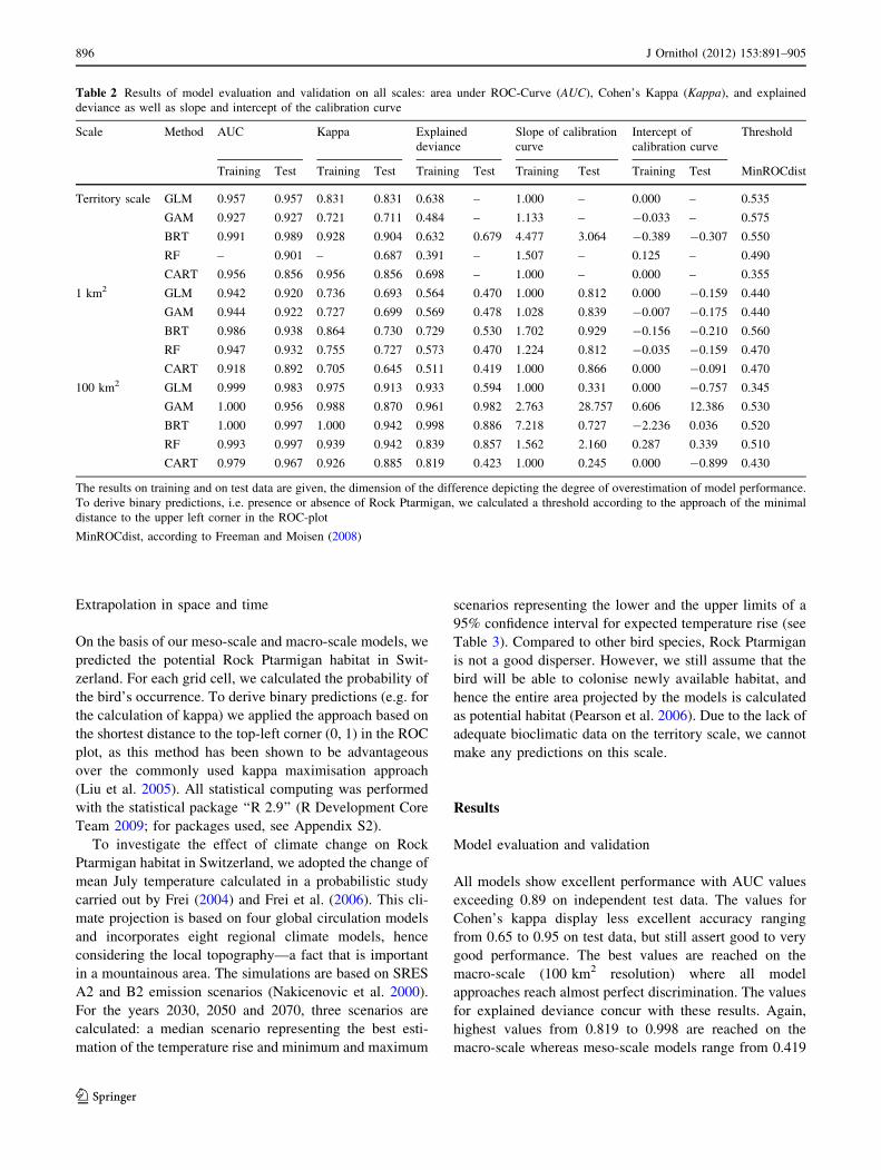
Model checking: evaluation and validation

In order to assess the goodness-of-fit of our models from

multiple perspectives, we calculated five different mea-

sures: the area under the receiver operating characteristic

curve (AUC; Fielding and Bell 1997), Cohen’s kappa sta-

tistic of similarity (j; Cohen 1960), the explained deviance,

slope and intercept of the calibration curve (cf. Reineking

and Schroder 2006). AUC and j both assess the discrimi-

natory power of the models. AUC values range from 0.5

(same predictive power as the null model) to 1 (denoting

perfect discrimination). According to Hosmer and Leme-

show (2000), an AUC value exceeding 0.9 reflects an

outstanding discrimination. For j (ranging from 0 to 1),

Monserud and Leemans (1992) propose a threshold of

j[ 0.85 for excellent discrimination. The explained

deviance measures the lack of fit of the model. It is cal-

culated as the quotient of the residual deviance and the

deviance of the null model subtracted from 1. Hence values

for models performing better than the null model range

from 0 to 1 with 1 depicting the best model. Slope and

intercept of the calibration curve investigate the degree of

overfitting of the model. Optimally calibrated models

exhibit a calibration curve with intercept 0 and slope 1

(Reineking and Schroder 2006; Table 2).

In order to gain reliable estimates of model perfor-

mance, models were tested on independent data (Araujo

et al. 2005). Hence, all models on the country-wide scales

were calibrated on training data representing 70% of the

original dataset; the remaining 30% served as test data.

Subsequently, all five measures (AUC, j, explained devi-

ance, slope and intercept of calibration curve) were cal-

culated on both datasets. The comparison of results on test

and training data reveals any over-confidence of model

performance.

A common problem working with spatial data in sta-

tistical modelling approaches is spatial autocorrelation.

This violates the model assumption of independency of

observations and may result in a misleading interpretation

of ecological relationships (e.g. Kuhn 2007; Lichstein et al.

2002). Therefore, models were checked for residual spatial

autocorrelation by calculating a global Moran’s I and

correlograms (Dormann et al. 2007).

Table 1 continued

Predictor variable Unit Median ptarmigan = 1 Median ptarmigan = 0

Snow bed vegetation Cover in % 0.5 0

Ericaceous dwarf shrubs Cover in % 0.05 0

Topography

Range of altitude within grid cell m 458.5 351.5

Profile curvature [1] -0.01 0.01

Slope Degree 12.46 10.27

Aspect (sine transformed) [1] -0.07 0.04

Aspect (cosine transformed) [1] 0.11 -0.21

Aspect (beers transformed) [1] 1.05 0.92

Distance to nearest ski lift m 3,162.28 3,000

For each predictor, estimates of the median are given for absence and presence of ptarmigan separately. On the meso-scale and macro-scale, the

following predictor variables had to be eliminated due to high multicollinearity (|qs| [ 0.7) with mean July temperature: degree days, annual

mean temperature, arable crop including vineyards, vegetation free areas, built-up areas, deciduous forest without shrub layer but with rich herbal

or dwarf shrub layer, minimal altitude in grid cell, median altitude in grid cell, maximum altitude in grid cell; with yearly precipitation:

precipitation January; with water budget July: precipitation July. Moreover, on the macro-scale only, range of altitude within grid cell had to be

removed because of multicollinearity with mean July temperature

J Ornithol (2012) 153:891–905 895

123

Extrapolation in space and time

On the basis of our meso-scale and macro-scale models, we

predicted the potential Rock Ptarmigan habitat in Swit-

zerland. For each grid cell, we calculated the probability of

the bird’s occurrence. To derive binary predictions (e.g. for

the calculation of kappa) we applied the approach based on

the shortest distance to the top-left corner (0, 1) in the ROC

plot, as this method has been shown to be advantageous

over the commonly used kappa maximisation approach

(Liu et al. 2005). All statistical computing was performed

with the statistical package ‘‘R 2.9’’ (R Development Core

Team 2009; for packages used, see Appendix S2).

To investigate the effect of climate change on Rock

Ptarmigan habitat in Switzerland, we adopted the change of

mean July temperature calculated in a probabilistic study

carried out by Frei (2004) and Frei et al. (2006). This cli-

mate projection is based on four global circulation models

and incorporates eight regional climate models, hence

considering the local topography—a fact that is important

in a mountainous area. The simulations are based on SRES

A2 and B2 emission scenarios (Nakicenovic et al. 2000).

For the years 2030, 2050 and 2070, three scenarios are

calculated: a median scenario representing the best esti-

mation of the temperature rise and minimum and maximum

scenarios representing the lower and the upper limits of a

95% confidence interval for expected temperature rise (see

Table 3). Compared to other bird species, Rock Ptarmigan

is not a good disperser. However, we still assume that the

bird will be able to colonise newly available habitat, and

hence the entire area projected by the models is calculated

as potential habitat (Pearson et al. 2006). Due to the lack of

adequate bioclimatic data on the territory scale, we cannot

make any predictions on this scale.

Results

Model evaluation and validation

All models show excellent performance with AUC values

exceeding 0.89 on independent test data. The values for

Cohen’s kappa display less excellent accuracy ranging

from 0.65 to 0.95 on test data, but still assert good to very

good performance. The best values are reached on the

macro-scale (100 km2 resolution) where all model

approaches reach almost perfect discrimination. The values

for explained deviance concur with these results. Again,

highest values from 0.819 to 0.998 are reached on the

macro-scale whereas meso-scale models range from 0.419

Table 2 Results of model evaluation and validation on all scales: area under ROC-Curve (AUC), Cohen’s Kappa (Kappa), and explained

deviance as well as slope and intercept of the calibration curve

Scale Method AUC Kappa Explained

deviance

Slope of calibration

curve

Intercept of

calibration curve

Threshold

Training Test Training Test Training Test Training Test Training Test MinROCdist

Territory scale GLM 0.957 0.957 0.831 0.831 0.638 – 1.000 – 0.000 – 0.535

GAM 0.927 0.927 0.721 0.711 0.484 – 1.133 – -0.033 – 0.575

BRT 0.991 0.989 0.928 0.904 0.632 0.679 4.477 3.064 -0.389 -0.307 0.550

RF – 0.901 – 0.687 0.391 – 1.507 – 0.125 – 0.490

CART 0.956 0.856 0.956 0.856 0.698 – 1.000 – 0.000 – 0.355

1 km2 GLM 0.942 0.920 0.736 0.693 0.564 0.470 1.000 0.812 0.000 -0.159 0.440

GAM 0.944 0.922 0.727 0.699 0.569 0.478 1.028 0.839 -0.007 -0.175 0.440

BRT 0.986 0.938 0.864 0.730 0.729 0.530 1.702 0.929 -0.156 -0.210 0.560

RF 0.947 0.932 0.755 0.727 0.573 0.470 1.224 0.812 -0.035 -0.159 0.470

CART 0.918 0.892 0.705 0.645 0.511 0.419 1.000 0.866 0.000 -0.091 0.470

100 km2 GLM 0.999 0.983 0.975 0.913 0.933 0.594 1.000 0.331 0.000 -0.757 0.345

GAM 1.000 0.956 0.988 0.870 0.961 0.982 2.763 28.757 0.606 12.386 0.530

BRT 1.000 0.997 1.000 0.942 0.998 0.886 7.218 0.727 -2.236 0.036 0.520

RF 0.993 0.997 0.939 0.942 0.839 0.857 1.562 2.160 0.287 0.339 0.510

CART 0.979 0.967 0.926 0.885 0.819 0.423 1.000 0.245 0.000 -0.899 0.430

The results on training and on test data are given, the dimension of the difference depicting the degree of overestimation of model performance.

To derive binary predictions, i.e. presence or absence of Rock Ptarmigan, we calculated a threshold according to the approach of the minimal

distance to the upper left corner in the ROC-plot

MinROCdist, according to Freeman and Moisen (2008)

896 J Ornithol (2012) 153:891–905

123

Table 3 Variable importance for the five different model approaches on the three scales (a) territory scale, (b) meso-scale (1 km2) and

(c) macro-scale (100 km2)

Predictor variable Model approach (criterion of predictor importance)

BRT RF GLM GAM CART

Rel. influence Out-of-bag T-effect (%) Drop contribution Primary split

(a) Territory scale

Simpson diversity index (vascular plants) 15.8 14.7 – – 1st split

Vegetation-free area 11.6 18.6 27.6 32 –

Aspect (cosine transformed) 9.6 – 10.2 – –

Depth of soil 8.0 12.3 – – 2nd split

Distance to ski fields 7.3 9.5 – – 4th split

Vaccinium uliginosum 6.8 9.1 12.8 – –

Vertical structure elements 6.2 8.2 19.1 – –

Vegetation height 6.2 8.5 – – 3rd split

Variability of topography 5.7 9.8 23.1 – –

Altitude 4.3 – – – 2nd split

Salix herbacea – 9.4 – – –

Herbal layer (cover) – 11.5 – 18.3 –

Juniperus communis (cover) – – 7.2 – –

Model approach (criterion of predictor importance)

BRT RF GLM GAM CART

Rel. influence %IncMSE T-effect (%) Drop contrib. Primary split

(b) Meso-scale (1 km2)

Snow bed vegetation 29.8 39.5 – – 1st split

Mean July temperature 26.0 48.7 29.5 101.7 2nd split

Uncultivated land 6.6 39.2 17.3 43.6 3rd split

Forest cover 6.1 42.3 22.9 40.1 2nd split

Profile curvature 4.1 33.2 10.0 56.1 –

Range of altitude within grid cell 3.8 26.6 – – –

Alp pasture 2.5 22.3 – – –

Low or sparse vegetation 2.3 28.9 – – –

Precipitation year 2.0 – – – –

Radiation July 1.9 – – – –

Streams – 20.0 – – –

Poor or no vegetation cover – 30.2 16.8 26.5 –

Water budget July – – – – 4th split

Ericaceous dwarf shrubs – – 3.5 – –

(c) Macro-scale (100 km2)

Mean July temperature 65.19 48.78 34.73 10.22 1st, 2nd and 3rd split

Ericaceous dwarf shrubs 15.30 27.32 12.20 12.40 2nd split

Water budget July 3.36 18.52 5.49 34.66 3rd split

Cloud cover July 3.06 18.28 – – –

Low or sparse vegetation 2.66 21.48 – – –

Precipitation July 2.10 5.74 – –

Dwarf and low shrubs 1.96 19.87 18.79 – –

Forest cover 1.71 – – –

Coniferous forest with rich herbal layer, no shrubs 1.63 14.44 – 10.22 –

Pond weed 0.83 – – –

Alp pasture – 13.97 11.64 25.07 –

Perennial plants (50–150 cm) – 16.01 – 28.83 –

J Ornithol (2012) 153:891–905 897

123

to 0.530 and on the territory scale from 0.391 to 0.698.

BRT generally exhibits the highest explained deviance.

The measures of model calibration, slope and intercept of

calibration curve, however, show a significant departure

from the ideal curve in BRT, whereas this is not the case

within the majority of the other modelling approaches

(Table 2). We detected a positive spatial autocorrelation in

the raw data, which was greatly reduced in the model

residuals. Adding an autocovariate reduced this to a non-

significant level (except for BRT, Appendix S3).

Generally, model predictions made by these different

approaches show a high correlation with the Spearman

rank correlation coefficient (qs) ranging between 0.887 and

0.990 (1 km2) and 0.868 and 0.943 (100 km2). The greatest

similarities occur among GLM and GAM; BRT and RF are

also closely correlated. Even though qs indicates great

coincidence among approaches, a scatter plot matrix and

the predicted geographical distribution reveal that for a few

individual grid cells the predictions diverge dramatically

(see Appendix S4 for scatter plot matrix and Appendix S5

for maps on spatial distribution of predicted potential

habitat by the different modelling approaches).

Habitat requirements of Rock Ptarmigan

The modelling approaches applied provide varying quan-

tifications of variable importance (Table 3). However, it is

possible to derive a general picture: a few predictor vari-

ables show good explanatory power throughout all model

approaches and even across scales.

Bioclimate

The most powerful variable on the meso-scale and macro-

scale is mean July temperature which is considered in all

models—contributing up to two-thirds of the explained

deviance in BRT. Response curves are hump-shaped at the

resolution of 1 km2 indicating that intermediate ranges of

temperature suit best. On the macro-scale, there is a purely

negative relationship between mean July temperature and

Rock Ptarmigan incidence. Surprisingly, further biocli-

matic variables do not seem to have a high impact on the

meso-scale. However, on the macro-scale, they gain

importance: The predictors annual precipitation, water

budget July and cloud cover July contribute clearly to the

distribution patterns of Rock Ptarmigan. Generally speak-

ing, regions receiving higher amounts of precipitation

represent more suitable habitats.

Vegetation

All modelling approaches single out low-growing vegeta-

tion types as adequate for Rock Ptarmigan, as well as areas

with sparse vegetation cover. In particular, snow bed

vegetation ranks among the variables with the highest

influence on the meso-scale, thus reflecting food avail-

ability. On the macro-scale, however, this variable had to

be discarded due to multicollinearity with mean July

temperature and hence is not present in these models. On

the territory scale, a diverse composition of dwarf shrubs

with vegetation-free patches resembles suitable habitat in

contrast to areas covered with a dense herbal layer, the

neighbourhood to downhill ski runs or higher vegetation

including small trees. Accordingly, large-scale models

clearly elucidate a negative relationship between forests

and Rock Ptarmigan habitat. However, a certain percentage

per grid cell appears to be tolerable, presumably where

trees are limited to the lower part of the grid cell.

Topography

On the meso-scale and macro-scale, primary topographic

attributes do not serve as good predictors with the excep-

tion of profile curvature on the meso-scale indicating ridges

Table 3 continued

Model approach (criterion of predictor importance)

BRT RF GLM GAM CART

Rel. influence %IncMSE T-effect (%) Drop contrib. Primary split

Coniferous forest with rich shrub layer – 23.27 – 34.35 –

Coniferous forest with sparse undergrowth – – – 34.88 –

Streams – – 11.41 – –

High shrubs – – – 8.90 –

The ten most important variables are displayed for ensemble forecasting techniques (RF and BRT), and for GLM, GAM and CART, the variables

composing the final model are shown. Note that different measures of variable importance apply: for BRT, relative influence calculated via

permutation test; for RF, difference between the Out-of-bag error of each tree and after permutation (Out-of-bag); for GLM, total contributing

effect derived via hierarchical partitioning (T-effect); for GAM, increase in deviance for model without variable (drop contribution); and for

CART, simply the primary splits are given

898 J Ornithol (2012) 153:891–905

123

as suitable habitat. In contrast, data on topography acquired

during field sampling explain a great part of the bird’s

preferences on the territory level. Here, the heterogeneity

and richness in geomorphologic features as well as vertical

structure elements depict suitable habitat as do northwest-

to northeast-facing slopes (see Table 3).

Potential habitat in Switzerland today and tomorrow

Figure 1 and Appendix S5 display the predicted geographical

distributions of potential Rock Ptarmigan habitat for recent

conditions in Switzerland according to the five modelling

approaches BRT, GLM, GAM, RF and CART. Furthermore,

its potential distribution for the year 2070 is shown based on

the scenario assuming an intermediate rise in mean July

temperature. Here, the maps indicate that former suitable

habitats at the northern and southern flanks of the Alps will

become increasingly unsuitable and that suitable habitat is

concentrated in the higher mountain regions in the central

Alps. Furthermore, highly suitable habitats with occurrence

probabilities exceeding 0.9 will fade.

The tendency of this development (i.e. shrinking of

potential habitat and forcing it uphill), is consistent

throughout all model approaches and at both grain sizes.

The intensity, however, varies strongly and ranges from a

reduction of 15% (CART) to more than two-thirds (GLM,

GAM, and BRT) in the maximum scenario 2070 (see

Table 3).

The rise in mean July temperature does not only affect

the extent of potential habitat but also the altitudinal range.

We predict a maximum upward shift ranging from 68 m

(CART) to 480 m (GLM) on the meso-scale and between

108 m (GAM) and 316 m (CART) on the macro-scale by

the year 2070. This represents a median upward shift of

21.2–46.5 m/�C on the meso-scale and of 5.2–44.4 m/�C

on the macro-scale.

Discussion

Evaluation, validation and uncertainties

of the multi-model approach

Our outlined model framework has proven to be successful

in modelling the current potential distribution of Rock

Ptarmigan and in identifying key habitat requirements

controlling the species’ distribution patterns. Performance

criteria show very good results on independent test data

proving a low degree of model overfitting (Table 2).

Generally speaking, the uncertainty in species distribu-

tion models can be divided into two parts: first, the algo-

rithmic error arising from data quality, variable selection

and applied modelling approach (Dormann et al. 2008);

and second, the biotic error that represents failures in

capturing all processes governing the species’ distribution

(of special concern are dispersal abilities, biotic interac-

tions, non-equilibrium situations; cf. Hampe 2004; Pearson

and Dawson 2003). It is noted that in our study not all

possible sources of biotic errors could be accounted for,

even though the study is based on high quality data. The

incorporation of many of the above-mentioned processes

still poses a great challenge to today’s species distribution

modelling (Zurell et al. 2009, 2011).

One of the most frequent sources of algorithmic pre-

diction error is the reliance on a single statistical model

(Pearson et al. 2006). The implementation of a multiple

model approach such as employed in this study leads to a

range of possible responses of Rock Ptarmigan to rising

temperatures—at a first glance. Although the five model-

ling techniques differ strongly regarding the modelling

procedure—i.e. selecting a single minimum adequate

model (GLM, GAM and CART) versus ensemble fore-

casting (BRT and RF), parametric versus semi-parametric

versus non-parametric approaches—the models are overall

in broad agreement. This is true in regards to habitat

requirements and with respect to the prediction of future

potential habitat. While climate change predictions vary in

magnitude, all models predict the same tendency: a sig-

nificant loss of suitable habitat and a shift to higher alti-

tudes (Table 4; Fig. 1; and Appendix S6). Similarly, the

characterisation of current Rock Ptarmigan habitat differs

slightly among these approaches. However, most predictors

with outstanding explanatory power in one model also

prove to be decisive in the other approaches (Table 3).

Rock Ptarmigan’s habitat requirements:

a matter of scale

In the following, we will examine the predicted suitable

habitat on the different spatial scales based on the results

for variable importance (Table 3). For an herbivorous

species such as Rock Ptarmigan one would expect vege-

tation types to be pivotal habitat determinants. However,

many studies state that the major drivers of species ranges

are climatic variables. For example, it is argued that land

cover plays a minor role as it can be widely explained

through climate (cf. Thuiller et al. 2004). This is certainly

true for continental-wide scales frequently used in most

macro-ecological studies. Our results demonstrate that

bioclimatic predictors gain explanatory power at the

coarser resolution. However, our results also coincide with

the findings of recent studies carried out by Pearson et al.

(2004), Luoto et al. (2007), von dem Bussche et al. (2008)

and Virkkala et al. (2010) asserting that bioclimatic pre-

dictors are large-scale determinants, amended by land

cover variables at finer resolutions.

J Ornithol (2012) 153:891–905 899

123

Mean July temperature is the dominant predictor in all

countrywide models. However, partial dependence plots

show a different correlation with Rock Ptarmigan inci-

dence: a linear, negative correlation on the macro-scale

and hump-shaped response curve on the meso-scale. This

does not reflect a differing mechanism of habitat selec-

tion. It can be explained by the fact that extreme values

disappear when grid cells are aggregated to a coarser

resolution, thus elucidating the need for analysis on fine

scales in order to avoid misleading interpretations of

results. The hump-shaped response curve on the meso-

scale confirms the observations by Marti and Bossert

(1985) indicating the rather narrow climatic niche of

Rock Ptarmigan. The countrywide scales indicate that

Rock Ptarmigan is confined to regions with mean July

temperatures below 10–12�C (slightly higher at the

100 km2 resolution). On the territory scale, bioclimatic

data as such is not available. However, there are proxies

that can explain the climatic constraints of Rock Ptar-

migan on this scale. For example, altitude can be

regarded as a substitute for temperature to a certain

extent (altitude and mean July temperature show a cor-

relation coefficient of qs \ -0.9 on the meso-scale and

macro-scale data). On the territory scale, altitude has

limited predictive power ranking amongst the least

influential variables. Here, climatic limitations of Rock

Ptarmigan are instead reflected in the preference of a

topography offering adequate and diverse micro-climatic

conditions. Models single out a preference for locations

with northeast- to northwest-facing slopes and habitats

with a large variation in topography and geomorphologic

features. In these locations, birds can adapt to seasonal

and short-term weather fluctuations by taking advantage

of differences in micro-site-specific climate. In fact,

local variation in climate can be much larger than

regional variation (Austin and van Niel 2011). Interpo-

lated climate surfaces commonly used in large-scale

modelling are at present not capable to integrate micro-

site-specific variations to sufficient detail and therefore

the gradient length of bioclimatic predictors is restricted

to large grain sizes. Rorison et al. (1986) for instance

recorded differences of up 12�C in maximum air tem-

peratures between north- and south-facing slopes during

the month of April.

This in turn explains the great explanatory power of

topographic variables on the territory scale where adequate

Fig. 1 Potential Rock

Ptarmigan (Lagopus mutahelvetica) habitat in Switzerland

at current conditions (a, c) and

for the intermediate scenarios

2070 (b, d) according to BRT at

the two spatial scales (a, b grain

size = 1 km2, c, d grain

size = 100 km2). If P(Rock

Ptarmigan) [ PMinROCdist grid

cells are assumed as suitable (cf.

Table 2); grid cells with

occurrence probabilities

exceeding 0.9 are considered as

highly suitable. See Appendix

S6 for maps based on the

remaining four model

approaches

900 J Ornithol (2012) 153:891–905

123

bioclimatic data is not available. On large scales, however,

the variables describing the topographic heterogeneity

simply lose their justification. Hence, apart from two

topographic attributes on the meso-scale, no topographic

variables were of importance for the countrywide

modelling.

Rock Ptarmigan is a bird species with a patchy distri-

bution and thus the extent of potential habitat is easily

overestimated by large-scale models. The true extent

however, can be highlighted by results of small-scale

analysis. Large-scale models, for instance, suggest Alp

pastures as suitable habitats, but the territory level analysis

shows that sites covered by a dense herbal layer are not

suitable as Rock Ptarmigan habitat. Hence, Alp pastures

seem to rather indicate a certain altitudinal range or the

neighbourhood of suitable patches within the grid cell.

Similarly, macro-scale models suggest grid cells containing

a forest cover of up to approx. 30% are still suitable habitat.

The territory-scale analysis, however, shows that the

occupied habitat lies well above the timberline and trees

are hardly tolerated within Rock Ptarmigan habitat. The

bird even avoids vegetation exceeding dwarf shrubs in

height, which is shown in univariate analysis on the terri-

tory scale (data not shown). This is also indicated by

vegetation-related predictor variables in large-scale models

and supported by observations from a ridge at the Aletsch

glacier. There, small Pinus cembra trees colonised an area

previously used by Rock Ptarmigan. Now, this area is

regularly used as a mating territory by Black Grouse

(Tetrao tetrix) instead (Bossert 1995; Marti et al., in

preparation).

The examples discussed above show that predictions

made on the territory scale can differ dramatically from

those delivered by the meso-scale and macro-scale mod-

elling. Figure 2 illustrates this subgrid variability. It shows

that, for the area of a single grid cell of 1 km2, the territory

model predicts suitable habitat patches as well as unsuit-

able patches in close vicinity, emphasising the spatial

heterogeneity of habitat suitability.

In conclusion, a multi-scale approach is a suitable tool

to approach scale-related problems. It contributes several

important insights which otherwise would be blurred by

scale-dependent effects. First, this approach shows the

changing importance of predictor variables across scales,

i.e. bioclimatic variables as large-scale determinants and a

crucial dependence of Rock Ptarmigan on topographic

features on the territory scale (which in turn can be related

to temperature tolerance of the bird). Downscaling,

therefore, would require consideration of information

about topography and vertical structure of habitat patches.

Second, it elucidates that observed patterns may be

strongly scale-dependent (e.g. a hump-shaped relationship

on one scale versus a steadily increasing one on the other).

These patterns do not necessarily depict a different habitat

selection process but may be solely explained by the way

data were gathered. Third, the assessment on multiple

scales allows the identifying of the true extent of suitable

habitat. According to performance criteria, all macro-

scale models reach nearly perfect results (Table 2).

However, this apparent gain of performance is accompa-

nied by a loss of quality of predictions: all macro-scale

models largely overestimate the area of suitable habitat

(Table 4; Fig. 1). This is especially the case if the species

under study relies on patchily distributed habitat and

inhabits steep terrain as do Rock Ptarmigan (Rahbek

2005; Popy et al. 2010). It clearly demonstrates how

invaluable small-scale atlas data can be to accurately

model the species distribution and its range shifts. The

territory analysis in turn reveals which habitat features

actually form the suitable area within the grid cell pre-

dicted as potential habitat on the meso-scale and visualise

sub-grid variability.

Response to climate change

Our study indicates that climate—especially summer

temperatures—is a main driving factor for Rock Ptarmi-

gan’s distribution in Switzerland. It is seen as a striking

model result that Rock Ptarmigan appeared to be confined

to regions with mean July temperatures below 10–12�C

(slightly higher in macro-scale models). The idea of a

strongly temperature-constrained dispersal of Rock Ptar-

migan is supported by the newly postulated ‘heat dissipa-

tion theory’ (Speakman and Krol 2010). This theory

suggests that endothermic animals are limited by the ability

to dissipate body heat rather than by the competition for a

limited energy supply. Hence, Rock Ptarmigan are

restricted to areas with rather low temperatures in order to

avoid hyperthermia despite the availability of adequate

food supply in warmer regions.

The climate change scenarios reflect this matter. Small

temperature changes during the breeding season will force

the species to higher altitudes. However, the calculated

upward shift in average over all models of 39.1 m/�C at

the meso-scale and 20.4 m/�C at the macro-scale is much

smaller than one would expect presuming a purely tem-

perature-driven distribution (a shift of ca. 160 m/�C;

Hughes 2000). Here, our modelling results coincide with

the empirical study of Popy et al. (2010) who detected a

shift in elevation of bird species in the Italian Alps of

29.4 m/C�. The results are also backed by findings of

Randin et al. (2009) as well as Luoto and Heikkinen

(2008) who stated that environmental heterogeneity may

significantly buffer the impact of climate change on spe-

cies distribution. In our study, the territory-scale analysis

elucidates the crucial dependence of Rock Ptarmigan on a

J Ornithol (2012) 153:891–905 901

123

diverse topography offering diverse microclimatic

conditions.

The shift of habitat from the current distributional range

to higher mountain regions indicates the presence of

potentially suitable habitat offering adequate conditions in

terms of vegetation and topography. Interestingly, in the

strongest scenario in BRT, RF and CART, the shift in

elevation is lower than in scenarios with a lesser

temperature rise, thus suggesting that there are no more

reserves of suitable habitat beyond a certain altitude.

Additionally, in some areas, dispersal to higher altitudes

will be simply restricted by the altitude of the mountain

ranges. Similarly, Virkkala et al. (2008) predict a drastic

reduction of Rock Ptarmigan habitat in northern Scandi-

navia. Here, the Arctic Ocean forms the northern barrier of

dispersal for Rock Ptarmigan.

Table 4 Development of potential Rock Ptarmigan habitat in Swit-

zerland applying scenarios for the rise of mean July temperature in

Switzerland according to minimal, median and maximal scenarios

represent the lower limit, the best estimation and the upper limit of a

95% confidence interval of temperature predictions for the years

2030, 2050 and 2070; habitat is estimated as suitable if P(Rock

Ptarmigan) [ PMinRocdist (cf. Table 2)

Model Current 2030 2050 2070

Min Median Max Min Median Max Min Median Max

D July temperature [?�C] 0 0.6 1.45 2.6 1.4 2.75 4.9 1.9 3.9 7.1

Decrease within scenarios (%)

Potential habitat (km2)

1 km2 resolution

BRT 9,450 -7.4 -16.7 -16.7 -7.1 -18.4 -45.4 -10.5 -31.2 -68.5

RF 9,955 -4.8 -8.9 -8.9 -4.6 -9.5 -15.3 -6.3 -12.8 -21.2

GLM 10,355 -1.5 -5.2 -13.5 -4.9 -15 -44 -7.7 -28.4 -81.8

GAM 10,216 -1.7 -5.2 -12.5 -5 -13.7 -39.7 -7.8 -26.3 -76.7

CART 10,699 -6.9 -11 -11 -6.7 -11.5 -14.1 -8.6 -13.5 -15.4

Median 10,216 -4.8 -8.9 -12.5 -5 -13.7 -39.7 -7.8 -26.3 -68.5

100 km2 resolution

BRT 241 -1.7 -3.7 -6.6 -3.7 -7.1 -21.2 -4.1 -14.5 -34.9

RF 240 -2.5 -3.8 -6.7 -4.2 -7.5 -15.4 -5.4 -12.1 -20.4

GLM 247 -4 -6.5 -10.5 -6.5 -10.5 -22.7 -8.5 -17.4 -39.3

GAM 234 -0.9 -2.1 -2.1 -1.7 -2.1 -10.3 -3.4 -5.6 -15.4

CART 240 -4.2 -9.6 -17.5 -9.6 -18.3 -31.3 -14.2 -22.9 -48.8

Median 240 -2.5 -3.8 -6.7 -4.2 -7.5 -21.2 -5.4 -14.5 -34.9

Upward shift within scenarios compared to current state (m)

Median of altitudinal distribution (m)

1 km2 resolution

BRT 2,319 56 100 100 54 108 149 73 145 17

RF 2,315 33 56 56 31 58 73 42 71 55

GLM 2,332 28 66 119 63 128 267 84 195 480

GAM 2,331 30 67 119 65 127 249 87 191 391

CART 2,360 35 55 55 34 57 70 44 68 63

Median 2,331 33 66 100 54 108 149 73 145 63

100 km2 resolution

BRT 1,601 12 17 24 17 34 189 18 122 247

RF 1,607 8 13 28 14 42 147 19 99 171

GLM 1,588 25 31 56 31 56 189 37 131 255

GAM 1,615 3 8 8 6 8 57 11 30 108

CART 1,607 14 56 151 56 156 235 116 171 316

Median 1,607 12 17 28 17 42 189 19 122 247

902 J Ornithol (2012) 153:891–905

123

Thus, the predicted changes in climate will have a

severe effect on Rock Ptarmigan distribution. A significant

distributional shift will be induced by changes below the

internationally agreed target of 2�C to which global

warming may be restricted within the twenty-first century

(IPCC 2007). If the temperature rise exceeds 4�C, potential

Rock Ptarmigan habitat will decrease drastically, between

one-quarter and two-thirds in the strongest scenario of

2070. Since we presume static conditions for all other

habitat determining factors besides climate, we have to

expect a more drastic development. Theurillat and Guisan

(2001) forecast a reduction by 63% in area of the alpine

layer for a ‘‘plus 3.3�C scenario’’.

Moreover, changing biotic interactions, shifting vegeta-

tion composition and transient dynamics will play important

roles (Zurell et al. 2009). For example, studies investigating

shifts of vegetational belts predict a certain time lag due to

the longevity of alpine shrubs and soil-forming processes

(Bolliger et al. 2000; Neilson et al. 2005). Last but not least,

the loss of habitat connectivity due to the displacement of

the species to mountain tops far apart from each other will

also contribute. Therefore, it should be noted that the sce-

narios presented in this study provide a conservative

approach to defining the lower limit of decrease of potential

habitat for Rock Ptarmigan. Linking the above-mentioned

processes to habitat distribution modelling will provide a

helpful tool for conservationists as they will need to adapt

their strategies to a dynamic environment.

Acknowledgments This study has been partly funded by the Ger-

man Academic Foreign Exchange Service (DAAD) and the Heinrich

Boll Foundation. Furthermore, we owe a big thank you to all col-

laborators who contributed to complete the Swiss breeding bird atlas

and to the reviewers who helped to improve the quality of the

manuscript.

References

Ackerly D, Loarie SR, Cornwell WK, Weiss SB, Hamilton H,

Branciforte R, Kraft NJB (2010) The geography of climate

change: implications for conservation biogeography. Divers

Distrib 16:476–487

Araujo MB, New M (2007) Ensemble forecasting of species

distributions. Trends Ecol Evol 22:42–47

Araujo M, Pearson RG, Thuiller W, Erhard M (2005) Validation of

species—climate impact models under climate change. Glob

Change Biol 11:1504–1513

Austin MP, Van Niel KP (2011) Improving species distribution

models for climate change studies: variable selection and scale.

J Biogeogr 38:1–8

Bolliger J, Kienast F, Zimmermann NE (2000) Risks of global

warming on montane and subalpine forests of Switzerland—a

modeling case study. Reg Environ Change 1(3–4):99–111

Bossert A (1995) Bestandsentwicklung und Habitatnutzung des

Alpenschneehuhns Lagopus mutus im Aletschgebiet (Schweizer

Alpen). Ornithol Beob 92(3):307–314

Brambilla M, Rubolini D, Guidali F (2006) Factors affecting breeding

habitat selection in a cliff-nesting peregrine Falco peregrinuspopulation. J Ornithol 147:428–435

Breiman L (2001) Random forests. Machine Learning 45:5–32

Cohen J (1960) A coefficient of agreement for nominal scales. Educ

Psychol Measur 20:37–46

Dormann CF, McPherson JM, Araujo MB, Bivand R, Bolliger J, Carl G,

Davis R, Hirzel A, Jetz W, Kissling WD, Kuhn I, Ohlemuller R,

Peres-Neto PR, Reineking B, Schroder B, Schurr FM, Wilson R

(2007) Methods to account for spatial autocorrelation in the analysis

of species distributional data: a review. Ecography 30:609–628

Dormann CF, Purschke O, Garcıa-Marquez J, Lautenbach S, Schroder

B (2008) Components of uncertainty in species distribution

analysis: a case study of the great grey shrike. Ecology

89(12):3371–3386

Dormann CF, Elith J, Bacher S, Buchmann C, Carl G, Carre G,

Garcia Marquez JR, Gruber B, Lafourcade B, Leitao PJ,

Munkemuller T, McClean C, Osborne P, Reineking B, Schroder

B, Skidmore A, Zurell D, Lautenbach S (2012) Collinearity: a

review of methods to deal with it and a simulation study

evaluating their performance. Ecography (in press)

Elith J, Graham CH, Anderson RP, Dudık M, Ferrier S, Guisan A,

Hijmans RJ, Huettmann F, Leathwick JR, Lehmann A, Li J,

Lohmann LG, Loiselle BA, Manion G, Moritz C, Nakamura M,

Nakazawa Y, Overton JM, Peterson AT, Phillips SJ, Richardson

K, Scachetti-Pereira R, Schapire RE, Soberon J, Williams S,

Wisz MS, Zimmermann NE (2006) Novel methods improve

prediction of species’ distributions from occurrence data.

Ecography 29:129–151

Elith J, Leathwick JR, Hastie T (2008) A working guide to boosted

regression trees. J Anim Ecol 77:802–813

Fasel M, Zbinden N (1983) Kausalanalyse zum Verlauf der sudlichen

Arealgrenze des Alpenschneehuhns Lagopus mutus im Tessin.

Ornithol Beob 80:231–246

Favaron M, Scherini GC, Preatoni D, Tos G, Wauters LA (2006)

Spacing behaviour and habitat use of rock ptarmigan (Lagopusmutus) at low density in the Italian Alps. J Ornithol 147:618–628

Fig. 2 Example for subgrid variability from Pizo Era ranges in

southern Switzerland in the Canton Ticino. Predicted Rock Ptarmigan

habitat by the meso-scale model (BRT, 1 9 1 km2 grid cells) and the

predictions of the territory model (BRT, dots). Red denotes suitable

habitat whereas green displays unsuitable habitat. Inset shows

location of Pizo Era ranges in Switzerland

J Ornithol (2012) 153:891–905 903

123

Fielding AH, Bell JF (1997) A review of methods for the assessment

of prediction errors in conservation presence-absence models.

Environ Conserv 24(1):38–49

Freeman EA, Moisen G (2008) Presenceabsence: an R package for

presence absence analysis. J Stat Softw 23:1–31

Frei C (2004) Die Klimazukunft der Schweiz—eine probabilistische

Projektion. In: Die Schweiz im Jahre 2050. OcCC, Bern

Frei C, Scholl R, Fukutome S, Schmidli J, Vidale PL (2006) Future

change of precipitation extremes in Europe: an intercomparison

of scenarios from regional climate models. J Geophys Res

Friedman JH (2002) Stochastic gradient boosting. Comput Stat Data

Anal 38:367–378

Glutz von Blotzheim UN, Bauer KM, Bezzel E (1973) Handbuch der

Vogel Mitteleuropas, vol 5: Galliformes und Gruiformes.

Akademische, Frankfurt a. M.

Graf RF, Bollmann K, Suter W, Bugmann H (2005) The importance

of spatial scale in habitat models: capercaillie in the Swiss Alps.

Landsc Ecol 20:703–717

Graham MH (2003) Confronting multicollinearity in ecological

multiple regression. Ecology 84:2809–2915

Guisan A, Zimmermann NE (2000) Predictive habitat distribution

models in ecology. Ecol Model 135(2–3):147–186

Hampe A (2004) Bioclimate envelope models: what they detect and

what they hide. Glob Ecol Biogeogr 13(5):469–471

Hegg O, Beguin C, Zoller H (1993) Atlas schutzwurdiger Vegeta-

tionstypen der Schweiz. Bundesamt fur Umwelt, Wald und

Landschaft, Bern

Hosmer DW, Lemeshow S (2000) Applied logistic regression. Wiley

series in probability and statistics, 2nd edn. Wiley, New York

Hughes L (2000) Biological consequences of global warming: is the

signal already apparent? Trends Ecol Evol 15:56–61

Huntley B, Collingham YC, Green RE, Hilton GM, Rahbek C, Willis

SG (2006) Potential impacts of climatic change upon geograph-

ical distributions of birds. Ibis 148:8–28

IPCC (2007) Fourth assessment report intergovernmental panel on

climate change. http://www.ipcc.ch/ipccreports/ar4-wg1.htm

Keller V, Gerber A, Schmid H, Volet B, Zbinden N (2010) Rote Liste

Brutvogel. Gefahrdete Arten der Schweiz, Stand 2010. Bunde-

samt fur Umwelt, Bern, und S chweizerische Vogelwarte,

Sempach. Umwelt-Vollzug Nr. 1019

Kuhn I (2007) Incorporating spatial autocorrelation may invert

observed patterns. Divers Distrib 13:66–69

Leathwick JR, Elith J, Francis MP, Hastie T, Taylor P (2006)

Variation in demersal fish species richness in the oceans

surrounding New Zealand: an analysis using boosted regression

trees. Mar Ecol Prog Ser 321:267–281

Lichstein JW, Simons TR, Shriner SA, Franzreb KE (2002) Spatial

autocorrelation and autoregressive models in ecology. Ecol

Monogr 72(3):445–463

Liu C, Berry PM, Dawson TP, Pearson RG (2005) Selecting

thresholds of occurrence in the prediction of species distribu-

tions. Ecography 28:385–393

Luoto M, Heikkinen RK (2008) Disregarding topographical hetero-

geneity biases species turnover assessments based on bioclimatic

models. Glob Change Biol 14:483–494

Luoto M, Virkkala R, Heikkinen RK (2007) The role of land cover in

bioclimatic models depends on spatial resolution. Glob Ecol

Biogeogr 16:34–42

Marti C, Bossert A (1985) Beobachtungen zur Sommerkativitat und

Brutbiologie des Alpenschneehuhns Lagopus mutus im Ale-

tschgebiet (Wallis). Ornithol Beob 82:153–168

Monserud RA, Leemans R (1992) Comparing global vegetation maps

with kappa statistic. Ecol Model 62:275–293

Nakicenovic N, Alcamo J, Davis G, de Vries B, Fenhann J, Gaffin S,

Gregory K, Grubler A, Yong Jung T, Kram T, Lebre La Rovere

E, Michaelis L, Mori S, Morita T, Pepper W, Pitcher H, Price L,

Riahi K, Roehrl A, Rogner H-H, Sankovski A, Schlesinger M,

Shukla P, Smith S, Swart R, van Rooijen S, Victor N, Dadi Z

(2000) Special report on emission scenarios. A special report of

working group III for the Integovernmental Panel on Climate

Change. Cambridge University Press, Cambridge

Neilson RP, Pitelka LF, Solomon AM, Nathan R, Midgley GF,

Fragoso JMV, Lischke H, Thompson K (2005) Forecasting

regional to global plant migration in response to climate change.

Bioscience 55:749–759

Oppel S, Schaefer HM, Schmidt V, Schroder B (2004) Habitat

selection by the pale-headed brush-finch, Atlapetes pallidiceps,

in southern Ecuador: implications for conservation. Biol Conserv118(1):33–40

Pearson RG, Dawson TP (2003) Predicting the impacts of climate

change on the distribution of species: are bioclimate envelope

models useful? Glob Ecol Biogeogr 12(5):361–372

Pearson RG, Dawson TP, Liu C (2004) Modelling species distribu-

tions in Britain: a hierarchical integration of climate and land-

cover data. Ecography 27(3):285–298

Pearson RG, Thuiller W, Araujo MB, Martinez-Meyer E, Brotons L,

Mcclean C, Miles L, Segurado P, Dawson TP, Lees DC (2006)

Model-based uncertainty in species range prediction. J Biogeogr

33:1704–1711

Popy S, Bordignon L, Prodon R (2010) A weak upward elevational

shift in the distributions of breeding birds in the Italian Alps.

J Biogeogr 37:57–67

Prasad A, Iverson LR, Liaw A (2006) Newer classification and

regression tree techniques: bagging and random forests for

ecological prediction. Ecosystems 9:181–199

R Development Core Team (2009) R: a language and environment for

statistical computing. R Foundation for Statistical Computing,

Vienna, Austria

Rahbek C (2005) The role of spatial scale and the perception of large-

scale species-richness patterns. Ecol Lett 8(2):224–239

Randin C, Engler R, Normand S, Zappa M, Zimmermann NE,

Pearman PB, Vittoz P, Thuiller W, Guisan A (2009) Climate

change and plant distribution: local models predict high-eleva-

tion persistence. Glob Change Biol 15(6):1557–1569

Reineking B, Schroder B (2006) Constrain to perform: regularization

of habitat models. Ecol Model 193:675–690

Rorison IH, Gupta PL, Hunt R (1986) Local climate, topography

and plant growth in Lathkill Dale NNR. II. Growth and

nutrient uptake within a single season. Plant Cell Environ

9:57–64

Schmid H, Luder R, Naef-Daenzer B, Graf R, Zbinden N (1998)

Schweizer Brutvogelatlas. Verbreitung der Brutvogel in der

Schweiz und im Furstentum Liechtenstein 1993–1996. Schwei-

zerische Vogelwarte, Sempach

Speakman JR, Krol E (2010) Maximal heat dissipation capacity and

hyperthermia risk: neglected key factors in the ecology of

endotherms. J Anim Ecol 79:726–746

Tanneberger F, Flade M, Preiksa Z, Schroder B (2010) Habitat

selection of the globally threatened Aquatic Warbler at the

western margin of the breeding range: implications for manage-

ment. Ibis 152:347–358

Theurillat J-P, Guisan A (2001) Potential impact of climate change on

vegetation in the European Alps: a review. Clim Change

50:77–109

Thomas CD, Lennon JJ (1999) Birds extend their ranges northwards.

Nature 399:213

Thompson CM, McGarigal K (2002) The influence of research scale

on bald eagle habitat selection along the lower hudson river,

New York (USA). Landsc Ecol 17(6):569–586

Thuiller W, Araujo MB, Lavorel S (2004) Do we need land-cover

data to model species distributions in europe? J Biogeogr

31(3):353–362

904 J Ornithol (2012) 153:891–905

123

Virkkala R, Heikkinen RK, Leikola N, Luoto M (2008) Projected

large-scale range reductions of northern-boreal land bird species

due to climate change. Biol Conserv 141:1343–1353

Virkkala R, Marmion M, Heikkinen RK, Thuiller W, Luoto M (2010)

Predicting range shifts of northern bird species: influence of

modelling technique and topography. Acta Oecol 36:269–281

von dem Bussche J, Spaar R, Schmid H, Schroder B (2008)

Modelling the recent and potential future spatial distribution of

ring ouzel (Turdus torquatus) and blackbird (T. merula) in

Switzerland. J Ornithol 149:529–544

Wilson JP, Gallant JC (2000) Terrain analysis: principles and

applications. Wiley, New York

Zurell D, Jeltsch F, Dormann CF, Schroder B (2009) Static species

distribution models in dynamically changing systems: how good

can predictions really be? Ecography 32(5):733–774

Zurell D, Grimm V, Rossmanith E, Zbinden N, Zimmermann NE,

Schroder B (2011) Uncertainty in predictions of range dynamics:

Black Grouse climbing the Swiss Alps. Ecography (in press).

doi:10.1111/j.1600-0587.2011.07200.x

J Ornithol (2012) 153:891–905 905

123