Librnry l':n!!ona! Wetlands Research Center U. Fish ari d. \lI, 'ildl!fe Service 7C:: Cajundoma Bo ulevard L ::. f"yetle. La. 70506 Biological Services Program FWS/OBS-82/10.4 FEBRUARY 1982 HABITAT SUITABILITY INDEX MODELS: CREEK CHUB SK 36 1 . U5 4 n o. 82- 10. 4 and Wildlife Service Department of the Interior
Transcript
Librnryl':n!!ona! Wetlands Research CenterU. ~) . Fish arid. \lI,'ildl!fe Service7C:: Cajundoma BoulevardL::.f"yetle. La . 70506
The Biological Services Program was established within the U.S. Fis hand Wild life Service to supply scientific information and methodolog ies onkey environmental issues that impact fish and wi ldli fe reso urces and theirsupporting ecosystems. The mission of the program is as follows:
• To strengthen the Fish and Wi ldl i fe Service i n its role asa primary source of information on national f ish and wildlife resources, particularly in respect to environmentalimpact assessment.
• To gather, analyze, and present info rmation that wi ll aiddecisionmakers in the identification and re sol'ut ion ofproble ms associated with major changes in land and wateruse.
• To provide bet ter ecological informat ion and eval uat ionfor Department of the Interior development programs , suchas those relating to energy developme nt.
Informat i on developed by the Biol ogi cal Ser vices Program is i nt endedfor use in the planning and decis ionma ki ng process to prevent or mi nimizethe impact of development on f i sh and wi ldli fe. Research activ ities andtec hnical assistance services are based on an analysis of t he issues , adetermina tion of t he decisionmakers involved and the i r i nformati on needs,and an evaluat ion of the state of t he art to iden ti fy i nformation Hapsand to determine pr iorit ies. This is a st ra t egy t hat wi l l ensure t hatthe products produced and di sseminated are t ime ly and useful.
Proj ect s -have been initiated i n t he following areas: coal ext ract ionand convers ion ; power plants; geot hermal , mi neral and oil shal e developmen t; wat er reso urce analysis , i ncl udi ng stream alterations and west ernwater allocation ; coastal ecosystems and Outer Con tinent al Shelf devel opment ; and systems invento ry , inc l uding Na ti onal Wetl and Inventory,habitat classi f i cation and analysi s, and informat i on transfer .
The Biological Servi ces Program cons ists of the Off i ce of Bi ol ogi calSer vi ces in Washingt on. D.C ., wh i ch i s res po nsi ble for overal l planning andma nagement; Nat.io.nal Teams, whi ch provide the Program's cent ral scien tifi c Iand tec hnical expertise and arrange for contract i ng bi ol o9ica l servicesstudies with states, universities, consulting firms , and othe r s; Regiona lStaffs, who provide a link to problems at the operating leve l ; and staffs atcertain Fish and Wil dli fe Ser vice resear ch fa cili t i es , wh o conduct i n-houseresearch studi es.
HABITAT SUITABILITY INDEX MODELS: CREEK CHUB
by
Thomas E. McMahonHabitat Evaluation Procedures GroupWestern Energy and Land Use Team
U.S. Fish and Wildlife ServiceDrake Creekside Building One
2625 Redwing RoadFort Collins, Colorado 80526
Western Energy and Land Use TeamOffice of Biological Services
Fish and Wildlife ServiceU.S. Department of Interior
Washington, D.C. 20240
FWS/OBS-82/10.4February 1982
This report should be cited as:
McMahon, T. E. 1982. Habitat suitability index models: Creek chub. U.S.D.l.Fish and Wildlife Service. FWS/OBS-82/10.4 23 pp.
ii
PREFACE
The habitat use information and Habitat Suitability Index (HSI) modelspresented in this document are an aid for impact assessment and habitat management activities. Literature concerning a species' habitat requirements andpreferences is reviewed and then synthesized into HSI models, which are scaledto produce an index between 0 (unsuitable habitat) and 1 (optimal habitat).Assumptions used to transform habitat use information into these mathematicalmodels are noted, and guidelines for model application are described. Anymodels found in the literature which-may also be used to calculate an HSI arecited, and simplified HSI models, based on what the authors believe to be themost important habitat characteristics for this species, are presented.
Use of the models presented in this publication for impact assessmentrequires the setting of clear study objectives and may require modification ofthe models to meet those objectives. Methods for reducing model complexityand recommended measurement techniques for model variables are presented inAppendix A.
The HSI models presented herein are complex hypotheses of species-habitatrelationships, not statements of proven cause and effect relationships.Results of mode,-performance tests, when available, are referenced; however,models that have demonstrated reliability in specific situations may proveunreliable in others. For this reason, the FWS encourages model users toconvey comments and suggestions that may help us increase the utility andeffectiveness of this habitat-based approach to fish and wildlife planning.Please send comments to:
Habitat Evaluation Procedures GroupWestern Energy and Land Use TeamU.S. Fish and Wildlife Service2625 Redwing RoadFt. Collins, CO 80526
iii
CONTENTS
Page
PREFACE iiiACKNOWLEDGEMENTS vi
HABITAT USE INFORMATION 1Genera 1 1Age, Growth, and Food 1Reproduct i on 1Specific Habitat Requirements. 1
HABITAT SUITABILITY INDEX (HSI) MODELS 3Model Applicability............................................. 3Mode 1 Descri pt ion 4Suitability Index (SI) Graphs for
Model Variables............................................... 6Riverine Model 14Lacustrine Model 21Interpreting Model Outputs...................................... 21
ADDITIONAL HABITAT MODELS 21Mode 1 1 21
REFERENCES CITED 21
v
ACKNOWLEDGEMENTS
I wish to acknowledge the contributions of Jack Gee and Fred Copes whoprovided many helpful comments and suggestions on earlier manuscripts. JohnFrench provided a preliminary literature review. Word processing was providedby Dora Ibarra and Carolyn Gulzow. The cover of this document was illustratedby Jennifer Shoemaker.
vi
CREEK CHUB (Semotilus atromaculatus)
HABITAT USE INFORMATION
General
The creek chub is a widely-distributed cyprinid ranging from the RockyMountains to the Atlantic Coast and from the Gulf of Mexico to southernManitoba and Quebec (Scott and Crossman 1973). Within its range, it is one ofthe most characteristic and common fishes of small, clear streams (Trautman1957).
Age, Growth, and Food
Creek chubs mature at age II-Vat lengths of 10.0-20.0 cm (Hubbs andCooper 1936; Dinsmore 1962; Copes 1978); average life span is 5-7 years (Hubbsand Cooper 1936; Copes 1978). Creek chubs exhibit wide variation in size andgrowth over their range (Copes 1978).
Fry feed on terrestrial and aquatic insects (Barber and Minckley 1971;Moshenko and Gee 1973; Copes 1978) and amphipods (Copes 1978). Creek chubsconsume larger food items as they grow (Scott and Crossman 1973). Juvenilesand adults feed on terrestrial and aquatic insects, molluscs, and fish (Barberand Minckley 1971; Moshenko and Gee 1973; Copes 1978). Fish dominate thesummer diet of creek chubs> 8 cm (Barber and Minckley 1971; Moshenko and Gee1973). The flexible food habits of creek chubs may account, in part, fortheir wide geographical distribution (Scott and Crossman 1973).
Reproduction
Creek chubs spawn in spring (April-July) (Trautman 1957; Pflieger 1975;Copes 1978) as water temperatures approach 14° C (Hubbs and Cooper 1936; Copes1978). Spawning occurs in gravel nests constructed by the male in shallowareas just above and below riffles (Miller 1964; Pflieger 1975; Copes 1978).
Successful reproduction in creek chubs is adversely affected by watertemperatures < 11° C (Miller 1964; Moshenko and Gee 1973; Copes 1978), highturbidity and-Siltation (Miller 1964), and low flows (Paloumpis 1958).
Specific Habitat Requirements
Optimum habitat for creek chubs is small, clear, cool streams withmoderate to high gradients, gravel substrate, well-defined riffles, and poolswith abundant cover and abundant food (Trautman 1957; Moshenko and Gee 1973;Hocutt and Stauffer 1975). Small populations occasionally occur in ponds andlakes, but these are not preferred creek chub habitats (Eschmeyer and Clark1939; Trautman 1957).
Creek chubs are found in streams with gradients of 3 to 23 m/km with theirgreatest abundance in gradients of 7 to 13.4- m/km (Moshenko and Gee 1973;
Hocutt and Stauffer 1975). They are most abundant in small streams 0.5 to 7 min width (Hocutt and Stauffer 1975) and less than 1 m in average depth (Barberand Minckley 1971; Hocutt and Stauffer 1975). Streams greater than 12 m inwidth (Starrett 1950; Dinsmore 1962) and greater than 2 m in average depth(Minckley 1963; Powles et al. 1977) are considered marginal habitats.
Creek chubs are most abundant in clear water (Barber and Minckley 1971;Minckley 1963; Scott and Crossman 1973) but can tolerate higher turbidities ifareas of clean gravel substrate for spawning are present (Branson and Batch1972, 1974; Pfl i eger 1975). Creek chubs are found in moderate abundance inhighly turbid streams in North Dakota (Copes and Tubbs 1966).
Creek chubs appear to be more tolerant of acidic conditions than manyother species (Smith 1964). F. A. Copes (pers. comm., Mus. of Nat. Hist.,Univ. of Wisconsin, Stevens Point) has observed sustaining populations ofcreek chubs in streams with a pH as low as 5.4. However, a pH range of 6.0 to9.0 is probably optimum for survival and growth of creek chub populations(McKee and Wolf 1963; Minckley 1963).
Creek chubs are most abundant in streams wi th alternat i ng pools andriffle-run areas (Trautman 1957; Minckley 1963; Moshenko and Gee 1973). Weassume that stream sections with 40-60% pools are optimum for providing riffleareas for spawning habitat (Moshenko and Gee 1973) and pools for cover(Moshenko and Gee 1973; Copes 1978). Rubble substrate in riffles, abundantaquatic vegetation (Hynes 1970), and abundant streambank vegetation (Moshenkoand Gee 1973; Cummins 1974) are conditions associated with high production offood types consumed by creek chubs. Streambank vegetation in creek chubhabitats is also considered important for stream shading (for water temperaturecontrol) and bank stability (for erosion control) (Karr and Schlosser 1978).
Creek chubs are most numerous in deep pools and runs with abundant instream cover of cut-banks, roots, aquatic vegetation, brush, and large rocks(Trautman 1957; Copes 1978). It is assumed that at 1east 40% pool and runareas with suitable cover is optimum. Deep pools with abundant cover, freeaccess to larger, warmer streams within 5 km, or both, are important forover-wintering habitat (Trautman 1957; Paloumpis 1958; Copes 1978). Creekchubs are found over all types of substrate. Abundance appears to be correlated more with the amount of instream cover than with substrate type (Copesand Tubb 1966; Copes 1970, 1978, pers. comm.).
Adult. The upper incipient lethal temperature for adult creek chubs isnear 32° C; the lower lethal level is near 1.7° C (Brett 1944; Hart 1947).They can survive intermittent streamflow in isolated pools for short periodsin summer at temperatures of 28° C (Starrett 1950). Creek chubs grow in thetemperature range of 12-24° C, with the optimum temperature for growth near21° C (Miller 1964; Moshenko and Gee 1973).
Di sso 1ved oxygen data are not avail ab1e for adul ts. If oxygen requi rements are similar to those for other coolwater fishes, concentrations ~ 5 mg/lshould be sufficient for long-term growth and survival (Davis 1975). Creekchubs can survive for short periods in pools with 2.4 mg/l of dissolved oxygen(Starrett 1950). The creek chub is generally not found in lakes, ponds, orstreams which experience partial summer- or winter-kills (long-term D.O.deficiency) (Copes, pers. comm.). Adults generally occur in streams with an
2
average velocity of less than 60 cm/sec (Minckley 1963; Moshenko and Gee1973). They are most abundant in stream sections of deep runs and pools withsurface velocities ~ 30 cm/sec (Moshenko and Gee 1973).
Embryo. Eggs hatch in 10 days at 13° C (Washburn 1945). Embryos requireflowing water for adequate oxygen exchange. Embryo survival and productionare highest in gravel substrate in riffle-run areas with velocities of20-64 cm/sec (Ross 1976; Copes 1978); production is negligible in sand or silt(Washburn 1945; Trautman 1957). Washburn (1945) listed 0.04 m3/sec (1.25 cfs)as the minimum discharge necessary for successful reproduction. High survivaland production of creek chub embryos are associ ated wi th temperatures of15-20° C (Clark 1943; Moshenko and Gee 1973; Copes 1978) and dissolved oxygenlevels ~ 5 mg/l (Davis 1975).
Fry. Fry emerge from nests 20-30 days after spawning (Washburn 1945;Copes 1970; Moshenko and Gee 1973). After emergi ng from redds ,' fry are foundin shallow areas along the edges of pools with surface velocities < 10 cm/sec(Clark 1943; Minckley 1963; Copes 1978).
The di sso 1ved oxygen and temperature sui tabi 1ity cri teri a for fry areassumed to be similar to those for adults.
Juvenile. No specific information was found on habitat requirements ofjuveniles. We assume habitat requirements are similar to those of adults.
HABITAT SUITABILITY INDEX (HSI) MODELS
Model Applicability
Geographic area. The model provided is assumed to be applicable to anyriverine environment within the range of creek chubs. The standard of comparison for each individual variable suitability index is the optimum value ofthe vari ab1e that occurs anywhere wi thi n thi s range. It shoul d be noted,however, that specifying only one set of standards defining optimum habitatfor creek chubs is somewhat tenuous since it occurs in such a wide variety ofhabitats throughout its extensive range (Copes, pers. comm.). Availableinformation on habitat requirements of creek chubs is, however, insufficientat this time to specify more than one set of standards defining optimum conditions in various regions throughout its range.
Season. The model provides a rating for a riverine habitat based on itsabi 1i ty to support all 1i fe stages of creek chubs thro.ughout all seasons ofthe year.
Cover types. This mode l is applicable in riverine environments, asdescribed by Cowardin et al. (1979).
Minimum habitat area. Mjnimum habitat area is defined as the minimumarea of contiguous suitable habitat that is required for a species to live andreproduce. No attempt has been made to establish a minimum habitat sizenecessary for long-term survi va1 of creek chubs.
3
Verifi cat ion 1eve1. The acceptable output of thi s mode 1 is an indexbetween 0 and 1 which the author believes has a positive relationship tocarrying capacity of a habitat for creek chub populations. In order to verifythat the model output was acceptable, sample data sets (described later) weredeveloped for calculating HSI's from the model. These sample data sets andtheir relationship to model verification are discussed in greater detailfollowing the presentation of the model.
Model Description
The model consists of variables that have an impact on the growth,survival, distribution, abundance, or other measure of well-being of creekchubs, and hence can be expected to have an impact on the carrying capacity ofa habitat. Creek chub habitat quality is based primarily on their food,cover, water quality, and reproduction requirements, and the model consists ofvariables which are thought to be direct or indirect measures of the relativeability of a habitat to meet these requirements (Fig. 1). Variables thataffect habitat quality for creek chubs, but which do not easily fit into thesefour major components, are combi ned under the "other component" headi ng(Fig. 1).
Food component. Percent streambank (riparian) vegetation (V g ) is included
in the food component since streamside vegetation is habitat for terrestrialinsects, an important food source for creek chubs. Substrate type (V lO ) is
included for rating the food component because production potential of aquaticinsects (another important constituent in the diet of creek chubs) in a streamis related to amount and type of substrate.
Cover component. Percent pools (Vi) is included since pools are utilized
as cover by adults, juveniles, and fry. A pool class rating system (V 2 ) is
included because the depth of a pool affects its suitability for providingcover for creek chubs. Percent cover (V 3 ) is included in this component to
provide a measure of the amount of cover available within a stream. A measureof winter instream cover suitability (V 4 ) is included since creek chubs require
instream cover in pools or free access to larger, warmer streams to provideshelter during winter. A measure of velocities suitable for adults andjuveniles (V 1 3 ) and fry (ViS) are included in this component because velocity
can affect the quality of a habitat as resting cover.
Water quality component. Turbidity (V,) is included because abundance of
creek chubs is related to turbidity level. Measures of pH (V s ) , average water
temperature (Vii), and dissolved oxygen (V 1 2 ) are included in this component
since these water qual ity parameters have been shown to affect growth andsurvival of creek chubs. Any of these latter three variables are assumed tobecome overriding determinants of overall habitat suitability if the variablesapproach lethal levels.
Stream shade (V 1 9 ) is included in this component since the magnitude of
daily and seasonal temperature extremes that occur in a small stream areinversely related to the amount of stream shaded from the sun.
4
Habitat Variables Life Requisites
% streambank vegetation (V g )~ Food (C F)% substrate type (V 10)------------
Stream gradient (V s ) --
Average stream width (V,) Other (COT)
Average stream depth (V20)~
Wa te r qua1ity (CWQ) ------oJ HS I
% poo 1s (V 1)--------______
Pool class rating system (V2)% cover (V 3 ) -------------=::::~~
Winter instream cover suitability (V 4 )
Average current velocity (adult, juvenile)
Average current velocity (fry) (Vla)-----------~
Average water temperat~Dissolved oxygen (ViS) Reproduction (C R)Average current velocity (Vi')
% substrate type (V 17)
Turbi dity (V 7)
pH (Va)
Average water temperature (Vii)
Dissolved oxygen (V 12)% stream shade (V 19)
Figure 1. Tree diagram illustrating relationship of habitat variablesand life requisites in the creek chub model.
5
Reproduction component. Average water temperature (V 1 4 ) and dissolved
oxygen (VIS) are included since they affect survival and production of creek
chub embryos. A measure of velocity in riffle-run sections during spawning(VIi) is included because current velocity affects the water exchange rate in
creek chub redds. Substrate type (VI') in the same areas is included in this
component since reproductive success of creek chubs varies with type of spawning substrate available.
Other component. Stream gradient (V s ) , average stream width (Vi), and
average stream depth (V 2 0 ) are included in this component since the abundance
of creek chubs has been observed to vary with these three parameters.
Suitability Index (SI) Graphs for Model Variables
This section contains suitability index graphs for the 20 variablesdescribed above, and equations for combining the suitability index (S1) ofeach variable into a species HSI using the component approach. All variablespertain to a riverine (R) habitat.
Habitat
R
Variable
Percent pools duringaverage summer flow.
1.0
xQ) 0.8"'0c......e-, 0.6~
'r-
'r- 0.4..cn:l~'r-~ 0.2V)
0.0
a
Suitability Graph
50 100
- ~
- ~
~
- ~
R (V 2 ) Dominant (> 50%) poolclass rating during
1.0average summer flow.x 0.8Q)
"'0C......
~0.6
'r-
'r- 0.4..an:l~'r-~ 0.2V)
0.0
6A
%
B
Class
C
A) First-class pools (large and deep): Pool depth and size is sufficientto provide a low velocity resting area for numerous creek chubs. Morethan 30% of the pool bottom is obscured due to surface turbul ence,depth, or the presence of structures, e.g., logs, debris piles,boulders, or overhanging banks and vegetation.
B) Second-class pool (moderate size and depth): Pool depth and size ares~fficient to provide a low velocity resting area for some creek chubs.From 5 to 30% of the bottom is obscured due to surface turbul ence,depth, or the presence of structures. Typical second-class pools arelarge eddies behind boulders and low velocity, moderately deep areasbeneath overhanging banks and vegetation.
C) Third-class pool (small or shallow or both): Pool depth and sizeprovide a low velocity resting area for only a very few creek chubs.Cover, if present, is in the form of shade, surface turbulence, or verylimited structure. Typical third-class pools are wide, shallow poolsor small eddies behind boulders. Virtually the entire bottom of thepool is discernible.
R
R
(V 3 ) Percent cover during 1.0summer within poolsand runs. x 0.8QJ
"'C~.....>, 0.6
.j-J'r-r-'r- 0.4..ClItl-4-l'r-:::I 0.2V')
0.0
a 25 50(V .. ) Winter instream cover %suitability.
A) If access to larger,warmer streams is> 5 km from studyarea, then
B) If access is within 5 km,then
1/3V.. = (VI X V% x V3 ) + 0.2,or 1.0, whichever issmaller
highly embedded or 0.0compacted or if thesubstrate is anoxic( i .e. , H2S present). a 50 100
%
12
R (V 18) Velocity along edges 1.0of stream during average xsummer flow (Fry). Q)
"'0 0.8c......>, 0.6+J
'r-r--'r-..c 0.4ttl+J'r-:::::lVl 0.2
0.0
a 30 60
em/sec
R (V 19 ) Average percent of 1.0stream shaded between1000 and 1500 hours x
Q)
during midsummer. "'0 0.8c......>, 0.6+J'r-r-e-'r-
0.4..cttl+J'r-
:::::l0.2Vl
0.0
a 50 100
%
R (V 2 0 ) Average of maximum 1.0stream depths duringaverage summer flow. x
Q)"'0 0.8c......>,
0.6+J'r-r-e-'r-..c 0.4ttl+J
:::::lVl 0.2
0.0
a 2m
13
Riverine Model
This model utilizes the life requisite approach and consists of fivecomponents: Food, Cover, Water Quality, Reproduction, and Other.
C = ---=---F 2
Water Qual i ty (CWQ)
CWQ = (V 7 x VB X VII XVl 2 x VI9) 1/ 5
If VB' VII' or Vl 2 is ~ 0.4, then CWQ equals the lowest of the following:
VB' VII' V1 2 , or the above equation.
Reproduction (CR)
CR = (V 1 4 x VIS XVl 6 x VI72 )1/ 5
If Vl 4 or VIS is ~ 0.4, then CR equals the lowest of the following: V1 4 ,
VIS' or the above equation.
14
HSI determination
HSI = (C F x Cc x CWQ
x CR x COT) 1/ 5
If CC' CWQ' or CR is S 0.4, then the HSI equals the lowest of the
following: CC' CWQ' CR' or the above equation.
Sources of data and assumptions made in developing the suitability indicesare presented in Table 1.
Sample data sets used in calculating HSI's from the above model are givenin Table 2. The data sets are not actual field measurements, but the differentvariable values used in calculating the HSI's are thought to represent realistic conditions that could occur in creek chub riverine habitats. The HSI'scalculated from the data seem to reflect what carrying capacity trends wouldbe in riverine habitats with the listed characteristics. Thus, the modelmeets the acceptance goal of produci ng an index between 0 and 1 whi ch isthought to have a positive relationship to carrying capacity of a habitat forcreek chubs.
15
Table 1. Data sources and assumptions for creek chub suitability indices.
Variable and source
Trautman 1957Minckley 1963Moshenko and Gee 1973
Moshenko and Gee 1973Copes 1978
Trautman 1957Copes 1978
Trautman 1957Paloumpis 1958Copes 1978
Trautman 1957Moshenko and Gee 1973Hocutt and Stauffer 1975
Starrett 1950Dinsmore 1962Hocutt and Stauffer 1975
Minckley 1963Barber and Minckley 1971Branson and Batch 1972Scott and Crossman 1973Pfl i eger 1975
McKee and Wolf 1963Minckley 1963Smith 1964
Assumption
Streams with approximately equalamounts of pools and riffles willprovide optimum conditions formeeting the needs of creek chubsfor covert spawning habitat t andfood (aquatic insects).
Large and deep pools are most suitableas cover for creek chubs; shallowand or small pools are suboptimum.
The high abundance of creek chubs inareas with instream cover indicatesthat optimum conditions will occurin areas with high amounts of instreamcover.
Optimum conditions for winter coverare large t deep pools with abundantinstream cover or free access tolarger streams within 5 km.
Streams with gradients correspondingto those with high abundance of creekchubs are optimum.
Streams with widths corresponding tothose with high abundance of creekchubs are optimum.
Turbidity levels associated with highabundance of creek chubs are optimum.
The pH range that is associated withhigh abundance of creek chubs and thatis most suitable for survival andgrowth of freshwater fishes is optimum.
16
Table 1. (continued)
Variable and source Assumption
Vg Moshenko and Gee 1973Cummins 1974
Hynes 1970
The amount and type of streambankvegetation associated with highallochthonous input (terrestrialinsects) of food for creek chubs isoptimum. In terms of productionof terrestrial insects, shrubs>grasses-forbs > trees> bare ground.
The amount and type of substrate orthe amount of aquatic vegetationassociated with high production ofaquatic insects (used as food by creekchubs) is optimum.
Vll Brett 1944Hart 1947Starrett 1950Miller 1964Moshenko and Gee 1973
V12 Davis 1975
Minckley 1963Moshenko and Gee 1973
Clark 1943Moshenko and Gee 1973Copes 1978
Davis 1975
Moshenko and Gee 1973
Temperature levels associated withhighest growth are optimum. Levelsassociated with reduced survival andgrowth are suboptimum.
Levels associated with high survivaland growth of freshwater fish in generalare considered optimum for creek chubs.Levels where survival is poor areunsuitable.
Velocities where creek chub adults andjuveniles are most abundant are optimum.Velocities where creek chub adults andjuveniles are less abundant aresuboptimum.
Temperature levels associated withhigh survival and production areoptimum.
Levels associated with high survivalof embryos of coolwater fishes areconsidered to be optimum for creekchubs.
Velocities where survival and production of creek chub embryos are highestare optimum.
Minckley 1963Miller 1964Barber and Minckley 1971Hocutt and Stauffer 1975Powles et al. 1977
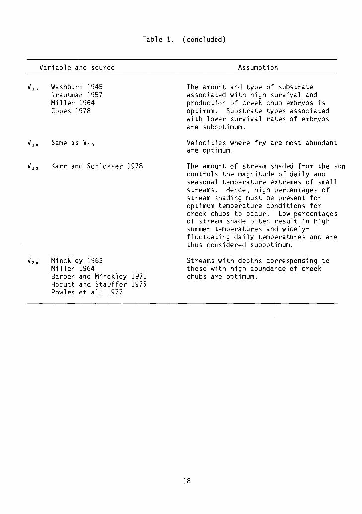
The amount and type of substrateassociated with high survival andproduction of creek chub embryos isoptimum. Substrate types associatedwith lower survival rates of embryosare suboptimum.
Velocities where fry are most abundantare optimum.
The amount of stream shaded from the suncontrols the magnitude of daily andseasonal temperature extremes of smallstreams. Hence, high percentages ofstream shading must be present foroptimum temperature conditions forcreek chubs to occur. Low percentagesof stream shade often result in highsummer temperatures and widelyfluctuating daily temperatures and arethus considered suboptimum.
Streams with depths corresponding tothose with high abundance of creekchubs are optimum.
18
Table 2. Sample data sets using riverine HS1 model.
Data set 1 Data set 2 Data set 3
Variable Data S1 Data S1 Data S1
% pools V1 60 1.0 75 0.5 90 0.1
Pool class V2 A 1.0 B 0.6 e 0.3
% cover V3 30 0.9 15 0.5 75 1.0
Winter cover V4 0.76 0.53 0.5
Gradient (m/km) V5 14.5 0.9 16.5 0.6 2 0.3
Width (m) V6 3 1.0 10 0.5 1.5 0.9
Turbidity (JTU) V7 25 1.0 90 0.5 105 0.3
pH Va 7.5 1.0 5.5 0.8 9.5 0.8
Streambank vegeta-tation index Vs 75 1.0 30 0.4 10 0.1
Substrate(for food prod.) VlO A 1.0 e 0.5 0 0.2
Temperature (Oe) - Vll 19 1.0 25 0.5 25 0.5A, J, F
D.O. (mg/l) - A,J,F V12 6 1.0 4 0.9 3 0.5
Velocity (em/sec) -A,J V13 20 1.0 10 1.0 2 0.5
Temperature (Oe) - E V14 15 1.0 20 1.0 23 0.5
D.O. (mg/l) - E V15 6 0.9 5 0.75 4 0.5
Velocity (em/sec) - V16 30 1.0 17 0.8 5 0.2E
Substrate index -spawning V17 55 0.8 45 0.6 35 0.4
Velocity (em/sec) - V18 5 1.0 2 1.0 < 1 1.0F
19
Table 2. (concluded)
Data set 1 Data set 2 Data set 3
Variable Data SI Data SI Data SI
% shade Vl9 80 1.0 45 0.7 15 0.3
Stream depth (m) V2 0 1.5 1.0 2.0 0.2 1.8 0.3
Component SI
CF = 1.00 0.45 0.15
Cc = 0.94 0.66 0.44
CWQ = 1. 00 0.66 0.45
CR = 0.90 0.74 0.38
COT = 0.97 0.43 0.50
HS1 = 0.96 0.57 0.38 1
lNote: HS1 equals CR' since CR ~ 0.4.
20
Lacustrine Model
Specific lacustrine suitability indices for creek chub were not developeddue to a lack of information on habitat requirements and limited use of lacustrine habitats by creek chubs. Small populations might occur if suitablespawning habitat near shoreline is present, i.e., gravel substrates with somecurrent (Scott and Crossman 1973).
Interpreting Model Outputs
The HSI for creek chubs as determined by one of the above models may notnecessarily represent the exact population level of creek chubs in the studyarea. This may be due to the fact that these models rely on habitat-basedfactors, and other factors may be operating that more significantly affect thepopulation level of creek chubs present in an area. If the HSI's calculatedfrom the models are a good representation of creek chub habitat quality, thenin riverine environments where creek chub population levels are due primarilyto habitat-based factors, the HSI should be positively correlated to thelong-term average population levels. However, this has not been tested. Theproper interpretation of the HSI is one of comparison. If two study areashave different HSI's, the one with the higher HSI should have the potential tosupport more creek chubs than the one with the lower HSI, given that the modelassumptions have not been violated.
ADDITIONAL HABITAT MODELS
Model 1
Optimum riverine habitat for creek chubs is characterized by the followingconditions, assuming water quality is adequate: small (~7 m wide); cool(summer temperatures 19-23° C)~ at least 40% gravel substrate; approximately50% pools:SO% riffles-runs; abundant (~ 40%) instream cover.
HSI = number of above criteria present5
REFERENCES CITED
Barber, W. E., and W. L. Minckley. 1971. Summer foods of the cyprinid fishSemotilus atromaculatus. Trans. Am. Fish. Soc. 100(2):283-289.
Baxter, G. T., and J. R. Simon. 1970. Wyoming fishes. Wyoming Game FishDept. Bull. 4. 168 pp.
Branson, B. A., and D. L. Batch. 1972. Effects of strip rm rn nq on smallstream fishes in east-central Kentucky. Proc. Biol. Soc. Wash.84(59):507-517.
21
Branson, B. A., and D. L. Batch. 1974. Additional observations on the effectsof strip mining on small-stream fishes in east-central Kentucky. Trans.Ky. Acad. Sci. 35(3-4):81-83.
Brett, J. R.fishes.49 pp.
1944. Some lethal temperature relations of Algonquin ParkUniv. Toronto Stud., Bio1. Ser. 52. Pub1. Onto Fish. Res. Lab.
Clark, C. F. 1943. Creek chub minnow propagation. Ohio Conserv. Bull.7(6):12-13.
Copes, F. A. 1970. Ecology of the native fishes of Sand Creek, Albany County,Wyoming. Ph.D. Thesis. Univ. Wyoming, Laramie. 281 pp.
Copes, F. A. 1978. Ecology of the creek chub. Univ. Wisc., Stevens Point,Mus. Nat. Hist., Rept. on Fauna and Flora of Wisc. No. 12. 21 pp.
Copes, F. A., and R. A. Tubbs. 1966. Fishes of the Red River Tributaries inNorth Dakota. Inst. for Eco1. Stud., Univ. N. Dakota No. 1. 25 pp.
Cowardin, L. M., V. Carter, F. C. Go1et, and E. T. LaRoe. 1979. Classification of wetlands and deepwater habitats of the United States. U.S. FishWild1. Serv., FWS/OBS-79/31. 103 pp.
Cummins, K. W. 1974. Structure and function of stream ecosystems. BioScience24:631-641.
Davis, J. C. 1975. Minimal dissolved oxygen requirements of aquatic lifewith emphasis on Canadian species: a review. J. Fish. Res. Board Can.32:2295-2332.
Dinsmore, J. J. 1962. Life history of the creek chub, with emphasis ongrowth. Proc. Iowa Acad. Sci. 69:296-301.
Eschmeyer, R. W., and D. H. Clark. 1939. Analysis of the populations of fishin the waters of the Mason Game Farm, Mason, Michigan. Ecology20(2):272-286.
Hart, J. S. 1947. Lethal temperature relations of certain fish of the Torontoregion. Trans. Royal Soc. Can. (Third Ser., Sec. V) 41 :57-71.
Hocutt, C. H., and J. R. Stauffer. 1975. Influence of gradient on the distribution of fishes in Conowingo Creek, Maryland and Pennsylvania.Chesapeake Sci. 16(1):143-147.
Hubbs, C. L., and G. P. Cooper. 1936. Minnows of Michigan. Cranbrook Inst.Sci. Bull. 8. 95 pp.
Hynes, H. B. N. 1970. The ecology of running waters. Univ. Toronto Press,Can. 555 pp.
Karr, J. R., and 1. J. Schlosser. 1978. Water resources and the land-waterinterface. Science 201:229-234.
22
McKee, J. E., and H. W. Wolf. 1963. Water quality criteria. State WaterQuality Control Board. Sacramento, Calif. Publ. 3A. 548 pp.
Miller, R. J. 1964. Behavior and ecology of some North American cyprinidfishes. Am. Midl. Nat. 72(2):313-357.
Minckley, W. E. 1963. The ecology of a spring stream, Doe Run, Meade County,Kentucky. Wil d1. Monogr. 11: 124 pp.
Moshenko, R. W., and J. H. Gee. 1973. Diet, time and place of spawning, andenvironments occupied by creek chub (Semotilus atromaculatus) in the MinkRiver, Manitoba. J. Fish Res. Board Can. 30(3):357-362.
Paloumpis, A. A. 1958. Responses of some minnows to flood and drought conditions in an intermittent stream. Iowa State Coll. J. Sci. 32(4):547-561.
Pfl i eger, W. L. 1975. The fi shes of Mi ssouri. Mi ssouri Dept. of Con serv.343 pp.
Powles, P. M., D. Parkes, and R. Reid. 1977. Growth, maturation, and apparentand absolute fecundity of creek chub, Semotilus atromaculatus (Mitchill),in the Kawartha Lakes region, Ontario. Can. J. Zool. 55(5):843-846.
Ross, M. R. 1976. Nest-entry behavior of female creek chubs (Semotilusatromaculatus) in different habitats. Copeia 1976(2):378-380.
Scott, W. B., and E. J. Crossman. 1973. Freshwater fi shes of Canada. Bull.Fish. Res. Board Can. 184. 966 pp.
Smith, M. A. 1964. Fish population. Pages B80-B83 in C. R. Colier, G. W.Whetstone, and J. J. Musser (eds.). Influences Of strip minning on thehydrologic environment of parts of Beaver Creek Basin, Kentucky,1955-1959. U.S. Geol. Sur. Prof. Pap. 427-B. 85 pp.
Starrett, W. C. 1950. Distribution of the fishes of Boone County, Iowa, withspecial reference to the minnows and darters. Am. Midl. Nat.43( 1) : 112-127.
Trautman, M. B. 1957. The fishes of Ohio. bhio State Univ. Press, Columbus.683 pp.
Washburn, G. N. 1945. Propagation of the creek chub in ponds with artificialraceways. Trans. Am. Fish. Soc. 75:336-350.
23
50272 "01
REPORT DOCUMENTATION 11. REPORT NO.1
2•
3. Rec:lplenrs Acc.._ No.
PAGE FWS/ORS-R?/lO.44. TItle and Subtitle 5. Repart Oate
Habitat Suitability Index Models: Creek chubFebruarv 1982
I.
7. Authorisl I. Performln, O,..ntzatlon Rept. No.
Thomas E. McMahon9. Performln, ·O,..nlzation Name and Addr... Habitat Evaluation Procedures Group 10. PnJject/Ta.Il/Wor!o: Unit No.
Western Energy and Land Use TeamU.S. Fish and Wildlife Service 11. Contrsct(C) or Grant(GI No.
Drake Creekside Building One (C)
2625 Redwing Road (GlFort Co 11 ins, Colorado 80526
12. Spansorin, O..anlzstlon Neme and Addres. Western Energy and Land Use Team 13. TYIM of Report & Period Covered
Office of Biological ServicesFish and Wildlife ServiceU.S. Department of Interior 14.
Washinqton. D.C. 2024015. Supplementary Note.
11. Abstract (Limit: 200 _rd.)
Literature describing the habitat preferences of the creek chub (Semotilus atromaculatus )is reviewed, and the relationships of habitat variables and life requisites in thecreek chub are illustrated.
This is one in a series of publications developed to provide informati.on on thehabitat requirements of selected fish and wildlife species. Numerous literaturesources have been consulted in an effort to consolidate scientific data on species-habitat relationships. These data have subsequently been synthesized into explicitHabitat Suitability Index (HSI) models. The models are based on suitability indicesindicating habitat preferences. Indices have been formulated for variables found toaffect the life cycle and survival of each species. Habitat Suitability (HSI) modelsare designed to provide information for use in impact assessment and habitat managementactivities. The HSI technique is a corollary to the U.S. Fish and Wildlife Service'sHabitat Evaluation Procedures.
17. Oocument Analysi. a. Oescriptors
Habitabil ityFishes
b. Identlfiers/OPen·Ended Term.
Creek chubSemitilus atromaculatusHabitat Suitability Index
~ U. S. GOVERNMENT PRINTING OFFICE 1982 - 578-126/188 Reg. 8
(S.. ANSI-z39.181 s•• 'nstruetions on Reve,.,. O"'ONAL FORM 272 (4-77)(Formerly NTI5-35)Oepartment of Commerce
•
••• ..__ ....J~.
' .'· 0 ,,-
Hawaiian Islands (>
-(:( Headq uarters . Division of BiologicalServices, Wasnington, DC
x Eastern Energy anO Land Use TeamLeetown , WV
* Nationa l Coastal Ecosystems TeamSli dell , LA
• Western Energy and Land Use TeamFt. Coll ins . CO
• Locat ions of Regional Off ices
REGION 1Regional DirectorU,S. Fish and Wildlife ServiceLloyd Five Hundred Building, Suite 1692500 N.E. Multnomah StreetPortland , Oregon 97232
REGION 4Regional DirectorU.S. Fish and Wildlife ServiceRichard B. Russell Building75 Spring Street , S.W.Atlanta, Georgia 30303
IJ- - - ----
6 1r-- - -~-
L, JI : - ~- --I I
1- - -'I Il,_I 2 ,,-~--
-_.J
REGION 2Regional DirectorU.S. Fish and Wildlife ServiceP.O. Box 1306Albuquerque, New Mexico 87 103
REGION 5Regional DirectorU.S. Fish and Wildlife ServiceOne Gateway Cente rNewton Corner, Massachusetts 02158
REGION 7Regional DirectorU.S. Fish and Wildlife ServicelOll E. Tudor RoadAnchorage, Alaska 99503
- ..~,.
REGION 3Regional DirectorU.S. Fish and WildlifeServiceFederal Building, Fort SnellingTwin Cities, Minnesota 551 J I
REGION 6Regional DirectorU.S. Fish and Wildli fe ServiceP.O. Box 25486Denver Federal CenterDenver, Colorado 8022 5
u.s.FISH ..WILDLIFE
f>ERVICE
DEPARTMENT OF THE INTERIOR hi?]u.s.FISH ANDWILDLIFESERVICE ~
"'-r rw T " "
As the Nat ion's pri ncipal conservation agency, the Department of the Interior has responsibility for most of our ,nationally owned public lands and natural resources . This includesfostering the wisest use of our land and water resources, protecting our fish and wildlife,preserving th & environmental and cultural values of our national parks and historical places,and providing for the enjoyment of life through outdoor recreation. The Department assesses our energy and mineral resources and works to assure that t heir development is inthe best interests of all our people. The Department also has a major respons ibility forAmerican Indian reservation communit ies and for people who live in island territories underU.S. adm inist ration.