Hadwiger’s conjecture and squares of chordal graphs

L. Sunil Chandran1∗, Davis Issac2 and Sanming Zhou3†

1 Indian Institute of Science, Bangalore -560012, India

sunil@csa.iisc.ernet.in

2 Max Planck Institute for Informatics, Saarland Informatics Campus, Germany

dissac@mpi-inf.mpg.de

3 School of Mathematics and Statistics, The University of Melbourne, Parkville, VIC 3010, Australia

sanming@unimelb.edu.au

Abstract

Hadwiger’s conjecture asserts that any graph contains a clique minor with order no lessthan the chromatic number of the graph. We prove that this well-known conjecture is truefor all graphs if and only if it is true for squares of split graphs. Since all split graphs arechordal, this implies that Hadwiger’s conjecture is true for all graphs if and only if it is truefor squares of chordal graphs. It is known that 2-trees are a class of chordal graphs. Wefurther prove that Hadwiger’s conjecture is true for squares of 2-trees. In fact, we provethe following stronger result: for any 2-tree T , its square T 2 has a clique minor of orderχ(T 2) for which each branch set is a path, where χ(T 2) is the chromatic number of T 2.As a corollary, we obtain that the same statement holds for squares of generalized 2-trees,and so Hadwiger’s conjecture is true for such squares, where a generalized 2-tree is a graphconstructed recursively by introducing a new vertex and making it adjacent to a singleexisting vertex or two adjacent existing vertices in each step, beginning with the completegraph of two vertices.

Key words: Hadwiger’s conjecture; minors; split graph; chordal graph; 2-tree; generalized2-tree; square of a graph

AMS subject classification: 05C15, 05C83

1 Introduction

A graph H is called a minor of a graph G if a graph isomorphic to H can be obtained from

a subgraph of G by contracting edges. An H-minor is a minor isomorphic to H, and a clique

minor is a Kt-minor for some positive integer t, where Kt is the complete graph of order t.

The Hadwiger number of G, denoted by η(G), is the largest integer t such that G contains a

Kt-minor. A graph is called H-minor free if it does not contain an H-minor.

In 1937, Wagner [15] proved that the Four Color Conjecture is equivalent to the following

statement: If a graph is K5-minor free, then it is 4-colorable. In 1943, Hadwiger [8] proposed

the following conjecture which is a far reaching generalization of the Four Color Theorem.

Conjecture 1.1. For any integer t ≥ 1, every Kt+1-minor free graph is t-colorable.

Hadwiger’s conjecture is well known to be a challenging problem. Bollobas, Catlin and Erdos

[4] describe it as “one of the deepest unsolved problems in graph theory”. Hadwiger himself [8]

∗Part of the work was done when this author was visiting Max Planck Institute for Informatics, Saarbruecken,Germany supported by Alexander von Humboldt Fellowship.†Research supported by ARC Discovery Project DP120101081.

1

arX

iv:1

603.

0320

5v4

[m

ath.

CO

] 1

1 N

ov 2

016

proved the conjecture for t = 3. (The conjecture is trivially true for t = 1, 2.) In view of Wagner’s

result [15], Hadwiger’s conjecture for t = 4 is equivalent to the Four Color Conjecture, the latter

being proved by Appel and Haken [1, 2] in 1977. In 1993, Robertson, Seymour and Thomas [14]

proved that Hadwiger’s conjecture is true for t = 5. The conjecture remains unsolved for t ≥ 6,

though for t = 6 Kawarabayashi and Toft [9] proved that any graph that is K7-minor free and

K4,4-minor free is 6-colorable.

Hadwiger’s conjecture has been proved for several classes of graphs, including line graphs [13],

proper circular arc graphs [3], quasi-line graphs [6], 3-arc graphs [16], complements of Kneser

graphs [17], and powers of cycles and their complements [10]. Since Hadwiger’s conjecture is

equivalent to the statement that η(G) ≥ χ(G) for any graph G, where χ(G) is the chromatic

number of G, there is also an extensive body of work on the Hadwiger number. See for example

[5] for a study of the Hadwiger number of the Cartesian product of two graphs and [7] for a

recent work on the Hadwiger number of graphs with small chordality.

It would be helpful if one could reduce Hadwiger’s conjecture for all graphs to some special

classes of graphs. In this paper we establish a result of this type. A graph is called a split graph

if its vertex set can be partitioned into an independent set and a clique. The square of a graph

G, denoted by G2, is the graph with the same vertex set as G such that two vertices are adjacent

if and only if the distance between them in G is equal to 1 or 2. The first main result in this

paper is as follows.

Theorem 1.2. Hadwiger’s conjecture is true for all graphs if and only if it is true for squares

of split graphs.

A graph is called a chordal graph if it contains no induced cycles of length at least 4. Since

split graphs form a subclass of the class of chordal graphs, Theorem 1.2 implies:

Corollary 1.3. Hadwiger’s conjecture is true for all graphs if and only if it is true for squares

of chordal graphs.

These results show that squares of chordal or split graphs capture the complexity of Had-

wiger’s conjecture, though they may not make the conjecture easier to prove.

In light of Corollary 1.3, it would be interesting to study Hadwiger’s conjecture for squares

of some subclasses of chordal graphs in the hope of getting new insights into the conjecture. As

a step towards this, we prove that Hadwiger’s conjecture is true for squares of 2-trees. It is well

known that chordal graphs are precisely those graphs that can be constructed by recursively

applying the following operation a finite number of times beginning with a clique: Choose a

clique in the current graph, introduce a new vertex, and make this new vertex adjacent to all

vertices in the chosen clique. If we begin with a k-clique and choose a k-clique at each step,

then the graph constructed this way is called a k-tree, where k is a fixed positive integer. The

second main result in this paper is as follows.

Theorem 1.4. Hadwiger’s conjecture is true for squares of 2-trees. Moreover, for any 2-tree

T , T 2 has a clique minor of order χ(T 2) for which all branch sets are paths.

A graph is called a generalized 2-tree if it can be obtained by allowing one to join a fresh

vertex to a clique of order 1 or 2 instead of exactly 2 in the above-mentioned construction of

2-trees. (This notion is different from the concept of a partial 2-tree which is defined as a

subgraph of a 2-tree.) The class of generalized 2-trees contains all 2-trees as a proper subclass.

The following corollary is implied by (and equivalent to) Theorem 1.4.

Corollary 1.5. Hadwiger’s conjecture is true for squares of generalized 2-trees. Moreover, for

any generalized 2-tree G, G2 has a clique minor of order χ(G2) for which all branch sets are

paths.

2

In general, in proving Hadwiger’s conjecture it is interesting to study the structure of the

branch sets forming a clique minor of order no less than the chromatic number. Theorem 1.4

and Corollary 1.5 provide this kind of information for squares of 2-trees and generalized 2-trees

respectively.

A quasi-line graph is a graph such that the neighborhood of every vertex can be partitioned

into two (not necessarily non-empty) cliques. We call a graph G a generalized quasi-line graph

if for any ∅ 6= S ⊆ V (G) there exists a vertex u ∈ S such that the set of neighbors of u in

S can be partitioned into two vertex-disjoint (not necessarily non-empty) cliques. It is evident

that quasi-line graphs are trivially generalized quasi-line graphs, but the converse is not true.

We observe that the square of any 2-tree is a generalized quasi-line graph but not necessarily

a quasi-line graph. Chudnovsky and Fradkin [6] proved that Hadwiger’s conjecture is true for

all quasi-line graphs. It would be interesting to investigate whether Hadwiger’s conjecture is

true for all generalized quasi-line graphs. Theorem 1.4 can be thought as a step towards this

direction: It shows that Hadwiger’s conjecture is true for a special class of generalized quasi-line

graphs that is not contained in the class of quasi-line graphs.

All graphs considered in the paper are finite, undirected and simple. As usual the vertex

and edge sets of a graph G are denoted by V (G) and E(G), respectively. If u and v are adjacent

in G, then uv denotes the edge joining them. As usual we use χ(G) and ω(G) to denote the

chromatic and clique numbers of G, respectively. A proper coloring of G using exactly χ(G)

colors is called an optimal coloring of G. A graph G is t-colorable if t ≥ χ(G).

An H-minor of a graph G can be thought as a family of t = |V (H)| vertex-disjoint connected

subgraphs G1, . . . , Gt of G such that the graph constructed in the following way is isomorphic

to H: Identify all vertices of each Gi to obtain a single vertex vi, and draw an edge between

vi and vj if and only if there exists at least one edge of G between V (Gi) and V (Gj). Each

subgraph Gi in the family is called a branch set of the minor H. This equivalent definition of a

minor will be used throughout the paper.

2 Proof of Theorem 1.2

It suffices to prove that if Hadwiger’s conjecture is true for squares of all split graphs then it is

also true for all graphs.

So we assume that Hadwiger’s conjecture is true for squares of split graphs. Let G be an

arbitrary graph with at least two vertices. Since deleting isolated vertices does not affect the

chromatic or Hadwiger number, without loss of generality we may assume that G has no isolated

vertices. Construct a split graph H from G as follows: For each vertex x of G, introduce a vertex

vx of H, and for each edge e of G, introduce a vertex ve of H, with the understanding that all

these vertices are pairwise distinct. Denote

S = {vx : x ∈ V (G)}, C = {ve : e ∈ E(G)}.

Construct H with vertex set V (H) = S∪C in such a way that no two vertices in S are adjacent,

any two vertices in C are adjacent, and vx ∈ S is adjacent to ve ∈ C if and only if x and e

are incident in G. Obviously, H is a split graph as its vertex set can be partitioned into the

independence set S and the clique C.

Claim 1: The subgraph of H2 induced by S is isomorphic to G.

In fact, for distinct x, y ∈ V (G), vx and vy are adjacent in H2 if and only if they have

a common neighbor in H. Clearly, this common neighbor has to be from C, say ve for some

e ∈ E(G), but this happens if and only if x and y are adjacent in G and e = xy. Therefore, vxand vy are adjacent in H2 if and only if x and y are adjacent in G. This proves Claim 1.

3

Claim 2: In H2 every vertex of S is adjacent to every vertex of C.

This follows from the fact that C is a clique of H and x is incident to at least one edge in G.

Claim 3: χ(H2) = χ(G) + |C|.In fact, by Claim 1 we may color the vertices of S with χ(G) colors by using an optimal

coloring of G (that is, choose an optimal coloring φ of G and assign the color φ(x) to vx for each

x ∈ V (G)). We then color the vertices of C with |C| other colors, one for each vertex of C. It is

evident that this is a proper coloring of H2 and hence χ(H2) ≤ χ(G) + |C|. On the other hand,

since C is a clique, it requires |C| distinct colors in any proper coloring of H2. Also, by Claim

2 none of these |C| colors can be assigned to any vertex of S in any proper coloring of H2, and

by Claim 1 the vertices of S needs at least χ(G) colors in any proper coloring of H2. Therefore,

χ(H2) ≥ χ(G) + |C| and Claim 3 is proved.

Claim 4: η(H2) = η(G) + |C|.To prove this claim, consider the branch sets of G that form a clique minor of G with order

η(G), and take the corresponding branch sets in the subgraph of H2 induced by S. Take each

vertex of C as a separate branch set. Clearly, these branch sets produce a clique minor of H2

with order η(G) + |C|. Hence η(H2) ≥ η(G) + |C|.To complete the proof of Claim 4, consider an arbitrary clique minor of H2, say, with branch

sets B1, B2, . . . , Bk. Define B′i = Bi if Bi∩C = ∅ (that is, Bi ⊆ S) and B′i = Bi∩C if Bi∩C 6= ∅.It can be verified that B′1, B

′2, . . . , B

′k also produce a clique minor of H2 with order k. Thus,

if k > η(G) + |C|, then there are more than η(G) branch sets among B′1, B′2, . . . , B

′k that are

contained in S. In view of Claim 1, this means that G has a clique minor of order strictly bigger

than η(G), contradicting the definition of η(G). Therefore, any clique minor of H2 must have

order at most η(G) + |C| and the proof of Claim 4 is complete.

Since we assume that Hadwiger’s conjecture is true for squares of split graphs, we have

η(H2) ≥ χ(H2). This together with Claims 3-4 implies η(G) ≥ χ(G); that is, Hadwiger’s

conjecture is true for G. This completes the proof of Theorem 1.2.

3 Proof of Theorem 1.4

3.1 Prelude

By the definition of a k-tree given in the previous section, a 2-tree is a graph that can be

recursively constructed by applying the following operation a finite number of times beginning

with K2: Pick an edge e = uv in the current graph, introduce a new vertex w, and add edges uw

and vw to the graph. We say that e is processed in this step of the construction. We also say that

w is a vertex-child of e, each of uw and vw is an edge-child of e, e is the parent of each of w, uw

and vw, and uw and vw are siblings of each other. An edge e2 is said to be an edge-descendant

of an edge e1, if either e2 = e1, or recursively, the parent of e2 is an edge-descendant of e1. A

vertex v is said to be a vertex-descendant of an edge e if v is a vertex-child of an edge-descendant

of e.

An edge e may be processed in more than one step. If necessary, we can change the order

of edge-processing so that e is processed in consecutive steps but the same 2-tree is obtained.

So without loss of generality we may assume that for each edge e all the steps in which e is

processed occur consecutively.

We now define a level for each edge and each vertex as follows. Initially, the level of the

first edge and its end-vertices is defined to be 0. Inductively, any vertex-child or edge-child of

an edge with level k is said to have level k + 1. Observe that two edges that are siblings of

each other have the same level. If there exists a pair of edges e, f with levels i, j respectively

4

such that i < j and the batch of consecutive steps where e is processed is immediately after the

batch of consecutive steps where f is processed, then we can move the batch of steps where e is

processed to the position immediately before the processing of f without changing the structure

of the 2-tree. We repeat this procedure until no such a pair of edges exists. So without loss of

generality we may assume that a breadth-first ordering is used when processing edges, that is,

edges of level i are processed before edges of level j whenever i < j.

To prove Theorem 1.4, we will prove η(T 2) ≥ χ(T 2) for any 2-tree T . In the simplest case

where χ(T 2) = 2, this inequality is true as T 2 has at least one edge and so contains a K2-minor.

Moreover, in this case both branch sets of this K2-minor are singletons (and so are paths of

length 0).

In what follows T is an arbitrary 2-tree with χ(T 2) ≥ 3. Denote by Ti the 2-tree obtained

after the ith step in the construction of T as described above. Then there is a unique positive

integer ` such that χ(T 2) = χ(T 2` ) = χ(T 2

`−1) + 1. Define

G = T`.

We will prove that η(G2) ≥ χ(G2) and G2 has a clique minor of order χ(G2) for which each

branch set is a path. Once this is achieved, we then have η(T 2) ≥ η(G2) ≥ χ(G2) = χ(T 2) and

T 2 contains a clique minor of order χ(T 2) whose branch sets are paths, as required to complete

the proof of Theorem 1.4.

Given X ⊆ V (G), define

N(X) = {v ∈ V (G) \X : v is adjacent in G to at least one vertex in X}.

Define

N [X] = N(X) ∪X, N2[X] = N [N [X]], N2(X) = N2[X] \X.

In particular, for x ∈ V (G), we write N(x), N [x], N2(x), N2[x] in place of N({x}), N [{x}],N2({x}), N2[{x}], respectively.

Denote by `max the maximum level of any edge of G. Then the maximum level of any vertex

in G is also `max. Observe that the level of the last edge processed is `max − 1, and none of

the edges with level `max has been processed at the completion of the `-th step, due to the

breadth-first ordering of processing edges. Obviously, `max ≤ `.If lmax = 0 or 1, then G2 is a complete graph and so χ(G2) = ω(G2) = η(G2). Moreover, G2

contains a clique minor of order χ(G2) for which each branch set is a path of length 0. Hence

the result is true when lmax = 0 or 1.

We assume lmax ≥ 2 in the rest of the proof. We will prove a series of lemmas that will be

used in the proof of Theorem 1.4. See Figure 1 for relations among some of these lemmas.

3.2 Pivot coloring, pivot vertex and its proximity

Lemma 3.1. There exist an optimal coloring µ of G2 and a vertex p of G at level lmax such

that p is the only vertex with color µ(p).

Proof. Let v be the vertex introduced in step `. Then v has level lmax. By the definition of

G = T`, there exists a proper coloring of T 2`−1 using χ(G2) − 1 colors. Extend this coloring to

G2 by assigning a new color to v. This extended coloring φ is an optimal coloring of G2 under

which v is the only vertex with color φ(v).

Note that, apart from the pair (φ, v) in the proof above, there may be other pairs (µ, p) with

the property in Lemma 3.1.

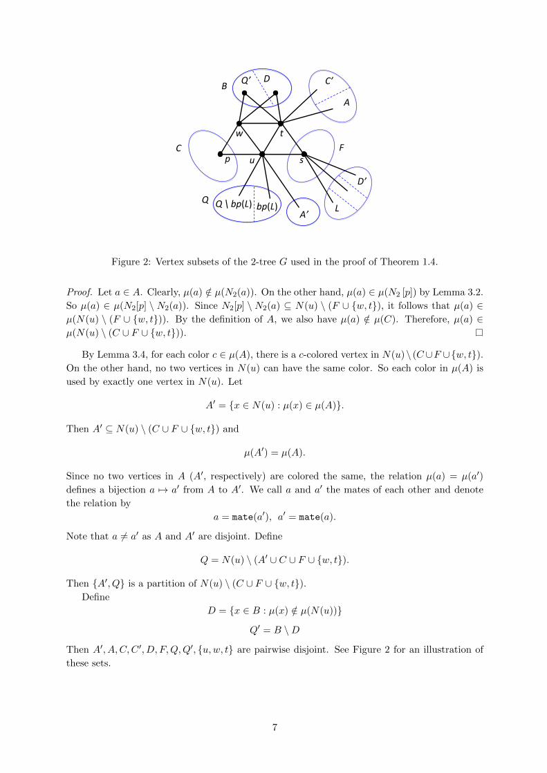
In the remaining part of the paper, we will use the following notation and terminology (see

Figure 2 for an illustration):

5

3.6  

3.7   3.9  

3.11  

3.12   3.15   3.16  

3.13   3.17   3.18  

3.14   3.20   3.19  Finale  

3.21  

3.23            3.22  3.2  

Proof  of  Theorem  1.4  

Defini<on  of  s  

3.10  

3.8  

Figure 1: Lemmas to be proved and their relations.

• µ, p: an optimal coloring of G2 and a vertex of G, respectively, as given in Lemma 3.1; we

fix a pair (µ, p) such that the minimum level of the vertices in N(p) is as large as possible;

we call this particular µ the pivot coloring and this particular p the pivot vertex ;

• uw: the parent of p;

• t: the vertex such that w is a child of ut, so that the level of ut is `max − 2, and uw and

wt are siblings with level `max − 1 (the existence of t is ensured by the fact `max ≥ 2);

• B: the set of vertex-children of wt;

• C: the set of vertex-children of uw;

• µ(X) = {µ(x) : x ∈ X}, for any subset X ⊆ V (G);

• when we say the color of a vertex, we mean the color of the vertex under the coloring µ,

unless stated otherwise.

Lemma 3.2. All colors used by µ are present in N2[p].

Proof. If there is a color c used by µ that is not present in N2 [p], then we can re-color p with c.

Since p is the only vertex with color µ(p) under µ, we then obtain a proper coloring of G2 with

χ(G2)− 1 colors, which is a contradiction.

Lemma 3.3. N(b) = {w, t} for any b ∈ B, and N(c) = {u,w} for any c ∈ C.

Proof. Since both bw and bt have level `max, they have not been processed at the completion of

the `th step. Hence the first statement is true. The second statement can be proved similarly.

Define

F = (N(u) ∩N(t)) \ {w}

C ′ = {x ∈ N(t) : µ(x) ∈ µ(C)}

A = N(t) \ (B ∪ F ∪ C ′ ∪ {u,w}).

Note that C ′ ⊆ N(t) \ (B ∪ F ∪ {u,w}) and {A,C ′} is a partition of N(t) \ (B ∪ F ∪ {u,w}).

Lemma 3.4. µ(A) ⊆ µ(N(u) \ (C ∪ F ∪ {w, t})).

6

wC  

t  

p   u   s  

B  Q’   D   C’  

A  

D’  

L  Q  

A’  bp(L)  Q  \  bp(L)  

F  

Figure 2: Vertex subsets of the 2-tree G used in the proof of Theorem 1.4.

Proof. Let a ∈ A. Clearly, µ(a) /∈ µ(N2(a)). On the other hand, µ(a) ∈ µ(N2 [p]) by Lemma 3.2.

So µ(a) ∈ µ(N2[p] \ N2(a)). Since N2[p] \ N2(a) ⊆ N(u) \ (F ∪ {w, t}), it follows that µ(a) ∈µ(N(u) \ (F ∪ {w, t})). By the definition of A, we also have µ(a) /∈ µ(C). Therefore, µ(a) ∈µ(N(u) \ (C ∪ F ∪ {w, t})).

By Lemma 3.4, for each color c ∈ µ(A), there is a c-colored vertex in N(u)\ (C ∪F ∪{w, t}).On the other hand, no two vertices in N(u) can have the same color. So each color in µ(A) is

used by exactly one vertex in N(u). Let

A′ = {x ∈ N(u) : µ(x) ∈ µ(A)}.

Then A′ ⊆ N(u) \ (C ∪ F ∪ {w, t}) and

µ(A′) = µ(A).

Since no two vertices in A (A′, respectively) are colored the same, the relation µ(a) = µ(a′)

defines a bijection a 7→ a′ from A to A′. We call a and a′ the mates of each other and denote

the relation by

a = mate(a′), a′ = mate(a).

Note that a 6= a′ as A and A′ are disjoint. Define

Q = N(u) \ (A′ ∪ C ∪ F ∪ {w, t}).

Then {A′, Q} is a partition of N(u) \ (C ∪ F ∪ {w, t}).Define

D = {x ∈ B : µ(x) /∈ µ(N(u))}

Q′ = B \D

Then A′, A,C,C ′, D, F,Q,Q′, {u,w, t} are pairwise disjoint. See Figure 2 for an illustration of

these sets.

7

3.3 A few lemmas

Lemma 3.5. Suppose D = ∅. Then η(G2) ≥ χ(G2). Moreover, χ(G2) = ω(G2) and so G2

contains a clique minor of order χ(G2) for which each branch set is a singleton.

Proof. Since D = ∅, we have N2[p] = N [u] ∪ Q′. So by Lemma 3.2 all colors of µ are present

in N [u] ∪ Q′. However, µ(Q′) ⊆ µ(N [u]) by the definition of Q′. So all colors of µ are present

in N [u]. Since N [u] is a clique of G2, it follows that χ(G2) = |N [u]| ≤ ω(G2). Therefore,

χ(G2) = ω(G2) ≤ η(G2).

Lemma 3.6. For any d ∈ D, no vertex in N2[p] other than d is colored µ(d).

Proof. Suppose that there is a vertex in N2[p] \ {d} with color µ(d). Such a vertex must be in

N2[p] \ N2[d]. However, N2[p] \ N2[d] = Q ∪ A′, but µ(d) /∈ µ(Q) by the definition of D and

µ(d) /∈ µ(A′) = µ(A) as A ⊆ N2[d]. This contradiction proves the result.

Lemma 3.7. Suppose D 6= ∅. Then µ(Q) = µ(Q′).

Proof. We prove µ(Q′) ⊆ µ(Q) first. By the definition of Q′, µ(Q′) ⊆ µ(N(u)). Clearly, µ(Q′)∩µ(N2(Q

′)) = ∅, and µ(Q′)∩µ(A′) = ∅ as µ(A′) = µ(A). Hence µ(Q′) ⊆ µ(N(u)\ (N2(Q′)∪A′)).

However, N(u) \ (N2(Q′) ∪A′) = Q. Therefore, µ(Q′) ⊆ µ(Q).

Now we prove µ(Q) ⊆ µ(Q′). Suppose otherwise. Say, q ∈ Q satisfies µ(q) /∈ µ(Q′). Since

D 6= ∅ by our assumption, we may take a vertex d ∈ D. We claim that µ(q) /∈ N2(d). This

is because N2(d) \ N2[q] ⊆ A ∪ C ′ ∪ Q′ ∪ D, but µ(q) /∈ µ(A) = µ(A′), µ(q) /∈ µ(C ′) ⊆ µ(C),

µ(q) /∈ µ(Q′), and µ(q) /∈ µ(D) by the definition of D. So we can recolor d with µ(q). By

Lemma 3.6, we can then recolor p with µ(d). In this way we obtain a proper coloring of G2 with

χ(G2)− 1 colors, which is a contradiction. Hence µ(Q) ⊆ µ(Q′).

Lemma 3.8. Suppose D 6= ∅ but A = ∅. Then η(G2) ≥ χ(G2). Moreover, χ(G2) = ω(G2) and

so G2 contains a clique minor of order χ(G2) for which each branch set is a singleton.

Proof. Since A = ∅, we have A′ = ∅ and µ(N2[p]) = µ(N [w]∪F ) by Lemma 3.7. By Lemma 3.2,

|µ(N2[p])| = χ(G2). On the other hand, N [w]∪F is a clique of G2 and so |µ(N [w]∪F )| ≤ ω(G2).

So χ(G2) = |µ(N2[p])| = |µ(N [w] ∪ F )| ≤ ω(G2), and therefore χ(G2) = ω(G2) ≤ η(G2).

Due to Lemmas 3.5 and 3.8, in the rest of the proof we assume without mentioning explicitly

that D 6= ∅ and A 6= ∅ (so that A′ 6= ∅).

Lemma 3.9. The following hold:

(a) `max ≥ 3;

(b) the level of u is `max − 2.

Proof. (a) We have assumed `max ≥ 2. Suppose `max = 2 for the sake of contradiction. Since

A′ 6= ∅ and D 6= ∅ by our assumption, we can take a′ ∈ A′ and d ∈ D. Since `max = 2, we have

that ut is the only edge with level 0, and moreover V (G) = N [{u, t}].We claim that no vertex in N2[a

′] is colored µ(d) under the coloring µ. Suppose otherwise.

Say, d1 is such a vertex. Then d1 6= d as a′ /∈ N({w, t}). We have d1 /∈ N(u) by the definition

of D. We also have d1 /∈ N(t) for otherwise two distinct vertices in N(t) have the same color.

Thus, d1 /∈ N(u) ∪N(t) = N [{u, t}] = V (G), a contradiction. Therefore, no vertex in N2[a′] is

colored µ(d).

So we can recolor a′ with color µ(d) but retain the colors of all other vertices. In this way

we obtain another proper coloring of G2. Observe that a′ was the only vertex in N2[p] with

8

color µ(a′) under µ as N2[p] ⊆ N2[a′] ∪ N2(a), where a = mate(a′) /∈ N2[p]. Since a′ has been

recolored µ(d), we can recolor p with µ(a′) to obtain a proper coloring of G2 using fewer colors

than µ, but this contradicts the optimality of µ.

(b) Suppose otherwise. Since the level of ut is `max − 2, the level of t must be `max − 2

and the level of u must be smaller than `max − 2. Since D 6= ∅ by our assumption, we may

take a vertex d ∈ D. Denote by µ′ the coloring obtained by exchanging the colors of d and p

(while keeping the colors of all other vertices). By Lemma 3.6, µ′ is a proper coloring of G2.

Note that d is the only vertex with color µ′(d) = µ(p) under the coloring µ′. The minimum

level of a vertex in N(d) is `max − 2, and the minimum level of a vertex in N(p) is smaller than

`max − 2 since the level of u is smaller than `max − 2. However, this means that we would have

selected respectively µ′ and d as the pivot coloring and pivot vertex instead of µ and p, which

is a contradiction.

In the sequel we fix a vertex s ∈ F such that ut is a child of st. The existence of s is ensured

by Lemma 3.9. Note that the level of st is lmax − 3, and us is the sibling of ut and has level

`max − 2.

3.4 Bichromatic paths

Definition 3.1. Given a proper coloring φ of G2 and two distinct colors r and g, a path in G2

is called a (φ, r, g)-bichromatic path if its vertices are colored r or g under the coloring φ.

Lemma 3.10. For any a′ ∈ A′ and d ∈ D, there exists a (µ, µ(a′), µ(d))-bichromatic path from

a′ to mate(a′) in G2.

Proof. Let a = mate(a′). Denote r = µ(a′) (= µ(a)) and g = µ(d). Then r 6= g as d ∈ N2(a).

Consider the subgraph H of G2 induced by the set of vertices with colors r and g under µ. Let

H ′ be the connected component of H containing a′. It suffices to show that a is contained in

H ′.

Suppose to the contrary that a 6∈ V (H ′). Define

µ′(v) =

µ(v), if v ∈ V (G) \ (V (H ′) ∪ {p})r, if v = pr, if v ∈ V (H ′) and µ(v) = gg, if v ∈ V (H ′) and µ(v) = r.

In particular, µ′(a′) = g. We will prove that µ′ is a proper coloring of G2, which will be a

contradiction as µ′ uses less colors than µ. Since exchanging colors r and g within H ′ does not

destroy the properness of the coloring, in order to prove the properness of µ′, it suffices to prove

that N2(p) does not contain any vertex with color µ′(p) under µ′. Suppose otherwise. Say,

v ∈ N2(p) satisfies µ′(v) = µ′(p) = r. Consider first the case when v ∈ V (H ′). In this case,

we have µ(v) = g, and so v = d since by Lemma 3.6, d is the only vertex in N2[p] with color g

under µ. On the other hand, d /∈ V (H ′) as a /∈ V (H ′) is the only vertex in N2[d] with color r

under µ. Hence v /∈ V (H ′), which is a contradiction. Now consider the case when v /∈ V (H ′).

In this case, we have µ(v) = r. Since N2[p] ⊆ N2[a′] ∪N2(a), a′ is the only vertex in N2[p] with

color r under µ. So v = a′ ∈ V (H ′), which is again a contradiction.

Lemma 3.11. For any edge e = xy with level `max − 2 and any vertex-descendant z of e, we

have N2(z) ⊆ N [{x, y}].

9

Proof. Consider an arbitrary vertex v in N2(z). Since the level of e is `max − 2, there are only

two possibilities for z. The first possibility is that z is a vertex-child of e. In this possibility,

either v is a vertex-child of xz or yz, or v ∈ {x, y}, or v ∈ N(x) ∪ N(y); in each case we have

v ∈ N [{x, y}]. The second possibility is that z is the vertex-child of an edge-child of e. Without

loss of generality we may assume that z is the vertex-child of xq, where q is a vertex-child of e.

Then either v is a vertex-child of yq, or v ∈ N(x); in each case we have v ∈ N [{x, y}].

Lemma 3.12. The following hold:

(a) N2(A′ ∪Q) ⊆ N [{u, t, s}];

(b) if v ∈ N2(A′ ∪Q) and µ(v) ∈ µ(B), then v ∈ N({u, s});

(c) if v ∈ N2(A′ ∪Q) and µ(v) ∈ µ(D), then v ∈ N(s).

Proof. (a) Any vertex x ∈ A′ ∪Q is a vertex-descendant of ut or us. Since the levels of ut and

us are both `max − 2, by Lemma 3.11, if x is a vertex-descendant of ut then N2(x) ⊆ N [{u, t}],and if x is a vertex-descendant of us then N2(x) ⊆ N [{u, s}]. Therefore, N2(x) ⊆ N [{u, t, s}].

(b) Consider v ∈ N2(x) for some x ∈ A′ ∪ Q such that µ(v) ∈ µ(B). Since v ∈ N [{u, t, s}]by (a), it suffices to prove v /∈ N [t]. Suppose otherwise. Since µ(v) ∈ µ(B), if v 6∈ B, then both

v ∈ N [t] and another neighbor of t in B have color µ(v), a contradiction. Hence v ∈ B. Since

N2(x) ∩B = ∅, we then have v /∈ N2(x), but this is a contradiction.

(c) By (b), every vertex v ∈ N2(A′ ∪Q) with µ(v) ∈ µ(D) must be in N [{u, s}]. If v ∈ N [u],

then µ(v) ∈ µ(N [u]) and so µ(v) /∈ µ(D) by the definition of D, a contradiction. Hence v /∈ N [u]

and therefore v ∈ N(s).

Define

D′ = {x ∈ N(s) : µ(x) ∈ µ(D)}.

Lemma 3.13. The following hold:

(a) µ(D′) = µ (D);

(b) for any a′ ∈ A′ and d′ ∈ D′, there exists a (µ, µ(a′), µ(d′))-bichromatic path in G2 from a′

to mate(a′) such that d′ is adjacent to a′ in this path.

Proof. Let d be an arbitrary vertex in D. Let a′1 and a′2 be arbitrary vertices in A′. By

Lemma 3.10, there exists a (µ, µ(a′1), µ(d))-bichromatic path P1 from a′1 to mate(a′1), and there

exists a (µ, µ(a′2), µ(d))-bichromatic path P2 from a′2 to mate(a′2). Note that P1 and P2 each has

at least three vertices. Let d1 be the vertex adjacent to a′1 in P1 and d2 the vertex adjacent to a′2in P2. Clearly, µ(d1) = µ(d2) = µ(d). By Lemma 3.12(c), both d1 and d2 are in N(s), and hence

d1 ∈ N2[d2]. This together with µ(d1) = µ(d2) implies d1 = d2. Thus, for any d ∈ D, there exists

d′ ∈ N(s) with µ(d′) = µ(d) such that for each a′ ∈ A′, there exists a (µ, µ(a′), µ(d))-bichromatic

path from a′ to mate(a′) that passes through the edge a′d′. Both statements in the lemma easily

follow from the statement in the previous sentence.

Since no two vertices in D (D′, respectively) are colored the same, by Lemma 3.13 we have

|D| = |D′| and every d′ ∈ D′ corresponds to a unique d ∈ D such that µ(d) = µ(d′), and vice

versa. We call d and d′ the mates of each other, written d = mate(d′) and d′ = mate(d). Lemma

3.13 implies the following results (note that mate(a′) is adjacent to mate(d′) in G2).

Corollary 3.14. The following hold:

(a) each a′ ∈ A′ is adjacent to each d′ ∈ D′ in G2;

10

(b) for any a′ ∈ A′ and d′ ∈ D′, there exists a (µ, µ(a′), µ(d′))-bichromatic path from d′ to

mate(d′) in G2.

3.5 Bridging sets, bridging sequences, and re-coloring

Definition 3.2. An ordered set {x1, x2, . . . , xk} of vertices of G2 is called a bridging set if for

each i, 1 ≤ i ≤ k, xi ∈ N(s) \D′ and there exists a vertex qi ∈ Q such that µ(qi) = µ(xi) and

qi is not adjacent in G2 to at least one vertex in D′ ∪ {x1, x2, . . . , xi−1}. Denote qi = bp(xi) and

call it the bridging partner of xi. We also fix one vertex in D′ ∪ {x1, x2, . . . , xi−1} not adjacent

to qi in G2, denote it by bn(qi), and call it the bridging non-neighbor of qi. (If there are more

than one candidates, we fix one of them arbitrarily as the bridging non-neighbor.)

In the definition above we have bp(xi) 6= xi for each i, for otherwise bp(xi) would be adjacent

in G2 to all vertices in N(s) and so there is no candidate for the bridging non-neighbor of bp(xi),

contradicting the definition of a bridging set.

In the following we take L to be a fixed bridging set with maximum cardinality.

Definition 3.3. Given z ∈ D′ ∪ L, the bridging sequence of z is defined as the sequence of

distinct vertices s1, s2, . . . , sj such that s1 = z, sj ∈ D′, and for 2 ≤ i ≤ j, si is the bridging

non-neighbor of the bridging partner of si−1.

By Definition 3.2, it is evident that the bridging sequence of every z ∈ D′ ∪ L exists. In

particular, for d ∈ D′, the bridging sequence of d consists of only one vertex, namely d itself.

Lemma 3.15. Let q ∈ L, x = bp(q) and y = bn(x). If there exists v ∈ N2(x) such that

µ(v) = µ(y), then y ∈ L and v = bp(y).

Proof. Since µ(v) = µ(y) ∈ µ (B), by Lemma 3.12(b), v must be in N({s, u}). If v ∈ N(s), then

v = y, but this cannot happen as y = bn(x) /∈ N2(x). Hence v ∈ N(u) and so µ(v) /∈ µ(D′).

Therefore, µ(y) /∈ µ(D′), which implies y ∈ L. Since the only vertex in N(u) with color µ(y) is

bp(y), we obtain v = bp(y).

Definition 3.4. Given a vertex z ∈ D′ ∪ L with bridging sequence s1, s2, . . . , sj , define the

bridging re-coloring ψz of µ with respect to z by the following rules:

(a) ψz(x) = µ(x) for each x ∈ V (G) \ {bp(si) : 1 ≤ i < j};

(b) ψz(bp(si)) = µ(si+1) for 1 ≤ i < j.

Observe that for i 6= j we have µ(si) 6= µ(sj) as si, sj ∈ N(s). So each color is used at most

once for recoloring in (b) above.

Lemma 3.16. For any z ∈ D′ ∪ L, ψz is an optimal coloring of G2.

Proof. Since ψz only uses colors of µ, it suffices to prove that it is a proper coloring of G2.

Let s1, s2, . . . , sj be the bridging sequence of z. Suppose to the contrary that ψz is not a

proper coloring of G2. Then by the definition of ψz there exists 1 ≤ i ≤ j − 1 such that

ψz(bp(si)) ∈ ψz(N2(bp(si))). Denote x = bp(si). Then there exists v ∈ N2(x) such that

ψz(v) = ψz(x) = µ(si+1). Since x is the only vertex that has the color µ(si+1) under ψz

and a different color under µ, we have µ(v) = µ(si+1). Since si+1 = bn(x), by Lemma 3.15 we

have si+1 ∈ L and v = bp(si+1). However, ψz(bp(si+1)) = µ(si+2) 6= µ(si+1) by the definition of

ψz. Therefore, ψz(v) 6= µ(si+1), which is a contradiction.

11

Lemma 3.17. Let a′ ∈ A′, z ∈ L, r = µ(a′) and g = µ(z). Then for any x ∈ V (G) \ {bp(z)},ψz(x) ∈ {r, g} if and only if µ(x) ∈ {r, g}, whilst µ(bp(z)) ∈ {r, g} but ψq(bp(z) /∈ {r, g}.

Proof. This follows from the definition of ψz and the fact that r, g /∈ µ({s2, s3, . . . , sj}).

Lemma 3.18. For any a′ ∈ A′ and q ∈ L, there exists a (µ, µ(a′), µ(q))-bichromatic path from

a′ to mate(a′) in G2 which contains the edge a′q.

Proof. Denote µ(a′) = r, µ(q) = g and a = mate(a′). In view of Lemma 3.17, it suffices to

prove that there exists a (ψq, r, g)-bichromatic path from a′ to a in G2 which uses the edge a′q.

Consider the subgraph H of G2 induced by the set of vertices with colors r and g under ψq.

Denote by H ′ the connected component of H containing a′.

We first prove that a ∈ V (H ′). Suppose otherwise. Define a coloring φ of G2 as follows: for

each v ∈ V (H ′), if ψq(v) = r then set φ(v) = g, and if ψq(v) = g then set φ(v) = r; set φ(p) = r

and φ(x) = ψq(x) for each x ∈ V (G) \ (V (H ′) ∪ {p}). We claim that φ is a proper coloring of

G2. To prove this it suffices to show r /∈ φ(N2(p)) because exchanging the two colors within

V (H ′) does not destroy properness of the coloring. Suppose to the contrary that there exists a

vertex v ∈ N2(p) such that φ(v) = r. If v ∈ V (H ′), then ψq(v) = g and so v 6= bp(q) by the

definition of ψq. Also µ(v) = g by Lemma 3.17. The only vertices in N2[p] with color g under

µ are bp(q) and one vertex in Q′, say, q′. Since v 6= bp(q), we have v = q′. Since a ∈ N2(q′),

we get a ∈ V (H ′), which is a contradiction. If v /∈ V (H ′), then ψq(v) = r, and by Lemma 3.17,

µ(v) = r. However, the only vertex in N2[p] with color r is a′ but it has color g under ψq, which

is a contradiction. Thus φ is a proper coloring of G2. Recall that p is the only vertex in G with

color µ(p) under µ. By the definition of ψq, p remains to be the only vertex with color µ(p)

under ψq. Hence φ uses one less color than ψq as it does not use the color ψq(p) = µ(p). This

is a contradiction as by Lemma 3.16 ψq is an optimal coloring of G2. Therefore, a ∈ V (H ′).

Now that a ∈ V (H ′), there is a (ψq, r, g)-bichromatic path from a′ to a in G2. We show that

in this path a′ has to be adjacent to q. Suppose otherwise. Say, v 6= q is adjacent to a′ in this

path. Then ψq(v) = g, and by Lemma 3.17, µ(v) = g. By Lemma 3.12(b), v ∈ N({u, s}). Since

v 6= q, we have v 6∈ N(s). Hence, v ∈ N(u), which implies v = bp(q). Since ψq(bp(q)) 6= g by

the definition of ψq, it follows that ψq(v) 6= g, but this is a contradiction. This completes the

proof.

Corollary 3.19. Each a′ ∈ A′ is adjacent to each q ∈ L in G2.

We now extend the definition of mate to the set L. For each q ∈ L, define mate(q) to be the

vertex in Q′ with the same color as q under the coloring µ. We now have the following corollary

of Lemma 3.18.

Corollary 3.20. For any a′ ∈ A′ and q ∈ L, there is a (µ, µ(a′), µ(q))-bichromatic path from q

to mate(q).

Proof. This follows because mate(a′) is adjacent to mate(q) in G2.

Define

bp(L) = {bp(q) : q ∈ L}.

Then bp(L) ⊆ Q, µ(bp(L)) = µ(L), and µ(L ∪ (Q \ bp(L))) = µ(Q) = µ(Q′).

Lemma 3.21. For any q ∈ Q \ bp(L), D′ ∪ L ⊆ N2[q].

12

Proof. Suppose otherwise. Say, q ∈ Q \ bp(L) and z ∈ (D′ ∪ L) \N2[q].

Consider first the case when µ(q) ∈ µ(N(s)), say, µ(q) = µ(x) for some x ∈ N(s). Then

x 6= q for otherwise z ∈ N2[q]. Also, x /∈ L for otherwise, bp(x) and µ(q) are adjacent in G2 but

has the same color under µ. We also know x /∈ D′ as µ(D′) ∩ µ(N [u]) = ∅. Hence L ∪ {x} is a

larger bridging set than L by taking bp(x) = q and bn(q) = z. This contradicts the assumption

that L is a bridging set with maximum cardinality.

Henceforth we assume that µ(q) /∈ µ(N(s)). Since A′ 6= ∅ by our assumption, we can take a

vertex a′ ∈ A′. Define a coloring φ of G2 as follows: set φ(q) = ψz(z) = µ(z), φ(a′) = ψz(q) =

µ(q) and φ(p) = ψz(a′) = µ(a′), and color all vertices in V (G) \ {q, a′, p} in the same way as in

ψz. Clearly, φ uses less colors than ψz as it does not use the color ψz(p). Since by Lemma 3.16,

ψz is an optimal coloring of G2, φ cannot be a proper coloring of G2. Hence one of the following

three cases must happen. In each case, we will obtain a contradiction and thus complete the

proof. Note that, by the definition of Q \ bp(L), A′, L and D′, the colors µ(z), µ(q) and µ(a′)

used by φ are pairwise distinct.

Case 1: There exists v ∈ N2(q) such that φ(v) = φ(q) = µ(z).

In this case q is the only vertex with color µ(z) under φ that has a different color under

ψz. Since v 6= q, ψz(v) = φ(v) = µ(z). Since µ(z) is not a color that was recolored to some

vertex during the construction of ψz, we have µ(v) = ψz(v) = µ(z). By Lemma 3.12(b),

v ∈ N(u ∪ s). If v ∈ N(s), then v = z, which is a contradiction as z /∈ N2[q]. Thus, v ∈ N(u),

which implies v = bp(z) as bp(z) is the only vertex in N(u) with color µ(z) under µ. However,

φ(bp(z)) = ψz(bp(z)) = µ(bn(bp(z))) 6= µ(z) = φ(v), which is a contradiction.

Case 2: There exists v ∈ N2(a′) such that φ(v) = φ(a′) = µ(q).

In this case a′ is the only vertex with color µ(q) under φ that has a different color under ψz.

Since v 6= a′, ψz(v) = φ(v) = µ(q). Since µ(q) is not a color that was recolored to some vertex

during the construction of ψz, we have µ(v) = ψz(v) = µ(q). By Lemma 3.12(b), v ∈ N(u ∪ s).As µ(q) /∈ µ(N(s)) by our assumption, we have v /∈ N(s). So v ∈ N(u) which implies v = q. On

the other hand, by the construction of φ, we have φ(q) = µ(z) 6= µ(q), which means φ(q) 6= φ(v),

which is a contradiction to v = q.

Case 3: There exists v ∈ N2(p) such that φ(v) = φ(p) = µ(a′).

In this case p is the only vertex with color µ(a′) under φ that has a different color under ψz.

Since v 6= p, ψz(v) = φ(v) = µ(a′). Since µ(a′) is not a color that was recolored to some vertex

during the construction of ψz, we have µ(v) = ψz(v) = µ(a′). Note that a′ is the only vertex in

N2(p) with color µ(a′) under µ. However, φ(a′) = µ(q′) 6= µ(a′), which is a contradiction.

3.6 Finale

Denote by a′1, a′2, . . . , a

′k the vertices in A′ and z1, z2, . . . , z` the vertices in D′∪L, where k = |A′|

and ` = |D′ ∪ L|.Case A: k ≤ `.In this case, by Lemmas 3.13 and 3.18, for each 1 ≤ i ≤ k, we can take a (µ, µ(a′i), µ(zi))-

bichromatic path Pi from ai to mate(ai). Define B to be the family of the following branch sets:

each vertex in N [w] is a singleton branch set, each vertex in F is a singleton branch set, and

each V (Pi) for 1 ≤ i ≤ k is a branch set.

Case B: ` < k.

In this case, by Corollaries 3.14(b) and 3.20, for each 1 ≤ i ≤ l, we can take a (µ, µ(ai), µ(zi))-

bichromatic path Pi from zi to mate(zi). Define B to be the family of the following branch sets:

each vertex in N [u] \ bp(L) is a singleton branch set, and each V (Pi) for 1 ≤ i ≤ l is a branch

set.

13

In either case above, the paths P1, P2, . . . , Pn (where n = min{k, l}) are pairwise vertex-

disjoint because the colors of the vertices in Pi and Pj are distinct for i 6= j. Therefore, the

branch sets in B are pairwise vertex-disjoint in either case.

Lemma 3.22. Each pair of branch sets in B are joined by at least one edge in G2.

Proof. Consider Case A first. It is readily seen that N(w) ∪ F is a clique of G2. Hence the

singleton branch sets in B are pairwise adjacent. For 1 ≤ i ≤ k, each vertex in N(w) ∪ F is

adjacent to a′i or mate(a′i) in G2. Hence each singleton branch set is adjacent to each path

branch set. For 1 ≤ i, j ≤ k with i 6= j, we have a′j ∈ N2[a′i] and thus the branch sets V (Pi) and

V (Pj) are joined by at least one edge.

Now consider Case B. Since N(u) \ bp(L) is a clique of G2, the singleton branch sets in Bare pairwise adjacent. All vertices in N(u) \ (bp(L) ∪A′ ∪ (Q \ bp(L))) are adjacent to mate(zi)

in G2 for 1 ≤ i ≤ l. By Corollaries 3.19 and 3.14(a), all vertices in A′ are adjacent to zi in G2

for 1 ≤ i ≤ l. By Lemma 3.21, all vertices in Q \ bp(L) are adjacent to zi in G2 for 1 ≤ i ≤ l.

Hence each singleton branch set is joined to each path branch set by at least one edge. Since

zi ∈ N(s) for 1 ≤ i ≤ l, the path branch sets are pairwise joined by at least one edge.

Lemma 3.23. |B| ≥ χ(G2).

Proof. By Lemma 3.2, all colors used by µ are present in µ(N2[p]). In Case A, all colors

in µ(N2[p]) \ µ(A) are present in N(w) ∪ F , the set of singleton branch sets in B. Hence

|B| ≥ |N2[p]|−|µ(A)|+k = (χ(G2)−k)+k = χ(G2). In Case B, all colors in µ(N2[p])\µ(D′∪L) are

present inN(u)\bp(L), the set of singleton branch sets in B. Hence |B| ≥ |N2[p]|−|µ(D′∪L)|+l =

(χ(G2)− l) + l = χ(G2).

Theorem 1.4 follows from Lemmas 3.22 and 3.23 immediately.

4 Proof of Corollary 1.5

We now prove Corollary 1.5 using Theorem 1.4. It can be easily verified that if G is a generalized

2-tree with small order, say at most 4, then G2 has a clique minor of order χ(G2) for which

each branch set is a path. Suppose by way of induction that for some integer n ≥ 5, for any

generalized 2-tree H of order less than n, H2 has a clique minor of order χ(H2) for which each

branch set is a path. Let G be a generalized 2-tree with order n. If G is a 2-tree, then by

Theorem 1.4, the result in Corollary 1.5 is true for G2. Assume that G is not a 2-tree. Then

at some step in the construction of G, a newly added vertex v is made adjacent to a single

vertex u in the existing graph. (Note that v may be adjacent to other vertices added after this

particular step.) This means that u is a cut vertex of G. Thus G is the union of two edge-disjoint

subgraphs G1, G2 with V (G1) ∩ V (G2) = {u}. Since both G1 and G2 are generalized 2-trees,

by the induction hypothesis, for i = 1, 2, G2i has a clique minor of order χ(G2

i ) for which each

branch set is a path. It is evident that G2 is the union of G21, G

22 and the clique induced by

the neighbourhood NG(u) of u in G. Denote Ni = NGi(u) for i = 1, 2. Then in any proper

coloring of G2i , the vertices in Ni need pairwise distinct colors. Without loss of generality we

may assume χ(G21) ≤ χ(G2

2). If |NG(u)| = |N1| + |N2| ≤ χ(G22) − 1, then we can color the

vertices in N1 using the colors that are not present at the vertices in N2 in an optimal coloring

of G22. Extend this coloring of N1 to an optimal coloring of G2

1. One can see that we can further

extend this optimal coloring of G21 to obtain an optimal coloring of G2 using χ(G2

2) colors. Thus,

if |NG(u)| ≤ χ(G22) − 1, then χ(G2) = χ(G2

2). Moreover, the above-mentioned clique minor of

G22 is a clique minor of G2 with order χ(G2) for which each branch set is a path. On the other

14

.....

.....

..........

.....

Figure 3: A 2-tree G with ω(G2) = 2λ+ 5 and χ(G2) = 3λ+ 3.

hand, if |NG(u)| ≥ χ(G22), then one can show that χ(G2) = |NG(u)| and NG(u) induces a clique

minor of G2, with each branch set a singleton. In either case we have proved that G2 has a

clique minor of order χ(G2) = max{χ(G21), χ(G2

2), |NG(u)|} for which each branch set is a path.

This completes the proof of Corollary 1.5.

5 Concluding remarks

We have proved that for any 2-tree G, G2 has a clique minor of order χ(G2). Since large cliques

played an important role in our proof of this result, it is natural to ask whether G2 has a clique

of order close to χ(G2), say, ω(G2) ≥ cχ(G2) for a constant c close to 1 or even ω(G2) = χ(G2).

Since the class of 2-trees contains all maximal outerplanar graphs, this question seems to be

relevant to Wegner’s conjecture, which asserts that for any planar graph G with maximum

degree ∆, χ(G2) is bounded from above by 7 if ∆ = 3, by ∆+5 if 4 ≤ ∆ ≤ 7, and by (3∆/2)+1

if ∆ ≥ 8. This conjecture has been studied extensively, but still it is wide open. In the case of

outerplanar graphs with ∆ = 3, the conjecture was proved by Li and Zhou in [11] (as a corollary

of a stronger result). In [12], Lih, Wang and Zhu proved that for any K4-minor free graph G

with ∆ ≥ 4, χ(G2) ≤ (3∆/2) + 1. Since 2-trees are K4-minor free, this bound holds for them.

Combining this with ω(G2) ≥ ∆(G), we then have ω(G2) ≥ 2(χ(G2)− 1)/3 for any 2-tree G. It

turns out that the factor 2/3 here is the best one can hope for: In Figure 3, we give a 2-tree

whose square has clique number 2λ+ 5 and chromatic number 3λ+ 3.

In view of Theorem 1.4, the obvious next step would be to prove Hadwiger’s Conjecture for

squares of k-trees for a fixed k ≥ 3. Since squares of 2-trees are generalized quasi-line graphs,

another related problem would be to prove Hadwiger’s Conjecture for the class of generalized

quasi-line graphs or some interesting subclasses of it. It is also interesting to work on Hadwiger’s

conjecture for squares of some other special classes of graphs such as planar graphs.

References

[1] Appel, K., & Haken, W. 1977. Every planar map is four colorable. Part I: Discharging. Illinois J.Math., 21(3), 429–490.

[2] Appel, K., Haken, W., & Koch, J. 1977. Every planar map is four colorable. Part II: Reducibility.Illinois J. Math., 21(3), 491–567.

[3] Belkale, N., & Chandran, L. S. 2009. Hadwiger’s conjecture for proper circular arc graphs. EuropeanJ. Combin., 30(4), 946–956.

15

[4] Bollobas, B., Catlin, P.A., & Erdos, P. 1980. Hadwiger’s Conjecture is True for Almost Every Graph.European J. Combin., 1(3), 195 – 199.

[5] Chandran, L. S., Kostochka, A., & Raju, J. K. 2008. Hadwiger number and the Cartesian productof graphs. Graphs and Combin., 24(4), 291–301.

[6] Chudnovsky, M., & Fradkin, A. O. 2008. Hadwiger’s Conjecture for Quasi-line Graphs. J. GraphTheory, 59(1), 17–33.

[7] Golovach, P. A., Heggernes, P., van ’t Hof, P., & Paul, C. 2015. Hadwiger number of graphs withsmall chordality. SIAM J. Discrete Math., 29(3), 1427–1451.

[8] Hadwiger, H. 1943. Uber eine klassifikation der streckenkomplexe. Vierteljschr. Naturforsch. Ges.Zurich, 88, 133–142.

[9] Kawarabayashi, K., & Toft, B. 2005. Any 7-Chromatic Graphs Has K 7 Or K 4, 4 As A Minor.Combinatorica, 25(3), 327–353.

[10] Li, D., & Liu, M. 2007. Hadwiger’s conjecture for powers of cycles and their complements. EuropeanJ. Combin., 28(4), 1152–1155.

[11] Li, X., & Zhou, S. 2013. Labeling outerplanar graphs with maximum degree three. Discrete Appl.Math., 161(1-2), 200–211.

[12] Lih, K-W., Wang, W.-F., & Zhu, X. 2003. Coloring the square of a K4-minor free graph. DiscreteMath., 269(13), 303 – 309.

[13] Reed, B., & Seymour, P. 2004. Hadwiger’s conjecture for line graphs. European J. Combin., 25(6),873–876.

[14] Robertson, N., Seymour, P., & Thomas, R. 1993. Hadwiger’s conjecture forK 6-free graphs. Com-binatorica, 13(3), 279–361.

[15] Wagner, K. 1937. Uber eine Eigenschaft der ebenen Komplexe. Math. Ann., 114(1), 570–590.

[16] Wood, D., Xu, G., & Zhou, S. 2016. Hadwiger’s conjecture for 3-arc graphs. Electronic J. Combin.,: https://arxiv.org/abs/1310.4337.

[17] Xu, G., & Zhou, S. 2016. Hadwiger’s conjecture for the complements of Kneser graphs. J. GraphTheory, : DOI 10.1002/jgt.

16