73
Halfspace depth: motivation, computation, optimization David Bremner UNB March 27, 2007 David Bremner (UNB) Halfspace Depth March 27, 2007 1 / 36

Halfspace depth: motivation, computation,optimization
David Bremner
UNB
March 27, 2007
David Bremner (UNB) Halfspace Depth March 27, 2007 1 / 36

Perspectives Location Estimation
PerspectivesLocation EstimationData AnalysisLinear Inequality Systems
Approaches
Experimental Results
The Future
Bibliography
David Bremner (UNB) Halfspace Depth March 27, 2007 2 / 36

Perspectives Location Estimation
Wir sind Zentrum
−10 0 10 20 30 40
35
40
45
50
55
60
Aberdeen
Amsterdam
Ankara
Athens
Barcelona
Belfast
Belgrade
BerlinBirmingham
Bordeaux
Bremen
Bristol
Brussels
Bucharest
Budapest
Copenhagen
Dublin
Edinburgh
Frankfurt
Glasgow
Hamburg
Helsinki
Leeds
Lisbon
Liverpool
London
Lyons
Madrid
Manchester
Marseilles
Milan
Moscow
Munich
Naples
Newcastle−on−Tyne
Odessa
Oslo
Paris
PlymouthPrague
Rome
St. Petersburg
Sofia
Stockholm
Venice
Vienna
Warsaw
Zürich
Depth:Frankfurt 19Brussels 17
Munich 16Amsterdam 15
David Bremner (UNB) Halfspace Depth March 27, 2007 3 / 36

Perspectives Location Estimation
Robustness
I The breakdown point of an estimator is the fraction of data that mustbe moved to infinity before the estimator is also moved to infinity.
I The breakdown point of the mean is 1n (i.e. one error suffices to
destroy the estimate).
I The median in R1 has breakdown 1/2.
median
mean
David Bremner (UNB) Halfspace Depth March 27, 2007 4 / 36

Perspectives Location Estimation
Halfspace Depth
The halfspace depth of a point q with respect to S ⊂ Rd is defined as
depthS(q) = mina∈Rd\0
|{p ∈ S | 〈 a, p 〉 ≥ 〈 a, q 〉}|
depth(p) = 4
depth(q) = 1q
p
David Bremner (UNB) Halfspace Depth March 27, 2007 5 / 36

Perspectives Location Estimation
Halfspace Depth
The halfspace depth of a point q with respect to S ⊂ Rd is defined as
depthS(q) = mina∈Rd\0
|{p ∈ S | 〈 a, p 〉 ≥ 〈 a, q 〉}|
1
2
34
I Space is decomposedinto nested convexregions of same depth
David Bremner (UNB) Halfspace Depth March 27, 2007 5 / 36

Perspectives Location Estimation
Tukey Median
The Tukey Median t(S) is defined as
{q ∈ S | depthS(q) = maxp∈S
depthS(p)}
depth 1
depth 2
depth 5=centre
I The Tukey median hasbreakdown point at least1/(d + 1) for points in generalposition.
David Bremner (UNB) Halfspace Depth March 27, 2007 6 / 36

Perspectives Location Estimation
Tukey Median
The Tukey Median t(S) is defined as
{q ∈ S | depthS(q) = maxp∈S
depthS(p)}
depth 1
depth 2
depth 5=centre
I The Tukey median hasbreakdown point at least1/(d + 1) for points in generalposition.
David Bremner (UNB) Halfspace Depth March 27, 2007 6 / 36

Perspectives Data Analysis
PerspectivesLocation EstimationData AnalysisLinear Inequality Systems
Approaches
Experimental Results
The Future
Bibliography
David Bremner (UNB) Halfspace Depth March 27, 2007 7 / 36
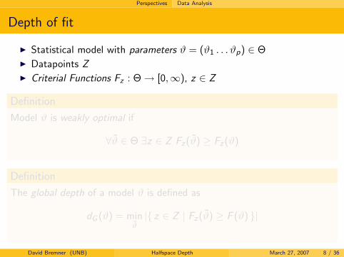
Perspectives Data Analysis
Depth of fit
I Statistical model with parameters ϑ = (ϑ1 . . . ϑp) ∈ ΘI Datapoints ZI Criterial Functions Fz : Θ→ [0,∞), z ∈ Z
Definition
Model ϑ is weakly optimal if
∀ϑ̃ ∈ Θ ∃z ∈ Z Fz(ϑ̃) ≥ Fz(ϑ)
Definition
The global depth of a model ϑ is defined as
dG (ϑ) = minϑ̃|{ z ∈ Z | Fz(ϑ̃) ≥ F (ϑ) }|
David Bremner (UNB) Halfspace Depth March 27, 2007 8 / 36

Perspectives Data Analysis
Linearization
Definition
For Fz differentiable, define the tangent depth of ϑ as
dT (ϑ) = minu 6=0|{ z | 〈 u,∇Fz(ϑ) 〉 ≥ 0 }|
Theorem (Mizera 2002)
If the Fz are differentiable and convex, and Θ ⊂ Rp is open and convex,then for any model ϑ ∈ Θ
dG (ϑ) = dT (ϑ)
David Bremner (UNB) Halfspace Depth March 27, 2007 9 / 36

Perspectives Data Analysis
Example: Two Factor ANOVA
I Two different experimental factors with levels in N = { 1 . . . n } andM = { 1 . . .m }.
I For each experimental setting (i , j) we have r data pointszi ,j ,1 . . . zi ,j ,r measuring outcomes.
Fertilizersoil 1 2
1 2 1
2 5 5
For simplicity, here r = 1
I The subset { zi ,j ,k | k = 1 . . . r } corresponding to an experimentalscenario is fit to some linear function f (ϑ) = µi + νj .
David Bremner (UNB) Halfspace Depth March 27, 2007 10 / 36

Perspectives Data Analysis
ANOVA example continued: Criterial Functions
Fertilizersoil ν1 = 1 ν2 = 2
µ1 = 1 2 1
µ2 = 2 5 5
I Parameter vector ϑ = (µ1 . . . µn, ν1 . . . νm).
I Criterial functions
Fi ,j ,k(ϑ) =(zi ,j ,k − (µi + νj))
2
2
I ∇Fi ,j ,k(ϑ) = −(zi ,j ,k − µi − µj)(ei , ej)
David Bremner (UNB) Halfspace Depth March 27, 2007 11 / 36

Perspectives Data Analysis
ANOVA example continued: scaled gradients
Scaling gradients
Recall ∇Fi ,j ,k(ϑ) = −(zi ,j ,k − µi − µj)(ei , ej).For purposes of computing depth, we may consider
Gi ,j ,k(ϑ) = − sign(zi ,j ,k − µi − µj)(ei , ej)
Fertilizersoil ν1 = 1 ν2 =
µ1 = 1 2 1
µ2 = 5 5
Gi ,j(1, 2, 1, 2)j
i 1 2
1 (0, 0, 0, 0) (1, 0, 0, 1)
2
depthZ (0) =
David Bremner (UNB) Halfspace Depth March 27, 2007 12 / 36

Perspectives Data Analysis
ANOVA example continued: scaled gradients
Scaling gradients
Recall ∇Fi ,j ,k(ϑ) = −(zi ,j ,k − µi − µj)(ei , ej).For purposes of computing depth, we may consider
Gi ,j ,k(ϑ) = − sign(zi ,j ,k − µi − µj)(ei , ej)
Fertilizersoil ν1 = 1 ν2 = 2
µ1 = 1 2 1
µ2 = 2 5 5
Gi ,j(1, 2, 1, 2)j
i 1 2
1 (0, 0, 0, 0) (1, 0, 0, 1)
2 − (0, 1, 1, 0) − (0, 1, 0, 1)
depthZ (0) = 1
David Bremner (UNB) Halfspace Depth March 27, 2007 12 / 36

Perspectives Data Analysis
ANOVA example continued: scaled gradients
Scaling gradients
Recall ∇Fi ,j ,k(ϑ) = −(zi ,j ,k − µi − µj)(ei , ej).For purposes of computing depth, we may consider
Gi ,j ,k(ϑ) = − sign(zi ,j ,k − µi − µj)(ei , ej)
Fertilizersoil ν1 = 1 ν2 = 1
µ1 = 1 2 1
µ2 = 4 5 5
Gi ,j(1, 4, 1, 1)j
i 1 2
1 (0, 0, 0, 0) (1, 0, 0, 1)
2 (0, 0, 0, 0) (0, 0, 0, 0)
depthZ (0) = 3
David Bremner (UNB) Halfspace Depth March 27, 2007 12 / 36
Perspectives Linear Inequality Systems
PerspectivesLocation EstimationData AnalysisLinear Inequality Systems
Approaches
Experimental Results
The Future
Bibliography
David Bremner (UNB) Halfspace Depth March 27, 2007 13 / 36

Perspectives Linear Inequality Systems
Maximum feasible subsystem
I Maximum Feasible Subsystem
Given Infeasible system Ax < 0Find A maximum subsystem of rows { 〈 ai , x 〉 < 0 | i ∈ I }
that is feasible
I MaxFS APX-hard Amaldi and Kann, 1998
I MaxFS and halfspace depth are equivalent
minu 6=0|{ p ∈ S | 〈 u, p 〉 ≥ 0 }| = |S | −max
u|{ p ∈ S | 〈 u, p 〉 < 0 }
Note condition u 6= 0 is unnecessary for strict MaxFS.
I Halfspace depth is APX-hard.
David Bremner (UNB) Halfspace Depth March 27, 2007 14 / 36

Approaches Enumeration without extra storage
Perspectives
ApproachesEnumeration without extra storagePrimal–Dual AlgorithmsA Fixed Parameter Tractable AlgorithmBranch and Cut
Experimental Results
The Future
Bibliography
David Bremner (UNB) Halfspace Depth March 27, 2007 15 / 36

Approaches Enumeration without extra storage
Traversing the dual arrangement
I Adj(X , j) is true iff negating sign j yields a cell. Test givenpolyhedron for interior. Solve via LP.
+ + ++
12
3
4
+ + +−
−+ +++ +−+
−+−+
−−++
Adj(+ + ++, 1) = true Adj(+ + ++, 2) = false
David Bremner (UNB) Halfspace Depth March 27, 2007 16 / 36
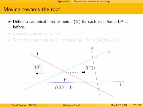
Approaches Enumeration without extra storage
Moving towards the root
I Define a canonical interior point i(X ) for each cell. Same LP asbefore.
I Choose an arbitrary cell C .
I To find a closer cell to C “shoot a ray” from i(X ) to i(C ).
12
3
4
i(C)i(X)
Y
f(X) = Y
David Bremner (UNB) Halfspace Depth March 27, 2007 17 / 36

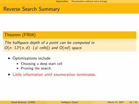
Approaches Enumeration without extra storage
Reverse Search Summary
Theorem (FR04)
The halfspace depth of a point can be computed inO(n · LP(n, d) · (# cells)) and O(nd) space.
I Optimizations includeI Choosing a deep start cellI Pruning the search.
I Little information until enumeration terminates.
David Bremner (UNB) Halfspace Depth March 27, 2007 18 / 36

Approaches Primal–Dual Algorithms
Perspectives
ApproachesEnumeration without extra storagePrimal–Dual AlgorithmsA Fixed Parameter Tractable AlgorithmBranch and Cut
Experimental Results
The Future
Bibliography
David Bremner (UNB) Halfspace Depth March 27, 2007 19 / 36

Approaches Primal–Dual Algorithms
Primal–Dual Algorithms
I Update at a every step an upper bound and a lower bound for thedepth.
I Terminate when (if) bounds are equal
I To ensure termination, fall back on enumeration after a fixed timelimit.
I Generally, answers improve with time.
David Bremner (UNB) Halfspace Depth March 27, 2007 20 / 36

Approaches Primal–Dual Algorithms
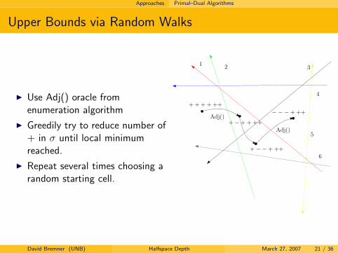
Upper Bounds via Random Walks
I Use Adj() oracle fromenumeration algorithm
I Greedily try to reduce number of+ in σ until local minimumreached.
I Repeat several times choosing arandom starting cell.
Adj()
Adj()
1 2 3
4
5
+ + + + ++
+−+ + ++
+−−+ ++
−−−+ ++
6
David Bremner (UNB) Halfspace Depth March 27, 2007 21 / 36

Approaches Primal–Dual Algorithms
Upper Bounds via Random Walks
I Use Adj() oracle fromenumeration algorithm
I Greedily try to reduce number of+ in σ until local minimumreached.
I Repeat several times choosing arandom starting cell.
Adj()
Adj()
1 2 3
4
5
+ + + + ++
+−+ + ++
+−−+ ++
−−−+ ++
6
David Bremner (UNB) Halfspace Depth March 27, 2007 21 / 36

Approaches Primal–Dual Algorithms
Upper Bounds Via Chinneck’s Heuristic
I Elasticize: aTi x < 0⇒ aT
i x − ηi < 0, η ≥ 0
I Solve LP, minSINF =∑
ηi
I For each constraint j with ηj > 0, remove and resolve.
I Permanently remove the constraint that most improved SINF
η1
η2
η3
David Bremner (UNB) Halfspace Depth March 27, 2007 22 / 36

Approaches Primal–Dual Algorithms
Lower Bounds via Minimal Dominating Sets
Definition
A Minimal Dominating Set (MDS) forp ∈ Rd with respect to S ⊂ Rd is R ⊆ Ssuch that
I p ∈ conv R
I if R ′ ( R then p /∈ conv R ′.
p
Proposition
Let ∆ be the set of all MDS’s for p with respect to S. Let T be aminimum transversal (hitting set) of ∆.
|T | = depth(p)
David Bremner (UNB) Halfspace Depth March 27, 2007 23 / 36

Approaches Primal–Dual Algorithms
Generating Missed MDSs (cuts)
Definition
Given a partial traversal T for the MDS’s of p w.r.t. S , define S̄ = S \ T .Define the auxiliary polytope Q(p,T ) as λ satisfying:
λS̄ = p∑i
λi = 1 λi ≥ 0
I Each vertex (basic solution) of Q(p,T ) defines an MDS missed by T .
I A single cut can be found by LP
I k cuts can be found via reverse search (or other pivoting method).
David Bremner (UNB) Halfspace Depth March 27, 2007 24 / 36

Approaches Primal–Dual Algorithms
Primal–Dual Algorithm
Implemented (BFR06) using ZRAM, cddlib, lrslib
1. Find candidate cell in the dual arrangement by upper bound heuristic
2. Find obstructions (i.e. MDS’s) to the optimality of this cell
3. If none found, report optimal (we have solved the global minimumtransversal problem).
4. Otherwise solve the resulting (partial) hitting set problem (or just findlower bound)
5. If bored, switch to enumeration.
David Bremner (UNB) Halfspace Depth March 27, 2007 25 / 36

Approaches A Fixed Parameter Tractable Algorithm
Perspectives
ApproachesEnumeration without extra storagePrimal–Dual AlgorithmsA Fixed Parameter Tractable AlgorithmBranch and Cut
Experimental Results
The Future
Bibliography
David Bremner (UNB) Halfspace Depth March 27, 2007 26 / 36

Approaches A Fixed Parameter Tractable Algorithm
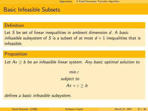
Basic Infeasible Subsets
Definition
Let S be set of linear inequalities in ambient dimension d . A basicinfeasible subsystem of S is a subset of at most d + 1 inequalities that isinfeasible.
Proposition
Let Ax ≥ b be an infeasible linear system. Any basic optimal solution to
min ε
subject to
Ax + ε ≥ b
defines a basic infeasible subsystem.
David Bremner (UNB) Halfspace Depth March 27, 2007 27 / 36
Approaches A Fixed Parameter Tractable Algorithm
Basic Infeasible Subsets
Definition
Let S be set of linear inequalities in ambient dimension d . A basicinfeasible subsystem of S is a subset of at most d + 1 inequalities that isinfeasible.
Proposition
Let Ax ≥ b be an infeasible linear system. Any basic optimal solution to
min ε
subject to
Ax + ε ≥ b
defines a basic infeasible subsystem.
David Bremner (UNB) Halfspace Depth March 27, 2007 27 / 36

Approaches A Fixed Parameter Tractable Algorithm
Bounded depth exhaustive search
Algorithm MFS(H : halfspaces, k : integer)
B ← BIS(H)if B = ∅ then return trueif k = 0 then return falsefor h ∈ B do
if MFS(H \ h, k − 1) = true then return trueendforreturn false
end
Theorem (BCILM06)
The halfspace depth of a point p with respect to a set S of n points in Rd
can be computed in O((d + 1)kLP(n, d − 1)) time, where k is the value ofthe output.
David Bremner (UNB) Halfspace Depth March 27, 2007 28 / 36

Approaches Branch and Cut
Perspectives
ApproachesEnumeration without extra storagePrimal–Dual AlgorithmsA Fixed Parameter Tractable AlgorithmBranch and Cut
Experimental Results
The Future
Bibliography
David Bremner (UNB) Halfspace Depth March 27, 2007 29 / 36

Approaches Branch and Cut
Branch and Cut
Root Node
SolvingLP
SolvingLP
SolvingLP
SolvingLP
SolvingLP
si = 1
sj = 0
si = 0
sj = 1
Adding Cuts
Adding Cuts
Adding Cuts Adding Cuts
Adding Cuts
x1
x2
cut
David Bremner (UNB) Halfspace Depth March 27, 2007 30 / 36

Approaches Branch and Cut
MIP formulation
Max Feasible Subsystem Problem
maxx|{ ai ∈ A | 〈 ai , x 〉 < 0 }|
Mixed Integer Program
min∑
i
si
subj. to
〈 ai , x 〉 − siM + ε ≤ 0
David Bremner (UNB) Halfspace Depth March 27, 2007 31 / 36

Approaches Branch and Cut
MIP formulation
Max Feasible Subsystem Problem
maxx|{ ai ∈ A | 〈 ai , x 〉 < 0 }|
Mixed Integer Program
min∑
i
si
subj. to
〈 ai , x 〉 − siM + ε ≤ 0
David Bremner (UNB) Halfspace Depth March 27, 2007 31 / 36

Approaches Branch and Cut
Branch and cut details
I Implementation by Dan Chen, using tools from COIN-OR.
I Chinneck’s heuristic algorithm is used to find an initial upper bound
I MDS/BIS used as cutting planes.
I Binary-search version “eliminates” ε
I Various branching heuristics available.
David Bremner (UNB) Halfspace Depth March 27, 2007 32 / 36

Experimental Results
Random Data
Comparison of the branch and cut, binary search, and primal−dual algorithm
Data sets of 50 points
dataset (dimension / depth)
11/2
12/2
12/3 8/4
12/4 8/5
10/4
3/12
11/5 9/5
10/5 7/7
4/11 5/
9
4/12
10/6
3/18
3/18
(2)
7/8
6/10
4/16
11/6 9/8
5/13
5/13
(2)
6/11
6/14 9/
9
7/11
8/11
cput
ime
1s
10s
1m
4m
10m
20m30m
1h
2h
10h B&C
B−S
P−D
David Bremner (UNB) Halfspace Depth March 27, 2007 33 / 36

Experimental Results
ANOVA Datacp
utim
e
1s
10s
1m
4m
30m
0 5 10 15 20 25 30 35 40 45
4 x 4 x 2
4 x 4 x 3
4 x 4 x 4
6 x 6 x 2
6 x 6 x 3
6 x 6 x 4
David Bremner (UNB) Halfspace Depth March 27, 2007 34 / 36
The Future
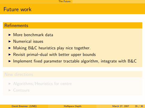
Future work
Refinements
I More benchmark data
I Numerical issues
I Making B&C heuristics play nice together.
I Revisit primal–dual with better upper bounds
I Implement fixed parameter tractable algorithm, integrate with B&C
New directions
I Algorithms/Heuristics for centre
I Contours
David Bremner (UNB) Halfspace Depth March 27, 2007 35 / 36

The Future
Future work
Refinements
I More benchmark data
I Numerical issues
I Making B&C heuristics play nice together.
I Revisit primal–dual with better upper bounds
I Implement fixed parameter tractable algorithm, integrate with B&C
New directions
I Algorithms/Heuristics for centre
I Contours
David Bremner (UNB) Halfspace Depth March 27, 2007 35 / 36

Bibliography
Bibliography
David Bremner, Dan Chen, John Iacono, Stefan Langerman, and Pat Morin.
Output-sensitive algorithms for Tukey depth and related problems.Submitted, September 2006.
David Bremner, Komei Fukuda, and Vera Rosta.
Primal dual algorithms for data depth.In Reginia Y. Liu, Robert Serfling, and Diane L. Souvaine, editors, Data Depth: Robust Multivariate Analysis,Computational Geometry, and Applications, volume 72 of AMS DIMACS Book Series, pages 171–194. January 2006.
Dan Chen.
A branch and cut algorithm for the halfspace depth problem.Master’s thesis, UNB, 2007.
John Chinneck.
Fast heuristics for the maximum feasible subsystem problem.INFORMS J. Computing, 13(3):210–223, 2001.
K. Fukuda and V. Rosta.
Exact parallel algorithms for the location depth and the maximum feasible subsystem problems.In Frontiers in global optimization, volume 74 of Nonconvex Optim. Appl., pages 123–133. Kluwer Acad. Publ., Boston,MA, 2004.
Ivan Mizera.
On depth and deep points: a calculus.Ann. Statist., 30(6):1681–1736, 2002.
David Bremner (UNB) Halfspace Depth March 27, 2007 36 / 36


![BREMNER L. [Reframing Township Space. the Kliptown Project]](https://static.documents.pub/doc/80x56/577cd1ce1a28ab9e7895022f/bremner-l-reframing-township-space-the-kliptown-project.jpg)


