ATA Memo 75 1 Handbook of 1.4 GHz Phase Calibrators for ATA G. R. Harp This document is a reference for choosing phase calibrators at the ATA. Simulated snapshots of the 70 brightest source fields are shown, along with information relating to their suitability for calibration at different frequencies. The simulations are based upon the NRAO VLA Sky Survey which was performed at 1.42 GHz. At other frequencies (e.g. 5 GHz) this book is still helpful as guidance, though calibrators must themselves be characterized for accurate work. Introduction The ATA is unique because of its large field of view (FOV) in the cm wavelength range; e.g. 2.5° diameter to the half-power point at 1.42 GHz, and approximately 5° diameter to the first primary beam minimum. The large FOV is an important reason why the ATA is excellent for survey work and measurement of large scale structures on the sky. To effectively use the ATA, we must re-think our usual procedures relating to calibration because the large FOV means that no point source on the sky can really be considered isolated from background sources. As we show in the pages of this book, even strong continuum sources like Virgo A have enough integrated flux in their vicinity to make simple, point source calibration dubious. In this memo we characterize potential calibrators by simulating 5 degree fields surrounding 70 bright sources. The simulations use the NRAO VLA Sky Survey (NVSS) catalog which contains approximately 1.8 million point sources with flux densities as low as 2.5 mJy. The observations for NVSS had approximately 0.75’ resolution. [J. J. Condon, et al. (1998), “The NRAO VLA Sky Survey,” Astrophysical Journal. 115: 1693.] It is worth noting that the NVSS catalog may be browsed directly at http://www.cv.nrao.edu/nvss/NVSSlist.shtml where source lists are generated surrounding a designated target. These simulations are generated by first choosing a bright source which serves as the field center. The sources of the NVSS catalog are culled to retain only those within the primary field of view, which is simulated by a 2.46° full width at half maximum (FWHM) Gaussian. The retained flux densities are weighted by the simulated primary beam pattern and each point source convolved with a Gaussian synthetic beam having FWHM of 1’, which is slightly smaller than the expected ATA 350 synthetic beam diameter of 1.5’ at 1.42 GHz. This book is organized with one bright calibrator per page and ordered by increasing right-ascension of the source. On each page is an image of the calibrator and some information regarding its suitability for phase calibration as a function of primary beam diameter. Primary beam diameter (FWHM) can be approximately related to frequency f using the following formula
Transcript
ATA Memo 75
1
Handbook of 1.4 GHz Phase Calibrators for ATA G. R. Harp
This document is a reference for choosing phase calibrators at the ATA. Simulated snapshots of the 70 brightest source fields are shown, along with information relating to their suitability for
calibration at different frequencies. The simulations are based upon the NRAO VLA Sky Survey which was performed at 1.42 GHz. At other frequencies (e.g. 5 GHz) this book is still helpful as
guidance, though calibrators must themselves be characterized for accurate work.
Introduction The ATA is unique because of its large field of view (FOV) in the cm wavelength range; e.g. 2.5° diameter to the half-power point at 1.42 GHz, and approximately 5° diameter to the first primary beam minimum. The large FOV is an important reason why the ATA is excellent for survey work and measurement of large scale structures on the sky. To effectively use the ATA, we must re-think our usual procedures relating to calibration because the large FOV means that no point source on the sky can really be considered isolated from background sources. As we show in the pages of this book, even strong continuum sources like Virgo A have enough integrated flux in their vicinity to make simple, point source calibration dubious. In this memo we characterize potential calibrators by simulating 5 degree fields surrounding 70 bright sources. The simulations use the NRAO VLA Sky Survey (NVSS) catalog which contains approximately 1.8 million point sources with flux densities as low as 2.5 mJy. The observations for NVSS had approximately 0.75’ resolution. [J. J. Condon, et al. (1998), “The NRAO VLA Sky Survey,” Astrophysical Journal. 115: 1693.] It is worth noting that the NVSS catalog may be browsed directly at http://www.cv.nrao.edu/nvss/NVSSlist.shtml where source lists are generated surrounding a designated target. These simulations are generated by first choosing a bright source which serves as the field center. The sources of the NVSS catalog are culled to retain only those within the primary field of view, which is simulated by a 2.46° full width at half maximum (FWHM) Gaussian. The retained flux densities are weighted by the simulated primary beam pattern and each point source convolved with a Gaussian synthetic beam having FWHM of 1’, which is slightly smaller than the expected ATA 350 synthetic beam diameter of 1.5’ at 1.42 GHz. This book is organized with one bright calibrator per page and ordered by increasing right-ascension of the source. On each page is an image of the calibrator and some information regarding its suitability for phase calibration as a function of primary beam diameter. Primary beam diameter (FWHM) can be approximately related to frequency f using the following formula
ATA Memo 75
2
DegGHz
3.5FWHMf
≅ . (1.1)
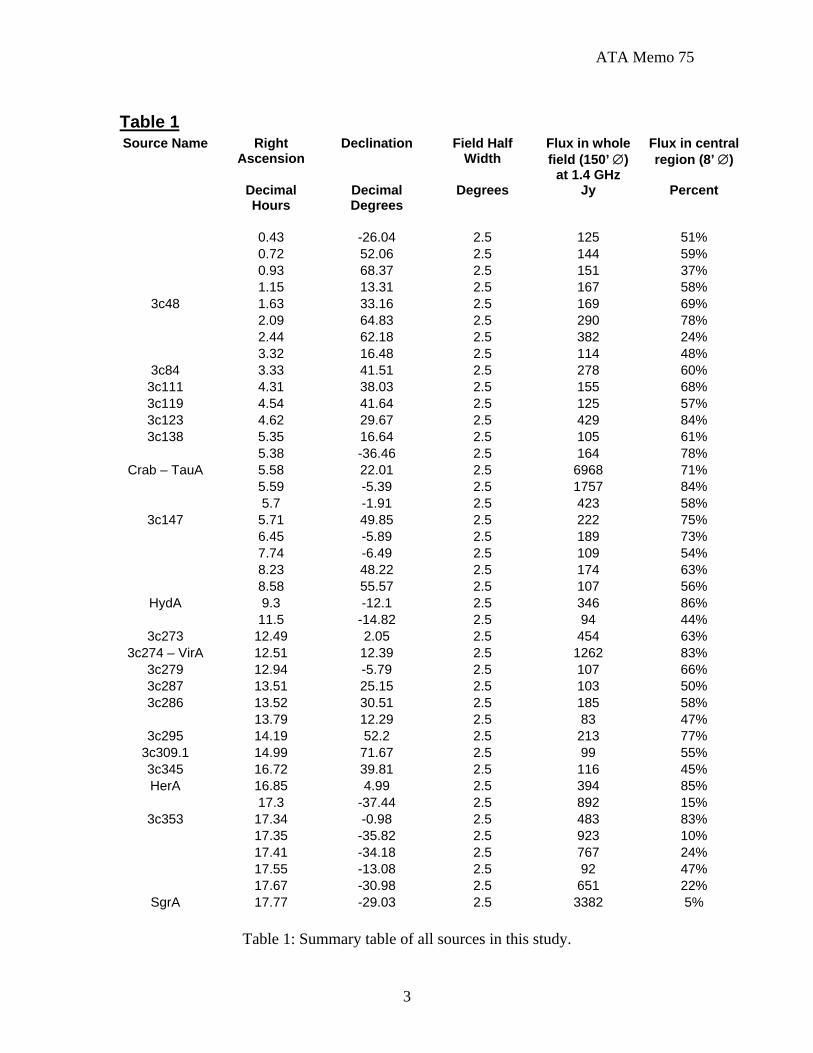
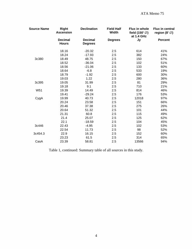
The sources were chosen by globally ordering the NVSS survey sources according to flux density and keeping the top 100 sources. In some cases, strong sources that are found to be close together, and the fields for these were combined into single fields centered at a position near the source ‘center of mass.’ The resultant list has about 70 independent fields. The data are summarized in Table 1. The table contains most of the brightest fields in the NVSS catalog down to around 100 Jy. Beyond the total (weighted) flux density in the 150’ field, the most important figure of merit is the flux density in the central region of the field. The central region is defined as a circle with 500” or approximately 8’ diameter. Despite the fact that these are the strongest VLA sources, the flux in this central region often cannot be called the overwhelmingly dominant source in the field. This is a fact that users of the ATA must face up to: when using “point source” calibrators to self-calibrate the telescope, it may be necessary to clean the calibrator in the image plane and iterate the calibration to optimize the results.
Table 1, continued: Summary table of all sources in this study.
ATA Memo 75
5
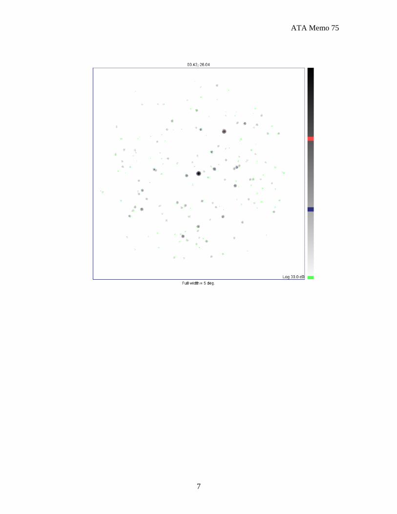
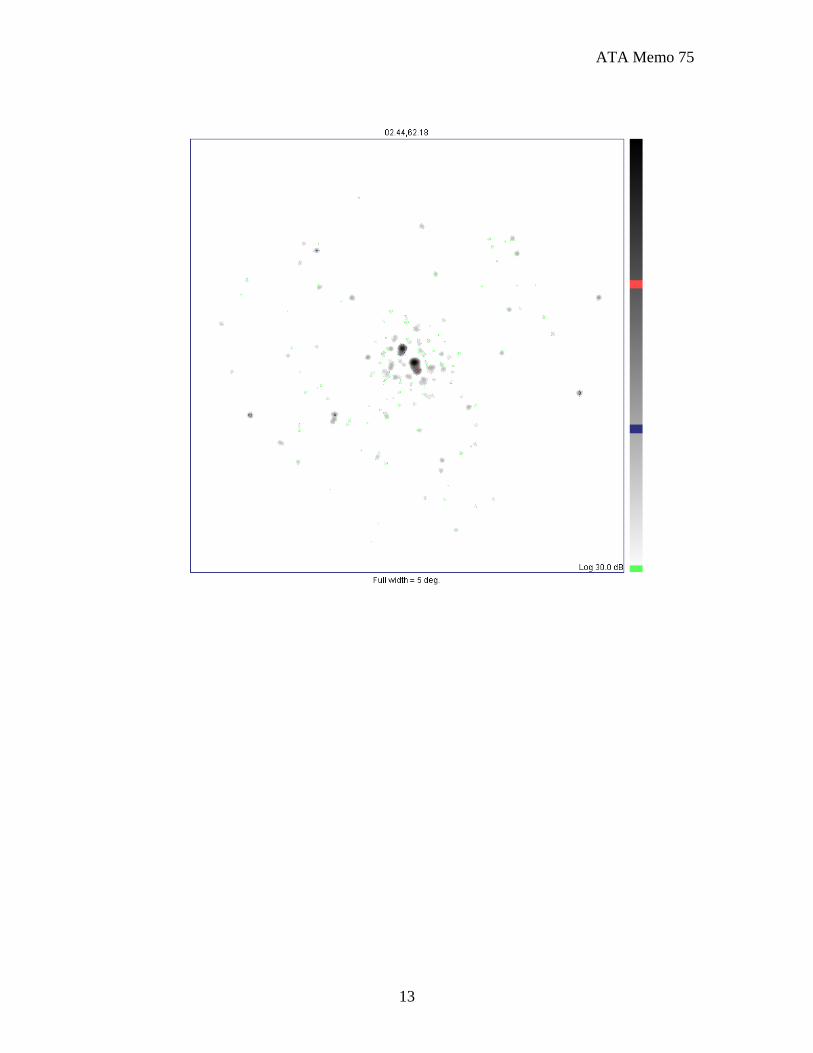
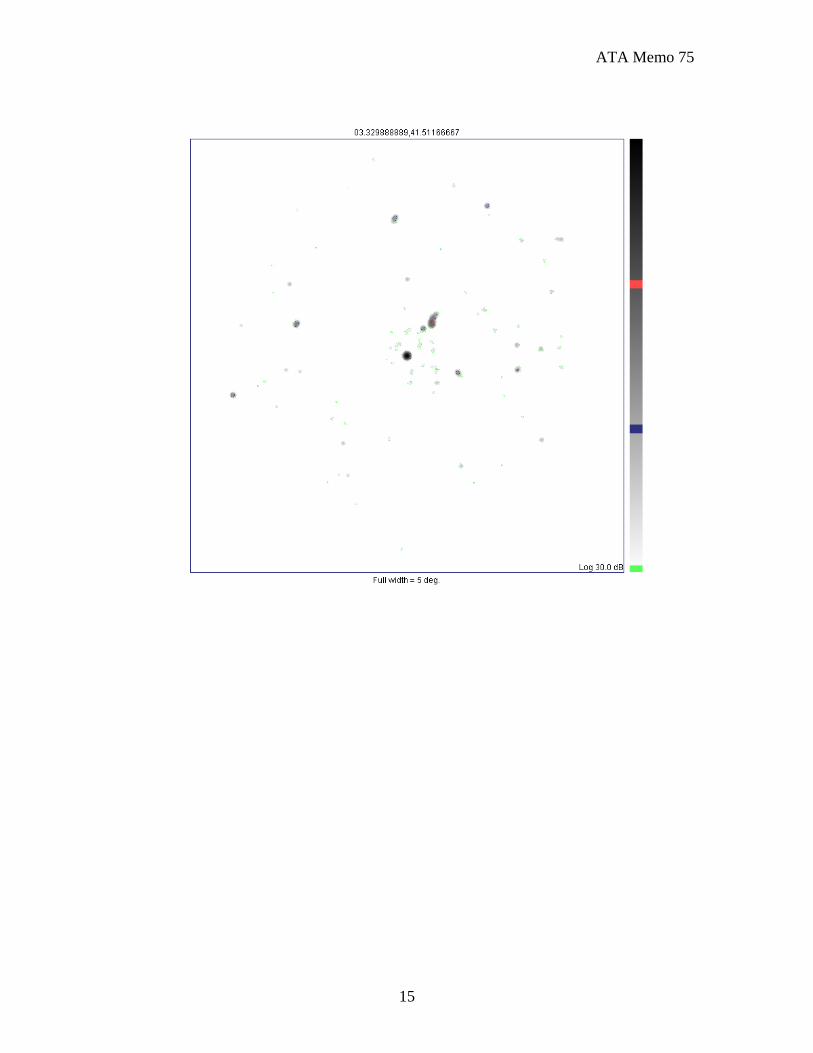
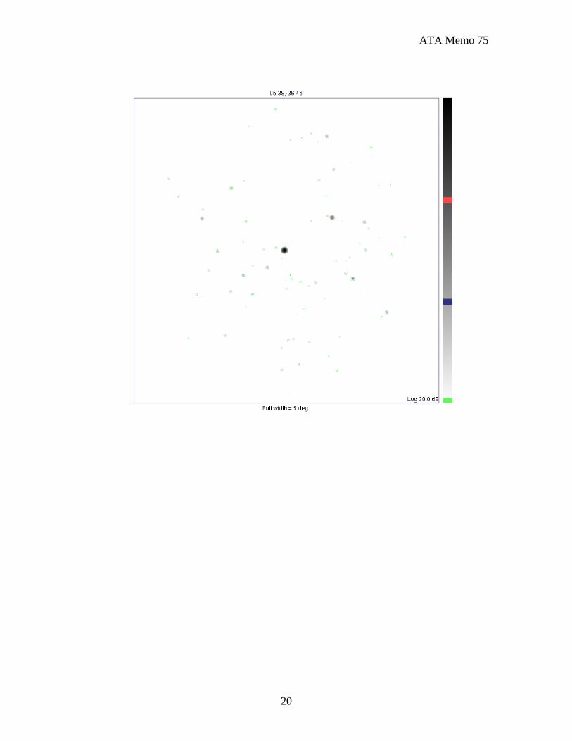
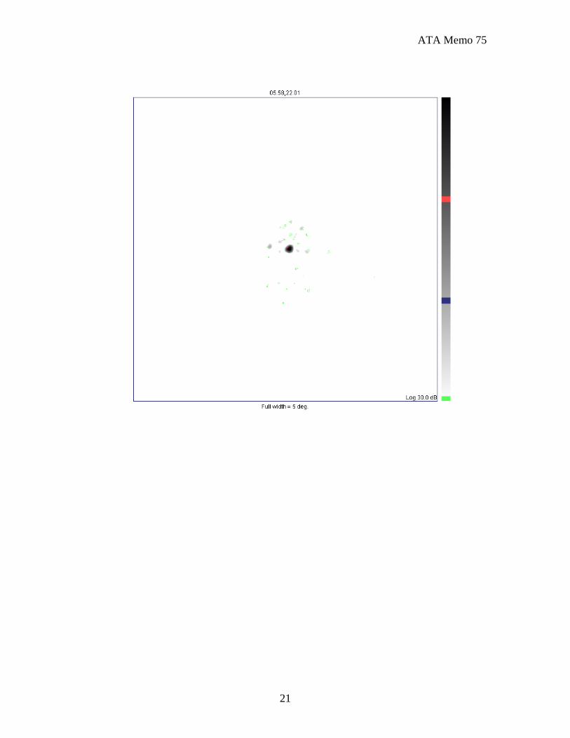
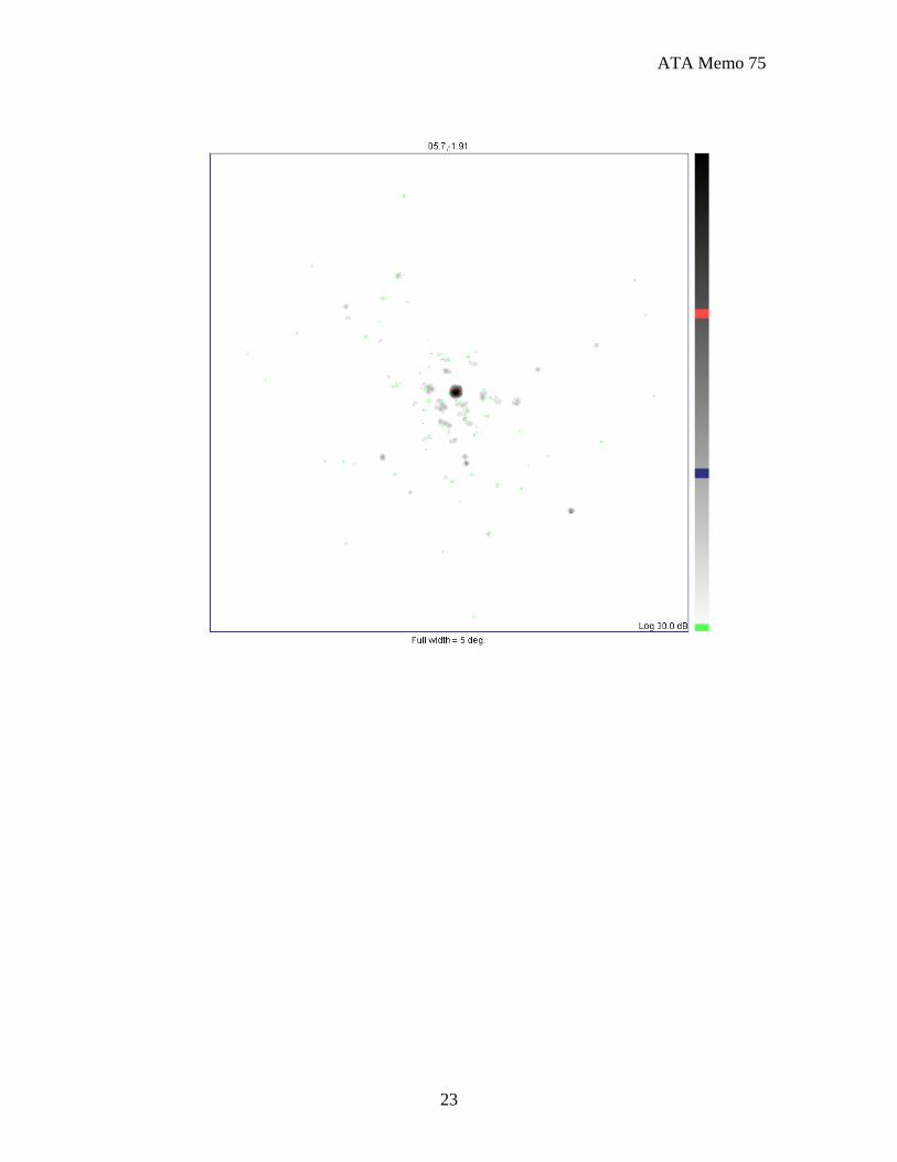
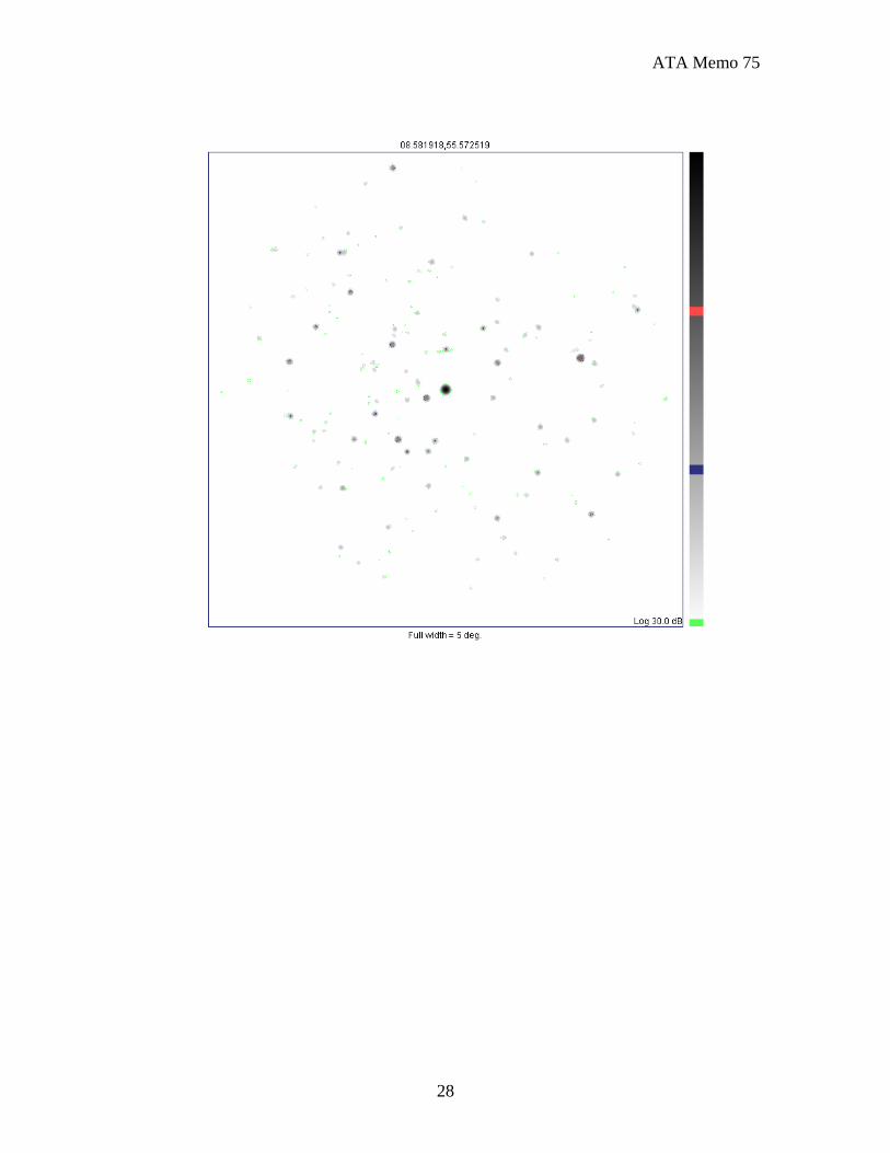
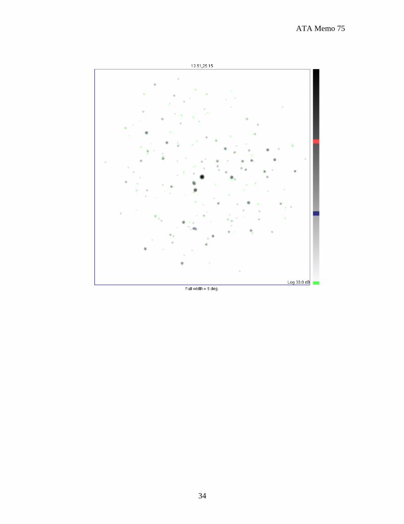
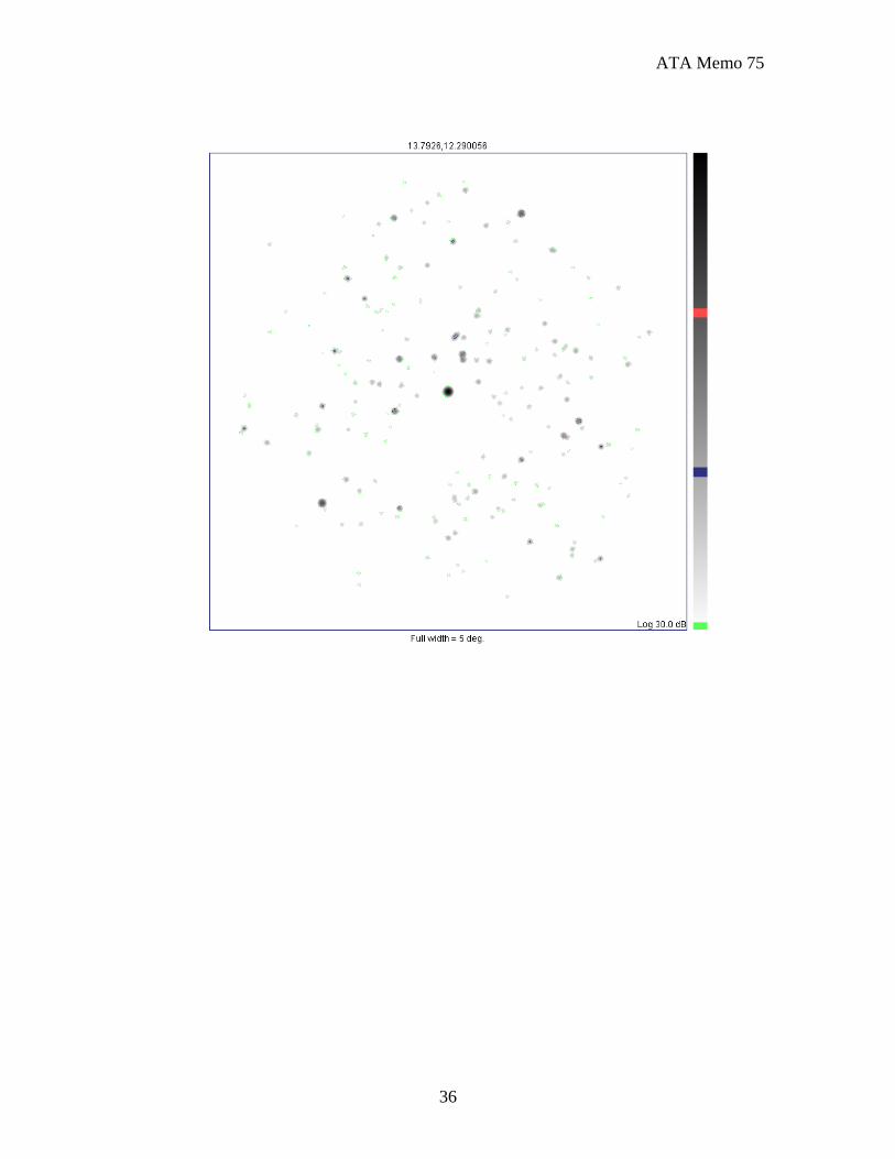
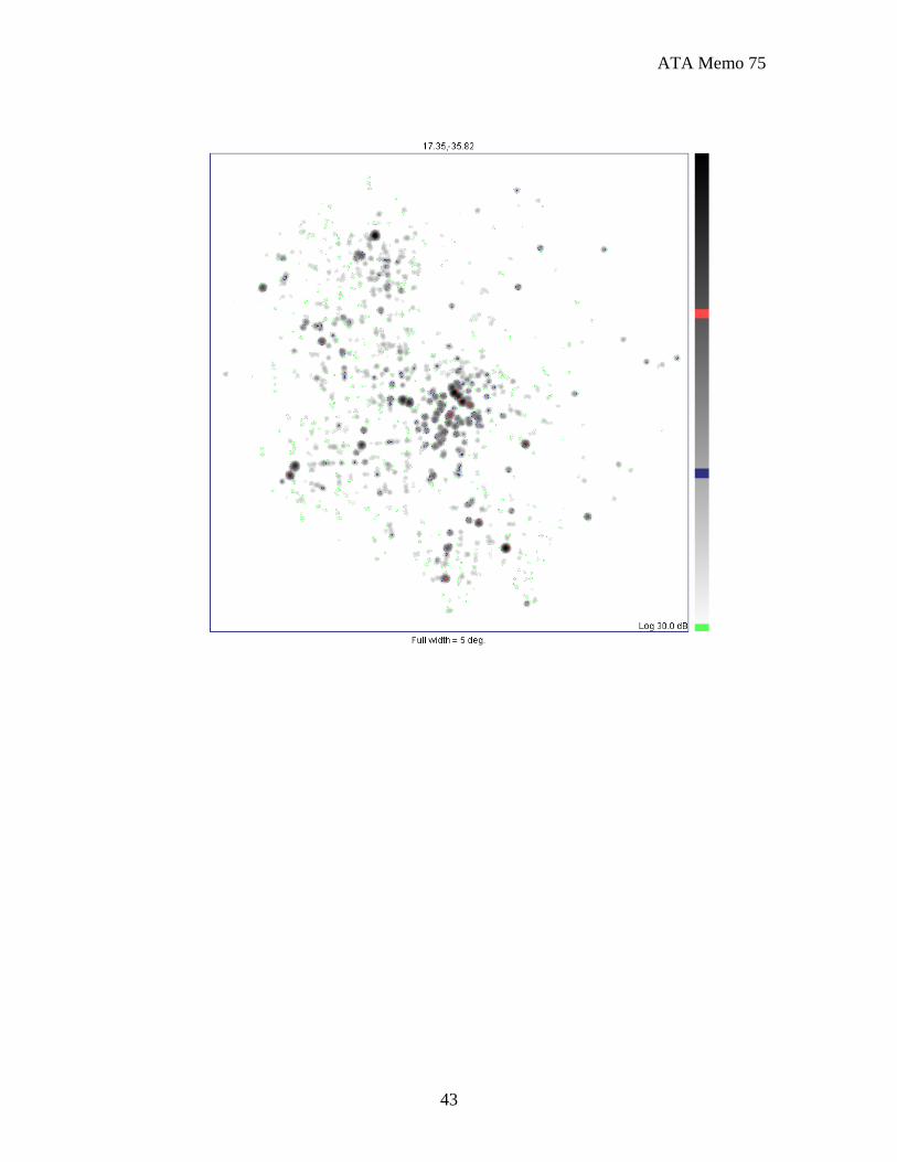
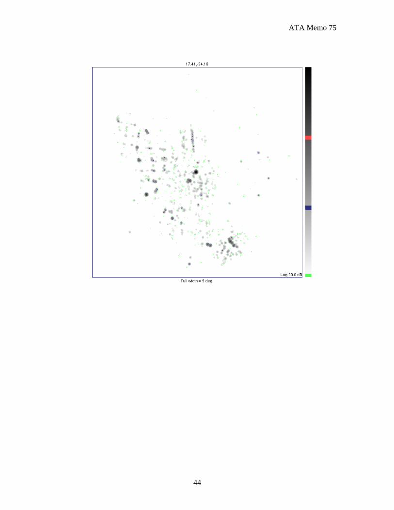
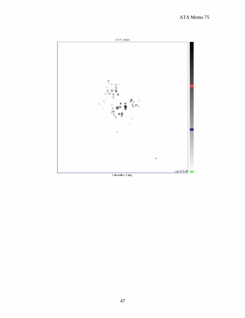
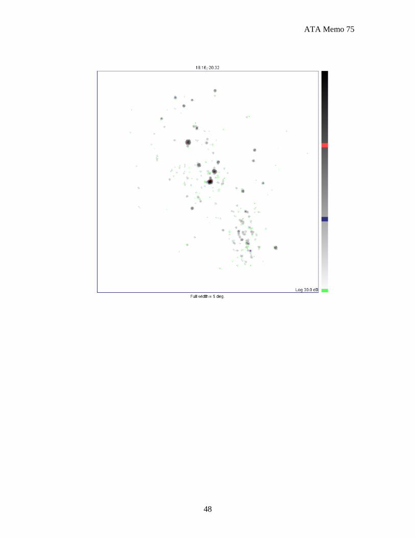
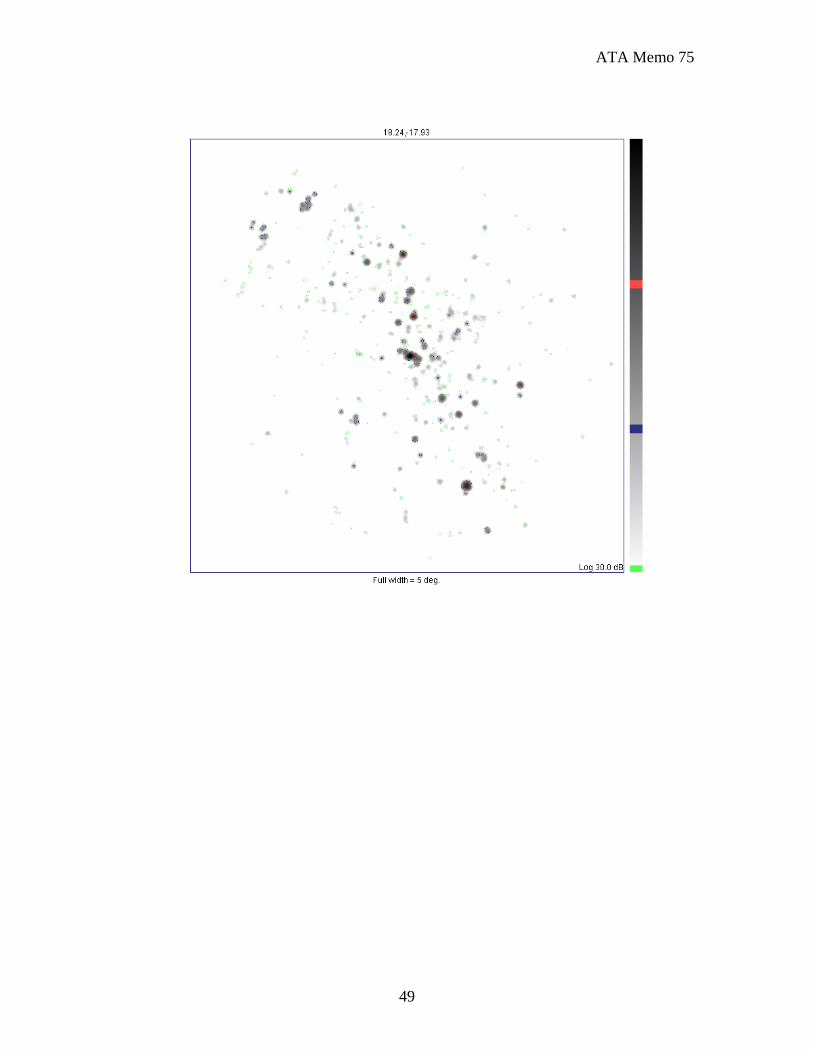
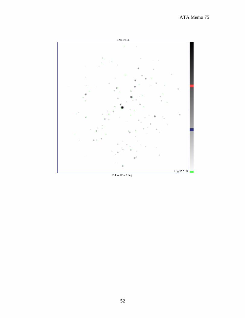
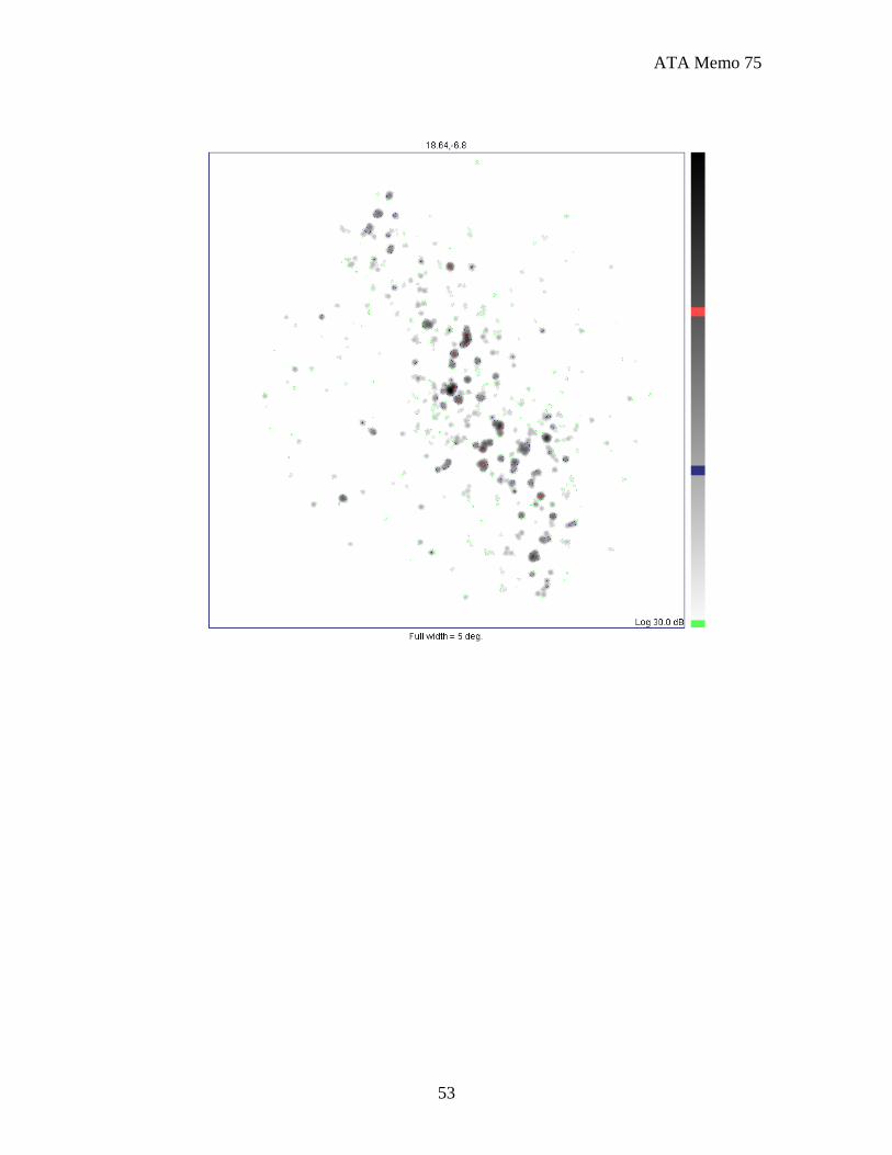
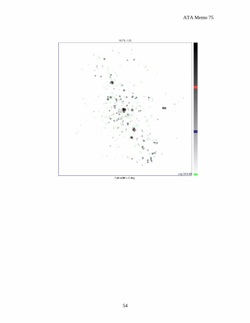
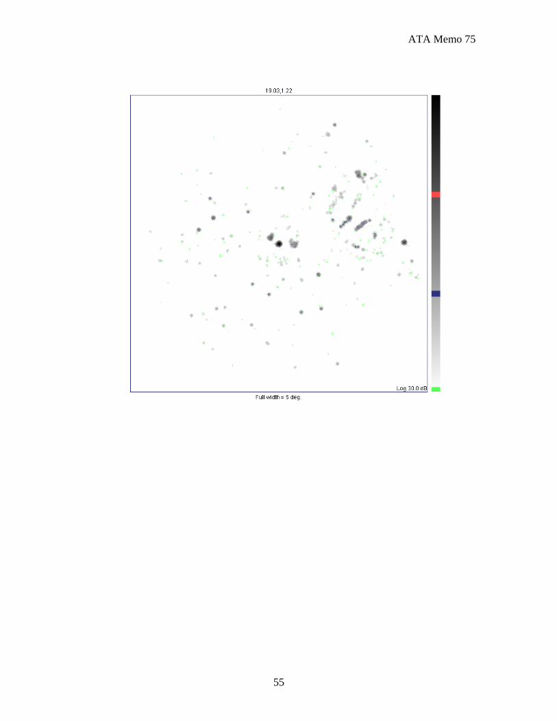
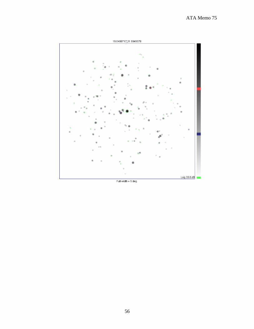
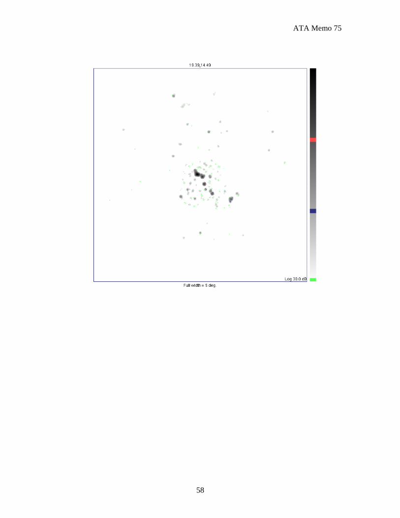
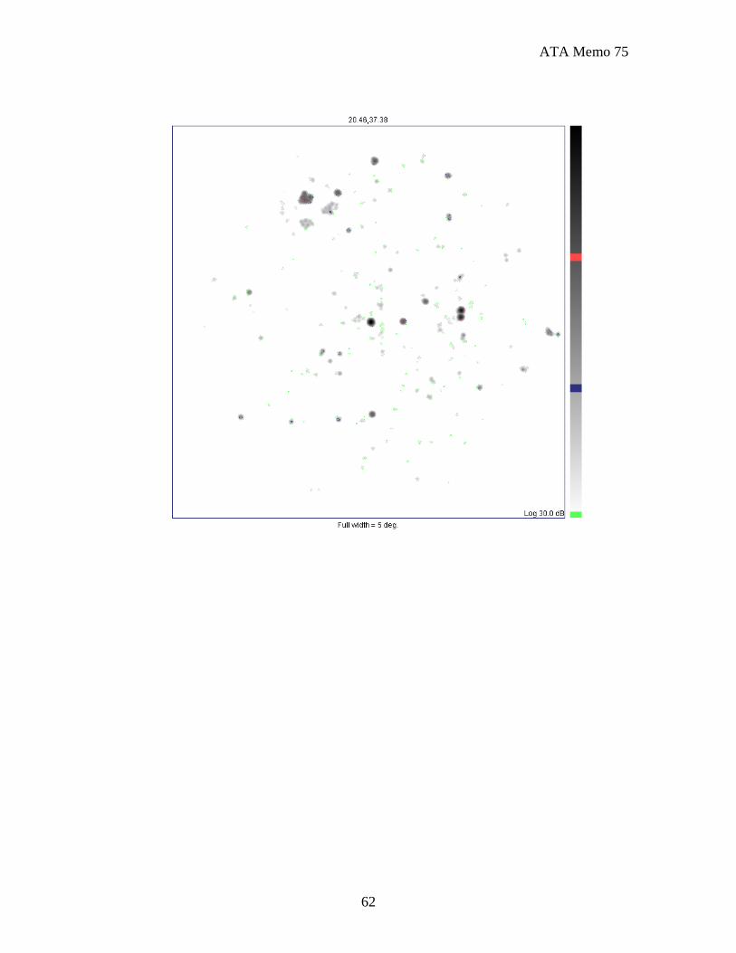
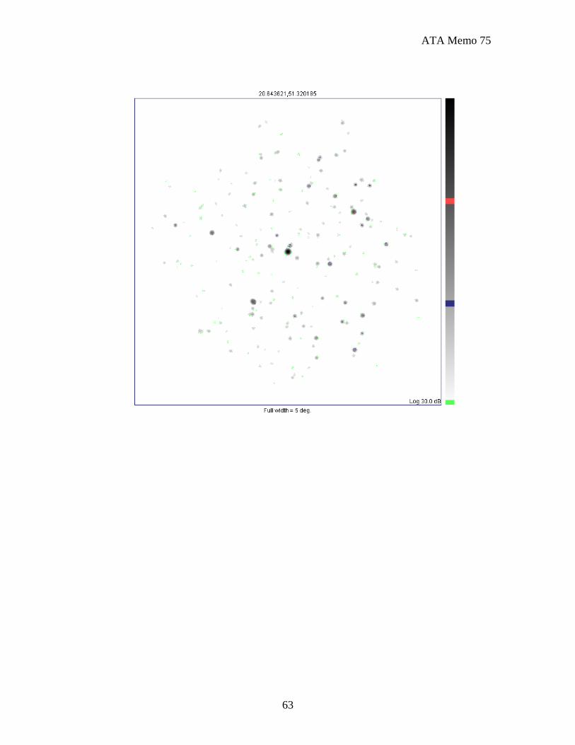
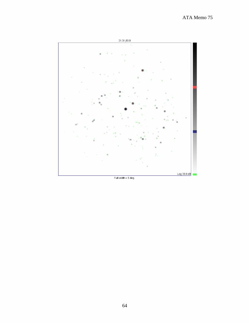
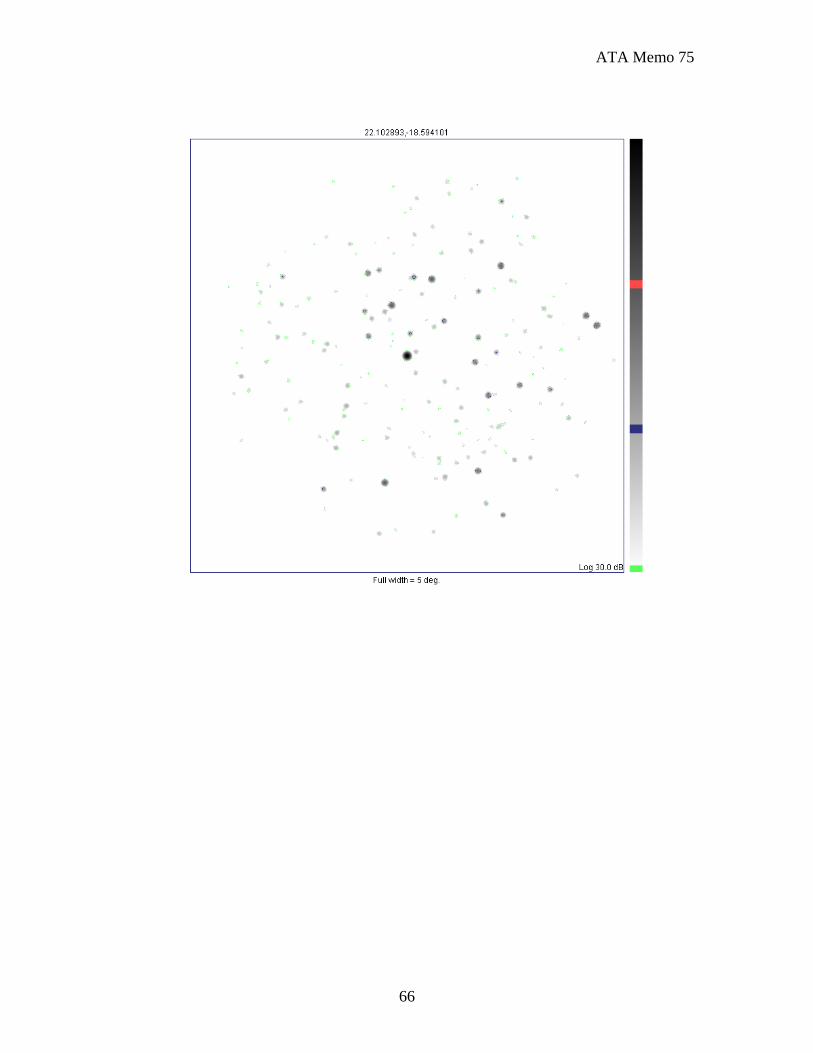
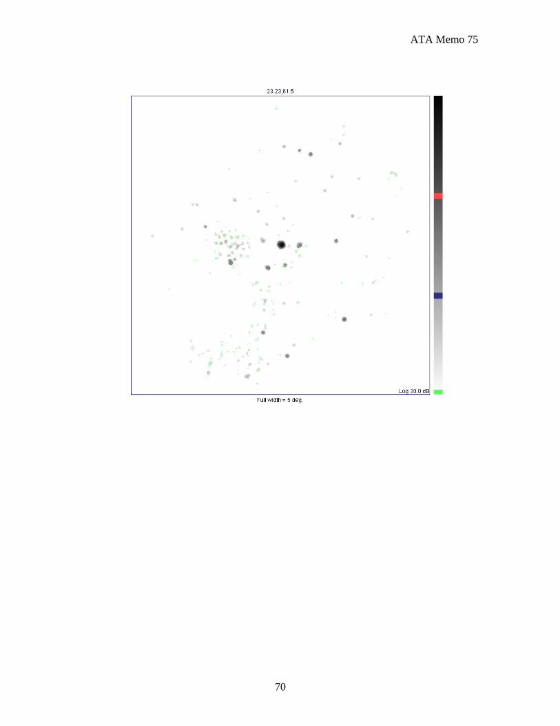
What follows below is a picture book of all the fields in Table 1, simulated from the NVSS catalog using the ATA primary beam at 1.42 GHz. Figure 1 points out the salient features of these images.
Figure 1: Example field from the picture book. All fields are displayed with a logarithmic gray scale spanning 30 dB. Three contour levels are shown in each image at -10 dB, -20 dB, and -30 dB relative to the peak intensity (generally, the peak is at image center).
How to use this book: First consult the table for a list of calibrators in the vicinity of your target field. Check the flux and center-flux to decide how long you may need to integrate on the calibrator to obtain good statistics. We don’t have the spectral index of these sources (yet), so at frequencies far from 1.42 GHz the relative brightness of the continuum sources in a field may change. Most extragalactic sources have a decreasing flux density with increasing frequency with spectral index = 0.7. Hence the loss in flux at frequency f may be estimated from
0.7GHz
GHzFlux at Flux at 1.42 GHz *1.42ff
−⎛ ⎞= ⎜ ⎟⎝ ⎠
.
(1.2) If you are observing at a frequency different from 1.42 GHz, estimate the ATA primary beam diameter using Eq. (1.1). You may wish to draw a circle on the calibrator image representing the full width of the ATA primary beam at your frequency. Examine the field images of these calibrators to see if there are strong sources at the edge of the field which may confuse the calibration. Remember that the ATA primary beam pattern is not
Full range of color bar
Field of View
Field center RA, Dec
ATA Memo 75
6
well characterized at the edge of the field, so calibrators with strong sources at the field edge should be avoided. Finally, you may wish to generate your own simulations of the continuum radiation at your chosen frequency for both your target field and your chosen calibrator. This can be done in the ATA control system using the command “atafield.” To begin, log in to one of the ATA control computers, type the command atafield at the command line prompt. This will display a list of options that may be used in the simulation. For example: atafield 11.501959,-14.824275 --fov 5.0 --size 640 --log 30 --negative This example was taken directly from the script that generated all of the images in this book. Change the FOV for your own frequency, and keep in mind that no matter what FOV you choose, the simulation is always at 1.42 GHz.
Citations: If you include substantive results of these simulations in a published paper, it is important to give credit to the authors of the NVSS survey by citing:
J. J. Condon, et al. (1998), “The NRAO VLA Sky Survey,” Astrophysical Journal. 115: 1693.
Similarly, you may make reference to this memo:
G. R. Harp (2007), “Handbook of 1.42 GHz phase calibrators for the ATA,” ATA Memo Series 75.
Acknowledgement: The author gratefully acknowledges Rick Forster for critical reading and several helpful additions to the text. The picture book follows.