Handbook of Monte Carlo Methods Dirk P. Kroese University of Queensland Thomas Taimre University of Queensland Zdravko I. Botev Université de Montréal WILEY A JOHN WILEY & SONS, INC., PUBLICATION
Transcript
Handbook of Monte Carlo Methods
Dirk P. Kroese University of Queensland
Thomas Taimre University of Queensland
Zdravko I. Botev Université de Montréal
WILEY A JOHN WILEY & SONS, INC., PUBLICATION
This page intentionally left blank
Handbook of Monte Carlo Methods
WILEY SERIES IN PROBABILITY AND STATISTICS
Established by WALTER A. SHEWHART and SAMUEL S. WILKS
Editors: David J. Balding, Noel A. C. Cressie, Garrett M. Fitzmaurice, Iain M. Johnstone, Geert Molenberghs, David W. Scott, Adrian F. M. Smith, Ruey S. Tsay, Sanford Weisberg Editors Emeriti: Vic Barnett, J. Stuart Hunter, Joseph B. Kadane, JozefL. Teugels
A complete list of the titles in this series appears at the end of this volume.
Published by John Wiley & Sons, Inc., Hoboken, New Jersey Published simultaneously in Canada
No part of this publication may be reproduced, stored in a retrieval system, or transmitted in any form or by any means, electronic, mechanical, photocopying, recording, scanning, or otherwise, except as permitted under Section 107 or 108 of the 1976 United States Copyright Act, without either the prior written permission of the Publisher, or authorization through payment of the appropriate per-copy fee to the Copyright Clearance Center, Inc., 222 Rosewood Drive, Danvers, MA 01923, (978) 750-8400, fax (978) 750-4470, or on the web at www.copyright.com. Requests to the Publisher for permission should be addressed to the Permissions Department, John Wiley & Sons, Inc., 111 River Street, Hoboken, NJ 07030, (201) 748-6011, fax (201) 748-6008, or online at http://www.wiley.com/go/permission.
Limit of Liability/Disclaimer of Warranty: While the publisher and author have used their best efforts in preparing this book, they make no representations or warranties with respect to the accuracy or completeness of the contents of this book and specifically disclaim any implied warranties of merchantability or fitness for a particular purpose. No warranty may be created or extended by sales representatives or written sales materials. The advice and strategies contained herein may not be suitable for your situation. You should consult with a professional where appropriate. Neither the publisher nor author shall be liable for any loss of profit or any other commercial damages, including but not limited to special, incidental, consequential, or other damages.
For general information on our other products and services or for technical support, please contact our Customer Care Department within the United States at (800) 762-2974, outside the United States at (317) 572-3993 or fax (317) 572-4002.
Wiley also publishes its books in a variety of electronic formats. Some content that appears in print may not be available in electronic formats. For more information about Wiley products, visit our web site at www.wiley.com.
Library of Congress Cataloging-in-Publication Data:
Kroese, Dirk P. Handbook for Monte Carlo methods / Dirk P. Kroese, Thomas Taimre, Zdravko I. Botev.
p. cm. — (Wiley series in probability and statistics ; 706) Includes index.
ISBN 978-0-470-17793-8 (hardback) 1. Monte Carlo method. I. Taimre, Thomas, 1983- II. Botev, Zdravko I., 1982- III. Title. QA298.K76 2011 518'.282—dc22 2010042348
12.4.1 Genetic Algorithms 452 12.4.2 Differential Evolution 454 12.4.3 Estimation of Distribution Algorithms 456
12.5 Cross-Entropy Method for Optimization 457 12.6 Other Randomized Optimization Techniques 460
References 461
13 Cross-Entropy Method 463
13.1 Cross-Entropy Method 463 13.2 Cross-Entropy Method for Estimation 464 13.3 Cross-Entropy Method for Optimization 468
13.3.1 Combinatorial Optimization 469
CONTENTS XIII
13.3.2 Continuous Optimization 471
13.3.3 Constrained Optimization 473
13.3.4 Noisy Optimization 476
References 477
14 Particle Methods 481
14.1 Sequential Monte Carlo 482
14.2 Particle Splitting 485
14.3 Splitting for Static Rare-Event Probability Estimation 486
14.4 Adaptive Splitting Algorithm 493
14.5 Estimation of Multidimensional Integrals 495
14.6 Combinatorial Optimization via Splitting 504
14.6.1 Knapsack Problem 505
14.6.2 Traveling Salesman Problem 506
14.6.3 Quadratic Assignment Problem 508
14.7 Markov Chain Monte Carlo With Splitting 509
References 517
15 Applications to Finance 521
15.1 Standard Model 521
15.2 Pricing via Monte Carlo Simulation 526
15.3 Sensitivities 538
15.3.1 Pathwise Derivative Estimation 540
15.3.2 Score Function Method 542
References 546
16 Applications to Network Reliability 549
16.1 Network Reliability 549
16.2 Evolution Model for a Static Network 551
16.3 Conditional Monte Carlo 554
16.3.1 Leap-Evolve Algorithm 560
16.4 Importance Sampling for Network Reliability 562
16.4.1 Importance Sampling Using Bounds 562
16.4.2 Importance Sampling With Conditional Monte Carlo 565
16.5 Splitting Method 567
16.5.1 Acceleration Using Bounds 573
References 574
17 Applications to Differential Equations 577
17.1 Connections Between Stochastic and Partial Differential
Equations 577
XIV CONTENTS
17.1.1 Boundary Value Problems 579
17.1.2 Terminal Value Problems 584
17.1.3 Terminal-Boundary Problems 585
17.2 Transport Processes and Equations 587
17.2.1 Application to Transport Equations 589
17.2.2 Boltzmann Equation 593
17.3 Connections to ODEs Through Scaling 597
References 602
Appendix A: Probability and Stochastic Processes 605
A.l Random Experiments and Probability Spaces 605
A. 1.1 Properties of a Probability Measure 607
A.2 Random Variables and Probability Distributions 607
A.2.1 Probability Density 610
A.2.2 Joint Distributions 611
A.3 Expectation and Variance 612
A.3.1 Properties of the Expectation 614
A.3.2 Variance 615
A.4 Conditioning and Independence 616
A.4.1 Conditional Probability 616
A.4.2 Independence 616
A.4.3 Covariance 617
A.4.4 Conditional Density and Expectation 618
A.5 W Space 619
A.6 Functions of Random Variables 620
A.6.1 Linear Transformations 620
A.6.2 General Transformations 620
A.7 Generating Function and Integral Transforms 621
A.7.1 Probability Generating Function 621
A.7.2 Moment Generating Function and Laplace Transform 621
A.7.3 Characteristic Function 622
A.8 Limit Theorems 623
A.8.1 Modes of Convergence 623
A.8.2 Converse Results on Modes of Convergence 624
A.8.3 Law of Large Numbers and Central Limit Theorem 625
A.9 Stochastic Processes 626
A.9.1 Gaussian Property 627
A.9.2 Markov Property 628
A.9.3 Martingale Property 629
A.9.4 Regenerative Property 630
A.9.5 Stationarity and Reversibility 631
A. 10 Markov Chains 632
CONTENTS XV
A.10.1 Classification of States 633
A.10.2 Limiting Behavior 633
A. 10.3 Reversibility 635
A. 11 Markov Jump Processes 635
A. 11.1 Limiting Behavior 638
A. 12 Itô Integral and Itô Processes 639
A.13 Diffusion Processes 643
A. 13.1 Kolmogorov Equations 646
A. 13.2 Stationary Distribution 648
A. 13.3 Feynman-Kac Formula 648
A.13.4 Exit Times 649
References 650
Appendix B: Elements of Mathematical Statistics 653
B.l Statistical Inference 653
B. l . l Classical Models 654
B.l.2 Sufficient Statistics 655
B.l . 3 Estimation 656
B.l.4 Hypothesis Testing 660
B.2 Likelihood 664
B.2.1 Likelihood Methods for Estimation 667
B.2.2 Numerical Methods for Likelihood Maximization 669
B.2.3 Likelihood Methods for Hypothesis Testing 671
B.3 Bayesian Statistics 672
B.3.1 Conjugacy 675
References 676
Appendix C: Optimization 677
C.l Optimization Theory 677
C.l . l Lagrangian Method 683
C.l.2 Duality 684
C.2 Techniques for Optimization 685
C.2.1 Transformation of Constrained Problems 685
C.2.2 Numerical Methods for Optimization and Root Finding 687
C.3 Selected Optimization Problems 694
C.3.1 Satisfiability Problem 694
C.3.2 Knapsack Problem 694
C.3.3 Max-Cut Problem 695
C.3.4 Traveling Salesman Problem 695
C.3.5 Quadratic Assignment Problem 695
C.3.6 Clustering Problem 696
XVI CONTENTS
C.4 Continuous Problems 696
C.4.1 Unconstrained Problems 696
C.4.2 Constrained Problems 697
References 699
Appendix D: Miscellany 701
D.l Exponential Families 701
D.2 Properties of Distributions 703
D.2.1 Tail Properties 703
D.2.2 Stability Properties 705
D.3 Cholesky Factorization 706
D.4 Discrete Fourier Transform, FFT, and Circulant Matrices 706
D.5 Discrete Cosine Transform 708
D.6 Differentiation 709
D.7 Expectation-Maximization (EM) Algorithm 711
D.8 Poisson Summation Formula 714
D.9 Special Functions 715
D.9.1 Beta Function B(a, ß) 715
D.9.2 Incomplete Beta Function Ix(α, β) 715
D.9.3 Error Function erf (a) 715
D.9.4 Digamma function φ{χ) 716
D.9.5 Gamma Function Γ(α) 716
D.9.6 Incomplete Gamma Function P(a, x) 716
D.9.7 Hypergeometric Function 2^1(0, &;c;z) 716
D.9.8 Confluent Hypergeometric Function 1F1 (a; 7; x) 717
D.9.9 Modified Bessel Function of the Second Kind Kv{x) 717
References 717
Acronyms and Abbreviations 719
List of Symbols 721
List of Distributions 724
Index 727
PREFACE
Many numerical problems in science, engineering, finance, and statistics are solved nowadays through M o n t e Carlo methods; that is, through random experiments on a computer. As the popularity of these methods continues to grow, and new methods are developed in rapid succession, the staggering number of related tech-niques, ideas, concepts, and algorithms makes it difficult to maintain an overall picture of the Monte Carlo approach. In addition, the study of Monte Carlo tech-niques requires detailed knowledge in a wide range of fields; for example, probability to describe the random experiments and processes, statistics to analyze the data, computational science to efficiently implement the algorithms, and mathematical programming to formulate and solve optimization problems. This knowledge may not always be readily available to the Monte Carlo practitioner or researcher.
The purpose of this Handbook is to provide an accessible and comprehensive compendium of Monte Carlo techniques and related topics. It contains a mix of theory (summarized), algorithms (pseudo + actual), and applications. The book is intended to be an essential guide to Monte Carlo methods, to be used by both advanced undergraduates and graduates/researchers to quickly look up ideas, pro-cedures, formulas, pictures, etc., rather than purely a research monograph or a textbook.
As Monte Carlo methods can be used in many ways and for many different purposes, the Handbook is organized as a collection of independent chapters, each focusing on a separate topic, rather than following a mathematical development. The theory is cross-referenced with other parts of the book where a related topic is discussed — the symbol »s· in the margin points to the corresponding page number. The theory is illustrated with worked examples and MATLAB code, so that it is easy
xvii
XVÜi PREFACE
to implement in practice. The code in this book can also be downloaded from the Handbook's website: www.montecarlohandbook.org.
Accessible references to proofs and literature are provided within the text and at the end of each chapter. Extensive appendices on probability, statistics, and opti-mization have been included to provide the reader with a review of the main ideas and results in these areas relevant to Monte Carlo simulation. A comprehensive index is given at the end of the book.
The Handbook starts with a discussion on uniform (pseudo)random number generators, which are at the heart of any Monte Carlo method. We discuss what constitutes a "good" uniform random number generator, give various approaches for constructing such generators, and provide theoretical and empirical tests for randomness. Chapter 2 discusses methods for generating quasirandom numbers, which exhibit much more regularity than their pseudorandom counterparts, and are well-suited to estimating multidimensional integrals. Chapter 3 discusses gen-eral methods for random variable generation from arbitrary distributions, whereas Chapter 4 gives a list of specific generation algorithms for the major univariate and multivariate probability distributions. Chapter 5 lists the main random processes used in Monte Carlo simulation, along with their properties and how to generate them. Various Markov chain Monte Carlo techniques are discussed in Chapter 6, all of which aim to (approximately) generate samples from complicated distributions. Chapter 7 deals with simulation modeling and discrete event simulation, using the fundamental random variables and processes in Chapters 4 and 5 as building blocks. The simulation of such models then allows one to estimate quantities of interest related to the system.
The statistical analysis of simulation data is discussed in Chapter 8, which sur-veys a number of techniques available to obtain estimates and confidence intervals for quantities of interest, as well as methods to test hypotheses related to the data. Chapter 9 provides a comprehensive overview of variance reduction techniques for use in Monte Carlo simulation. The efficient estimation of rare-event probabili-ties is discussed in Chapter 10, including specific variance reduction techniques. Chapter 11 details the main methods for estimating derivatives with respect to the parameters of interest.
Monte Carlo is not only used for estimation but also for optimization. Chapter 12 discusses various randomized optimization techniques, including stochastic gradi-ent methods, the simulated annealing technique, and the cross-entropy method. The cross-entropy method, which relates rare-event simulation to randomized op-timization, is further explored in Chapter 13, while Chapter 14 focuses on particle splitting methods for rare-event simulation and combinatorial optimization.
Applications of Monte Carlo methods in finance and in network reliability are given in Chapters 15 and 16, respectively. Chapter 17 highlights the use of Monte Carlo to obtain approximate solutions to complex systems of differential equations.
Appendix A provides background material on probability theory and stochastic processes. Fundamental material from mathematical statistics is summarized in Appendix B. Appendix C reviews a number of key optimization concepts and tech-niques, and presents some common optimization problems. Finally, Appendix D summarizes miscellaneous results on exponential families, tail probabilities, differ-entiation, and the EM algorithm.
DIRK KROESE, THOMAS TAIMRE, AND ZDRAVKO BOTEV
Brisbane and Montreal
September, 2010
ACKNOWLEDGMENTS
This book has benefited from the input of many people. We thank Tim Brere-ton, Josh Chan, Nicolas Chopin, Georgina Davies, Adam Grace, Pierre L'Ecuyer, Ben Petschel, Ad Ridder, and Virgil Stokes, for their valuable feedback on the manuscript. Most of all, we would like to thank our families — without their support, love, and patience this book could not have been written.
This work was financially supported by the Australian Research Council un-der grant number DP0985177 and the Isaac Newton Institute for Mathematical Sciences, Cambridge, U.K.
DPK, TT, ZIB
XIX
This page intentionally left blank
CHAPTER 1
UNIFORM RANDOM NUMBER GENERATION
This chapter gives an overview of the main techniques and algorithms for generating uniform random numbers, including those based on linear recurrences, modulo 2 arithmetic, and combinations of these. A range of theoretical and empirical tests is provided to assess the quality of a uniform random number generator. We refer to Chapter 3 for a discussion on methods for random variable generation from «®" 43 arbitrary distributions — such methods are invariably based on uniform random number generators.
1.1 RANDOM NUMBERS
At the heart of any Monte Carlo method is a random number generator: a procedure that produces an infinite stream
£/ 1 , [ / 2 , [ / 3 , . . .~Dist
of random variables that are independent and identically distributed (iid) according to some probability distribution Dist. When this distribution is the uniform dis-tribution on the interval (0,1) (that is, Dist = U(0,1)), the generator is said to be a uniform random number generator. Most computer languages already con-tain a built-in uniform random number generator. The user is typically requested only to input an initial number, called the seed, and upon invocation the random
number generator produces a sequence of independent uniform random variables on the interval (0,1). In MATLAB, for example, this is provided by the rand function.
The concept of an infinite iid sequence of random variables is a mathematical abstraction that may be impossible to implement on a computer. The best one can hope to achieve in practice is to produce a sequence of "random" numbers with statistical properties that are indistinguishable from those of a true sequence of iid random variables. Although physical generation methods based on universal background radiation or quantum mechanics seem to offer a stable source of such true randomness, the vast majority of current random number generators are based on simple algorithms that can be easily implemented on a computer. Following L'Ecuyer [10], such algorithms can be represented as a tuple (S,f^,U,g), where
• iS is a finite set of s tates ,
• / is a function from S to <S,
• μ is a probability distribution on S,
• U is the output space; for a uniform random number generator U is the interval (0,1), and we will assume so from now on, unless otherwise specified,
• g is a function from S to U.
A random number generator then has the following structure:
Algor i thm 1.1 (Generic R a n d o m N u m b e r Generator)
1. Initialize: Draw the seed SQ from the distribution μ on S. Set t = 1.
2. Transition: Set St = f{St-i).
3. Output : SetUt = g(St).
4- Repea t : Set t = t + 1 and return to Step 2.
The algorithm produces a sequence U\, U2, U3,... of pseudorandom numbers — we will refer to them simply as random numbers. Starting from a certain seed, the sequence of states (and hence of random numbers) must repeat itself, because the state space is finite. The smallest number of steps taken before enter-ing a previously visited state is called the period length of the random number generator.
1.1.1 Properties of a Good Random Number Generator
What constitutes a good random number generator depends on many factors. It is always advisable to have a variety of random number generators available, as different applications may require different properties of the random generator. Below are some desirable, or indeed essential, properties of a good uniform random number generator; see also [39].
1. Pass statistical tests: The ultimate goal is that the generator should produce a stream of uniform random numbers that is indistinguishable from a genuine uniform iid sequence. Although from a theoretical point of view this criterion is too imprecise and even infeasible (see Remark 1.1.1), from a practical point
RANDOM NUMBERS 3
of view this means that the generator should pass a battery of simple statis-tical tests designed to detect deviations from uniformity and independence. We discuss such tests in Section 1.5.2.
2. Theoretical support: A good generator should be based on sound mathemat-ical principles, allowing for a rigorous analysis of essential properties of the generator. Examples are linear congruential generators and multiple-recursive generators discussed in Sections 1.2.1 and 1.2.2.
3. Reproducible: An important property is that the stream of random numbers is reproducible without having to store the complete stream in memory. This is essential for testing and variance reduction techniques. Physical generation methods cannot be repeated unless the entire stream is recorded.
4. Fast and efficient: The generator should produce random numbers in a fast and efficient manner, and require little storage in computer memory. Many Monte Carlo techniques for optimization and estimation require billions or more random numbers. Current physical generation methods are no match for simple algorithmic generators in terms of speed.
5. Large period: The period of a random number generator should be extremely large — on the order of 1050 — in order to avoid problems with duplication and dependence. Evidence exists [36] that in order to produce N random numbers, the period length needs to be at least lOiV2. Most early algorithmic random number generators „were fundamentally inadequate in this respect.
6. Multiple streams: In many applications it is necessary to run multiple in-dependent random streams in parallel. A good random number generator should have easy provisions for multiple independent streams.
7. Cheap and easy: A good random number generator should be cheap and not require expensive external equipment. In addition, it should be easy to install, implement, and run. In general such a random number generator is also more easily portable over different computer platforms and architectures.
8. Not produce 0 or 1: A desirable property of a random number generator is that both 0 and 1 are excluded from the sequence of random numbers. This is to avoid division by 0 or other numerical complications.
Remark 1.1.1 (Computat ional Complexi ty) From a theoretical point of view, a finite-state random number generator can always be distinguished from a true iid sequence, after observing the sequence longer than its period. How-ever, from a practical point of view this may not be feasible within a "reasonable" amount of time. This idea can be formalized through the notion of computational complexity; see, for example, [33].
1.1.2 Choosing a Good Random Number Generator
As Pierre L'Ecuyer puts it [12], choosing a good random generator is like choosing a new car: for some people or applications speed is preferred, while for others robustness and reliability are more important. For Monte Carlo simulation the distributional properties of random generators are paramount, whereas in coding and cryptography unpredictability is crucial.
4 UNIFORM RANDOM NUMBER GENERATION
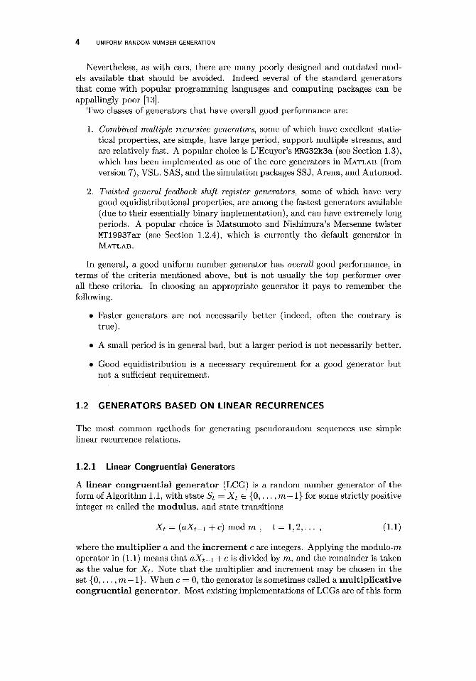
Nevertheless, as with cars, there are many poorly designed and outdated mod-els available that should be avoided. Indeed several of the standard generators that come with popular programming languages and computing packages can be appallingly poor [13].
Two classes of generators that have overall good performance are:
1. Combined multiple recursive generators, some of which have excellent statis-tical properties, are simple, have large period, support multiple streams, and are relatively fast. A popular choice is L'Ecuyer's MRG32k3a (see Section 1.3), which has been implemented as one of the core generators in MATLAB (from version 7), VSL, SAS, and the simulation packages SSJ, Arena, and Automod.
2. Twisted general feedback shift register generators, some of which have very good equidistributional properties, are among the fastest generators available (due to their essentially binary implementation), and can have extremely long periods. A popular choice is Matsumoto and Nishimura's Mersenne twister MT19937ar (see Section 1.2.4), which is currently the default generator in MATLAB.
In general, a good uniform number generator has overall good performance, in terms of the criteria mentioned above, but is not usually the top performer over all these criteria. In choosing an appropriate generator it pays to remember the following.
• Faster generators are not necessarily better (indeed, often the contrary is true).
• A small period is in general bad, but a larger period is not necessarily better.
• Good equidistribution is a necessary requirement for a good generator but not a sufficient requirement.
1.2 GENERATORS BASED ON LINEAR RECURRENCES
The most common methods for generating pseudorandom sequences use simple linear recurrence relations.
1.2.1 Linear Congruential Generators
A linear congruential generator (LCG) is a random number generator of the form of Algorithm 1.1, with state St = Xt G { 0 , . . . , m — 1} for some strictly positive integer m called the modulus , and state transitions
Xt = (aXt-i +c) mod m , ί = 1,2, . . . , (1.1)
where the multiplier a and the increment c are integers. Applying the modulo-m operator in (1.1) means that aXt~\ +c is divided by TO, and the remainder is taken as the value for Xt. Note that the multiplier and increment may be chosen in the set { 0 , . . . , TO — 1}. When c = 0, the generator is sometimes called a multipl icative congruential generator. Most existing implementations of LCGs are of this form
GENERATORS BASED ON LINEAR RECURRENCES 5
— in general the increment does not have a large impact on the quality of an LCG. The output function for an LCG is simply
■ EXAMPLE 1.1 (Minimal Standard LCG)
An often-cited LCG is that of Lewis, Goodman, and Miller [24], who proposed the choice a = 75 = 16807, c = 0, and m = 23 1 - 1 = 2147483647. This LCG passes many of the standard statistical tests and has been successfully used in many applications. For this reason it is sometimes viewed as the minimal standard LCG, against which other generators should be judged.
Although the generator has good properties, its period (231 — 2) and statistical properties no longer meet the requirements of modern Monte Carlo applications; see, for example, [20].
A comprehensive list of classical LCGs and their properties can be found on Karl Entacher's website:
http : / / r a n d o m . m a t . s b g . a c . a t / r e s u l t s / k a r l / s e r v e r /
The following recommendations for LCGs are reported in [20]:
• All LCGs with modulus 2P for some integer p are badly behaved and should not be used.
• All LCGs with modulus up to 26 1 « 2 x 10¹⁸ fail several tests and should be avoided.
1.2.2 Multiple-Recursive Generators
A multiple-recursive generator (MRG) of order A; is a random number gen-erator of the form of Algorithm 1.1, with state St = Xt = (Xt-k+i, ■ ■ ■ ,Xt)T £ { 0 , . . . , TO — l} f c for some modulus TO and state transitions defined by
Xt = (a^Xt-i H h akXt-k) mod m , t = k,k + l,..., (1.2)
where the multipliers {OJ,Z function is often taken as
The maximum period length for this generator is mk — 1, which is obtained if (a) TO is a prime number and (b) the polynomial p(z) — zk — Σί=ι a,iZk~l is primitive using modulo m arithmetic. Methods for testing primitivity can be found in [8, Pages 30 and 439]. To yield fast algorithms, all but a few of the {a{\ should be 0.
MRGs with very large periods can be implemented efficiently by combining sev-eral smaller-period MRGs (see Section 1.3).
1 , . . . , k} lie in the set { 0 , . . . , m — 1}. The output
Xt TO
6 UNIFORM RANDOM NUMBER GENERATION
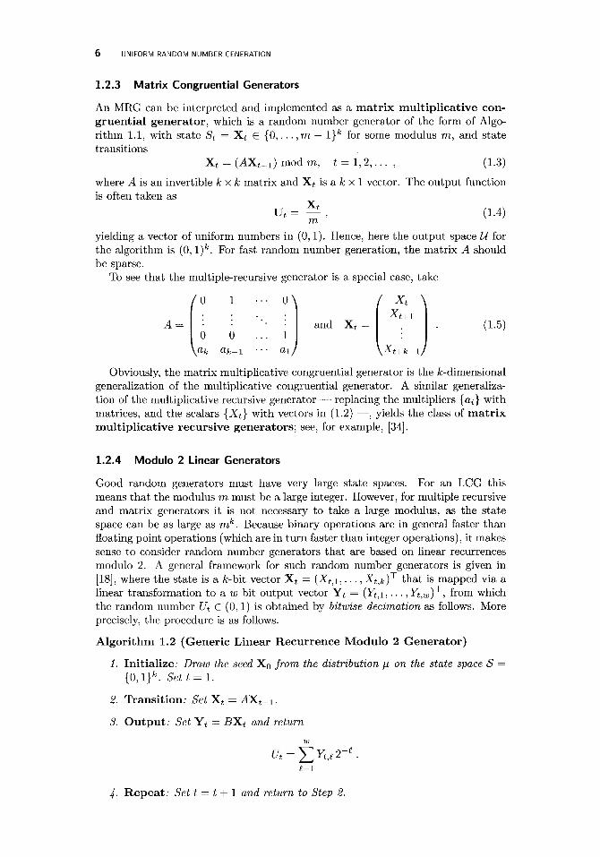
1.2.3 Matrix Congruential Generators
An MRG can be interpreted and implemented as a matr ix mult ipl icative con-gruential generator, which is a random number generator of the form of Algo-rithm 1.1, with state S t = X t € { 0 , . . . , m — l}k for some modulus m, and state transitions
X t = ( 4 X t _ i ) mod TO, ΐ = 1,2, . . . , (1.3)
where A is an invertible kxk matrix and Xt is a k x 1 vector. The output function is often taken as
U t = * i , (1.4) TO
yielding a vector of uniform numbers in (0,1). Hence, here the output space U for the algorithm is (0, l)k. For fast random number generation, the matrix A should be sparse.
To see that the multiple-recursive generator is a special case, take
A =
/ 0 1 ·
0 0 \flfc flfc-1 ·
·· o\
.. 1 ·· aij
and X t — ( Xt \ Xt+l
\Xt+k-lJ
(1.5)
Obviously, the matrix multiplicative congruential generator is the fc-dimensional generalization of the multiplicative congruential generator. A similar generaliza-tion of the multiplicative recursive generator — replacing the multipliers {<ij} with matrices, and the scalars {Xt} with vectors in (1.2) —, yields the class of matr ix multiplicative recursive generators; see, for example, [34].
1.2.4 Modulo 2 Linear Generators
Good random generators must have very large state spaces. For an LCG this means that the modulus TO must be a large integer. However, for multiple recursive and matrix generators it is not necessary to take a large modulus, as the state space can be as large as mk. Because binary operations are in general faster than floating point operations (which are in turn faster than integer operations), it makes sense to consider random number generators that are based on linear recurrences modulo 2. A general framework for such random number generators is given in [18], where the state is a fc-bit vector X t = {Xt,i, ■ ■ ■, Xt,k)T that is mapped via a linear transformation to a w-bit output vector Y t = (it . i i · · · , Yt,w)T, from which the random number Ut G (0,1) is obtained by bitwise decimation as follows. More precisely, the procedure is as follows.
Algor i thm 1.2 (Generic Linear Recurrence M o d u l o 2 Generator)
1. Initialize: Draw the seed Xo from the distribution μ on the state space S ■ {0, l} f c . Sett = l.
2. Transition; Set X t = A X t _ i .
3. Output : Set Y t = ßX E and return
w
4- Repea t : Set t = t + 1 and return to Step 2.
GENERATORS BASED ON LINEAR RECURRENCES 7
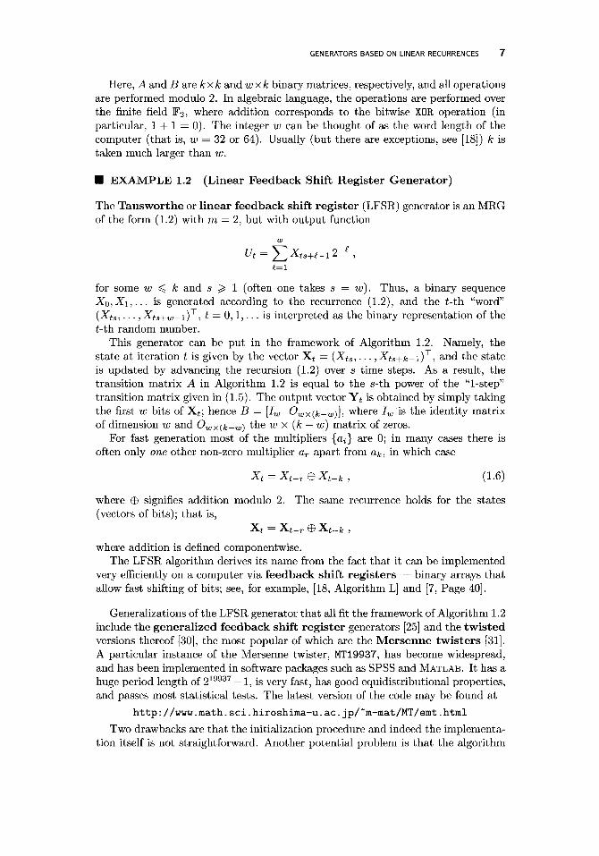
Here, A and B are kxk and wxk binary matrices, respectively, and all operations are performed modulo 2. In algebraic language, the operations are performed over the finite field F2, where addition corresponds to the bitwise XOR operation (in particular, 1 + 1 = 0). The integer w can be thought of as the word length of the computer (that is, w = 32 or 64). Usually (but there are exceptions, see [18]) k is taken much larger than w.
■ EXAMPLE 1.2 (Linear Feedback Shift Register Generator)
The Tausworthe or linear feedback shift register (LFSR) generator is an MRG of the form (1.2) with m = 2, but with output function
w
e=i
for some w ^ k and s ^ 1 (often one takes s = w). Thus, a binary sequence Χο,Χι,... is generated according to the recurrence (1.2), and the ί-th "word" {Xts, ■ ■ ■, Xts+w-i)T, t = 0 , 1 , . . . is interpreted as the binary representation of the ί-th random number.
This generator can be put in the framework of Algorithm 1.2. Namely, the state at iteration t is given by the vector X t = (Xts, ■ ■ ■, Xts+k-i)T, and the state is updated by advancing the recursion (1.2) over s time steps. As a result, the transition matrix A in Algorithm 1.2 is equal to the s-th power of the "1-step" transition matrix given in (1.5). The output vector Y t is obtained by simply taking the first w bits of X ( ; hence B = [Iw O œ x (£_„,)], where Iw is the identity matrix of dimension w and Owx^-w) the w x (k — w) matrix of zeros.
For fast generation most of the multipliers {ai} are 0; in many cases there is often only one other non-zero multiplier ar apart from α^, in which case
Xt = Xt-r Θ Xt-k , (1.6)
where ® signifies addition modulo 2. The same recurrence holds for the states (vectors of bits); that is,
X* = X t - r ® Xt-fc >
where addition is defined componentwise. The LFSR algorithm derives its name from the fact that it can be implemented
very efficiently on a computer via feedback shift registers — binary arrays that allow fast shifting of bits; see, for example, [18, Algorithm L] and [7, Page 40].
Generalizations of the LFSR generator that all fit the framework of Algorithm 1.2 include the generalized feedback shift register generators [25] and the twis ted versions thereof [30], the most popular of which are the Mersenne twisters [31]. A particular instance of the Mersenne twister, MT19937, has become widespread, and has been implemented in software packages such as SPSS and MATLAB. It has a huge period length of 2 1 9 9 3 7 — 1, is very fast, has good equidistributional properties, and passes most statistical tests. The latest version of the code may be found at
h t t p : / / w w w . m a t h . s e i . h i r o s h i m a - u . a c . j p/~m-mat/MT/emt.html
Two drawbacks are that the initialization procedure and indeed the implementa-tion itself is not straightforward. Another potential problem is that the algorithm
8 UNIFORM RANDOM NUMBER GENERATION
recovers too slowly from the states near zero. More precisely, after a state with very few Is is hit, it may take a long time (several hundred thousand steps) before getting back to some state with a more equal division between Os and Is. Some other weakness are discussed in [20, Page 23].
The development of good and fast modulo 2 generators is important, both from a practical and theoretical point of view, and is still an active area of research, not in the least because of the close connection to coding and cryptography. Some recent developments include the WELL (well-equidistributed long-period linear) generators by Panneton et al. [35], which correct some weaknesses in MT19937, and the SIMD-oriented fast Mersenne twister [38], which is significantly faster than the standard Mersenne twister, has better equidistribution properties, and recovers faster from states with many 0s.
1.3 COMBINED GENERATORS
A significant leap forward in the development of random number generators was made with the introduction of combined generators. Here the output of several generators, which individually may be of poor quality, is combined, for example by shuffling, adding, and/or selecting, to make a superior quality generator.
■ EXAMPLE 1.3 (Wichman-Hi l l )
One of the earliest combined generators is the Wichman-Hill generator [41], which combines three LCGs:
Xt = (171 Xt_x) mod mi (mi = 30269) ,
Yt = (172 Yt_i ) mod m 2 (m2 = 30307) ,
Zt = (170 Z t _i ) mod m 3 (m3 = 30323) .
These random integers are then combined into a single random number
TT Xt , Yt , Zt , Ut = 1 1 mod 1 .
mi m 2 ™3
The period of the sequence of triples (Xt,Yt, Zt) is shown [42] to be (mi — l ) (m 2 — l)("T-3 — l ) / 4 ~ 6.95 x 10¹², which is much larger than the individual periods. Zeisel [43] shows that the generator is in fact equivalent (produces the same output) as a multiplicative congruential generator with modulus m = 27817185604309 and multiplier a = 16555425264690.
The Wichman-Hill algorithm performs quite well in simple statistical tests, but since its period is not sufficiently large, it fails various of the more sophisticated tests, and is no longer suitable for high-performance Monte Carlo applications.
One class of combined generators that has been extensively studied is that of the combined multiple-recursive generators, where a small number of MRGs are combined. This class of generators can be analyzed theoretically in the same way as single MRG: under appropriate initialization the output stream of random numbers of a combined MRG is exactly the same as that of some larger-period