In the literature on quantum computation, quantum logic means an algebra of the qubits and quantum gates of a quantum computer, [Berman et al. , 2005; Bouwmeester et al. , 2000; Fiorentino and Wong, 2004; Franson et al., 2002; Nielsen and Chuang, 2000; Pavicic, 2005; Shapiro et al. , 2003; Zurek and Laflamme, 1996] . This quantum logic of qubits (also called quantum computational logic [Cattaneo et al. , 2004; Gudder, 20031) is a formalism of finite tensor products of two-dimensional Hilbert spaces and will not be the subject matter of the present chapter.
Here we deal with a quantum logic defined as an algebra related to a complete description of quantum systems and its role in quantum computation. A complete description of a quantum system, say a molecule, includes not only spins - as with qubits - but also positions, momenta, and potentials of nucleons and electrons, and this, in the standard approach, requires infinite-dimensional Hilbert spaces. In the second half of the 20th century, numerous attempts to reduce the latter Hilbert space formalism to various types of algebras have been put forward [Holland, 1995]. The main idea behind these attempts was to relate Hilbert space observables directly to experimental setups and results [Jauch, 1968; Ludwig, 1985; Ludwig, 1987; Piron, 1976].
The latter idea has not come true, but mathematically the project has been a success. In particular, the Hilbert lattice has been proved isomorphic to the set of subspaces of an infinite-dimensional Hilbert space. So, in an attempt to treat general quantum systems with the help of a quantum computer, we might venture to introduce such an algebraic description of the systems directly into it. However, as with classical problems, we have to translate a description of quantum systems into a language a quantum computer would understand. To make this point, before we dwell on quantum systems, we shall briefly review how we can make such a translation for a classical problem to be computed on a quantum computer.
One of the most successful quantum computing algorithms so far is Shor's algorithm for the classical problem of factoring numbers [Shor, 1997] . Factoring numbers with classical algorithms on classical computers is conjectured to be a problem of exponential complexity with respect to the number of bits. To verify (by the brute force approach) whether x, y > 1 exist such that xy = N, we have
756 Mladen Pavici!: and Norman D. Megill
to check all possible x's starting with x = 2 and ending (in the most unfavourable case) with x = ..[N. The number of checks obviously does not rise exponentially with N. When we say that the time needed to carry out the checking rises exponentially, we mean with respect to the number of bits n required to handle the divisions within a digital computer, where N � 2" [Pavicic, 2005] .
The way of handling operations in a computer is what differentiates a classical from a quantum computer and what enables the latter one to speed up exponentially given computations. To see this let us look at the all-optical "calculator" shown in Fig. 1 proposed by Johann Summhammer [Summhammer, 1997] .
Figure 1. Physical calculation by means of a Mach-Zehnder interferometer. When the phase difference <Po - <P1 is equal to an integer multiplier of 7r, the photon ideally will never end up in detector Do . BS are 50:50 beam splitters.
Photons enter the Mach-Zehnder interferometer one by one and interfere depending on the phase difference <Po - <P1 imposed by the phase shifters shown in the figure. The probability of detector D1 registering a photon is
2 <P1 - <Po p = cos 2 . (1)
Hence, when the phase difference <Po - <P1 is equal to an integer multiplier of 7r, we have p = 1, Le. , a constructive interference at the lower exit and a destructive one at the upper one. In other words, ideally, detector D1 will always click and detector Do will never click.
To factor a number N, let us increase the phase shift in discrete steps 27r j k so as to have <Po - <P1 = 27rN jk. Until we arrive at an integer k which factors N, we will always have some clicks in Do. Our qubit - photon state - will be in a superposition that is not completely destructive with respect to the upper exit. By repeating each step many times, say N times, we will altogether need - in order to reach and confirm a completely destructive interference with respect to the upper exit - to carry out N..[N checks, to make sure that the response of Do is negligible when we reach a k for which Nj k is an integer and p given by Eq. (1) equals 1 .
Quantum Logic and Quantum Computation 757
We see that the way of introducing and dividing numbers into this physical computer is essentially different from the one we use with digital computers. In a classical computer, the bigger the numbers are, the more bits and therefore more transistors we have to employ for handling their factorization. The number of transistors and gates required to handle each division grows polynomially with the number of bits n.
In a Mach-Zehnder interferometer, we carry out each division by picking a particular phase difference. So, it is always just one phase difference, irrespective of the size of the number. 1 If we take the photon within the interferometer to be a quantum bit, in quantum computation parlance called qubit, and the MachZehnder interferometer to be a quantum logic gate, or simply a quantum gate, we obtain a single gate acting as a single computing unit, providing us with the desired result within a single step. We denote the state of a photon exiting from the lower sides of the Mach-Zehnder beam splitters by II} and one exiting from their upper sides by 10} . The qubit (photon) can be in any of infinitely many superpositions a lO} + ,BIl} within the interferometer, one of which provides us with a definite result with the probability equal to l.
Now, what enables an exponential speedup of the quantum factoring tasks is an algorithm - Shor's algorithm - that makes use of a superposition of qubit states so as to reduce the problem of searching for factors to searching for a period of the wave function representing the superposition. When applied, it reduces the required number of checks to one polynomial in 10g(N) [ittenger, 1999]. This algorithm as well as all other known quantum algorithms are based on Fourier transforms, and the main additional feature of quantum gates is that they can perform Fourier transforms. The next feature we require is scalability, so that adding new gates preserves the achieved speedup while increasing the computational power. Linear optics elements - the Mach-Zehnder interferometer being one of them - can be integrated into a scalable all-optical quantum computer [Browne and Rudolph, 2005; Ralph et al. , 2005] . Similar scaling up can be achieved with ion, quantum-dot, QED, and Kane quantum computers by using recent hardware and software blueprints, at least in principle [Pavicic, 2005]. At present, quantum computation relies on the way we introduce and encode the input data into states of qubits within a quantum computer as well as on the algorithms we apply on the states. There are still only a few such algorithms, but for various classical problems we shall most probably arrive at new applications gradually, as was the case with classical computation (it took half a century to reach a digital implementation of 3D animation and voice recognition, for example) .
There is, however, an application that seems to be radically different from all the others, and this is the quantum computation and simulation of quantum systems. Classically, we compute the properties of an atom or molecule by solving a Schro.. dinger equation with the help of sophisticated algorithms for approximating and
10f course, up to a realistic limit of the interferometer - it cannot discern phases that correspond to numbers bigger than 1010, but it can be integrated together with other linear optics elements into an all-optical quantum computer.
758 Mladen PaviCic and Norman D. Megill
solving the equation, all of which are of exponential complexity with respect to the number of observables. For a quantum computer, several algorithms for solving a Schrodinger equation that provide an exponential speed increase with respect to classical computers have been proposed [Abrams and Lloyd, 1999; Boghosian and Taylor, 1998; Gramss, 1998; Zalka, 1998] . They start with rather simple wave functions, discretize them, and then introduce them into the Schrodinger equation, which then reduces to an eigenvalue problem that can be solved in a Fourier transform approach analogous to the one we used to factor numbers. In the case of more general Schrodinger equations, though, we no longer have an obvious and straightforward algorithm - no algorithms are known that implement Fourier transforms for simulating and determining the evolution of general arbitrary quantum systems.
However, if we found a quantum algebra for describing quantum systems, such as atoms and molecules, which a quantum computer could "read" directly, then it would instantly simulate the systems, tremendously speeding up its "calculation," i.e. , obtaining information on its behaviour. No special algorithm would be needed. We could think of simulating existing and still non-existing molecules under chosen conditions. How can we achieve such a simulation?
When we talk about quantum systems and its theoretical Hilbert space, we know that there is a Hilbert lattice that is isomorphic to the set of subspaces of a particular infinite-dimensional Hilbert space and that we can establish a correspondence between elements of the lattice and solutions of a Schrodinger equation that corresponds to such a Hilbert space. But there is an essential problem here. Any Hilbert lattice is a structure based on first-order predicate calculus, and we simply cannot have a constructive procedure to introduce statements like there is or for all into a computer. Unlike with the Mach-Zehnder computer above, we do not have a recipe for introducing states of an arbitrary quantum system into a quantum computer.
What we might do, instead, is find classes of polynomial lattice equations that can serve in place of quantified statements. And in this chapter we are going to review how far we have advanced down this road, following [Megill and Pavicic, 2000] and [Pavicic, 2005] . If we can eventually establish a correspondence between such equations and solutions of the SchrOdinger equation, i.e., general wave functions, then we should be able to reduce any quantum problem to a polynomially complex eigenvalue problem. Whether the project can be carried out successfully awaits future developments, but this is the case with all projects in quantum computing.
In the next section, we deal with quantum logic defined as a Hilbert lattice. Quantum logic so defined is only one of the possible models of quantum logics considered in our chapter in Volume 1 [Pavicic and Megill, 2006] . In Section 3 we present the Greechie diagrams, in Section 4 generalized orthoarguesian equations and in Sections 5, 6, and 7 Godowski, Mayet-Godowski, and Mayet's E-equations, respectively. We end the chapter with a conclusion and open problems.
Quantum Logic and Quantum Computation 759
2 HILBERT LATTICE
A Hilbert lattice is a special kind of an orthomodular lattice, OML, which we introduced and defined in Definition 2.6 in our chapter in Volume 1 [Pavicic and Megill, 2006] . The axioms added to an OML to make it represent Hilbert space are (as one example of several slightly different axiomatizations) the following ones [Beltrametti and Cassinelli, 1981; Kalmbach, 1986] . DEFINITION 1. 2 An orthomodular lattice which satisfies the following conditions is a Hilbert lattice, 'H£.
1 . Completeness: The meet and join of any subset of an 'HC exist.
2. Atomicity: Every non-zero element in an 'HL is greater than or equal to an atom. (An atom a is a non-zero lattice element with 0 < b :s a only if b = a.)
3. Superposition principle: (The atom c is a superposition of the atoms a and b if c i= a, c i= b, and c :s a U b.) (a) Given two different atoms a and b, there is at least one other atom c,
c i= a and c i= b, that is a superposition of a and b. (b) If the atom c is a superposition of distinct atoms a and b, then atom a
is a superposition of atoms b and c. 4. Minimal length: The lattice contains at least three elements a, b, c satisfying:
O < a < b < c < 1 .
These conditions imply an infinite number of atoms in 'HL as shown by Ivert and SjOdin [Ivert and SjOdin, 1978] .
One can prove the following theorem [Mackey, 1963; MacLaren, 1964; Varadarajan, 1968] . THEOREM 2. For every Hilbert lattice 'HC there exists a field JC and a Hilbert space 'H over JC such that the set of closed subspaces of the Hilbert space, C('H) is ortho-isomorphic to 'HL.
Conversely, let 'H be an infinite-dimensional Hilbert space over a field JC and let
C('H) �f {X � 'H I X_LL = X} (2)
be the set of all closed subspaces of 'H. Then C('H) is a Hilbert lattice relative to:
and (3)
In order to determine the field over which the Hilbert space in Theorem 2 is defined, we make use of the following theorem proved by Maria Pia Soler [Soler, 2995; Holland, 1995].
2For additional definitions of the terms used in this section see Refs. [Beltrametti and Cassinelli, 1981; Holland, 1995; Kalmbach, 1986] .
760 Mladen Pavicic and Norman D. Megill
THEOREM 3. The Hilbert space 'It from Theorem 2 is an infinite-dimensional Hilbert space defined over a real, complex, or quaternion {skew} field if the following condition is met:
• Infinite orthonormality: 'ltL contains a countably infinite sequence of orthonormal elements.
Thus we do arrive at a full Hilbert space, but the axioms for the Hilbert lattices that we used for this purpose are rather involved. This is because in the past, the axioms were simply read off from the Hilbert space structure and were formulated as quantified statements of the first order that cannot be implemented into a quantum computer.
3 GREECHIE DIAGRAMS
The Hilbert lattice equations that we will be describing in subsequent sections will require some method for proving that they are independent from the equations for OMLs. This will show that these equations indeed extend the equational theory for Hilbert lattices beyond that provided by just the OML equations. We will usually show the independence by exhibiting finite OMLs in which the new Hilbert lattice equations fail. Typically, these counterexample OMLs are very large lattices with dozens of nodes, and it is inconvenient to represent them with standard lattice (Hasse) diagrams. Instead, we will use a much more compact method for representing OMLs called Greechie diagrams. Because of their importance as a tool, we will describe them in some detail in this section.
The following definitions and theorem we take over from Kalmbach [Kalmbach, 1983] and Svozil and Tkadlec [Svozil and Tkadlec, 1996]. Definitions in the framework of quantum logics (IT-orthomodular posets) the reader can find in the book of Ptak and Pulmannova [Ptak and Pulmannova, 1991] .
DEFINITION 4. A diagram is a pair (V, E), where V i= 0 is a set of atoms (drawn as points) and E � exp V \ {0} is a set of blocks (drawn as line segments connecting corresponding points). A loop of order n 2: 2 (n being a natural number) in a diagram (V, E) is a sequence (el , . . . eb) E en of mutually different blocks such that there are mutually distinct atoms Vl , . . . , Vn with Vi E einei+l (i = 1, . . . , n, en+l = el ) . DEFINITION 5. A Greechie diagram is a diagram satisfying the following conditions:
(1) Every atom belongs to at least one block.
(2) If there are at least two atoms then every block is at least 2-element.
(3) Every block which intersects with another block is at least 3-element.
(4) Every pair of different blocks intersects in at most one atom.
Quantum Logic and Quantum Computation 761
(5) There is no loop of order 3.
THEOREM 6. For every Greechie diagram with only finite blocks there is exactly one (up to an isomorphism) orthomodular poset such that there are one-to-one correspondences between atoms and atoms and between blocks and blocks that preserve incidence relations. The poset is a lattice if and only if the Greechie diagram has no loops of order 4.
In general, Greechie diagrams correspond to Boolean algebras "pasted" together. First we will show examples of individual blocks in order to illustrate how they correspond to Boolean algebras. Then we will introduce the concepts needed to understand how Boolean algebras can be interconnected to represent more general OMLs.
The Hasse and Greechie diagrams for the Boolean algebras corresponding to 2-, 3-, and 4-atom blocks are shown in Fig. 2. The Greechie diagram for a given lattice may be drawn in several equivalent ways: Fig. 3 shows the same Greechie diagram drawn in two different ways, along with the corresponding Hasse diagram. From the definitions we see that the ordering of the atoms on a block does not matter, and we may also draw blocks using arcs as well as straight lines as long as the blocks remain clearly distinguishable.
x
x •
1
o X'
•
X'
X' x
x •
1
o y •
z •
Zl
z
w •
x •
1
o y •
z •
Figure 2. Greechie diagrams for Boolean lattices 22, 23, and 2\ labelled with the atoms of their corresponding Hasse diagrams shown above them. (24 was adapted from [Beran, 1985, Fig. 18, p. 84] .)
Recall that a poset (partially ordered set) is a set with an associated ordering relation that is reflexive (a :5 a), antisymmetric (a :5 b, b :5 a imply a = b), and transitive (a :5 b, b :5 c imply a :5 c) . An orthoposet is a poset with lower and
762 Mladen PaviCic and Norman D. Megill
upper bounds 0 and 1 and an operation ' satisfying (i) if a :5 b then b' :5 a'; (ii) a" = a; and (iii) the infimum a n a' and the supremum a U a' exist and are 0 and 1 respectively. A lattice is a poset in which any two elements have an infimum and a supremum. An orthoposet is orthomodular if a :5 b implies (i) the supremum a U b' exists and (ii) a U (a' n b) = b. A lattice is orthomodular if it is also an orthomodular poset. For example, Boolean algebras such as those of Fig. 2 are orthomodular lattices. A u-orthomodular poset is an orthomodular poset in which every countable subset of elements has a supremum. An atom of an orthoposet is an element a i= 0 such that b < a implies b = O.
v � / z w V y x
x
T
1
v' Z' v Z
o Figure 3. Two different ways of drawing the same Greechie diagram, and its corresponding Hasse diagram.
In the literature, there are several different definitions of a Greechie diagram. For example, Beran [Beran, 1985, p. 144] forbids 2-atom blocks. Kalmbach [Kalmbach, 1983, p. 42] as well as Ptak and Pulmannova [Ptak and Pulmannova, 1991, p. 32] include all diagrams with 2-atom blocks connected to other blocks as long as the resulting pasting corresponds to an orthoposet. However, the case of 2-atom blocks connected to other blocks is somewhat complicated; for example, the definition of a loop in Definition 4 must be modified (e.g. [Kalmbach, 1983, p. 42]) and no longer corresponds to the simple geometry of a drawing of the diagram. The definition of a Greechie diagram also becomes more complicated; for example a pentagon (or any n-gon with an odd number of sides) made out of 2-atom blocks is not a Greechie diagram (Le. does not correspond to any orthoposet) .
The definition of Svozil and Tkadlec [Svozil and Tkadlec, 1996] that we adopt, Definition 5, excludes 2-atom blocks connected to other blocks. It turns out that all orthomodular posets representable by Kalmbach's definition can be represented with the diagrams allowed by Svozil and Tkadlec's definition. But the latter definition eliminates the special treatment of 2-atom blocks connected to other blocks and in particular simplifies any computer program designed to process Greechie diagrams.
Svozil and Tkadlec's definition further restricts Greechie diagrams to those diagrams representing orthoposets that are orthomodular by forbidding loops of order less than 4, unlike the definitions of Beran and Kalmbach. The advantage appears to be mainly for convenience, as we obtain only those Greechie diagrams that cor-
Quantum Logic and Quantum Computation 763
respond to what are sometimes called "quantum logics" (IT-orthomodular posets) . (We note that the term "quantum logic" is also used to denote a propositional calculus based on orthomodular or weakly orthomodular lattices [Pavicic and Megill, 1999]).
The definition allows for Greechie diagrams whose blocks are not connected. In Fig. 4 we show the Greechie diagram for the Chinese lantern M02 using unconnected 2-atom blocks. This example also illustrates that even when the blocks are unconnected, the properties of the resulting orthoposet are not just a simple combination of the properties of their components (as one might naIvely suppose), because we are adding disjoint sets of incomparable nodes to the orthoposet. As is well-known ( [Kalmbach, 1983, p. 16]), M02 is not distributive, unlike the Boolean blocks it is built from.
1
x' x Y y' �-- - - - - - -� x' y'
(a)
0 Figure 4. Greechie diagram for the lattice M02 and its Hasse diagram. The dashed line indicates that the unconnected blocks belong to the same Greechie diagram.
4 GEOMETRY: GENERALIZED ORTHOARGUESIAN EQUATIONS
Before 1975, the orthomodular lattice (OML) equations were the only ones that were known to hold in a Hilbert lattice. These have been extensively studied in a vast body of research papers and books, particularly in the context of the logic of quantum mechanics, and so "orthomodular lattice" and "quantum logic" have become almost synonymous.
In 1975, Alan Day discovered an equation that holds in any Hilbert lattice but does not in all OMLs [Greechie, 19811 . He derived the equation, called the orthoarguesian law, by imposing weakening orthogonality hypotheses on the socalled Arguesian law, an equation closely related to the famous law of projective geometry discovered by Desargues in the 1600's.3
In 2000, Megill and Pavicic discovered a new infinite class of equations that hold in any Hilbert lattice,4 called generalized orthoarguesian equations or nOA laws, n = 3, 4, . . . < 00, a special case of which is the orthoarguesian law for n = 4.
3as part of an effort to help artists, stonecutters, and engineers 4and therefore in any infinite-dimensional Hilbert space
764 Mladen Pavicic and Norman D. Megill
We recall the following definitions for reference here and later: a � b �f a' U (a n b) and and a = b �f (a n b) u (a' n b') .
DEFINITION 7 . We define an operation <;;} on n variables al , . ' " an (n 2: 3) as follows:5
THEOREM 8. The nOA laws
(6)
hold in any Hilbert lattice.
Proof. To show that the nOA laws hold in C(1t), Le., in a Hilbert lattice, we closely follow the proof of the orthoarguesian equation (40A in our notation) in Ref. [Greechie, 1981] . We recall that in lattice C(1t), the meet corresponds to set intersection and ::; to �. We replace the join with subspace sum + throughout: the orthogonality hypotheses permit us to do this on the left-hand side of the conclusion [Kalmbach, 1983, Lemma 3 on p. 67], and on the right-hand side we use a+b � a U b.
as: In Ref. [Megill and Pavicic, 2000] we have shown that Eq. (6) can be written
ao ..1 bo & al ..l bl & & an-2 ..l bn-2 ::::}
(ao U bo) n (al U bl ) n . . . n (an-2 U bn-2) ::; bo U (ao n (al U ( . . . (ai U aj) n (bi U bj) . . . ))) , (7)
where a ..1 b �f a ::; b', n 2: 3, and 0 ::; i, j ::; n - 2. (The construction of the righthand portion in ellipses can be inferred starting from the 30A basis, described in the next paragraph, and building it up from n to n + 1 with the replacements described in the last two sentences of this proof.)
The proof is by induction on n, starting at n = 3. Suppose x is a vector belonging to the left-hand side of (7) . Then there exist vectors Xo E ao, Yo E bo, . . . , Xn-2 E an-2, Yn-2 E bn-2 such that x = Xo + Yo = . . . = Xn-2 + Yn-2 ' Hence Xk -XI = YI -Yk for 0 ::; k, l ::; n-2. In Eq. (7) we assume, for our induction
5.... b . (n) b ' . h (n-l) b . nl th tw I" t . bl I . .LO 0 tam == we su stItute In eac == su expressIOn 0 y e o exp leI varIa es, eavmg
the other variables the same. For example, (a2 Wa5) on the right side of (5) for n = 5 means (� �) (� (a2 == a5) U «a2 == a4) n (a5 ==a4» which means (((a2 -+ a3) n (a5 -+ a3» U «a� -+ a3) n (a� -+ a3» )U««a2 -+ a3) n (a4 -+ a3» U«a� -+ a3) n (a4 -+ a3» ) n (((a5 -+ a3)n (a4 -+ a3» U«a� -+ a3) n (a4 -+ a3» » .
Quantum Logic and Quantum Computation 765
hypothesis, that the components of vector x = Xo + Yo can be distributed over the leftmost terms on the right-hand side of the conclusion as follows:
v Xl + (Xo - Xl) = Xo
v Yo + Xo = X
In particular, if we discard the right-hand ellipses, we obtain a C(1t) proof of the 30A law; this is the basis for our induction.
Let us first extend Eq. (7) by adding variables an-l and bn-l to the hypotheses and left-hand side of the conclusion. The extended Eq. (7) so obtained obviously continues to hold in C(1t) . Suppose X is a vector belonging to the left-hand side of this extended Eq. (7) . Then there exist vectors Xo E ao, Yo E bo , . . . , Xn-l E an-l , Yn-l E bn-l such that X = Xo + Yo = . . . = Xn-l + Yn-l . Hence Xk - XI = YI - Yk for 0 :5 k, l :5 n - 1. On the right-hand side of the extended Eq. (7), for any arbitrary sub expression of the form (ai U aj) n (bi U bj) , where i, j < n - 1, the vector components will be distributed (possibly with signs reversed) as Xi - Xj E ai+aj and Xi - Xj = -Yi + Yj E bi+bj . If we replace (ai U aj) n (bi U bj) with (ai U aj ) n (bi U bj) n (((ai U an-l) n (bi U bn-l)) U ( (aj U an-l) n (bj U bn-l))) , components Xi and Xj can be distributed as
(ai+aj) n (bi+bj) n (( (ai+an-l) n (bi+bn-l) )+( (aj+an-l ) n (bj+bn-l))) "'-v-" '-v-' � � � "-v-' Xi - Xj = -Yi + Yj Xi - Xn-l = -Yi + Yn-l -Xj + Xn-l = Yj - Yn-l
." (Xi - Xn-l) + (-Xj + Xn-l) = Xi - Xj
so that Xi - Xj remains an element of the replacement subexpression. We continue to replace all sub expressions of the form (ai U aj) n (bi U bj) , where i, j < n - 1, as above until they are exhausted, obtaining the (n + 1 )OA law:
ao ..1 bo & al ..l bl & & an-l ..l bn-l �
(ao U bo) n (al U bl) n . . . n (an-l U bn-l) :5 bo U (ao n (al U ( . . . (ai U aj) n (bi U bj))
n(((ai U an-l) n (bi U bn-l) ) U ((aj U an-l) n (bj U bn-l ))) · · · ))) . (8)
• COROLLARY 9. In any OML, Day's orthoarguesian law [Greechie, 1981] is equivalent to the 40A law and the equations found by Godowski and Greechie in 1984 [Godowski and Greechie, 1984] are equivalent to each other and to 30A.
Proof. As given in Ref. [Megill and Pavicic, 2000] . •
766 Mladen PaviCic and Norman D. Megill
THEOREM 10. Any ortholattice (OL) [PaviCic and Megill, 2006, Def. I] in which an nOA law holds is orthomodular. No nOA law holds in all OMLs.
Proof. All nOA laws fail in ortholattice 06 (benzene ring, hexagon) [Pavicic and Megill, 2006, Sec. 2] .
We prove the second statement of the theorem by finding an orthomodular lattice in which the 30A law fails. In Figure 5 we show the smallest such Greechie diagram, containing 13 atoms. Since the (n + l)OA law implies the nOA law (see Theorem 11 below), the result follows. •
We conjecture that the second statement of the following theorem holds for any n. To prove it for n 2: 6 is an open problem.
THEOREM 11. In an OL, the nOA law implies the (n - l)OA law for any n > 3. In an OL, the nOA law does not imply the (n + l)OA law for 3 :5 n :5 5.
Proof. The first statement easily follows from the definition of the nOA laws. As for the second statement, we have three cases. For n = 3, the 30A law holds
in the 17-10-oa3p4f given in Fig. 5 and the 40A law fails. For n = 4, the 40A law holds in 22-13-oa4p5f given in the same figure, but the 50A law fails.6
Figure 5. The smallest Greechie diagram in which the OML law holds and the 30A law fails, the 30A law holds and the 40A fails, and the two smallest Greechie diagrams in which 40A holds and 50A fails. Cf. Figs. 8 b and 9 of [Megill and Pavici<�, 2000] . McKay, Megill, and Pavici<� also introduced a textual way of writing down Greechie diagrams that is self-explanatory for 13-7-0MLp-oa3f in the figure: 123 , 345 , 567 , 789 , 9AB , BC1 , BD5.
For n = 5, the 50A law holds in 28-18-oa5p6f (Fig. 6) but the 60A law fails. These counterexamples were found using a program written by Brendan McKay
that exhaustively generates finite OML lattices, that in turn fed a program written by Norman Megill that tests the nOA laws against those lattices [McKay et al. , 2000] . The nOA laws are very long equations whose lengths grow exponentially
6The notation "35-23-oa5p6r' means "35 atoms, 23 edges, in which the 50A law passes and the 60A law fails."
Quantum Logic and Quantum Computation 767
28-18-oaSp6f-a 28-18-oa5p6f-b 35-23-oaSp6f
Figure 6. Three lattices in which the 50A law holds and the 60A fails. The 28 atom ones are apparently examples of the smallest such lattices. The 35 atom one is from a set of lattices we conjecture to contain the smallest lattices in which the 60A law holds and the 70A fails. (Bigger dots denote the vertices of the polygon.)
with n (with 4 · 3n-2 + 3 variable occurrences when expanded to elementary operations). As n increases, the difficulty of finding these counterexamples increases exponentially. Finding counterexamples required over 10 years of CPU time on the Cluster Isabella (224 CPUs) and Civil Enginering Cluster (60 CPUs) of the University of Zagreb. Some additional lattices in which 50A holds and 60A fails are:
that, while weaker than the nOA laws (verified to be strictly weaker for n = 3, 4), nonetheless cannot be derived from the OML axioms [Megill and Pavicic, 2000] .
The nOA identity laws bear a resemblance to the OML law in the form a = b = 1 {:} a = b. Thus is it natural to think that they might be equivalent to the nOA laws. This is known as the orthoarguesian identity conjecture, which asks whether the nOA laws can be derived, in an OML, from Eq. (9). Tests run against several million finite lattices (for n = 3) have not found a counterexample, but the conjecture has so far defied attempts to find a proof.
An affirmative answer to this conjecture would provide us with a powerful tool to prove new equivalents to the nOA laws. It turns out that it is often much easier to derive the nOA identity law from a conjectured nOA law equivalent than it is to derive the nOA law itself. For example, under the assumption that the 30A identity law implies the 30A law, all of the following conditions would be established as equivalents to the 30A law (where aGb means a = (a U b) n (a U b') i.e. a commutes with b) :
(3) (al � a3) n (al =a2) (3) (al � a3) n (al =a2)
( I )' ( (3) ) al � a3 n al =a2 ( I )' ( (3) ) al � a3 n al = a2 ( I )' ( (3) ) al � a3 n al =a2
(3) a3 n (al � a3) n (al =a2) (3) a3 n (al � a3) n (al =a2) (3) a3 n (al � a3) n (al =a2)
(3) ((al � a3) n (al = a2)) � a3 (3) ((al � a3) n (al = a2)) � a3
At the present time, only Eqs. (11) and (19) from the above set of conditions are known to be equivalent to the 30A law. Denoting the 30A law [Eq. (6) for n = 3]
Quantum Logic and Quantum Computation 769
and the 30A identity law [Eq. (9)1 by OA3 and 0I3 respectively, the currently known relationships among the above conditions are as follows. (Note that � means "the right-hand equation can be proved from the axiom system of OML + the left-hand equation added as an axiom.")
As we explained in Section 2, there is a way to obtain complex infinite-dimensional Hilbert space from the Hilbert lattice equipped with several additional conditions and without invoking the notion of state at all. States then follow by Gleason's theorem (see Theorem 41 in Section 8) . However, we can also define states directly on an ortholattice, and then it turns out that such a definition generates many properties of the lattice that hold in any Hilbert lattice. In particular, the states generate the Godowski and Mayet-Godowski equations (on which we will elaborate in the next section) .
DEFINITION 13. A state (also called probability measures or simply probabilities [Kalmbach, 1998; Kalmbach, 1983; Kalmbach, 1986; Kalmbach, 1998; Ml}Czynski, 19721) on a lattice C is a function m : C ---+ [0, 11 such that m(l) = 1 and a ..1 b � m(a U b) = m(a) + m(b), where a ..l b means a :5 b' . LEMMA 14. The following properties hold for any state m:
DEFINITION 15. A nonempty set S of states on C is called a strong set of classical states if
(3m E S)(Va, b E C) ((m(a) = 1 � m(b) = 1) � a :5 b) (26)
and a strong set of quantum states if
(Va, b E L) (3m E S)((m(a) = 1 � m(b) = 1) � a :5 b) . (27)
We want to emphasize the difference between quantum and classical states . A classical state is the same for all lattice elements, while a quantum state might
770 Mladen PaviCic and Norman D. Megill
be different for each of the elements. The following theorem [Megill and Pavich;, 2000] shows us that a classical state can be be very strong.
THEOREM 16. Any ortholattice that admits a strong set of classical states is distributive.
In 1981, Radoslaw Godowski [Godowski, 1981] found an infinite series of equations partly corresponding to the strong set of quantum states given by Eq. (27), forming a series of algebras contained in the class of all orthomodular lattices and containing the class of all Hilbert lattices. Importantly, there are OMLs that do not admit a strong set of states, so Godowski's equations provide us with new equational laws that extend the OML laws that hold in Hilbert lattices.
Before deriving the equations themselves, we will first prove, directly in Hilbert space, that Hilbert lattices admit strong sets of states. This will provide some insight into how these equations arise.
THEOREM 17. Any Hilbert lattice admits a strong set of states.
Proof. We need only to use pure states defined by unit vectors: If a and b are closed subs paces of a Hilbert space 'It such that a is not contained in b, there is a unit vector u of 'It belonging to a - b. If for each c in the lattice of all closed subspaces of 'It, C('It), we define m(c) as the square of the norm of the projection of u onto c, then m is a state on 'It such that m(a) = 1 and m(b) < 1. This proves that C ('It) admits a strong set of states, and this proof works in each of the 3 cases where the underlying field is the field of real numbers, of complex numbers, or of quaternions.
We can formalize the proof as follows:
(Va, b E L) ((", a � b) => (3m E S) (m(a) = 1 & '" m(b) = 1)) => (Va, b E L) (3m E S)((m(a) = 1 => m(b) = 1) => a � b)
• We will now define the family of equations found by Godowski, introducing
a special notation for them. Then we will prove that they hold in any lattice admitting a strong set of states and thus, in particular, any Hilbert lattice.
DEFINITION 18. Let us call the following expression the Godowski identity:
al�an �f(al � a2) n (a2 � a3) n . . . n (an-l � an) n (an � al) , n = 3, 4, . . . (28)
We define an�al in the same way with variables ai and an-Hl swapped; in general ai�aj will be an expression with Ii - i l + 1 2: 3 variables ai, . . . , aj first appearing in that order. For completeness and later use (Theorem 24) we define
'Y def( ) 'Y def( ) ) ai=Ui = ai � ai = 1 and ai=ai+l = ai � ai+l n (ai+l � Ui = ai = ai+l , the last equality holding in any OML.
hold in all ortholattices, OL 's, with strong sets of states. An OL to which these equations are added is a variety smaller than OML.
We shall call these equations n-Go (3-Go, 4-Go, etc.) . We also denote by nGO (3GO, 4GO, etc.) the OL variety determined by n-Go and call it the nGO law.
Proof. By Definition 13 we have m(al � a2) = m(aD + m(al n a2) etc. , because a� :5 (a� U �), i.e. , a� ..1 (al n a2) in any ortholattice. Assuming m(al�an) = 1, we have m(al � a2) = . . . = m(an-2 � an) = m(an � al ) = 1. Hence, n = m(al � a2)+ · · · +m(an-2 � Un) +m(an � al ) = m(an � an-2) + · · · +m(a2 � al ) + m(al � an) . This last equality follows from breaking up, rearranging, and recombining the m(ai � aj) terms as described by the first sentence. Therefore, m(an � Un-2) = . . . = m(a2 � al ) = m(al � an) = 1. Thus, by Definition 15 for strong quantum states, we obtain: (al�an) :5 (an � an-2) , . . . , (al�an) :5
'Y 'Y 'Y (a2 � al) , and (al=an) :5 (al � an), wherefrom we get (al=an) :5 (an=al ) . By 'Y 'Y 'Y 'Y symmetry, we get (an=al) :5 (al=an) . Thus (al=Un) = (an=al ) .
nGO implies the orthomodular law because 3-Go fails in 06, and n-Go implies (n - I)-Go in any OL (Lemma 20) . It is a variety smaller than OML because 3-Go fails in the Greechie diagram of Fig. 7a. •
LEMMA 20. Any nGO is an (n - 1)GO, n = 4, 5, 6, . . .
Proof. Substitute al for a2 in equation n-Go. •
Figure 7. (a) Greechie diagram for OML G3; (b) Greechie diagram for OML G4.
The converse of Lemma (20) does not hold. Indeed, the wagon wheel OMLs Gn, n = 3, 4, 5, . . . , are related to the n-Go equations in the sense that Gn violates n-Go but (for n ;::: 4) not (n - I)-Go. In Fig. 7 we show examples G3 and G4; for
772 Mladen Pavici� and Norman D. Megill
larger n we construct Gn by adding more "spokes" in the obvious way (according to the general scheme described in [Godowski, 1981]).
Megill and Pavich; [Megill and Pavicic, 2000] explored many properties and consequences of the n-Go equations. The theorems below, whose proofs we omit and can be found in the cited reference, summarize some of the results their work.
THEOREM 21. An OL in which any of the following equations holds is an nGO and vice versa.
'Y al=an 'Y al=an :5
THEOREM 22. In any nGO, n = 3, 4, 5, . . . , the following relations hold.
(33)
(34)
(35)
The n-Go equations can be equivalently expressed as inferences involving 2n variables, as the following theorem shows. In this form they can be useful for certain kinds of proofs.
THEOREM 23. Any OML in which
al ..1 b1 ..1 a2 ..1 b2 ..1 . . . ..1 an ..1 bn ..1 al � (al U b1 ) n (a2 U b2) n · · · n (an U bn) :5 b1 U a2 (36)
holds is an nGO and vice versa. Finally, the following theorem shows a transitive-like property that can be de
rived from the Godowski equations.
THEOREM 24. The following equation holds in nGO, where i, j 2: 1 and n =
max(i, j, 3) .
(37)
While the wagon wheel OMLs characterize nGO equations in an elegant way, they are not the smallest OMLs that are not nGOs. Smaller OMLs can be used to distinguish n + I-Go from n-Go, which can improve computational efficiency. For example, the Peterson OML, G4s, Fig. 8 (a), is the smallest that violates 4-Go but not 3-Go; it has 32 nodes vs. 44 nodes in the wagon wheel G4 in Fig. 7 (b) . Lattice G5s, Fig. 8 (b), with 42 nodes (vs. 54 nodes in G5) , is the smallest that violates 5-Go but not 4-Go. OML G6s2, Fig. 8 (c) is one of three smallest that violates 6-Go but not 5-Go, with 44 nodes (vs. 64 nodes) in G6. Lattice G7s1, Fig. 8 (d), is one of several smallest we obtained to violate 7-Go but not 6-Go. They both have 50 nodes, respectively (vs. 74 nodes in G7).
In 1985, Rene Mayet [Mayet, 1985] described an equational variety of lattices, which he called OMs, that included all Hilbert lattices and were included in the nGO varieties (found by Godowski) that we described in the previous section. In 1986, Mayet [Mayet, 1986] displayed several examples of equations that hold in this new variety. However, Megill and Pavicic [Megill and Pavicic, 2000] showed that all of Mayet's equational examples can be derived in nGO for some n . Thus it remained unclear whether Mayet's variety was strictly contained in the nGOs.
In this section, we will show that Mayet's variety, which we will call MGO, is indeed strictly contained in all nGOs (Theorem 31) . We will do this by exhibiting an equation that holds in his variety (and thus in all Hilbert lattices) but cannot be derived in any nGO, following Megill and Pavicic [Megill and Pavicic, 2006] .
We will also describe a general family of equations that hold in all Hilbert lattices and contains the new equation, and we will define a simplified notation for representing these equations.
We call the equations in this family Mayet-Godowski equations and, in Theorem 28, prove that they hold in all Hilbert lattices.7
DEFINITION 25. A Mayet-Godowski equation (MGE) is an equality with n 2': 2 conjuncts on each side:
(38)
where each conjunct ti (or Ul) is a term consisting of either a variable or a disjunction of two or more distinct variables:
ti = ai,l U " . U ai,pi Ui = bi,l U . . . U bi,q;
Le. Pi disjuncts Le. qi disjuncts
(39) (40)
and where the following conditions are imposed on the set of variables in the equation:
7 A family of equations equivalent to the family MGE, with a different presentation, was given by Mayet as E(Y2) on p. 183 of [Mayet, 1986].
774 Mladen Pavich: and Norman D. Megill
1 . All variables in a given term ti or ui are mutually orthogonaL
2. Each variable occurs the same number of times on each side of the equality.
We will call a lattice in which all MGEs hold an MGO; Le ., MGO is the class (equational variety) of all lattices in which all MGEs hold.
LEMMA 26. In any OL,
Proof. TriviaL
a ..1 b & a ..l c � a ..l (b U c)
LEMMA 27. If al , . . . an are mutually orthogonal, then
Proof. For n = 2, al ..1 a2 implies m(al U a2) = m(al) + m(a2) by Definition 13.
(41)
•
(42)
For n = 3, al ..1 a2 and al ..1 a3 imply al ..1 (a2 U a3) by Lemma 26. So by Definition 13, m(al U (a2 U a3)) = m(al) + m(a2 U a3) ' Again by Definition 13, a2 ..1 a3 implies m(a2 U a3) = m(a2) + m(a3) '
For any n > 2, we apply the obvious induction step to the n - 1 case: m((al U . . . U an-l) U an) = m(al U · · · U an-l ) + m(an) = m(al) + . . . +m(an-l ) + m(an) .
•
THEOREM 28. A Mayet-Godowski equation holds in any ortholattice C admitting a strong set of states and thus, in particular, in any Hilbert lattice.
Proof. Suppose that for some state m, m(tl n . . . n tn) = 1. Then by Eq. (25) , m(tl ) = . . . = m(tn) = 1. So, m( tl) + . . . + m(tn) = n. Using Eq. (42) , we expand all disjuncts into sums of states on individual variables:
m(al,l ) + . . . + m(an,p., ) = n.
Now, using condition 2 of the MGE definition ( "each variable occurs the same number of times on each side of the equality" ) , we rearrange this sum in the form
m(bl,l) + . . . + m(bn,q., ) = n.
Using Eq. (42) again, we collapse the variables back into the disjunctions on the right-hand side of the equation:
m(ul ) + . . . + m(un) = n
Using Eq. (24), m(ul) = ' " = m(Un) = 1 .
Quantum Logic and Quantum Computation
To summarize: we have proved so far that for any Ui and any state m,
Since C admits a strong set of states, there exists a state m such that
(m(tl n . . . n tn) = 1 � m(ui) = 1) � tl n . . . n tn � Ui .
Detaching Eq. (43), we have
Combining for all i, we have
tl n · · · n tn � Ul n · · · n Un .
By symmetry
so the Mayet-Godowski equation holds.
775
(43)
• In order to represent MGEs efficiently, we introduce a special notation for them.
Consider the following MGE (which will be of interest to us later) :
a � b & a � c & b � c & d � e & / � g & h � j & g � b & e � c & j � a & h � / & h � d & / � d �
(a U b U c) n (d U e) n (f U g) n (h U j) = (g U b) n (e U c) n (j U a) n (h U 1 U d) . (44)
Following the proof of Theorem 28, this equation arises from the following equality involving states:
m(a U b U c) + m(d U e) + m(f U g) + m(h U j) = m(g U b) + m(e U c) + m(j U a) + m(h U 1 U d) . (45)
A condensed state equation is an abbreviated representation of this equality, wherein we represent join by juxtaposition and remove all mentions of the state fimction, leaving only its arguments. Thus the condensed state equation representing Eq. (45) , and thus Eq. (44), is:
abc + de + lg + hj = gb + ec+ ja + hld. (46)
Another example of an MGE shows that repeated or degenerate terms may be needed in the condensed state equation in order to balance the number of variable occurrences on each side:
ab + cde + Ig + Ig + hjk + lk + mn + pe =
gk + gk + db + le + le + nlc + pja + mh (47)
776 Mladen Pavicic and Norman D. Megill
THEOREM 29. The family of all Mayet-Godowski equations includes, in particular, the Godowski equations [Eqs. (29), (30), . . . ] ; in other words, the class MGO is included in nGO for all n.
Proof. We will give the proof for 3-Go. The proofs for n > 3 are analogous. To represent 3-Go,
(a � b) n (b - H) n (c � a) = (c � b) n (b � a) n (a � c), (48)
we express it in the form shown by Theorem 23:
a ..l d ..l b ..l e ..l c ..l f ..l a � (a U d) n (b U e) n (c U f) < d u b.
By symmetry, this is equivalent to the MGE
a ..l d ..l b ..l e ..l c ..l f ..l a �
(49)
(a U d) n (b U e) n (c U f) = (d U b) n (e U c) n (f U a) , (50)
whose condensed state equation is
ad + be + cf db + ec + fa (51)
• While every MGE holds in a Hilbert lattice, many of them are derivable from
the equations n-Go and others trivially hold in all OMLs. An MGE is "interesting" if it does not hold in all nGOs. To find such MGEs, we seek OMLs that are nGOs for all n but have no strong set of states. Once we find such an OML, it is possible to deduce an MGE that it will violate.
The search for such OMLs was done with the assistance of several computer programs written by Brendan McKay and Norman Megill. An isomorph-free, exhaustive list of finite OMLs with certain characteristics was generated. The ones admitting no strong set of states were identified (by using the simplex linear programming algorithm to show that the constraints imposed by a strong set of states resulted in an infeasible solution). Among these, the ones violating some n-Go were discarded, leaving only the OMLs of interest. (To identify an OML of interest, a special dynamic programming algorithm, described in [Megill and Pavicic, 2006] , was used. This algorithm was crucial for the results in this section, providing a proof that the OML "definitely" violated no n-Go for all n less than infinity, rather than just "probably" as would be obtained by testing up to some large n with a standard lattice-checking program.) Finally, an MGE was ''read off" of the OML, using a variation of a technique described by Mayet [Mayet, 1986] for producing an equation that is violated by a lattice admitting no strong set of states.
Fig. 9 shows examples of such OMLs found by these programs. Eq. (44) was deduced from OML MG1 in the figure, and it provides the answer (Theorem 31
Quantum Logic and Quantum Computation 777
v
Figure g. OMLs that admit no strong sets of states but which are nGOs for all n. (a) OML MG1; (b) OML MG5s.
below) to the problem posed at the beginning of this section. In order to show how we constructed Eq. (44) , we will show the details of the proof that OML MG1 admits no strong set of states. That proof will provide us with an algorithm for stating an equation that fails in OML MG1 but holds in all OMLs admitting a strong set of states.
THEOREM 30. The OML MG1 does not admit a strong set of states.
Proof. Referring to Fig. g, suppose that m is a state such that m( v) = 1 . Since the state values of the atoms in a block sum to 1, m(al ) = m(a2) = m(a3) = O. Thus m(b1)+m(cl) = m(b2)+m(c2) = m(b3)+m(c3) = 1. Since m(b1 )+m(b2)+m(b3) � 1, it follows that m(ct} + m(c2) + m(c3) 2': 2. Since m(dl) + m(d2) + m(d3) = 1, we have [m(cl) + m(d1 )] + [m(c2) + m(d2)] + [m(c3) + m(d3)] 2': 3. Since m(cl) + m(d1) � 1 , m(c2) + m(d2) � 1, and m(c3) + m(d3) � 1 , we must have m(c3) + m(d3) = 1 . Hence m(u)=O, since u is on the same block as C3 and d3 . So, m(u') = 1 . To summarize, we have shown that for any m, m(v) = 1 implies m( u') = 1. If MG 1 admitted a strong set of states, we would conclude that v � u', which is a contradiction since v and u' are incomparable. •
In the above proof, we made use of several specific conditions that hold for the atoms and blocks in that OML. That proof was actually carefully constructed so as to minimize the need for these conditions. For example, we used m(b1) + m(b2) + m(b3) � 1 even though the stronger m(b1 )+m(b2) +m(b3) = 1 holds, because the strength of the latter was not required. The complete set of such conditions that the proof used are the following facts:
• v ..l ai , i = 1 , 2, 3 ;
• di ..l Ci, i = 1 , 2;
778 Mladen Pavicic and Norman D. Megill
• The atoms in each of the triples {ai , bi , cd (i = 1 , 2, 3) , and {d1 , d2, d3} are mutually orthogonal and their disjunction is 1 (Le. the sum of their state values is 1) .
• The atoms in each of the triples {b1 , b2 , b3} and {C3 , u, d3} are mutually orthogonal and the sum of their state values is � 1 (the sum is actually equal to 1 , but we used only � 1 for the proof) .
If the elements of any OML C satisfy these facts, then we can prove (with a proof essentially identical to that of Theorem 30, using the above facts as hypotheses in place of the atom and block conditions in OML MGl) that for any state m on C, m( v) = 1 implies m( u') = 1 . Then, if C admits a strong set of states, we also have v � u' .
We can construct an equation that expresses this result as follows. We use the orthogonality conditions from the above list of fact as hypotheses, and we incorporate each "disjunction is I" condition as a conjunct on the left-hand side. We will denote the set of all orthogonality conditions in the above list of facts by o. We can ignore the conditions "the sum of their state values is � I" from the above list of facts, because that happens automatically due to the mutual orthogonality of those elements. This procedure then leads to the equation,
o � v n (al U bl U C1 ) n (a2 U b2 U C2) n (a3 U b3 U C3) n (d1 U d2 U d3) � u' (52)
This equation holds in all OMLs with a strong set of states but fails in lattice MG1.
The condensed state equation Eq. (46) was obtained using the following mechanical procedure. We consider only variables corresponding to the atoms used by the proof (Le. the labeled atoms in Fig. 9) and only the blocks whose orthogonality conditions were used as hypotheses for the proof. We ignore all variables whose state value is shown to be equal to 1 or 0 by the proof, and we ignore all blocks in which only one variable remains as a result. For the left-hand side, we consider all the remaining blocks that have "disjunction is I" in the assumptions listed above. We juxtapose the (unignored) variables in each block to become a term, and we connect the terms with +. For the right-hand side, we do the same for the remaining blocks that do not have "disjunction is I" in the assumptions listed above. Thus we obtain:
(53)
After renaming variables and rearranging terms, this is Eq. (46), which corresponds to the MGE Eq. (44) and which can be verified to fail in lattice MG1.
This mechanical procedure is simple and practical to automate - the simplex algorithm used to find states lets us determine which blocks must have a disjunction equal to 1 - but it is not guaranteed to be successful in all cases: in particular, it will not work when the condensed state equation has degenerate
Quantum Logic and Quantum Computation 779
terms, as in Eq. (47) above. However, such cases are easily identified by counting the variable occurrences on each side, and we can add duplicate terms to make the counts balance in the case of a degeneracy. This balancing ensures that the corresponding equation is an MGE and therefore holds in all Hilbert lattices.
Having constructed Eq. (44), which holds in all Hilbert lattices but fails in lattice MG1, we now state the main result of this section.
THEOREM 31. The class MGO is properly included in all nGOs, i. e., not all MGE equations can be deduced from the equations n-Go.
Proof. We have already shown that MGO is included in all nGOs (Theorem 29) . Furthermore, OML MG1 is an nGO for all n, but is not an MGO. Specifically, it can be shown that the equations n-Go hold in OML MG1 for all n, [Megill and Pavicic, 20061 whereas the MGE Eq. (44) fails in OML MG1. This shows the inclusion is proper. •
In particular, Eq. (44) therefore provides an an example of a new Hilbert lattice equation that is independent from all Godowski equations.
Having 9 variables and 12 hypotheses, Eq. (44) can be somewhat awkward to work with directly. It is possible to derive from it a simpler equation through the use of substitutions that Mayet calls generators. If, in Eq. (44) , we substitute (simultaneously) d for a, cnb for b, (c � by for c, (a � by for d, (c � b) n (a � b) for e, b n a for I, b' for g, a' for h, and an c for j, all of the hypotheses are satisfied (in any OML) and the conclusion evaluates to:
((a � b) � (c � b)) n (a � c) n (b � a) � c � a (54)
where we also dropped all but one conjunct on the right-hand-side. While such a procedure can sometimes weaken an MGE, it can be verified that Eq. (54) fails in OML MG1 of Fig. 9 as desired, thus providing us with a Hilbert lattice equation that is convenient to work with but is still independent from all Godowski equations. For example, Eq. (54) can be used in place of Eq. (44) to provide a simpler proof of Theorem 31.
Eq. (47) was deduced from the OML MG5s in Fig. 9, and it provides us with another new Hilbert lattice equation that is independent from all n-Gos. A comparison to OML G5s in Fig. 8 illustrates how the addition of an atom can affect the behaviour of a lattice.
The OMLs of Fig. 10 (a) , (b), and (c) provide further examples that admit no strong sets of states but are nGOs for all n. The following MGEs (represented with condensed state equations) can be deduced from them, respectively:
abc + de + I 9 + hj + kl ab + cd + el + ghj + kl + kl
abc + del + gh + jk + lmn + pqr
eb + dh + laj + lc + kg (55) kd + bl + jl + Ik + ha + gee (56)
In + rc + dkb + gma + qeh + plj. (57)
780 Mladen Pavicic and Norman D. Megill
(c)
MG-18-12 MG-22-14 MG-21-13 Figure 10. OMLs that admit no strong sets of states but are nGOs for all n.
Using generators, the following examples of simpler Hilbert lattice equations can be derived from these MGEs, again respectively:
(d � (a � b)) n ((a � e) � d) n (b � e) n (e � a) < b � a (58) (d � (e n (a � b)) n ((b � a) � d) n (e � a) n (b � d) < a � e (59)
((d � a) � (b � en n ((e � d) � (a � b)') n ((b � a)' � (d � e)) n ((a � d)' � (c � b)) � (d � e) � (b � a)' (60)
Each of these simpler equations, while possibly weaker than the MGEs they were derived from, still fail in their corresponding OMLs, thus providing us with additional new Hilbert lattice equations that are independent from all nGOs.
While the complete picture of interdependence of the three lattice families we have presented (nOA, nGO, and MGO) is not fully understood, some results can be established. We have already shown that every MGO is an nGO for all n, and moreover that the inclusion is proper (Theorem 31 ) . We can also prove the following:
THEOREM 32. There are MGOs (and therefore nGOs) that are not 30As and thus not nOAs for any n .
Proof. The OML 13-7 -OMLp-oa3f of Fig. 5 has a strong set of states and thus is an MGO. However, it violates the 30A law. • THEOREM 33. There are nOAs for n = 3, 4, 5, 6 that are not 3GOs and thus not nGOs for any n nor MGOs.
Proof. The OML of Fig. 11 is a 60A that is not a 3GO. •
Whether Theorem 33 holds for all nOAs remains an open problem. However, our observation is that the smallest OMLs in which the nOA law passes but the (n + 1 )OA law fails grow in size with increasing n, as indicated by the OMLs used to prove Theorem 11. Compared to them, the OML of Fig. 11 is "small," leading
Quantum Logic and Quantum Computation 781
17-9-oa3p-3gof
Figure 11 . An OML that is nOA for n = 3, 4, 5, 6 but which is neither nGO for any n nor MGO.
us to conjecture that it is an nOA for all n. If this conjecture is true, it would show that no n-Go equation can be derived (in an OML) from the nOA laws.
Figure 12 summarizes the relationships among the known families of Hilbert lattice equational varieties. In particular, it is unknown whether MGO, any nOA, or any nGO contains the class of modular OLs, with the single exception of 30A. In other words, the modular law implies the 30A law in an OL, but it is unknown if it implies any of the other stronger-than-OML equations discussed in this chapter.
-- means :> � means �
Figure 12. Known relationships among equational varieties of Hilbert lattices.
7 STATE VECTORS: MAYET'S E-EQUATIONS
In the three previous sections we have presented two apparently very different ways of generating Hilbert lattice equations. The first one was algebraic, utilizing
782 Mladen Pavicic and Norman D. Megill
an algebraic formulation of a geometric property possessed by any Hilbert space. The second one was based on the the properties of states (probability measures) one can define on any Hilbert space. Theorem 2 in Section 2 offers us a property of a third kind which any Hilbert space possesses and which can generate a class of Hilbert lattice equations, and this is that each Hilbert space is defined over a particular field te.
The application to quantum theory uses the Hilbert spaces defined over real, 'R, complex, C, or quaternion (quasi) , Q, fields. For these fields, in 2006, Rene Mayet [Mayet, 2006a] (see also [Mayet, 2006bj) used a technique similar to the one used for generating MGEs we presented in Sec. 6, to arrive at a new class of E-equations we will present in this section. There are other fields over infinitedimensional Hilbert spaces, for example a non-archimedean Keller field [Keller, 1980j Gross, 1990j Soler, 2995], so, to get only the aforementioned three fields for an infinite-dimensional Hilbert space, we have to assume infinite orthonormality and invoke the theorem of Maria Pia Soler [Soler, 2995] (Theorem 3) . If we do not have an infinite orthonormal series of vectors, then, for an arbitrary vector a E 'It, a vector b E tea, satisfying (b, b) = lK:, where ( , ) is the inner product in 'It, might not exist. If we have an orthonormal series of vectors, we will always have vectors satisfying the condition (b, b) = lK:, and this enables us to introduce Hilbert-space-valued states 8 as follows.
DEFINITION 34. A real Hilbert-space-valued state - we call it an 'R'It state on an orthomodular lattice C is a function s : C ---+ 'R'It, where 'R'It is a Hilbert space defined over a real field, such that
I ls(I.c) 1 1 = 1 , where s (a) E 'RH is a state vector, I ls (a) 1 1 = J(s(a) , s(a)) is the Hilbert space norm, and a E Cj in this section we will not Use the Dirac notation Is} for the state vector s, nor (s it) for the inner product (s, t) j
(Va, b E C) [ a ..l b � s (a U b) = s (a) + s(b) ] , where a ..l b means a � b' j
(Va, b E C) [ a ..l b � s(a) ..l s(b) ] , where s(a) ..1 s(b) means the inner product (s (a) , s (b)) = o.
Now, we select those Hilbert lattices in which we implement Definition 34 by the following definition.
DEFINITION 35. A quantum 9 Hilbert lattice, Q'ltC, is a Hilbert lattice orthoisomorphic to the set of closed subspaces of the Hilbert space defined over either a real field, or a complex field, or a quaternion skew field.
BOne could also name them vector states because they map elements of a Hilbert lattice to state vectors of the Hilbert space, but we decided to keep to the name introduced by Mayet [Mayet, 2006aj .
9Mayet [Mayet, 2006aj calls this lattice classical Hilbert lattice but since the real and complex fields as well as the quaternion skew filed over which the corresponding Hilbert space is defined are characteristic of its application in quantum mechanics we prefer to call the lattice quantum.
Quantum Logic and Quantum Computation 783
In 1998 Rene Mayet [Mayet, 1998] showed that each of the three quantum Hilbert lattices can be given a rigorous definition so that the three classes of them are proper subclasses of the class of all Hilbert lattices. However, as with equations in the previous sections, we shall use only some properties related to states defined on a Q1tC, in particular pairwise orthogonality of its elements - corresponding to pairwise orthogonality of vectors in the corresponding Hilbert space - to arrive at new equations.
We also define a complex and a quaternion Hilbert-space-valued state, called a C1t state and a Q1t state, by mapping s to C1t or Q1t, Le. a Hilbert space defined over a complex or quaternion field respectively.
This definition differs from Definition 13 in a crucial point, in that the state does not map the elements of the lattice to the real interval [0, 1] but instead to the real Hilbert space 'R1t. In particular, the property a ..1 b � s(a) ..l s(b) is a a restrictive requirement that allows us to define a strong set of 'R1t states on a Q1tC but not on OMLs in general - even those admitting strong sets of real-valued states - nor even on all Hilbert lattices.
The conditions of Lemma 14 hold when we replace a real state value m(a) with the square of the norm of the 'R1t state value s(a) . For example, Eq. (21) becomes
J J s(a)W + J J s(a')W = 1, (61)
and so on. In addition, we can prove the following special properties that hold for 'R1t states:
LEMMA 36. The following properties hold for any 'R1t state s:
a ..1 b � J J s(a U b) J J2 = J J s(a) 1 I 2 + J Js (b) J J2
a � b � J J s(a) J J � I I s(b) J J a � b & J Js(a) J J = 1 � J Js (b) J J = 1
ai ..1 aj (1 � i < j � n) & al U · · · U an = 1 s(al) + . . . + s(an) = s(1)
(62) (63) (64) (65)
(66) (67) (68) (69)
(70)
Proof. Some of these conditions are proved in [Mayet, 2006a] , and the others are straightforward consequences of them. •
The conditions of Lemma 36, as well as the analogues of Lemma 14, also hold for C1t and Q1t states.
784 Mladen Pavici!: and Norman D. Megill
The following definition of a strong set of 'R'It states closely follows Definition 15, with an essential difference in the range of the states.
DEFINITION 37. A nonempty set S of 'R'It states s : £ ---+ 'R'It is called a strong set of 'R'It states if
(Va, b E £)(3s E S)(( J J s(a) J J = 1 => J J s(b) J J = 1) => a � b) . (71)
In an analogous manner, we define a strong set of C'It states and a strong set of Q'It states.
The following version of Theorem 17 holds [Mayet, 2006a] .
THEOREM 38. Any quantum Hilbert lattice admits a strong set of'R'It states.
Proof. Let £ be a Q'It£. For each u in the proof of Theorem 17, define s(a) = Pa(u), where Pa(u) is the projection of vector u on subspace a. We thus have s : £ ---+ 'It, where 'It is 'R'It, C'It, or Q'It according to the field underlying £. A theorem for projectors tells us that a ..1 b => Pa(u) ..l Pb(u), showing that s satisfies the third condition of Def. 34. The other two conditions are easy to verify, so s is a 'It state. Observing that m(a) = J Js(a) J J 2 in the proof of Theorem 17, a nearly identical proof shows that £ admits a strong set of 'It states. Since any OML admits a strong set of 'R'It states iff it admits a strong set of C'It iff it admits a strong set of Q'It states, [Mayet, 2006a] we conclude that any Q'It£ admits a strong set of 'R'It states. •
Now, Mayet [Mayet, 2006a] showed that the lack of 'R'It strong states for particular lattices, for example, the ones given in Figure 13, gives the equations in the way similar to the one used by Megill and Pavicic [Megill and Pavicic, 2006] . For certain infinite sequences of equations, Mayet's method offers the advantage of providing a related infinite sequence of finite OMLs that violate the corresponding equation, analogous to the wagon-wheel series obtained by Godowski and presented in Section 5.
Let us first denote by n the following set of orthogonality conditions among the labeled atoms in Figure 13 (a): n = {v ..1 bi, bi ..1 ai , ai ..l aj}, i, j = 1, . . . , n. Next, we define
Now we are able to generate the following equations, Le. , to prove the following theorem.
THEOREM 39. In £i, i = 1, . . . , n, n � 3 given in Figure 13 ( a), (b) the following equations fail
n => a n q = b n & r ..l a => q n (q ---+ r') n (a U r) � b
respectively and they hold in any OML with a strong set of'R'It states.
(73) (74)
Quantum Logic and Quantum Computation 785
(b)
bl c
al ��_a�3� ____ a�n� __ �
Figure 13. Greechie diagrams Cn in which En fail and which serve to generate En.
Proof. We will show details of proof for equations En. The proof for E� involves similar ideas, and we refer the reader to Mayet [Mayet, 2006a].
First we show that the OML of Figure 13 (a) does not admit a strong set of 'R1t states. Referring to the atoms labeled in the figure, suppose that s is a state such that s(u) = s(1). By Eq. (70), the condition s(u) = s(1) implies that the state value of all other atoms in the blocks that atom u connects to are 0, so s(Ci) = 0 and thus s(ai) + s(bi) = s (1), i = 1, . . . , n. Summing these then using s (al) + . , . + s (an) = s(1), we obtain s(al ) + . . . + s(an) + s(b1 ) + . . . + s(bn) = ns (1) = s(1) + s (b1) + . . . + s (bn), or s(b1) + . . . + s(bn) = (n - 1)s(1). The primary feature that distinguishes real-valued states and 'R1t states now comes into play: from the third condition in Definition 34, v ..1 bi implies s(v) ..1 s(bi) for i = 1, . . . , n. Thus s(v) ..1 s (b1) + . . . + s(bn) Le. s(v) ..1 (n - 1)s (1). By Eq. (66), then, s(v) = 0 and s(v') = s(1). To summarize, we have shown that for any state s, if J J s(u) J J = 1 then J J s (v') J J = 1 in the OML of Figure 13 (a) . If the OML admitted a strong set of 'R1t states, we would have u � v', which is not true since those atoms are incomparable. This shows the OML does not admit a strong set of 'R1t states.
In the above proof, we used the following facts:
• The labeled atoms Figure 13 (a) that belong to the same block are mutually orthogonal;
• The disjunctions ai U bi U Ci = 1 for i = 1, . . . , n;
• The disjunction al U . . . U an = a = 1.
If the elements of any OML C satisfies these facts, then we can prove (with a proof essentially identical to the one above, using the above facts as hypotheses
786 Mladen PaviCic and Norman D. Megill
in place of the atom and block constraints in the OML of Figure 13 (a)) that for any state s on C, I ls {u) 1 1 = 1 implies I l s{v') 1 1 = 1. Then, if C admits a strong set of 'R'H states, we also have u � v'. We write down an equation expressing these conditions as follows:
where 01 = 0 U {bi ..1 Ci, ai ..1 Ci, u ..l Ci}, i = 1, . . . , n. The "disjunction = I" conditions used by the proof are incorporated as terms on the left-hand side of the inequality. With some substitutions and manipulations, equation E� can be shown OML-equivalent to En [Mayet, 2006aj . •
The equations of Theorem 39, which hold in every Q'HC, do not hold in every 'H£. Thus they are independent from all of the equations we have presented in Sees. 4, 5, and 6. In addition, they are independent of the modular law.
THEOREM 40. For any integer n 2: 3, the equation En does not hold in every 'HC. In particular, it is not a consequence of any nOA law, nGO law, MGE, or combination of them. In addition, it is not a consequence of these even in the presence of the modular law.
Proof. The definition of 'HC does not require any special property of the underlying field of the intended Hilbert space. However, Theorem 4.1 in [Mayet, 2006aj shows that for some fields and some finite dimensions, En fails. Since the other mentioned equations, including the modular law, hold at least in every finite-dimensional 'HC, En is independent from them. •
Mayet has also generalized the direct-sum decomposition method used in the proof of the nOA laws (Theorem 8) to result in an additional series of equations [Mayet, 2006aj. However, so far it is unknown whether any of them are not consequences of some nOA law, and additional investigation is needed.
8 CONCLUSION
In the previous sections we reviewed the results obtained in the field of Hilbert space equations. The idea is to use classes of Hilbert lattice equations for an alternative representation of Hilbert lattices and Hilbert spaces of arbitrary quantum systems that might enable a direct introduction of the states of the systems into quantum computers. More specifically, we were looking for a way to feed a quantum computer with algebraic equations of nth order underlying an infinite dimensional Hilbert space description of quantum systems.
Quantum computation, at its present stage, manipulates quantum bits { IO} , I I}} by means of quantum logic gates (unitary operators), following algorithms for computing particular problems. In the Introduction, we presented one such gate, the Mach-Zehnder interferometer. Quantum gates are integrated into quantum circuits that represent quantum computers. The quantum algebra of such circuits
Quantum Logic and Quantum Computation 787
is the algebra of the finite-dimensional Hilbert space which describes the states of qubits manipulated by quantum gates. We call it qubit algebra.
A general quantum algebra underlying a description of general quantum systems such as atoms and molecules is much more complicated than qubit algebra because it includes continuous observables, which require infinite-dimensional Hilbert space. The algebra is called the Hilbert lattice, and we presented it in Section 2. Its connection to measurement and the standard Hilbert space formalism is given by the Gleason theorem [Gleason, 1957].
Let us take C(1t) from Theorem 2, Le., the set of closed subspaces of a Hilbert space 1t. It is or tho-isomorphic to a Hilbert lattice 1te and a state in the Hilbert lattice, given by Definition 13, is connected to a state in the Hilbert space as follows:
mtfJ(M) = (1f;IPM I1f;), M E C(1t), (76)
where PM denotes the orthoprojector on 1t onto a closed subspace M that corresponds to a measurable observable, 1 1f;} is a unit vector in 1t, and (1f;IPMI1f;) the inner product in 1t. In the quantum physics and quantum computing terminology, 1 1f;} is called a state and (1f; IPMI1f;) the amplitude of the probability that the outcome of a measurement of PM is in a corresponding Borel set (subset of real numbers) , but we will keep to the Hilbert lattice terminology, in which the Gleason theorem reads: [Dvurecenskij , 1993] THEOREM 41 (Gleason's theorem). For any state m on a Hilbert lattice 1tL of a Hilbert space 1t, dim1t 2: 3, there exists an orthonormal system of vectors {1f;i} and a system of positive numbers {.Ai} such that Li Ai = 1, and
(77)
Now, subspace M and projector PM to M correspond to a measurable observable 0 and a Borel set E whose values we obtain by a measurement. In other words, M is determined by 0 and E, and we can write PM = P� . From pfl = pf2 it follows 01 = 01 , and from P�l = P� it follows E1 = E1, so that subspaces from C(1t) directly correspond to equivalence classes 10, EI of (0, E) couples. These equivalence classes are elements of the Hilbert lattice 1tL which is isomorphic to C(1t) [Ml}Czynski, 1972; Ptak and Pulmannova, 1991] .
However, the axiomatic definition of 1tL by means of universal and existential quantifiers and infinite dimensionality does not allow us to feed it to a quantum computer. Therefore, an attempt has been made to develop an equational formulation of the Hilbert lattice. The idea is to have infinite classes of lattice equations that we could use instead. In applications, infinite classes could then be "truncated" to provide us with finite classes of required length. The obtained classes would in turn contribute to the theory of Hilbert space subspaces, which so far is poorly developed.
788 Mladen Pavicic and Norman D. Megill
We have considered three ways of equational reconstruction of the Hilbert space starting with an ortholattice. One is geometrical, and it is presented in Section 4. The other is a probabilistic one (of states, probability measures) , and it is presented in Sections 5 and 6. They both result in lattice equations that hold in any Hilbert lattice. The third way is generated by means of vectors one can define in the Hilbert space isomorphic to the Hilbert lattice and it is presented in Section 7. It includes the fields (real, complex and the skew field of quaternions) over which the Hilbert space containing infinite orthonormal sequence of vectors can only - according to Soler's Theorem 3 - be defined. This way results in lattice equations that do not hold in any Hilbert lattice but only those ones that correspond to a complete description of quantum systems, those that are defined over the relevant field.
There are four classes of such equations known so far: the generalized orthoarguesian class, the Godowski class, the Mayet-Godowski class and Mayet's Eclass. Generalized orthoarguesian lattice equations are n-variable equations obtained through extension of 4- and 6- variable orthoarguesian equations determined by the projective geometry defined on an ortholattice as presented in Section 4. Godowski equations and Mayet-Godowski equations are determined by the states (probability measures) defined on an ortholattice. They are presented in Sections 5 and 6. Mayet's E-equations are determined by a mapping from elements of a Hilbert lattice to vectors of a Hilbert space defined over one of three possible fields. They are presented in Section 7.
The Godowski class of equations is included in the Mayet-Godowski class, but unlike the elegant formalization of the former, so far no simple characterization of the equational basis for the latter has been found. We have shown a simple recursive way to generate all Mayet-Godowski equations (MGEs and their condensed state equation representations), but identifying from among them those that are independent still requires an extensive computational search. Mayet's specific Eequations presented above can also be given an elegant recursive formalization. However, as shown by Mayet [Mayet, 2006a] , there are other E-equations whose generation principles are still an open problem.
On the other hand, the techique of obtaining our equations also suggests a possible third way of generating new classes of equations. We have seen in Sections 5 and 6 that Greechie diagrams of orthomodular lattices help us to arrive at new lattice equations. Such finite lattices have one advantage over the infinite lattices involved in the definition of Hilbert lattices in Section 2. They enable verification of expressions containing quantifiers, and we have written programs that can verify such conditions of Definition 1, e.g., superpositions (a) and (b) , on any lattice. This technique could eventually take us to an exhaustive generation of all classes oflattice equations that hold in a Hilbert lattice, Le. , to a lattice equation definition of the Hilbert lattice. While this open problem may eventually prove impossible, it still may be possible to replace some of the quantified conditions with weaker ones, making up the difference with new lattice equations. An example of how a quantified condition may be expressed with an equation is provided by the OML
Quantum Logic and Quantum Computation
law, which can be equivalently stated as: [Maeda and Maeda, 1970, p. 132]
a � b � (3c)(a � c' & b = a U c) .
Open problems that emerge from the presented research are:
789
(78)
• Find any other infinite class of equations, especially the one that would correspond to the Superposition principle of Definition 1.
• Find all classes of equations that hold in a Hilbert lattice and prove that they are equivalent to the Hilbert lattice itself.
• Find a geometric interpretation of nOA. (A geometric interpretation of 40A and 30A can be inferred from the Arguesian law, but n-dimensional Arguesian law apparently has not been given an interpretation in the literature.)
• Find a "simple characterization" of finite OMLs that violate the nOA laws (analogous to the wagon-wheel series for n-Go) .
• Prove Theorem 11 for any n.
• Prove the orthoarguesian identity conjecture (see the discussion following Theorem 12).
• Prove the conjecture mentioned below Theorem 33.
• Find a correspondence between Hilbert lattice conditions and qubit states.
• Determine the complete description of lattices for simple quantum systems.lO
• Find an equivalent to nGO dynamic programing (see Section 6) for nOA.
• Find out whether the lattice equations of the nth order can inherently speed up the computation of, say molecular states, assuming that they would simulate the states up to a desired precision depending on a chosen n.
• Determine if the set of all equations related to strong sets of 'R1t states can be given a simple, universal structure analogous to the condensed state equations that describe all MGEs.
• Determine whether the new equations Mayet obtained by direct-sum decompositions [Mayet, 2006a] are independent from the nOA laws (Theorem 8) .
lOBror Hultgren and Abner Shimony gave a partial structure of a lattice for spin-l system corresponding to a Stern-Gerlach measurement by means of a magnetic measurement [Hultgren and Shimony, 1977] . Arthur Swift and Ron Wright then showed that we have to apply both magnetic and electric field to a spin-l system in a generalized Stern-Gerlach measurement, ifwe want to get and measure all lattice elements (propositions) [Swift and Wrifht, 1980]. However, they did not completely describe the lattice given by Hultgren and Shimony either. See also the harmonic oscillator example given by Samuel Holland [Holland, 1970] .
790 Mladen PaviCic and Norman D. Megill
• Find specific families of MGEs based on lattice patterns, analogous to the family En and the sequence of finite OMLs it is based on.
• Answer several open questions asked by Mayet regarding the independence of some of his equations related to strong sets of 'R1t states [Mayet, 2006a] .
BIBLIOGRAPHY
[Abrams and Lloyd, 1999] D. S. Abrams and S. Lloyd. Quantum algorithm providing exponential speed increase for finding eigenvalues and eigenvectors. Phys. Rev. Lett. , 83:5162-5165, 1999.
[Beltrametti and Cassinelli, 1981] E. G. Beltrametti and G. Cassinelli. The Logic of Quantum Mechanics. Addison-Wesley, 1981.
[Beran, 1985] L. Beran. Orthomodular Lattices; Algebraic Approach. D. Reidel, Dordrecht, 1985.
[Berman et al., 2005] G. P. Berman, D. 1. Kamenev, and V. 1. Tsifrinovich. Perturbation Theory for Solid-State Quantum Computation with Many Quantum Bits. llinton-Press, Paramus, NJ, 2005. See Sections 3. 1 .1 and 4. 1 .3.
[Boghosian and Taylor, 1998] B. B. Boghosian and W. Taylor IV Simulating quantum mechanics on a quantum computer. Physica D, 120:30-42, 1998.
[Bouwmeester et al., 2000] D. Bouwmeester, A. Ekert, and A. Zeilinger, editors. The Physics of Quantum InfoTTnation. Springer, Berlin, 2000.
[Browne and Rudolph, 2005] D. E. Browne and T. Rudolph. Resource-efficient linear optical quantum computation. Phys. Rev. Lett. , 95:010501-1-4, 2005.
[Cattaneo et al., 2004] G. Cattaneo, M. L. Dalla Chiara, R. Giuntini, and R. Leporini. An unsharp logic from quantum computation. Int. J. Theor. Phys. , 43:1803-1817, 2004.
[Dvureeenskij, 1993] A. Dvurecenskij. Gleason's Theorem and Its Applications. Kluwer, Dordrecht, 1993.
[Fiorentino and Wong, 2004] M. Fiorentino and F. N. C. Wong. Deterministic controlled-NOT gate for single-photon two-qubit quantum logic. Phys. Rev. Lett, 93:070502-1-4, 2004.
[Franson et al. , 2002] J. D. Franson, M. M. Donegan, M. J. Fitch, B. C. Jacobs, and T. B. Pittman. High-fidelity quantum logic operations using ' linear optical elements. Phys. Rev. Lett., 89:137901-1-4, 2002.
[Gleason, 1957] A. M. Gleason. Measures on the closed subspaces of a Hilbert space. J. Math. Mechanics, 6:885--893, 1957.
[Godowski, 1981] R. Godowski. Varieties of orthomodular lattices with a strongly full set of states. Demonstratio Math., 14:725-733, 1981.
[Godowski and Greechie, 1984] R. Godowski and R. Greechie. Some equations related to the states on orthomodular lattices. Demonstratio Math., 17:241-250, 1984.
[Gramss, 1998] T. Gramss. Solving the SchrOdinger equation for the Feynman quantum computer. Int. J. Theor. Phys., 37:1423-1439, 1998.
[Greechie, 1981] R. J. Greechie. A non-standard quantum logic with a strong set of states. In Enrico G. Beltrametti and B. C. van Fraassen, editors, Current issues in quantum logic, (Proceedings of the Workshop on Quantum Logic held in Erice, Sicily, December 2-9, 1979, at Ettore Majorana Centre for Scientific Culture), pages 375-380. Plenum Press, New York, 1981.
[Gross, 1990] H. Gross. Hilbert lattices: New results and unsolved problems. Found. Phys. , 20:529-559, 1990.
[Gudder, 2003] S. Gudder. Quantum computational logic. Int. J. Theor. Phys., 42:39-47, 2003. [Holland, 1970] S. S. Holland, JR. The current interest in orthomodular lattices. In J. C. Abbot,
editor, Trends in Lattice Theory, pages 41-126. Van Nostrand Reinhold, New York, 1970. [Holland, 1995] S. S. Holland, JR. Orthomodularity in infinite dimensions; a theorem of M.
Soler. Bull. Am. Math. Soc., 32:205-234, 1995. [Hultgren and Shimony, 1977] B. O. Hultgren, III and A. Shimony. The lattice of verifiable
propositions of the spin-l system. J. Math. Phys. , 18:381-394, 1977.
Quantum Logic and Quantum Computation 791
[Ivert and Sjodin, 1978] P.-A. Ivert and T. SjOdin. On the impossibility of a finite propositional lattice for quantum mechanics. Helv. Phys. Acta, 51:635-636, 1978.
[Jauch, 1968] J. M. Jauch. Foundations of Quantum Mechanics. Addison-Wesley, Reading, Massachusetts, 1968.
[Kalmbach, 1983] G. Kalmbach. Orthomodular Lattices. Academic Press, London, 1983. [Kalmbach, 1986] G. Kalmbach. Measures and Hilbert Lattices. World Scientific, Singapore,
1986. [Kalmbach, 1998] G. Kalmbach. Quantum Measures and Spaces. Kluwer, Dordrecht, 1998. [Keller, 1980] H. A. Keller. Ein nicht-klassischer Hilbertscher Raum. Math. Z., 172:41-49, 1980. [Ludwig, 1985] G. Ludwig. An axiomatic basis for quantum mechanics. Vol. 1, Derivation of
Hilbert space structure. Springer, New York, 1985. [Ludwig, 1987] G. Ludwig. An axiomatic basis for quantum mechanics. Vol. 2, Quantum me
chanics and macrosystems. Springer, New York, 1987. [Mackey, 1963] G. W. Mackey. The Mathematical Foundations of Quantum Mechanics. W. A.
Benjamin, New York, 1963. [MacLaren, 1964] M. D. MacLaren. Atomic orthocomplemented lattices. Pacif. J. Math.,
14:597-612, 1964. [Ml}czyIiski, 1972] M. J. Ml}czyIiski. Hilbert space formalism of quantum mechanics without the
Hilbert space axiom. Rep. Math. Phys. , 3:209-219, 1972. [Maeda and Maeda, 1970] F. Maeda and S. Maeda. Theory of Symmetric Lattices. Springer
Verlag, New York, 1970. [Mayet, 1985] R. Mayet. Varieties of or tho modular lattices related to states. Algebra Universalis,
20:368-396, 1985. [Mayet, 1986] R. Mayet. Equational bases for some varieties of orthomodular lattices relatied
to states. Algebra Universalis, 23:167-195, 1986. [Mayet, 1998] R. Mayet. Some characterizations of underlying division ring of a Hilbert lattice
of authomorphisms. Int. J. Theor. Phys. , 37:109-114, 1998. [Mayet, 2006a] R. Mayet. Equations holding in Hilbert lattices. Int. J. Theor. Phys. , 45:June,
2006. [Mayet, 2006b] R. Mayet. Ortholattice equations and Hilbert lattices. In Kurt Engesser, Dov
Gabbay, and Daniel Lehmann, editors, Handbook of Quantum Logic, volume 2, pp. 523-552. Elsevier, Amsterdam, 2006.
[McKay et al. , 2000] B. D. McKay, N. D. Megill, and M. Pavici�. Algorithms for Greechie diagrams. Int. J. Theor. Phys., 39:2381-2406, 2000.
[Megill and Pavici�, 2000] N. D. Megill and M. Pavici�. Equations, states, and lattices of infinite-dimensional Hilbert space. Int. J. Theor. Phys., 39:2337-2379, 2000.
[Megill and Pavici�, 2006] N. D. Megill and M. PaviCi�. Mayet-Godowski Hilbert lattice equations. arXiv:quant-ph/o609192, 2006.
[Nielsen and Chuang, 2000] M. A. Nielsen and 1. L. Chuang. Quantum Computation and Quantum InfoTTnation. Cambridge University Press, Cambridge, 2000. See p. 482.
[Pavici�, 2005] M. Pavicic. Quantum Computation and Quantum Communication: Theory and Experiments. Springer , New York, 2005.
[PaviCi� and Megill, 1999] M. Pavici� and N. D. Megill. Non-orthomodular models for both standard quantum logic and standard classical logic: Repercussions for quantum computers. Helv. Phys. Acta, 72:189-210, 1999.
[Pavicic and Megill, 2006] M. Pavicic and N. D. Megill. Is Quantum Logic a Logic? In Kurt Engesser, Dov Gabbay, and Daniel Lehmann, editors, Handbook of Quantum Logic, volume 1. Elsevier, Amsterdam, 2006.
[Piron, 1976] C. Piron. Foundations of Quantum Physics. Benjamin, Reading, Mass., 1976. [ittenger, 1999] A. O. Pittenger. An Introduction to Quantum Computing Algorithms, vol
ume 19 of Progress in Computer Science and Applied Logic. Birkhiiuser, Boston, 1999. [Ptak and Pulmannova, 1991] P. Ptak and S. Pulmannova. Orthomodular Structures as Quan
tum Logics. Kluwer, Dordrecht, 1991. [Ralph et al., 2005] T. C. Ralph, A. J. F. Hayes, and A. Gilchrist. Loss-tolerant optical qubits.
Phys. Rev. Lett., 95:100501-1-4, 1905. [Shapiro et al. , 2003] E. A. Shapiro, M. Spanner, and M. Yu. Ivanov. Quantum logic approach
to wave packet control. Phys. Rev. Lett., 91:237901-1-4, 2003. [Shor, 1997] P. W. Shor. Polynomial-time algorithms for prime factorization and discrete loga
rithms on a quantum computer. SIAM J. Comp., 26:1484-1509, 1997.
792 Mladen Pavicil� and Norman D. Megill
[Soler, 2995] M. P. Soler. Characterization of Hilbert spaces by orthomodular spaces. Comm. Alg. , 23:219-243, 1995.
[Summhammer, 1997] J. Summhammer. Factoring and Fourier transformation with a MachZehnder interferometer. Phys. Rev. A, 56:4324-4326, 1997.
[Svozil and Tkadlec, 1996] K. Svozil and J. Tkadlec. Greechie diagrams, nonexistence of measures and Kochen-8pecker-type constructions. J. Math. Phys., 37:538G-5401, 1996.
[Swift and Wrifht, 1980] A. R. Swift and R. Wright. Generalized Stern-Gerlach experiments and the observability of arbitrary spin operators. J. Math. Phys. , 21:77-82, 1980.
[Varadarajan, 1968] V. S. Varadarajan. Geometry of Quantum Theory, Vols. 1 & 2. John Wiley & Sons, New-York, 1968, 1970.
[Zalka, 1998] C. Zalka. Simulating quantum systems on a quantum computer. Proc. Roy. Soc. London A, 454:313-322, 1998.
[Zurek and Laflamme, 1996] W. H. Zurek and R. Laflamme. Quantum logical operations on encoded qubits. Phys. Rev. Lett., 77:4683-4686, 1996.

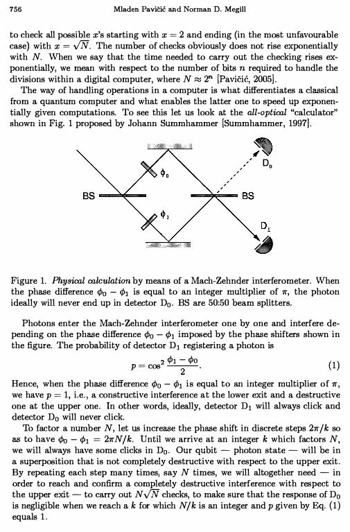


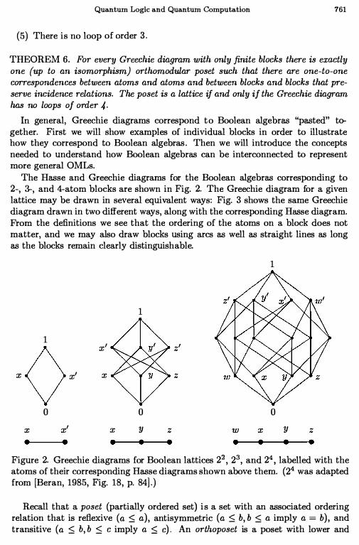


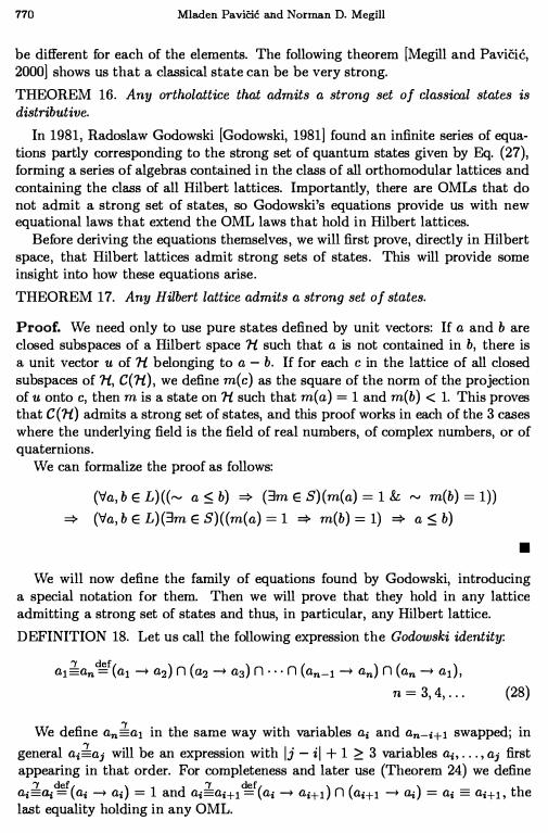

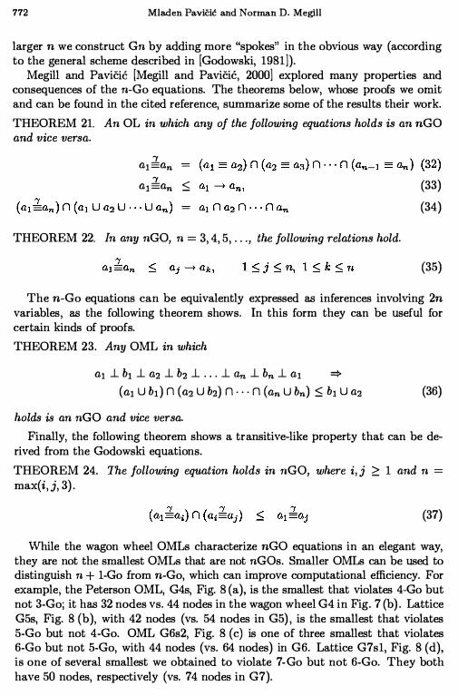


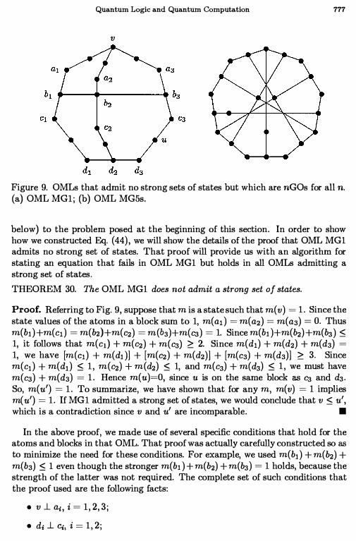


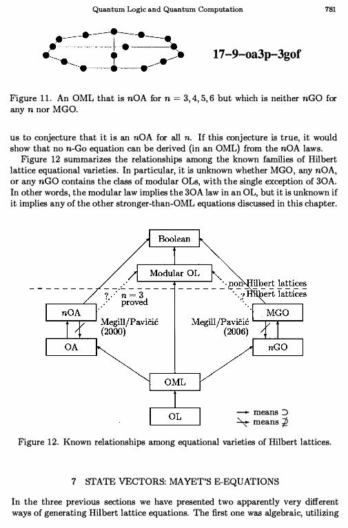

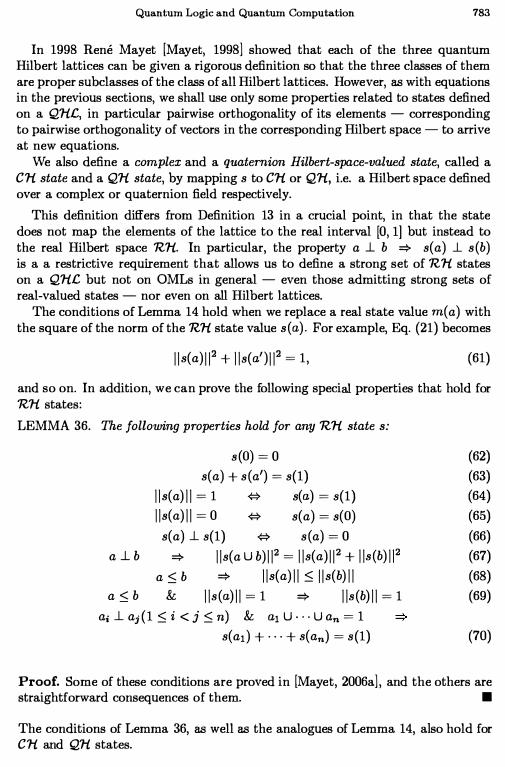


![QUANTUM LOGIC AND QUANTUM COMPUTATION · 2008-04-12 · [4, 6, 10, 11, 42, 43, 50, 58] This quantum logic of qubits (also called quantum computational logic [8, 18]) is a formalism](https://static.documents.pub/doc/80x56/5edc9890ad6a402d666753c9/quantum-logic-and-quantum-computation-2008-04-12-4-6-10-11-42-43-50-58.jpg)


