Page 1
1
HANDLING OF ITEM NON-RESPONSE IN BINARY
VARIABLES: THE RECOVERY STATE OF
CATARACT PATIENTS
BY
ILO, ANTHONY IZUCHUKWU
(PG/M.Sc/06/41106)
BEING A PROJECT SUBMITTED IN PARTIAL FULFILLMENT OF
THE REQUIREMENT FOR THE AWARD OF M.Sc. DEGREE IN
STATISTICS, UNIVERSITY OF NIGERIA, NSUKKA.
NOVEMBER, 2008.
Page 2
2
CERTIFICATION
This work embodied in this project is original and has not been in substance
for any other degrees in this or other Universities.
Supervisor…………………… Head of Department…...…………
Prof. F.C. Okafor Dr. F.I. Ugwuowo
Department of Statistics, Department of Statistics,
University of Nigeria, Nsukka. University of Nigeria, Nsukka.
……………………………
External Examiner
Page 3
3
DEDICATION
This project is dedicated to my beloved parents Mr. Edwin and Mrs Eucharia ILO.
Page 4
4
ACKNOWLEDGEMENT
My profound gratitude goes to the Almighty for His divined providence
throughout this programme. I am thankful to my supervisor Prof. F.C. Okafor, for his
supervisory role in this work. I appreciate in no small measure the contributions of my
lecturers towards creating enabling environment for learning and research.
Worth acknowledging are my colleagues and friends – Jude, Chijindu, Adejoh
Friday, James, Jennifer, Elizabeth, Laurel, Evan, Nduka, Sunday. I also appreciate the
support and encouragement of my brothers and sisters – Godwin, Chukwudi, Mrs
Anthonia Nwosu, Mrs Oluchi Orah, Mrs Uchechukwu Mmaduabuchi and Miss
Chinazaekpere Ilo.
Finally, I am grateful to Prof. J.N Adichie and also to the management and staff
of Eye clinic of Enugu State University of Science and Technology (ESUT) Teaching
Hospital Park-lane Enugu, in particular Dr. Chukwurah, and Dr. Ezegweui – Chief
medical consultant-Eye Clinic of Park- Lane for providing data for this work.
ILO, A.I.
[email protected]
m
08063392492.
Page 5
5
ABSTRACT
Multiple imputation techniques is adopted in this study to compensate for the item
non-response encountered in the sample we collected. This paper described three specific
imputation methods and applied them to the sample of cataract patients data obtained
from Enugu State University of Science and Technology Teaching Hospital Park-Lane
Enugu. The imputation procedures considered are logistic regression imputation model,
random overall imputation and random imputation within classes. The results obtained
from the three imputation methods are similar; showing that analyses of different
imputation methods are consistent. The methods can be used to compensate for item non–
response in similar studies.
Page 6
6
TABLE OF CONTENTS
Title page ……………………….…………………………………….. i
Certification …………….………………………………………….ii
Dedication ……………………………………………………….iii
Acknowledgement ………………………………………….……. iv
Abstract ……………………………………………………….…….. v
Table of contents ………………………………………….……. vi
CHAPTER ONE GENERAL OVERVIEW
1.1 Introduction …………………………………………………1
1.2 Procedures for Creating Multiple Imputations…………. 3
1.3 Explicit and Implicit Models …………………………… 4
1.4 Ignorable and Non-Ignorable Models ……………….……. 4
1.5 Proper Imputation Methods …………………………….4
1.6 Response Mechanism ………………………………….. 5
1.7 Aims and Objectives ………………………………….. 5
1.8 Significance of the study ………………………………….. 5
1.9 Scope and Limitations ………………………………….. 6
CHAPTER TWO LITERATURE REVIEW
2.1 Literature Review …………………………………………..… 7
CAHPTER THREE METHODOLOGY
3.1 Introduction………………………………………………..…..16
Page 7
7
3.2 Missing Data of the Recovery State of Patients………….16
3.3 The Three Basic Imputation Methods Considered………17
3.4 Estimation of the Population Parameters ………………..19
3.5 The Logistic Regression Model…………………………….. 21
3.5.1 Model Specification …………….…………………………. 21
CHAPTER FOUR ANALYSIS
4.1 Introduction ………………………………………………..…. 23
4.2 The Data …………………………………………………..….. 23
4.3 Multiple Imputing for the Missing Values …………..…. 23
4.4 Analysing the Resultant Multiple Imputed Data Sets
for the Three Imputation Procedures………………….…. 27
CHAPTER FIVE DISCUSSION OF RESULT AND
CONCLUSION
5.1 Discussion of Result ………………………………………... 33
5.2 Conclusion …………………………………………………..... 34
References …………………………………………………………….. 35
Appendix I ………………………………………………………….... 37
Appendix II ………………………………………………………..…. 42
Page 8
8
CHAPTER ONE
GENERAL OVERVIEW
1.1 Introduction
Any statistician with experience in the field of survey knows that essentially every
survey suffers from some non response. That is, in practical surveys, some items in the
survey instrument are not answered by all units included in the survey. Commonly, the
items likely to be unanswered are the more sensitive ones, such as those concerning
personal income. An obvious desire of both the data collector and the data analyst is to
get rid of the missing values and thereby restore the ability to use standard complete-data
method to draw inferences. Item non-response may occur in a sample survey because, a
sample unit may refuse or be unable to answer a particular question, or the interviewer
may either fail to ask a particular question or record the answer, or a record is
inconsistent in the sense that it does not satisfy an editing check based on logical or
empirical grounds, etc. The Possible approaches to handling missing values includes: (i)
discarding incomplete cases, (ii) use of weighting adjustment and (iii) imputing the
missing values.
The first option, discarding of incomplete cases, is equivalent to eliminating all
sampled units with at least one value missing. The required estimators are then functions
of values for respondents with complete data only. Although this option is simple and
allows the use of complete file, it presents some risks. Indeed, this option may lead to
strongly biased estimators unless non-response is unrelated to all the variables of interest
(missing completely at random). In addition, by rejecting partial non-respondents,
valuable information from the incomplete responses is not utilized. The sampling weights
cannot be used for inference purpose (unless a weighting adjustment has been applied)
with the result that the inference must be conditional on the sample of complete
respondents. This option should not then be seriously considered other than for a brief
descriptive analysis of the complete respondents.
The second option, weighting adjustment methods may effectively compensate
for partial non-response. These are straight forward, and auxiliary information may be
used wisely to form adjustment classes. The main drawback of weighting adjustment
Page 9
9
methods is that a new adjusted weight must be created for each variable of interest. In
addition, results obtained from different analysis may be inconsistent with each other, the
main reason why weighting adjustment methods are not commonly used to compensate
for partial non-response.
The third and our preferred option for handling non response is imputation.
Imputation simply means assigning one or more real values for each missing responses in
any given sample survey. It is a commonly used method and is a prior, an appealing
general purpose strategy. We chose imputation because it avoids the use of different
weights for estimation. It also reduces the risk of bias in survey estimates arising from
missing data, if it is carefully implemented. Again, by assigning values at the micro level
and thus allowing analyses to be conducted as if the data set were complete, imputation
therefore makes analysis easier to conduct and results easier to present.
Many different procedures have been proposed for imputation, for instance, The
overall mean imputation: this method involves the assigning to the missing response to an
item, the mean of all responses for that particular item obtained from all the other
respondent; The class mean method: this method assigns the average or means value of
the class or group to the missing item; Logical deductive or prior experience method:
here the missing response to an item is deduced with certainty from the pattern of
response to another related item. This method also uses the relationship between
variables to determine a value to be imputed. Other methods are: Random overall
imputation, Random imputation within classes, Sequential hot-deck imputation,
Regression imputation, Distance function matching, Modal imputation and Hierarchical
hot-deck imputation etc. For more details see Kalton and Kasprzyk (1986) and Okafor
(2002 p.348)
In addition to the obvious advantages of allowing complete-data methods of
analysis, imputation by the data collector (e. g the census bureau) also has the important
advantage of allowing the use of information available to the data collector but not
available to an external data analyst such as a university social scientist analyzing a
public use file. This information may involve detailed knowledge of interviewing
procedures and reasons for non-response that are too cumbersome to place on public use
files, or may be facts, such as street addresses of dwelling units, that cannot be placed on
Page 10
10
public-used files because of confidentially constraints. This kind of information, even
though inaccessible to the user of a public-use file, can often improve the imputed values.
Just as there are obvious advantages to imputing one value for each missing value, there
are obvious disadvantages of this procedure arising from the fact, that the one imputed
value cannot itself represent any uncertainly about which value to impute. Hence,
analyses that treat imputed value just like observed values generally underestimate
uncertainty. Equally serious, single imputation cannot represent any additional
uncertainty that arises when the reasons for non response are not known.
In this study, handling of missing cataract data, we adopted the methods of
multiple imputation. Multiple imputation, first proposed in Rubin (1978, 1987), retains
the two major advantages of single imputation and rectifies its major disadvantage. As it
name suggests, multiple imputation replaces each missing value by a vector composed of
M≥2 possible values. The M values are ordered in the sense that the first components of
the vectors for the missing values are used to create one completed data set and so on.
The first advantage of single imputation is retained with multiple imputations, since
standard complete-data methods are used to analyse each completed data set. The second
advantage of imputation, that is, the ability to utilize data collector’s knowledge in
handling the missing values is not only retained but actually enhanced. In addition to
allowing data collectors to use their knowledge to make point estimates for imputed
values, multiple imputation allow data collectors to reflect their uncertainty as to which
value to impute. This uncertainty is of two types; sampling variability assuming the
reason for non response are known and variability due to uncertainty about the reasons
for non response. Under each posited model for non-response, two or more imputations
are created to reflect sampling variability under that model. Imputation under more than
one model for non response reflects uncertainty about the reason for non response.
1.2 Procedures for Creating Multiple Imputation
Multiple imputations ideally should be drawn according to the following general
scheme. For each method being considered, the M imputations of the missing values,
Ymis’ are M repetitions from the values of the respondents, each repetition being an
independent value drawn from the value of the respondent.
Page 11
11
1.3 Explicit and Implicit Models
Explicit models are the ones usually used in mathematical statistics: normal linear
regression, binomial, poisson, multinomial, etc. Implicit models are the ones that can be
thought of as underlying procedures used to "fix up" specific data structures in practice;
often they have a "nonparametric", "locally linear", or "nearest neighbor" flavor to them.
Although explicit models are the theoretical ideal precisely justifying multiple imputation
techniques, often implicit models can be used in place of explicit models. Both types of
models can as well be used together in any study.
1.4 Ignorable and Non-ignorable Models
The models underlying imputation methods, whether implicit or explicit, can be
classified as assuming either ignorable reasons for missing data or non-ignorable reasons.
The term "ignorable" is coined in Rubin (1978) and is fully explicated in the context of
multiple imputation in Rubin (1987). The basic idea is conveyed by a simple example in
which X is observed for all units in the data base, and Y is missing for the non-
respondents but observed for the respondents. An ignorable model asserts that a non-
respondent is only randomly different from a respondent with the same value of X. A
non-ignorable model asserts that even though a respondent and non-respondent appear
identical with respect to X, their Y values systematically differ (e.g., the non-respondent's
Y is typically 20% larger than the respondent's Y with the same value of X). There is no
direct evidence in the data to address the veracity of any such assumption, which is a
good reason to consider several models and explore resultant sensitivity whenever
possible.
1.5 Proper Imputation Methods
Imputation procedures, whether based on explicit or implicit models, or ignorable
or non-ignorable models, that incorporate appropriate variability among the repetitions
within a model are called proper. The essential reason for using proper imputation
methods is that they properly reflect sampling variability when creating repeated
imputations under a model.
Page 12
12
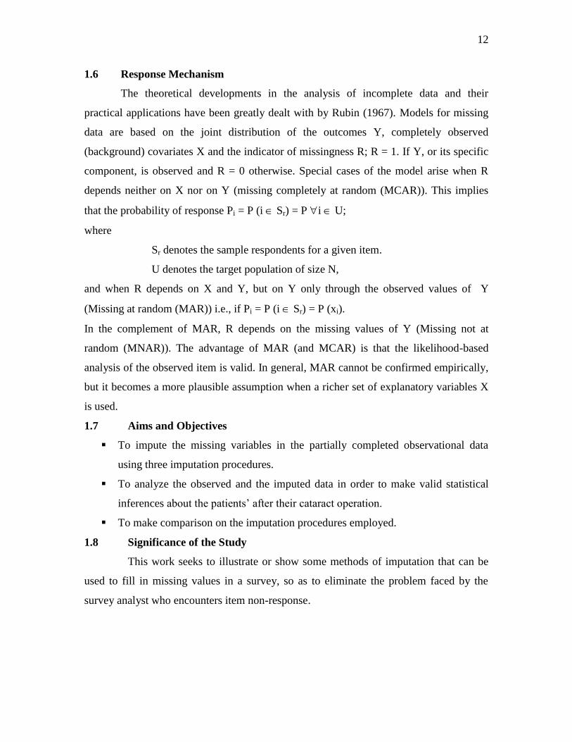
1.6 Response Mechanism
The theoretical developments in the analysis of incomplete data and their
practical applications have been greatly dealt with by Rubin (1967). Models for missing
data are based on the joint distribution of the outcomes Y, completely observed
(background) covariates X and the indicator of missingness R; R = 1. If Y, or its specific
component, is observed and R = 0 otherwise. Special cases of the model arise when R
depends neither on X nor on Y (missing completely at random (MCAR)). This implies
that the probability of response Pi = P (i Sr) = P i U;
where
Sr denotes the sample respondents for a given item.
U denotes the target population of size N,
and when R depends on X and Y, but on Y only through the observed values of Y
(Missing at random (MAR)) i.e., if Pi = P (i Sr) = P (xi).
In the complement of MAR, R depends on the missing values of Y (Missing not at
random (MNAR)). The advantage of MAR (and MCAR) is that the likelihood-based
analysis of the observed item is valid. In general, MAR cannot be confirmed empirically,
but it becomes a more plausible assumption when a richer set of explanatory variables X
is used.
1.7 Aims and Objectives
To impute the missing variables in the partially completed observational data
using three imputation procedures.
To analyze the observed and the imputed data in order to make valid statistical
inferences about the patients’ after their cataract operation.
To make comparison on the imputation procedures employed.
1.8 Significance of the Study
This work seeks to illustrate or show some methods of imputation that can be
used to fill in missing values in a survey, so as to eliminate the problem faced by the
survey analyst who encounters item non-response.
Page 13
13
1.9 Scope and Limitations
This study focuses on handling of missing cataract data using multiple
imputation techniques, employing binary logistic regression imputation model, random
overall imputation method and random imputation within classes. We systematically
sampled 160 patients’ case files from the records obtained from Enugu State University
of Science and Technology (ESUT), Teaching Hospital Park-Lane Enugu, from January
1998 to December 2007. However, some of the findings, predictions and suggestions
from the analysis of data may be restricted to the affected area. In addition, the risk
factors were not exhausted as we considered only those that are the likelihood factors to
recovering. The main limitation of our methodology is the failure to account for the so
called non-ignorable non-response, which arise when the distribution of respondents and
non-respondents on an incomplete variable differs, even after conditioning on values of
observed variables. Another limitation is the lack of “correct” imputed values. This paper
is based on real data with real non response. It is not base on simulated data in which the
missing data mechanism is known.
Page 14
14
CHAPTER TWO
LITERATURE REVIEW
Although imputation techniques have not been used widely, a number of
applications pertaining to demographic and health research has appeared in the statistical
literature. In this chapter we review some of the scholarly work done in the areas of
imputation.
Greenless et al (1982) proposed a means of treating or handling missing response
in a case where the response mechanism is not ignorable, the case in which the
probability of non-respondent for the variable of interest depends upon values of that
variable. They show different ways in which missing values can be treated. The
approaches include:
(i) To ignore the non-response problem and use the complete observations as a
“sample”.
(ii) Finding the estimate with incomplete sample survey data.etc
Unfortunately, all these approaches are systematically in error, since the probability of
response varies with Y, a case that is very rarely considered explicitly but sometimes
seems reasonable. In this article, they propose to test on a particular data set the
usefulness of a “stochastic censoring model” similar to those referenced earlier, for
imputing when the probability of response depends on the variable being imputed, here
they imputed income when the probability of response depends upon income. In which
the data from the March 1973 current population survey (CPS) are matched with
administrative data from the social security Administration (SSA) and the internal
revenue service (IRS).
Based on the assumption that the variable of interest Yi is regressed on the vector of
auxiliary variable Xi, they applied the logistic regression model. The maximum likelihood
of the parameters of the model can be found by numerically maximizing the log of this
function with respect to the given parameters Yi, Zi and Xi. Given the estimated
parameters of the model, they impute individual non respondents’ Y values by assigning
the mean of the distribution of Y conditional on non-response values of Z and X for that
individual and the maximum likelihood parameter estimates. The result obtained from
Page 15
15
this approach is consistent. They concluded that the stochastic censoring approach to
imputing missing values has potential for improving on commonly used imputation
procedure that rely on the assumption that the probability of non response does not
depend on the variable being imputed. Application of this method requires a model of the
determination of the variable of interest and a model of the non response mechanism.
Lepkowski et al (1987) analyzed imputed data from a sample survey: the National
Medical Care Utilization and Expenditure Survey (NMCUES) which was designated to
collect data about the United States civilian non institutionalized population in 1980’s.
Using a stratified multi-stage sample of households, information were obtained on health,
access to and use of medical service, associated charges and sources of payment, and
health insurance coverage through interviews. Individuals in a sampled household were
interviewed four to five times over one year period in 1980 and 1981. However, for the
key survey items such as health care expenditures, income and other sensitive topics, the
amount of item missing data for the responding persons was substantial, and this missing
data varied considerably across items. Since imputation for all items with missing data
would have been expensive, imputation were made on important demographic, economic
and expenditure items. The methods used to impute data for missing values were diverse
and tailored to measures requiring imputation. Three types of imputation predominated in
this paper they are: Deductive, Sequential hot-deck and weighted sequential hot-deck
imputation methods. Deductive or logical imputations were used to eliminate missing
data that could be determined readily from other data items that provided overlapping
information. (This might even be referred as edits). Details on how deductive imputation
assigns value to the missing values were stated in the article. The sequential hot-deck was
use primarily for small number of imputations on demographic items. In the sequential
hot-deck procedure, the data are grouped into within imputation classes and then sorted
within those classes by measures that are correlated with the item for which imputations
are to be made. The detailed procedures are also in the paper. Finally, the weighted
sequential hot deck imputation was used most extensively to provide impute values for a
variety of measures, many of which had substantial amount of missing data.
Since extensive imputations were made for missing values for a large number of
the key items in the NMCUES, they are expected to influence estimates made from the
Page 16
16
survey in several ways. They presented a result which demonstrates the effect that
imputations have on the estimates. They recommend researchers on survey data with
imputation for substantially important survey items to select a strategy for handling
imputation in estimation. They presented four different strategies for handling imputed
survey data which the result of there paper allows. For a large complex survey like theirs,
they recommend that strategy, 1 which “use all the data, real as well as imputed, in all
analysis” be followed, with significant attention given to an investigation of the effect of
imputation on analysis.
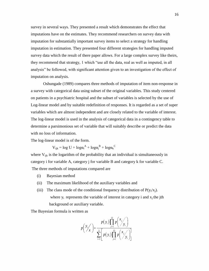
Oshungade (1989) compares three methods of imputation of item non-response in
a survey with categorical data using subset of the original variables. This study centered
on patients in a psychiatric hospital and the subset of variables is selected by the use of
Log-linear model and by suitable redefinition of responses. It is regarded as a set of super
variables which are almost independent and are closely related to the variable of interest.
The log-linear model is used in the analysis of categorical data in a contingency table to
determine a parsimonious set of variable that will suitably describe or predict the data
with no loss of information.
The log-linear model is of the form.
Vijk = log U + logαiA + logαj
B + logαk
C
where Vijk is the logarithm of the probability that an individual is simultaneously in
category i for variable A, category j for variable B and category k for variable C.
The three methods of imputations compared are
(i) Bayesian method
(ii) The maximum likelihood of the auxiliary variables and
(iii) The class mode of the conditional frequency distribution of P(yi/xj).
where yi represents the variable of interest in category i and xj the jth
background or auxiliary variable.
The Bayesian formula is written as
13
1
133
1 1
ji
iji
ji
ii j
xp y p
yyp
x xp y p
y
Page 17
17
and the predicted category for a non-response will be that category with the largest values
of the three posterior probabilities.
The method of the maximum likelihood of the background variables is similar
to the Bayesian method except that it does not make use of any prior probability or an
equiprobable prior, instead the likelihoods. The probability of occurrence of any
independent variable xj in each of the categories i of the variable of interest yi is the
likelihood L of that particular independent variable given the category of the variable of
interest, ie,
L (xj/yi) = P (xj/yi)
The assumption of independence of xj enables them to take
L(xj/yi) = P(x1/yi) P(x2/yi) . . . P(xj/yi)
Since they are using xj in each category i of the variable y. They define W(yi) as being
dependent on the value of L(xj/yi)
W(yi) = K L(xj/yi)
where, K is the factor of relationship
13
1
j
ij
xw y k p
y
, i = 1,2,3.
Then, the i category with the maximum value of W(yi) is the prediction.
The method of direct use of the modal category from the distribution of P(yi/xj)
starts by dividing the population of respondents into classes based on the item responses
x that are common to both the respondents and non respondents. Then a modal category
of the responses conditioned on x are assigned to the missing item. It was observed that
the Bayesian method is preferable although there is little or no difference from that of the
maximum likelihood method. The use of modal category is not as efficient as either of
these two methods.
Heitjan D. F and Little R. J. A. (1991) carried out an analysis on the fatal accident
reporting system (FARS). The methods of multiple imputations were employed on the
data collected, which contains a considerable number of non responses. The fatal accident
reporting system is a database for the US National Highway Traffic Safety
Administration (NHTSA) collected at the site of all fatal traffic accidents. Variables
include location and time of accident, number and position of vehicle, age, sex and
Page 18
18
driving record of driver, seat-belt use and blood alcohol content of the driver. The last
two variables are of great interest but have substantial proportions of missing data. They
explores the use of multiple imputations based on predictive mean matching as a means
of achieving the aim of NHTSA which is to fill the missing data in order to obtain
reliable estimates. Predictive mean matching is an example of a hot-deck method, where
the values of the non-respondents are imputed using values of the respondents matched
with respect to some metric. However, since blood alcohol content (BAC) is of primary
analytical interest and has easily the highest level of non response, this paper therefore
focuses on BAC. The metric for matching the complete and incomplete cases is based on
regression of the following variables on non-missing predictors.
0 BAC if 0,
0 BAC if 1, 1Test
0 BAC if Missing,
0 BAC if BAC, 2Test
They embark on the estimation of the regression of Test 1 and Test 2 on all variables
except BAC. The method of multiple imputation, an extension of imputation proposed by
Rubin (1978, 1987) where M > 1 set of values are drawn from the predictive distribution
to the missing values. The method involves only standard regression software and a fairly
easily programmed matching algorithm, which makes good use of available information
on incomplete records to fill all the missing values and this largely met the goal of a good
imputation procedure. In particular, they provide the means for assessing the impact of
impute by presenting a set of five imputes for each missing value. An implementation on
a subsample of FARS data illustrates the fact that the observed covariate have some
predictive power for imputing missing BAC values, particularly when police reported
alcohol involvement, is available. Also a simulation study Monte Carlo results confirmed
that the method provided substantial improvement over single imputation methods.
Longford et al (2000) conducted an observational prospective survey study on the
subject born in the 3rd
to 9th
week of March, 1946. The outcomes studied are derived
from the entries in diaries of food and drink intake over seven designated days. Since
interest of the paper is to handle missing data in diaries of Alcohol Consumption. The
background variables and other variables related to alcohol consumption and associated
Page 19
19
problems are used as collateral information. The objective of the study was to assess the
extent of problems with alcohol in the cohort of subject born in 1946 in Great Britain.
The amount of alcohol consumed is commonly regarded as a suitable scale for this. In
this perspective, the average amount consumed for various subpopulations and their
comparisons are the quantities of interest. On the assumption that the outcomes studied
are missing at random given the background variables. Multiple imputation technique is
used here as a tool for compensating for missing responses to outcome variables, which
are in turn used for generating the imputed values of the missing diary items. Values are
also imputed for body mass which is not available for some subjects; also the above
assumption is adopted for the body mass within the four categories defined by cross-
classification of sex and smoking status. The imputations are generated from a model
which relates the multivariate outcomes, the covariates and the incidence of missingness.
Since the outcome variables is a binary, the model is logistic regression model, which is
used to compensate for the missing variables. The main result obtained from this analysis
is an estimate of the proportion of the population who has consumed more than a given
amount of alcohol. In the estimation, the diary entries are regarded as valid and their
conversion to quantities of net alcohol as precise. In conclusion, they noticed a vast
difference between the prevalence of excessive alcohol consumption of men and women,
even when the criterion for excessive consumption is sex specific and taking account of
body mass.
Myunghee et al (2000) carried out a survey on the analysis of missing covariate
variables. The study is an on-going prospective population based incidence designated to
identify risk factors for strokes among white, blacks and hispanics in a survey called the
Northern Manhattan Stroke Study (NOMASS). Matched case-control data are used to
make for the missing covariates. In this case-control study of NOMASS, controls were
matched for each case based on age, race and sex. The goal of the study was to examine
the protective effect of physical activity on stroke after adjusting for already known risk
factor and whether physical activity remains protective after adjusting for the level of
High Density Lipoprotein (HDL). Analysis of the study faced difficulty because the HDL
level was not available for all subjects. The analysts tried four different methods of
Page 20
20
handling missing HDL data and the resulting estimates are biased and some methods
cannot be applied in this type of survey.
In the study, they develop an imputation estimation approach motivated from an
approximated conditional likelihood. This proposed method is valid under the missing at
random (MAR) mechanism. The observation indicator for X is denoted by r;
otherwise 0,
observed is x if 1, r
The probability of the missingness may depend on observed data, (Y,W,Z) but not on X,
ie,
Pr(r = 1/X, W, Y, Z) = Pr ( r = 1/W, Y, Z)
In this case study, X is the HDL level and the components of Z are age, race and sex
which is the matching variables for matched set and Y is the case indicator for subjects in
the matched set. They assumed that the linear logistic disease prevalence model, given as
Logit [ Pr(Y = 1/W, X, Z) ] = + 1Tw + B2X + q(Z)
is valid in the population from which case and control are drawn. Coefficient = (1T
,
2)T is the log odd-ratio parameter of primary interest. The NOMASS data are analyzed
by using the method proposed, where the missing HDL values are replaced with a
function of the predicted values from a regression model for case and controls.
Winglee et al (2001) show-case some methods of handling item non-response in a
sample survey: the US component of IEA reading literacy study. The study was
coordinated by the International Association for the Evaluation of Educational
Achievement (IEA). The methods of imputation used to assign value to the missing
variables were the Hot-deck imputation and modal imputation methods. The most straight
forward way to analyse the complete data file is proceded as if the data were actually
reported. The study provides an empirical assessment of the impact of imputation on such
a secondary data analysis. In particular, regression analysis and Hierarchical linear
modeling (HTM) analysis were conducted on the data sets that used different methods for
handling missing data and the result were compared. The results from regression models
estimated from the data set completed by imputation, were compared with the
corresponding models estimated using three other methods of handling missing data.
These other methods were; the complete case (C.C) analysis (Case wise deletion
Page 21
21
method); the Available case (A.C) analysis (Pair wise deletion method) and the
Estimation maximization E.M. algorithm. The study shows that data analysis using hot-
deck imputed data yielded similar results to those produced by A.C and E.M methods of
handling the missing data. The result however is different from those produced by C.C.
method. They recommend the use of hot-deck imputation for such likely studies, since
analysis with hot-deck imputed data is simple to implement.
Revicki et al (2001) discussed ways of compensating for the missing health
related quality of life (HRQOL) outcomes on physical health status, scores missing
owning to mortality. Having missing data complicates the statistical analysis of HRQOL
data and depending on the extent and nature of missing data, significant bias can be
introduced in the treatment comparisons. They evaluated the bias associated with 4
different imputation methods used in estimating physical health status (PHS), scores
missing as a result of mortality. The imputation methods were; last value carried forward
(LVCF); arbitrary substitution (ARBSUB); empirical Bayes (BAYES) and within subject
modeling (WSMOD). Simulation studies were conducted in which they systematically
varied mortality rates from 0% to 30% and change in PHS scores from –20 to 20 on a
100-point scale for a 2-group clinical trial with follow-up over 18 months. Pseudo-root
mean square residuals and difference between true and estimated slopes were used to
evaluate how well the imputation methods reproduced the true characteristic of the
simulated population data. The difference imputation methods produced comparable
results when there were few missing data. The BAYES approach most closely estimated
true population difference and change in PHS regardless of missing data rates.
Coen et al (2003) conducted an analysis on a cancer screening survey data with 2
continuous, 48 linkers scale items and 74 binary response items. This research team
conducted a randomized effectiveness trial of a quality improvement intervention, to
increase colorectal cancer (CRC) screening rate within providers’ organizations that
contract with large California health maintenance organizations that targets the primary
care providers, nurses and administrative staff to improve the rate at which enrolled
patients utilized CRC screening tests. This survey centered on the comparison of two
multiple imputation procedures by applying them to the survey, that is, the CRC
intervention study. For each multiple imputation strategy five complete data sets were
Page 22
22
created. In the study 1340 questionnaires were mailed to potential respondents of which
891 returned the questionnaires. Of the 891 returned questionnaires, 9 from respondents
who indicated that they did not provide primary care were dropped from further analysis.
All returned questionnaires had at least 49 of 136 completed items. The missing data
mechanisms were known and no assumption was made about them. The methods they
used for multiple imputations consisted of:
(a) Hot-deck and regression methods and
(b) Multivariate normal multiple imputation.
For the hot-deck method, they drew one donor case at random from the complete
case, for the five donor cases. In the regression method, three separate regression models
were used for imputation, that is, linear, logistic and generalized linear regression. Here
the missing covariates were imputed using hot-deck procedure. They used one set of
covariates for all regression models. The advantage of this is that imputations are easier
to produce compared to building different regression models for different variables. The
model was estimated using all the observed response, and next, the missing responses
were imputed by predicting it through the observed covariate.
The second method which is imputations by assuming a multivariate normal
distribution on all variables jointly is a common method for multiple imputations.
Imputed data set are obtained in two steps. First the mean vector and the covariance
matrix are obtained using Estimation Maximization Algorithm. Second, with the obtained
estimates, data augmentation is carried out in order to obtain multiple imputed values.
They also illustrated how the point and interval estimates from the multiple imputed data
sets are obtained, which can also be found in Rubin (1986). The results of both methods
of imputation were found to be similar; either of the two methods is endorsed for surveys
similar to the data set.
Page 23
23
CHAPTER THREE
METHODOLOGY
3.1 Introduction
In this chapter, we make a general overview and description of the statistical
methods governing this research. We also describe our problem of missing data in greater
details, outlines the three basic multiple imputation procedures used in this situation and
also give the statistical formulas used in the imputation.
Since the interest of this work is on handling of item non-response in the recovery state
of patients’ after cataract operation, using the likely factors associated with recovery.
This recovery could be measured in terms of the probability of patients transiting from
one level of visual acuity (VA) to the other. Again since imputation is our preferred
option for treating item non response, we present an application of multiple imputation
using the data obtained from Eye clinic of Enugu State University of Science and
Technology (ESUT) Teaching Hospital, Park-Lane Enugu, from 1998 to 2007, to analyse
the recovery state of patients after the cataract operation. Multiple imputation is a
technique used for treating missing responses in a survey. In this approach rather than
assigning a single value to an incomplete observation, we replace each missing value
with four values. The value imputed is a binary indicator of whether the patient recovers
from the operation or not. Inferences are then made by using the full data set, and also
repeated for each distinct data file associated with each set of imputed values. Statistics
are computed by averaging over the set of complete-sample estimates.
3.2 Missing Data of the Recovery State of Patients
The data for this study was obtained from the Eye clinic of ESUT, Teaching
Hospital, Park-Lane Enugu, on the records of patients at the hospital from January 1998
to December 2007, who have been discharged by the end of the year 2007. One of the
objectives of the data was to record the number of admission and outcomes after a
cataract operation in the hospital. Items recorded for each patient admitted in the hospital
includes, year of admission, unit number, sex, age, marital status, date of operation,
Page 24
24
haemoglobin content of the patient (Hb), plasma glucose, blood pressure, any other
ocular disease (AOOD), occupation, follow up dates and outcomes. Out of 800 patients’
case files, 20% were systematically sampled from the population within the period.
Throughout this study we considered only four of the variables which are considered here
as likelihood factors to recovery. The outcomes which is the state of recovery of the
patients after the operation, witnessed a number of non response and were to be predicted
using these four variables and the value of the respondents. It was observed that out of
the 160 selected records, that the outcomes of 16 patients were not recorded resulting in a
10% missing responses. We assume that the item responses for the respondent and the
non respondents are broadly similar, that is, the missing observations are missing at
random. Then the non respondents were assigned an appropriate value using the
procedure discussed below.
3.3 The Three Basic Imputation Methods Considered
In this study we will consider three multiple imputation models, one explicit and
two implicit imputation models. They are Logistic regression imputation model, Random
overall imputation and Random imputation within classes.
The explicit multiple imputation models consist of three basic steps. The first step, we
specify a model to predict the value of a missing variable, y. In this study the predicted
model is a binary logit regression model as given by Freedman and Douglas (1995)
yi =
otherwise 0,
μ βx if 1, j (3.1)
where x is a vector of observed variables, is a vector of parameters to be estimated, and
is a random variable that follows the extreme value distribution. The choice of binary
logistic regression stems principally on the dichotomous nature of the response
(dependent) variable. This model will also enable us predict a discrete outcome
(recovered or not recovered) from a set dichotomous, discrete and continuous
independent variables.
We estimate the parameter vector using the proportion of the sample with
complete data. Given an estimate of and value for x, y can be predicted with (3.1) by
Page 25
25
drawing a value of from the extreme value distribution, equivalently, y can be predicted
using the relationship
yi =
otherwise 0,
μ )xβ(logit if 1, j (3.2)
where
Logit βx exp 1
βx exp xβ
j
j
j
(3.3)
and follows the Bernoulli (0, 1) distribution.
In the second step, we carry out several “rounds” of imputation; the number of
rounds is denoted as k. Each round of imputation produces a value of yik for each
incomplete observation. Each round uses a distinct value of kβ common across all
imputed cases and drawn independently from the multivariate distribution of the
estimated vector . Moreover, each imputed value of yik depends on an independently
drawn value of μ . The number of imputation rounds we carried out were 4, ie
k=1,2,3,4; which is considered adequate. The stochastic imputation procedure associated
with (3.2) occasionally assigns yi = 0 when pr(yi = 1) is high, and occasionally assigns yi
= 1 when the corresponding probability is low.
The multiple imputation procedure thus preserves one source of uncertainty about
the process underlying the observed y, conditional on the parameter vector .
Randomization of the parameter vector in the second step of the imputation process
reflects an additional source of uncertainty: although the observed values of y are
postulated to be generated by a process represented by (3.1), here we have only an
estimate based on sample data instead of the true value of the population parameter .
The second stage of the imputation process embodies our uncertainty about the value of
.
In the third and final step of the imputation process, we analyze the k distinct data
set of the observed and the imputed data, and combine the k alternatives estimates of the
statistics of interest. For the k completed data sets we first obtain the k point estimates of
the proportion of patients that recovered after the cataract operation. Since the state of
Page 26
26
recovery of the patients is our variable of interest and also a dichotomous variable, it
should therefore be noted that proportion is the mean of a dichotomous variable.
The implicit multiple imputation method considered is: Random overall
imputation method; which assigns a value from the respondent selected at random to the
non-respondents. Each donor respondent is selected at random from the total respondents
in the sample. This method is the simplest form of hot-deck imputation, that is, an
imputation procedure in which the value assigned for a missing response is taken from a
respondent to the current survey.
Another implicit imputation method, is the Random imputation within classes: in
this hot-deck imputation method a respondent is chosen at random within an imputation
class, and the selected respondent’s value is assigned to the non respondent. That is the
total sample is first divided into classes, then the random imputation is carried out within
the classes. In this study we used gender to form the imputation classes.
3.4 Estimation of the Population Parameters
Considering a simple random sample of size n selected from N population units
without replacement. The estimator of the population proportion, P is given as
p* = cc*
i
n
1 iy
n
n y
n
1
(3.4)
where,
p* is the sample proportion of patients that recovered after the operation with
imputed data.
n is the sample size
nc is the number of patients that recovered
*
iy is the observed and imputed values of the recovered patients
cy = p*
We also estimate the sampling variance of the proportion, kS , for the k complete data
sets.
q*p 1 -n
f - 1
1 -n
q*p
N
n - N Sk (3.5)
where
q = 1 – p*
Page 27
27
N is the population units
f = n/N is the sampling fraction.
The under-listed estimates are as given by Rubin (1986) for multiple imputation
The final estimate of the proportion based on the combination of all the k completed data
sets of the proportion is
*
k
k
1 ip
k
1 p
(3.6)
where, p is the overall proportion of patients that recovered after the cataract operation
in the k rounds of imputation
The within imputation variance, W of the k completed data sets equals
k
k
1iS
k
1 W
(3.7)
The between imputation variance, B is the variance between the point estimates,
2k*
k
1 ip - p
1 -k
1 B
(3.8)
The combined estimate for the variance, based on both the within, W and the between,
B imputation variances forms what we called the total variance denoted as T,
T = W + (1 + k-1
) B (3.9)
where the factor (1 + k-1
) multiplying the unbiased estimate of between imputation
variance is an adjustment for using a finite number of imputations,
The relative increase in variance due to imputation, is defined as
= (1 + k-1
) B / W (3.10)
The tests and confidence interval are based on student t-approximation.
tTp ~ p -* (3.11)
with degree of freedom equal to
= (k-1) (1 + -1
)2 (3.12)
The fraction of missing information about p, due to non response is denoted as ,
= 1
3) (2
(3.13)
Page 28
28
For single imputation, the estimate of the proportion of patients that recovers after the
cataract operation is given as
mrs mPrPn
P 1
(3.14)
Where
Pr is the sample proportion of patient’s that recovered based on r respondents.
Pm is the sample proportion based on m missing values.
While the sample estimator of the variance for single imputation, ignoring the finite
population correction as given by Rao and Shao (1992) is
n
S
n
m
r
nTs
*
(3.15)
Where
S* is the sample variance obtained from the complete data set with the
imputed values. It is conditional unbiased for S2, hence Ts is approximately
unbiased.
3.5 The Logistic Regression Model
3.5.1 Model Specification
Logistic regression is part of a category of statistical models called generalized
linear models. This broad class of models includes ordinary regression and ANOVA as
well as ANCOVA and log linear regression. Logistic regression allows one to predict a
discrete outcome, such as group membership, from a set of variables that may be
continuous, discrete, dichotomous, or a mix of any of these. Generally, the dependent or
response variable is dichotomous, such as presence/absence or success/failure. As
mentioned above, the independent or predictor variables in logistic regression can take
any form, that is, logistic regression makes no assumption about the distribution of the
independent variables.
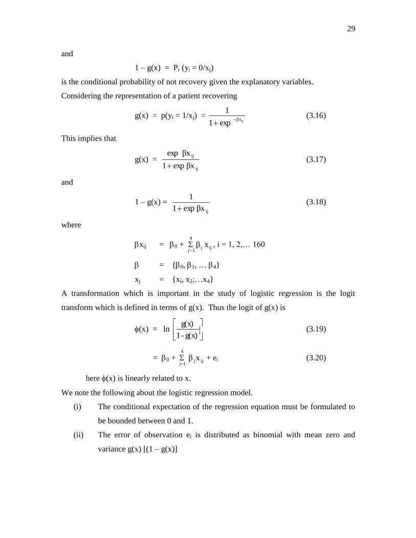
Assuming that there are j explanatory variables x = {x1 x2,…xj}. The outcome
variable yi is a binary variable indicating whether a patient recovers (y=1) or not (y=0). If
the conditional probability that a patient recovered given the explanatory variables is
denoted by g(x)
g(x) = pr (yi = 1/xj)
Page 29
29
and
1 – g(x) = Pr (yi = 0/xj)
is the conditional probability of not recovery given the explanatory variables.
Considering the representation of a patient recovering
g(x) = p(yi = 1/xj) = exp 1
1ijβx -
(3.16)
This implies that
g(x) = ij
ij
βx exp 1
βx exp
(3.17)
and
1 – g(x) = ijβx exp 1
1
(3.18)
where
xij = 0 + ijj
4
1 xβ
j
, i = 1, 2,… 160
= {0, 1, … 4}
xj = {xi, x2;…x4}
A transformation which is important in the study of logistic regression is the logit
transform which is defined in terms of g(x). Thus the logit of g(x) is
(x) = ln
g(x) - 1
g(x) (3.19)
= 0 + ijj
4
1jxβ
+ ei (3.20)
here (x) is linearly related to x.
We note the following about the logistic regression model.
(i) The conditional expectation of the regression equation must be formulated to
be bounded between 0 and 1.
(ii) The error of observation ei is distributed as binomial with mean zero and
variance g(x) [(1 – g(x)]
Page 30
30
CHAPTER FOUR
ANALYSIS
4.1 Introduction
In this section, we multiple imputed the recovery state of cataract patients’ data
missing in the observed data, using the proportion of the sample patients that responded.
We fit a binary logistic regression model to the proportion of patients that responds from
which we employ our first imputation technique. For the other imputation procedures we
used the values of the respondents
4.2 The Data
The data for this study were obtained from 160 patient’s case files systematically
sampled from the records of eye clinic of ESUT Teaching Hospital Park-Lane Enugu,
from January 1998 to December 2007. Measurement of the best visual acuity of patients
taken after operation is based on the critical examination of the eye by the physician’s.
The parameters used to determine the state of recovery of a patient after operation upon
serious examinations were as follows.
A - Light perception
B - Hand movement
C - Counting of fingers
D - Direction of Objects
E - Use of figures etc.
In order to fit a logistic regression model, the response variables (outcomes of
patients’ vision) were taken through the check-up visits after the operation. Thus the
outcome is binary with codes 0 for “not recovered” and 1 for “recovered”. Recovery here
means that a patient satisfy all tests after operation. The explanatory variables include
factors that potentially influence the likelihood of recovery and were available in each
patients file. The variables obtained from each patient files are shown in the appendix.
4.3 Multiple Imputing for the Missing Values.
In order for us to impute the missing responses using logit regression model, we
first obtain the estimate of parameters of the model using the observed values of the
Page 31
31
patients that responded. Recall, that the transform of our logistic regression model is of
the form.
(x) = 0 + 1xi1 + 2xi2 + 3xi3 + 4xi4 + ei
where ’s is the model parameters
x1 = gender, x2 = Haemoglobin content (Hb)
x3 = Glucose x4 = Any other ocular Disease (A.O.O.D)
ei = error in observation.
The table below displays the result obtained in fitting a binary logistic regression model,
using a statistical computer package called SPSS.
Table 1: The Estimates of the Parameter of the Logistic Regression Model Using the
Observed Values of Patients that Responded.
Variables
Gender -.206
Hb -.018
Glucose .005
A.O.O.D .235
Constant -1.070
Using (3.2) and following the second step of imputation for logit regression model, we
impute all the missing responses in the observed variables.
The tables below shows the result of the multiple imputed data sets, four, for each
of the 16 missing responses.
The result of multiple imputation for missing data in the observed variables applying the
logistic regression model predicted in section 3.3 using (3.2) are shown in Table 2
Here we illustrate how logit regression model yielded the results below.
For the first missing value
Logit ( jxβ ) = 13.5 0.018-
13.5 -0.018
e1
e
= 0.93 > 0
So we impute 1
Page 32
32
Table 2
The Result of Multiple Imputation for Missing Data in the Observed Variables
Applying the Logistic Regression Imputation Model
S/N Missing
Observation
Imputed Values
A B C D
1 8 1 0 1 0
2 19 0 0 0 0
3 37 0 0 0 0
4 41 1 0 0 1
5 47 1 1 0 0
6 56 1 0 1 0
7 68 0 0 0 0
8 71 1 0 0 0
9 85 1 0 0 0
10 96 0 0 0 0
11 110 1 1 0 0
12 116 0 1 1 1
13 136 1 0 0 1
14 141 0 1 0 0
15 148 1 0 0 0
16 159 0 1 0 1
Page 33
33
TABLE 3
The Result of Multiple Imputation for the Missing Data in the Observed Variables
Applying Random Overall Imputation Method.
S/N Missing
Observation
Imputed Values
A B C D
1 8 0 1 0 1
2 19 1 1 1 1
3 37 0 1 1 1
4 41 0 1 0 0
5 47 0 0 1 1
6 56 1 1 0 1
7 68 1 1 1 1
8 71 1 1 0 0
9 85 0 0 0 0
10 96 0 0 0 1
11 110 1 0 0 0
12 116 1 0 1 0
13 136 0 0 0 0
14 141 0 0 1 0
15 148 0 0 0 1
16 159 0 0 0 1
Page 34
34
TABLE 4
The Result of Multiple Imputation for the Missing Data in the Observed Variables
Applying Random Imputation within Classes Method.
S/N Missing
Observation
Imputed Values
A B C D
1 8 1 0 1 1
2 19 1 1 0 1
3 37 0 0 0 1
4 41 1 1 0 1
5 47 1 0 1 1
6 56 1 1 0 0
7 68 1 0 0 0
8 71 1 1 0 0
9 85 0 0 0 0
10 96 1 1 0 0
11 110 0 1 0 0
12 116 0 1 0 1
13 136 0 1 0 1
14 141 0 0 1 0
15 148 1 1 1 1
16 159 0 1 0 1
4.4 Analysing the Resultant Multiple-Imputed Data Sets for the Three
Imputation Procedures.
Each set of imputations, that is, each column of Tables 2, 3 and 4 are used for the
incomplete data in Table 11, to create a complete data set. Since there are four sets of
Page 35
35
imputations, four complete data sets are created for each imputation technique; these
tables are also displayed in the appendix.
Using (3.4), and (3.5) in each of the four completed data sets of the three
imputation methods, the estimates of the proportion and its variance, for the patients that
recovered after the cataract operation were
Table 5
Estimate of the Multiply Imputed Data Sets, of Tables 12-15 in the Appendix Using
Logit Regression Model
Proportions (*
ikp ) Variance of proportion ( kS )
1 0.3563 0.0012
2 0.3313 0.0011
3 0.3188 0.0011
4 0.3250 0.0011
Table 6
Estimate of the Multiply Imputed Data Sets, of Tables 16-19 in the Appendix Using
Random Overall Imputation Method
Proportions (*
ikp ) Variance of proportion ( kS )
1 0.3375 0.0011
2 0.3438 0.0011
3 0.3375 0.0011
4 0.3563 0.0012
Page 36
36
Table 7
Estimate of the Multiply Imputed Data Sets, of Tables 20-23 in the Appendix Using
the Method of Random Imputation within Classes
Proportions (*
ikp ) Variance of proportion ( kS )
1 0.3563 0.0012
2 0.3625 0.0012
3 0.3250 0.0011
4 0.3563 0.0012
The combined estimates of the proportions, its variances and other estimates for
the multiply imputed data sets of Tables 5-7 are obtained using equations 3.6, 3.7, 3.8,
3.9, 3.10, 3.12 and 3.13, which are shown below in the Tables 8-10.
Illustration of how the combined estimate of the proportions and its variances
were obtained using equations 3.6, 3.7, 3.8 and 3.9 in Table 5. are
p = *4
14
1ik
ip
= 4
1 (0.3563 + 0.3313 + 0.3188 + 0.3250)
= 4
1.3314
= 0.3329
Page 37
37
0011.0
0045.04
1
0011.00011.00011.00012.04
1
4
1 4
1
^
i
kSW
00135.0
00025.00011.0
0002.0410011.0
41
0002.0
0000656094.03
1
3329.03263.0
3329.03250.03329.03313.03329.03563.0
14
1
14
1
1
1
2
222
4
1
2*
BWT
PPBi
i
Page 38
38
Table 8
The Combined Estimates and Variances for Complete Data Sets of Table 5. (Logit
Regression Model).
Estimates Results
Single multiple
1 Proportion ( p ) 0.2756 0.3329
2 Within variance ( W ) - 0.0011
3 Between variance ( B ) - 0.0002
4 Total variance (T) 0.00001 0.0014
5 Relative increase in variance due to
imputation ()
- 0.2273
6 The degree of freedom for interval
estimates of p constructed using
t-distribution ()
- 87.46
7 Fraction of missing information about p
()
- 0.0201
Table 9
The Combined Estimates and Variances for Complete Data Sets of Table 6.
(Random Overall Imputation)
Estimates Results
Single multiple
1 Proportion ( p ) 0.2738 0.3438
2 Within variance ( W ) - 0.0011
3 Between variance ( B ) - 0.0001
4 Total variance (T) 0.00001 0.0012
5 Relative increase in variance due to
imputation ()
- 0.1136
6 The degree of freedom for interval
estimates of p constructed using
t-distribution ()
- 288.29
7 Fraction of missing information about p
()
- 0.0065
Page 39
39
Table 10
The Combined Estimates and Variances for Complete Data Sets of Table 7.
(Random Imputation within Classes)
Estimates Results
Single multiple
1 Proportion ( p ) 0.2756 0.3500
2 Within variance ( W ) - 0.0012
3 Between variance ( B ) - 0.0003
4 Total variance (T) 0.00001 0.0016
5 Relative increase in variance due to
imputation ()
- 0.3125
6 The degree of freedom for interval
estimates of p constructed using
t-distribution ()
- 53.24
7 Fraction of missing information
about p ()
- 0.0313
Page 40
40
CHAPTER FIVE
DICUSSION OF RESULT AND CONCLUSION
5.1 Discussion of Result
Without knowing what the missing values exactly would be if they had been
observed, it is impossible to say if analysis from single or multiple imputed data set
equals the complete data set. Four sets of imputations were properly created under each
of the three imputation methods used to impute the missing cataract data, the results are
displayed in Tables 2, 3 and 4.
We observed from the estimates of proportion and variances for single and multiple
imputation, that imputation really makes analysis from different methods consistent. The
estimates of the proportion of patient’s that recovered after the operation under each
imputation methods were approximately, 28%, 27%, and 28% for single imputation and
33%, 34% and 35% for multiple imputation. The estimate of the proportion of patients’
that recovers, for single imputation procedures were obtained using (3.14).
For the estimates of the variance of proportion, the singly imputed data variances
obtained using (3.15) is typically too small to compare to the variances of multiple
imputed data sets. This is because single imputation is known to overstate precision.
Irrespective of the obvious advantages of multiple imputation to single imputation, this
small variance is as a result that single imputation does not reflect the between imputation
variance. Apart from the estimate of proportion and its variance single imputation cannot
produce any other valid inference for other estimates which multiple imputation does.
For the three multiple imputation methods, point estimates of the proportion, within
and between imputation variance, total variance, degree of freedom for interval estimates,
and fraction of missing information were computed.
For the estimate of variance, in multiple imputed data sets, though negligible
differences exist in the within and between imputation variances, it can generally be seen
that the total variance for the random overall imputation is smaller followed by logit
regression model imputation method and lastly the random imputation within classes.
The estimates for the degree of freedom, are all large, indicating that the student’s t-
approximation of (3.11) is essentially a normal one. Note that these degree of freedom
Page 41
41
does not depend on the sample size but on the number of imputation K and the ratio of
the between imputation variance, B to within imputation variance, W .
For the estimated fractions of missing information, ƒ in each imputation method, we
notice that if Ymis carried no information about P, then the imputed-estimates *P would
be identical and T would be reduced to W .
5.2 Conclusion
In this study we performed a thorough and proper practical imputation analysis on
the content of missing cataract data. The imputation methods we considered are logistic
regression imputation model, random overall imputation and random imputation within
classes. Since the proportion of missing values is more than 5%, single imputation is not
quite reasonable, without special corrective measures, because single imputation
technique do not account for uncertainty about which value to impute and also do not
preserve the sampling variability. Following this shortcoming we recommend multiple
imputation for any survey researcher with missing survey data above 5% of the sample.
The great virtues of multiple imputation are its simplicity and generality. The user may
analyse the data by virtually any technique that would be appropriate if the data were
complete. The validity of the method, however, hinges on how the imputations
k
mismis YY ...,,)1( were generated. Clearly it is not possible to obtain valid inferences in general
if imputations are created arbitrarily. The imputations should on average, give reasonable
predictions for the missing data, and the variability among them must reflect an
appropriate degree of uncertainty.
We also recommend that for missing survey data similar to that presented in this paper,
either of the three imputation methods should be adopted.
Page 42
42
REFERENCES
Coen. A. B. Melissa M. F; Karen Q.I; Gareth S. D; Patricia A. G; Katherine L.K (2003).
Comparison of Two Multiple Imputation Procedures in a Cancer Screening
Survey. Journal of Data Science Vol. p. 1-20.
Cox D. R. and Snell E. J (1989). Analysis of Binary Data, 2nd
ed. Chapman & Hall.
Damodar N. Gujarati (2003). Basic Econometrics Fourth Edition. Tata McGraw. Hill.
Freedman Vicki A; and Douglas A.W. (1995). A Case Study on the use of Multiple
Imputation. Demography; “Population Ass. Of America” Vol. 32, No 3, P. 459-
470.
Greenless J.S; William S. R, Kimberly D. Z. (1982). Imputation of Missing Values When
the Probability of Response Depends on the Variable Being Imputed. Journal of
the American Statistical Ass. Vol. 77, No. 378. p. 251-261.
Heitjan D.F and Roderick J.A. Little (1991). Multiple Imputation for the Fatal Accident
Reporting Systems Applied Statistics, Vol. 40, No 1. p. 13-29.
Kalton G. and Kasprzyk (1986). The treatment of missing survey data. Survey
methodology Journal of Statistics Canada vol. 12, No. 1. p. 1-16.
Lepkowski J.M; Richard Landis Sharon A. S. (1987). Strategies for the Analysis of
Imputed Data from a Sample Survey: Medical Care, Vol. 25. No.8. p. 705-716.
Longford N.T; Margaret Ely; Rebecca H; Michael E.J.W. (2000). Handling Missing Data
in Diaries of Alcohol. Series A. Vol 163, No 3 p. 381-402.
McCullagh P. and Nelder J.A. (1989). Generalized Linear Models 2nd
ed. Chapman &
Hall.
Myunghee C.P. and Ralph L. Sacco (2000). Matched Case Control Data Analysis with
Missing Covariates. Applied Statistics, Vol. 49, No. 1. p 145-156.
Okafor F.C. (2002). Sampling Survey Theory with Applications. Afro-Orbis pub. Ltd.
Onyeka C.A. (1996). Introduction to Applied Statistical Methods. 7th
Ed. Nobern
Avocation Pub. Company
Oshungade Olayiwola Isacc, (1989). Some Methods of Handling Item Non-Response in
Categorical Data. The Statistician, Vol. 38, No. 4. p. 281-296.
Page 43
43
Press J.S; and Sandra Wilson (1978). Choosing Between Logistic Regression and
Discriminant Analysis. Journal of American Statistical Association Vol. 73, No.
364, p 699-705.
Revicki D. A; Karen G; Dennis B; Kitty Chan; Joel D. K; Michael J. W. (2001).
Imputing Physical Health Status Scores Missing Owing to Mortality: Result of a
Simulation Comparing Multiple Techniques. Medical Care Vol. 39, No. 1. p. 61-
71.
Roderick J.A. Little (1982). Models for Non response in Sample Surveys. Journal of
American Stat. Ass. Vol. 77, No. 378. p. 237-249.
Rubin D.B. (1978) Multiple Imputation in Sample Surveys---a phenomenological
Bayesian approach to non-response, Proceedings of the section on Research
Methods, Journal of American Statistical Association, pp, 20-28
Rubin D.B. (1986). Basic Ideas of Multiple Imputation for Nonresponse. Survey
Methdology. Journal of Statistics Canada Vol 12, No 1, p. 37-48.
Rubin D.B. (1987). Multiple Imputation for Nonreesponse in Surveys. New York: Wiley
Winglee Marianne; Graham K; Keith R; Daniel K. (2001). Handling Item Nonresponse in
the U.S. Component of the IEA Reading Literacy Study. Journal of Educational
and Behavioural Statistics Vol. 26, No 3, P. 343-359.
Page 44
44
APPENDIX I
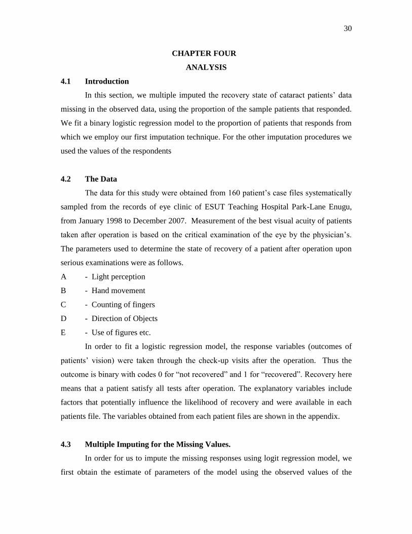
Table 11: The Observed Variables
Observation Outcome (y) Gender Hb Glucose A.O.O.D
1 0 1 18.0 180 1
2 0 1 17.5 101 0
3 0 1 13.5 170 1
4 1 1 16.5 113 1
5 0 0 16.5 120 1
6 0 1 17.5 60 1
7 0 1 16.5 74 0
8* . 0 11.5 105 1
9 0 0 11.5 160 0
10 0 1 18.0 60 0
11 0 1 16.5 116 1
12 0 1 17.5 90 1
13 0 0 14.5 89 1
14 0 1 12.5 95 1
15 0 0 16.5 90 0
16 1 0 12.0 140 0
17 0 1 13.0 70 1
18 0 0 14.5 134 1
19* . 0 13.0 110 1
20 1 0 11.5 113 1
21 0 1 13.0 68 0
22 0 0 13.0 109 1
23 1 1 16.5 100 0
24 0 0 13.0 70 0
25 0 1 13.0 75 1
26 0 0 16.5 89 1
27 0 1 16.5 175 0
28 0 1 16.5 110 1
29 0 0 16.5 170 0
30 0 0 11.5 68 0
31 0 1 12.0 75 0
32 0 1 12.5 120 0
33 1 1 12.5 110 0
34 0 0 13.5 59 0
Page 45
45
35 1 0 16.5 101 1
36 1 1 16.5 180 1
37* . 1 13.0 74 1
38 1 1 13.5 140 0
39 0 1 12.0 60 0
40 0 1 18.0 125 1
41* . 1 14.0 130 0
42 0 1 12.5 90 1
43 1 0 11.5 95 0
44 0 0 14.0 160 1
45 0 1 13.0 90 1
46 1 1 12.5 140 1
47* . 1 17.5 60 0
48 0 0 14.0 90 1
49 0 0 11.5 150 1
50 1 0 14.0 150 1
51 0 0 16.5 138 0
52 0 1 15.5 110 0
53 0 1 18.0 96 1
54 0 1 16.5 100 0
55 0 1 17.5 119 1
56* . 0 12.0 124 1
57 0 1 14.5 160 0
58 1 0 12.0 100 0
59 0 1 12.5 90 1
60 1 0 12.0 90 0
61 0 1 12.5 140 1
62 1 1 16.5 96 0
63 1 1 12.5 114 1
64 0 0 11.5 180 0
65 1 1 13.5 160 1
66 0 1 16.0 74 0
67 1 1 16.0 120 0
68* . 0 15.0 180 1
69 0 1 17.5 130 1
70 0 1 13.0 58 0
71* . 1 13.5 100 1
72 0 1 13.0 77 0
Page 46
46
73 0 1 14.5 89 1
74 1 1 18.0 180 1
75 0 1 12.0 70 1
76 0 0 14.0 74 1
77 0 1 12.5 79 1
78 0 0 15.5 98 0
79 1 1 16.0 120 1
80 0 0 12.5 100 1
81 0 1 13.0 120 0
82 0 1 16.5 140 0
83 1 1 16.5 72 1
84 1 0 12.0 110 0
85* . 1 15.5 130 1
86 0 1 16.5 70 0
87 0 0 16.5 155 0
88 1 0 16.5 82 1
89 1 0 16.5 100 1
90 1 0 13.5 124 0
91 0 0 13.5 190 0
92 0 1 15.5 70 1
93 1 0 16.5 120 1
94 0 0 12.0 190 0
95 0 1 11.5 70 0
96* . 0 12.0 80 1
97 0 0 13.0 120 1
98 1 0 11.5 180 1
99 0 1 17.5 65 0
100 0 0 13.0 70 1
101 0 1 18.0 95 1
102 1 1 16.0 170 1
103 1 1 16.5 65 1
104 0 0 13.5 134 0
105 0 1 13.0 100 0
106 0 0 15.5 74 1
107 0 1 12.5 160 1
108 0 0 12.0 204 1
109 1 1 12.5 110 1
110* . 1 12.5 84 1
Page 47
47
111 1 1 15.0 125 0
112 1 1 16.5 74 1
113 0 0 14.0 134 0
114 1 0 15.0 130 0
115 0 0 12.0 100 1
116* . 0 11.5 60 0
117 1 1 13.5 110 1
118 0 1 14.5 122 1
119 0 0 16.5 80 1
120 0 1 13.5 180 0
121 1 0 16.0 120 1
122 1 1 12.5 100 0
123 1 0 11.5 160 1
124 0 1 13.5 124 1
125 1 1 13.5 90 0
126 1 0 16.5 134 0
127 0 1 15.5 190 1
128 1 0 12.0 65 0
129 0 1 17.5 84 1
130 1 0 16.5 135 1
131 0 0 14.0 120 1
132 0 1 16.5 84 1
133 0 0 11.5 100 1
134 0 1 15.5 120 0
135 0 0 15.5 165 1
136* . 1 16.5 65 0
137 0 1 14.0 200 1
138 1 1 17.5 190 1
139 0 1 15.5 100 0
140 1 1 14.5 60 1
141* . 0 16.5 119 0
142 1 0 12.0 65 1
143 0 0 11.5 70 1
144 0 1 13.5 160 0
145 1 0 11.5 130 1
146 1 1 15.0 100 1
147 0 0 16.5 70 1
148* . 0 12.5 90 1
Page 48
48
149 0 1 12.5 170 1
150 0 1 17.5 160 0
151 0 0 13.0 167 1
152 0 1 13.5 71 0
153 0 1 17.5 90 0
154 1 1 16.0 163 0
155 0 1 17.0 60 0
156 1 0 11.5 110 1
157 1 1 12.5 160 0
158 0 0 12.5 66 0
159* . 0 11.5 98 1
160 0 0 15.5 80 0