Radioastronomy with a TV-satellite dish

Lab Course M at I. Physics Institute of the Universitat zu Koln

V. 1.4, March 10, 2012

1 Introduction

The aim of the experiment Radioastronomy with a TV-satellite dish is to determine thetemperature of the sun. With the small radio telescope on the roof of the institute wemeasure radiation emitted by the sun. To interprete the measured data and to finallydetermine the physical temperature, we need to calibrate the measurement system.

This experiment relies on the knowledge taught in the experimentMicrowave Radiome-

ter. Therefore, it is advisable to work through these two experiments in the appropriatesequence.

The basic knowledge of antenna physics and the physics of electromagnetic radiationneed to be prepared in advance.

2 Preparation

In particular you should have a working knowledge of the following concepts:

2.1 Basics

• Black body radiation

• Rayleigh–Jeans approximation, Wien’s law

• Absorption and emission of radiation

• Basics of celestial mechanics, satellite orbits

• Optics: single slit diffraction

We recommend to use radioastronomical literature for the preparation [1, 2], since theyemphasize the connection between the fundamental laws of physics and their applicationin astronomy.

2.2 Specific concepts and techniques of radioastronomy

These topics should be prepared with the help of the literature cited below.

• Reciprocity theorem

• The sun as a radio source

• The atmosphere’s influence on electromagnetic radiation (radio window)

• Airmass (path length through the atmosphere)

1

• Antenna pattern

• Techniques to determine the antenna pattern

• Correction factors (efficiencies) in the antenna pattern

• Antenna temperature

• Relationship between the antenna pattern and the contributions to the antennatemperature

• Calibration of the antennea temperature

• Receiver noise

• Y-factor calibration

• Heterodyne principle.

The questions of section 3 should be prepared for the day of the experiment and needto be answered in the written report.

The report has to be submitted as hardcopy, and, if it is prepared using a typesettingprogram, the final version (after all corrections) also has to be submitted electronically(LATEX, OpenOffice or Word-Format – not PDF).

2

2.3 Theory

Properties of the radiation In radio astronomy one normally deals with incoherentradiation. This means that the radiation consists of a mixture of statistically independentwaves with different frequencies and phase.

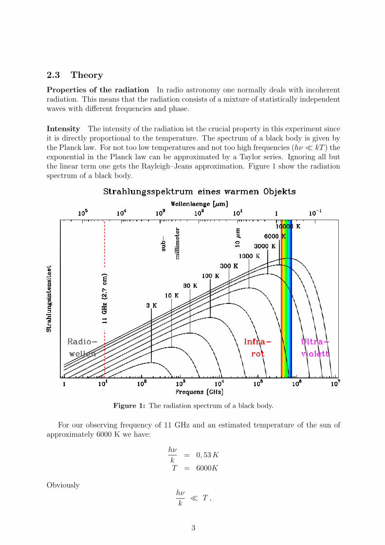
Intensity The intensity of the radiation ist the crucial property in this experiment sinceit is directly proportional to the temperature. The spectrum of a black body is given bythe Planck law. For not too low temperatures and not too high frequencies (hν ≪ kT ) theexponential in the Planck law can be approximated by a Taylor series. Ignoring all butthe linear term one gets the Rayleigh–Jeans approximation. Figure 1 show the radiationspectrum of a black body.

Figure 1: The radiation spectrum of a black body.

For our observing frequency of 11 GHz and an estimated temperature of the sun ofapproximately 6000 K we have:

hν

k= 0, 53K

T = 6000K

Obviouslyhν

k≪ T ,

3

showing that the Rayleigh-Jeans approximation is good enough. Within this approxima-tion the intensity and temperature are directly proportional to each other. This is thereason that in radioastronomy the two quantities are often used synonymously.

Absorption und emission of radiation Although the intensity B is independent ofthe the distance to the source, it can be modified along the path of propagation x. Bothabsorption and emission may affect the intensity. The reduction of the intensity throughabsorption in a medium (e.g a cloud) is given by:

B = B0 e−τc . (1)

B0 is the intensity before entering the medium, τc is the optical depth. For a constantabsorption coefficient α of the medium τc may be written as αx. The emission by themedium is given by:

Bc = Bi (1− e−τc). (2)

Bi is the source function of the cloud’s emission. Thus, a cloud that is both, emitting andabsorbing, the total intensity is

B = B0 e−τc + Bi (1− e−τc) (3)

Expressed in units of temperature this is:

T = T0 e−τc + Tc (1− e−τc), (4)

where Tc is the temperature of the cloud. In a real case this equation describes for examplethe temperature of a source observed through the atmosphere.

The reciprocity theorem The reciprocity theorem state that the radiation character-istics of an antenna is idependent of whether it is used as a receiving or a transmittingantenna. This is equivalent to the fact that in optics a light path can be reversed.

Antenna calibration The voltage measured by the ADC board in the measurementcomputer is directly proportional to the power received by the telescope.

VADC = c Tsys (5)

Tsys = TA + Trec (6)

Tsys is the system temperature, as measured through the receiver. it is composed of thereceiver’s intrinsic noise temperatur (Trec) and the external signal TA. c is a proportianal-ity constant, which has to be determined by the calibration. Trec can be obtained fromthe Y-factor calibration.

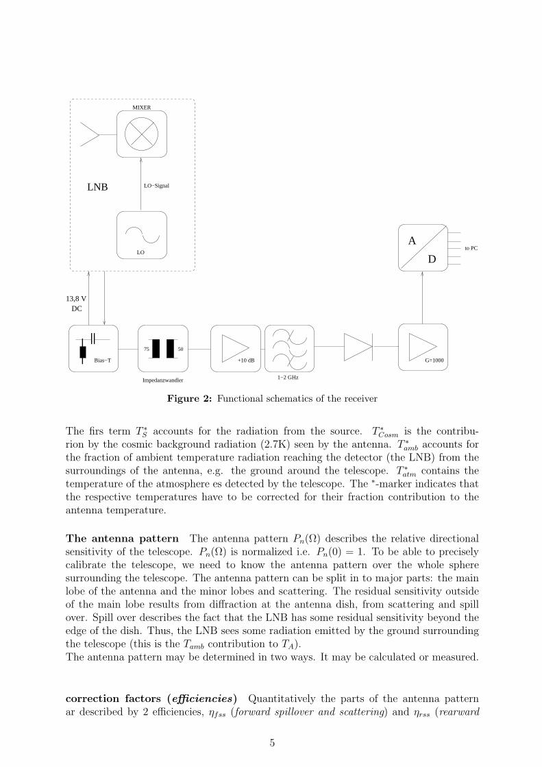
The antenna temperature TA is the so called antenna temperature. To deduce theproperties of the observed source from this quantity, one needs to know exactly the signalscontributing to TA (Abb. 5).

TA = T ∗

S + T ∗

Cosm + T ∗

amb + T ∗

atm. (7)

4

LNB

Bias−T

Impedanzwandler

75 50

+10 dB G=1000

A

D

1−2 GHz

LO

MIXER

to PC

LO−Signal

13,8 VDC

Figure 2: Functional schematics of the receiver

The firs term T ∗

S accounts for the radiation from the source. T ∗

Cosm is the contribu-rion by the cosmic background radiation (2.7K) seen by the antenna. T ∗

amb accounts forthe fraction of ambient temperature radiation reaching the detector (the LNB) from thesurroundings of the antenna, e.g. the ground around the telescope. T ∗

atm contains thetemperature of the atmosphere es detected by the telescope. The ∗-marker indicates thatthe respective temperatures have to be corrected for their fraction contribution to theantenna temperature.

The antenna pattern The antenna pattern Pn(Ω) describes the relative directionalsensitivity of the telescope. Pn(Ω) is normalized i.e. Pn(0) = 1. To be able to preciselycalibrate the telescope, we need to know the antenna pattern over the whole spheresurrounding the telescope. The antenna pattern can be split in to major parts: the mainlobe of the antenna and the minor lobes and scattering. The residual sensitivity outsideof the main lobe results from diffraction at the antenna dish, from scattering and spillover. Spill over describes the fact that the LNB has some residual sensitivity beyond theedge of the dish. Thus, the LNB sees some radiation emitted by the ground surroundingthe telescope (this is the Tamb contribution to TA).The antenna pattern may be determined in two ways. It may be calculated or measured.

correction factors (efficiencies) Quantitatively the parts of the antenna patternar described by 2 efficiencies, ηfss (forward spillover and scattering) and ηrss (rearward

5

Figure 3: Schematic antenna pattern in polar (logarithmic) representation. The red partindicates the sensitivity in the forward half sphere, consisiting of main lobe and minorlobes. The green part represents the sensitivity in the rear half sphere, which is caused byspill over effects.

spillover and scattering):

ηfss =

∫∫ΩD

Pn(Ω) dΩ∫∫

2πPn(Ω) dΩ

= 66% (8)

ηrss =

∫∫2π

Pn(Ω) dΩ∫∫4π

Pn(Ω) dΩ= 87% (9)

ΩD is the solid angle covered by the main lobe. The 2π integrals extend over the forwardhalf sphere. Thus, ηfss is the fraction of power detected within the main beam comparedto the total power detected from the forward half sphere. ηrss is is the fraction of powerdetected from the forward half sphere compared to the total power received.

For simplicity, we often approximate the main beam by a two-dimensional Gaussiandistribution.

Coupling efficiency If the source is smaller than the main beam, we need to take intoaccount that only a fraction of the radiation detected by the antenna originates from thesource. Thus, we need to estimate, what fraction ηc of the main lobe is filled by the

6

source: (Abb. 4):

ηc =

∫∫ΩD

Tn,Source(Ω)Pn(Ω) dΩ∫∫

ΩD

Pn(Ω) dΩ. (10)

Tn,Source is the normalized temperature distribution of the source. We assume a constantcircular distribution, i.e. Tn,Source is equal to 0 within the area of the solar disk and 0outside of the disk.

Figure 4: Coupling efficiency ηc versus source size expressed in units of the beam width.Only the dark colored fraction of the antenna pattern receives radiation from the source.

With the assumption of a Gaussian main beam and a disk-like source with constanttemperature, it is possible to calculate ηc analytically.

Effects of the atmosphere When measuring with a ground based telescope, the trans-parency of the earth’s atmosphere is a crucial factor. The atmospheric transmission de-pends strongly on the wavelength. There are mainly two atmospheric windows suitablefor astronomic observations from the ground: the optical regime and the so-called radiowindow. The radio window covers the frequency range from approximately 20 MHz to300 GHz. At the low frequency end, the electron density of the ionosphere limits thetransmission. Ultra violet radiation from the sun partly ionizes the atmosphere. Thiscreates free electrons, which block the propagation of radiation below a certain frequency.

The upper limit of the radio window at around 300 GHz originates from absorption byatmospheric molecules, such as water or oxygen. This is the reason to put observatoriesfor mm-wave astronomy on on high mountain tops with thin and dry air.

7

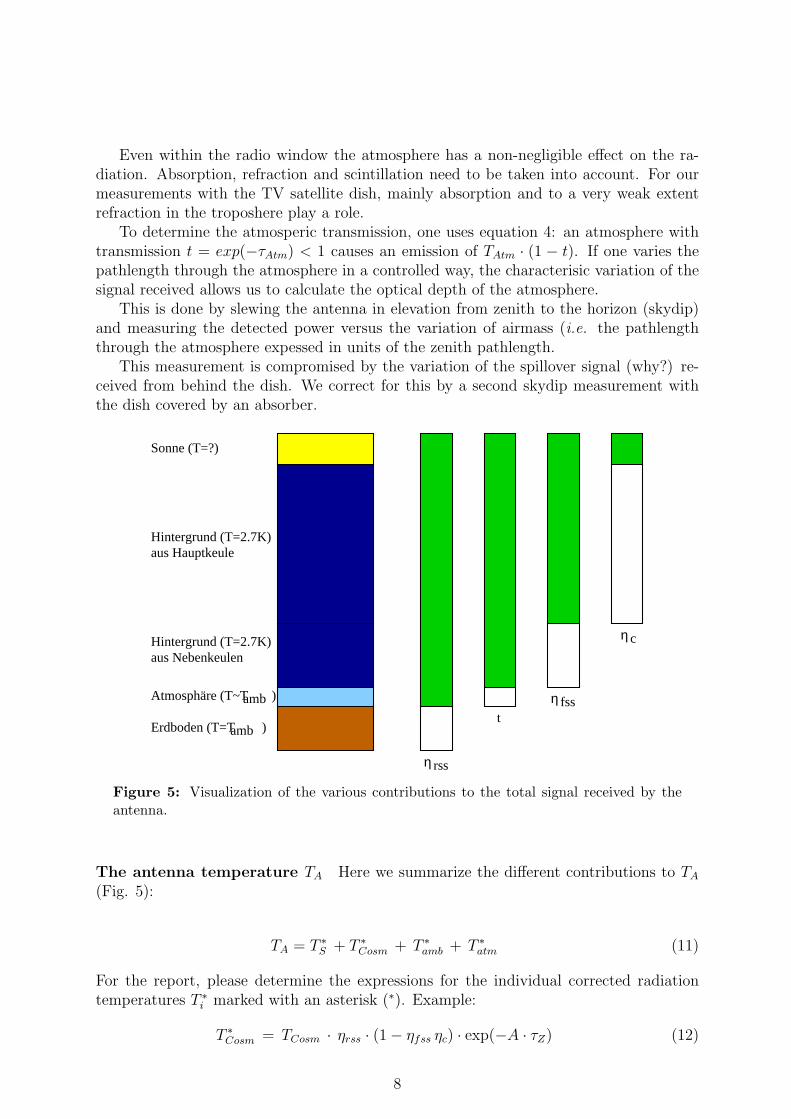
Even within the radio window the atmosphere has a non-negligible effect on the ra-diation. Absorption, refraction and scintillation need to be taken into account. For ourmeasurements with the TV satellite dish, mainly absorption and to a very weak extentrefraction in the troposhere play a role.

To determine the atmosperic transmission, one uses equation 4: an atmosphere withtransmission t = exp(−τAtm) < 1 causes an emission of TAtm · (1 − t). If one varies thepathlength through the atmosphere in a controlled way, the characterisic variation of thesignal received allows us to calculate the optical depth of the atmosphere.

This is done by slewing the antenna in elevation from zenith to the horizon (skydip)and measuring the detected power versus the variation of airmass (i.e. the pathlengththrough the atmosphere expessed in units of the zenith pathlength.

This measurement is compromised by the variation of the spillover signal (why?) re-ceived from behind the dish. We correct for this by a second skydip measurement withthe dish covered by an absorber.

aus NebenkeulenHintergrund (T=2.7K)

Hintergrund (T=2.7K)aus Hauptkeule

η rss

η c

η fss

Sonne (T=?)

t

Atmosphäre (T~T )

Erdboden (T=T )

amb

amb

Figure 5: Visualization of the various contributions to the total signal received by theantenna.

The antenna temperature TA Here we summarize the different contributions to TA

(Fig. 5):

TA = T ∗

S + T ∗

Cosm + T ∗

amb + T ∗

atm (11)

For the report, please determine the expressions for the individual corrected radiationtemperatures T ∗

i marked with an asterisk (∗). Example:

T ∗

Cosm = TCosm · ηrss · (1− ηfss ηc) · exp(−A · τZ) (12)

8

This means that the physical temperature TCosm for the forward direction gets correctedby a factor ηrss (87%) and for the atmospheric absorption by exp(−A · τZ). The part ofthe radiation detected from the sun is subtracted.

Establish the corrections for the other contributions to TA.

3 Questions

Answer the following questions. Make reasonable assumptions where required.

1. Give the orbital periods of some terrestrial satellites: ISS, ASTRA, moon. Calculatethe respective orbital radii.

2. Estimate the width of the antenna main beam (Hint: reciprocity theorem, diffrac-tion). The telescope diamter is 1 m.

3. Estimate the width of the antenna main beam of your eye (yes!). What does itmean?

4. Derive the formula for the coupling coefficient ηc assuming a Gaussian main beamand a concentric circular constant temperature source.

5. Estimate the coupling coefficient ηc,sun between the antenna main beam and thesun.

6. Estimate the coupling coefficient ηc,ASTRA between the antenna main beam and theASTRA satellite.

7. What is the relation between atmospheric transmission and antenna elevation (fitfunction for the skydip measurement)?

4 Measurements

Carry out the following measurements:

1. Map a satellite. Required commands:pos astra.in: select a satellite as the source.measure map 9 0.6: Map the satellite (i.e. the antenna main beam) with a 9×9–pixel map using 0.6 degrees pixel spacing.

2. Calibration of the antenna temperature using liquid nitrogen and ambient temper-ature. Cover the detector’s field of view first with a liquid nitrogen dewar and thenwith a room temperature absorber. The LNB shold be looking down, which can beachieved with the command pos cal.in. This makes the telescope slew to zenith.Data acquisition starts with the command measure stare 500 (“Stare at whateveris visible for 500 seconds”). Before the calibration measurement the ambient tem-perature absorber should spend some time outside to reach a stable temperature.Measure the outside temperature with a thermometer.

9

3. Skydip:pos skydip.in: moves the antenna to a feature free part of the sky.measure table skydip 2.table: read offset positions from the file skydip 2.table

and take a measurement at each position.

4. Repeat skydip with covered antenna. Cover the dish with the large absorber.

5. Map the sun: pos SUN.in, measure map 9 0.6.

We do the sun measurement several times. After this series, we repeat the calibrationand the skydips. Try to make all measurement without unneccessary delay. Drifts in themeasurement conditions by adversly affect your data.

5 Measurement data and report

First we determine the coupling efficiency between the sun and the antenna pattern.The coupling integral will be calculated analytically from the width of a Gaussian fit tothe satellite map. The remaining efficiency factors are given above. The atmospherictransmission is obtained from the skydip measurement. First we have to subtract therearward spill-over measurement from the actual skydip data. The function defined insection 3 is fitted to the resulting data to deduce the zenith optical depth.

Gaussian fits to the maps of the sun yield the difference of the antenna temperaturemeasured on the sun and on the surrounding sky. Applying equation 11 in an suitableway to this difference, the temperature of the sun can be deduced.

To calculate the atmospheric transmission we use the zenith optical depth and theelevation of the sun during the measurement. If needed, the elevation can be reconstructedusing the creation date of the data file of a measurement.

6 Using the system

The measurement setup is controled by a Linux PC, which communicates with the antennadrive system and digitizes the measurement data using an ADC extension board.

6.1 Processes

Several processes need to run during an observation to control and synchronize the sub-systems:

• astra server continuously calculates the position coordinates of the source. To beable to accurately track a moving astronomical object like the sun, it needs to knowthe exact time, which is ensured by an NTP network time sychronization.

• tracker server controls the positioning of the antenna. It reads the coordinatescalculated by astra server and drives the dish to the desired position.

• greg is a data visualization program used in radio astronomy to graphically displaythe measured data.

10

6.2 Commands

• pos: Selects the object to be tracked. Syntax: pos XYZ.in. XYZ may be any ofSUN MOON astra hotbird eutelsat cal skydip. pos cal puts the antenna inan orientation suitable for the hot-cold calibration where the LNB is accessible withthe liquid nitrogen dewar. pos skydip selects an azimuth position where neitherhigh buildings nor satellites are encountered.

• measure: Starts a measuerement. Syntax: measure <command> X [Y],where <command> is one of the following:

h, help: Display this messagec, cross: Take a cross scan with X by X points spaced by Yx, xline: Take a horizontal line scan with X points spaced by Yy, yline: Take a vertical line scan with X points spaced by Ym, map: Take a map with X by X points spaced by Ys, stare: Take X measurements at current position, with a frequency of 1 Hzt, table: Take one scan at each offset in file X (or stdin)

The data are stored in the directry daten, which is expected to be an existingsubdirectory of the directory where measure measure was started.

• Kset fp: Command to control low-level parameters of the system. This commandis only used to correct pointing offsets, which may be encountered when changingsources. Syntax:

– Kset fp: lists all available parameters and their current values.

– Kset fp <par>: displays the value of parameter <par>. Relevant parametersare a poa (pointing offset in azimuth) and a poe (pointing offset in elevation).

– Kset fp <par> <val>: sets the value of parameter <par> to the value <val>.For instance Kset fp a poe -2300 sets the elevation correction to -2300 arc-seconds.

• gaussfit: Calculates the best fit Gaussian to a data set measured with measure

m N deg. Syntax: gaussfit < datafile. The output contains the start values ofthe fit parameters and the best fit values. This out put may be redirected into afile using gaussfit < datafile > fitfile.

7 Literatur

References

[1] J. D. Kraus, Radio Astronomy, Cygnus-Quasar Books, 1986.

[2] O. Hachenberg and B. Vowinkel, Technische Grundlagen der Radioastronomie,Mannheim; Wien; Zurich: Bibliographisches Institut, 1982., Wien, 1982.

11

[3] “KOSMA: Kolner Observatorium fur SubMillimeter Astronomie”,(http://www.ph1.uni-koeln.de/gg/).

[4] “NANTEN2 (Chile)”, (http://www.ph1.uni-koeln.de/workgroups/astro instrumentation/nanten2/).

[5] “SOFIA: Stratosperic Observatory For Infrared Astronomy”,(http://www.sofia.usra.edu).

12