Hans Huang: Regional 4D-Var. July 30th, 2012 1 Regional 4D-Var Hans Huang NCAR Acknowledgements:...

Hans Huang: Regional 4D-Var. July 30th, 2012 1

Regional 4D-Var

Hans Huang

NCAR

Acknowledgements: NCAR/MMM/DAS

USWRP, NSF-OPP, NCAR

AFWA, KMA, CWB, CAA, EUMETSAT, AirDat

Dale Barker (UKMO), Nils Gustafsson and Per Dahlgren (SMHI)


• 4D-Var formulation and “why regional?”

• The WRFDA approach

• Issues specific to regional 4D-Var

• Summary

Outline


4D-Var

J = Jb + Jo

Jb =1

2x0 - xb T B 1 x0 - xb

Jo =1

2yk H M k x0

TR 1 yk H M k x0

k


Why 4D-Var?

• Use observations over a time interval, which suits most asynoptic data

and uses tendency information from observations.

• Use a forecast model as a constraint, which enhances the dynamic balance

of the analysis.

• Implicitly use flow-dependent background errors, which ensures the

analysis quality for fast-developing weather systems.

• NOT easy to build and maintain!


Why regional?• High resolution model• Regional observation network• Radar data and other high resolution

observing systems (including satellites)• Cloud- and precipitation-affected

satellite observations• Model B with only regional balance

considerations, e.g. tropical B• …


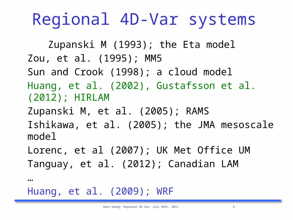
Regional 4D-Var systems

Zupanski M (1993); the Eta model

Zou, et al. (1995); MM5

Sun and Crook (1998); a cloud model

Huang, et al. (2002), Gustafsson et al. (2012); HIRLAM

Zupanski M, et al. (2005); RAMS

Ishikawa, et al. (2005); the JMA mesoscale model

Lorenc, et al (2007); UK Met Office UM

Tanguay, et al. (2012); Canadian LAM

…

Huang, et al. (2009); WRF


HIRLAM tests: 3D-Var vs 4D-Var Nils Gustafsson (SMHI)

• SMHI area, 22 km, 40 levels, HIRLAM 7.2, KF/RK, statistical bal-ance background constraint, reference system background error statis-tics (scaling 0.9), no ”large-scale mix”, 4 months, operational SMHI observations and boundaries

• 3D-Var with FGAT, 40 km increments, quadratic grid, incremental digital filter initialization

• 4D-Var, 6h assimilation window, Meteo-France simplified physics (vertical diffusion only), weak digital filter constraint, no explicit ini-tialization.

• One experiment with one outer loop iteration (60 km increments) and one experiment with two outer loop iterations (60 km and 40 km in-crements)


Nils Gustafsson


Nils Gustafsson


Nils Gustafsson


Nils Gustafsson




WRFDA is a Data Assimilation system built within the WRF software framework, used for

application in both research and operational environments….


• Summary

Outline


WRFDA Overview• Goal: Community WRF DA system for

• regional/global,

• research/operations, and

• deterministic/probabilistic applications.

• Techniques:

• 3D-Var

• 4D-Var (regional)

• Ensemble DA

• Hybrid Variational/Ensemble DA

• Model: WRF (ARW, NMM, Global)

• Observations: Conv. + Sat. + Radar (+Bogus)


www.mmm.ucar.edu/wrf/users/wrfda


Recent Tutorials at NCAR

1. WRFDA Overview

2. Observation Pre-processing

3. WRFDA System

4. WRFDA Set-up, Run

5. WRFDA Background Error Estimations

6. Radar Data

7. Satellite Data

8. WRF 4D-Var

9. WRF Hybrid Data Assimilation System

10. WRFDA Tools and Verification

11. Observation Sensitivity

Practice

1. obsproc

2. wrfda (3D-Var)

3. Single-ob tests

4. Gen_be

5. Radar

6. Radiance

7. 4D-Var

8. Hybrid

9. Advanced (optional)


Observing System Simulation Experiment (OSSE)2010-09-11-00 +6h precipitation

(IC and BC come from +12h forecast from 2010-09-10-12 NCEP FNL)


Sample the hourly precipitation obs. based on the NA METAR sta.(2066)

+ random error (<±1 mm)


4dvar

+6h total precipitation simulations

control

obs

4DVAR Control

“OBS”


A short list of 4D-Var issues

y observations, preprocessing, quality control

H new observation types, improving operators

R observational errors, tuning, correlated observational errors

xb improve models (an important part of DA!!)

B Statistical models, flow-dependent features

M and MT :Ź development and validity (and ensemble approaches)

Minimization algorithm Quasi Newton; Conjugate Gradient;

J =

1

2x0 - xb T B 1 x0 - xb 1

2yk H M k x0

TR 1 yk H M k x0

k


(WRFDA) Observations, y In-Situ:

- Surface (SYNOP, METAR, SHIP, BUOY).- Upper air (TEMP, PIBAL, AIREP, ACARS, TAMDAR).

• Remotely sensed retrievals:- Atmospheric Motion Vectors (geo/polar).- SATEM thickness.- Ground-based GPS Total Precipitable Water/Zenith Total Delay.- SSM/I oceanic surface wind speed and TPW.- Scatterometer oceanic surface winds.- Wind Profiler.- Radar radial velocities and reflectivities.- Satellite temperature/humidity/thickness profiles.- GPS refractivity (e.g. COSMIC).

Radiative Transfer (RTTOV or CRTM):– HIRS from NOAA-16, NOAA-17, NOAA-18, METOP-2– AMSU-A from NOAA-15, NOAA-16, NOAA-18, EOS-Aqua, METOP-2– AMSU-B from NOAA-15, NOAA-16, NOAA-17– MHS from NOAA-18, METOP-2– AIRS from EOS-Aqua– SSMIS from DMSP-16

• Bogus:

– TC bogus.

– Global bogus.


H maps variables from “model space” to “observation space” x y

– Interpolations from model grids to observation locations– Extrapolations using PBL schemes– Time integration using full NWP models (4D-Var in generalized form)

– Transformations of model variables (u, v, T, q, ps, etc.) to “indirect” ob-

servations (e.g. satellite radiance, radar radial winds, etc.)• Simple relations like PW, radial wind, refractivity, …• Radar reflectivity

• Radiative transfer models

• Precipitation using simple or complex models• …

!!! Need H, H and HT, not H-1 !!!

H - Observation operator

Z Z(T , IWC, LWC, RWC,SWC)

0

( )( ) ( , ( ))

dTRL B T z dz

dz


4D-Var


and use tendency information from observations.


of the analysis.





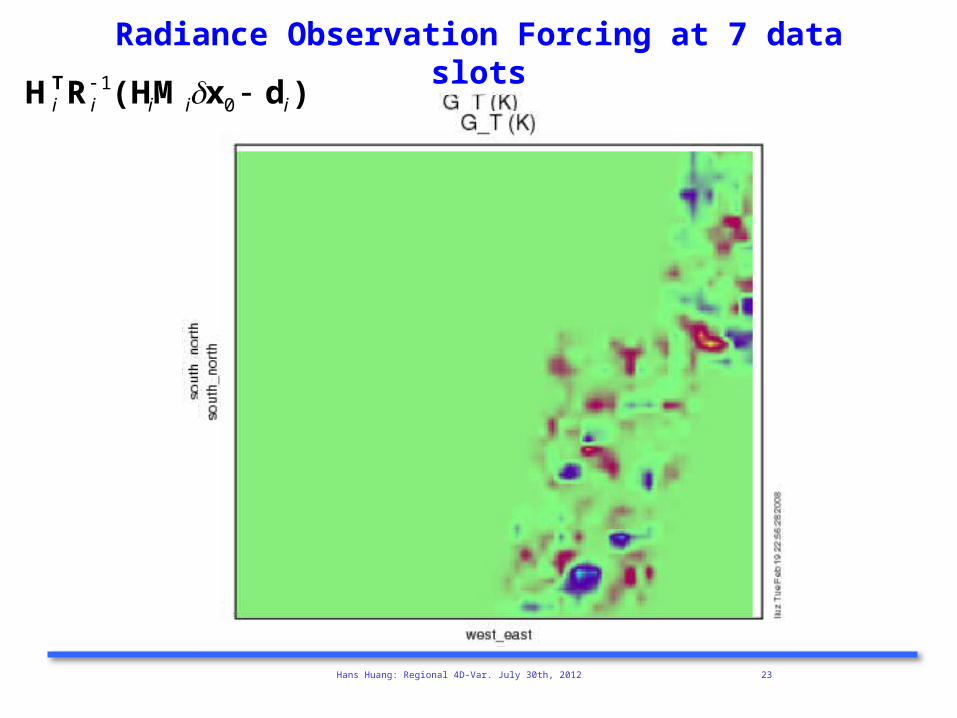
Radiance Observation Forcing at 7 data slots

H iTRi

1(HiM ix0 di)


A short list of 4D-Var issues

y observations, preprocessing, quality control

H new observation types, improving operators

R observational errors, tuning, correlated observational errors

xb improve models (an important part of DA!!)

B Statistical models, flow-dependent features

M and MT :Ź development and validity (and ensemble approaches)

Minimization algorithm Quasi Newton; Conjugate Gradient;

J =

1

2x0 - xb T B 1 x0 - xb 1

2yk H M k x0

TR 1 yk H M k x0

k


Assume background error covariance estimated by model perturbations x’ :

Two ways of defining x’:

The NMC-method (Parrish and Derber 1992):

where e.g. t2=24hr, t1=12hr forecasts…

…or ensemble perturbations (Fisher 2003):

Tuning via innovation vector statistics and/or variational methods.

Model-Based Estimation of Climatological Back-ground Errors

B (xb x t )(xb x t )T x'x'T

B x ' x 'T A(x t 2 x t1 )(x t 2 x t1 )T

B x ' x 'T C(x k x )(x k x )T


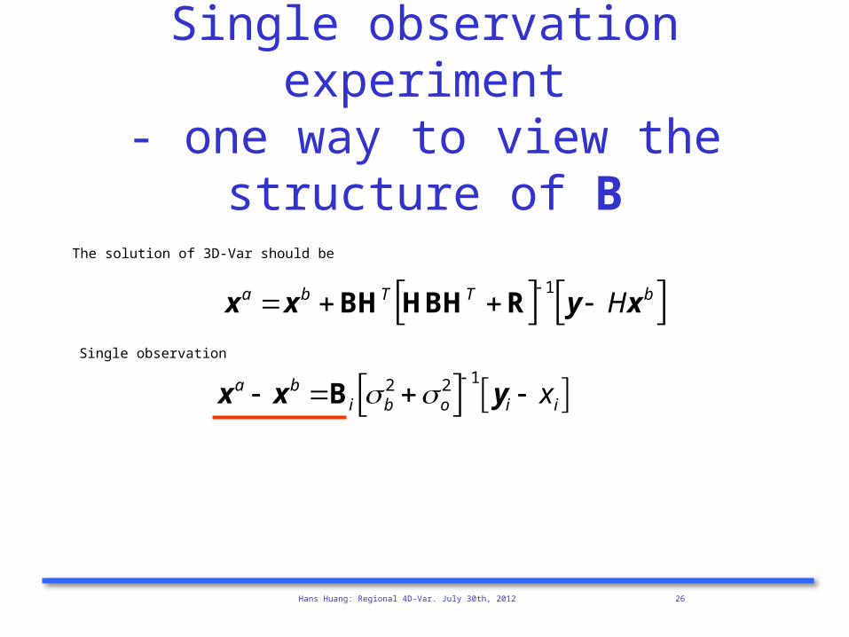
Single observation experiment- one way to view the structure of B

The solution of 3D-Var should be

xa xb BHT HBHT R 1y Hxb

Single observation

xa xb Bi b2 o

2 1yi x i


Pressure,

Temperature

Wind Speed,

Vector,

v-wind component.

Example of B 3D-Var response to a single ps observation


B from ensemble methodB from NMC method

Examples of B

T increments : T Observation (1 Deg , 0.001 error around 850 hPa)


Define preconditioned control variable v space transform

where U transform CAREFULLY chosen to satisfy Bo

= UUT .

Choose (at least assume) control variable components with uncorrelated errors:

where n~number pieces of independent information.

Incremental WRFDA Jb Preconditioning

Jb x t0 1

2x t0 xb t0 xg t0 T

Bo 1 x t0 xb t0 xg t0

x t0 Uv

Jb x t0 1

2vn

2

n


WRFDA Background Error Modeling

x t0 Uv UpUvUhv

Uh

: RF = Recursive Filter,

e.g. Purser et al 2003

Uv

: Vertical correlations

EOF Decomposition

Up

: Change of variable,

impose balance.



100

200

300

400

500

600

700

800

900

1000

0 100 200 300 400 500

Error correlation lengthscale (km)

Pre

ssur

e (h

Pa) u

v

T

p

q

x t0 Uv UpUvUhv

Uh



Uv


EOF Decomposition

Up


impose balance.



100

200

300

400

500

600

700

800

900

1000-0.5 -0.4 -0.3 -0.2 -0.1 0 0.1 0.2 0.3 0.4 0.5

Eigenvector Amplitude

Pre

ssu

re (

hP

a)

Mode 1Mode 2Mode 3Mode 4Mode 5

x t0 Uv UpUvUhv

Uh



Uv


EOF Decomposition

Up


impose balance.



Define control variables:

'

r' = q'/ qs Tb,qb, pb

u ' ' b ' '

Tu ' T ' Tb ' '

psu ' ps ' psb ' '

x t0 Uv UpUvUhv

Uh



Uv


EOF Decomposition

Up


impose balance.


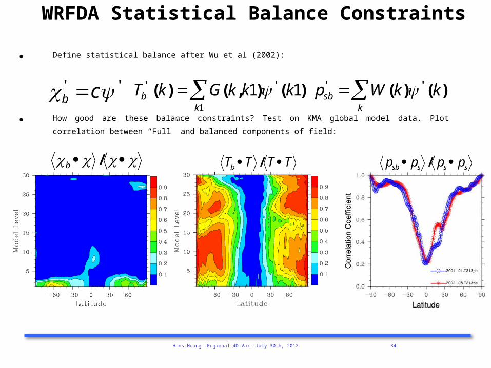
WRFDA Statistical Balance Constraints

• Define statistical balance after Wu et al (2002):

• How good are these balance constraints? Test on KMA global model data. Plot correlation between “Full” and balanced

components of field:

b /

Tb T / T T

psb ps / ps ps

b' c '

Tb' (k) G(k,k1) ' (k1)

k1

psb' W (k) ' (k)

k


Why 4D-Var?


and use tendency information from observations.


of the analysis.





Single observation experimentThe idea behind single ob tests:


xa xb BHT HBHT R 1y Hxb

Single observation

xa xb Bi b2 o

2 1yi x i

3D-Var 4D-Var: H HM; H HM; HT MTHT


xa xb BMTHT H MBMT HT R 1y HMxb

Single observation, solution at observation time

M xa xb MBMT i b

2 o2 1

yi x i


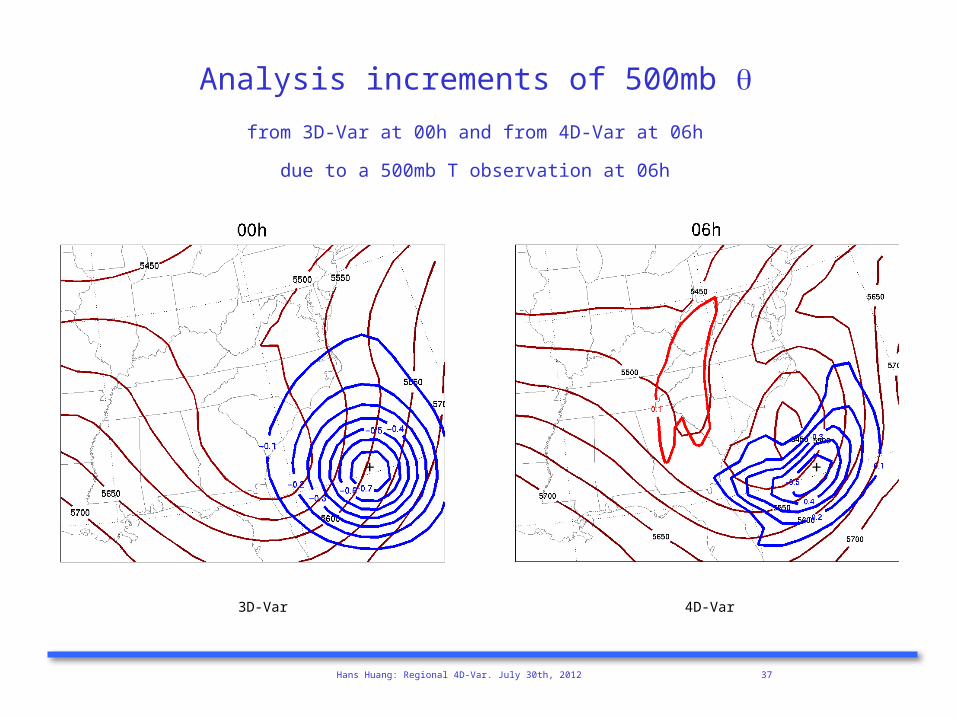
Analysis increments of 500mb q

from 3D-Var at 00h and from 4D-Var at 06h

due to a 500mb T observation at 06h

++

3D-Var 4D-Var


500mb q increments at 00,01,02,03,04,05,06h to a 500mb T ob at 06h

OBS+


500mb q difference at 00,01,02,03,04,05,06h from two nonlinear runs (one from background; one from 4D-Var)

OBS+


500mb q difference at 00,01,02,03,04,05,06h from two nonlinear runs (one from background; one from FGAT)

OBS+


Jb x0 12

x0 xb TB 1 x0 xb

Jo x0 1

2Hkx k yk T

R 1 Hkxk yk k1

K

Jc x0 df

2x N 2 xN 2

df T C 1 xN 2 xN 2df

df

2xN 2 fi

i0

N

xi

T

C 1 xN 2 fi

i0

N

xi

df

2hi

i0

N

xi

T

C 1 hi

i0

N

xi

where:

hi fi , if i N 2

1 fi , if i N 2

Control of noise: Jc


0

10000

20000

30000

40000

50000

60000

70000

80000

0 4 9 14 18 23 28 33 37 42

iterationsco

st f

unct

ion

JbJoJc

0

10000

20000

30000

40000

50000

60000

70000

80000

0 4 9 14 18 23 28 33 37 42

Iterations

cost

fu

nct

ion

Jb

Jo

Jc

Cost functions when minimize

J=Jb

+Jo

Cost functions when minimize

J=Jb

+Jo

+Jc

df

= 0.1


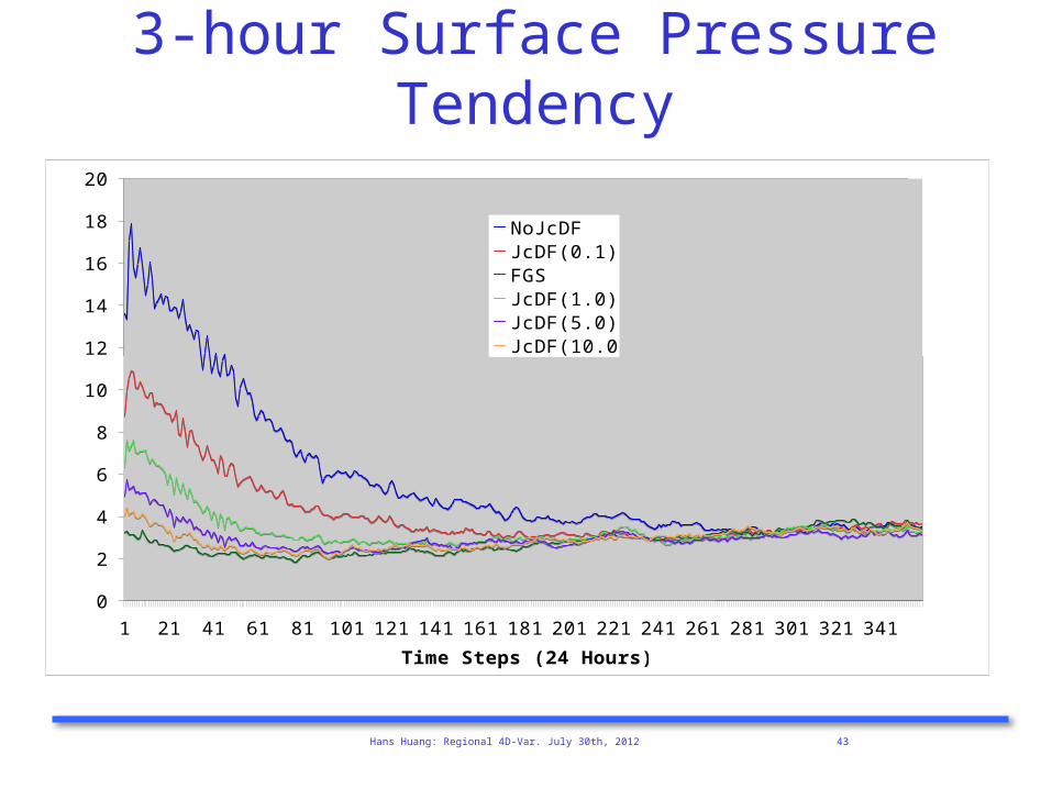
3-hour Surface Pressure Tendency

0

2

4

6

8

10

12

14

16

18

20

1 21 41 61 81 101 121 141 161 181 201 221 241 261 281 301 321 341

Time Steps (24 Hours)

DP

S/D

T

NoJcDFJcDF(0.1)FGSJcDF(1.0)JcDF(5.0)JcDF(10.0)


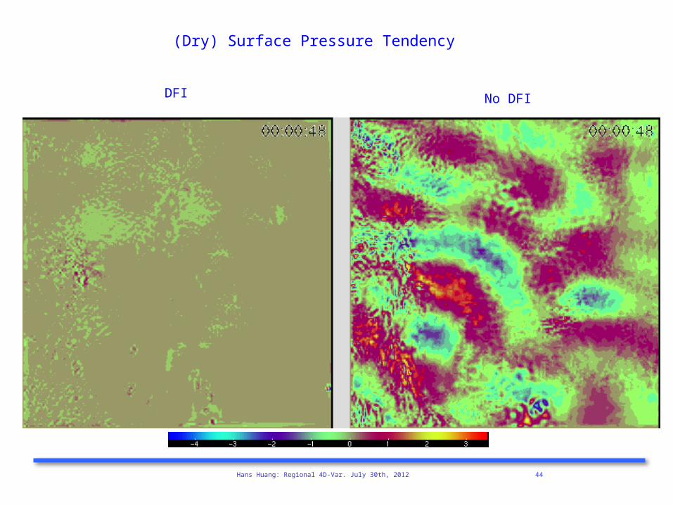
(Dry) Surface Pressure Tendency

DFI No DFI





• Summary

Outline


Issues specific to regional 4D-Var

Control of lateral boundaries.

Control of the large scales or coupling to a large scale model?

Mesoscale balances.


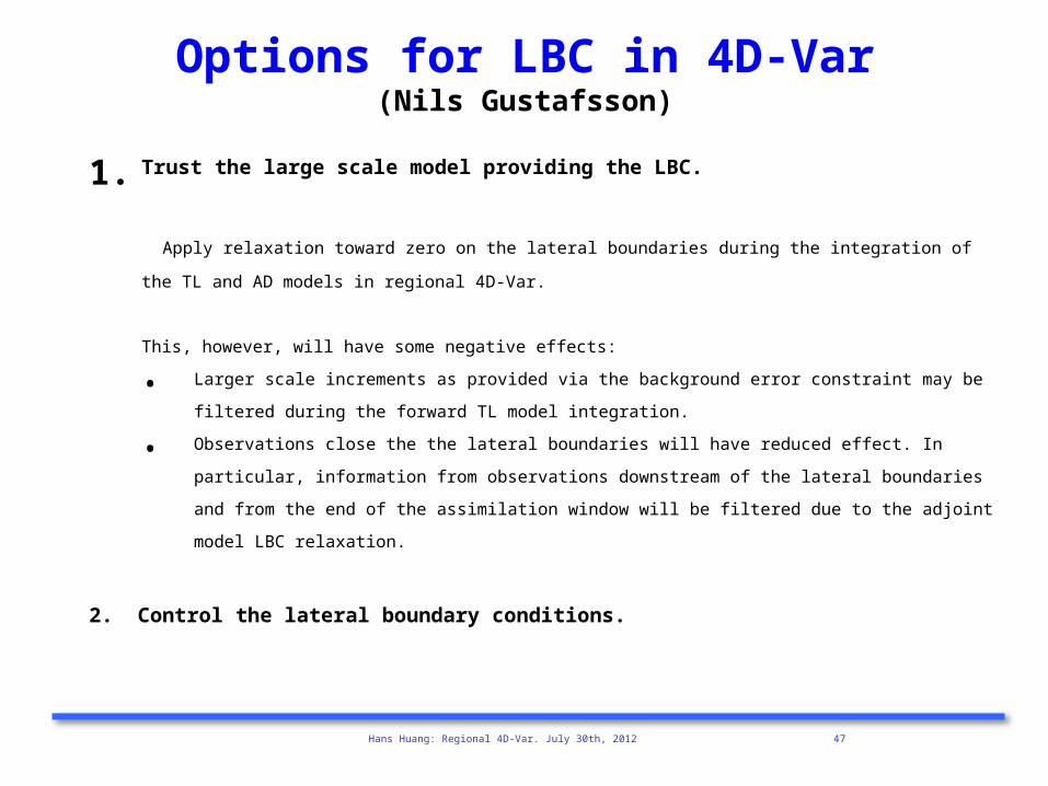
Options for LBC in 4D-Var(Nils Gustafsson)

1. Trust the large scale model providing the LBC.

Apply relaxation toward zero on the lateral boundaries during the integration of the TL and AD models in regional 4D-Var.

This, however, will have some negative effects:

• Larger scale increments as provided via the background error constraint may be filtered during the forward TL model

integration.

• Observations close the the lateral boundaries will have reduced effect. In particular, information from observations

downstream of the lateral boundaries and from the end of the assimilation window will be filtered due to the adjoint

model LBC relaxation.

2. Control the lateral boundary conditions.


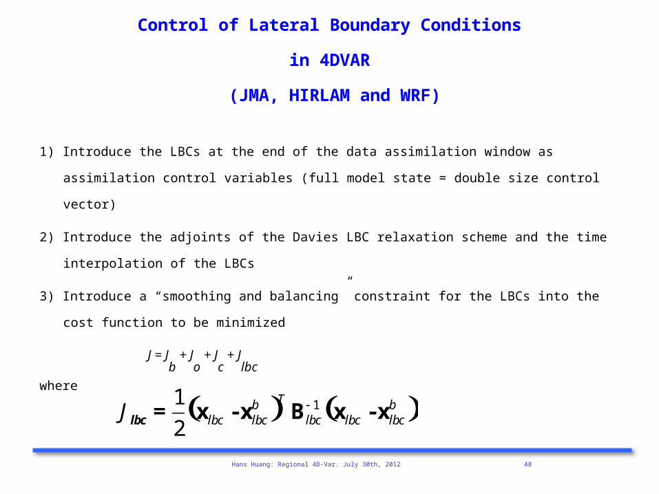
Control of Lateral Boundary Conditions

in 4DVAR

(JMA, HIRLAM and WRF)

1) Introduce the LBCs at the end of the data assimilation window as assimilation control variables (full model state =

double size control vector)

2) Introduce the adjoints of the Davies LBC relaxation scheme and the time interpolation of the LBCs

3) Introduce a “smoothing and balancing” constraint for the LBCs into the cost function to be minimized

J = Jb

+ Jo

+ Jc + J

lbc

where

J lbc =

1

2xlbc - xlbc

b T Blbc 1 xlbc - xlbc

b




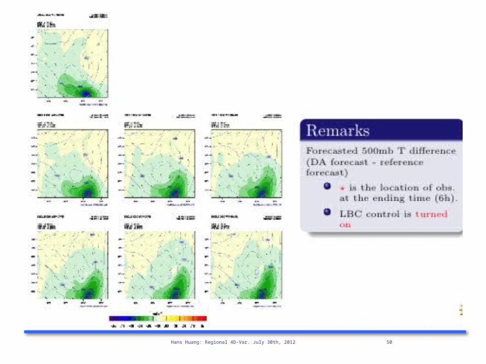
Problems with Control of LBC

• Double the control vector length• Pre-conditioning; LBC_0h and LBC_6h are

correlated• Relative weights for Jb and Jlbc??


Control of “larger” horizontal scales in re-gional 4D-Var

Per Dahlgren and Nils Gustafsson

• There are difficulties to handle larger horizontal scales in regional 4D-Var

• Observations inside a small domain may not provide information on larger horizontal scales

• The assimilation basis functions (via the background error constraint) may not represent larger scales properly .

• Possibilities in handling the larger horizontal scales:

- Via the LBC in the forecast model only; Depending on the cycle for refreshment of LBC, one may miss important

advection of information over the LBC

- Via ad hoc techniques for mixing in information from a large scale data assimilation (applied in HIRLAM).

- Via a large scale error constraint - Jls


A large scale error constraint - Jls

Add a large scale constraint Jls

to the regional 4D-Var cost function:

J = Jb

+ Jo

+ Jc + J

lbc + J

lswhere

• Has been tried in ALADIN 3D-Var with xls

being a global analysis from the same observation time. In this case one needs to, at

least in principle, use different observations for the global and regional assimilations

• Is being tried in HIRLAM 4D-Var with xls

being a global forecast valid at the start of the assimilation window.

For both applications one needs to check that (x-xb) and (x-xls

) are not too strongly correlated!

J ls =

1

2x - xls T Bls

1 x - xls


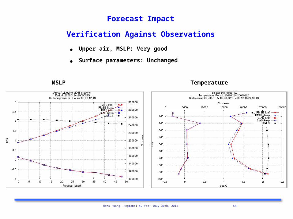
Forecast Impact

Verification Against Observations

MSLP Temperature

• Upper air, MSLP: Very good

• Surface parameters: Unchanged


• 4D-Var formulation and “why 4D-Var?”

• Why regional? (high resolution; regional observation network;…)

• The WRFDA approach: Jb; J

o; J

c

• Regional 4D-Var issues: Jlbc

, Jls

Summary

Date post:	18-Dec-2015
Category:	Documents
Upload:	kathleen-hensley
View:	216 times
Download:	0 times

Hans Huang: Regional 4D-Var. July 30th, 2012 1 Regional 4D-Var Hans Huang NCAR Acknowledgements:...

Documents