The Political Economy of Clean Coal A dissertation submitted in partial fulfillment of the requirements for the degree of Doctor of Philosophy at George Mason University By Hao Howard Wu Master of Electrical Engineering The University of Houston, 1998 Director: Charles K. Rowley Department of Economics Spring Semester 2010 George Mason University Fairfax, VA
Transcript
The Political Economy of Clean Coal
A dissertation submitted in partial fulfillment of the requirements for the degree of Doctor of Philosophy at George Mason University
By
Hao Howard Wu Master of Electrical Engineering The University of Houston, 1998
Director: Charles K. Rowley Department of Economics
Spring Semester 2010 George Mason University
Fairfax, VA
ii
Copyright 2010 Hao Howard Wu All Rights Reserved
iii
DEDICATION
This is dedicated to my loving wife Chau, whose unfailing support made all my dreams, including this one, come true.
iv
ACKNOWLEDGEMENTS
I would like to thank my committee members, Dr. Stephen Fuller and Dr. Bryan Caplan, for their timely and to-the-point comments which always kept me honest in my research. I would also like to especially thank my dissertation director, Dr. Charles Rowley, for tirelessly reviewing my drafts innumerable times and offering so many insightful comments. It is Dr. Rowley who encouraged me when I doubted myself, pushed me when I slowed down, and guided me when I veered astray; without his guidance this research project simply would not have come to fruition.
v
TABLE OF CONTENTS
Page
LIST OF TABLES............................................................................................................. vi LIST OF FIGURES .......................................................................................................... vii ABSTRACT..................................................................................................................... viii Chapter 1: Global Warming and CO2 – Setting the Scene ................................................. 1 Chapter 2: Sitting on a Huge Pile of Coal......................................................................... 12 Chapter 3: Dirtiest fuels of all – externalities of burning coal.......................................... 25 Chapter 4: Clean Coal Technologies ................................................................................ 57 Chapter 5: Obstacles to the Large-scale Deployment of Clean Coal Technologies ......... 79 Chapter 6: The Political Economy of Clean Coal............................................................. 96 Chapter 7: Conclusions ................................................................................................... 129 Appendix: Calculation of Full Costs of Electricity for IGCC and PC plants ................. 142 REFERENCES ............................................................................................................... 146
vi
LIST OF TABLES
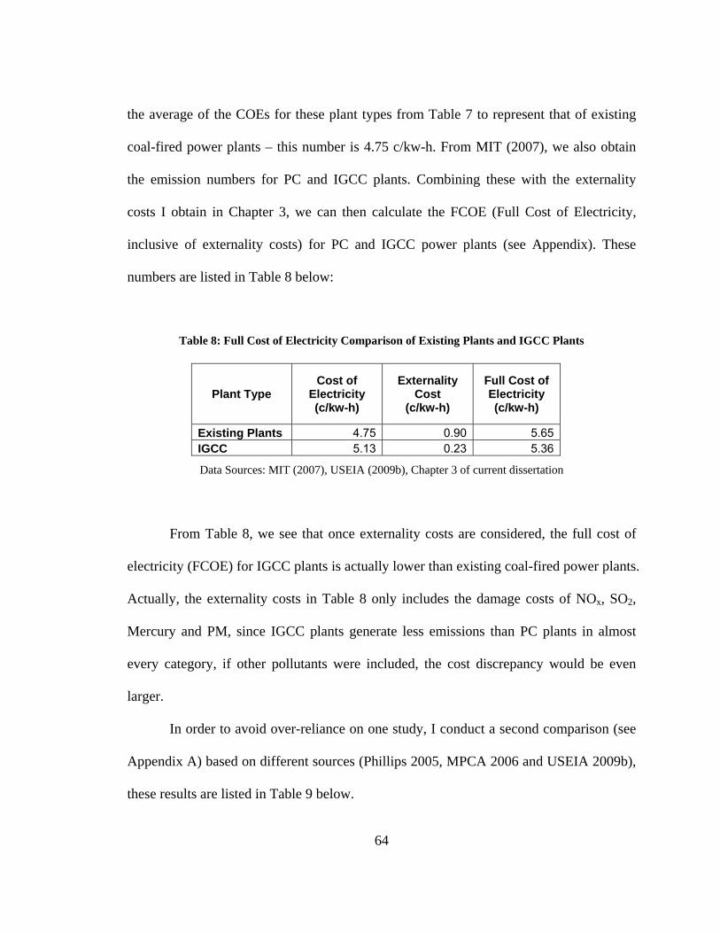
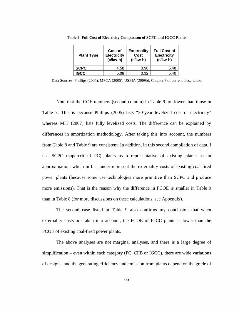
Table Page Table 1: Major Harmful Materials from Coal Emission................................................... 29 Table 2: Major Pollutants Emitted by Coal-fired Power Plants ....................................... 30 Table 3: Gross Annual Damages of NOx, SO2 and PM.................................................... 34 Table 4: Total costs of Arsenic, Chromium and Cadmium .............................................. 36 Table 5: Gross Annual Damages from Coal-generated Pollutants ................................... 42 Table 6: Descriptive Statistics of All Coal-fired Power Plants in the United States ........ 61 Table 7: Levelized Cost of Electricity for Each Plant Type ............................................. 63 Table 8: Full Cost of Electricity Comparison of Existing Plants and IGCC Plants ......... 64 Table 9: Full Cost of Electricity Comparison of SCPC and IGCC Plants........................ 65 Table 10: Levelized Cost of Electricity for Each Plant Type When Equipped
With CO2 Capture ..................................................................................................... 72 Table 11: Relative Cost of Electricity Comparison of PC and IGCC Plants When
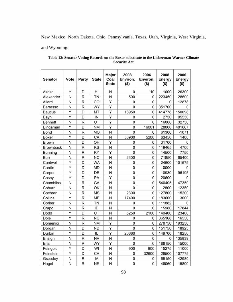
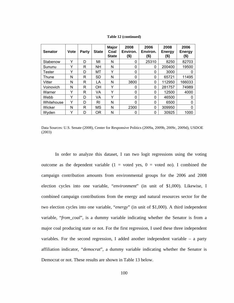
Equipped With CO2 Capture From Various Studies................................................. 73 Table 12: Senator Voting Records on the Boxer substitute to the Lieberman-
Warner Climate Security Act.................................................................................... 98 Table 13: Multivariate Logit Regression Results of Senator Voting Data ..................... 101 Table 14. Plaintiffs in Massachusetts v. EPA that received money from The
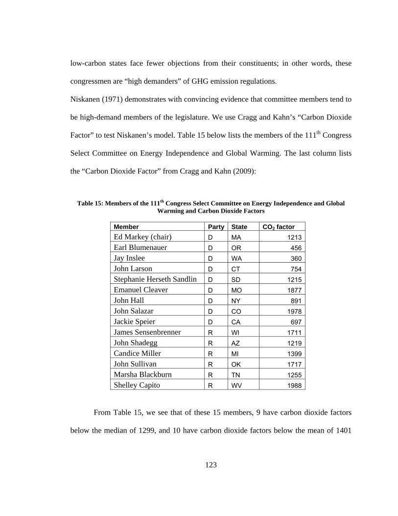
Energy Foundation.................................................................................................. 119 Table 15: Members of the 111th Congress Select Committee on Energy
Independence and Global Warming and Carbon Dioxide Factors ......................... 123 Table 16: Externality Costs of Existing Coal-fired Power Plants................................... 142 Table 17: Projected Externality Costs of IGCC Plants based on MIT (2007) and
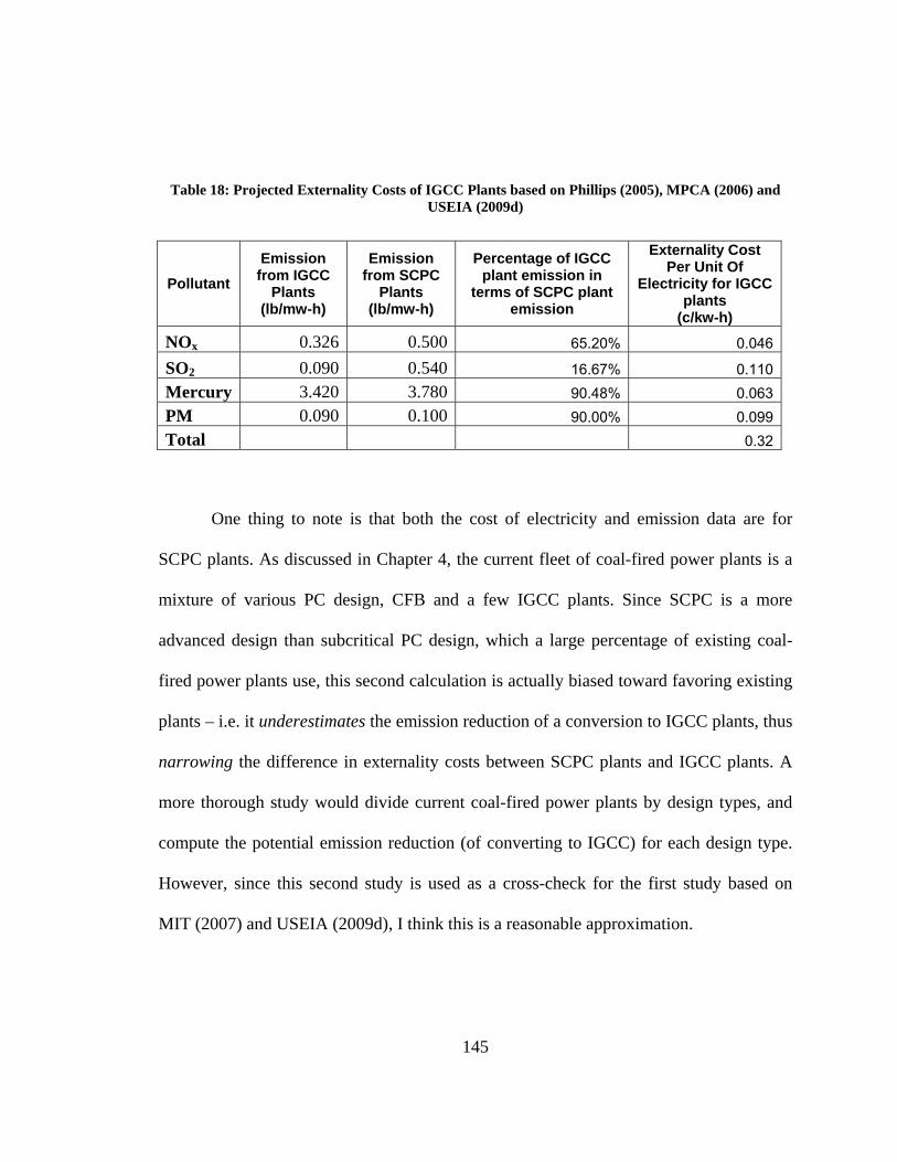
USEIA (2009d) ....................................................................................................... 144 Table 18: Projected Externality Costs of IGCC Plants based on Phillips (2005),
MPCA (2006) and USEIA (2009d) ........................................................................ 145
vii
LIST OF FIGURES
Figure Page Figure 1: Monthly Average Carbon Dioxide Concentration .............................................. 2 Figure 2: Global Land-Ocean Temperature Index.............................................................. 3 Figure 3: Global Surface and Lower Troposphere Monthly Mean Anomalies
Relative to the 1979-1998 Mean Temperature. .......................................................... 5 Figure 4: World Energy Consumption by Fuel Type, 2006 ............................................. 17 Figure 5: Net Generation Shares by Energy Source in the U.S., Year-to-Date
through February, 2009............................................................................................. 18 Figure 6: World Marketed Energy Use by Fuel Type, 1980-2030 ................................... 19 Figure 7: Summary of Estimates of Demand Price Elasticities for Fossil Fuels .............. 20 Figure 8: Global primary energy supply........................................................................... 23 Figure 9: Stock and Flow Externalities............................................................................. 44 Figure 10: Externality Comparison between Criteria Pollutants and Carbon
Dioxide...................................................................................................................... 45 Figure 11: The probability density functions of the 103 estimates of the marginal
costs of carbon dioxide emissions (gray) and the composite probability density function (black). ........................................................................................... 47
Figure 12: The composite probability density function of the marginal costs of carbon dioxide using author weights (light gray), quality weights (black), and quality weights including peer-reviewed studies only (dark gray). ................... 47
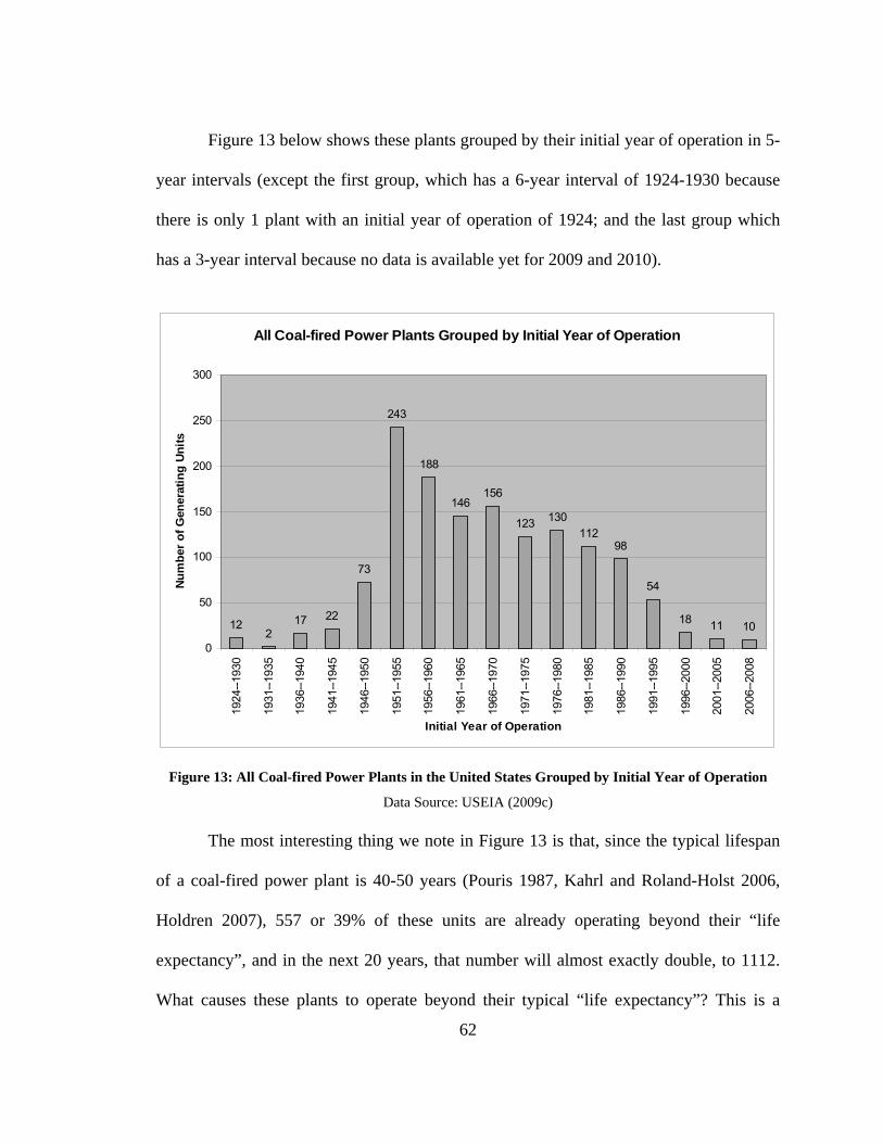
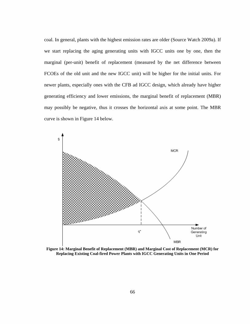
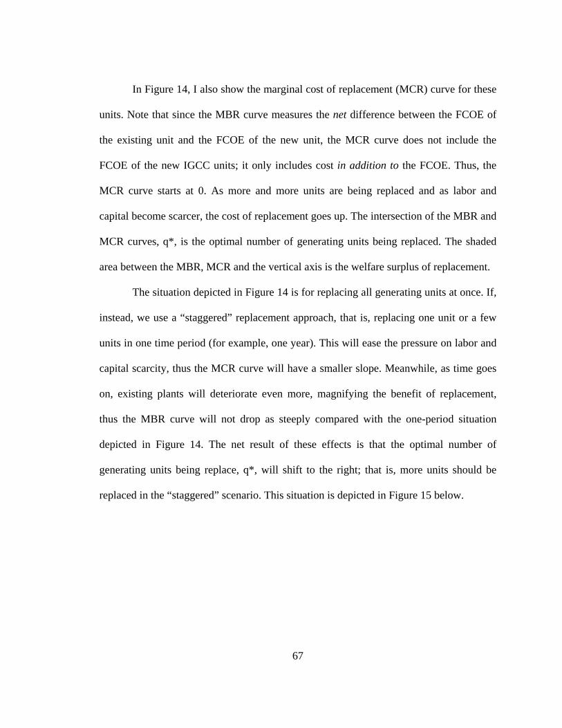
Figure 13: All Coal-fired Power Plants in the United States Grouped by Initial Year of Operation ..................................................................................................... 62
Figure 14: Marginal Benefit of Replacement (MBR) and Marginal Cost of Replacement (MCR) for Replacing Existing Coal-fired Power Plants with IGCC Generating Units in One Period ..................................................................... 66
Figure 15: Marginal Benefit of Replacement (MBR) and Marginal Cost of Replacement (MCR) for Replacing Existing Coal-fired Power Plants with IGCC Generating Units, Staggered Scenario............................................................ 68
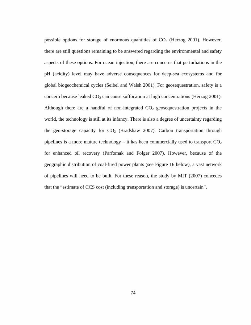
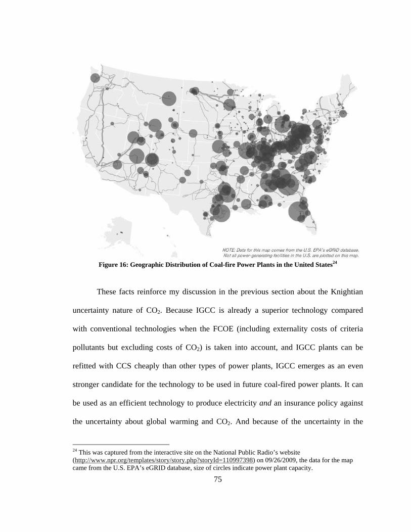
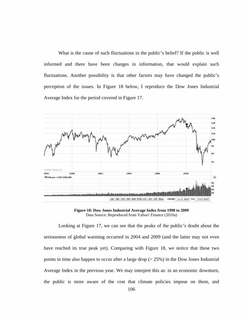
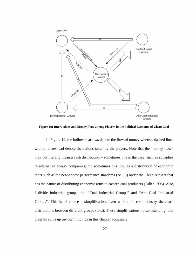
Figure 16: Geographic Distribution of Coal-fire Power Plants in the United States........ 75 Figure 17: Global Warming Survey Results, 1998 – 2009............................................. 105 Figure 18: Dow Jones Industrial Average Index from 1998 to 2009 ............................. 106 Figure 19: Interactions and Money Flow among Players in the Political Economy
of Clean Coal .......................................................................................................... 127
ABSTRACT
THE POLITICAL ECONOMY OF CLEAN COAL Hao Howard Wu, Ph.D. George Mason University, 2010 Dissertation Director: Dr. Charles K. Rowley This dissertation investigates the nature of the political economy of Clean Coal. It begins
by reviewing the literature of global warming and the current usage of coal in the United
States and throughout the world. It examines the externality costs from burning coal, and
reviews Clean Coal technologies. Based on the comparison of total costs of generating
electricity between Clean Coal and conventional technologies, it concludes that Clean
Coal technologies are more economically efficient. Based on marginal net benefit
analysis, it proposes that the optimal approach to deploy Clean Coal technologies is to
gradually replace existing facilities with ones equipped with Clean Coal technologies. It
identifies two obstacles that prevent the large-scale deployment of Clean Coal
technologies: the New Source Review program under the Clean Air Act and the
regulation of greenhouse gases. It then uses a public choice framework to find that the
rent-seeking activities of interest groups are the forces that created these obstacles. It
concludes by making public choice compatible recommendations for policy reform that
would one day make Clean Coal a reality.
1
Chapter 1: Global Warming and CO2 – Setting the Scene 1. “King Coal” – Fuel for Economic Growth or Cancer to Society?
Humans have used coal for thousands of years (California Energy Commission 2002).
Since the industrial revolution, coal has played a vital role in supplying the energy
needed to fuel the economic growth of our society (Wrigley 1962). In recent years,
however, coal has increasingly been vilified, portrayed by some not as the fuel that
propels economic growth, but as a “cancer” to society. Consider, for example, articles
with titles such as “Killing King Coal” (Martelle 2009) and “The Enemy of the Human
Race” (Hansen 2009) have regularly appeared in pro-environment publications such as
the Sierra magazine, and former Vice President and environmental activist Al Gore has
urged young people to engage in “civil disobedience” against coal (Nichols 2008).
It has long been recognized that burning coal generates various pollutants, such as
nitrogen oxides, sulfur dioxide, particulate matter, mercury, etc. However, the recent
surge of vilification of coal is linked to one particular “pollutant” from coal – carbon
dioxide (CO2). The reason for this is that many believe that CO2 has the potential to
contribute to global warming. Related to this, the debate on Clean Coal has also been
heating up: proponents think that it has a bright future, while others, such as Al Gore,
decry and mock it as “nonexistent”. Indeed, even the term “Clean Coal” seems to be a
source of confusion – some equate it with carbon capture and sequestration (CCS) while
1
others use it as an umbrella term that encompasses modern abatement technologies (I will
give a clear definition of “Clean Coal” and discuss related issues in more detail in
Chapter 4).
In this dissertation, I set out to understand the analytical history and political
economy of Clean Coal. There are several concrete questions I ask at the end of this
chapter. But for the moment, because global warming and CO2 are at the center of the
debate on Clean Coal, I shall take a brief detour to review the scientific literature of
global warming and CO2.
2. A Brief Detour – Global Warming and CO2
The “Greenhouse Effect” was first hypothesized by the French mathematician and
physicist Jean Baptiste Joseph Fourier in 1824, who discovered that certain gases have
the property of trapping long-wave radiations. Later work by the Swedish physicist and
chemist Svante August Arrhenius in 1896 formalized the theory that changes in the levels
of atmospheric carbon dioxide could substantially alter the surface temperature through
the greenhouse effect. In the 1930s the English engineer Guy Stewart Callendar expanded
upon the works of Arrhenius and others and concluded that an increase in atmospheric
CO2, induced by human activity, could lead to global warming – this is what became to
known as anthropogenic global warming (Ramanathan 1988). Because of this, CO2 is
considered to be a greenhouse gas (GHG).
A great deal of empirical work has been undertaken to measure atmospheric CO2
concentration and global temperature variations. Atmospheric CO2 concentration is
2
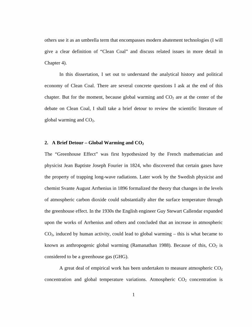
directly measurable; its increase has been verified. Measurements indicate that its mean
annual concentration has increased steadily during the period from 1959 to 2004 – from
315.98 parts per million by volume (ppmv) of dry air to 377.38 ppmv (US NOAA 2009),
a 19.4% increase. This result is reproduced in Figure 1.
Figure 1: Monthly Average Carbon Dioxide Concentration Data Source: US NOAA (2008)
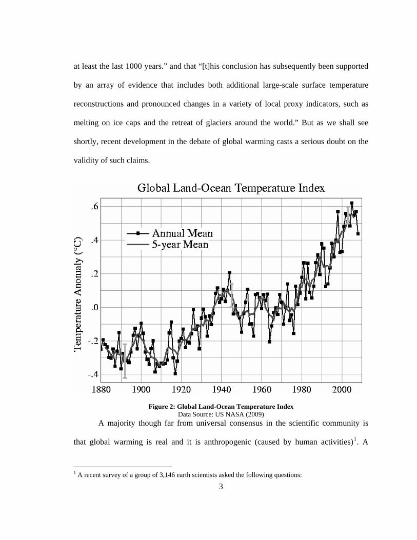
Observation data of global earth surface temperature also show a warming trend:
it increased by about 0.74 °C (1.33 °F) during the last 100 years (US NASA 2009). This
result is reproduced in Figure 2 below. The National Academies (2006) also report that
“… the late 20th century warmth in the Northern Hemisphere was unprecedented during
3
at least the last 1000 years.” and that “[t]his conclusion has subsequently been supported
by an array of evidence that includes both additional large-scale surface temperature
reconstructions and pronounced changes in a variety of local proxy indicators, such as
melting on ice caps and the retreat of glaciers around the world.” But as we shall see
shortly, recent development in the debate of global warming casts a serious doubt on the
validity of such claims.
Figure 2: Global Land-Ocean Temperature Index Data Source: US NASA (2009)
A majority though far from universal consensus in the scientific community is
that global warming is real and it is anthropogenic (caused by human activities)1. A
1 A recent survey of a group of 3,146 earth scientists asked the following questions:
4
sizable yet growing minority of scientists challenge this position. For example, in a report
to the Nongovernment International Panel on Climate Change, American atmospheric
physicists S. Fred Singer (2008) and other scientists use results from latest climatologic
research to demonstrate that most modern warming is due to natural causes and not
human activities, and that the effects of human CO2 emissions are benign. Other
scientists also raise serious questions about the extent, cause and effect of global warming.
The following is a partial list of these arguments:
1. The extent of global warming may not be as large as perceived (Soon and
Baliunas, 2003)
2. A large portion of the recent warming trend may be part of longer climate cycle of
the earth (Balling 2005)
3. Other effect, such as the El Niño phenomenon (ibid) and solar variability
(Baliunas 2005) may have contributed to global warming.
4. Limitations in computer modeling makes climate change predications unreliable
(Soon, et. al. 2001)
Some scientists also point out that the unusually large warming “spike” in 1998
may be caused by unprecedented El Niño activities (Michaels 2009). Indeed, more recent
observation data suggest that there has been relative global “cooling” since 1998 (see
Figure 3 below). 1) Have mean global temperatures risen compared to pre-1800s levels? 2) Has human activity been a significant factor in changing mean global temperatures? About 90 percent of the scientists agreed with the first question and 82 percent the second. See Science Daily (Jan. 21, 2009) Scientists Agree Human-induced Global Warming Is Real, Survey Says (website: http://www.sciencedaily.com/releases/2009/01/090119210532.htm), the original survey was published in the journal Eos, Transactions by American Geophysical Union on Jan. 19, 2009
5
Figure 3: Global Surface and Lower Troposphere Monthly Mean Anomalies Relative to the 1979-1998 Mean Temperature.
Data from GISS, HadCRU, RSS, and UAH ranging from January 1979 to February 2008 (reproduced from Hausfather (2008))
As of this writing, the debate of global warming has taken another dramatic turn –
now even the authenticity of the data supporting the anthropogenic global warming
hypothesis has been called into question. In November, 2009, the leaked emails from one
of the institutions at the center of studying climate change – the Climate Research Unit
(CRU) of University of East Anglia (a second rate British university which nonetheless
acts as a repository of atmospheric temperature data) suggest that leading researchers at
this institution have manipulated the data to exaggerate the upward temperature trends
(Hickman and Randerson 2009). In a more recently published correspondence with the
person who is at the center of this controversy, the director of the CRU, Phil Jones, Jones
admitted that a number of warming periods occurred in history, including the one that is
6
cited most often as the evidence of anthropogenic global warming – the period from 1975
to 2009, are “not significantly different from each other” (BBC News 2010). Jones also
admitted that that has been a cooling trend from January 2002 to the present (February
2010), although he claims that this is not statistically significant. But the most revealing
concession from Jones is the following statement: “There is still much that needs to be
undertaken to reduce uncertainties [in the study of global warming]” (ibid).
I do not wish to delve further into the details of this debate, as that is beyond the
scope of this dissertation and not the focus of my research. I conclude that there are still a
lot of uncertainties regarding anthropogenic global warming – a point upon which even
its most ardent believers agree.
Now let us turn to the economic aspects of global warming. The net economic
effect of global warming is not universally negative. For example, within a certain range,
global warming has positive economic effect on agriculture (Mendelsohn et. al. 1994).
Even one of the staunchest advocates for global climate control Nicholas Stern concedes
that at the lower end (increase of 2 or 3°C) climate change may have positive effects for
countries in cold regions (Stern 2007). At the high end, the net economic effect of global
warming may well be negative – intuitively, in the highly unlikely event that global
warming is so severe as to make our planet inhospitable, certainly that outcome would be
a net cost to society. Therefore the issue rests on the question: how severe will global
warming be? Pooley (2008) asserts that “economists overwhelmingly agree that business
as usual will lead to greatly increased societal costs as the impacts of climate change set
in”. However, some economists also argue that even in the face of high degree of global
7
warming, human biophysical adaptations will be a factor mitigating against major impact
(Davis 2005).
It is important to realize that even if anthropogenic global warming is real, if we
were to enact some regulation to control it, we must take the economic cost and benefit of
such regulation into consideration. For example, if the global warming is real, but its
extent is not very great, its damages may be limited (in fact the net effect could be
beneficial), then it makes no economic sense to implement measures that cost more than
the damages to mitigate it. Similarly, if human activities that produce CO2 and other
GHG only play a limited role in causing global warming, which is mainly determined by
longer climate cycles or influenced by solar variability, then restricting these activities
may not reduce global warming very much, whereas the economic cost of reducing these
activities may be enormous.
Yet global collective action on climate control is already a political reality – the
European Union has already implemented an Emission Trading Scheme (ETS) in 2005
(European Commission 2008). In the U.S., a cap-and-trade program, Regional
Greenhouse Gas Initiative (RGGI), supported by 10 northeastern states also went into
effect in 2008 (RGGI 2009). Because coal-fired power plants are a major source of CO2
emissions, climate regulations inevitably will affect – either facilitate or retard – the
adoption of Clean Coal technologies. This is a topic that I shall return to in later chapters,
but for now, I conclude this brief detour on global warming and CO2 by remarking that
despite the uncertainties about global warming and the role that CO2 plays in causing it,
8
climate regulations are a political reality at the center of the political economy of Clean
Coal.
3. Research Methodology and Agenda
Having briefly reviewed the literature on global warming and CO2, I now return to the
focus of my study: the political economy of Clean Coal.
There are two aspects of my study: first, the economic aspect of coal and Clean Coal
technologies. For this, my methodology is grounded in economic efficiency analysis. For
example, when I inquire about the nature of Clean Coal technologies, I am most
interested in whether they are economically efficient – that is, whether the marginal
social benefit of deploying Clean Coal technologies equals the marginal social cost; I am
less interested in the engineering details.
The second aspect of my study is the political aspect of Clean Coal related
activities by various players in this political “game”. For this, my methodology is
grounded in public choice analysis. In particular, one of the premises in public choice is
that individuals’ political activities – just as their economic activities – are motivated by
self-interest; consequently, I am especially interested in examining the incentives and the
constraints of the players in the political game; as such, I pay little attention to what
people say (talk is cheap), but pay a great deal of attention to what they do.
A study of the political economy of Clean Coal is a major undertaking; one
cannot hope to do it alone. There have been numerous studies on topics related to my
inquiry, for example, cost estimates of coal-generated pollutants, economic analysis of
9
Clean Coal technologies, public choice studies of coal related environmental regulations,
etc. I rely on this literature, especially peer-reviewed articles. I critically review and
synthesize the relevant findings from this vast literature. Additionally, I also conduct my
own studies, sometimes using the same methodologies used in other studies but applying
them to different specific problems, sometimes conducting economic efficiency and
econometric analyses of my own.
In my dissertation, I set out to answer the following questions:
Question #1: Is it realistic to expect coal use to be reduced significantly or
eliminated altogether in the near future?
As I mentioned in the beginning paragraph of this chapter, there are individuals,
particularly environmental activists, most noticeably Al Gore, who are trying to wipe out
the coal industry in the United States. But is it realistic to expect coal to be “phased out”
in the foreseeable future? Indeed, if coal is phased out entirely, the debate on Clean Coal
becomes moot. Thus, this is the first question I must answer.
Question #2: How dirty is coal – in other words, what is the economic cost from
coal-generated pollutants?
There are several cost estimates of a particular pollutant or pollutants from coal,
but to my knowledge, there is no estimate of the economic cost of all the major coal-
generated pollutants. I aim to estimate the damage cost of the sum total of all the major
coal-generated pollutants. This estimate is crucial in evaluating the economic efficiency
of Clean Coal technologies.
Question #3: What is the nature of the uncertainty regarding CO2?
10
CO2 is at the center of GHG regulations. However, as I pointed out earlier, there
are still uncertainties about the extent, cause and effect of global warming, and there is
uncertainty about the role CO2 plays in causing it. But there is always uncertainty about
any pollutant – cost estimates of pollutants can vary by orders of magnitude. Is the degree
of uncertainty about CO2 the same as or different from the degree of uncertainty about
other pollutants? The answer to this question is very important in evaluating GHG
regulations.
Question #4: Are “Clean Coal technologies” more economically efficient
compared with conventional technologies?
Most comparisons of Clean Coal technologies with conventional technologies
focus on the costs in producing electricity but ignore externality costs – costs from
pollutants borne by people other than the owners and operators of coal-fired power plants.
Because Clean Coal technologies have the potential to reduce emissions, I make the
comparison based on full costs (inclusive of externality costs) in producing electricity.
This is the most meaningful comparison, and by focusing on it I provide a new
perspective in this line of research.
Question #5: If Clean Coal technologies are economically more efficient than
conventional technologies, what is the optimal approach to large-scale deployment of
Clean Coal technologies?
This question is contingent on the answer to the previous question. Given that the
answer to the previous question turns out to be positive, then I sketch an optimal
11
approach to large-scale deployment of Clean Coal technologies based on economic
efficiency analysis.
Question #6: If in reality, the level of utilization of Clean Coal technologies is
suboptimal, what are the obstacles that prevented the optimal level from being achieved?
This question is contingent on the findings of current utilization level of Clean Coal
technologies and the answers to the previous two questions. Given that Clean Coal
technologies turn out to be economically more efficient than conventional technologies,
and that the utilization level of Clean Coal technologies turns out to be suboptimal, then I
seek out and identify the political obstacles that are primarily responsible for such a
suboptimal outcome. To this end, I deploy public choice analysis.
Finally, after answering all these questions, I outline public choice compatible
policy reform recommendations designed to remove the political obstacles and to move
toward a world with Clean Coal, a world in which coal can be used most efficiently to
further the economic efficiency of society.
12
Chapter 2: Sitting on a Huge Pile of Coal The U.S., like China and India, sits on a huge pile of coal …
– John B. Heywood, “Growing Pains - Transitioning to a Sustainable Energy Economy”
MIT World Lecture, November 1, 2006 1. Brief History of Coal Coal is formed from plant remains from the Carboniferous Period (the word
“Carboniferous” literally means “coal bearing” in Latin) of the late Paleozoic Era about
354 to 290 million years ago (Prothero & Dott 2003). It is composed mostly of carbon
and hydrogen based organic compounds, but it also contains small quantities of other
elements such as nitrogen, sulfur and mercury. The plants from whose remains coal is
formed absorbed carbon dioxide (CO2) from the atmosphere and transformed it into
organic matters through photosynthesis. Thus, in essence, coal, like other fossil fuels such
as petroleum and natural gas, is sequestered carbon from earlier geological times.
Humans have long recognized coal as an energy source. The Chinese may have
used it as early as 3000 years ago (California Energy Commission 2002). When James
Watt improved the steam engine in the 1770s, coal was used to heat up the water in the
boiler to generate the steam; when Thomas Edison invented the electrical generator in the
1870s to provide electricity for another of his inventions, the light bulb, his choice of fuel
was also coal. By some accounts, coal was “[t]he decisive technological change which
13
freed so many industries from dependence upon organic raw materials” (Wrigley 1962).
The increasingly widespread use of coal was driven by both increased demand for energy
and technological innovation in mining (Clark and Jacks 2007). We conclude that coal is
the energy source that fueled the industrial revolution.
2. Estimates of Coal Reserves
Coal is the most abundant fossil fuel and readily usable energy source: according to the
most recent U.S. Energy Information Administration report (USEIA 2008a), total
recoverable reserves of coal around the world are estimated at 930 billion tons. To
compare different fossil fuels, it is necessary to use a common unit. The “heat content”
(energy content) is usually used for this purpose. The grade of coal can vary substantially,
resulting in different heat contents; nevertheless, we can use an average value estimate
the energy content of the total coal reserves in the world. According to the USEIA
(2008b), the average heat content of coal used in electricity generation in the U.S. is
19.78 million Btu (British Thermal Unit) per ton, thus the world’s total coal reserves
translate to a total heat content of 18,395 quadrillion Btu. In comparison, using the two
aforementioned sources, the world’s total natural gas reserves are estimated at 6,186
trillion cubic feet, or 6,372 quadrillion Btu; the world’s total oil reserves are estimated at
1,332 billion barrels, or 8,258 quadrillion Btu. In other words, the energy content of the
world’s coal reserves is about 25% greater than that of the world’s natural gas and oil
reserves combined.
14
Anecdotally, the United States has 250 years of coal reserve. President George W.
Bush once famously (and apparently mistakenly, by a factor of 1 million) said that we
have “250 million years of coal?”2 The Energy Information Agency (EIA) of the U.S.
Department of Energy website also states that there is “enough coal to last approximately
225 years at today's level of use” (USEIA 2008c). However, such notion is not without
dispute. A research by Molnia et. al. (1999) shows that such estimates may be grossly
overestimated. Molnia et. al. used three definitions to distinguish between “original coal”
(total coal deposits) vs. “recoverable resource” (technologically extractable coal) and
“economically recoverable” coal:
Available coal ≡ original coal – areas already mined – land-use restrictions
– technologic considerations
Recoverable resource ≡ coal available for mining – mining loses –
By their estimates, in some regions, the percentage of original coal that is
available varies from 48% to 60%, while the percentage of original coal that is
economically recoverable may be as little as 11%.
Molnia et. al.’s research highlights the uncertainties in fossil fuel reserve
estimates and the many technological and economic constraints on these resources. But
2 Source: President Discusses Strengthening Social Security in Washington, D.C., Official website of the White House (http://georgewbush-whitehouse.archives.gov/news/releases/2005/06/20050608-3.html, retrieved: 05/25/2009)
15
their research takes the technological and economic constraints as exogenous. As
technologies advance, more coal will be extractable. Even more importantly, increased
demand for a natural resource spurred by economic growth will exert an upward pressure
on the price of that resource. This demand pressure makes resources that were previously
too costly economically attainable. Indeed, economic conditions often play a more
important role than technological advances in determining the use and availability of
natural resources: historical evidence suggests that the expanded coal output in the
Industrial Revolution was mainly a result of increased demand rather than technological
innovations in mining (Clark and Jacks 2008). Furthermore, as Krautkreamer (2005)
argues, price increases because of increasing scarcity will also trigger a variety of
responses such as substitutions with other resources, resource-saving technologies,
methods for recovering resources and cost reduction of using lower-quality reserves, etc.
All these responses will in turn ameliorate the scarcity. Because of these factors, we
believe that Molnia et. al. have underestimated total coal reserves in the United States.
Molnia et. al.’s estimates also remind us of the gloomy prediction made by “The
Club of Rome” that the world would run out of oil before 1992 (Meadows, Randers and
Meadows, 1972[2004]). In reality, we are well into the 21st century, such resource
depletion not only has not happened, it is nowhere nearly in sight.
From these researches we make the following conclusions: First, there is great
uncertainty in estimates of available natural resources; history suggests that we have
always tended to underestimate natural resource reserves in the past. Secondly, there are
two aspects regarding the abundance of nonrenewable resources. On one hand, the
16
amounts of nonrenewable resources are finite; eventually they will run out. This is
especially true in the case of fossil fuels as they are fossilized living organisms in earlier
geological times3. It is conceivable that as technologies advance, we may be able to
exploit inorganic minerals from the moon, other planets or even other celestial bodies.
But so far scientific inquiries have not produced any evidence of extraterrestrial life
forms, the possibility that we will find and utilize other sources of fossil fuels than from
our own planet is exceedingly remote. On the other hand, the important issue is not
whether these resources will run out, but when they will run out. In other words, we must
put it within the timeframe of our researches. In the context of this dissertation, as I
discussed in Chapter 1 and will discuss in later chapters, collective actions on global
climate control and the debate on Clean Coal technologies are already taking place.
Therefore, what is relevant is: Within this timeframe, will there be enough coal and will it
play an important in our economic lives? The answer is a definite yes based on the
evidence I have laid out in this section.
3. Coal Use in the United States and the World
Coal supplies a large share of the world’s energy needs. According to BP (2008) and
Renewable Energy Policy Network for the 21st Century (2008), as of 2007, coal accounts
for 25% of worldwide energy consumption, or 5 times the amount supplied by non-
biomass renewable sources (wind, solar and hydraulic power) (see Figure 4 below). In
3 If the conditions are right (such as when they are buried underground because of geological activities), living organisms today may one day become fossilized in the distant future; in this sense, fossil fuels are “renewable”. But the timescale of such process, which takes millions of years, far exceeds that of human societies. We can ignore this factor in our discussions.
17
developing countries, coal is used even more heavily, for example, in 2005, Coal
supplied 70 percent of China’s total energy consumption requirements (USEIA 2006).
Oil33%
Gas21%
Coal25%
Nuclear3%
Renewables (non-biomass)5%
Biomass13%
Figure 4: World Energy Consumption by Fuel Type, 2006
Data Source: Energy Policy Network for the 21st Century (2008) and BP (2008)
In terms of electricity generation, coal’s share is even more pronounced.
According to the US EIA (2009b), as of February 2009, about half (48.1%) of electricity
in the United States is generated from coal (Figure 5). Indeed, in the United States, the
vast majority of coal – about 94% – is used for electricity generation (USEPA, 2008a, p.
ES-9). For this reason, in the context of my dissertation, the discussion about coal use is
mostly about coal-fired power plants.
18
Figure 5: Net Generation Shares by Energy Source in the U.S., Year-to-Date through February, 2009 Reproduced from USEIA (2009b)
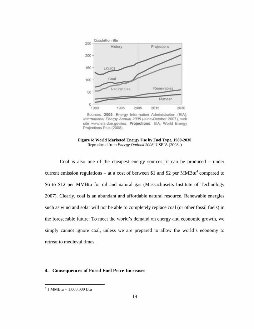
Not only does coal already account for a large percentage of worldwide energy
consumption, the rate at which its share increases is also projected to outpace all other
energy sources (see Figure 6 below). The USEIA (2008a) estimates that coal
consumption is projected to increase by 2.0 percent per year from 2005 to 2030 (by 35
quadrillion Btu from 2005 to 2015 and by another 44 quadrillion Btu from 2015 to 2030),
and it will eventually account for 29 percent of total world energy consumption in 2030.
19
Figure 6: World Marketed Energy Use by Fuel Type, 1980-2030 Reproduced from Energy Outlook 2008, USEIA (2008a)
Coal is also one of the cheapest energy sources: it can be produced – under
current emission regulations – at a cost of between $1 and $2 per MMBtu4 compared to
$6 to $12 per MMBtu for oil and natural gas (Massachusetts Institute of Technology
2007). Clearly, coal is an abundant and affordable natural resource. Renewable energies
such as wind and solar will not be able to completely replace coal (or other fossil fuels) in
the foreseeable future. To meet the world’s demand on energy and economic growth, we
simply cannot ignore coal, unless we are prepared to allow the world’s economy to
retreat to medieval times.
4. Consequences of Fossil Fuel Price Increases
4 1 MMBtu = 1,000,000 Btu
20
An important inquiry relevant to my research is: What will happen to coal use if
substantial price increases are imposed on fossil fuels?
To answer this question, first we must determine the demand and supply price
elasticities for different fossil fuels. For my purpose, I will focus my attention on long-
run elasticities, as the time horizon of the problem I investigate spans at least several
decades.
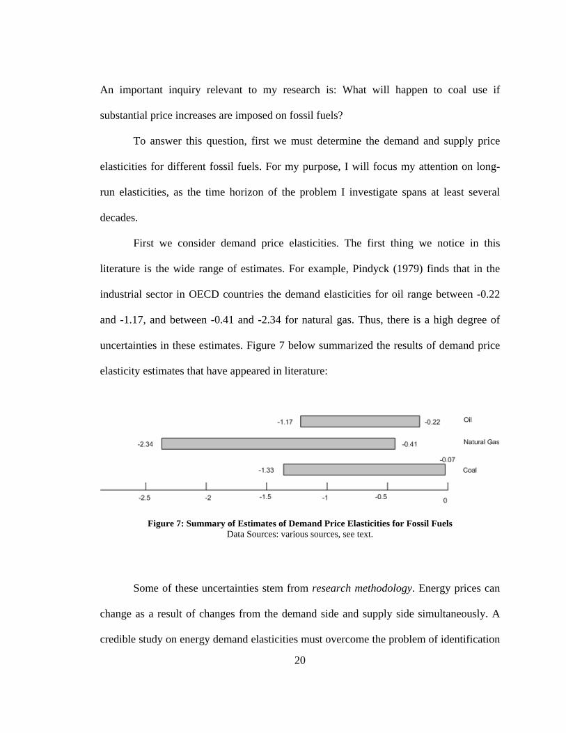
First we consider demand price elasticities. The first thing we notice in this
literature is the wide range of estimates. For example, Pindyck (1979) finds that in the
industrial sector in OECD countries the demand elasticities for oil range between -0.22
and -1.17, and between -0.41 and -2.34 for natural gas. Thus, there is a high degree of
uncertainties in these estimates. Figure 7 below summarized the results of demand price
elasticity estimates that have appeared in literature:
Figure 7: Summary of Estimates of Demand Price Elasticities for Fossil Fuels Data Sources: various sources, see text.
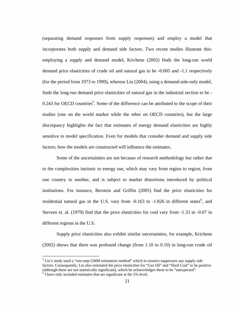
Some of these uncertainties stem from research methodology. Energy prices can
change as a result of changes from the demand side and supply side simultaneously. A
credible study on energy demand elasticities must overcome the problem of identification
21
(separating demand responses from supply responses) and employ a model that
incorporates both supply and demand side factors. Two recent studies illustrate this:
employing a supply and demand model, Krichene (2002) finds the long-run world
demand price elasticities of crude oil and natural gas to be -0.005 and -1.1 respectively
(for the period from 1973 to 1999), whereas Liu (2004), using a demand-side-only model,
finds the long-run demand price elasticities of natural gas in the industrial section to be -
0.243 for OECD countries5. Some of the difference can be attributed to the scope of their
studies (one on the world market while the other on OECD countries), but the large
discrepancy highlights the fact that estimates of energy demand elasticities are highly
sensitive to model specification. Even for models that consider demand and supply side
factors, how the models are constructed will influence the estimates.
Some of the uncertainties are not because of research methodology but rather due
to the complexities intrinsic to energy use, which may vary from region to region, from
one country to another, and is subject to market distortions introduced by political
institutions. For instance, Berstein and Griffin (2005) find the price elasticities for
residential natural gas in the U.S. vary from -0.163 to -1.826 in different states6, and
Stevens et. al. (1979) find that the price elasticities for coal vary from -1.33 to -0.07 in
different regions in the U.S.
Supply price elasticities also exhibit similar uncertainties, for example, Krichene
(2002) shows that there was profound change (from 1.10 to 0.10) in long-run crude oil
5 Liu’s study used a “one-step GMM estimation method” which in essence suppresses any supply side factors. Consequently, Liu also estimated the price elasticities for “Gas Oil” and “Hard Coal” to be positive (although these are not statistically significant), which he acknowledges these to be “unexpected”. 6 I have only included estimates that are significant at the 5% level.
22
supply price elasticity after the establishment of the OPEC quotas. Furthermore, when
considering the impact of price hikes imposed on fossil fuels, we must consider the
substitution effects (cross-price elasticities) between different fossil fuels, and between
fossil fuels and other energies. Estimates of these cross-price elasticities also exhibit a
high degree of uncertainty (e.g. see Reddy 1985). We must also consider the impact of
the increase in fossil fuel prices on economic growth – if the price hike is very large,
since fossil fuels account for such a large portion of global energy use, overall demand
will decrease. Finally, with large price increases, we cannot treat demand or supply
elasticities as uniform along the entire demand and supply curves, but must consider their
values at different points. In short, to fully understand the impact of a substantial price
increase in fossil fuels, we must construct a general equilibrium model that incorporates
all these elements.
Fortunately, a research by Rout et. al. (2008) uses just such a general equilibrium
model. In their research, Rout et. al. use a linear programming (and iterative) computer
simulation model that takes into consideration such factors as extraction of fuels, demand
price elasticities in different sectors, inter-regional trading, etc. to study a 60-70% price
hike on fossil fuels. Although we should not regard this study as anything like a “final
say” in this research, their results give us a glimpse into the impact of a substantial fossil
price hike.
In their research, Rout et. al. consider several different scenarios: price hikes on
one, two or all three fossil fuels (crude oil, natural gas, coal), and with or without a 550
ppmv CO2 stabilization policy. Of interest to us is scenario R1, the reference scenario (no
23
price hikes on any fossil fuels, and no CO2 stabilization), R3 (price hikes on all fossil
fuels, no CO2 stabilization) and S3 (price hikes on all fossil fuels, with CO2 stabilization).
These results are reproduced in Figure 8 below:
Figure 8: Global primary energy supply
(Reproduced from Rout, et. al. (2008))
From the results from Rout. et. al., we can see that in either scenario R3 or S3, in
2030, consumption of coal in absolute quantity will increase relative to the reference
scenario R1 in 2010. These results thus answer our question: even with substantial price
increases on fossil fuels, the portion of global energy supply that comes from coal will
24
remain significant (in the 20-25% range). This reconfirms the relevance and necessity of
my inquiry on the political economy of Clean Coal.
5. Summary
Coal is the most abundant and cheapest fossil fuel. It already contributes a large share to
meet the world’s energy demand. In the U.S., the vast majority of coal (more than 90%)
is used for electricity generation and it accounts for nearly half of the electricity
generation. In the timeframe relevant to my inquiry on the political economy of Clean
Coal – the coming decades or century – coal will remain plentiful and continue to play an
important role in our economic lives. Even in the face of substantial price hikes (60-70%)
on fossil fuels, coal will continue to account for a major portion (about 20-25%) of global
energy use.
25
Chapter 3: Dirtiest fuels of all – externalities of burning coal Coal is the dirtiest of the fossil fuels.
– Phil Barnhart , Oregon State Representative7 1. Introduction
Extracting and burning coal both generate externalities – effects, harmful or otherwise,
that are not borne by the people who extract or burn the coal. The recaptured gaseous,
liquid or solid wastes from burning coal may also generate externalities if not handled
properly.
As of 2007, surface mines produce nearly 70% of U.S. coal (USEIA 2009a).
Indeed the trend is that the percentage of coal from surface mines has been increasing for
the last half century and is continuing to do so (ibid). Surface mining removes large areas
of topsoil or entire mountaintops. This disrupts the hydrology (Bonta, et. al. 1997) and
degrades the soil quality in surrounding regions (Mummey et. al. 2002), and it also
impairs the landscape and causes displeasure to viewers. These are examples of
externalities. However, for the purpose of my dissertation, I shall not focus on
externalities from mining for the reasons stated below.
7 Source: The Creswell Chronicle, “Energy efficiency is key component of state’s economic recovery” by Helen Hollyer, January 21, 2009, website: http://www.thecreswellchronicle.com/news/story.cfm?story_no=6197
26
First, the choice of mining method is determined by the geology and topography
of the coal seam (TEEIC undated8) as well as the economics of extraction. In the United
States, in areas such as the Powder River Basin in Wyoming, there is a vast amount of
coal seam close to the surface that is both physically accessible and economically
recoverable. In addition, the total cost per ton of material handled is normally much lower
in a surface mine than in an underground mine (Nicholas 1992). These factors indicate
that surface mineable coal is not only the most physically accessible; it is also the most
economically recoverable. Because of these factors, as long as surface mineable coal is
abundant, it will be a favored method of production. Indeed, in 2007, the Powder River
Basin alone produced about 42% of total U.S. coal (USEIA 2009a).
Secondly, as I demonstrate in Chapter 2, coal will play a significant role in the
energy future of the United States and the world, accounting for about 25% of global
energy supply in the foreseeable future. Combining this fact with the previously point, we
conclude that surface mining of coal is likely to remain a major production method in the
foreseeable future.
Lastly, the Surface Mining Control and Reclamation Act of 1977 (USOSM 2008)9
and its amendment in 1990 mandate various taxes on coal mined with different methods,
with the highest tax imposed on surface mined coal. These regulations, imperfect as they
may be, to a certain extent internalize the externalities from coal mining10.
8 The TEEIC (Tribal Energy and Environmental Information Clearinghouse) is funded by the U.S. Department of the Interior, website: http://teeic.anl.gov. 9 OSM (Office of Surface Mining Reclamation and Enforcement) is a bureau within the United States Department of the Interior, website: http://www.osmre.gov. 10 I do not imply that these regulations are perfect solutions for an externality problem. In fact, inquiry into them can be a public choice research project in itself. The keyword here is “to a certain extent”.
27
Emissions from burning coal are a different story. As I shall discuss in the next chapter,
modern abatement technologies exist to reduce or eliminate these emissions, so it would
be interesting to investigate whether it is technologically feasible and economically
efficient to employ these abatement methods. For these reasons I shall focus on
externalities from burning coal in my research.
Presently in the United States, about 94% of coal used is for electricity generation
(USEPA, 2008, p. ES-9). Therefore, when we discuss coal use, our primary focus is coal-
fired power plants. It is this use of coal that I focus on in this chapter and throughout this
dissertation.
I also highlight one more fact. The end products (that is, in addition to energy)
from burning coal are gaseous and particulate emissions and solid and liquid wastes. I
discuss the gaseous and particulate emissions in great detail in this chapter, but I shall
point out that the solid and liquid wastes, which in essence are captured pollutants, also
generate externalities if they are not stored properly. The infamous December 2008
Kingston Fossil Plant sludge spill 11 is one example. The TVA (Tennessee Valley
Authority)’s own estimates of the clean-up costs range from $525 million to $824 million
(TVA 2009), which is comparable to the damages from some of the coal generated
pollutants per year in the United States (see next section). Clearly, the proper handling
and storage of wastes are an integral part of internalizing coal generated externalities, a
When coal is burnt, the organic and inorganic materials in it bind with oxygen to generate
heat. But heat is not the only end product of this process. When the materials in coal bind
with oxygen, they form other compounds. The main ingredient of coal – carbon – binds
with oxygen to form carbon monoxide (CO) and carbon dioxide (CO2). Other elements,
such as hydrogen, sulfur and nitrogen also bind with oxygen to form water (H2O), sulfur
dioxide (SO2) and nitrogen oxides (NOx), a mixture of nitrogen-oxygen based compounds.
These gases also lead to the formation of secondary compounds, such as ozone (O3). The
emitted materials are not limited to gases but also include particulate matter (PM).
Particulate matter refers to a mixture of solid particles and liquid droplets found in the air,
it can be further distinguished in two categories: “Inhalable coarse particles” or particles
larger than 2.5 micrometers and smaller than 10 micrometers in diameter (PM10), and
“Fine particles” or particles of 2.5 micrometers in diameter and smaller (PM2.5) (USEPA
2009a). These particles contain harmful material themselves, such as heavy metal
elements and arsenic; they can also become carriers for other substances. Left untreated,
these materials will cause health and environmental hazards.
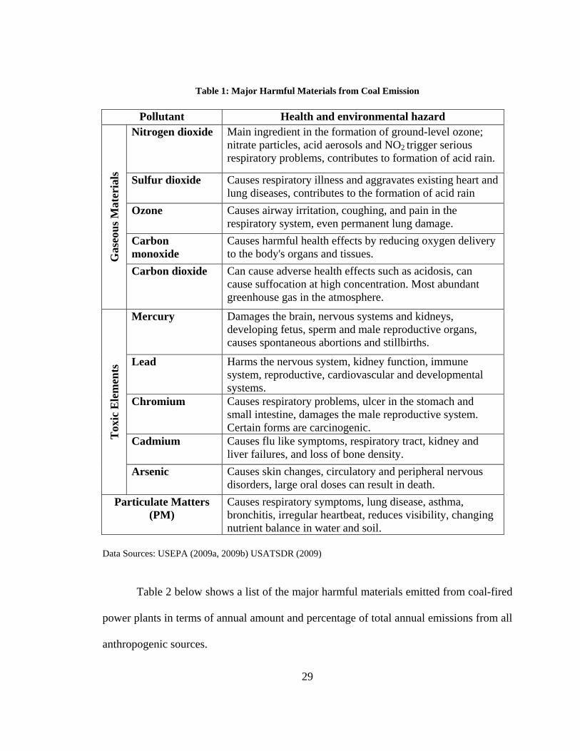
Table 1 lists the major harmful substances emitted from coal-fired power plants:
29
Table 1: Major Harmful Materials from Coal Emission
Pollutant Health and environmental hazard Nitrogen dioxide Main ingredient in the formation of ground-level ozone;
nitrate particles, acid aerosols and NO2 trigger serious respiratory problems, contributes to formation of acid rain.
Sulfur dioxide Causes respiratory illness and aggravates existing heart and lung diseases, contributes to the formation of acid rain
Ozone Causes airway irritation, coughing, and pain in the respiratory system, even permanent lung damage.
Carbon monoxide
Causes harmful health effects by reducing oxygen delivery to the body's organs and tissues. G
aseo
us M
ater
ials
Carbon dioxide Can cause adverse health effects such as acidosis, can cause suffocation at high concentration. Most abundant greenhouse gas in the atmosphere.
Mercury Damages the brain, nervous systems and kidneys, developing fetus, sperm and male reproductive organs, causes spontaneous abortions and stillbirths.
Lead Harms the nervous system, kidney function, immune system, reproductive, cardiovascular and developmental systems.
Chromium Causes respiratory problems, ulcer in the stomach and small intestine, damages the male reproductive system. Certain forms are carcinogenic.
Cadmium Causes flu like symptoms, respiratory tract, kidney and liver failures, and loss of bone density.
Tox
ic E
lem
ents
Arsenic Causes skin changes, circulatory and peripheral nervous disorders, large oral doses can result in death.
Particulate Matters (PM)
Causes respiratory symptoms, lung disease, asthma, bronchitis, irregular heartbeat, reduces visibility, changing nutrient balance in water and soil.
Data Sources: USEPA (2009a, 2009b) USATSDR (2009)
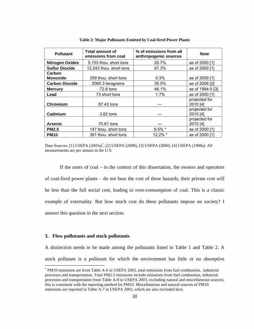
Table 2 below shows a list of the major harmful materials emitted from coal-fired
power plants in terms of annual amount and percentage of total annual emissions from all
anthropogenic sources.
30
Table 2: Major Pollutants Emitted by Coal-fired Power Plants
Pollutant Total amount of emissions from coal
% of emissions from all anthropogenic sources Note
Nitrogen Oxides 5,153 thou. short tons 20.7% as of 2000 [1] Sulfur Dioxide 12,243 thou. short tons 67.3% as of 2000 [1] Carbon Monoxide 359 thou. short tons 0.3% as of 2000 [1] Carbon Dioxide 2065.3 teragrams 35.5% as of 2006 [2] Mercury 72.8 tons 46.1% as of 1994-5 [3] Lead 73 short tons 1.7% as of 2000 [1]
Chromium 87.43 tons --- projected for 2010 [4]
Cadmium 3.82 tons --- projected for 2010 [4]
Arsenic 70.61 tons --- projected for 2010 [4]
PM2.5 147 thou. short tons 6.5% * as of 2000 [1] PM10 361 thou. short tons 12.2% * as of 2000 [1]
Data Sources: [1] USEPA (2003a)*, [2] USEPA (2008), [3] USEPA (2000), [4] USEPA (1998a). All measurements are per annum in the U.S.
If the users of coal – in the context of this dissertation, the owners and operators
of coal-fired power plants – do not bear the cost of these hazards, their private cost will
be less than the full social cost, leading to over-consumption of coal. This is a classic
example of externality. But how much cost do these pollutants impose on society? I
answer this question in the next section.
3. Flow pollutants and stock pollutants
A distinction needs to be made among the pollutants listed in Table 1 and Table 2. A
stock pollutant is a pollutant for which the environment has little or no absorptive * PM10 emissions are from Table A-6 in USEPA 2003, total emissions from fuel combustion, industrial processes and transportation. Total PM2.5 emissions include emissions from fuel combustion, industrial processes and transportation from Table A-8 in USEPA 2003, excluding natural and miscellaneous sources; this is consistent with the reporting method for PM10. Miscellaneous and natural sources of PM10 emissions are reported in Table A-7 in USEPA 2003, which are also excluded here.
31
capacity (Maatta 2006) – in other words, a pollutant that stays in the environment for a
long time. A flow pollutant, in contrast, does not accumulate in the environment. Some
pollutants are strictly flow pollutants, such as light and noise, for there can be no
“accumulation” of them. For pollutants with a very short environmental half-life (or
environmental half-time – the time necessary for one-half of the pollutant to be removed
from the environment), we can approximate them as flow pollutants. Other pollutants
have a very long environmental half-life and should be treated as stock pollutants. When
considering the externality stock pollutants cause, we must consider the effects of the
flow within a given period and the effect of the current stock.
Among the pollutants listed in Table 1 and Table 2, some have relatively short
environmental half-life. The environmental half-life of SO2 is on the order of 3 days
(Hocking 2006). NOx, a mixture of nitrogen-oxygen compounds, is rapidly oxidized into
nitrogen dioxide (NO2), which has a half-life of about 50 days (ibid). PM also has a short
environmental half-life on the order of hours (Kruizea, et. al. 2003).
Other pollutants, such as heavy metals and arsenic, are toxic elements. Strictly
speaking, the only way for them to diminish in the environment is through radioactive
decay. For the most stable isotopes of these elements, the radioactive decay half-life can
be extremely long (20Hg, an isotope of mercury, and 75As, an isotope of Arsenic, are both
radioactively stable12 – that is, they do not exhibit any radioactive decay). For these toxic
elements, what is important is how long they will remain in the food chain and drinking
water. These can also be a very long times – for example, the environmental half-life for
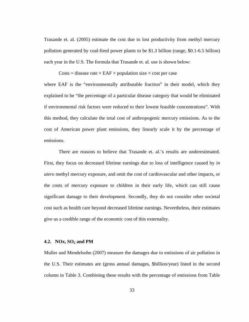
Muller and Mendelsohn’s analysis focuses on air pollution only. They consider
seven categories of damages: mortality, morbidity, agriculture, timber, visibility,
materials and recreation. From the text and the references they use, it is evident that they
also consider the effects of acid rain. For gaseous pollutants, such as NOx and SO2, they
are likely to capture the full effects of damages. For particulate matter, since Muller and
Mendelsohn do not specifically consider the composition (what toxic elements it contains)
and the fact that PM can become carriers of other pollutants, it is possible that they may
have underestimated its effect. This is supplemented by my estimates of toxic elements in
the next section.
4.3. Arsenic, Chromium and Cadmium
35
The first-hand estimates of arsenic, chromium and cadmium pollutions in the United
States are unavailable to the best of my knowledge. However, in a study on air pollution
cost estimates for Europe, Spadaro and Rabl (2002) give estimates for arsenic, cadmium
and chromium (among other pollutants) in terms of costs per kilogram of pollutants (ibid,
p90, Table 6). As we can see in Table 2, the amount of cadmium from coal is quite small
compared with other pollutants, nonetheless, since Spadaro and Rabl’s results already
include cadmium, I shall also include it in my estimates.
My estimation method is to apply Spadaro and Rabl’s per-kilogram estimates to
the U.S. with appropriate conversions. The conversions I make in this computation are as
follows: First, Spadaro and Rabl’s studies are based on a population density of 80
persons/km2. The United States’ population density as of 2000 is 28.6 persons/ km2. (U.S.
Census Bureau 2009, USCIA 2009)13. Thus, I multiply their results with a “population
scaling factor”, which we designate as p. The value of p is shown below:
p = 28.6 / 80 = 0.36
Second, we also need to consider currency conversion as the estimates in this
study are denominated in euros. We note that Spadaro and Rabl’s paper was published in
the first issue of International Journal of Risk Assessment and Management in 2002,
therefore, I use the exchange rate as of end of 2001. This exchange rate is 0.8913 euro for
a dollar14, which we designate as e:
13 According to U.S. Census Bureau (2009), the total population in 2000 is 281,421,906; according U.S. CIA, the total area of the United States is 9,826,675 km2. Dividing the former number by the latter, we obtain a population density of 28.6 persons/ km2. 14 According to http://finance.yahoo.com/currency-investing, cross-checked with multiple sources.
36
e = 0.8913
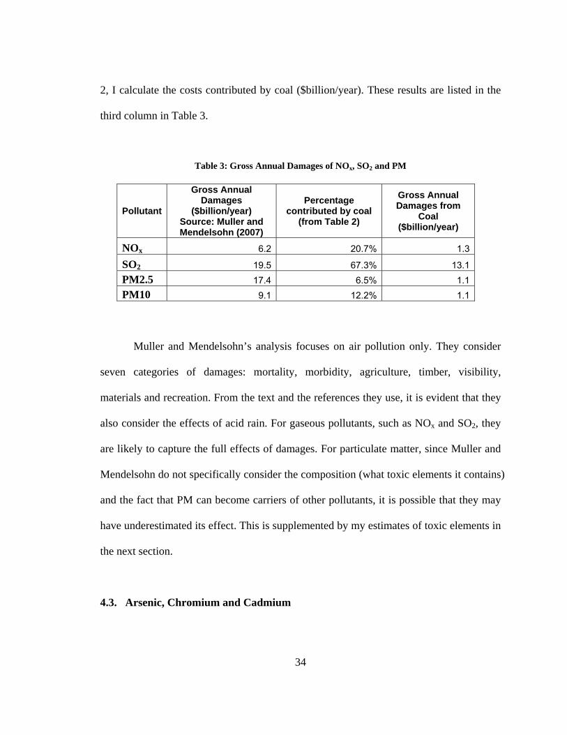
Then I use the total emission amounts (which I designate as w, which I also
convert to kilograms) in Table 2 and the costs per kilogram (which we designate as c)
from Spadaro and Rabl (2002) to compute the total externality costs caused by these
pollutants. Thus, the formula I use is:
Total cost of pollutant = c × w × p × e
The results are summarized in Table 4 below:
Table 4: Total costs of Arsenic, Chromium and Cadmium
The estimated costs caused by each pollutant in Table 5 represent the costs per year,
which is to say, they are the estimated annual costs of the flow pollutants. As discussed in
the previous section, for toxic elements, there are also stocks of them in the environment,
which will continue to cause harm and impose a cost to society. When analyzing the
externality costs, we must take both stock and flow externalities into account, although
there may be little we can do about the stock of accumulative negative externalities.
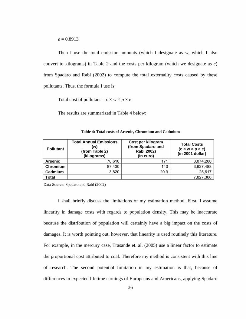
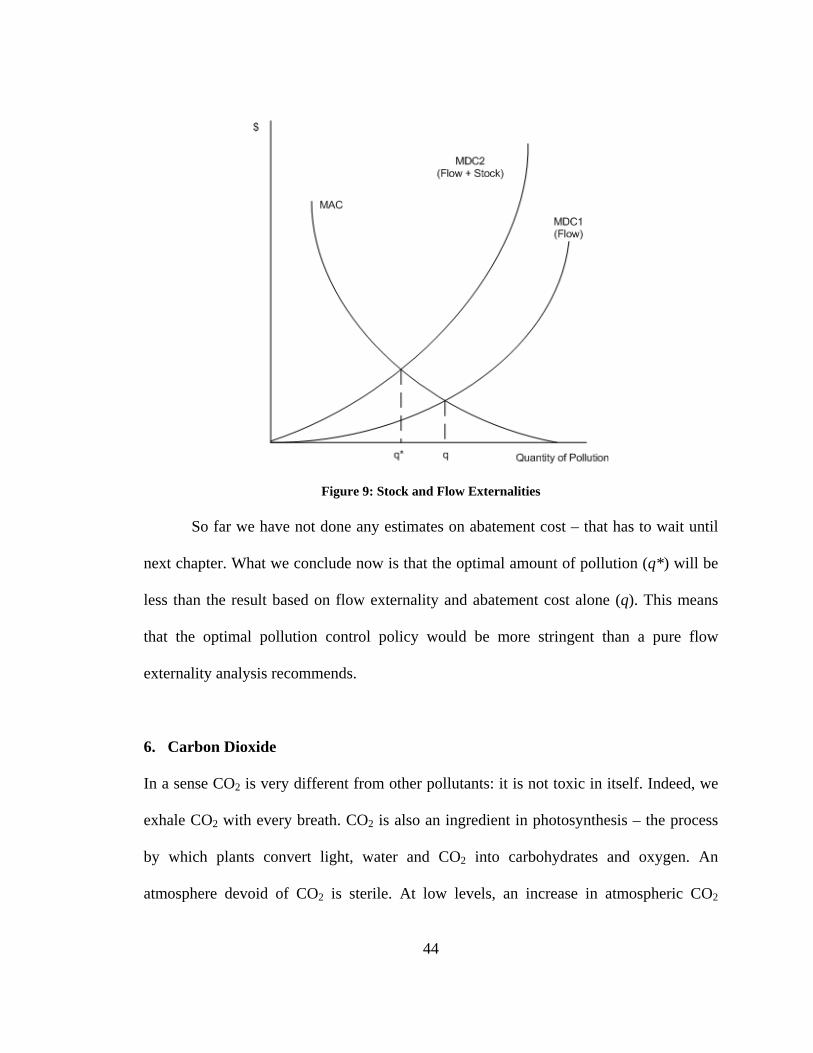
The diagram in Figure 9 below illustrates this point. The marginal abatement cost
(MAC) curve represents the marginal abatement cost. It is downward sloping because as
43
pollutants are being removed from the environment, it becomes more costly to remove
each additional unit. The first marginal damage cots curve (MDC1) represents the
marginal damage cost caused by flow pollutants. If we only analyze flow pollutants, we
will come to the (incorrect) conclusion that the optimal amount of pollution is at the
intersection of the MAC and MDC1 curve, q. However, because there are stock
pollutants in the environment, we must take the effects of both stock and flow pollutants
into consideration. The second marginal damage cost curve (MDC2) represents the
marginal damage cost of the externality caused by both the stock and flow pollutants.
Because MDC2 represents the sum total of the marginal costs of stock and flow
pollutants, it always lies above the MDC1 curve. The optimal amount of pollution, then,
is at the intersection of the MAC and MDC2 curve, q*, which always lies to the left of
(i.e. less than) q.
44
Figure 9: Stock and Flow Externalities
So far we have not done any estimates on abatement cost – that has to wait until
next chapter. What we conclude now is that the optimal amount of pollution (q*) will be
less than the result based on flow externality and abatement cost alone (q). This means
that the optimal pollution control policy would be more stringent than a pure flow
externality analysis recommends.
6. Carbon Dioxide
In a sense CO2 is very different from other pollutants: it is not toxic in itself. Indeed, we
exhale CO2 with every breath. CO2 is also an ingredient in photosynthesis – the process
by which plants convert light, water and CO2 into carbohydrates and oxygen. An
atmosphere devoid of CO2 is sterile. At low levels, an increase in atmospheric CO2
45
concentration stimulates plant growth and is therefore beneficial (Amthor 1995). Only at
above 10,000 ppm – a level significantly higher than the current atmospheric CO2
concentration (~ 380 ppm) – does it start to pose some health risks (Rice 2003).
Therefore, when we discuss the harmful effects of CO2, we are not concerned with the
direct health hazard it causes, but with its potential to cause global warming (see Chapter
1).
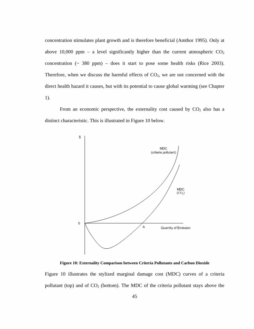
From an economic perspective, the externality cost caused by CO2 also has a
distinct characteristic. This is illustrated in Figure 10 below.
Figure 10: Externality Comparison between Criteria Pollutants and Carbon Dioxide
Figure 10 illustrates the stylized marginal damage cost (MDC) curves of a criteria
pollutant (top) and of CO2 (bottom). The MDC of the criteria pollutant stays above the
46
horizontal axis across the entire range of quantity of emission, which is to say, it causes
harm at any quantity. The MDC curve of CO2 is quite different: initially it dips below the
horizontal axis, which means that at low levels it in fact generates a benefit. Only at some
given quantity of emission (point A) does CO2 cause a positive damage cost.
Regarding the cost of CO2, different sources give widely varied estimates. The
much-publicized and much-criticized “Stern Review” (Stern 2006) estimates that “if we
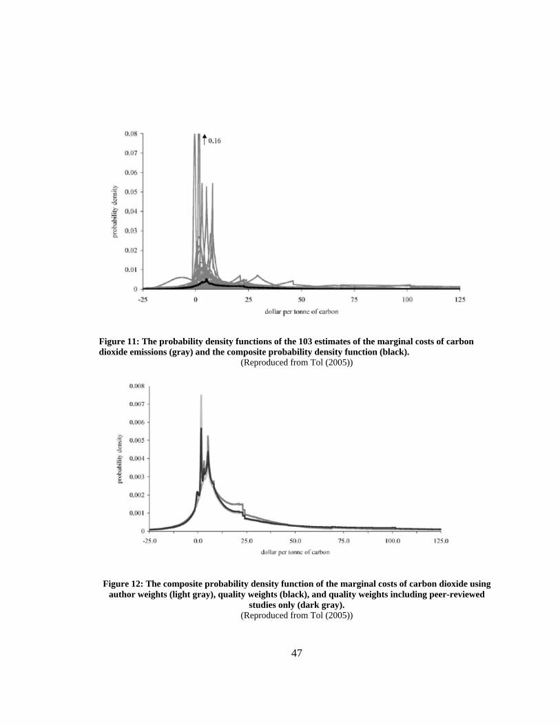
don’t act … the overall costs and risks of climate change will be equivalent to losing at
least 5% of global GDP each year, now and forever”, and “if a wider range of risks and
impacts is taken into account”, the cost could “rise to 20% of (global) GDP or more (now
and forever)”. This would be an enormous cost to society of apocalyptic proportions.
Other studies generally produce more moderate and realistic results. Tol (2005) conducts
survey of 28 published studies that contain 103 estimates. He uses four different ways to
combine these results to plot the probability density function of the cost damage
estimates:
1. “simple average” which gives equal weight to each estimate (not each study, as
some studies contain more than one estimate)
2. “author weights” which gives equal weight to each study
3. “quality weights” which considers five criteria including whether the study is
peer-reviewed, whether it estimates the marginal damage costs rather than
average costs and the age of the study
4. “peer-reviewed only” which only includes peer-reviewed articles.
These results are reproduced in Figure 11 and Figure 12 below.
47
Figure 11: The probability density functions of the 103 estimates of the marginal costs of carbon dioxide emissions (gray) and the composite probability density function (black).
(Reproduced from Tol (2005))
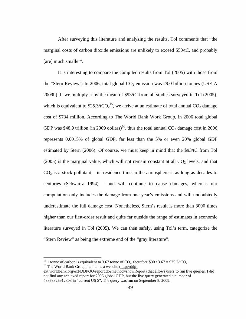
Figure 12: The composite probability density function of the marginal costs of carbon dioxide using author weights (light gray), quality weights (black), and quality weights including peer-reviewed
studies only (dark gray). (Reproduced from Tol (2005))
48
For all studies (Figure 11), the CO2 damage cost estimates have a mean of $93/tC
(tonne of carbon), a median of $14/tC and a mode of only $1.5/tC; for peer-reviewed
studies only (Figure 12), the mean is $50/tC, the median is $14/tC and the mode is $5/tC
(for brevity, I shall skip the “author weights” and “quality weights” results).
From the results compiled by Tol, we draw the following conclusions:
1. There is an enormous degree of uncertainty in CO2 damage cost estimates. The
range of estimates is very large: one study even has an estimate of $1666.7/tC, or
about 118 times larger than the median. The standard deviations are also very
large: it is $203/tC for all results, or about 2.2 times the arithmetic mean.
Considering that the estimates are strongly right-skewed (most estimates are in
the lower part of the range), the uncertainty is even more pronounced, as can be
seen in Figure 11.
2. Interestingly, but not surprisingly, some estimates are negative (benefits), as can
be seen in Figure 11 and Figure 12. This means the uncertainty is not merely
about the magnitude of CO2 damage cost, but also its nature (whether it is “good”
or “bad”).
3. Another interesting thing is that peer-reviewed studies have a lower mean and
smaller standard deviation. This is evidenced by comparing Figure 11 and Figure
12. This leads the author to observe that “a substantial part of the larger cost
estimates are in the so-called gray literature” and remark that “[i]t seems as if the
most pessimistic estimates of climate change impacts do not withstand a quality
test”.
49
After surveying this literature and analyzing the results, Tol comments that “the
marginal costs of carbon dioxide emissions are unlikely to exceed $50/tC, and probably
[are] much smaller”.
It is interesting to compare the compiled results from Tol (2005) with those from
the “Stern Review”: In 2006, total global CO2 emission was 29.0 billion tonnes (USEIA
2009b). If we multiply it by the mean of $93/tC from all studies surveyed in Tol (2005),
which is equivalent to $25.3/tCO215, we arrive at an estimate of total annual CO2 damage
cost of $734 million. According to The World Bank Work Group, in 2006 total global
GDP was $48.9 trillion (in 2009 dollars)16, thus the total annual CO2 damage cost in 2006
represents 0.0015% of global GDP, far less than the 5% or even 20% global GDP
estimated by Stern (2006). Of course, we must keep in mind that the $93/tC from Tol
(2005) is the marginal value, which will not remain constant at all CO2 levels, and that
CO2 is a stock pollutant – its residence time in the atmosphere is as long as decades to
centuries (Schwartz 1994) – and will continue to cause damages, whereas our
computation only includes the damage from one year’s emissions and will undoubtedly
underestimate the full damage cost. Nonetheless, Stern’s result is more than 3000 times
higher than our first-order result and quite far outside the range of estimates in economic
literature surveyed in Tol (2005). We can then safely, using Tol’s term, categorize the
“Stern Review” as being the extreme end of the “gray literature”.
15 1 tonne of carbon is equivalent to 3.67 tonne of CO2, therefore $90 / 3.67 = $25.3/tCO2. 16 The World Bank Group maintains a website (http://ddp-ext.worldbank.org/ext/DDPQQ/report.do?method=showReport) that allows users to run live queries. I did not find any achieved report for 2006 global GDP, but the live query generated a number of 48863326912303 in “current US $”. The query was run on September 8, 2009.
50
7. Two Types of Uncertainties
We have seen in this chapter that there are many sources of uncertainties with regards to
the effects of coal-generated externalities. But we must distinguish between two very
different types of uncertainties.
The first type is the uncertainty in estimating the magnitude and cost of a
pollutant. This type of uncertainty stems from the complex and dynamic nature of
environmental and economic issues, accuracies and completeness of reporting,
measurement methodologies and so on. For this type of uncertainty, in theory at least, as
we continue to deepen our understanding of the underlying scientific and economic issues
and perfect our measurement and reporting techniques, we will be able to obtain more
and more accurate results. I call this type of uncertainty “technical uncertainty”.
The second type of uncertainty is the uncertainty in our understanding of the
effects of a pollutant. If our understanding of the role that a substance plays in affecting
the natural environment and human health is unclear or immature, then even if we have
the best techniques to measure the quantity of this material and trace its flow throughout
the environment, our estimate of its economic effect will not be fundamentally sound. I
call this type of uncertainty “theoretical uncertainty”, which is similar to the “model
uncertainty” in economic literature (Rowley and Smith 2009, p.70), that is, we do not
know or are not sure what model best describes the real world. If a substance exhibits a
considerable degree of theoretical uncertainty, it is imperative that we have the correct
understanding of its nature before taking costly actions changing its level.
51
Technical uncertainty will always be present as it is impossible to get the
“perfect” measurement of the effects of a pollutant. But the degree of theoretical
uncertainty varies substantially from one pollutant to another. For example, although
ozone in the stratosphere (“ozone layer”) filters out harmful ultraviolet rays from the sun
and is therefore beneficial to human health, ground level ozone, which is a derivative
from nitrogen oxides emitted from coal-fire power plants, causes various health hazards,
as shown in Table 1. Since the net transport of ozone between the stratosphere and the
troposphere (the layer of atmosphere closest to the Earth) is downward (Collins, et. al.
2002)17, ground-level ozone does not contribute to the ozone layer, thus its net effect is
unequivocally harmful. There is even less ambiguity regarding the harmful health and
environmental effects of other pollutants, such as nitrogen oxides, sulfur dioxide, arsenic
and heavy metals. Therefore, the theoretical uncertainty of these criteria pollutants is
virtually eliminated.
The situation is quite different in the case of CO2. As I discussed in Chapter 1,
there are still ongoing debates about the effects of global warming, and the role CO2
plays in causing it. Regional effects, the difficulty in capturing human adaptation in
impact analysis further complicate the issue (Tol 2005). Additionally, models are often
highly sensitive to the choice of time preference and require assumptions about the
relative importance of impacts in different sectors and regions, which all involve
(subjective) value judgments (ibid). Consequently, the uncertainty about CO2’s effects to
human societies is of the “theoretical” type. Furthermore, as I illustrated in Figure 10,
17 Although this is beyond my area of studies, intuitively, ozone (O3) is a much heavier gas than atmosphere, which probably partially explains the predominantly downward movement.
52
CO2 is actually beneficial at low levels, a characteristic distinct from other pollutants, and
indeed as we can see in Figure 11 and Figure 12, some studies estimate that there is a net
benefit in increased atmospheric CO2 concentration levels. If we cannot pinpoint the level
at which the marginal benefit of CO2 turns into a marginal cost (point A in Figure 10),
then we may mistake a benefit for cost. Therefore, greater caution needs to be taken when
dealing with externalities with theoretical uncertainty. It may require a different strategy
dealing with them than what is used to deal with externalities without theoretical
uncertainty, a point that I shall return to later in this dissertation.
8. Corrections for Coal-generated Externalities
As discussed in this chapter, burning coal generates externalities, most of which are
harmful. If there are some institutional constraints – whether tax, subsidy, direct
regulation, or a combination of these – imposed upon the owners of coal-fired power
plants to internalize these externalities, what are the measures they can employ to correct
these externalities?
The most primitive measure is dilution – to disperse pollutants into the
environment. There is an old saying “the solution to pollution is dilution”. Primitive as it
is, dilution actually has its scientific and economic grounding. Dilution has the following
effects:
1. The ecosystem has a certain level of assimilative capacity (Perman, et. al., 2003,
pp.168-9). At low concentration, the ecosystem is able to assimilate pollutants.
When there are few power plants and they are dispersed geographically, dilution
53
is an effective solution to mitigating or even elimination pollution. However,
when the concentration of pollutants exceeds the assimilative capacity of the
ecosystem, dilution is not an appropriate approach.
2. Detection instruments have sensitivity thresholds. Dilution makes the pollutants
harder to detect. In the case where multiple pollution sources are involved, the
instruments may be able to detect the total level of pollution, but it may be harder
to trace back to each source.
For the owners of coal-fired power plants, dilution is almost certainly less costly
than abatement (which involves capturing and safely storing the pollutants). For the
victims, dilution has the following effects:
1. It lowers the harmful effects to each victim.
2. It converts a private externality to a public externality (Baumol and Oates, 1988),
or at least a "more private" externality to a "more public" one, and disperses the
pollutants to a wider area so that the number of victims will increase.
3. By including more victims, it raises the transaction cost for collective action for
the victims.
Thus, there is a powerful incentive for the polluters to use dilution rather than
abatement as a pollution control measure. The most common way to dilute is to build
taller smokestacks to disperse the emissions above the inversion layer (a layer in the
atmosphere in which the usual temperature gradient – warm air below cold air – is
reversed such that pollutants below it are trapped locally) (Jensen and Bourgeron 2001).
54
There is evidence that taller smokestacks can improve local air quality without reducing
total emissions (Bellas and Lange, 2008).
Unfortunately, as the number of polluters increase, dilution will lose its
effectiveness because the amount of pollution will eventually exceed the assimilative
capacity of the environment. Further, even though the pollution from each polluter gets
diluted, the total amount of pollution will still add up in the environment. The sum total
of disutilities faced by the victims (measured by willingness to avoid) and the cost of
dilution may exceed the total cost of abatement, resulting in a suboptimal outcome. I
believe this “many polluters, many victims, dispersed pollution” scenario accurately
depicts reality, evidences include:
1. There are many sources of emissions. There are 616 coal-fired power plants in the
U.S. alone (USEIA 2008) and one is built in every week to 10 days in China18.
2. The pollutants are dispersed widely. Satellite images have shown that plume from
Chinese core-fired power plants can propagate over the Pacific Ocean and reach
the west coast of the United States (USNASA 2008).
This “many polluters, many victims” situation significantly raises the transaction
cost between polluters and victims, which makes Coasian bargain (Coase 1960) to reach
Pareto efficient outcome unrealistic. Furthermore, when the effects of some of the
pollutants, such as acid rain from SO2 and global warming from CO2 (insofar as we
believe that is one of the major causes for global warming) are global in scale, the
18 New York Times, June 11, 2006, Pollution From Chinese Coal Casts a Global Shadow, By Keith Bradsher and David Barboza
55
victims’ choices, such as “moving away from the nuisance”, is also no longer be feasible.
Under these conditions, as Baumol and Oates (1988, Chapter 3) illustrate, the proper
device is a Pigouvian tax equal to marginal social damage levied on the generator of the
externality with no supplementary incentive for victims. The case for coal is a bit more
complicated than the textbook example because taxes and regulations are already
imposed on coal and coal-fired power plants, and in the U.S. there is a SO2 permit-trading
program in effect. In addition, in this chapter I only look at the damage cost side of the
problem. To determine whether it is efficient to use modern abatement technologies for
coal-fired power plants, we must look at the abatement cost side of the issue, which I
shall discuss in the next chapter. The discussion here points out that in the world we
inhabit today, dilution alone is an inadequate measure to control pollution and will lead to
economically inefficient outcomes. Modern abatement technologies, and policy
instruments that provide proper incentive for polluters to adopt these technologies, should
be considered as meaningful pollution control measures. These will be the focus of
following chapters.
9. Summary and Conclusion
Coal, more specifically coal-fired power plants generate a range of pollutants that cause
health and environmental hazards. These health and environmental hazards become
externalities when the operators of coal-fired power plants do not have to bear their full
cost. In this chapter I give damage cost estimates to all major coal-generated criteria
pollutants by critically reviewing and synthesizing this literature, and performing my own
56
estimates. I also discuss the difference between stock and flow pollutants. The case of
CO2 is very different than other pollutants as it is beneficial at lower levels. I critically
review a survey of the damage cost estimates of CO2. In doing so, I also make a
distinction between two types of uncertainties – technical uncertainty and theoretical
uncertainty. I conclude that technical uncertainty exists for all pollutants, but for CO2, a
high degree of theoretical uncertainty also exits. This requires greater caution when
dealing with the abatement of CO2. Finally, I discuss why the primitive method of
dilution is no longer effective in a world with “many polluters, many victims”, and
conclude that the combination of a Pigouvian tax and modern abatement technologies
(which I shall discuss in the next chapter) provide the most appropriate corrective
measure.
57
Chapter 4: Clean Coal Technologies Clean coal is like healthy cigarettes. It does not exist.
– Al Gore, Former Vice President of the United States19 I believe the future of clean coal is very bright.
– Joe Lucas, Spokesman for American Coalition for Clean Coal Electricity20 1. Introduction: What is Clean Coal?
“Clean Coal” is a confusing term; it means different things to different people, as the
opening quotations suggest. To some people, it means 100% carbon capture and
sequestration (CCS) in coal-fired power plants. This is the stance that many
environmental activists take. At present, no commercial coal-fired power plants utilize
CCS technologies; this is what Al Gore means when he says Clean Coal “does not exist”.
To others, however, “Clean Coal” is just an umbrella term that encompasses
modern abatement technologies – not merely CCS, but including abatement for SO2, NOx,
PM and all kinds of pollutants from coal-fired power plants described in Chapter 3. This
was in fact the most common usage of the term “Clean Coal Technologies” in
19 Taking On King Coal by Bryan Walsh, Time magazine, Nov. 05, 2008, website: http://www.time.com/time/magazine/article/0,9171,1856987-1,00.html 20 McCain, Obama tout coal, But investor skepticism evident in scant interest in Colorado firms by Gargi Chakrabarty, Rocky Mountain News, October 31, 2008, website: http://www.rockymountainnews.com/news/2008/oct/31/mccain-obama-tout-coal
58
engineering communities and publications before CO2 became a hot topic (for example,
see McMullan, et. al. 1997).
In this dissertation I adopt the latter convention used in engineering literature, that
is, I use “Clean Coal” or “Clean Coal Technologies” to refer to modern technologies that
reduce emissions of any pollutant, not just CO2. I do so for two reasons: First, this was
the convention before the current debate about CO2 and CCS. Continuing with this
convention puts my research in the proper historical context. Secondly, as I summarize in
Chapter 3, there are many types of pollutants emitted from coal-fired power plants, there
is no particular reason why the abatement of CO2 should take higher priority than the
abatement of other pollutants. In fact, as I discuss in Chapter 3, there is still a
considerable degree of theoretical uncertainty about the damage cost of CO2 and this
theoretical uncertainty is virtually nonexistent in criteria pollutants. Therefore, abatement
of criteria pollutants should take higher priority. Equating “Clean Coal” with CCS would
imply that the abatement of CO2 is of paramount importance, which does not reconcile
with facts from scientific and economic literature.
But what is a “modern” technology? This modifier suggests a level of subjectivity.
On the spectrum of abatement (and dilution) technologies, there are very primitive ones
and ones that reflect the state-of-the-art engineering achievement of our time. At one end
of this spectrum, we have building taller smokestacks and dispersing the pollutants. I do
not consider this to be a “Clean Coal Technology”. At the other end, we have IGCC
(Integrated Gasification Combined Cycle), a process that converts coal into syngas
(synthesis gas) that consists mainly of carbon monoxide (CO) and hydrogen. This
59
technology has the potential of virtually eliminating all criteria pollutants from coal. I
consider IGCC to be a Clean Coal Technology.
In between them, there are some gray areas. For example, the vast majority – all
except 2 (USEIA 2009a) – of coal-fired power plants built in the last half century use a
technology called pulverized coal (PC) combustion or one of its variants (more on this in
the next section). There are technologies, such as chemical cleaning, scrubbers and
electrostatic precipitators to reduce emissions from PC combustion plants. Indeed, these
technologies have helped to produce a 38% reduction in total SOx emissions, and 25%
reduction in total NOx emissions from coal-fired power plants in the last 30 years (MIT
2007, p23). However, as I demonstrate Chapter 3, even with these technologies, coal-
fired power plants still generate large amounts of pollutants which impose negative
external cost on society. Because of the nature of PC combustion, further emission
reduction becomes prohibitively expensive and economically unviable. For these reasons,
I do not consider PC combustion technologies to be “Clean Coal Technologies”.
IGCC is a totally different mechanism – it gasifies coal to produce syngas, which
is then burned to generate heat. This means most solid material is “left behind” during the
gasification process, making them easier to capture. Also, the generated syngas is kept at
a high pressure which makes the removal of pollutants more technically and
economically effective than cleaning up large volumes of low pressure flue gas (MIT
2007, p 141). Because of these factors, I consider IGCC, with or without CCS, to be a
“Clean Coal Technology”.
60
2. Current Technologies Used in Coal-fired Power Plants in the United States
There are mainly two major types of coal-fired power plants: pulverized coal (PC)
combustion and IGCC. “Pulverization” is a process to grind coal to very fine particles,
which are then injected through the burners into the furnace with combustion air and
burned there. Depending on the pressure and temperature at which the pulverized coal is
burned, PC combustion can be further divided into subcritical (~ 550°C, ~3200 psi),
supercritical (~ 565°C, ~3530 psi) and ultra-supercritical (>565°C, and at pressures in the
4000-6000 psi range). A variation of PC is fluid-bed combustion, in which the pulverized
coal is burned in a “bed” of upward-blowing jets of air, typically a circulating fluid bed
(CFB).
IGCC is essentially a combination of two processes, the second of which also
contains two electricity-generating cycles (hence the words “integrated” and “combined
cycle”). In the first step, coal is gasified to produce syngas. The syngas is further cleaned,
and then burned in a gas turbine to drive a generator. Because the syngas is burned at a
much higher temperature (>1000°C) than PC combustion units, the turbine exhaust is
also at a very high temperature and goes into a heat recovery generator to produce steam
to drive a steam turbine. Because of the two electricity generating cycles, generating
efficiency is very high in IGCC plants – IGCC plants can achieve a generating efficiency
of 38.4%, higher than the current average efficiency of 34% in PC plants, although super-
critical and ultra-supercritical PC plants can also achieve similar efficiencies (Beer 2007).
Higher efficiency means that for a given unit of electricity, less coal is burned; this also
helps reduce emissions.
61
At the end of 2008, there are 601 coal-fired power plants with 1458 generating
units in the United States, 1415 of these units are in operating or standby (backup) status,
with a total capacity of 333241 megawatts. Of these, the vast majority is of the PC design
type; only 3 units at 2 plants (1 unit at the Wabash River Station in Vigo County, Indiana
and 2 units at the Polk Station in Tampa, Florida) are IGCC units. These 3 units represent
a mere 0.2% of the total number of generating units, and their 518 megawatts generating
capacity represents only about 0.16% of the total generating capacity of all operating and
standby power plants (USEIA 2009a). Table 6 below shows the descriptive statistics of
all coal-fired power plants in the U.S.
Table 6: Descriptive Statistics of All Coal-fired Power Plants in the United States
Total number of coal-fired power plants 601 Total number of generating units 1458 Operating and standby units Number of units 1415 Total Capacity (mW) 333241.1 Mean Age 41.1 IGCC units Number of units 3 Total Capacity (mW) 518.3 Mean Age 12.6 Out of service units Number of units 41 Total Capacity (mW) 3031.8 Mean Age 52.4
Data Source: USEIA (2009c)21
21 USEIA 2009a divides these power plants in 5 categories in terms of operating status: operating (OP), standby/backup (SB), out of service, but will be returned to service in the next calendar year (OA) and out of service and not expected to be returned in the next calendar year (OS), and retired (RE). No plants of status RE is listed, and only 2 of status OA are listed. Table 1 includes plants of status OP and SB in the “Operating and standby” category, but only includes plants of status OS in the “Out of service” category.
62
Figure 13 below shows these plants grouped by their initial year of operation in 5-
year intervals (except the first group, which has a 6-year interval of 1924-1930 because
there is only 1 plant with an initial year of operation of 1924; and the last group which
has a 3-year interval because no data is available yet for 2009 and 2010).
All Coal-fired Power Plants Grouped by Initial Year of Operation
122
17 22
73
243
188
146156
123 130112
98
54
18 11 10
0
50
100
150
200
250
300
1924
--193
0
1931
--193
5
1936
--194
0
1941
--194
5
1946
--195
0
1951
--195
5
1956
--196
0
1961
--196
5
1966
--197
0
1971
--197
5
1976
--198
0
1981
--198
5
1986
--199
0
1991
--199
5
1996
--200
0
2001
--200
5
2006
--200
8
Initial Year of Operation
Num
ber o
f Gen
erat
ing
Uni
ts
Figure 13: All Coal-fired Power Plants in the United States Grouped by Initial Year of Operation
Data Source: USEIA (2009c)
The most interesting thing we note in Figure 13 is that, since the typical lifespan
of a coal-fired power plant is 40-50 years (Pouris 1987, Kahrl and Roland-Holst 2006,
Holdren 2007), 557 or 39% of these units are already operating beyond their “life
expectancy”, and in the next 20 years, that number will almost exactly double, to 1112.
What causes these plants to operate beyond their typical “life expectancy”? This is a
63
puzzle that be unraveled later in my dissertation, but for now, the important point we
take from the descriptive statistics is that in the coming couple of decades, a large
percentage of coal-fired power plants will need to be replaced. So the question we want
to ask is: what should we replace them with?
3. The Case for IGCC without Considering CCS
MIT (2007, Chapter 3) gives a list of “levelized COE (cost of electricity)” (meaning fully
accounted for capital, operation, maintenance and fuel costs) for each plant type. These
numbers are reproduced in Table 7 below.
Table 7: Levelized Cost of Electricity for Each Plant Type
Plant Type Cost of Electricity (c/kw-h)
Subcritical PC 4.84Supercritical PC 4.78Ultra-supercritical PC 4.69Subcritical CFB 4.68IGCC 5.13
Data Source: MIT (2007)
From Table 7 we see that power plants of the PC design can produce electricity
more cheaply than IGCC plants. However, these numbers do not include externality costs
– costs caused by pollutants emitted from these plants. To compare their “true costs”, we
must take externality costs into account.
As I show in the previous section, the current fleet of coal-fired power plants in
the U.S. is predominantly of the PC design (including CFB). For simplicity, I shall take
64
the average of the COEs for these plant types from Table 7 to represent that of existing
coal-fired power plants – this number is 4.75 c/kw-h. From MIT (2007), we also obtain
the emission numbers for PC and IGCC plants. Combining these with the externality
costs I obtain in Chapter 3, we can then calculate the FCOE (Full Cost of Electricity,
inclusive of externality costs) for PC and IGCC power plants (see Appendix). These
numbers are listed in Table 8 below:
Table 8: Full Cost of Electricity Comparison of Existing Plants and IGCC Plants
Data Sources: MIT (2007), USEIA (2009b), Chapter 3 of current dissertation
From Table 8, we see that once externality costs are considered, the full cost of
electricity (FCOE) for IGCC plants is actually lower than existing coal-fired power plants.
Actually, the externality costs in Table 8 only includes the damage costs of NOx, SO2,
Mercury and PM, since IGCC plants generate less emissions than PC plants in almost
every category, if other pollutants were included, the cost discrepancy would be even
larger.
In order to avoid over-reliance on one study, I conduct a second comparison (see
Appendix A) based on different sources (Phillips 2005, MPCA 2006 and USEIA 2009b),
these results are listed in Table 9 below.
65
Table 9: Full Cost of Electricity Comparison of SCPC and IGCC Plants
Plant Type Cost of
Electricity(c/kw-h)
Externality Cost
(c/kw-h)
Full Cost of Electricity (c/kw-h)
SCPC 4.58 0.90 5.48 IGCC 5.08 0.32 5.40
Data Sources: Phillips (2005), MPCA (2005), USEIA (2009b), Chapter 3 of current dissertation
Note that the COE numbers (second column) in Table 9 are lower than those in
Table 7. This is because Phillips (2005) lists “30-year levelized cost of electricity”
whereas MIT (2007) lists fully levelized costs. The difference can be explained by
differences in amortization methodology. After taking this into account, the numbers
from Table 8 and Table 9 are consistent. In addition, in this second compilation of data, I
use SCPC (supercritical PC) plants as a representative of existing plants as an
approximation, which in fact under-represent the externality costs of existing coal-fired
power plants (because some use technologies more primitive than SCPC and produce
more emissions). That is the reason why the difference in FCOE is smaller in Table 9
than in Table 8 (for more discussions on these calculations, see Appendix).
The second case listed in Table 9 also confirms my conclusion that when
externality costs are taken into account, the FCOE of IGCC plants is lower than the
FCOE of existing coal-fired power plants.
The above analyses are not marginal analyses, and there is a large degree of
simplification – even within each category (PC, CFB or IGCC), there are wide variations
of designs, and the generating efficiency and emission from plants depend on the grade of
66
coal. In general, plants with the highest emission rates are older (Source Watch 2009a). If
we start replacing the aging generating units with IGCC units one by one, then the
marginal (per-unit) benefit of replacement (measured by the net difference between
FCOEs of the old unit and the new IGCC unit) will be higher for the initial units. For
newer plants, especially ones with the CFB ad IGCC design, which already have higher
generating efficiency and lower emissions, the marginal benefit of replacement (MBR)
may possibly be negative, thus it crosses the horizontal axis at some point. The MBR
curve is shown in Figure 14 below.
Figure 14: Marginal Benefit of Replacement (MBR) and Marginal Cost of Replacement (MCR) for
Replacing Existing Coal-fired Power Plants with IGCC Generating Units in One Period
67
In Figure 14, I also show the marginal cost of replacement (MCR) curve for these
units. Note that since the MBR curve measures the net difference between the FCOE of
the existing unit and the FCOE of the new unit, the MCR curve does not include the
FCOE of the new IGCC units; it only includes cost in addition to the FCOE. Thus, the
MCR curve starts at 0. As more and more units are being replaced and as labor and
capital become scarcer, the cost of replacement goes up. The intersection of the MBR and
MCR curves, q*, is the optimal number of generating units being replaced. The shaded
area between the MBR, MCR and the vertical axis is the welfare surplus of replacement.
The situation depicted in Figure 14 is for replacing all generating units at once. If,
instead, we use a “staggered” replacement approach, that is, replacing one unit or a few
units in one time period (for example, one year). This will ease the pressure on labor and
capital scarcity, thus the MCR curve will have a smaller slope. Meanwhile, as time goes
on, existing plants will deteriorate even more, magnifying the benefit of replacement,
thus the MBR curve will not drop as steeply compared with the one-period situation
depicted in Figure 14. The net result of these effects is that the optimal number of
generating units being replace, q*, will shift to the right; that is, more units should be
replaced in the “staggered” scenario. This situation is depicted in Figure 15 below.
68
Figure 15: Marginal Benefit of Replacement (MBR) and Marginal Cost of Replacement (MCR) for
Replacing Existing Coal-fired Power Plants with IGCC Generating Units, Staggered Scenario
Because in the “staggered” replacement scenario depicted in Figure 15 the MBR
and MCR curves are both less steep than their counterparts in Figure 14, and q* shifts to
the right, the total welfare surplus of the replacement – the shaded area in Figure 15 –
will be larger than its counterpart in Figure 14. This means, the “staggered” replacement
approach is more economically efficient than a one-time replacement approach.
The analyses in Figure 14 and Figure 15 are, of course, stylized. A more detailed
marginal analysis based on empirical data is certainly necessary to pinpoint the location
of q* and estimate the size of welfare surplus. But based on the FCOE cost comparisons I
have effected, and the fact that a very large portion of existing coal-fired power plants are
69
beyond their normal “life expectancy” (see previous section), the evidences are
compelling that the “staggered refreshing” of coal-fired power plants is the optimal path.
There are other advantages of IGCC: Compared with PC plants, IGCC plants generate
40-50% less solid waste (Johnson et. al. 2007). The solid waste IGCC plants generate is
also very different in nature: the two major solid byproducts are slag (a fused mixture of
metal oxides and sulfides and elemental metals) and sulfur. Slag can be used to make
concrete, bricks and as a road base material (Bijen 1996, Chen et. al. 2009), sulfur can
also be processed into commercially viable products (Chen et. al. 2009). In comparison,
the waste from air-blown combustion (PC and CFB) plants is in sludge or slurry (watery
mixture) form, which is more leachable (Ratafia-Browen et. al. 2002) and when leaked to
the environment can cause environmental and health hazards. Also, because coal is
gasified, IGCC plants are less dependent on the grade of coal, and indeed, it can even be
used to gasify biomass (Chmielniak and Sciazko 2003).
I do not suggest that IGCC is a perfect technology. Because it is a relatively new
technology, one of the challenges facing IGCC plants is that their operating availability
level (defined as the amount of time that a power plant is able to produce power in a
given period divided by the total amount of time in that period) is usually lower than
comparable PC based plants (Watson 2005). However, in recent years the availability
level of IGCC plants has seen major improvements. For example, the Wabash River
station has achieved availability level in the 80% range (Conoco Phillips 2005). Many of
the problems facing IGCC plants were design and materials related which were corrected
and are unlikely to reappear as the technology matures (MIT 2007).
70
Nor do I suggest that IGCC should be used exclusively for coal based power
generation in the future. Oxygen-blown (instead of air-blown) PC combustion, or Oxy-
fuel PC combustion, is a technology that has potential to generate lower emissions,
especially NOx because an oxidant gas – usually 95% oxygen with very little nitrogen –
is used to burn the pulverized coal (MIT 2007). Air blown partial gasification of coal
(Xiao et. al. 2007), a hybrid of air-blown and gasification technologies, is also showing
some promise. However, oxy-fuel PC combustion is still in early development and there
is no commercial experience with it yet (MIT 2007), and partial gasification technologies
are also in the experimental stage. IGCC, in comparison, though also at an early stage of
development, is already used commercially in the U.S. and throughout the world, albeit
only in a handful of plants.
What we conclude from this section is that, when the FCOE is considered, IGCC
becomes superior to existing PC-based technologies for coal-fired power generation. The
optimal path for replacing current aging coal-fired power plants is a “staggered
refreshing” approach. Yet, as I describe in the previous section, the percentage of coal-
fired power plants that use IGCC is miniscule (0.2% in terms of generating units and 0.16
in terms of capacity), and there have not been one built in the last decade. Although more
IGCC plants are being proposed – indeed, 21 of 83 or 25% of proposed plants use IGCC
(National Energy Technology Laboratory 2009), many also have been or are being
cancelled (Source Watch 2009b). What has led to this outcome? That is a question I shall
answer in the next chapter when I investigate the political economy of Clean Coal, but for
now, I shall once again turn my attention to CO2 and global warming.
71
4. CO2 and Global Warming – Risk or Uncertainty?
I use the word “uncertainty” throughout this dissertation; at this point it is necessary to
give it a more precise definition.
In his seminal paper, Frank Knight (1921) makes a distinction between risk and
uncertainty. In Knight’s interpretation, risk refers to situations where the decision-maker
can assign mathematical probabilities to the randomness that he is faced with, whereas
uncertainty refers to situations when this randomness cannot be expressed in terms of
specific mathematical probabilities.
Global warming may lead to catastrophic outcome to human society. Is this
situation a risk or an uncertainty in the Knightian sense? As I discussed in Chapter 1,
there are still uncertainties (there I use the word “uncertainty” in its more broad sense)
about the extent, cause and effect of global warming. It is not possible with our current
repository of knowledge to assign a probability to the catastrophic outcome (or to say if
indeed it will happen).
In Chapter 3, I show the probability density functions of marginal cost estimates
of CO2, reproduced from Tol (2005) (see Figure 11 and Figure 12 in Chapter 3). But
these are composite probability densities compiled from publications, each with a
different estimation methodology. It would be wrong to equate these probability density
curves with the true objective probability. It is, of course, our goal that as our
understanding of CO2 and global warming deepens, such probability curves will more
accurately reflect the underlying objective probability. But with our current knowledge
72
about CO2 and global warming, we cannot yet assign a mathematical probability to each
outcome with confidence.
The situation with CO2 and global warming, then, is an uncertainty and not a risk
in the Knightian sense. If it were a risk, then we would be able compare the cost of CO2
abatement with the expected utility loss from its effects, with adjustment for risk-
averseness for catastrophic events and formulate a strategy – in other words, we would
adopt a strategy of maximizing expected utility. But because it is a Knightian uncertainty,
it is then sensible to adopt a different strategy: For example, we will want to learn more
about the nature of CO2 and global warming before deploying costly abatement
technologies. We will also want to take actions on issues with smaller degree of
uncertainty, such as the abatement of criteria pollutants because, as I discuss in Chapter 3,
criteria pollutants have “technical uncertainty” but virtually no “theoretical uncertainty”.
5. Carbon Capture, Transportation and Sequestration
It is generally agreed that when equipped with CO2 capture, IGCC plants can produce
electricity more cheaply than other types of plants also equipped with CO2 capture. Table
10 shows the levelized cost of electricity from different types of plants when equipped
with CO2 capture.
73
Table 10: Levelized Cost of Electricity for Each Plant Type When Equipped With CO2 Capture
Plant Type COE with CO2 capture
(c/kw-h) Subcritical PC 8.16 Supercritical PC 7.69 Ultra-supercritical PC 7.34 Subcritical CFB 7.79 Oxy-fuel Supercritical PC 6.98 IGCC 6.52
Data Source: MIT (2007)
MIT (2007) also compares their own results with other studies that compare the
cost of electricity of IGCC and PC plants when equipped with CO2 capture. These studies
all reach the same conclusions. These results are listed in Table 11 below.
Table 11: Relative Cost of Electricity Comparison of PC and IGCC Plants When Equipped With CO2 Capture From Various Studies22
MIT GTC AEP GE
PC 1.60 1.69 1.84 1.58 IGCC 1.35 1.39 1.52 1.33
Data Sources: MIT (2007), Lowe (2005), AEP (2005), Childress (2005)
However, carbon capture is only part of the story. Transportation and storage
(sequestration) are the other two vital components of CCS (carbon capture and
sequestration). To date, there is no commercial power plant (of any energy source, not
just coal) that uses integrated CCS anywhere in the world23, although there are a few
“pilot” plants with integrated CCS technologies, FutureGen (FutureGen 2008a) being one
of them. Ocean injection and geosequestration (storage in deep saline formations) are two
22 GTC is Lowe (2005), AEP is AEP (2005), GE is Childress (2005), see References 23 For example, see “Laura Miller’s clean coal plant seeks stimulus funding” by Elizabeth Souder, published on September 25, 2009 in the Dallas Morning News, website: http://energyandenvironmentblog.dallasnews.com/archives/2009/09/laura-millers-clean-coal-plant.html
74
possible options for storage of enormous quantities of CO2 (Herzog 2001). However,
there are still questions remaining to be answered regarding the environmental and safety
aspects of these options. For ocean injection, there are concerns that perturbations in the
pH (acidity) level may have adverse consequences for deep-sea ecosystems and for
global biogeochemical cycles (Seibel and Walsh 2001). For geosequestration, safety is a
concern because leaked CO2 can cause suffocation at high concentrations (Herzog 2001).
Although there are a handful of non-integrated CO2 geosequestration projects in the
world, the technology is still at its infancy. There is also a degree of uncertainty regarding
the geo-storage capacity for CO2 (Bradshaw 2007). Carbon transportation through
pipelines is a more mature technology – it has been commercially used to transport CO2
for enhanced oil recovery (Parfomak and Folger 2007). However, because of the
geographic distribution of coal-fired power plants (see Figure 16 below), a vast network
of pipelines will need to be built. For these reason, the study by MIT (2007) concedes
that the “estimate of CCS cost (including transportation and storage) is uncertain”.
75
Figure 16: Geographic Distribution of Coal-fire Power Plants in the United States24
These facts reinforce my discussion in the previous section about the Knightian
uncertainty nature of CO2. Because IGCC is already a superior technology compared
with conventional technologies when the FCOE (including externality costs of criteria
pollutants but excluding costs of CO2) is taken into account, and IGCC plants can be
refitted with CCS cheaply than other types of power plants, IGCC emerges as an even
stronger candidate for the technology to be used in future coal-fired power plants. It can
be used as an efficient technology to produce electricity and an insurance policy against
the uncertainty about global warming and CO2. And because of the uncertainty in the
24 This was captured from the interactive site on the National Public Radio’s website (http://www.npr.org/templates/story/story.php?storyId=110997398) on 09/26/2009, the data for the map came from the U.S. EPA’s eGRID database, size of circles indicate power plant capacity.
76
transportation and storage of CO2, the case for “staggered refreshing” of current fleet of
coal-fired power plants with IGCC-based plants becomes even more compelling – the
optimal path should be to start replacing aging plants with IGCC (or comparable
technology) based plants (but initially without CO2 capture). Then, as we gain more
knowledge about the effects of global warming and CO2, and as CO2 transportation and
storage technologies mature, we can equip them with devices for CO2 capture if
necessary.
6. FutureGen – The Future of Coal or a Misguided Experiment?
The FutureGen project is a joint project by the U.S. Department of Energy and several
private companies, including U.S. companies such as Peabody Energy and Peabody, and
foreign companies such as China Huaneng Group and Anglo American Services of the
U.K (FutureGen 2008b) to demonstrate how IGCC-based coal-fired power plants can be
used to generate electricity with near-zero emissions. It was announced in 2003 by
President George W. Bush and is touted as “a first-of-its-kind coal-fueled, near-zero
emissions power plant” (USDOE 2009a). However, the FutureGen project has seen a
faltering start since its inception. Due to rising costs, several partner companies started
dropping out of the alliance25 and in January 2009, the DOE decided to drop support for
the project26.
25 Reuters: UPDATE 2-AEP, Southern pull out of FutureGen project, Jun 25, 2009, website: http://www.reuters.com/article/bondsNews/idUSN2529464020090625 26 Reuters: U.S. drops support for clean coal plant: lawmaker, Jan 29, 2008, website: http://uk.reuters.com/article/environmentNews/idUKN2962235220080129?sp=true
77
With the inauguration of the Obama Administration, the FutureGen project has
regained some life. On the DOE website, Dr. Steven Chu, the new Secretary of Energy,
claims that “The FutureGen project holds great promise as a flagship facility to
demonstrate carbon capture and storage at commercial scale” (USDOE 2009a). Despite
the rosy outlook, however, the DOE and the FutureGen Alliance are still debating
whether to continue with this project and “will make a decision either to move forward or
to discontinue the project early in 2010” (USDOE 2009b).
Aside from the politics behind FutureGen (which I shall discuss in the next
chapter), what can we say about its economics after the analyses I have done in this
chapter? As I have shown, the optimal path to upgrade the current fleet of coal-fired
power plants is a two-step “staggered refreshing” approach (converting older plants to
IGCC based plants first, and equip them with CCS later). Because there are already a few
commercial IGCC plants in existence, the FutureGen project should follow the two-step
approach and demonstrate how an IGCC plant without CCS and be converted to one
equipped with CCS. In addition, although IGCC plants can be refitted with CO2 capture
more cheaply than PC type plants, the refitting is not costless and will require some
changes to the plants (MIT 2007, Chapter 3). Therefore, FutureGen should be used as a
platform to research how to lower the cost of equipping IGCC plants with CO2 capture,
or to even experiment with new design paradigms that will make CO2 capture a “plug-
and-play” add-on to IGCC plants. Because of the Knightian uncertainty with CO2, such
an approach would allow us to formulate a strategy to deal with an uncertain future. The
current FutureGen project takes the “harmful effects” of CO2 as a foregone conclusion
78
and makes CCS its foremost priority (and in doing so fails to control cost and reaches an
economic dead end); this completely ignores the Knightian uncertainty with CO2. In this
respect, the FutureGen is a misguided (and costly) experiment.
7. Conclusion
Modern clean coal technologies, especially IGCC, can be used to reduce criteria
pollutants emissions. When the externality cost of criteria pollutant emissions is taken
into consideration, IGCC plants can generate electricity more cheaply than coal-fired
power plants based on PC designs. A high percentage of current fleet of coal-fired power
plants is operating beyond their normal life expectancy. The economically optimal path is
to replace aging plants with IGCC plants in a “staggered” fashion – that is, to replace a
few in a given time period. When CO2 capture is taken account, the superiority of this
“staggered refreshing” approach seems reinforced because IGCC plants can be refitted
for CO2 capture more cheaply than PC-type plants. Based on a Knightian (Knight 1921)
framework of risk and uncertainty, CO2 and global warming are an uncertainty, and not a
risk, and because of the uncertainty about the cost of CO2 transportation and storage, the
optimal path should be to replace aging coal-fired power plants with IGCC plants (or
plants with comparable technologies) but without CO2 capture first, then in the future
refit them with CO2 capture (if necessary) as we deepen our understanding of CO2 and
global warming. The FutureGen project does not follow this optimal path and appears to
be a misguided experiment.
79
Chapter 5: Obstacles to the Large-scale Deployment of Clean Coal
Technologies
1. Introduction
In Chapter 4, I investigated Clean Coal technologies and concluded that modern Clean
Coal technologies such as IGCC are available and maturing. Coal-fired power plants
equipped with these technologies are able to produce electricity at lower full cost
(inclusive of externality cost) than plants with older design, mostly of the pulverized coal
type. I also pointed out that the optimal approach to deploy Clean Coal technology is a
“staggered refreshing” approach, that is, to replace older plants that are near or at the end
of their lifecycle with plants equipped with these new technologies.
But this optimal path is not being adopted. We observe that there are currently
very few IGCC coal-fired power plants in the U.S. (Chapter 4, Table 6), while at the
same time a large percentage of coal-fired power plants are operating beyond their typical
life expectancy (Chapter 4, Figure 13). How can we explain this reality of a sub-optimal
outcome?
In the United States, the Clean Air Act (CAA) is the legislation that regulates air
pollutants. Properly designed and enforced air pollution legislations are supposed,
through either direct regulation, taxes, or cap-and-trade mechanisms, force polluters to
internalize the externality costs of pollutions. The reality is of course far from perfect: the
80
CAA and related legislations are enacted by politicians and enforced by bureaucrats.
These politicians and bureaucrats have their own interests which may not always be
consistent with economically efficient outcome and may introduce inefficiencies to such
legislation. I shall investigate the motives and behavior of politicians and bureaucrats in
the next chapter; in this chapter, I shall first focus my attention on the following questions:
What are the obstacles that have prevented or will prevent Clean Coal technologies from
being deployed at a large scale? The analysis in this chapter is grounded in economic
efficiency, and the focus is the obstacles that prevent the economic efficient outcome
from being achieved. Once I have identified these obstacles, I can then turn my attention
to the next puzzle (which I shall investigate in the next chapter): What is the institutional
framework and who are the individuals that are responsible for the creation of these
obstacles? Only when the questions presented in this chapter and the next are answered,
can a clear picture of the political economy of Clean Coal emerge.
2. New Source Review (NSR) Program under the Clean Air Act
In the United States, the Clean Air Act27 is the statutory law that is the basis for all air
pollution regulations. Regulations governing coal-fired power plant emissions all fall
under the regulatory authority of the CAA. A detailed analytical history and a
comprehensive economic evaluation of the CAA are not only beyond the scope of this
dissertation, but would also detract from the focus of my study: the political economy of
in their favor. This diversion of effort from economic innovation to rent-seeking will
inevitably lead to reduced social welfare.
Thus, the first obstacle to the large-scale deployment of Clean Coal technologies
that we identify is the NSR program under the CAA. The NSR program creates perverse
incentives, retards innovation, incurs high political cost and creates regulatory uncertainty,
thus it reflects a political failure. To deploy Clean Coal technologies at a large scale, the
NSR program needs to be reformed – and the consensus among economists is to replace
it with a cap-and-trade program for criteria pollutants.
3. Regulation of Greenhouse Gases (GHG)
The CAA and its various amendments charge the EPA with regulating “any air pollutant
(section 302(g) of the CAA). The exact language of section 302(g) of the CAA is quite
important to the discussion here, so I display it here in its entirety:
The term ‘‘air pollutant’’ means any air pollution agent or combination of
such agents, including any physical, chemical, biological, radioactive
(including source material, special nuclear material, and byproduct
material) substance or matter which is emitted into or otherwise enters the
ambient air. Such term includes any precursors to the formation of any air
pollutant, to the extent the Administrator has identified such precursor or
precursors for the particular purpose for which the term ‘‘air pollutant’’
is used.
87
So if the EPA were to establish authority on regulating a chemical agent that is
emitted into or enters the ambient air, it must prove that such chemical agent is in fact a
pollutant, or a precursor to the formation of any air pollutant. As early as 1998, the EPA
(1998) published a memorandum (known as the “Cannon Memo” for it was written by
the then-EPA general counsel Jonathan Cannon to the then-EPA administrator Carol
Browner) on its regulatory authority on CO2. The Cannon Memo uses the language in
section 302(g) of the CAA to conclude that CO2 is in fact an air pollutant under the
regulation of CAA.
The justification in the Cannon Memo is worth considering here so I also show it
below:
This broad definition states that "air pollutant" includes any physical,
chemical, biological, or radioactive substance or matter that is emitted
onto [sic] or otherwise enters the ambient air SO2, NOx, CO2, and
mercury from electric power generation are each a "physical [and]
chemical... substance which is emitted into . . the ambient air," and hence,
each is an air pollutant within the meaning of the Clean Air Act.
But the logic in the Cannon Memo is flawed. It clearly establishes CO2 as a
substance emitted into the ambient air, but to prove that it is a pollutant, it is incumbent
on the EPA to find it is harmful to public welfare. By lumping CO2 together with SO2,
NOx and mercury, the Cannon Memo hastily draws the conclusion that it is an air
pollutant. The next paragraph of the Cannon Memo then goes on to discuss that the EPA
does regulate pollutants that are naturally present in the air, etc., but it takes as a foregone
88
conclusion that CO2 is an air pollutant. The Cannon Memo concludes by stating that “the
Administrator has made no determination to date to exercise that authority under the
specific criteria provide under any provision of the Act”. Thus the Cannon Memo, with
its ambivalent language, defines CO2 as a pollutant but declines to actually regulate it.
At this point it is worth considering the implication of the Cannon Memo. As I
demonstrated in Chapter 3, CO2, at high concentration, will indeed cause harmful effects
to human health. But the concentration of CO2 in the atmosphere is nowhere near that
level. When discussing the harmful effects of atmospheric CO2, the only effect is its
hypothesized potential to cause global warming. But as I discussed in Chapter 1 and
Chapter 3, there exists a considerable degree of “theoretical certainty” about the extent,
cause and effect of global warming, and especially the role CO2 plays in causing it. This
situation is vastly different from other pollutants, such as SO2, NOx and mercury (also see
Chapter 3), as there is very little theoretical uncertainty about their harmful effects and
consequently little doubt whether they fall into the jurisdiction of the CAA (whether
these regulations are economically efficient is a different matter). It is, then, incumbent
on the EPA to prove that the CO2 is a pollutant before it can establish its authority on
regulating it. By sidestepping this question, the Cannon Memo left the door open for the
subsequent debates and lawsuits over whether the EPA should regulate CO2.
Sure enough, not long after the publication of the Cannon Memo, in 1999, the
International Center for Technology Assessment (ICTA) submitted a petition to compel
the EPA to regulate GHG (International Center for Technology Assessment, undated). In
2003, the EPA published a Notice of Denial of this petition (USEPA 2003). The EPA’s
89
position in this Notice of Denial is actually a reversal of its position articulated in the
Cannon Memo: this time, it declined to regulate GHG emissions because they were
beyond their statutory authority under the CAA so in effect the EPA denied that CO2 is
an air pollutant this time (see Sugar 2007). But by this time, the train of regulating GHG
(and especially CO2) had already been set in motion. In the same year, the ICTA, Sierra
Club, several other environmental groups, 14 U.S. states and territories including
Massachusetts and California, and 3 cities jointly sued the EPA in what is known as
“Massachusetts et. al. v. EPA”30. Although the contention in “Massachusetts et. al. v.
EPA” is whether the EPA has authority to regulate GHG from motor vehicles, once the
precedence is established on regulation of GHG, it will be only a matter of time before
such regulations extend to other sources of GHG and CO2 emissions such as coal-fired
power plants. Thus this case is worth considering here in detail.
The questions presented in “Massachusetts et. al. v. EPA” are:
1. Whether the EPA Administrator properly exercised his discretion not to issue carbon
dioxide emission standards for new motor vehicles under section 202(a)(1) (of the
CAA)
2. Whether the EPA Administrator has authority to regulate carbon dioxide and other
air pollutants for climate change purposes under section 202(a)(1) (of the CAA)
And there is the implicit question whether the petitioner has standing (a legal term
meaning whether the complainant has suffered an injury in fact or fairly traceable to the
challenged action). The EPA challenged the petitioner’s standing in this case. 30 127 S. Ct. 1438 (2007), website: http://www.supremecourtus.gov/opinions/06pdf/05-1120.pdf
90
On September 13, 2005, The U.S. Court of Appeals for the District of Columbia Circuit
upheld the decision of EPA31. In its ruling, the Appellate Court stressed the uncertainty in
our “current understanding of how the climate system varies naturally and reacts to
emissions of greenhouse gasses”, citing data from the National Research Council, and
that this uncertainty “is compounded by the possibility for error inherent in the
assumptions necessary to predict future climate change” – a finding consistent with what
I discussed in Chapter 1 and Chapter 3. The Appellant Court then went on to rule that the
language in section 202(a)(1) of the CAA gives the EPA “policy judgments” as to
whether to regulate an air pollutant or not.
It is interesting to read Circuit Judge Sentelle’s dissenting opinion (dissenting in
part and concurring in the judgment), in which he stresses that the plaintiffs lacked
“particularized injury”, thus did not have standing, and concluded that the case should be
dismissed outright. In my opinion, Judge Sentelle’s opinion is correct. This is not to say
we know for certain that GHG do not cause harmful effects – they may or may not and
that is why more research is needed to eliminate the theoretical uncertainty; but from a
legal standpoint, the plaintiffs in “Massachusetts et. al. v. EPA” had not demonstrated
that they had suffered injury. The burden of proof should not be speculative and rests on
the plaintiffs.
The case was appealed to the U.S. Supreme Court. On April 7, 2007, The United
States Supreme Court decided narrowly (with a vote of 5-4) to reverse the appellate
court’s decision. The Supreme Court decided that although ‘[t]hat climate-change risks
Circuit Court of Appeals cited the Supreme Court’s embrace of the causal link (of GHG
emissions to damage) in Massachusetts et. al. v. EPA (Hester and Armstrong 2009)
despite the fact that the causal link from GHG to the occurrences of hurricanes is never
scientifically proven. It is still too early to be certain, but it appears that the ominous
cloud of GHG emission related lawsuits is growing ever darker.
Finally, although the EPA has not implemented any GHG emission enforcement
yet, rumors have already been swirling that the EPA will use its old trick of
grandfathering again with GHG (especially CO2) regulations35. These are only rumors.
But based on the EPA’s history of using the grandfathering scheme in the case of the
NSR (Hsu 2006), it would not be surprising if this turned out to be true. If so, then old,
aging plants will continue to be grandfathered and to be exempted from newer
regulations, whereas new plants will be subject to the more stringent new standards and
undergo lengthy bureaucratic review. The combination of NSR with GHG regulation
would thus compound the problems and further delay the large-scale deployment of
Clean Coal technologies.
4. Summary and Conclusion
In this chapter I identify two obstacles to the large-scale deployment of Clean
Coal technologies: the EPA’s New Source Review (NSR) program and the regulation of
greenhouse gases (GHG). The first obstacle, NSR, has been in place for years and is a
primary reason why Clean Coal technologies have not been widely deployed. The 35 for example, see: http://www.ohioenvironmentallawblog.com/2009/08/articles/climate-change/rumors-swirl-that-epa-may-apply-new-source-review-to-sources-of-greenhouse-gases/
94
consensus among economists is that it needs reform and should be replaced with a cap-
and-trade program for criteria pollutants.
The second obstacle, the regulation of GHG, is just under way, but looms large
over the horizon. The sheer amount of GHG emissions and number of emission sources
imply that the regulation of GHG will overwhelm the regulatory system and delay the
reform of NSR, or even push it off the table completely. Because there is still a
considerable degree of theoretical uncertainty regarding the effects of GHG (Chapter 4),
the regulation of GHG should only be considered when the more real and urgent issues of
criteria pollutant emissions are resolved. In Chapter 4, I point out that the optimal path to
the large-scale deployment of Clean Coal technologies is a “staggered refreshing”
approach, that is, to replace older plants which are near or at the end of their lifecycle
with plants equipped with new Clean Coal technologies. In addition, coal-fired power
plants equipped with IGCC or comparable technologies have the potential of being
modified for carbon capture and sequestration at lower costs. Therefore, the optimal path
is to reform the NSR, to address the problems with criteria pollutants, while at the same
still further researching the effects of GHG. Then, within a decade or two, we shall have
power plants equipped with state-of-the-art Clean Coal technologies and a deeper
understanding of the effects of GHG. These technologies and the deepened understanding
of global warming and GHG will enable us to solve the problem with GHG emissions in
an efficient manner – that is, if we actually find GHG emissions to be a problem.
This optimal approach is based the criteria of economic efficiency. In reality, we
cannot ignore the political aspect of our society. In this chapter I have highlighted that the
95
obstacles to the large-scale deploy of Clean Coal technologies are the results of political
failures. In the next chapter, I shall investigate what caused these political failures and
who are the players responsible for such political failures.
96
Chapter 6: The Political Economy of Clean Coal We measure men, not by what they say they believe, not by what they say they feel, not by what they say they are going to do, but by what they do. That is the test.
– Lyman Abbott, The Test of Character
1. Introduction – Following the Money
In Chapter 5 I identify two obstacles to the large-scale deployment of Clean Coal
technologies: the New Source Review (NSR) program under the Clean Air Act, and the
impending regulation of greenhouse gases (GHG) emissions. The next questions that we
pose are: What, and who, created these obstacles in the first place? And, more
importantly, how do we remove these obstacles through institutional reform and achieve
the goal of large-scale deployment of Clean Coal technologies?
I start with a concrete example, and with this example I reveal the players and
institutional framework that have led us to the present situation. In June, 2008, the Senate
voted on whether to invoke cloture (i.e. end debate) on the Boxer substitute to S.3036, the
Lieberman-Warner Climate Security Act, a bill that would establish a GHG cap-and-trade
program and other measures to reduce U.S. GHG emissions (U.S. Senate 2008). Had the
motion passed, the Senate would have moved to a post-cloture debate on the bill,
followed by a vote on the substitute itself. The motion did not pass – it received only 48
97
votes, with 36 voting against, falling short of the 60 votes required to invoke cloture. But
it can be viewed as the Senators’ position on the GHG cap-and-trade program.
We shall ask then: how do Senators make their decisions on their voting in this motion?
What are the factors that affect their decision making?
The Center for Responsive Politics (2009a, 2009b, 2009c, 2009d) lists campaign
contribution data for election cycles. Since the above-mentioned voting took place in
June 2008, and since Senate elections are held every two years (although, since the term
of a Senator is six years, not every Senator faces reelection in each election cycle), I
include the campaign contributions for the election cycle at the time and the most recent
cycle prior to the voting, namely, the 2008 and 2006 election cycles, in my analysis.
Because of the nature of the GHG cap-and-trade program (that it concerns the
environment and affects the energy, especially fossil fuel, industry), two groups of
contributors, environment groups and the energy and natural resources sector, are of
particular interest. These contribution data are listed in Table 12 below under the
headings of “2008 Environment” (which lists campaign contributions from
environmental groups for the 2008 election cycle) and so on.
Table 12 also lists each Senator’s voting position, party affiliation and home state.
Also listed in Table 12 is whether a Senator is from a major coal producing state (under
the heading “Major Coal State”). The coal producing state information is obtained from
the USDOE website (USDOE 2003), which lists the following states as “major coal
New Mexico, North Dakota, Ohio, Pennsylvania, Texas, Utah, Virginia, West Virginia,
and Wyoming.
Table 12: Senator Voting Records on the Boxer substitute to the Lieberman-Warner Climate Security Act
Senator Vote Party StateMajor Coal State
2008 Environ.
($)
2006 Environ.
($)
2008 Energy
($)
2006 Energy
($)
Akaka Y D HI N 0 10 1000 26300Alexander N R TN N 500 0 223450 28600Allard N R CO Y 0 0 0 12878Barrasso N R WY Y 0 0 351700 0Baucus Y D MT Y 18950 0 414778 150098Bayh Y D IN Y 0 0 2750 95550Bennett N R UT Y 0 0 16000 32750Bingaman Y D NM Y 0 16001 28000 401667Bond N R MO N 0 0 61300 -1071Boxer Y D CA N 56900 5200 63450 1400Brown N D OH Y 0 0 31700 0Brownback N R KS N 0 0 119465 4700Bunning N R KY Y 0 0 14500 7750Burr N R NC N 2300 0 71850 65400Cantwell Y D WA N 0 0 24600 101575Cardin Y D MD N 0 0 10000 0Carper Y D DE N 0 0 10930 96195Casey Y D PA Y 0 0 20600 0Chambliss N R GA N 0 0 540405 47350Coburn N R OK N 0 0 2800 12350Cochran N R MS N 2300 0 127800 15200Collins Y R ME N 17400 0 183600 3000Corker N R TN N 0 0 111882 0Crapo N R ID N 0 0 15980 17844Dodd Y D CT N 5250 2100 140400 23400Dole Y R NC N 0 0 365168 16550Domenici N R NM Y 0 0 278750 193250Dorgan N D ND Y 0 0 151750 18925Durbin Y D IL Y 20660 0 149700 18250Ensign N R NV N 0 0 0 135839Enzi N R WY Y 0 0 186150 15000Feingold Y D WI N 900 900 15275 11000Feinstein Y D CA N 0 32600 29500 107775Grassley N R IA N 0 0 69150 42980Hagel N R NE N 0 0 46060 15800
99
Table 12 (continued)
Senator Vote Party StateMajor Coal State
2008 Environ.
($)
2006 Environ.
($)
2008 Energy
($)
2006 Energy
($) Harkin Y D IA N 13065 250 115752 9450Hatch N R UT Y 0 0 14500 223550Hutchison N R TX Y 2300 2933 138850 438519Inhofe N R OK N 0 0 726404 135200Inouye Y D HI N 0 0 17500 1000Isakson N R GA N 0 0 37150 7090Johnson N D SD N 5800 0 199580 41821Kerry Y D MA N 18920 0 44700 2580Klobuchar Y D MN N 0 0 31500 0Kohl Y D WI N 0 0 0 1300Kyl N R AZ Y 0 0 8500 387764Landrieu N D LA N 0 250 516493 124910Lautenberg Y D NJ N 18403 0 111300 38250Leahy Y D VT N 6200 250 3750 3000Levin Y D MI N 23095 0 119204 9200Lieberman Y I CT N 0 36700 -250 444248Lincoln Y D AR N 0 0 113100 10750Lugar N R IN Y 0 6700 3425 115395Martinez Y R FL N 0 0 31700 49095McCaskill Y D MO N 900 0 26700 0McConnell N R KY Y 0 0 794350 208300Menendez Y D NJ N 750 29900 54200 194950Mikulski Y D MD N 1000 0 19500 14500Murray Y D WA N 1250 7300 84050 12450Nelson Y D FL N 4150 58255 0 137630Nelson Y D NE N 0 1500 17000 222249Pryor Y D AR N 0 0 197985 54102Reed Y D RI N 4560 0 23750 1200Reid Y D NV N 6850 0 102450 10500Roberts N R KS N 0 0 281671 30250Rockefeller Y D WV Y 44700 0 263050 20150Salazar Y D CO Y 0 1700 171688 35059Sanders Y I VT N 0 0 1000 0Schumer Y D NY N 0 0 0 0Sessions N R AL Y 2000 0 285021 8950Shelby N R AL Y 2300 0 6000 1000Smith Y R OR N 4600 0 353729 94200Snowe Y R ME N 0 9400 -1000 79750
100
Table 12 (continued)
Senator Vote Party StateMajor Coal State
2008 Environ.
($)
2006 Environ.
($)
2008 Energy
($)
2006 Energy
($) Stabenow Y D MI N 0 25310 8250 82703Sununu Y R NH N 0 0 200400 19500Tester Y D MT Y 0 0 3000 0Thune N R SD N 0 0 65721 11495Vitter N R LA N 3800 0 112950 166033Voinovich N R OH Y 0 0 281757 74989Warner Y R VA Y 0 0 12500 4000Webb Y D VA Y 0 0 46500 0Whitehouse Y D RI N 0 0 6500 0Wicker N R MS N 2300 0 309950 0Wyden Y D OR N 0 0 30925 1000
Data Sources: U.S. Senate (2008), Center for Responsive Politics (2009a, 2009b, 2009c, 2009d), USDOE (2003)
In order to analyze this dataset, I ran two logit regressions using the voting
outcome as the dependent variable (1 = voted yes, 0 = voted no). I combined the
campaign contribution amounts from environmental groups for the 2006 and 2008
election cycles into one variable, “environment” (in unit of $1,000). Likewise, I
combined campaign contributions from the energy and natural resources sector for the
two election cycles into one variable, “energy” (in unit of $1,000). A third independent
variable, “from_coal”, is a dummy variable indicating whether the Senator is from a
major coal producing state or not. For the first regression, I used these three independent
variables. For the second regression, I added another independent variable – a party
affiliation indicator, “democrat”, a dummy variable indicating whether the Senator is
Democrat or not. These results are shown in Table 13 below.
101
Table 13: Multivariate Logit Regression Results of Senator Voting Data
Independent Variable Regression
1 Regression
2
Intercept 0.802 (0.412)*
-0.600 (0.587)
Environment Contributions (environment) ($1,000)
0.268 (0.093)***
0.229 (0.113)**
Energy and Natural Resource Contributions (energy) ($1,000)
-0.0059 (0.0022)***
-0.0046 (0.0025)*
From Major Coal Producing State (from_coal)
-1.02 (0.597)*
-1.48 (0.826)*
Democrat (democrat)
3.37 (0.777)***
Log Likelihood Function -39.55 -26.08 Pseudo R2 0.3105 0.5453 Number of Observations 84 84
***: statistically significant at the 99% level **: statistically significant at the 95% level *: statistically significant at the 90% level
From the first regression, we see that campaign contributions exert a statistically
significant impact on the Senators’ voting: if a Senator receives contributions from
environmental groups, he or she is more likely to vote for the motion, ceteris paribus.
Similarly, if a Senator receives contributions from the energy and natural resource sector,
he or she is more likely to vote against the motion. Both coefficients are statistically
significant at the 99% level. The smaller magnitude of the coefficient on “energy” may
be explained by the fact that “energy and natural resources” is a very broad category.
Within this umbrella, fossil fuel intensive industries are likely to be opposed to GHG cap-
and-trade legislations whereas “renewable” energy industries are likely to be for them, so
102
there are some canceling effects within this category. To probe this more deeply, a more
detailed dataset is necessary.
The coefficient on “from_coal” (whether the Senator is from a major coal
producing state) also has the expected sign (a Senator from a major coal producing state
is more likely to vote against the motion), although its statistical significance is
somewhat lower (significant at the 90% level). This can be explained by multicollinearity
between “from_coal” and the other two independent variables, especially between
“from_coal” and energy – campaign contributions from energy and natural resource
industries are likely higher in major coal producing states. Nevertheless, all these
coefficients are statistically significant (especially the campaign contribution variables)
and have the expected sign. Based on these results, we conclude that money matters – a
Senator’s decision is influenced by the amount of campaign contributions he or she
receives from interest groups. Geography also matters – whether a Senator is from a
major coal producing state is also a determinant on his or her voting decisions.
I run a second regression, adding another dummy variable, “democrat”, to
indicate each Senator’s party affiliation. In this regression, we see that a Senator’s party
affiliation also has a statistically significant impact on his or her voting (a Democrat is
more likely to vote for the motion). It also increases the explaining power of the model
(Pseudo R2 increases). By incorporating this independent variable, the magnitude and
statistical significance of the other coefficients decrease. This may also be explained by
multicollinearity amongst these independent variables – a Republican Senator from a
major coal producing state is likely to receive more contributions from the energy
103
industry, whereas a Democrat Senator from a West Coast state where environmental
groups are most active (and which happen to be non-coal producing states) is likely to
receive more contributions from environmental groups, and so on. Indeed the software I
use to run the regression, Stata, shows correlations among these variables. In addition,
there may be logrolling coalitions along party lines – in other words, party affiliation is
correlated to other factors not described in this model. To fully analyze the impact of
these factors, a more sophisticated model will be required and the nuances of the
institutional structures must be taken into account. Nevertheless, from the analysis here,
if we view the “party affiliation” dummy variable as a control variable for all these other
factors, we see that the coefficients on “environment”, “energy” and “from_coal” are still
statistically significant. Based on these findings, we cannot reject the hypothesis that
“campaign contributions and geography influence Senator’s voting pattern”.
Of course, the hypothesis that legislators are self-interested utility maximizers is
not new to the public choice literature (for example, see Tollison 2003). What I highlight
here is that in climate legislations, this model is still applicable. This also sets the stage
for my further research in this chapter. I model legislators and members of interest groups
(environmental groups and industrial groups alike) as self-interested utility maximizers.
2. Legislative Market Place and the Players
As I demonstrate in the preceding section, legislators are influenced by money (usually in
the form of, but not limited to, campaign contributions). There is then a legislative market
place, in which the legislators act like brokers, and interest groups of different persuasion
104
compete against each other, trying to pass legislations that would benefit them or block
legislations that would harm them. Because large, encompassing groups such as
consumer groups generally lack the incentive to organize effectively (Olson 1961),
legislation that passes is not necessarily economically efficient. Furthermore, the rent-
seeking costs of competing interest groups are significant (see numbers I provided in the
previous section) and constitute wasted resources. In equilibrium there will be significant
deadweight losses.
Institutional structures also matter. In the U.S., there are two chambers in the
legislature – the House of Representatives and the Senate. In both chambers, committees
are gate-keepers in areas of jurisdiction, are repositories of policy expertise and policy
incubators, and possess agenda control power (Weingast and Marshall 1988). The
president, though not part of the legislature, possesses ex-post veto power, which acts as
an ex-ante threat that ensures the administration’s preferences are reflected in legislations
and also enhance the durability of legislations (Crain & Tollison 1979). Evidences in the
political economy of Clean Coal support this model (for example, see the section on
legislators below).
These models form the core of the framework with which I analyze the political
economy of Clean Coal. With this framework in place, we now take a closer look at the
different players.
105
2.1. The Public (Voters)
First, we analyze the public – after all, in democratic societies, legislators are elected by
the voters. What does the public believe, especially when it comes to issues related to
Clean Coal? And what are the factors that affect the public’s opinions?
The first issue of note is that the public’s belief in issues related to Clean Coal and
climate change fluctuates over time, sometime widely. An October 2009 survey
conducted by the Pew Research Center for the People and the Press (2009) finds 57% of
the respondents think there is solid evidence that the world is getting warmer, down 20
points from just three years ago (Cappiello 2009). A Gallup poll (Saad 2009) also shows
that the public’s perception of the seriousness of global warming fluctuates over a span of
more than a decade. The Gallup poll result is reproduced in Figure 17 below.
Figure 17: Global Warming Survey Results, 1998 – 2009
Data Source: Gallop Organization, reproduced from Saad (2009)
106
What is the cause of such fluctuations in the public’s belief? If the public is well
informed and there have been changes in information, that would explain such
fluctuations. Another possibility is that other factors may have changed the public’s
perception of the issues. In Figure 18 below, I reproduce the Dow Jones Industrial
Average Index for the period covered in Figure 17.
Figure 18: Dow Jones Industrial Average Index from 1998 to 2009 Data Source: Reproduced from Yahoo! Finance (2010a)
Looking at Figure 17, we can see that the peaks of the public’s doubt about the
seriousness of global warming occurred in 2004 and 2009 (and the latter may not even
have reached its true peak yet). Comparing with Figure 18, we notice that these two
points in time also happen to occur after a large drop (> 25%) in the Dow Jones Industrial
Average Index in the previous year. We may interpret this as: in an economic downturn,
the public is more aware of the cost that climate policies impose on them, and
107
consequently has a more incentive to pay attention to the issues and be opposed to these
costly policies. Of course, the data are only suggestive, to further investigate this, we
need to look at other evidences.
One of such evidences is our observation that the public’s response to a particular
question varies, sometimes significantly, depending on how the question is framed. For
example, Nisbet and Myers (2007) give an example that illustrates how changes can be
observed in people’s responses to the same question, presented in slightly different forms,
A and B (emphasis added):
A. To help prevent the greenhouse effect, would you favor or oppose taxing oil, coal,
and natural gas to provide economic incentives for shifting away from the use of
fossil fuels?
B. To help prevent global warming, would you favor or oppose taxing oil, coal, and
natural gas that would raise the costs of these fuels, thus providing an incentive to
shift away from the use of fossil fuels?
The three surveys asking form A of the question find 58% of respondents in favor
while 30.3% opposing such tax, but the three surveys asking form B of the question find
50.3% of respondents in favor the tax while 42% opposing it36. This suggests that when
the economic impact of the policies is clearly articulated and presented to the respondent,
he or she is likely to incorporate that information in the decision making. In other words,
36 It must be mentioned that these six surveys were conducted at different times between 1989 and 1994, so some changes in people’s attitude must be allowed when interpreting these results. See Nisbet and Myers (2007).
108
the public responds to economic incentives, or, in economic terminology, the public is
rational.
But here we encounter another issue: it is usually not costless to obtain and
assimilate information. Clean Coal, climate change, global warming, cap-and-trade
programs ... these are all very scientifically and economically challenging concepts that
require a person to spend a great deal of time to understand. In politics, the private cost of
political action, which includes information cost as well as the cost of carrying out the
action (such as voting), is non-trivial. On the other hand, the expected benefit (in the
extremely unlikely event that one’s vote affects the outcome) is infinitesimal. Thus, it is
rational for the voter to remain ignorant – this is what is known in public choice literature
as “rational ignorance”, first proposed by Downs (1957).
Indeed, in surveys on global warming related issues, we observe that the public
exhibits such rational ignorance. The same survey conducted by the Pew Research Center
for the People and the Press (2009) mentioned above finds the majority of respondents
(55%) had heard nothing at all about the cap and trade programs being discussed in
Congress, and the percentage of respondents who had heard little or nothing at all about
such programs is a staggering 85%. From these survey data we see that the evidence that
the public is rationally ignorant on global warming related issues is overwhelming.
The public also holds systematically biased beliefs about environmental problems.
In his book, Caplan (2007, p161) uses an example in toxicology to describe this problem:
the layperson tends to “view chemicals as either safe or dangerous and they appear to
equate even small exposure to toxic … chemicals with almost certain harm” whereas
109
toxicologists are far more likely to emphasize dosage. Thus, the public’s belief in the
dosage of pesticides deviates systematically from that of the experts (Kraus et. al. 1992).
This example resonates well with most environmental issues: global warming,
environmental catastrophes are potentially very “dangerous” outcomes, and the public is
likely to over-exaggerate the probability and severity of such events. Indeed, Baron (2006)
argues that when it comes to environmental policies, people’s intuitions often lead them
to favor sub-optimal policies due to systematic biases caused by common heuristics,
which include “naturalism” (tolerating bad outcomes from natural causes but not from
human causes, even when the costs are the same), “undoing” (undoing damage done
rather than spending those resources on doing something else more beneficial), and
“parochialism” (the tendency to favor a group that people see as including themselves
over helping strangers). Baron further provides experimental evidence that when it comes
to global warming people prefer undoing, are parochial, and show some degree of
naturalism. All these factors create systematically biased beliefs in the layperson about
global warming and cause them to demand inefficient amount of climate regulation
(Humphrey 2009).
Caplan (2007, p 115) also gives some explanation as to why people may hold
systematically biased beliefs and why they have “preferences over beliefs”, one of these
being social pressure for conformity: espousing unpopular vies often transforms a person
into an unpopular person and imposes a private cost for that person in terms of lost
popularity. When one’s friends are trying to be “green”, believing or acting otherwise
may harm that person’s popularity, thus that person may “go along to get along”.
110
The example from Nisbet and Myers (2007) of how the public may respond to the same
question depending on how it is represented also suggests that the public is susceptible to
what is known in psychology as the “framing effect” – presenting the same option in
different formats can alter people’s decisions. This, together with the public’s rational
ignorance, makes the public especially vulnerable to the manipulation of interest groups.
It is no wonder, then, that in the tug-of-war about Clean Coal by different interest groups
we observe both camps (industrial groups and environmental groups) using catchy
phrases to influence the public’s perception.
In summary, survey literature provides evidence that the public is largely ignorant
of the issues related to climate change and Clean Coal, and its perception fluctuates,
sometimes significantly, over time. The public’s rational ignorance and rational
irrationality make it vulnerable to interest groups’ manipulations. These attributes of the
public are important determinants of how the political game of Clean Coal is played.
2.2. Interest Groups
There are two major types of interest groups in the political game of Clean Coal:
industrial groups and environmental groups. I shall use separate sub-sections to discuss
these two types of interest groups.
2.2.1. Industrial Interest Groups
The first is industrial groups – lobbying arms of coal producers and utility companies and
their trade associations. In the United States, the bulk of coal production comes from a
111
few large companies. According to the USEIA (2008d), the top three producers (Peabody
Energy Corp., Rio Tinto Energy America and Arch Coal Inc.) account for nearly 40% of
total U.S. coal production, and the top five companies account for more than 50%. On the
other hand, everyone in modern society is ultimately a consumer of coal – anyone who
uses grid electricity is a consumer of coal-fired power plants, including green zealots who
charge their hybrid vehicles. If the major coal producers were to seek regulatory favor in
order to obtain above-market profits (rent seeking), the cost would be borne by all
citizens. In the Olsonian framework (Olson 1965), this is a situation of concentrated
benefits and diffuse cost and there is a clear incentive for these companies to organize for
collective action. Indeed, these companies are very active in lobbying. According to the
Center for Responsive Politics (2009e, 2009f, 2009g), in 2008, Peabody Energy spent
$8,404,000 in lobbying, Rio Tinto and Arch Coal also spent $695,000 and $970,000 each.
It is interesting to note that although Rio Tinto is the behemoth among these three
companies – $81.2 billion in market cap, compared with $12.1 billion for Peabody
Energy and $4 billion for Arch Coal (as of January 24, 2010, Yahoo! Finance (2010b,
2010c, 2010d)), its lobbying spending is less than the other two companies. This can be
explained by the fact that both Peabody and Arch Coal are almost exclusively coal
producers whereas Rio Tinto is a diversified mining company, producing aluminum,
copper, diamonds and other minerals (Rio Tinto 2010). In other words, the other two
companies have even more concentrated benefits or losses (especially in the case of
Peabody, which is the largest coal producers in the U.S. and accounts for 17.1% of all
U.S. coal productions (USEIA 2008b)) riding on the outcome of climate legislations, so
112
they have even stronger incentive to organize. Industry wide associations are also big
spenders, for example, the National Mining Association spent $4,564,285 in the same
period (Center for Responsive Politics 2009h), and the American Coalition for Clean
Coal Electricity (an alliance formed by major power, mining and transportation
companies), $9,945,276 (Center for Responsive Politics 2009i).
Some of the inefficient policies can be traced to industrial interest groups’
lobbying effort. Ackerman and Hassler (1981) illustrate one such example: under the
1970 Clean Air Act, the EPA required all coal plants to meet an emission standard for
sulfur dioxide (SO2). This regulation had disparate regional effects: most of the coal in
the eastern United States has high sulfur content than western coal. Coal-burning utilities
can meet the federal standard without installing costly scrubbers by using western coal,
even after taking into account factors such as transportation cost and the low heat content
of western coals. Eastern coal companies realized this and campaigned for a “universal
scrubbing” requirement to be inserted into the 1977 Clean Air Act amendments – and this
eventually gave rise to the new-source performance standards (NSPS) that forced
facilities to attain a percentage reduction in emissions, regardless of the existing emission
level of these facilities. With the establishment of the NSPS, western coal’s advantages
suddenly disappeared, and coal-burning utilities had to switch back to eastern coal. In
addition, eastern coal producers and eastern-based United Mine Workers successfully
pushed for additional provisions to encourage the use of “local” coal in the eastern United
States, which became part of Section 125 of the Clean Air Act. Thus, the NSPS program
and Section 125 of Clean Air Act are a form of regional protectionism (Adler 1996),
113
reflecting a distribution of economic rents to those who sought for them – in this case,
eastern coal producers and unions in the eastern United States. Furthermore, the 1977
amendments also established the New Source Review (NSR) program, imposing scrubber
requirements on all new coal plants but grandfathering existing, older coal-fired plants,
resulting in increased SO2 emission in some regions (ibid). Helland and Matsuno (2003)
also provide evidence that existing firms use environmental regulations as entry barriers
for new firms.
2.2.2. Environmental Groups
The other type of interest group is the environmental group. It is relatively
straightforward to understand the incentive for industrial groups – owners of companies
are profit-maximizers, their incentive is well understood. It is less obvious why
environmental groups fight tirelessly for ever-tighter environmental regulations. Some
environmental groups, such as the Sierra Club and Environmental Defense have also
been very litigious and involved in some high profile environmental lawsuits: both these
groups are the plaintiffs in Massachusetts v. EPA which establishes the EPA’s authority
to regulate GHG (discussed in Chapter 5). Environmental groups also boast very high
number of memberships – The Sierra Club (2010) boasts 1.3 million members, and the
National Wildlife Federation (2010) even claims more than 4 million members. It is
doubtful that benefits from environmental activism are appropriable to all these members.
It is important to understand the incentive for environmentalists and environmental
114
groups’ mechanism for collective actions, thus I shall take a brief detour to probe this
question.
2.2.2.1. A Brief Detour – Incentive for Environmentalists
The first, and obvious, answer is that environmentalists placed very high existence value
on the environment (Krutilla 1967). If so, to them, tighter environmental regulations will
“produce” more “environmental goods”, and since they are the claimants of such goods,
they, like profit-seeking industrialists, also have an incentive to organize.
But the key to understanding the incentive for environmentalists and their
mechanism for collective actions is to recognize that there are two types of
environmentalists: one type we may call “leaders”, who are the leaders or persons
holding key positions at various environmental groups and coalitions. The other type we
may call “participants” who are the ordinary members of environmental groups who do
not hold key positions. I shall illustrate with facts below that the incentive structures for
these two types of environmentalists are quite different.
For “leaders”, opportunities for personal gains from their involvement in
environmental activism are not only possible, but are ubiquitous, and the magnitude of
personal gains can be very impressive. For example, former Vice President of the United
States Al Gore made a movie (“An Inconvenient Truth”) about global warming; his
involvement in environmental activism directly promotes the movie and brings himself
money income. The fame that he gains through such activism also gives him
opportunities to charge $100,000 for a multimedia global warming lecture (West 2007),
115
not to mention that the Nobel Prize that he won also comes with a handsome cash award.
Al Gore is a staunch proponent for subsidies to sustainable businesses, but a closer look
reveals that he is also a partner of a firm that is a would-be recipient of such subsidies
(Richtel 2007). Clearly, for leaders in environmental organizations, personal gains in
money income and fame are an important motivation for their activities.
For participants, first, we observe that there is a strong expressive component in
their behavior. The Expressive Voting theory from Brennan and Lomasky (1993) states
that because the probability of one person’s vote affecting the outcome in elections with a
reasonably large electorate is effectively zero, it is “safe” (in the sense that it bears no
consequence on the outcome) for people to vote for “feel good” policies. Participation in
activism is similar in this regard – in fact, when one participates in protests and
demonstrations, one does not even get to cast a vote. Realistically, one person’s
contribution matters little to the outcome. Thus, we infer that there is an expressive
component in the behavior of participants in social activism. This is supported by our
observation that in recent years, social activism – including, but not necessarily limited to,
environmental activism – has taken a “festal” aspect. Indeed, there is an extensive
literature in this research area, phrases such as “protestival”, “carnivalized politics” and
“carnivalesque ritual” are used to describe such phenomena (for example, see St. John
(2008)). As long as one wants to express oneself, why not have a jolly time while doing it?
Furthermore, such “festal” aspect of social activism also means that participation in
social activism has the characteristic of a club good that displays positive returns to
“participatory crowding” – which is what Iannaccone (1992) uses to describe religious
116
groups but which he also suggests can be used to address “social clubs”. Finally, we also
note that there is some semblance in modern social activism and especially environmental
groups and religious groups (for example, see Lowry 1998).
In addition, environmental organizations also use “selective incentives” (Olson
1961) as a means to overcome collective action problems: they often organize outings to
members, offer member-only tours led by experts to exotic location (and one
organization, The Nature Conservancy, which is the second largest private landowner in
the U.S. (Daily and Ellison 2002), has even built resorts on its properties for member
exclusive access) and even provide annuity programs. Thus, existence value, the
expressive behavior of participants, the club good nature of participation are the forces
that bind ordinary participants to environmental groups, with collective incentives offered
by environmental organizations providing an additional binding force. Leaders, who have
a different incentive structure and opportunities to appropriate personal gains, can then
direct the collective action to further their agenda.
2.2.2.2. A Model of Booglegger and Baptist Coalitions
But who, and through what channels, benefits from environmental activism? I will use
the time-tested method of “following the money” in public choice to investigate this. First,
we notice that the Environmental Defense is member of the “25x25” initiative – an
alliance that promotes “to get 25 percent of [America’s] energy from renewable resources
like wind, solar, and biofuels by the year 2025” (25x25 2009). The Sierra Club, though
currently not listed as a member of the 25x25 alliance, has worked closely with 25x25 to
117
lobby President Obama to combat climate change (25x25 2008). We also note that the
25x25 alliance also includes industry groups such as American Soybean Association,
National Corn Growers Association and American Wind Energy Association.
Next, we note that studies show that the U.S. government’s “alternative energy”
policies often take on a distributional characteristic. For example, Rubin et. al. (2008)
conduct an empirical study based on commodity prices and conclude that the U.S.
government’s biofuel policies “have allowed large income transfers to crop growers and
landowners”. Some argue that such policies are in fact inefficient: Runge and Senauer
(2007) demonstrate that when energy and fertilizer usages are taken into account, corn-
based ethanol releases only about 12 to 26 percent less GHG, but can increase emission
of nitrogen oxide, which contributes to air pollution, and prevalent use of corn and
soybean for biofuel production also has the unintended consequence of shooting up food
prices and may “starve the poor”. Runge and Senauer also argue that the benefits of
biofuels are greater when plants other than corn or soybeans are used (ibid). Yet it is the
corn and soybean growers’ associations that we find in alliance with the environmental
groups, who are at the forefront of lobbying and litigations. And as I demonstrate
empirically in the opening section of this chapter, lobbying contributions from
environmental groups have a significant impact on legislator’s voting pattern.
How do we explain such facts? The public choice scholar Bruce Yandle (1983)
uses the “Bootleggers and Baptists” analogy to describe the situation that apparently
opposing interests are found in a coalition to demand for regulation. In this model, the
Baptists take the moral high road and lobby for the regulation that requires Sunday
118
closing of stores that sell alcoholic beverages; the bootleggers who sell alcohol illegally
everyday of the week benefit from such regulations so they too support the same
regulation. Thus the two seemingly different groups collude and lobby for the same
regulation. Yandle (2001) further argues that such “bootlegger coalitions” are indeed
emerging in the political economy of global warming. The example I give above also fits
this model – environmental groups such as the Sierra Club and Environmental Defense
take on the role of “Baptists” whereas the would-be beneficiaries from the U.S.
government’s policies such as American Soybean Association and National Corn
Growers Association take on the role of “Bootleggers”, and we find these two groups in
the same coalition.
A couple of numerical examples illustrate this more clearly. The Energy
Foundation is a charity that is a staunch alternative energy proponent and provides large
sums of funds to other environmental groups, among which are Natural Resources
Defense Council, Environmental Defense Fund, etc. – all of which are plaintiffs in
Massachusetts v. EPA (see Chapter 5). Indeed, 10 of the13 organizational plaintiffs in
Massachusetts v. EPA received funds from The Energy Foundation. The amounts these
organizations received are listed blow (Activist Watch 2010):
119
Table 14. Plaintiffs in Massachusetts v. EPA that received money from The Energy Foundation
Recipients of Funds from The Energy Foundation Total Amount Time Frame Natural Resources Defense Council $14,733,574.00 1991 – 2005 Union of Concerned Scientists $6,754,100.00 1992 – 2005 Environmental Defense $5,497,340.00 1993 – 2003 Sierra Club $1,677,630.00 1992 – 2003 National Environmental Trust $1,307,600.00 1998 – 2001 U.S. Public Interest Research Group $625,000.00 1995 – 2001 Environmental Advocates $161,000.00 1995 – 2001 Friends of the Earth $160,000.00 1998 – 1999 International Center for Technology Assessment $20,000.00 1999 – 1999 Greenpeace $15,000.00 1992 – 1992
So who are the people of the Energy Foundation? On its Board of Directors we
find Rose McKinney-James (Energy Foundation 2010), president and managing partner
of Energy Works Consulting, LLC, a Las Vegas based renewable energy consulting
company (The Forbes Magazine 2010). A pro-renewable energy policy would clearly
benefit McKinney-James and her consulting firm. In fact, McKinney-James was picked
by President Obama as part of his transition team reviewing the operations of the Federal
Energy Regulatory Commission (Tetreault 2008). Is it then a surprise to anyone that
McKinney-James and The Energy Foundation support tighter regulation of GHG, which
is precisely what Massachusetts v. EPA is about?
Another example: From 2005 to 2009, David Gelbaum, Chairman of the Board at
Entech Solar (Entech Solar, Inc. 2010), donated $47.7 million to the Sierra Club. From
Entech Solar’s 10-Q report on November 9, 2009 (Entech Solar, Inc. 2009), it is clear
from the auditors’ comments that government subsidies are vital not only for the
company’s profitability, but for its viability:
120
We believe that the growth of the market for our solar energy products
and services depends in large part on the availability and size of
government-generated economic incentives. At present, the cost of
producing solar energy generally exceeds the price of electricity in the
U.S. from traditional sources. As a result, to encourage the adoption of
solar technologies, the U.S. government and numerous state governments
have provided subsidies in the form of cost reductions, tax write-offs and
other incentives to end users, distributors, systems integrators and
manufacturers of solar power products. Reduction, elimination and/or
periodic interruption of these government subsidies and economic
incentives because of policy changes, fiscal tightening or other reasons
may result in the diminished competitiveness of solar energy, and
materially and adversely affect the growth of these markets and our
revenues.
Thus, the funds Gelbaum donates to the Sierra Club flow to the legislators. The
Sierra Club is, needless to say, very active in lobbying. It contributed $379,696 to federal
candidates and $1.3 million in total for the 2008 election cycle (Center for Responsive
Politics 2009j). In addition, the Sierra Club also lobbies under the disguise of other
coalitions, such as the Blue Green Alliance (2010) that spent $720,000 in hiring “climate
lobbyists” and is one of the biggest money spenders in lobbying for the Waxman-Markey
Climate Bill, which includes a $5 billion subsidy to solar and wind industry (Johnson
2009).
121
Other examples of such coalitions are aplenty; to name just a few:
• The Energy Action Coalition (2009) includes environmental groups such as The
Sierra Club and Greenpeace and alternative energy associations such as Utah
Clean Energy; the latter is sponsored by trade associations such as Interwest
Energy Alliance, an association for renewable energy companies.
• The Blue Green Alliance includes environmental groups such as The Sierra Cub
and unions such as United Steelworkers and Utility Workers Union of America.
• In his own blog (Pope 2009), Sierra Club’s Executive Director Carl Pope admits
he and Chevron's CEO, Dave O'Reilly “might jointly lobby in the Senate” against
“coal companies and their utility allies”.
I do not imply that alternative energies are economically inefficient in themselves.
In fact, I think alternative energies should, and will, play an important role in our energy
future. The point I make is that the development of alternative energies must be guided
by sound economics. Government policies that are distributional in nature and/or that are
funded by political pressures, will distort the market process and lead to inefficient
allocation of resources. The rent seeking activities of the “bootlegger coalitions”
introduce just this kind of market distortions.
2.2.3. Politicians (Legislators)
As I demonstrate in the opening section of this chapter, legislators’ voting decisions are
influenced by money, usually in the form of campaign contributions, and geography. In
122
this section I provide another detail of the institutional context in which members of the
congress organize.
On January 18, 2007, House Speaker Nancy Pelosi announced plans to create a
“Select Committee on Energy Independence and Global Warming” (U.S. Office of the
Speaker 2007). If the committee were to be granted authority to draft legislations, it
would conflict with the jurisdiction of the Energy and Commerce Committee. Because of
this, the plan met with objections from the Energy and Commerce Committee chairman
John Dingell at the time. A compromise was reached such that the Select committee
would conduct hearings on energy independence and climate change issues but would not
have authority to draft legislation. It is interesting, however, to note that the chairman of
this “Select Committee”, Ed Markey, also happens to be the chairman of the
Subcommittee on Energy and Environment (U.S. House of Representatives 2009) of the
Committee on Energy and Commerce, which does have authority to draft energy and
environment related legislations. It is highly unlikely that Congressman Markey has some
magic to separate information that he obtains and processes for one committee from the
information that he obtains and processes for another, it is then most logical to conclude
that the Select Committee is not isolated from affecting legislative outcomes.
Cragg and Kahn (2009) use a “Carbon Dioxide Factor”, measured in pounds of
carbon dioxide emissions per megawatthour, to analyze the behavior of legislators. They
hypothesize that low-carbon states such as California, would bear less of the incidence of
GHG emission regulations than high-carbon Midwestern states. Thus, congressmen from
123
low-carbon states face fewer objections from their constituents; in other words, these
congressmen are “high demanders” of GHG emission regulations.
Niskanen (1971) demonstrates with convincing evidence that committee members tend to
be high-demand members of the legislature. We use Cragg and Kahn’s “Carbon Dioxide
Factor” to test Niskanen’s model. Table 15 below lists the members of the 111th Congress
Select Committee on Energy Independence and Global Warming. The last column lists
the “Carbon Dioxide Factor” from Cragg and Kahn (2009):
Table 15: Members of the 111th Congress Select Committee on Energy Independence and Global Warming and Carbon Dioxide Factors
Member Party State CO2 factor Ed Markey (chair) D MA 1213 Earl Blumenauer D OR 456 Jay Inslee D WA 360 John Larson D CT 754 Stephanie Herseth Sandlin D SD 1215 Emanuel Cleaver D MO 1877 John Hall D NY 891 John Salazar D CO 1978 Jackie Speier D CA 697 James Sensenbrenner R WI 1711 John Shadegg R AZ 1219 Candice Miller R MI 1399 John Sullivan R OK 1717 Marsha Blackburn R TN 1255 Shelley Capito R WV 1988
From Table 15, we see that of these 15 members, 9 have carbon dioxide factors
below the median of 1299, and 10 have carbon dioxide factors below the mean of 1401
124
off all states. In other words, about two-thirds of the committee members are “high
demanders” of GHG emission regulations. The data fit Niskanen’s model.
Empirical evidence supports the model of self-interested legislators and explains
the existence of inefficient policies. For example, Pashigian (1985) studies the voting
patterns on the 1977 CAA amendments. He finds that representatives from older
industrialized regions systematically supported tighter standards for competing regions
that were beginning to attract new industrial plants. My own analysis in the opening
section of this chapter also demonstrates that legislators’ voting patterns are influenced
by campaign contributions and geographic locations. The EPA’s regulatory actions are
also traced back to influence from lobbyists. Mixon (1995) studies the EPA’s citations for
carbonaceous emissions which cause urban temperature rises37 for SMSAs (Standard
Metropolitan Statistical Area). Using data reported by the EPA on 40 SMSAs between
1988-1990, Mixon finds that lobbyists per capita significantly reduces the magnitude of
fines and the probability that the EPA would issue such citations.
From this evidence, we conclude that one of the cornerstones of the public choice
discipline – that politicians are self-interested utility maximizers, is again proven to be
true in air pollution and climate control legislations.
3. Putting It All Together: The Political Economy of Clean Coal
Having identified the players in the political economy of Clean Coal, a picture of how
this game is played emerges. Because of the complexity of the issues related to global
37 Note: “carbonaceous emissions” are carbon based compounds, usually in particulate form; this is to be distinguished from CO2, a gaseous substance.
125
warming and Clean Coal, the public is rationally ignorant or rationally irrational.
Politicians’ behavior is motivated by self interest; therefore they act as brokers, handing
out political favors to the highest bidders – such as those who make campaign
contributions. Interest groups, including industrial groups and environmental groups, with
more concentrated benefits or losses from legislations, have stronger incentive to
organize than the public. They try to influence legislators to pass regulations in their
favor through campaign contributions and lobbying. In addition, environment groups and
alternative energy companies and trade associations – potential beneficiaries of policies
favoring alternative energies – form “bootlegger coalitions” and lobby for policies in
their favor. In this coalition, environmental groups take the prominent role of “Baptists”
and are at the forefront of lobbying, litigations and publicity campaigns, whereas
alternative energy companies take the role of “bootleggers” and work in coalition with,
and often sponsor, environmental groups.
One thing that also stands out in this political game of Clean Coal is that interest
groups on both sides of the battle (for and against tighter environmental, and especially
GHG, regulations) appear to have realized the rational ignorance or rational irrationality
of the public and have tried to use catchy slogans and one-liners to seize the attention and
sway the opinion of the public. In 2008, American Coalition for Clean Coal Electricity
(then known as Americans for Balanced Energy Choices) launched a $35 million
advertisement campaign to promote “Clean Coal” (Mufson, 2008), which uses phrases
such as “[coal is] an American resource that will help us with vital energy security”. In
the same year, Al Gore and his Reality Coalition led a $45 million counter advertisement
126
campaign to mock Clean Coal as a “myth” and liken it to “healthy cigarettes”. Because
the public’s rational ignorance and rational irrationality stem from a lack of incentive to
obtain information, by using catchy slogans interest groups are able to reduce the
information cost and transmit to the public sometimes misleading information that is
advantageous to themselves. The Sierra Club has been systematically attacking coal
while promoting alternative energy at the same time. In 2009, every issue of the Sierra
Magazine contains one or more articles vilifying coal, with titles such as “The Dirt on
Coal”, “Killing King Coal” and “The Enemy of the Human Race”. Through these and
other publicity campaigns, environmentalists are manipulating the mind of the public –
the voters.
In previous sections, I also trace the money flow among the various players in the
political economy of Clean Coal: industrial groups and environmental groups alike make
campaign contributions to legislators. Anti-coal industrial interest groups (mostly
alternative energy companies and trade associations) form “bootlegger and Baptist”
coalitions with environmental groups and sometimes directly provide funds for the latter.
Legislators pass legislations that are distributional in nature to appropriate money for
industrial groups. The money, of course, does not come from legislators’ own pockets but
from the taxpayers (the public); legislators can do so because they have the state’s
coercive power at their disposal. The following figure illustrates the interactions of these
players and the flow of money diagrammatically.
127
Figure 19: Interactions and Money Flow among Players in the Political Economy of Clean Coal
In Figure 19, the hollowed arrows denote the flow of money whereas dashed lines
with an arrowhead denote the actions taken by the players. Note that the “money flow”
may not literally mean a cash distribution – sometimes this is the case, such as subsidies
to alternative energy companies; but sometimes this implies a distribution of economic
rents such as the new-source performance standards (NSPS) under the Clean Air Act that
has the nature of distributing economic rents to eastern coal producers (Adler 1996). Also,
I divide industrial groups into “Coal Industrial Groups” and “Anti-Coal Industrial
Groups”. This is of course a simplification: even within the coal industry there are
distributions between different groups (ibid). These simplifications notwithstanding, this
diagram sums up my own findings in this chapter accurately.
128
4. Conclusion
In Chapter 5 I identify two major obstacles to the large-scale deployment of Clean Coal
technologies. In this chapter, I provide evidence that the creation of both these obstacles
as well as other inefficient policies can be traced back to interest groups’ rent-seeking
activities. Interest groups do so through lobbying expenditure and campaign contributions
to legislators, who are motivated by self-interest. In addition, I provide evidence that
environmental groups and industrial groups (mostly alternative energy industrial groups)
form “Bootlegger and Baptist” coalitions and engage in rent-seeking activities aimed to
appropriate gains to themselves through distributional policies.
As I illustrate in Chapter 2, coal is an abundant and cheap energy source and will
continue to play an important role in our economy. The important question is: how do we
– that is, if it is possible at all – remove these obstacles and move toward a world in
which Clean Coal technologies are efficiently deployed?
129
Chapter 7: Conclusions
1. Summary of Findings
In Chapter 1, I posed six questions that are central to understanding the political economy
of Clean Coal. In this chapter, I summarize the findings from my research by providing
answers to these questions.
Question #1: Is it realistic to expect coal use to be reduced significantly or
eliminated altogether in the near future?
Answer: Coal is an abundant and affordable energy source that currently
accounts for about 50% of electricity in the U.S. and 25% of global energy supply. It will
continue to account for a major portion (around 25%) of global energy supply in the
foreseeable future even if a significant price hike is imposed on fossil fuels (see Chapter
2). Therefore, the answer to the first question is an emphatic “No”.
This inevitability is one that environmental activists choose to ignore. When a
“green” advocate charges his electrical vehicle from the power grid, he is consuming
electricity generated from coal-fired power plants. It is absolutely certain that the focus
must be on how to use coal efficiently. Should green activists succeed in wiping out the
coal industry, the U.S. and world economy would have to revert to power mechanisms
130
reflective of medieval Europe. It is this conclusion that makes my subsequent inquiries
relevant and necessary.
Question #2: How dirty is coal – in other words, what is the economic cost from
coal-generated pollutants?
Answer: When coal is burned, it generates various types of pollutants – nitrogen
From MIT (2007), Appendix 3.D, we have the following numbers emission
numbers:
143
PC plants:
• NOx: 0.09 – 0.13 lb/million Btu
• SO2: 0.21 to 0.23 lb/million Btu
• Mercury: 85-95% removal
• PM: 0.015 lb/million Btu
IGCC plants:
• NOx: 0.01 – 0.06 lb/million Btu
• SO2: 0.02 – 0.03 lb /million Btu
• Mercury: 95% removal from Syngas
• PM: 0.004 to 0.01 lb/million Btu41
Taking the mean from all these emission ranges, then dividing the emission
number from IGCC plants by the corresponding number from PC plants, we obtain
emission from IGCC plants as a percentage of PC plants; these are listed in the second
column in Table 17 below. Multiplying these percentage numbers with the numbers from
the third column in Table 16, we obtain the projected externality cost per unit of
electricity for IGCC plants, listed in the third column in Table 17 below.
41 MIT (2007) actually listed 0.4 – 0.01 lb/million Btu (page 141). I found this unfathomably large – this would imply that there is a 40 times variance in PM emissions. Through out the whole publication, all the ranges start from a lower number and end with a higher number, except this one place. This is why I suspect that this is a typo and it should be 0.004 to 0.01. Moreover, in the same paragraph it also mentioned that “particular emission in the stack gas are below 0.001 lb PM/million Btu”, lending further evidence to my suspicion. In any case, As can be seen in Table A.1, the cost of PM actually accounts for a very small portion of the total externality cost (my calculations produced a 0.01 c/kw-h difference between PC and IGCC plants), this correction would not alter the result in Table A.2 substantially.
144
Table 17: Projected Externality Costs of IGCC Plants based on MIT (2007) and USEIA (2009d)
One thing to note is that both the cost of electricity and emission data are for
SCPC plants. As discussed in Chapter 4, the current fleet of coal-fired power plants is a
mixture of various PC design, CFB and a few IGCC plants. Since SCPC is a more
advanced design than subcritical PC design, which a large percentage of existing coal-
fired power plants use, this second calculation is actually biased toward favoring existing
plants – i.e. it underestimates the emission reduction of a conversion to IGCC plants, thus
narrowing the difference in externality costs between SCPC plants and IGCC plants. A
more thorough study would divide current coal-fired power plants by design types, and
compute the potential emission reduction (of converting to IGCC) for each design type.
However, since this second study is used as a cross-check for the first study based on
MIT (2007) and USEIA (2009d), I think this is a reasonable approximation.
146
REFERENCES
147
REFERENCES 25x'25 (2008) 25x'25 e-News, December 5, 2008, URL: http://www.25x25.org/storage/25x25/documents/newsletters/e-newsletter_12-05-08_final.pdf, retrieved: 11/1/2009 25x'25 (2009) Factsheet Over 825 Key Groups Support 25x'25, URL: http://www.25x25.org/storage/25x25/documents/CoreDocuments/organizationendorsements3.19.09.pdf, retrieved: 03/19/2009 Ackerman, B., Hassler, W. T. (1981) Clean Coal/Dirty Air: or How the Clean Air Act Became a Multibillion-Dollar Bail-Out for High-Sulfur Coal Producers, Yale University Press, Binghamton, N.Y. Activist Watching (2010): Energy Foundation, URL: http://activistcash.com/foundation.cfm?did=88, retrieved: 01/24/2010 Adler, J. H. (1996) Rent Seeking Behind the Green Curtain, Regulation, No.4, pp 26-34 AEP, American Electric Power (2005) Ohio Public Utilities Commission Filing for Meigs IGCC Power Plant, O. PUC, 2005. Amthor, J. S. (1995) Terrestrial higher-plant response to increasing atmospheric [CO2] in relation to the global carbon cycle, Global Change Biology, Volume 1 Issue 4, pp. 243 - 274 Baliunas, S. (2005) Possible Effects of Solar Variability on the Earth’s Ecosystems in Michaels, P. J. (eds) 2005, pp. 210-240 Balling, R. C. Jr. (2005) Observational Surface Temperature Records Versus Model Predictions, in Michaels, P. J. (eds) 2005, pp. 50-71 Baron, J. (2006) Thinking about Global Warming Climatic Change 77: 137-150 (2006), p. 138. Baumol, W. J. and Oates, W. E. (1988) The theory of environmental policy, Cambridge University Press, Cambridge, 2nd Edition
148
BBC News (2010) Q&A: Professor Phil Jones, February 13, 2010, URL: http://news.bbc.co.uk/2/hi/science/nature/8511670.stm, retrieved: 2/16/2010 Beer, J. M. (2007) High efficiency electric power generation: The environmental role, Progress in Energy and Combustion Science 33(2), pp. 107-134 Bellas, A. S., and Lange, I. (2008) Did State Regulation of Power Plants Cause an Increase in Pollution Exportation? U.S. Environmental Protection Agency Papers, Economics Letters 98 (2008) 213–219 Bijen, J. (1996) Benefits of Slag and Fly Ash, Construction and Building Materials, 10(5), pp. 309-314 Blue Green Alliance (2010) About Us, URL: http://www.bluegreenalliance.org/about_us/organizations, retrieved: 1/24/2010 Bonta, J.V., Amerman, C. R., Harlukowicz, T. J. and Dick, W. A. (1997) Impact of Coal Surface Mining on Three Ohio Watersheds - Surface Water Hydrology, Journal of the American Water Resources Association, Volume 33 Issue 4, Pages 907 – 917 BP (2008) Statistical Review of World Energy June 2008, URL: http://www.bp.com/liveassets/bp_internet/globalbp/globalbp_uk_english/reports_and_publications/statistical_energy_review_2008/STAGING/local_assets/downloads/pdf/statistical_review_of_world_energy_full_review_2008.pdf (retrieved: 1/22/2009) Bradshaw, J., Bachu, S., Bonijoly, D., Burruss, R., Holloway, S., Christensen, N.P., Mathiassen, O.M. (2007) CO2 storage capacity estimation: Issues and development of standards. International Journal of Greenhouse Gas Control, v. 1, no. 1, p. 62-68. Brennan, G., Lomasky, L. (1997) Democracy and Decision, Cambridge, Cambridge University Press Buchanan, J. M., Tullock, G. (1975) Polluters' Profits and Political Response: Direct Controls versus Taxes, The American Economic Review, Vol. 65, No. 1 (Mar., 1975), pp. 139-147 Burnett, J. K., Hahn, R. W. (2001) EPA’s Arsenic Rule: The Benefits of the Standard Do Not Justify the Costs, AEI-Brookings Joint Center for Regulatory Studies, Regulatory Analysis 01-02, January 2001 California Energy Commission, 2002, The Energy Story, Chapter 8, URL: http://www.energyquest.ca.gov/story/index.html
149
Caplan, B. (2007) The Myth of the Rational Voter: Why Democracies Choose Bad Policies, Princeton University Press, Princeton, NJ. Caplan, B. (2010) Persuasion, slack, and traps: how can economists change the world? Public Choice, 142(1-2), 1-8 Cappiello, D. (2009) Poll: US Belief in Global Warming Is Cooling, URL: http://abcnews.go.com/US/wireStory?id=8889500, retrieved: 11/01/2009 Center for Responsive Politics (2009a) Energy/Natural Resources: Money to Congress (2006 election cycle), URL: http://www.opensecrets.org/industries/summary.php?ind=E&cycle=2006&recipdetail=S&sortorder=N&mem=Y, retrieved: 10/01/2009 Center for Responsive Politics (2009b) Energy/Natural Resources: Money to Congress (2008 election cycle), URL: http://www.opensecrets.org/industries/summary.php?ind=E&recipdetail=S&sortorder=N&cycle=2008, retrieved: 10/01/2009 Center for Responsive Politics (2009c) Environment: Money to Congress (2006 election cycle), URL: http://www.opensecrets.org/industries/summary.php?ind=Q11&cycle=2006&recipdetail=S&sortorder=N&mem=Y, retrieved: 10/01/2009 Center for Responsive Politics (2009d) Environment: Money to Congress (2008 election cycle), URL: http://www.opensecrets.org/industries/summary.php?ind=Q11&recipdetail=S&sortorder=N&cycle=2008, retrieved: 10/01/2009 Center for Responsive Politics (2009e) Lobbying Summary: Peabody Energy, URL: http://www.opensecrets.org/lobby/clientsum.php?year=2008&lname=Peabody+Energy&id=, retrieved: 10/01/2009 Center for Responsive Politics (2009f) Lobbying Summary: Rio Tinto Group, URL: http://www.opensecrets.org/lobby/clientsum.php?year=2008&lname=Rio+Tinto+Group&id=, retrieved: 10/01/2009 Center for Responsive Politics (2009g) Lobbying Summary: Arch Coal, URL: http://www.opensecrets.org/lobby/clientsum.php?year=2008&lname=Arch+Coal&id=, retrieved: retrieved: 10/01/2009 Center for Responsive Politics (2009h) Lobbying Summary: National Mining Assn, URL: http://www.opensecrets.org/lobby/firmsum.php?year=2008&lname=National+Mining+Assn&id=, retrieved: 10/01/2009
150
Center for Responsive Politics (2009i) Lobbying Summary: American Cltn for Clean Coal Electricity, URL: http://www.opensecrets.org/lobby/clientsum.php?year=2008&lname=American+Cltn+for+Clean+Coal+Electricity&id=, retrieved: 10/01/2009 Center for Responsive Politics (2009j) Lobbying Summary: Seirra Club, URL: http://www.opensecrets.org/pacs/lookup2.php?strID=C00135368&cycle=2008, retrieved: 10/01/2009 Chen, L, Chau, M. M., Sheng, Chou, S. J., Stucki, J. W. (2009) Producing Fired Bricks Using Coal Slag from a Gasification Plant in Indiana, 2009 World of Coal Ash (WOCA) Conference, May 4-7, 2009 in Lexington, KY, USA Childress, J. (2005) Coal Gasification & IGCC/Polygen Performance & Prospects for the U.S., in (2005) Platts IGCC Symposium. 2005: Pittsburgh, PA. Chmielniak, T., Sciazko, M. (2003) Co-gasification of biomass and coal for methanol synthesis, Applied Energy, 74 (3-4), pp. 393-403 Clark, G. and Jacks, D. (2008) Coal and the Industrial Revolution, 1700-1869, Working Paper, UC Davis., URL: http://gpih.ucdavis.edu/files/Clark_Jacks.pdf, retrieved: 05/25/2009 Coase, R.H. (1960) The Problem of Social Cost, Journal of Law and Economics, October 1960, pp. 1-44. Collins, W. J., Derwent, R. G., Garnier, B., Johnson, C. E., Sanderson, M. G., Stevenson, D. S. (2002) Effect of stratosphere-troposphere exchange on the future tropospheric ozone trend, Journal of Geophysical Research, Vol. 108, No. D12 Conoco Phillips (2005) E-Gas Technology for Coal Gasification, [presentation for] Indiana Utility Regulatory Commission, URL: http://www.narucpartnerships.org/Documents/Terre_Haute_Wabbash_Coal_Gasification_Plant.pdf, retrieved: 09/26//2009 Cruenspecht, H. K., Stavins, R. N. (2002) New Source Review Under the Clean Air Act, Resources, Spring 2002, Issue 147, pp. 19-23 Cragg, M. I., Kahn, M. E. (2009) Carbon Geography: The Political Economy of Congressional Support for Legislation Intended to Mitigate Greenhouse Gas Production, NBER Working Paper No. 14963, URL: http://mek1966.googlepages.com/w14963.pdf, retrieved: 1/3/2010
151
Crain and Tollison (1979) The executive branch in the interest-group theory of government Journal of Legal Studies 8, pp. 555-67; also in Rowley ed. Volume III, 3-15. Cruenspecht, H. K., Stavins, R. N. (2002) New Source Review Under the Clean Air Act, Resources, Spring 2002, Issue 147, pp. 19-23 Daily, G., Ellison, K. (2002) The New Economy of Nature, Island Press, Washington D.C. Davis, R. E. (2005) Climate Change and Human Health, in Michaels, P. J. (eds) 2005, pp.183-209 Di Giulio, R. T., Hinton, D. E. (eds) (2008) The Toxicology of Fishes (1st edtion), CRC Press, Boca Raton, FL Downs, A. (1957) An Economic Theory of Democracy. New York: Harper, 1957. Energy Action Coalition, The (2009) Power Shift 2009, URL: http://www.energyactioncoalition.org/about/history, retrieved: 1/24/2010 Energy Foundation (2010) Board of Directors, URL: http://www.ef.org/contact_board.cfm, retrieved: 1/24/2010 Entech Solar, Inc. (2009) ENTECH SOLAR, INC. - FORM 10-Q - November 9, 2009, URL: http://www.faqs.org/sec-filings/091109/ENTECH-SOLAR-INC_10-Q/, retrieved: 1/24/2010 Entech Solar, Inc. (2010) Board, URL: http://www.entechsolar.com/board.php, retrieved: 1/24/2010 European Commission (2008). Emission Trading Scheme (EU ETS). Retrieved October 2, 2008, from Europa, Web site: http://ec.europa.eu/environment/climat/emission/index_en.htm Forbes Magazine, The (2010) Rose E. McKinney-James, J.D., URL: http://people.forbes.com/profile/rose-e-mckinney-james-j-d-/29324, retrieved: 1/24/2010 FutureGen (2008a) Clean energy starts here. FutureGen, Last updated November 2008, retrieved: 02/18/2009, URL: http://www.futuregenalliance.org FutureGen (2008b) Alliance Members, URL: http://www.futuregenalliance.org/alliance/members.stm, Last Updated: November 2008, retrieved: 09/26/2009 Hansen, J. (2009) The Enemy of the Human Race, Sierra, Vol. 94, Issue 3, May/Jun 2009
152
Hausfather, Z. (2008) Global Temperature Records, The Yale Forum on Climate Change, URL: http://www.yaleclimatemediaforum.org/2008/04/common-climate-misconceptions-global-temperature-records/, retrieved: 05/14/2009 Hayward, S. F. (2003) Making Sense of “New Source Review”, AEI (American Enterprise Institute for Public Policy Research) Outlook Series, July 2003, URL: http://www.aei.org/outlook/18961, retrieved: 11/20/2009 Helland, E., Matsuno, M. (2003) Pollution Abatement as a Barrier to Entry, Journal of Regulatory Economics, 24:2 243-259 Herzog, H. J. (2001) What Future for Carbon Capture and Sequestration? Environmental Science & Technology, 35(7), pp. 148A-153A Hester, T. D., Armstrong, M. J. (2009) A Flood of Climate Change Tort Cases, Power News, December 1, 2009, URL: http://www.powermag.com/issues/departments/legal_and_regulatory/A-Flood-of-Climate-Change-Tort-Cases_2300.html, retrieved: 12/10/2009 Hickman, L, Randerson, J. (2009) Climate sceptics claim leaked emails are evidence of collusion among scientists, Guardian, November 20, 2009, URL: http://www.guardian.co.uk/environment/2009/nov/20/climate-sceptics-hackers-leaked-emails, retrieved: 2/16/2010 Hocking, M. B. B. (2006) The Handbook of Chemical Technology and Pollution Control (3rd Edition), Academic Press, San Diego, CA Holdren, J. P. (2007) Linking Climate Policy with Development Strategy in Brazil, China, and India, Final Report to The William and Flora Hewlett Foundation From The Woods Hole Research Center, Woods Hole Research Center, November 15, 2007 Hsu, S. L. (2006) What’s Old Is New: The Problem with New Source Review, Regulation, Spring 2006, CATO Institute Humphrey, M. (2009) Rational Irrationality and the ‘Paradox’ of Climate Change, BC Journal of International Affairs, V12, Spring 2009 Iannaccone, L. R. (1992) Sacrifice and Stigma: Reducing Free-riding in Cults, Communes, and Other Collectives The Journal of Political Economy, Vol. 100, No. 2, pp. 271-291 International Center for Technology Assessment (undated) Chronology of the Global Warming Case Against the EPA, URL: http://www.icta.org/doc/GHG%20Case%20Chronology.pdf, retrieved: 11/20/2009
153
Jensen, M. E. and Bourgeron P. S. (2001) A Guidebook for Integrated Ecological Assessments, Springer, New York, NY John, D., Paddock, L (2003) Clean Air and the Politics of Coal, Issues in Science and Technology, Winter 2003, URL: http://www.issues.org/20.2/john.html, retrieved: 11/20/2009 Johnson, B. (2009) Cleaning Up The Polluter Influence On Waxman-Markly, Think Progress, May 22, 2009, URL: http://wonkroom.thinkprogress.org/2009/05/22/cleaning-waxman-pollution/, retrieved: 1/24/2010 Johnson, N., Yang, C., Ogden, J. (2007) H2 Production via Coal Gasification, Advanced Energy Pathways (AEP) Project, Public Interest Energy Research (PIER) Program, California Energy Commission, URL: http://steps.ucdavis.edu/People/cyang/aep/techology-assessments/AEP%20Tech%20Assessment%20-%20H2%20from%20Coal.doc, retrieved: 9/26/2009 Kahrl, F., Roland-Holst, D. (2006) China’s Carbon Challenge: Insights from the Electric Power Sector, Research Paper No. 110106, Center for Energy, Resources, and Economic Sustainability, University of California, URL: http://are.berkeley.edu/~dwrh/CERES_Web/Docs/CCC_110106.pdf, retrieved: 09/26/2009 Kasper , W. (2007) The Political Economy of Global Warming, Rent Seeking and Freedom, International Policy Press a division of International Policy Network Keohane, N. O., Mansur, E. T., Voynov, A. (2009) Averting Regulatory Enforcement: Evidence from New Source Review, Journal of Economics & Management Strategy, Volume 18, Number 1, Spring 2009, pp. 75–104 Knight, F. H. (1921/2009) Risk, Uncertainty and Profit, (eds. McClure, J.), Signalman Publishing, Kissimmee, FL Kraus, N., Malmfors, T., Slovic, P. (1992) Intuitive Toxicology: Expert and Lay Judgments of Chemical Risks, Risk Analysis, 12(2) pp. 215-232 Krautkreamer, J. A. (2005) Economics of Natural Resource Scarcity: The State of the Debate, Resource for the Future, Washington, D.C., URL: http://www.rff.org/Documents/RFF-DP-05-14.pdf (retrieved: 1/27/2009) Krichene, N. (2002) World crude oil and natural gas: a demand and supply model, Energy Economics 24 (2002) 557–576
154
Kruizea, H., Hänninenb, O., Breugelmansa, O., Lebreta, E., Jantunenb, M. Description and demonstration of the EXPOLIS simulation model: Two examples of modeling population exposure to particulate matter, Journal of Exposure Analysis and Environmental Epidemiology (2003) 13, 87–99 Krupnick, A., Morgenstern, R. (2002) The Future of Benefit-Cost Analyses of the Clean Air Act, Annual Review of Public Health, Vol. 23, pp. 427–48 Krutilla, J. V. 1967. Conservation Reconsidered. American Economic Review 57 (4): 777-786 Landrigan, P. J., Schechter, C. B., Lipton, J. M., Fahs, M. C., Schwarts, J. (2002) Environmental Pollutants and Disease in American Children: Estimates of Morbidity, Mortality, and Costs for Lead Poisoning, Asthma, Cancer, and Developmental Disabilities, Environmental Health Perspectives, Vol. 110, No. 7, pp. 721-728 List, John A.; Millimet, Daniel L.; and McHone, Warren (2004) The Unintended Disincentive in the Clean Air Act, Advances in Economic Analysis & Policy: Vol. 4 : Iss. 2, Article 2. Lowe, E. (2005) GE’s Gasification Development, in Gasification Technologies Council. 2005: San Francisco, CA. Lowry, R. C. (1998) Religion and the demand for membership in environmental citizen groups, Public Choice, Volume 94, Numbers 3-4 Maatta, K (2006) Environmental Taxes: An Introductory Analysis, Edward Elgar, Northhampton, MA Martelle, S. (2009) Killing King Coal, Sierra Vol. 94, Issue 2, Mar/Apr 2009 Max W, Rice DP, Sung H-Y, Michel M. (2002) Valuing Human Life: Estimating the Present Value of Lifetime Earnings, 2000. San Francisco:lnstitute for Health & Aging. McMullan, J. T. Williams, B. C., Sloan, E. P. (1997) Clean coal technologies Proceedings of the Institution of Mechanical Engineers, Part A: Journal of Power and Energy, Volume 211, Number 1, pp. 95-107 Meadows, D.H., Randers, J., Meadows, D. L. 1972 [2004] Limits to Growth: The 30-year Update, Chelsea Green, White River Junction, VT 2004 Mendelsohn, R. (2008) Is the Stern Review an Economic Analysis? Review of Environmental Economics and Policy 2 (1): 45-60
155
Mendelsohn, R., W. D. Nordhaus and D. Shaw. (1994) The impact of global warming on agriculture: a Ricardian analysis. American Economic Review 84(4) (September) 753-71. Michaels, P. J. (2005) Shattered Consensus, Rowman & Littlefield, Lanham, Maryland Michaels, P. J., Balling, R. C. Jr. (2009) Climate of Extremes: Global Warming Science They Don't Want You to Know, Cato Institute, Washington D. C. MIT, Massachusetts Institute of Technology (2007) The Future of Coal, An Interdisciplinary MIT Study, retrieved: 2/25/2009, URL: http://web.mit.edu/coal/ Mixon, F. G. (1995), Public choice and the EPA: empirical evidence on carbon emission violations, Public Choice, 83, 127–37. Molnia, C. L, Osmonson, L.M., Wilde, E.M., Biewick, R.H., Rohrbacher, T.J., Carter, M.D. (1999) Coal availability and recoverability studies in the Powder River Basin, Wyoming and Montana, U.S. Geological Survey Professional Paper Moore, M. (2009) Lord Lawson calls for public inquiry into UEA global warming data ‘manipulation’, Telegraph, November 23, 2009, URL: http://www.telegraph.co.uk/earth/environment/globalwarming/6634282/Lord-Lawson-calls-for-public-inquiry-into-UEA-global-warming-data-manipulation.html, retrieved: 1/15/2010 MPCA (Minnesota Pollution Control Agency) (2006) Comparison of Nitrogen Oxides, Sulfur Dioxide, Particulate Matter, Mercury and Carbon Dioxide Emissions for IGCC and Other Electricity Generation, URL: http://legalectric.org/f/2007/05/ago_docs-_1696085-v1-excelsior_energy_final_emission_comparison_anne_jackson-overland.pdf, retrieved: 10/04/2009 Mufson, S. (2008) Coal Industry Plugs Into the Campaign, The Washington Post, January 18, 2008, URL: http://www.washingtonpost.com/wp-dyn/content/article/2008/01/17/AR2008011702837.html, retrieved: 10/1/2009 Muller, N. Z., Mendelsohn, R. (2007) Measuring the damages of air pollution in the United States, Journal of Environmental Economics and Management Volume 54, Issue 1, pp. 1-14 Mummey, D. L., Stahl, P. D. and Buyer, J. S. (2002) Applied Soil Ecology, Volume 21, Issue 3, October-November 2002, Pages 251-259 Maloney, M. T., Brady, G. L. (1988), Capital turnover and marketable pollution rights, Journal of Law and Economics, 31, 203–26.
156
Melnick, R. S. (1983) Regulation and the courts: the case of the Clean Air Act , Brookings Institution Press, Washington, D.C. Nash, J. R., Revesz, R. L. (2007) Grandfathering and Environmental Regulation: The Law and Economics of New Source Review, Northwestern University Law Review, Vol. 101, No. 4, pp. 1677-1733 National Energy Technology Laboratory (2009) Tracking New Coal-Fired Power Plants, URL: http://www.netl.doe.gov/coal/refshelf/ncp.pdf, retrieved: 09/26/2009 National Wildlife Federation (2010) About the National Wildlife Federation, URL: http://www.nwf.org/About.aspx, retrieved: 1/24/2010 Nicholas, D. E.(1992) Chapter 23.1 Section Variables in Hartman, H. L. (eds) SME mining engineering handbook, Volume 1, 2nd edition, Society for Mining Metallurgy & Exploration, 1992 Nichols, M. (2008) Gore urges civil disobedience to stop coal plants, Reuters, September 24, 2008, URL: http://www.reuters.com/article/idUSTRE48N7AA20080924, retrieved: 2/16/2010 Nisbet, M. C. and Myers, T. Twenty Years of Public Opinion about Global Warming Public Opinion Quarterly 2007 71(3):444-470 Niskanen, W. A. (1971) Bureaucracy and representative government, Aldine Transaction, Piscataway, N.J. North, D. C. (1991) Institutions, Journal of Economic Perspectives, Vol 5, No. 1, pp. 97-112 North, D. C. (1993) Institutions, Transaction Costs and Productivity in the Long Run, Economics Working Paper Archive (EconWPA), URL: http://129.3.20.41/eps/eh/papers/9309/9309004.pdf, retrieved: 11/20/2009 Olson, M. (1965). The Logic of Collective Action.Harvard University Press. Pallera, M.H., Littrell, J. W. (2007) Long-term changes in mercury concentrations in fish from the middle Savannah River, Science of The Total Environment, Volume 382, Issues 2-3, 1 September 2007, Pages 375-382 Parfomak, P. W., Folger, P. (2007) Carbon Dioxide (CO2) Pipelines for Carbon Sequestration: Emerging Policy Issues, CRS Report for Congress, April 19, 2007
157
Pashigian, B. P. (1984), The effects of environmental regulation on optimal plant size and factor shares, Journal of Law and Economics, 27, 1–28. Pashigian, B. P. (1985), Environmental regulation: whose interests are being protected?, Economic Inquiry, 23, 551–84. Perman, R., Ma, Y., McGilvray, J. and Common, M. (2003) Natural Resource and Environmental Economics, Pearson Addison Wesley, New York, NY. (3rd Edition) Pew Research Center for the People and the Press (2009) Fewer Americans See Solid Evidence of Global Warming, URL: http://people-press.org/report/556/global-warming, retrieved: 10/01/2010 Phillips, J. (2005) Coal Gasification 101, Electric Power Research Institute, URL: http://www.netl.doe.gov/technologies/coalpower/gasification/pubs/bizmark-2006/01Phillips.pdf, retrieved: 09/26/2009 Pindyck, R.S., (1979) The Structure of World Energy Demand. MIT Press, Cambridge, MA. Pope, C. (2009) Debating Chevron, June 11, 2009, URL: http://sierraclub.typepad.com/carlpope/2009/06/debating-chevron.html, retrieved: 1/24/2010 Pooley, E. (2009) How Much Would You Pay to Save the Planet? The American Press and the Economics of Climate Change, Joan Shorenstein Center on the Press, Politics and Public Policy Discussion Paper Series Pouris, A. (1987) On the Economics of Nuclear and Coal - Fired Electricity Generation, South African Journal of Economics 55(4): 267‐276. Prothero, D. R., Dott, H. D (2003) Evolution of the Earth, 7th Edition, McGraw-Hill, New York, NY Ramanathan, V. (1988) The Greenhouse Theory of Climate Change: A Test by an Inadvertent Global Experiment, Science 15 April 1988: Vol. 240. no. 4850, pp. 293 – 299 RGGI (2009) About RGGI, URL: http://www.rggi.org/about, retrieved: 03/29/2009 Ratafia-Brown, J. A., Manfredo, L. M., Hoffmann, J. W., Ramezan, M, Stiegel, G., J. (2002) An Environmental Assessment of IGCC Power Systems, Presented at the Nineteenth Annual Pittsburgh Coal Conference Reddy, N. (1985) Market boundaries between coal, oil, and natural gas, Review of Industrial Organization, Volume 2, Number 3 / September, 1985
158
Renewable Energy Policy Network for the 21st Century (2008) Renewables 2007 Global Status Report, URL: http://www.ren21.net/pdf/RE2007_Global_Status_Report.pdf (retrieved: 1/15/2009) Rice, S. A. (2003) Health Effects of Acute and Prolonged CO2 Exposure in Normal and Sensitive Populations, Second Annual Conference of Carbon Sequestration, May 5-8, 2003, URL: http://www.netl.doe.gov/publications/proceedings/03/carbon-seq/PDFs/173.pdf, retrieved: 9/1/2009 Richtel, M. (2007) Investment Firm Names Gore as a Partner, The New York Times, November 13, 2007, URL: http://www.nytimes.com/2007/11/13/technology/13gore.html?_r=2, retrieved: 11/1/2010 Rio Tinto (2010) What we produce: Minerals and metals for the world, URL: http://www.riotinto.com/index_whatweproduce.asp, retrieved: 1/24/2010 Rout, U. K., Akimoto, K., Sano, F., Oda, J., Homma, T., Tomoda, T. (2008) Impact assessment of the increase in fossil fuel prices on the global energy system, with and without CO2 concentration stabilization, Energy Policy 36 (2008) 3477– 3484 Rowley, C.K. (1997) Introduction: The relevance of public choice for constitutional political economy, Public Choice v90: p1-10 Rowley, C.K., Smith, N. (2009) Economic Contractions in the United States: A Failure of Government, The Locke Institute, Fairfax VA Rubin O.D., Carriquiry, M. Hayes, D.J. (2008): Implied Objectives of U.S. Biofuel subsidies, Working Paper, URL: http://ageconsearch.umn.edu/bitstream/6333/2/wp080459.pdf, retrieved: 1/3/2010 Runge, F., Senauer, B. (2007) How Biofuels Could Starve the Poor, Foreign Affairs, V. 86, pp.41-53 Saad, L. (2009) Increased Number Think Global Warming Is “Exaggerated”, URL: http://www.gallup.com/poll/116590/increased-number-think-global-warming-exaggerated.aspx, retrieved: 11/01/2009 Seibel, B. A., Walsh, P. J. (2001) Potential Impacts of CO2 Injection on Deep-Sea Biota, Science 294(5541), pp. 319 – 320
159
Schwartz, S. E. (1994) Atmospheric Heating and Cooling from Fossil-Fuel Combustion, CDIAC (Carbon Dioxide Information Analysis Center) Communications, Fall 1994, Issue No. 20 Sierra Club, The (2010) Sierra Club Home Page: Explore, Enjoy and Protect the Planet, URL: http://www.sierraclub.org/, retrieved: 1/24/2010 Singer, S. F. (2008) (eds.) Nature, Not Human Activity, Rules the Climate, Summary for Policymakers of the Report of the Nongovernmental International Panel on Climate Change, The Heartland Institute, February, 2008. Soon, W., Baliunas, S. (2003) Proxy climatic and environmental changes of the past 1000 years, Climate Research, Vol. 23: 89–110, January 2003 Soon, W., Baliunas, S., Idso, S. B., Kondratyev, K. Y., Posmentier, E. S. (2001), Modeling climatic effects of anthropogenic carbon dioxide emissions: unknowns and uncertainties, Climate Research, Vol. 18: 259–275, November 2001 Source Watch (2009a) Existing U.S. Coal Plants, URL: http://www.sourcewatch.org/index.php?title=Existing_U.S._Coal_Plants, updated: September 5, 2009, retrieved: 09/26/2009 Source Watch (2009b) Coal plants cancelled in 2007, URL: http://www.sourcewatch.org/index.php?title=Coal_plants_cancelled_in_2007, updated: September 5, 2009, retrieved: 09/26/2009 Spadaro, J. V., Rabl, A. (2002) Air pollution damage estimates: the cost per kilogram of pollutant, Int. J. Risk Assessment and Management, Vol. 3, No. 1, pp. 75-98 St. John, G (2008) Protestival: Global Days of Action and Carnivalized Politics in the Present, Social Movement Studies, Vol. 7, No. 2, 167–190 Stern, N. (2007) The Economics of Climate Change: The Stern Review (Cambridge Univ. Press, Cambridge, UK, 2007). Stevens, T. H., Blake, M. J., Williams, L. G. (1979) Demand for Coal: The Problem of Aggregation, Western Journal of Agricultural Economics, 1979, vol. 04, issue 01 Sugar, M. (2007) Massachusetts v. Environmental Protection Agency, Harvard Environmental Law Review, Vol 21, pp. 531-544 TEEIC (Tribal Energy and Environmental Information Clearinghouse) (undated) Coal Mining Technologies, URL: http://teeic.anl.gov/er/coal/restech/tech/index.cfm, retrieved: 8/12/2009
160
Tetreault, S. (2008) Las Vegas woman selected for Obama's transition team, Las Vegas Review Journal, November 18, 2008, URL: http://www.lvrj.com/news/34633879.html, retrieved: 1/24/2010 Tol, R. S. J. (2005) The marginal damage costs of carbon dioxide emissions: an assessment of the uncertainties, Energy Policy Volume 33, Issue 16, pp. 2064–2074 Tollison, R.D. (2003) Legislators in Rowley and Schneider (eds) Volume II, pp. 353-356. Rowley, C.K. and Schneider, F. (eds) (2003) The Encyclopedia of Public Choice, Volumes I and II, Kluwer Academic Publishers, Volumes I and II. Trasande, L., Landrigan, P. J., Schechter, C. (2005) Public Health and Economic Consequences of Methyl Mercury Toxicity to the Developing Brain, Environmental Health Perspectives, Vol. 113, No. 5, pp. 590-596 Tullock, G. (1997) The case against the common law in Tullock, G. (2005). Law and Economics. (Ed. Rowley, C. K.). Vol. 9 in The Selected Works of Gordon Tullock, Liberty Fund, Indianapolis, IN. TVA (Tennessee Valley Authority) (2009) TVA Reports First Quarter Net Loss, Expenses For Ash Spill Recovery, February 12, 2009, URL: http://www.tva.gov/news/releases/janmar09/1st_quarter.htm, retrieved: 8/12/2009 USATSDR (2009) Agency for Toxic Substances and Disease Registry, Last updated: February 2, 2009, retrieved: 02/08/2009, URL: http://www.atsdr.cdc.gov US Census Bureau (2009) State & County QuickFacts > USA, URL: http://quickfacts.census.gov/qfd/states/00000.html, retrieved: 9/1/2009 USCIA (2009) The World Factbook, URL: https://www.cia.gov/library/publications/the-world-factbook/geos/us.html, retrieved: 9/1/2009 USDOE (2009a) FutureGen Clean Coal Project, URL: http://www.fossil.energy.gov/programs/powersystems/futuregen/, updated on: July 14, 2009, retrieved: 09/26/2009 USDOE (2009b) Secretary Chu Announces Agreement on FutureGen Project in Mattoon, IL, USDOE press release June 12, 2009, URL: http://www.energy.gov/news2009/print2009/7454.htm, retrieved: 09/26/2009 USEIA (2008a) International Energy Outlook 2008, URL: http://www.eia.doe.gov/oiaf/ieo/index.html (retrieved 1/2/2009)
161
USEIA (2008b) Average Heat Content of Fossil-Fuel Receipts, Electric Power Monthly with data for September 2008, Released: December 12, 2008, URL: http://www.eia.doe.gov/cneaf/electricity/epm/tablec1.html USEIA (2008c) Energy Kid’s Page, Coal – A Fossil Fuel, URL: http://www.eia.doe.gov/kids/energyfacts/sources/non-renewable/coal.html , last revised: July 2008, retrieved: 05/25/2009 USEIA (2008d) Frequently Asked Questions – Electricity, Last updated: April 16, 2008, retrieved: 02/10/2009, URL: http://tonto.eia.doe.gov/ask/electricity_faqs.asp USEIA (2009a) Energy Information Sheet Index > Coal Production, URL: http://www.eia.doe.gov/neic/infosheets/coalproduction.html, retrieved: 8/12/2009 USEIA (2009b) International Energy Outlook 2009, URL: http://www.eia.doe.gov/oiaf/ieo/highlights.html, retrieved: 9/1/2009 USEIA (2009c) Electricity > U.S. Data > Electric Power Plants > Existing Generating Capacity by Fuel Type (2008 Preliminary), URL: http://www.eia.doe.gov/cneaf/electricity/page/capacity/existingunitsbs2008.xls, retrieved: 09/26/2009 USEIA (2009d) Electric Power Annual, Electric Power Industry 2007: Year in Review, URL: http://www.eia.doe.gov/cneaf/electricity/epa/epa_sum.html, retrieved: 09/26/2009 USEIA (2009e) Emissions of Greenhouse Gases in the United States 2008, URL: ftp://ftp.eia.doe.gov/pub/oiaf/1605/cdrom/pdf/ggrpt/057308.pdf, retrieved: 11/20/2009 USEIA (2010) Coal Reserves Current and Back Issues, Data for 2008, Report Released: February 17, 2010. URL: http://www.eia.doe.gov/cneaf/coal/reserves/reserves.html, retrieved: 3/19/2010 USEPA (1998a) Study of Hazardous Air Pollutant Emissions from Electric Utility Steam Generating Units -- Final Report to Congress, Volume 1, February 1998 USEPA (1998b) Memorandum, Subject: EPA’s Authority to Regulate Pollutants Emitted by Electric Power Generation Sources, Apr. 10, 1998, URL: http://www.law.umaryland.edu/faculty/bpercival/casebook/documents/epaco2memo1.pdf, retrieved: 11/20/2009 USEPA (2000) Fact Sheet, EPA to Regulate Mercury and Other Air Toxics Emissions from Coal- and Oil-Fired Power Plants, December 14, 2000, URL: http://www.epa.gov/ttn/oarpg/t3/fact_sheets/fs_util.pdf
162
USEPA (2003a) National Air Quality and Emissions Trends Report 2003, Appendix A. retrieved: 02/08/2009, URL: http://www.epa.gov/air/airtrends/aqtrnd03/ USEPA (2003b) Control of Emissions From New Highway Vehicles and Engines, Federal Register, Vol. 68, No. 173, Monday, September 8, 2003, URL: http://edocket.access.gpo.gov/2003/pdf/03-22769.pdf, retrieved: 11/20/2009 USEPA (2008) U.S. Greenhouse Gas Inventory Reports: Inventory of U.S. Greenhouse Gas Emissions and Sinks: 1990-2006 (April 2007), URL: http://www.epa.gov/climatechange/emissions/usinventoryreport.html USEPA (2009a) Particulate Matter, Last updated: January 15, 2009, retrieved: 02/08/2009, URL: http://www.epa.gov/particles/ USEPA (2009b) Six Common Air Pollutants, URL: http://www.epa.gov/air/urbanair/, last updated: Monday, June 29th, 2009, retrieved: 8/16/2009. USEPA (2009d) New Source Review (NSR), URL: http://www.epa.gov/NSR/, Updated: November 2, 2009, retrieved: 11/20/2009 USEPA (2009d) New Source Review (NSR), Basic Information, URL: http://www.epa.gov/NSR/info.html, Updated: May 28, 2009, retrieved: 11/20/2009 USEPA (2009e) Air Emission Sources: Sulfur Dioxide, URL: http://www.epa.gov/air/emissions/so2.htm, Updated: November 4, 2009, retrieved: 11/20/2009 USNASA (2008) Satellite Measures Pollution From East Asia to North America, March, 17, 2008, Retrieved: 02/10/2009, URL: http://www.nasa.gov/topics/earth/features/pollution_measure.html US NASA (2009) GISS Surface Temperature Analysis, Last modified: 2009-02-09, retrieved: 02/21/2009, URL: http://data.giss.nasa.gov/gistemp/graphs US NOAA Mauna Loa Observatory (2008) Scripps Carbon Dioxide (CO2) Measurements, Page created on November 3, 2008, retrieved: 02/21/2009, URL: http://www.mlo.noaa.gov/programs/coop/scripps/co2/co2.html USNIH (2009) Medical Encyclopedia: Lead poisoning, URL: http://www.nlm.nih.gov/MEDLINEPLUS/ency/article/002473.htm, update date: 3/14/2009, retrieved: 8/19/2009
163
USOSM (Office of Surface Mining Reclamation and Enforcement) Surface Mining Law, URL: http://www.osmre.gov/topic/SMCRA/SMCRA.shtm, last updated Last Updated 00/00/200842, retrieved: 8/16/2009 U.S. House of Representatives (2009) Subcommittee on Energy and Environment, URL: http://www.speaker.gov/newsroom/pressreleases?id=0038, retrieved: 10/1/2009 U.S. Office of the Speaker (2007) Pelosi Announces the Creation of Select Committee on Energy Independence and Global Warming, Press Release January 18, 2007, URL: http://www.speaker.gov/newsroom/pressreleases?id=0038, retrieved: 10/1/2009 U.S. Senate (2008) U.S. Senate Roll Call Votes 110th Congress - 2nd Session, URL: http://www.senate.gov/legislative/LIS/roll_call_lists/roll_call_vote_cfm.cfm?congress=110&session=2&vote=00145 Watson, J. (2005) Advanced Cleaner Coal Technologies for Power Generation: Can they deliver? Paper for the 2005 BIEE Academic Conference: European Energy – Synergies and Conflicts Weingast, B. R. and Marshall, W.J. (1988) The Industrial Organization of Congress JPE 1988, pp. 132-63 and in Rowley (ed) Volume II, pp. 443-474. West, P. (2007) Al Gore, ‘The Goracle’, Baltimore Sun, March 21, 2007, URL: http://www.nhne.org/news/NewsArticlesArchive/tabid/400/articleType/ArticleView/articleId/2789/language/en-US/Al-Gore-The-Goracle.aspx, retrieved: 11/1/2009 Wrigley, E.A. 1962. ‘The Supply of Raw Materials in the Industrial Revolution,’ Economic History Review 15(1), 1-16. Xiao, R., Zhang, M., Jin, B., Xiaong, Y., Zhou, H., Duan, Y. Zhong, Z., Chen, X., Shen, L., Huang, Y. (2007) Air blown partial gasification of coal in a pilot plant pressurized spout-fluid bed reactor, Fuel, 86 (10-11) Yandle, B. (1983) Bootleggers and Baptists: The Education of a Regulatory Economist, Regulation Journal 7:14-24 Yandle, B. (2001) Bootleggers, Baptists, and Global Warming, Hoover Digest 2001 No. 1 Yahoo! Finance (2010a) Dow Jones Industrial Average, URL: http://finance.yahoo.com/echarts?s=^DJI#chart3:symbol=^dji;range=19980102,2010123
42 That is what the web page stated, Last Updated 00/00/2008.
Hao Howard Wu graduated from Changsha No.1 High School, Changsha, Hunan Province, China in 1990. He received a Bachelor of Science degree in Physics from Beijing Normal University, Beijing, China in 1994 and a Master of Science degree in Electrical Engineering from The University of Houston, Houston, Texas in 1998. He worked as a software engineer since 1997 and is a Sun Certified Enterprise Architect. In 2008 he became a naturalized citizen of the United States of America.