Harald Uhlig Cen tER Univ ersit y of Tilburg and CEPRkkasa/uhlig1.pdf · Harald Uhlig Cen tER Univ...

A Toolkit for Analyzing Nonlinear

Dynamic Stochastic Models Easily

Harald Uhlig�

CentER� University of Tilburg� and CEPR

ABSTRACT

Often� researchers wish to analyze nonlinear dynamic discrete�time stochastic models� This chapter

provides a toolkit for solving such models easily� building on log�linearizing the necessary equa�

tions characterizing the equilibrium and solving for the recursive equilibrium law of motion with

the method of undetermined coe�cients� This chapter contains nothing substantially new� In�

stead� the chapter simpli�es and uni�es existing approaches to make them accessible for a wide

audience� showing how to log�linearizing the nonlinear equations without the need for explicit

di�erentiation� how to use the method of undetermined coe�cients for models with a vector of

endogenous state variables� to provide a general solution by characterizing the solution with a

matrix quadratic equation and solving it� and to provide frequency�domain techniques to cal�

culate the second order properties of the model in its HP��ltered version without resorting to

simulations� Since the method is an Euler�equation based approach rather than an approach

based on solving a social planners problem� models with externalities or distortionary taxation

do not pose additional problems� MATLAB programs to carry out the calculations in this chap�

ter are made available� This chapter should be useful for researchers and Ph�D� students alike�

Corresponding address�

CentER for Economic Research� Tilburg University�

Postbus �� LE Tilburg� The Netherlands� e�mail� uhlig kub�nl

�I am grateful to Michael Binder� Toni Braun� Jan Magnus� Ellen McGrattan and Yexiao Xufor helpful comments� I am grateful to Andrew Atkeson for pointing out to me a signi�cant im�provement of subsection �� This chapter was completed while visiting the Institute for EmpiricalMacroeconomics at the Federal Reserve Bank of Minneapolis� I am grateful for its hospitality� Anyviews expressed here are those of the authors and not necessarily those of the Federal Reserve Bankof Minneapolis or the Federal Reserve System� This version is an updated version of the DiscussionPaper at the Institute for Empirical Macroeconomics and of the CentER DP ��

�

� Introduction

Often� researchers wish to analyze nonlinear dynamic discrete�time stochastic mod�

els� This chapter provides a toolkit for solving such models easily� building on log�

linearizing the necessary equations characterizing the equilibrium and solving for the

recursive equilibrium law of motion with the method of undetermined coe�cients�

This chapter contains nothing substantially new� Instead� the point of this chapter

is to simplify and unify existing methods in order to make them accessible to a large

audience of researchers� who may have always been interested in analyzing� say� real

business cycle models on their own� but hesitated to make the step of learning the

numerical tools involved� This chapter reduces the pain from taking that step� The

methods here can be used to analyze most of the models studied in the literature� We

discuss how to log�linearizing the nonlinear equations without the need for explicit

di�erentiation and how to use the method of undetermined coe�cients for models

with a vector of endogenous state variables� The methods explained here follow di�

rectly from McCallum �� King� Plosser and Rebelo �� and Campbell ��

among others�� We provide a general solution built on solving matrix�quadratic equa�

tions� see also Binder and Pesaran �� and provide frequency�domain techniques�

building on results in King and Rebelo �� to calculate the second�order mo�

ments of the model in its HP��ltered version without resorting to simulations� Since

the method is an Euler�equation based approach rather than an approach based on

solving a social planners problem� solving models with externalities or distortionary

taxation does not pose additional problems� Since the �nonlinear� Euler equations

usually need to be calculated in any case in order to �nd the steady state� applying the

method described in this chapter requires little in terms of additional manipulations

by hand� given some preprogrammed routines to carry out the matrix calculations of

section �� MATLAB programs to carry out these calculations� given the log�linearized

system� are available at my home page�� The method in this chapter therefore allows

to solve nonlinear dynamic stochastic models easily�

Numerical solution methods for solving nonlinear stochastic dynamic models have

been studied extensively in the literature� see in particular Kydland and Prescott ��

�Note that the nonlinear model is thus replaced by a linearized approximate model� �Essential�

nonlinearities like chaotic systems are unlikely to be handled well by the methods in this chapter��Campbell even touts the approach followed in his paper as �analytical�� but note that in his

case as well as in our case� one needs to linearize equations and solve quadratic equations� Camp�

bell presumably attaches the attribute �analytical� to this numerical procedure� since it is rather

straightforward indeed and carrying it out by hand is actually feasible in many cases� Otherwise�

every numerical calculation anywhere could be called �analytical�� since it could in principle be

carried out and analyzed by hand � it would just take very long��http��cwis�kub�nl��few��center�STAFF�uhlig�toolkit�dir�toolkit�htm is the address of the

web site for the programs�

�

the comparison by Taylor and Uhlig �� and the methods proposed by various au�

thors in the same issue� Judd �� Hansen and Prescott �� and Danthine

and Donaldson �� The literature on solving linear�quadratic dynamic stochastic

models or linear stochastic di�erence equations is even larger� The key paper here

is Blanchard and Kahn �� Furthermore� there are the textbook treatment in

Sargent �� Chapters IX and XI� as well as� say� Muth �� McGrattan ��

or Hansen� McGrattan and Sargent �� to name a random few� Subject to ap�

plicability� all the methods relying on a log�linear approximation to the steady state

have in common that they will �nd the same recursive equilibrium law of motion as

the method described in this chapter� since the linear space approximating a nonlin�

ear di�erentiable function is unique and �immune� to di�erentiable transformations

of the parameter space� But while McGrattan �� and Hansen� McGrattan and

Sargent �� focus on solving models via maximizing a quadratic objective func�

tion� and while Blanchard and Kahn �� solve linear systems by searching for the

stable manifold in the entire system of necessary equations describing the equilib�

rium relationships� this chapter by contrast solves directly for the desired recursive

equilibrium law of motion� This approach is very natural� The stability condition

is imposed at the point� where a certain matrix quadratic equation is solved� It is

shown how this matrix quadratic equation can be reduced to a standard eigenvalue

problem of another matrix with twice as many dimensions�

Three related contributions are McCallum �� which is the key reference for

the method of undetermined coe�cients� Ceria and Rios�Rull �� and Binder and

Pesaran �� These contributions also derive the recursive equilibrium law of mo�

tion� McCallum �� reduces the coe�cient��nding problem to a problem solvable

with the methods in Blanchard and Kahn �� whereas Ceria and Rios�Rull ��

reduce the problem to one of solving a matrix�quadratic equation as do we� but do

not reduce the matrix�quadratic equation problem to a standard eigenvalue problem�

Binder and Pesaran �� nally may be most closely related in that they reduce the

matrix quadratic equation characterizing the solution to an eigenvalue problem as we

do� These three contributions� however� for most parts do not distinguish between

endogenous variables which have to be part of the state vector� and other endogenous

variables� Thus applying these models in somewhat larger system can either result

in unnecessary large and computationally demanding eigenvalue problems in which

�bubble solutions� have to be removed in a painstaking fashion� or one is always

forced to reduce the system beforehand to make it �t their description��

But all these technical di�erences to the existing literature are not in any way

�Furthermore� McCallum �� uses eigenvalue methods also to solve some other equations in his

method� which are solved here by a simple linear�equation�solution techniques� compare his solution

for equation �A�� in his paper to equation ��

essential� It shall be stressed again that the main purpose and merit of this chapter

is to make solving nonlinear dynamic stochastic models easy� In fact� this chapter

describes the entire method as a �cookbook recipe�� which should be of great practical

use to Ph�D� students and researchers alike� Since the focus here is entirely on the

computational aspect of studying these models� some issues are left aside entirely� In

particular� the issue of existence or multiplicity of equilibria as well as the reasons

for concentrating on stable solutions is not discussed� The methods in this chapter

should therefore not be applied blindly� but only in light of� say� McCallum ��

Stokey� Lucas with Prescott �� and the related literature�

The outline of the chapter will be evident from the description of the general

procedure in the next section� In particular� section shows� how to do everything

by hand in the stochastic neoclassical growth model�

� The general procedure

The general procedure to solve and analyze nonlinear dynamic stochastic models takes

the following steps�

�� Find the necessary equations characterizing the equilibrium� i�e� constraints�

�rst�order conditions� etc�� see sections and ��

�� Pick parameters and �nd the steady state�s�� see sections and ��

� Log�linearize the necessary equations characterizing the equilibrium of the sys�

tem to make the equations approximately linear in the log�deviations from the

steady state� see sections � and ��

� Solve for the recursive equilibrium law of motion via the method of undeter�

mined coe�cients� employing the formulas of section �� Also� see section �

where all the calculations are done �by hand� and explained in detail�

�� Analyze the solution via impulse�response analysis� see section and �� and

second�order�properties� possibly taking account of� say� the Hodrick�Prescott�

Filter� This can be done without having to simulate the model� see section ��

The next section skips directly to step of the procedure outlined above and

describes how to log�linearize nonlinear equations without explicit di�erentiation�

Sections and � then provide two prototype examples� in which calculating the Eu�

ler equations� the steady state and the log�linearization is carried out to see how

this method works� Section analyzes the stochastic neoclassical growth model and

states and explains the general modelling approach� all the details of the calcula�

tions including the calculation of the recursive equilibrium law of motion �by hand��

whereas section � studies the real business cycle model of Hansen �� deriving

the log�linearized version fairly quickly� once� a linearized system has been obtained�

the methods in section � provide the desired recursive equilibrium law of motion�

Those� who wish faster access should skip section and go to section � after

reading section � Readers who are familiar enough with log�linearization are advised

to skip even more and go directly to section � now�

� Log�linearization

Log�linearizing the necessary equations characterizing the equilibrium is a well�known

technique� In the context of real business cycle models� log�linearization has been

proposed in particular by King� Plosser and Rebelo �� and Campbell ��

Log�linearization also appears frequently in text books� see e�g� Obstfeld and Rogo��

p� �� Nonetheless� the technique often seems to create more headaches than

it should� It is thus useful for the purpose of this chapter to review how it is done�

The next two sections simplify the approach of Campbell �� Looking ahead

at the many equations in particular of section to follow� this claim may not seem

entirely credible� However� these equations were stated to spell out each step in

detail� When studying Campbell �� one might be under the impression� that

magic and quite a bit of cleverness is involved in deriving the results� The point of

in particular sections � and � is to show� that one does not need to be as clever

as John Campbell to use these methods� On the contrary� everything is remarkably

straightforward� and� as long as one proceeds carefully� practically nothing can go

wrong� Di�erent choices in places where choices can be made still result in the same

�nal outcome�

The principle of log�linearization is to use a Taylor approximation around the

steady state to replace all equations by approximations� which are linear functions in

the log�deviations of the variables�

Formally� let Xt be the vector of variables� �X their steady state and

xt � logXt � log �X

the vector of log�deviations� The vector �� xt tells us� by how much the variablesdi�er from their steady state levels in period t in per cent� The necessary equations

characterizing the equilibrium can be written as

� � f�xt� xt��

� � Et �g�xt�� xt��

�

where f�� and g�� i�e� the left�hand side of �� and �� Taking

�rst�order approximations around �xt� xt�� yields�

� � f� � xt � f� � xt�� Et �g� � xt�� g� � xt�

One obtains a linear system in xt and xt�� in the deterministic equations and xt��and xt in the expectational equations� This linear system can be solved with the

method of undetermined coe�cients� described in section ��

In the large majority of cases� there is no need to di�erentiate the functions f and

g explicitely� Instead� the log�linearized system can usually be obtained as follows�

Multiply out everything before log�linearizing� Replace a variableXt with Xt � �Xext�

where xt is a real number close to zero� Let likewise yt be a real number close to zero�

Take logarithms� where both sides of an equation only involve products� or use the

following three building blocks� where a is some constant�

ext�ayt � � � xt � ayt

xtyt � �

Et �aext�� Et �axt�� up to a constant �

For example� these building blocks yield

ext � � � xt

aXt � a �Xxt up to a constant

�Xt � a�Yt � �X �Y xt � � �X � a� �Y yt up to a constant

Constants drop out of each equation in the end� since they satisfy steady state re�

lationships� but they are important in intermediate steps� compare for example the

�An alternative to approximate �� rewrites it as

� log �Et �exp ��g�xt�� xt��

where �g � log g� Assuming xt and xt�� to be �approximately� conditionally jointly normally dis�

tributed with an �approximately� constant conditional variance�covariance matrix� and assuming

that

log g��

�Vart ��g� � xt�� g� � xt� � ��

independent of t �rather than log g�� yields

� logEt �exp ��g�� g� � xt�� g� � xt��

� Et ��g� � xt�� g� � xt� �

using E�eX � � eE�X��Var�X�� for normally distributed variables� The two ways of approximating

�� di�er essentially only in their choice for g�� since g� � �g�� if g��

�

two equations above� Rather than describing the general principles further� it is

fruitful to consider speci�c examples instead� The �rst example in section studies

the neoclassical growth model in great detail and performs all the calculations �by

hand�� That section can also be used as a supplement to introducing students into

modern dynamic macroeconomic theory� Advanced readers may wish to skip instead

right away to section �� which analyzes Hansens �� real business cycle model and

which is more compact than section �

� Doing by hand� the neoclassical growth model�

In this section� the stochastic neoclassical growth model shall be studied� This is

useful� since all the calculations for this model can actually be done �by hand�� i�e�

with just pencil� paper and perhaps a pocket calculator� Furthermore� it serves as a

benchmark paradigm in much of the modern macroeconomic literature� We therefore

also take this opportunity to review the modelling principles for this literature before

returning to the computational focus of this chapter� For a book�length perspective

on these principles� the reader is advised to study Sargent ��

�� Modelling principles�

Theories are usually analyzed in order to answer a particular question or to theoreti�

cally understand a particularly interesting fact or set of facts� Modern macroeconomic

theory is applied dynamic general equilibrium analysis� To spell out such a theory�

one needs to explicitely specify the environment�

�� preferences�

�� technologies�

� endowments�

� and information�

Furthermore� one needs to state the object of study� Available choices are usually

�� The social planners problem� In that case� one needs to specify the planners

objective function�

�� The competitive equilibrium� In that case� one needs to specify the markets and

provide a de�nition of an equilibrium� In particular� one needs to spell out the

precise extent of market powers�

� The game� In that case� one needs to specify the rules and to provide a de�nition

of an equilibrium�

�

�� The environment

For the stochastic neoclassical growth model� the environment is as follows�

�� Preferences� The representative agent experiences utility according to

U � E

��Xt��

�tC��t � ��

��

where Ct is consumption� � � � � � is the discount factor and � � � is the

coe�cient of relative risk aversion�

�� Technologies� We assume a Cobb�Douglas production function

Ct �Kt � ZtK�t��N

��t � �� Kt��

where Kt is capital� Nt is labor� � � � � � ��capital share�� and � � � � �

��depreciation rate�� are parameters and where Zt� the total factor productivity�

is exogenously evolving according to �

logZt � �� log �Z � logZt�� t� t � i�i�d�N ��Here� � � � �� Z are parameters�

� Endowment� Each period� the representative agent is endowed with one unit of

time� Nt � �� Furthermore� he is endowed with capital K�� before t � ��

� Information� Ct� Nt and Kt need to be chosen based on all information It upto time t�

�� The social planners problem�

The objective of the social planner is to maximize the utility of the representative

agent subject to feasibility� i�e�

max�Ct�Kt��t��

E

��Xt��

�tC��t � ��

�

We use capital letters to denote �levels� of variables� and use small letters to denote log�

deviations� This should not be confused with the more common notational usage in other parts

of the literature� where capital letters are usually reserved for aggregate variables� while small let�

ters denote individual variables�We use the date t � rather than the more commonly used date t as subscript for capital in

the production function� This is just a notational di�erence� which we �nd useful� however� With

the notation here� the date of a variable refers to the point in time� when it is actually chosen� Put

di�erently� it refers to the information� with respect to which a variable is measurable� This turns

out to be particularly convenient� once one needs to solve for the dynamics with the theorems in

section �� If the more commonly used notation is used instead� one needs to much more careful in

order to not introduce mistakes at that point

s�t� K�� Z��

Ct �Kt � ZtK�t�� Kt��

log Zt � �� log �Z � log Zt�� t�

t � i�i�d�N ��

To solve it� one should use the techniques of dynamic programming� Stokey� Lucas�

with Prescott �� provide the standard textbook on this technique� Here� we

bypass the dynamic programming foundations� and proceed directly to the necessary

�rst order conditions of optimality� To calculate them� form the Lagrangian�

L � max�Ct�Kt��t��

E��Xt��

�t�C��t � ��

��t �Ct �Kt � ZtK�t�� Kt��

The �rst order conditions are�

L

�t� � � Ct �Kt � ZtK

�t�� Kt��

L

Ct� � � C��t � �t

L

Kt� � � ��t � �Et

h�t��

��Zt��K

��t � ��

�i� � �

To the uninitiated� the equation � � � for �L�Kt

may seem tricky� To check it� write out

the terms for t and t� � in the objective function�

�� t�C��t � ��

� �t �Ct �Kt � ZtK�t�� Kt��

�

�� t��C��t��

� �t�� Ct�� Kt�� Zt��K�t � �� Kt�

�

� ��

and di�erentiate with respect toKt to get � � �� The expectation Et comes in� because

information of date t�� is not yet known at date t� when choosing Kt� The �rst�order

conditions are often also called Euler equations�

One also obtains the transversality condition

� � limT��

E��TC��T KT � � ��

obtained from a limiting Kuhn�Tucker condition� i�e� from summing just to T rather

than� in the social planners solution� substituting Ct with ZtK�t��Kt��Kt

everywhere� taking the derivative with respect to KT � multiplying with KT � and

�

setting the result to zero while taking the limit for T �� Another interpretation isgiven in the next subsection � � It is the transversality condition which �essentially�

rules out explosive solutions� this is what we shall keep in mind�

To solve for the steady state� rewrite the necessary conditions�

��

Ct � ZtK�t�� Kt�� Kt

��

Rt � �ZtK��t��

�

� � Et

��

�Ct

Ct��

��

Rt��

��

�

logZt � �� log �Z � logZt�� t� t � i�i�d�N ��

Equation � �� is the Lucas asset pricing equation� see Lucas �� which typically

arises in these models� Dropping the time indices yields

�C � �Z �K� � �� K � �K

�R � � �Z �K��

� � � �R

or

�R ��

�

�K �

�� Z

�R� � � �

��

� hence� �Y � �Z �K��

�C � �Y � � �K

It is possible to reduce the �rst three of these equations to just two or just one by

eliminating some of the variables� Quite popular is the reduction to a system in Ct

and Kt�� which we will discuss in section �� or to a system in just Kt at leads

and lags� which we will discuss in subsection �� However� there is no particular

��

reason to make such a reduction� we therefore choose to carry all the equations with

us� since it will then also be easier to keep seeing the economic interpretation of the

log�linearizations�

While one could now start to analyze the dynamics� it may be interesting to do

a �detour� via studying the competitive equilibrium� as one shall expect from the

welfare theorems� the solution to the competitive equilibrium yields the same alloca�

tion as the solution to the social planners problem� A reader who is just interested

in analyzing the dynamics of the social planners problem should skip directly to

subsection ��

�� The competitive equilibrium

Let us de�ne a competitive equilibrium to be a sequence �Ct� Nt�Kt� Rt�Wt��t�� so

that

�� Given K�s�� and market wages Wt and returns Rt� the representative agent

solves

max�Ct�K

�s�t

��t��

E

��Xt��

�tC��t � ��

�

s�t� N�s�t � ��

Ct �K�s�t � WtN

�s�t �RtK

�s�t��

plus the no�Ponzi�game condition

� � limt��

E�

tYs��

R��t Kt�

�� Given �Wt� Rt��t�� the representative �rm solves�

maxK�d�t��N

�d�t

Zt

�K

�d�t��

�� N

�d�t

�� K

�d�t�� WtN

�d�t �RtKt��

where


is exogeneous�

� Markets clear �

�The superscript �s on K�s t�� and N

�s t is meant to indicate �supply��

�The superscript �d on K�d t�� and N

�d t is meant to indicate �demand��

��

�a� The labor market�

N�d�t � N

�s�t � Nt

�b� The capital market�

K�d�t�� K

�s�t�� Kt��

�c� The goods market�

Ct �Kt � ZtK�t�� Kt��

We need only two out of these three conditions by Walras� law�

Another way to de�ne a competitive equilibrium is to drop Rt and introduce history�

contingent prices Pt for consumption goods of time t in terms of consumption goods

at date � �� This has the advantage of turning the sequence of budget constraints

of the consumer into one in�nite�horizon budget constraint� clarifying the role of

the no�Ponzi�game condition� the no�Ponzi�game condition stipulates� that in net

present value terms� the agent should neither have capital left over at in�nity or

borrow anything at in�nity� Using the �rst order conditions below� a close look at the

no�Ponzi�game condition reveals� that it is essentially nothing but the transversality

condition �� of the social planners problem�

To analyze the competitive equilibrium� proceed as follows� The representative

�rm solves

maxK�d�t��N

�d�t

Zt

�K

�d�t��

�� N

�d�t

�� K

�d�t�� WtN

�d�t �RtKt��

The �rst order conditions of the �rm ��demand curves�� are

Wt � �� Zt

�K

�d�t��

�� N

�d�t

��Rt � �Zt

�K

�d�t��

�� N

�d�t

��

Rewrite this� dropping �d� and using

Yt � ZtK�t��N

��t

on obtains� as usual for Cobb�Douglas

�� that the wage payments equal the labor share�

WtNt � �� Yt

��

�� and that the returns equal the capital share plus one minus depreciation�

RtKt�� Yt � �� Kt��

The interest rate is Rt � ��

rt � Rt � � � �Yt

Kt��

For the representative agent� form the Lagrangian�

L � max�Ct�Kt��t��

E��Xt��

�t�C��t � ��

��t �Ct �Kt �Wt �RtKt��

The �rst order conditions are

L

�t� � � Ct �Kt �Wt �RtKt��

L

Ct� � � C��t � �t

L

Kt� � � ��t � �Et ��t��Rt��

Using� what one already knows for Rt and Wt yields

��


��


�

� � Et

��

�Ct

Ct��

��

Rt��

�

�


These are the same equations as for social planners problem� Thus� whether one

studies a competitive equilibrium or the social planners problem� one ends up with

the same allocation of resources�

�

�� Solving for the dynamics�

Let us return to the problem of solving for the dynamics in the stochastic neoclassical

growth model� As stated in section � one needs to do �ve things�

�� Find the constraints and the �rst�order conditions� done�

�� Find the steady state� done�

� Log�linearize the constraints and the �rst�order conditions�

� Solve for the recursive equilibrium law of motion via the method of undeter�

mined coe�cients�

�� Analyze the solution via impulse�response analysis and second�order�properties�

�� Log�Linearization

To apply what was stated already in section � let e�g� ct denote the logarithmic

deviation of Ct from its steady state value �C� Formally�

ct � log�Ct�� log� �C��Interpretation� If ct � �� then Ct is approximately percent above its steady state

value� Write

Ct � �Cect � �C�� ct�

If there is a magic trick� then this is it� More examples�

ZtK�t�� Z �K�ezt��kt�� Z �K�� zt � �kt��

Ct �Kt � �Cect � �Kekt � �C � �K � �Cct � �Kkt

If there are products� then it is easier to �rst multiply them out and to combine

products of exponential terms before one log�linearizes� E�g�� equation � �� is easier

than

ZtK�t�� Z �K�ezte�kt��

� �Z �K�� zt�� kt��

� �Z �K�� zt � �kt��

although one gets the same �nal result� of course� Just in case� one needs to keep in

mind� that products of �small letters� are approximately zero� e�g�

ztkt�� Doing this for the constraints and the �rst�order conditions of the model yields

the following�

�

�� For the �rst equation� the feasibility constraint� one obtains�


�Cect � �Z �K�ezt��kt�� Kekt�� Kekt

�C � �Cct � �Z �K� � �� K � �K

� �Z �K��zt � �kt�� Kkt�� Kkt

Use the steady state relationships

�Y � �Z �K�

�C � �Y � � �K

to get

�Cct � �Z �K��zt � �kt�� Kkt�� Kkt

or� simpli�ed� because we want to solve for the dynamics by hand�

ct ��Y�Czt �

�K�C�Rkt��

�K�Ckt

One can still see the economic interpretation of this equation� If productivity

zt or productive capital kt�� is above its steady state level� total production

is higher� and thus� higher consumption can be a�orded� On the other hand�

higher investment in the form of higher kt decrease consumption ceteris paribus�

To convert percentage changes of any of these variables into percentage changes

of consumption� one needs to multiply with the corresponding steady state

ratios of the levels�

�� For the second equation� the calculation of the return� one gets


�Rert � � �Z �K��ezt��kt��

�R � �Rrt � � �Z �K��

�� Z �K��zt � �� kt��

Use the steady state relationship

�

�� R � � �Z �K� � � � �

to get

�Rrt � � �Z �K��zt � �� kt��

��

or� simpli�ed� because we want to solve for the dynamics by hand�

rt � �� zt � �� kt��

Economically� this equation states a relationship between the interest rate on

the left hand side and the marginal product of capital on the right�hand side�

which is increasing in zt and decreasing in kt�� This is exactly what one should

expect�

� For the third equation� the the Lucas asset pricing equation� one gets

� � Et

��

�Ct

Ct��

��

Rt��

�

� � Et

��

��Cect�ct��

�C

��

�Rert��

� � Et

h� �R� � �R��ct � ct�� rt��

iUse the steady state relationship

� � � �R

to get

� � Et ��ct � ct�� rt��

One can see that percentage deviations of the marginal rate of substitution

from its steady state level� given by ��ct � ct�� need to equal the negative of

the interest rate rt�� in expectation� In particular� high expected interest rates

coincide with low marginal rates of substitution� i�e� with an expected rise in

consumption� This makes sense� if a rise in consumption is expected� only a

high interest rate can prevent agents from borrowing against that future rise�

� For the fourth equation�

logZt � �� log �Z � log Zt�� t�

log� �Zezt� � �� log �Z � log� �Zezt�� t�

zt � zt�� t�

holding exactly�

Collect the equations obtained�

��

ct ��Y�Czt �

�K

� �Ckt��

�K�Ckt

��

��

rt � �� zt� �� kt��

�

� � Et ��ct � ct�� rt��

�

zt � zt�� t

Here too� it is possible to reduce the �rst three of these equations to just two or just

one by eliminating some of the variables� In particular� we will discuss the popular

reduction to a system in ct and kt�� in subsection �� and the reduction to a second�

order di�erence equation in just kt in subsection �� However� there is no particular

reason to make such a reduction here� we therefore keep on carrying all the equations

with us� The �nal result is� of course� the same�

�� Solve for the dynamics with the method of undetermined coe��

cients�

What is given at time t are the state variables kt�� and zt� What we need to �nd are

kt� rt and ct� We postulate a linear recursive law of motion�

kt � �kkkt�� kzzt

rt � �rkkt�� rzzt

ct � �ckkt�� czzt

The task is to solve for the as of yet �undetermined� coe�cients

�kk� �kz � �rk� �rz� �ck� �cz

This can be done directly� employing the formulas of section �� but it is instructive

to go through this example �by hand� to get a feel for the details� These coe�cients

can be interpreted as elasticities� if e�g� �ck � �� and Kt�� is �� percent above its

steady state level� then Ct should be set � percent above its steady state level�

To solve for the coe�cients �kk� �kz� �rk� �rz� �ck� �cz� substitute the postulated lin�

ear recursive law of motion into the equations we have obtained until only kt�� and

zt remain and compare coe�cients� noting that

Et�zt�� zt

Thus�

��

�� for the �rst equation ��feasibility��

ct �

��

�K�C

�zt �

�K

� �Ckt��

�K�Ckt

�ckkt�� czzt ��Y�Czt �

��

�� kk

��K�Ckt��

�K�C�kzzt

Since this needs to be satis�ed for any value of kt�� and zt� we must have

�ck �

��

�� kk

��K�C

�cz ��Y�C��K�C�kz

�� For the second equation ��calculation of the return��

rt � �� zt � �� kt��

�rkkt�� rzzt � �� zt � �� kt��

Comparing coe�cients� we get

�rk � ��

�rz � ��

� For the third equation ��asset pricing��

� � Et ��ct � ct�� rt��

� � Et��ckkt�� czzt�� ckkt � �czzt��

��rkkt � �rzzt��

� ��rk � ��ck�kt � ��ckkt�� rz � ��cz� � ��cz�zt

� ��rk � ��ck��kk � ��ck�kt��

��rk � ��ck��kz � ��rz � ��cz� � ��cz�zt

Note� that we needed to plug things in twice here� This is typical for the log�

linearized Lucas asset pricing equation� Comparing coe�cients� we get

� � ��rk � ��ck��kk � ��ck

� � ��rk � ��ck��kz � ��rz � ��cz� � ��cz

�

Collecting� we get the equations from comparing the coe�cients on kt��

�ck �

��

�� kk

��K�C

� ��

�rk � ��

� � ��rk � ��ck��kk � ��ck � ��

� ��

and the equations from comparing the coe�cients on zt�

�cz ��Y�C��K�C�kz � ��

�rz � ��

� � ��rk � ��ck��kz � ��rz � ��cz� � ��cz � ��

One now needs to solve for �kk� This is indeed the �crucial� coe�cient� since it

relates the new value kt of the endogenous state variable to its old value kt�� i�e�

captures the essence of the dynamics of the system� Once �kk is known� all other

coe�cients can easily be computed� as we shall see�

To solve for �kk� substitute out �ck and �rk in equation � �� with � �� and � ��

� � ��

��

�� kk

��K�C��kk � �

��

�� kk

��K�C

Simplify� divide by � �K� �C� sort powers of �kk to get

� � ��kk � ��kk ��

�

where

� � �� C

� �K� � �

�

��

��

��

�

�

The solution to this quadratic equation is given by

�kk ��

��s�

�

�

��

�

Note that � � �� The product of the two roots is �� We are looking for a root which

is stable� i�e� is smaller than one in absolute value� The stable root must therefore

be the smaller of the two roots�

In order to solve for the other coe�cients� proceed as follows�

��

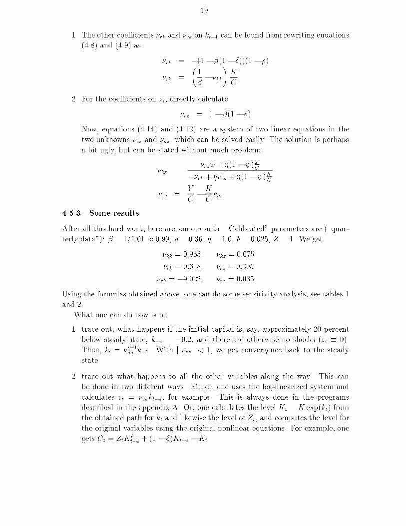
�� The other coe�cients �rk and �ck on kt�� can be found from rewriting euuations

� �� and � �� as

�rk � ��

�ck �

��

�� kk

��K�C

�� For the coe�cients on zt� directly calculate

�rz � ��

Now� equations � �� and � �� are a system of two linear equations in the

two unknowns �cz and �kz� which can be solved easily� The solution is perhaps

a bit ugly� but can be stated without much problem�

�kz ��rz � ��

�Y�C

��rk � ��ck � �� K�C

�cz ��Y�C��K�C�kz

�� Some results

After all this hard work� here are some results� �Calibrated� parameters are ��quar�

terly data�� Z � �� We get�kk � �� kz � ��

�ck � �� cz � ��

�rk � �� rz � ��

Using the formulas obtained above� one can do some sensitivity analysis� see tables �

and ��

What one can do now is to

�� trace out� what happens if the initial capital is� say� approximately �� percent

below steady state� k�� and there are otherwise no shocks �zt � ��

Then� kt � �t��kk k�� With j �kk j� �� we get convergence back to the steady

state�

�� trace out what happens to all the other variables along the way� This can

be done in two di�erent ways� Either� one uses the log�linearized system and

calculates ct � �ckkt�� for example� This is always done in the programs

described in the appendix A� Or� one calculates the level Kt � �K exp�kt� from

the obtained path for kt and likewise the level of Zt� and computes the level for

the original variables using the original nonlinear equations� For example� one

gets Ct � ZtK�t�� Kt�� Kt�

��

�kk � � � ��

� � � ��

� � ��

� � ��

� � ��

Table �� Some sensitivity analysis in the neoclassical growth model� If depreciation �

is less or if the intertemporal elasticity of substitution �� is smaller� the speed ��kkof convergence back to the steady state is slower�

�kz � � � ��

� � � ��

� � ��

� � ��

� � ��

Table �� Some sensitivity analysis in the neoclassical growth model� If depreciation �

is less or if the intertemporal elasticity of substitution �� is smaller� the reaction �kzof the new capital stock� i�e� of investment� is generally smaller too� except for very

low levels of �� compare the last two columns��

��

� simulate the model� simulate �ts� pick some initial k�� and z�� Then� calculate

recursively

zt � zt�� t

kt � �kkkt�� kzzt�

With that� obtain all other variables�

� trace out what happens to all the variables after � � �� t � � for t � �� when

starting from the steady state� This is called an impulse response analysis�

Impulse responses for the neoclassical growth model are shown in �gure ��

0 2 4 6 8−0.2

0

0.2

0.4

0.6

0.8

1Impulse responses to shock in technology

Years after shock

Per

cent

dev

iatio

n fr

om s

tead

y st

ate

capital

consumption

return

output technology

Figure �� This �gure shows the impulse response for the stochastic neoclassical growth

model� The parameters are as stated in the text�

�� The relationship to a state�space approach�

In this section� we will discuss the popular reduction to a system in ct and kt�� for

the log�linearized system or to a system in Ct and Kt�� in the original system� this

��

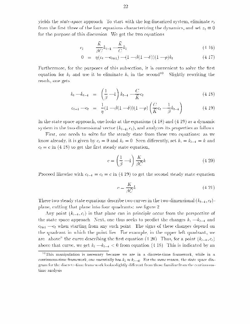
yields the state�space approach� To start with the log�linearized system� eliminate rtfrom the �rst three of the four equations characterizing the dynamics� and set zt � �for the purpose of this discussion� We get the two equations

ct ��K

� �Ckt��

�K�Ckt � ��

� � ��ct � ct�� kt � ��

Furthermore� for the purposes of this subsection� it is convenient to solve the �rst

equation for kt and use it to eliminate kt in the second�� Slightly rewriting the

result� one gets

kt � kt��

��

��

�kt��

�C�Kct � ��

ct�� ct ��

��

��C�Kct � �

�kt��

��

In the state space approach� one looks at the equations � �� and � �� as a dynamic

system in the two�dimensional vector �kt�� ct�� and analyzes its properties as follows�

First� one needs to solve for the steady state from these two equations� as we

know already� it is given by ct � � and kt � �� Seen di�erently� set kt � kt�� k and

ct � c in � �� to get the �rst steady state equation�

c �

��

��

��K

� �Ck � ��

Proceed likewise with ct�� ct � c in � �� to get the second steady state equation

c ��K

� �Ck � ��

These two steady state equations describe two curves in the two�dimensional �kt�� ct��

plane� cutting that plane into four quadrants� see �gure ��

Any point �kt�� ct� in that plane can in principle occur from the perspective of

the state space approach� Next� one thus seeks to predict the changes kt � kt�� and

ct�� ct when starting from any such point� The signs of these changes depend on

the quadrant in which the point lies� For example� in the upper left quadrant� we

are �above� the curve describing the �rst equation � �� Thus� for a point �kt�� ct�

above that curve� we get kt � kt�� from equation � �� This is indicated by an

��This manipulation is necessary because we are in a discrete�time framework� while in a

continuous�time framework� one essentially has kt � kt�dt� For the same reason� the state space dia�

gram for the discrete�time framework looks slightly di�erent from those familiar from the continuous�

time analysis�

�

−10 −8 −6 −4 −2 0 2 4 6 8 10−10

−8

−6

−4

−2

0

2

4

6

8

10

k(t−1) in Percent

c(t)

in P

erce

nt

Neoclassical growth model: State Space Diagram (Log−Deviations)

First steady state equation

Second steady state equation

Stable arm

Figure �� This �gure shows the state space diagram for the log�linearized neoclassical

growth model� The two steady state equations cut the plane into four quadrants�

which dier qualitatively in their dynamics as indicated by the arrows at right angles�

The stable arm is the function ct � �ckkt�� which was derived with the method of

undetermined coecients�

arrow pointing to the left� Furthermore� in the upper left quadrant� we are �to the

left� of the curve describing the second equation � �� Thus� for a point �kt�� ct� to

the left of that curve� we get ct��ct � � from equation � �� Thus� consumption is

increasing there� indicated by the arrows pointing upwards� In this manner� one can

analyze the dynamic behaviour at every point in the plane� Looking at these arrows�

one can see that the system is saddle�point stable� it diverges away from the origin

in the upper left quadrant and the lower right quadrant� and may have a chance to

converge towards it in the lower left quadrant and the upper right quadrant� Finally�

one can trace out trajectories of the dynamic system� starting it at any point �kt�� ct�

and letting it evolve according to the equations � �� and � �� It turns out that

these trajectories will converge to the steady state k � �� c � �� if and only if the

�

trajectories were started from a point on the stable arm� Further analysis reveals� that

the stable arm is given by ct � �ckkt�� In other words� the method of undetermined

coe�cients delivers the calculation of the stable arm for saddle�point stable systems�

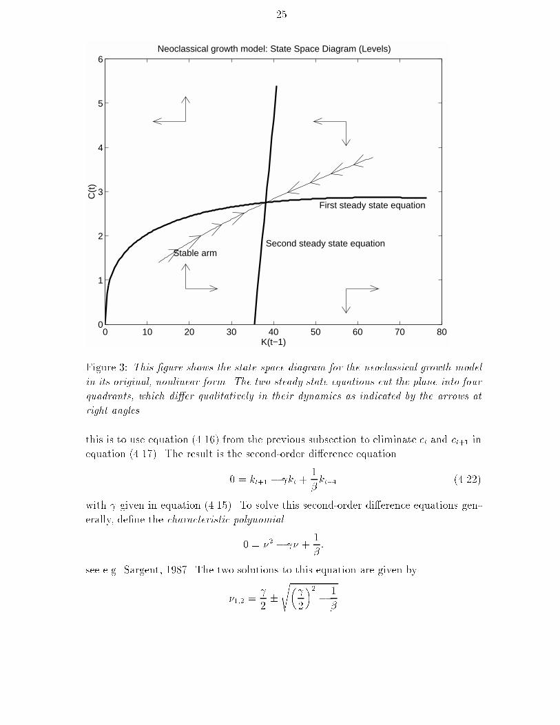
Rather than looking at the system in log�deviation form� one can also look at the

original� nonlinear system and reduce it to a system in Ct and Kt�� setting Zt � �Z

for the sake of this argument�

Ct � �ZK�t�� Kt�� Kt

� � �

�Ct

Ct��

�� ZK��

t � ��

As above� solve the �rst equation for Kt and use the result to replaceKt in the second

equation�� yielding with slight rewriting

Kt �Kt�� ZK�t�� Kt�� Ct

Ct��

Ct�

�� Z

��ZK�

t�� Kt�� Ct

��

��

Again� one obtains two steady state relationships for Kt�� Kt � K and Ct��

Ct � C�

C � �ZK� � �K

C � �ZK� � �� K ��

� �Z

��

��

These two relationships can be plotted into the �Kt�� Ct��plane� dissecting that plane

into four quadrants� see �gure � The analysis proceeds exactly as above� As stable

arm� we have used the relationship Ct � �C exp��ck log�Kt�� K�� which according to

our log�linear analysis is approximately correct�

The state�space approach is certainly useful for gaining insights into small systems

such as the neoclassical growth model we have studied here� However� for larger

models� it becomes impractical very quickly�

�� The relationship to second�order dierence equations�

In this subsection� we will discuss the popular reduction to a second�order dierence

equation� Further discussion can also be found in subsection �� As in the previous

subsection� we ignore the stochastic term zt for the purpose of the discussion here

by setting it identical to zero� The four log�linearized equations characterizing the

dynamics can be reduced to a single second�order equation in kt� One way of seeing

��Again� this manipulation is not necessary in a continuous�time framework�

��

0 10 20 30 40 50 60 70 800

1

2

3

4

5

6

K(t−1)

C(t

)

Neoclassical growth model: State Space Diagram (Levels)

First steady state equation

Second steady state equationStable arm

Figure � This �gure shows the state space diagram for the neoclassical growth model

in its original� nonlinear form� The two steady state equations cut the plane into four

quadrants� which dier qualitatively in their dynamics as indicated by the arrows at

right angles�

this is to use equation � �� from the previous subsection to eliminate ct and ct�� in

equation � �� The result is the second�order di�erence equation

� � kt�� kt ��

�kt��

with � given in equation � �� To solve this second�order di�erence equations gen�

erally� de�ne the characteristic polynomial

� � ��

��

see e�g� Sargent� �� The two solutions to this equation are given by

��

��s�

�

�

��

� �

�

��

We then have the following well�known proposition�

Proposition � If �� then the general solution to �� is the two�dimensional

space� given by

kt � a�t� � b�t� � ��

for arbitrary constants a and b�

Proof Suppose� kt is given by �� Substituting it into �� yields

kt�� kt ��

�kt��

� a�t��

��

�

�

�

�b�t��

��

�

�

�

� �

as desired� Conversely� let any solution to �� be given� Note� that it is enough to

just know k� and k�� say� since all other kt can then be calculated recursively from

�� Find a and b such that

k� � a� b

k� � a�� b��

There is a unique solution� since �� Then� the given solution to �� must

coincide with �� for these values of a and b�

Since the general solution to equation � �� is a two�dimensional space� one needs

two constraints to pin down a unique solution� One constraint is the initial value for

capital k�� or k�� if one starts time in the neoclassical growth model at t � �� The

second constraint is the stability condition� that

� � limt��

kt

This constraint helps� if exactly one of the roots� �� say� is stable� in that case� we

must have b � � in � �� Furthermore� we now have the recursive equilibrium law

of motion

kt � ��kt��

In other words� for second�order di�erence equations with exactly one stable root� the

method of undetermined coe�cients �nds the stable solution with �� kk�

��

Note� that the stability condition does not help� if both roots are stable� In that

case� one still has a one�dimensional space of general solutions� Such systems can give

rise to sunspot dynamics� see Farmer and Guo �� for further discussion� One then

has to be careful with the interpretation of the results of the method of undetermined

coe�cients� since that method� given one endogenous state variable� imposes the

restriction on the solution of the system to be of form � �� which is no longer

valid� A remedy is to enlarge the state space to include kt�� and kt�� the method

of undetermined coe�cients then correctly searches for a recursive equilibrium law of

motion of the type

kt � �kk�kt�� kk�kt��

with �kk� � � and �kk� � �� as a stable and simple�to��nd solution� More generally�enlarging the state space leads to more complicated matrix algebra� which is dealt

with in section �� The point here is to keep in mind� that one should be very careful�

if one �nds �too many� �or� likewise� �too few�� stable roots� when applying the

method of undetermined coe�cients�

�� A quick review�

It may be useful at this point to step back and to provide a quick review�

�� We have found the necessary conditions�

�� We log�linearized these conditions and the constraints� E�g� we got

� � Et ��ct � ct�� rt��

� We postulated a linear law of motion� e�g�

kt � �kkkt�� kzzt

and solved for the �undetermined coe�cients� �kk� �kz etc��

� It all boiled down to solving a quadratic equation for the coe�cient �kk� given

by

� � ��kk � ��kk ��

�

where � is given in equation � ��

�� The resulting equations could then be used to analyze the model by e�g� cal�

culating the coe�cient �kk for particular parameter choices� doing sensitivity

analysis with respect to these choices� analyzing the speed of convergence back

to the steady state� simulating the model or looking at impulse response func�

tions�

�

�� We have compared the method of undetermined coe�cients to a state space

approach as well as to solving second order di�erence equations�

In looking back� we can also see that �nding the necessary conditions� �nding the

steady state� as well as log�linearizing these conditions and the constraints was com�

paratively easy� Painful� however� was to have to solve for �kk and the other co�

e�cients� For larger models or� worse� for models with multiple endogenous state

variables� solving for everything by hand looks quite unattractive�

However� this pain can be avoided by applying directly the theorems in section ��

The easiest way to apply these theorems is to obtain MATLAB routines applying

them� They are described in appendix A and are available together with some docu�

mentation and examples at the following web site�

http��cwis�kub�nl��few��center�STAFF�uhlig�toolkit�dir�toolkit�htm�

� An example� Hansens real business cycle model�

The next example is Hansens �� real business cycle model� It is explained there

in detail� Here� the mathematical description shall su�ce� The main point of this

example is to explain how to perform the �rst three steps of the general procedure as

stated in section � In many ways� the model here is just an extension of the stochastic

neoclassical growth model of section above� the main di�erence is to endogenize

the labor supply� In fact� it is possible to also solve through that model by hand just

as was done above for the stochastic neoclassical growth model� However� here� we

want to go through the analysis of this model rather quickly to show how to get to

the log�linearized version of the model ready for the analysis with the theorems of

section � and the MATLAB programs mentioned there�

The social planner solves the problem of the representative agent

maxE�Xt��

�t�C��t � ��

�ANt

�

s�t�

Ct � It � Yt ��

Kt � It � �� Kt��

Yt � ZtK�t��N

��t

log Zt � �� log �Z � logZt�� t� t � i�i�d�N ��

where Ct is consumption� Nt is labor�It is investment� Yt is production� Kt is capital Zt

��

is the total factor productivity and A�� Z� and �� are parameters� Hansen

only considered the case � � �� so that the objective function is

E�Xt��

�t�logCt �ANt�

As in Campbell �� there is no di�culty in considering arbitrary �� since no

growth trend is assumed�

The �rst order conditions are

A � C��t �� YtNt

� � �Et

��Ct

Ct��

��

Rt��

��

Rt � �Yt

Kt��

Equation �� is the Lucas asset pricing equations� see Lucas �� which typically

arises in these models�

In contrast to some of the real business cycle literature and to avoid confusion in

the application of the method in section �� it is very useful to stick to the following

dating convention� A new date starts with the arrival of new information� If a variable

is chosen and�or �eventually� known at date t� it will be indexed with t� Use only

variables dated t and t� � in deterministic equations and variables dated t�� t andt� � in equations involving expectations Et��The steady state for the real business cycle model above is obtained by drop�

ping the time subscripts and stochastic shocks in the equations above� characterizing

the equilibrium� Formally� this amounts to �nding steady state values such that

f�� and g�� in the notation of the previous section�� For example�

equations �� and �� result in

� � � �R

�R � ��Y�K� ��

where bars over variables denote steady state values� One needs to decide what one

wants to solve for� If one �xes � and �� these two equations will imply values for �R and�Y � �K � Conversely� one can �x �R and �Y � �K and then these two equations yield values

for � and �� The latter procedure maps observable characteristics of the economy

into �deep parameters�� and is the essence of calibration� see Kydland and Prescott

��

��Alternatively� �nd the steady state so that �� is satis�ed� This is� however� rarely done�

�

Introduce small letters to denote log�deviations� i�e� write

Ct � �Cect

for example� The resource constraint �� then reads

�Cect � �Ieit � �Y eyt

This can be written approximately as

�C�� ct� � �I�� it� � �Y �� yt�

Since �C � �I � �Y due to the de�nition of the steady state� the constant terms drop

out�� and one obtains�Cct � �Iit � �Y yt ��

The resource constraint is now stated in terms of percentage deviations� the steady

state levels in this equation rescale the percentage deviations to make them compa�

rable� Note that no explicit di�erentiation is required to obtain the log�linearized

version of the resource constraint� log�linearization is obtained just by using the

building blocks described in the previous section�

Similarly log�linearizating the other equations yields

�Kkt � �Iit � �� Kkt��

yt � zt � �kt�� nt

zt � zt�� t

� � ��ct � yt � nt

� � Et��ct � ct�� rt��

�Rrt � ��Y�K�yt � kt��

To �nd the state variables� one needs to �nd all �linear combinations of� variables

dated t� � in these equations� the endogenous state variable is capital� kt�� whereasthe exogenous state variable is the technology parameter zt�� Note that there are as

many expectational equations as there are endogenous state variables� The coe�cients

of the equations above need to be collected in the appropriate matrices to restate these

equations in the form required for section �� this is a straightforward exercise�

��Another way to see that constants can in the end be dropped is to note that the steady state

is characterized by ct � kt � yt � kt�� If one replaces all log�deviations with zero� only the

constant terms remain� and that equation can be subtracted from the equation for general ct� kt� ytand kt�� above�

�

Solving recursive stochastic linear systems with

the method of undetermined coecients

This section describes how to �nd the solution to the recursive equilibrium law of

motion in general� using the method of undetermined coe�cients� MATLAB pro�

grams performing the calculations in this section are available at my home page��

The idea is to write all variables as linear functions �the �recursive equilibrium law of

motion�� of a vector of endogenous variables xt�� and exogenous variables zt� which

are given at date t� i�e� which cannot be changed at date t� These variables are often

called state variables or predetermined variables� In the real business cycle example

of section �� these are at least kt�� and zt� since they are clearly unchangeable as of

date t and� furthermore� show up in the linearized equations system� In principle�

any endogenous variable dated t � � or earlier could be considered a state variable�Thus� in subsection �� below� we use �brute force� and simply declare all endoge�

nous variables to be state variables� whereas in subsection �� we try to be a bit more

sensitive and exploit more of the available structure� The latter is typically done in

practice� see e�g� Campbell �� Both subsections will characterize the solution

with a matrix quadratic equation� see also Ceria and Rios�Rull �� and Binder

and Pesaran �� Subsection �� shows� how to solve that equation� For models

with just one endogenous state variable� such as the real business cycle model of

section � when analyzed with the more structured approach in subsection �� below�

the matrix quadratic equation is simply a quadratic equation in a real number� In

that case� the solution to the quadratic equation is obviously known from high�school

algebra� it is contained as a special case of the general solution in section �� In

subsection �� we discuss our solution method� and compare it in particular to the

Blanchard�Kahn �� approach�

�� With brute force��

As a �rst cut� and with somewhat brute force� one may simply use all variables

without distinction as a vector of endogenous state variables�� xt�� of size m� � oras a vector of exogenous stochastic processes zt of size k � �� It is assumed that thelog�linearized equilibrium relationships can be written in the following form

� � Et�Fxt�� Gxt �Hxt�� Lzt�� Mzt� ��

��http��cwis�kub�nl��few��center�STAFF�uhlig�toolkit�dir�toolkit�htm is the address of the

web site for the programs��To make this work really generally� one should actually not only include all the variables dated

t � but also all the variables dated t � � as part of the state vector xt�� More is even required�

if the equations already contain further lags of endogenous variables� see also the next footnote�

Usually� however� this isn�t necessary�

�

zt�� Nzt � t�� Et�t��

where F � G� H� L and M and matrices� collecting the coe�cients� It is assumed that

N has only stable eigenvalues� The real business cycle example above can be easily

written in this form� For example� the resource constraint �� would be

� � Et� �Cct � �Iit � �Y yt�

since ct� it and yt are already known at date t and hence nothing changes when one

takes their expectations given all information up to date t� Note that F � L � � for

this equation� Of course� there are other equations in the real business cycle model�

and one of them involves nonzero entries for F and L�

What one is looking for is the recursive equilibrium law of motion

xt � Pxt�� Qzt ��

i�e� matrices P and Q � so that the equilibrium described by these rules is stable� The

solution is characterized in the following theorem� see also Binder and Pesaran ��

The characterization involves a matrix quadratic equation� see equation �� Sub�

section �� discusses� how it can be solved� For the purpose of that section� let m be

the length of the vector xt� and let l � n � ��

Theorem � If there is a recursive equilibrium law of motion solving equations � ��

and � �� then the following must be true�

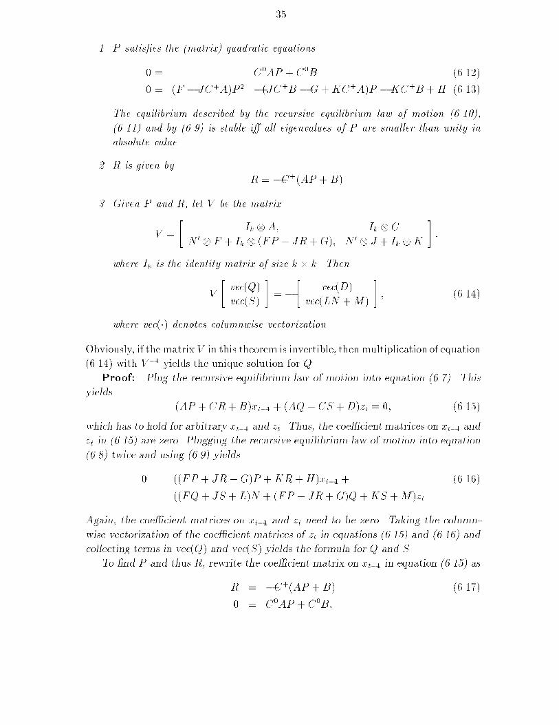
�� P satis�es the �matrix� quadratic equation

� � FP � �GP �H ��

The equilibrium described by the recursive equilibrium law of motion � �� and

� �� is stable i all eigenvalues of P are smaller than unity in absolute value�

�� Given P � let V denote the matrix

V � N � � F � Ik � �FP �G��

Then�

V Q � �vec�LN �M� ��

where vec�� denotes columnwise vectorization�

Obviously� if the matrix V in this theorem is invertible� then multiplication of equation

�� with V �� yields the unique solution for Q� Proof Plugging the recursive

equilibrium law of motion �� into equation �� twice and using �� to calculate

the expectations yields

� � ��FP �G�P �H�xt��

��FQ� L�N � �FP �G�Q�M�zt

The coecient matrices on xt�� and zt need to be zero� Equating the coecient on

xt�� to zero yields equation �� for P � Taking the columnwise vectorization of the

coecient matrices of zt in this equation and collecting terms in vec�Q� yields the

equation �� for Q�

�� or with sensitivity�

We now exploit more of the structure in the linearized model� Analyzing the equations

of the real business cycle example of section �� one sees that the only endogenous

variable dated t � � which shows up in any of the equations is capital� kt�� It isthus a reasonably guess to treat kt�� as the only endogenous state variable together

with the exogenous state variable zt� This principle is general� in the vast majority

of cases� this is how one can identify the vector of state variables�� In practice�

one often sees researchers exploiting some of the equilibrium equations to �get rid�

of some variables� and have only a few variables remaining� For the real business

cycle example of section �� it is actually possible to reduce everything to a single

equation for the endogenous variables� containing only kt�� kt and kt�� Often� one

sees reductions to a system involving two equations in two endogenous variables such

as ct and kt�� see e�g� Campbell �� presumably because this allows thinking in

terms of a state space diagram� see e�g� Blanchard and Fisher �� chapter �� The

analysis below follows this often�used procedure� However� there is no reason to go

through the hassle of �eliminating� variables by hand� using some of the equations�

since this is all just simple linear algebra applied to a system of equations� it is far

�There are exceptions� In richer models� the state variables need to include variables chosen at

a date earlier than t � as well because these lagged variables appear in the equations� One can

recast this into the desired format as follows� The list of state variables might consist out of lagged

values of the capital stock� kt�� and kt�� This can and should be rewritten as k��t�� and k��t��

with k��t�� replacing kt�� and where the additional equation k��t � k��t�� needs to be added to the

system� With that notation� k��t is �chosen� at date t� satisfying the �dating convention� stated in

section �� One may also need to add additional variables like e�g� ct�� or kt�� as state variables�

even though they don�t show up in the equations with these dates� when the model exhibits sun

spot dynamics� This can be done in the same manner� but one needs to be careful with interpreting

the results� The reader is advised to read Farmer and Guo �� for an example as well for the

appropriate interpretation for such a case�

easier to leave all the equations in� and leave it to the formulas to sort it all out� That

is what is done below�

We thus make the following assumptions�� There is an endogenous state vector

xt� sizem�� a list of other endogenous variables ��jump variables�� yt� size n�� anda list of exogenous stochastic processes zt� size k � �� The equilibrium relationshipsbetween these variables are

� � Axt �Bxt�� Cyt �Dzt ��

� � Et�Fxt��Gxt �Hxt�� Jyt�� Kyt � Lzt�� Mzt� ��

zt�� Nzt � t�� Et�t��

where it is assumed that C is of size l � n� l n and� of rank n� that F is of

size �m � n � l� � n� and that N has only stable eigenvalues� Note� that one could

have written all equations �� in the form of equation �� with the corresponding

entries in the matrices F � J and L set to zero� Essentially� that is what is done in

subsection �� Instead� the point here is to somehow exploit the structure inherent

in equations of the form �� which do not involve taking expectations�

What one is looking for is the recursive equilibrium law of motion

xt � Pxt�� Qzt ��

yt � Rxt�� Szt� ��

i�e� matrices P�Q�R and S� so that the equilibrium described by these rules is stable�

The solution is characterized in the next theorem� To calculate the solution� one needs

to solve a matrix quadratic equation� how this is done� is explained in subsection ��

The important special case l � n is treated in corrolary �� The special case

l � n � � was the topic of subsection ��

Theorem � If there is a recursive equilibrium law of motion solving equations � ��

� �� and � �� then the coecient matrices can be found as follows� Let C� be the

pseudo�inverse�� of C� Let C� be an �l � n� � l matrix� whose rows form a basis of

the null space�� of C ��

�Note that the notation di�ers from the notation in section ��The case l � n can be treated as well� the easiest approach is to simply �redeclare� some other

endogenous variables to be state variables instead� i�e� to raise m and thus lower n� until l � n��The pseudo�inverse of the matrix C is the n � l matrix C� satisfying C�CC� � C� and

CC�C � C� Since it is assumed that rank�C� � n� one gets C� � �C�C��C�� see Strang ��

p� �� The MATLAB command to compute the pseudo�inverse is pinv�C��C� can be found via the singular value decomposition of C�� see Strang �� p� �� The

MATLAB command for computing C� is �null�C��

�

�� P satis�es the �matrix� quadratic equations

� � C�AP � C�B ��

� � �F � JC�A�P � ��JC�B �G �KC�A�P �KC�B �H ��

The equilibrium described by the recursive equilibrium law of motion � ��

� �� and by � �� is stable i all eigenvalues of P are smaller than unity in

absolute value�

�� R is given by

R � �C��AP �B�

�� Given P and R� let V be the matrix

V �

�Ik �A� Ik � C

N � � F � Ik � �FP � JR�G�� N � � J � Ik �K

��

where Ik is the identity matrix of size k � k� Then

V

�vec�Q�

vec�S�

��

�vec�D�

vec�LN �M�

��

where vec�� denotes columnwise vectorization�

Obviously� if the matrix V in this theorem is invertible� then multiplication of equation

�� with V �� yields the unique solution for Q�

Proof Plug the recursive equilibrium law of motion into equation �� This

yields

�AP � CR�B�xt�� AQ� CS �D�zt � ��

which has to hold for arbitrary xt�� and zt� Thus� the coecient matrices on xt�� and

zt in �� are zero� Plugging the recursive equilibrium law of motion into equation

�� twice and using �� yields

� � ��FP � JR �G�P �KR �H�xt��

��FQ� JS � L�N � �FP � JR �G�Q�KS �M�zt

Again� the coecient matrices on xt�� and zt need to be zero� Taking the column�

wise vectorization of the coecient matrices of zt in equations �� and �� and

collecting terms in vec�Q� and vec�S� yields the formula for Q and S�

To �nd P and thus R� rewrite the coecient matrix on xt�� in equation �� as

R � �C��AP �B� ��

� � C�AP � C�B�

�

noting that the matrix ��C�� C�� is nonsingular and that C�C � �� see Strang ��

p� � Use �� to replace R in the coecient matrix on xt�� in �� yielding

�� Note �nally that the stability of the equilibrium is determined by the stability

of P � since N has stable roots by assumption�

Corollary � Suppose that l � n� i�e� that there are as many expectational equations

as there are endogenous state variables� If there is a recursive equilibrium law of

motion solving equations � �� and � �� then their coecient matrices can be

found as follows�

�� P satis�es the �matrix� quadratic equation

�F � JC��A�P � � �JC��B �G�KC��A�P �KC��B �H � ��

The equilibrium described by the recursive equilibrium law of motion � ��

� �� and by � �� is stable i all eigenvalues of P are smaller than unity in

absolute value�

�� R is given by

R � �C��AP �B�

�� Q satis�es

�N � � �F � JC��A� � Ik � �JR� FP �G�KC��A��vec�Q� �

vec��JC��D � L�N �KC��D �M��

where Ik is the identity matrix of size k� k� provided the matrix which needs to

be inverted in this formula is indeed invertible�

�� S is given by

S � �C��AQ�D�

Proof This corollary can be obtained directly by inspecting the formulas of the�

orem � above for the special case l � n� In particular� C� is just the inverse of C�

Alternatively� a direct proof can be obtained directly by following the same proof

strategy as above� there is no need to repeat it�

The formulas in these theorems become simpler yet� if m � � or k � �� If

m � �� there is just one endogenous state variable and the matrix quadratic equation

�

above becomes a quadratic equation in the real number P � which can be solved using

high�school algebra� this is the case for the real business cycle model and thus the

case which Campbell �� analyzes� If k � �� there is just one exogenous state

variables� in which case the Kronecker product �i�e� �� in the formulas abovebecomes multiplication� and in which case vec�Q� � Q and vec�S� � S� since Q and

S are already vectors rather than matrices�

�� Solving the matrix quadratic equation�

To generally solve the matrix quadratic equations �� or �� for P � write

them generally as

�P � � �P � � ��

For equations �� and �� de�ne

� �

��l�n�m

F � JC�A

�

� �

�C�A

JC�B �G �KC�A

�

�

�C�B

KC�B �H�

�

where �l�n�m is a �l� n��m matrix with only zero entries� In the special case l � n�

the formulas for �� and become slightly simpler�

� � F � JC��A

� � JC��B �G �KC��A

� KC��B �H

For equation �� simply use � � F � � � �G and � �H�Equation �� can now be solved by turning it into a generalized eigenvalue and

eigenvector problem�� for which most mathematical packages have preprogrammed

routines�� Recall� that a generalized eigenvalue � and eigenvector s of a matrix !

with respect to a matrix " are de�ned to be a vector and a value satisfying

�"s � !s ��

��An earlier version of the chapter proposed to study an altered version of these equations by

postmultiplying equation �� with P � This altered equation together with �� can then often

be reduced to a standard rather than a generalized eigenvalue problem� but had the drawback of

introducing spurious zero roots� The version presented here does not involve this alteration� and

thus does not introduce spurious zero roots� This update is due to Andy Atkeson �� and I am

very grateful to him for pointing it out to me� Any errors here are mine� of course��The Matlab command for �nding the generalized eigenvalues and eigenvectors is eig��

A standard eigenvalue problem is obtained� if " is the identity matrix� More gener�

ally� the generalized eigenvector problem can be reduced to a standard one� if " is

invertible� by calculating standard eigenvalues and eigenvectors for "��! instead�

Theorem � To solve the quadratic matrix equation

�P � � �P � � ��

for the m�m matrix P � given m�m matrices � and � de�ne the �m��m matrices

! and " via

! �

��

Im �m�m

��

and

" �

�� m�m

�m�m Im

��

where Im is the identity matrix of size m� and where �m�m is the m�m matrix with

only zero entries�

�� If s is a generalized eigenvector and � the corresponding generalized eigenvalue

of ! with respect to "� then s can be written as s� � ��x�� x�� for some x � IRm�

�� If there are m generalized eigenvalues �� m together with generalized eigen�

vectors s�� sm of ! with respect to "� written as s�i � ��ix�i� x�

i� for some

xi � IRm� and if �x�� xm� is linearly independent� then

P � #$#��

is a solution to the matrix quadratic equation � �� where # � �x�� xm� and

$ � diag�� m�� The solution P is stable if j �i j� � for all i � �� m�

Conversely� any diagonalizable solution P to � �� can be written in this way�

�� If m � �� then the solutions P to equation � �� are given by

P��

��p��

if � � � and

P � � �

if � � � and � � ��

�

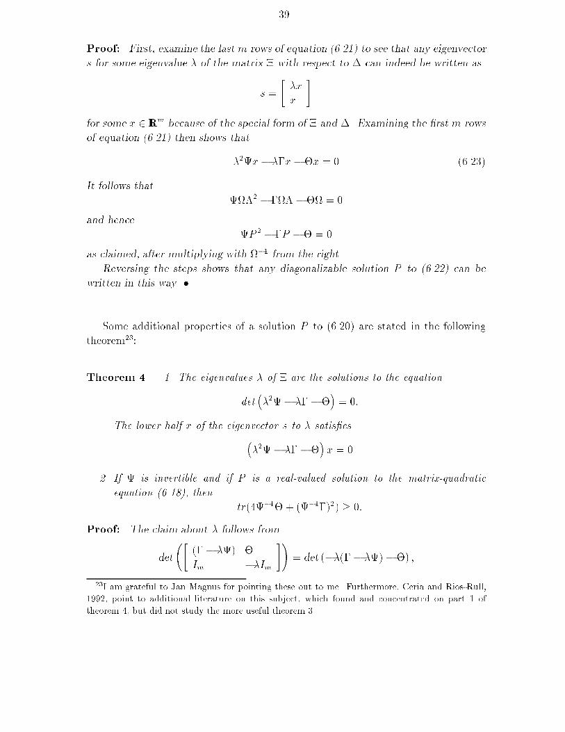
Proof First� examine the last m rows of equation �� to see that any eigenvector

s for some eigenvalue � of the matrix ! with respect to " can indeed be written as

s �

��x

x

�

for some x � IRm because of the special form of ! and "� Examining the �rst m rows

of equation �� then shows that

��x� ��x� x � � ��

It follows that

�#$� � �#$ � # � �and hence

�P � � �P � � �as claimed� after multiplying with #�� from the right�

Reversing the steps shows that any diagonalizable solution P to �� can be

written in this way�

Some additional properties of a solution P to �� are stated in the following

theorem��

Theorem � �� The eigenvalues � of ! are the solutions to the equation

det��

��

The lower half x of the eigenvector s to � satis�es��

�x � �

�� If � is invertible and if P is a real�valued solution to the matrix�quadratic

equation � �� then

tr� �� Proof The claim about � follows from

det

��

Im ��Im

�� det ��

��I am grateful to Jan Magnus for pointing these out to me� Furthermore� Ceria and Rios�Rull�

�� point to additional literature on this subject� which found and concentrated on part of

theorem �� but did not study the more useful theorem ��

�

which follows from inspecting the formula for the determinant� The claim about the

eigenvector piece x is just �� For the last claim� calculate that

� � tr�P � ��P �� tr��P � ��

��

The conclusion follows since tr��P � ��

��

�� Discussion�

Theorem links the approach used here to Blanchard and Kahn �� which is

the key reference for solving linear di�erence equations� Consider solving the second

order di�erence equation

�xt�� xt � xt��

The approach in Blanchard and Kahn �� amounts to �nding the stable roots of

! by instead analyzing the dynamics of the �stacked� system s�t � �x�

t� x�

t��

"st�� !st�

i�e� by reducing �� to a �rst�order di�erence equation� The approach here solves

for the matrix P in the recursive equilibrium law of motion xt�� Pxt� Theorem

above states that both approaches amount to the same problem� The advantage of

the method here is that it is easily applied to the entire system �� and ��

reducing it to �� eventually� while �nding the stable roots in the entire system

given by these equations and at the same time taking care of the expectation opera�

tors� using the Blanchard�Kahn �� procedure� is often perceived as complicated�

Fundamentally� there is no di�erence�

To apply theorem � one needs to select m out of �m possible eigenvalues� Note

that P has only nonzero eigenvalues if the state space was chosen to be of minimal

size� thus attention can be restricted to the roots j �i j� � in that case� In gen�

eral� there may be quite a bit of choice left� In practice� however� there will often

be exactly m stable eigenvalues remaining so that the stable solution is unique��

��Another approach to select a unique solution is in McCallum �� who suggests to use those

roots that can be obtained continuously from the zero roots of the equation P � � !P � �" for

� � � as � changes from to � However� not only is following these roots as functions of �

computationally very demanding� it is also the case that uniqueness gets lost once two or more such

paths cross each other� If these paths do not cross in a particular application� and if additionally

all roots for all � are positive real numbers� say� then the McCallum proposal simply amounts to

using the roots of minimal value� The MATLAB programs supplied by the author use the roots of

minimal absolute value subject to eliminating spurious zero roots and tries to use complex roots in

conjugate pairs� as described below�

�

For a one�dimensional vector of endogenous state variables� this condition is called

saddle�point stability� The literature on solving linear rational expectations equilibria

typically assumes this condition to hold or shows it to hold in social planning prob�

lems under reasonable conditions� see Blanchard and Kahn �� Kollintzas ��

and Hansen� McGrattan and Sargent �� If there are fewer stable eigenvalues

than endogenous state variables� the equilibrium might be inherently unstable� The

method above then still permits calculation of an equilibrium which satis�es the non�

linear equilibrium conditions at least locally� In particular� in models involving more

than one agent or sectors or countries� one may �nd as many unit roots as there are

more agents �sectors� countries� than one since shocks may a�ect the relative wealth

�capital� of any two agents �sectors� countries� and thus may result in permanent

changes in their consumption paths �or capital stocks�� in these cases� the method

above allowing for unit roots still gives useful results� which obviously should then be

used with some care� These unit roots typically already show up as an indetermined

steady state� any of the possible steady states can then serve as a starting point for

the dynamic calculation� keeping in mind that a simulation based on the dynamics

calculated here will eventually wander away too far to be numerically useful� If there

are more stable eigenvalues than endogenous state variables� enlarging the number of

endogenous state variables by including further lagged values might help� Nonethe�

less� the presence of an excess of stable roots then may point to the existence of

sunspots or endogenous %uctuations� see e�g� Farmer and Guo ��

If not all eigenvalues of ! are distinct� P in turn might have repeated eigenvalues�

Since the eigenspace for a repeated eigenvalue is �usually� multidimensional� there

will be in�nitely many choices for the eigenvectors and hence in�nitely many choices

for P in that case� Note� for example� that for any given � and any three real numbers

a� b� c satisfying a� � bc � �� all matrices

P �

�a b

c �a�

solve

P � ��

� ��

��

These cases are rare in practice� since ! is diagonalizable with distinct eigenvalues

generically in the coe�cients of the system �� and ��

More disconcerting is the possibility that some of the roots may be complex rather

than real� Consider� for example� � � I�� I� and

�

��

��

��

�

Using the theorem above� one obtains exactly two stable roots� which happen to

be complex� �� i � ��e��i� where where � � �� Their associatedeigenvectors are complex� too� Calculating P results in a matrix with only real entries�

however� given by

P �

��

��

��

�cos� sin�

� sin� cos�

��

Since ! is a real�valued matrix� complex eigenvalues only arise in complex�conjugate

pairs� When using both roots of a complex�conjugate pair to calculate $ and thus

P � the resulting solution should be a real�valued matrix� In order to do this� one

may have to enlarge the state space of endogenous state variables to be at least two�

dimensional� see again Farmer and Guo �� for an example� The complex roots

then give rise to endogenous damped cycles of frequency ��

� Interpreting the results

The results obtained� i�e� the recursive equilibrium law of motion

xt � Pxt�� Qzt

yt � Rxt�� Szt

zt � Nzt�� t

can be used to examine model implications� Since xt� yt and zt are log�deviations�

the entries in P�Q�R� S and N can be understood as elasticities and interpreted

accordingly� see e�g� Campbell ��

Impulse responses to a particular shock � can be calculated by setting x� � �� y� �

� and z� � �� as well as t � � for t �� and recursively calculating zt and then xtand yt� given xt�� yt�� zt�� and t for t � �� T with the recursive equilibrium law

of motion and the law of motion for zt� This was already described for the stochastic

neoclassical growth model in subsubsection �� For the real business cycle model

of section �� the impulse response functions �excluding the response of investment�

since it reacts quite strongly� to a technology shock can be seen in �gure �

To �nd the second moment properties of the model such as variances and autocor�

relations of certain variables as well as the small sample properties of their estimators�

simulation methods are often used� Before calculating these moments� the Hodrick�

Prescott �lter is typically applied �short� HP�Filter�� This section demonstrates a

0 2 4 6 8−0.5

0

0.5

1

1.5

2Impulse responses to shock in technology

Years after shock

Per

cent

dev

iatio

n fr

om s

tead

y st

ate

capital consumption

output

labor

interest

technology

Figure � Impulse responses for Hansens �� real business cycle model� using his

parameters�

frequency�domain technique to obtain these moments �albeit without the small sam�

ple properties of their estimators� without the need for any simulations�� Obviously�

the methods here do not deliver properties of the small sample distribution� which

may be necessary for testing�

The matrix�valued spectral density for �x�t� z�t�� is given by

f��

��

��Im � Pe�i��Q

Ik

��Ik �Ne�i��&

�Ik �N �ei��hQ��Im � P �ei�� Ik

i

where Ik and Im are the identity matrices of dimension k and m� see Hamilton ��

formula �� Two ways to calculate the matrix�valued spectral density for the

��Some of these methods were originally contained in an early version of Uhlig and Xu ��

but were eventually cut from that paper�

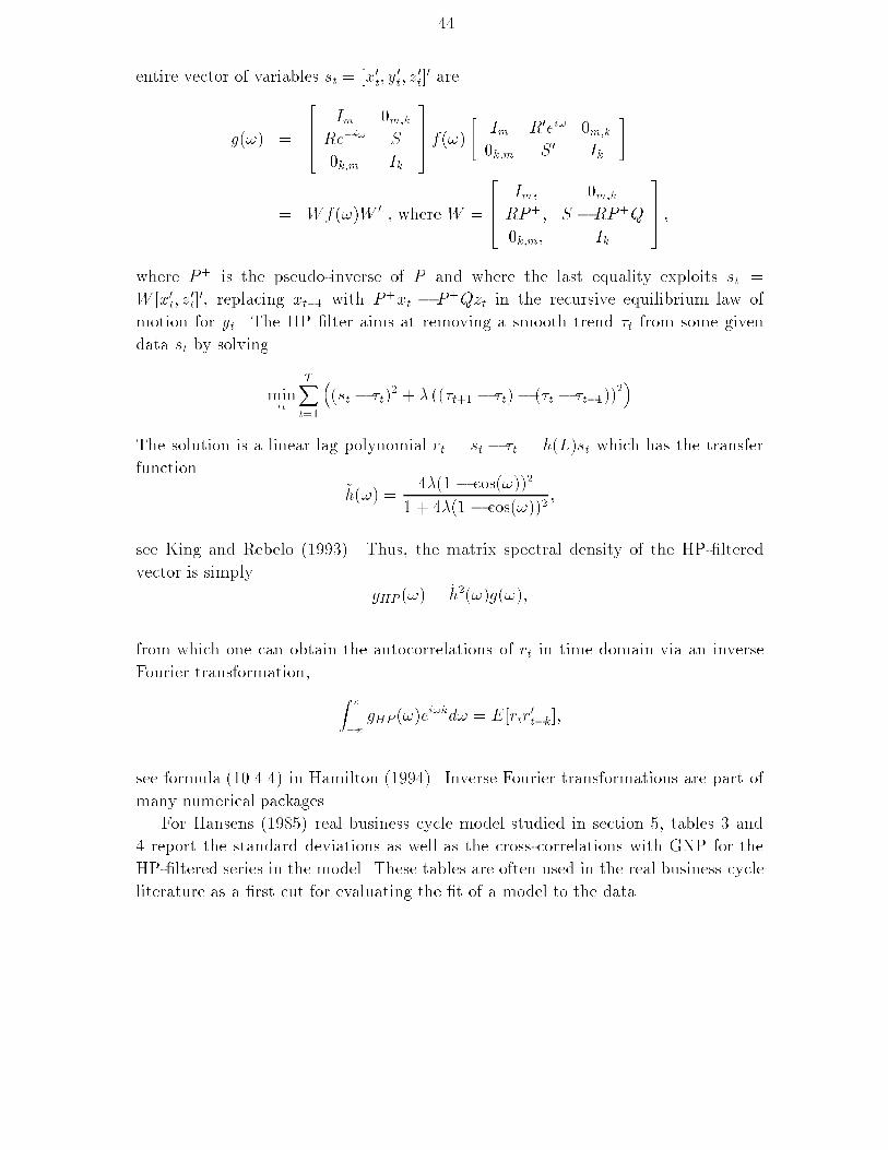
entire vector of variables st � �x�t� y�

t� z�

t�� are

g��

�

Im �m�k

Re�i� S

�k�m Ik

� � f��

�Im R�ei� �m�k

�k�m S� Ik

�

� Wf��W � � where W �

�

Im� �m�k

RP�� S �RP�Q

�k�m� Ik

� � �

where P� is the pseudo�inverse of P and where the last equality exploits st �

W �x�t� z�

t�� replacing xt�� with P�xt � P�Qzt in the recursive equilibrium law of

motion for yt� The HP �lter aims at removing a smooth trend �t from some given

data st by solving

min�t

TXt��

��st � �t�

� � � ��t�� t�� t � �t��

The solution is a linear lag polynomial rt � st � �t � h�L�st which has the transfer

function

'h�� cos��

� � �� cos��

see King and Rebelo �� Thus� the matrix spectral density of the HP��ltered

vector is simply

gHP �� 'h��g��

from which one can obtain the autocorrelations of rt in time domain via an inverse

Fourier transformation�

Z

�gHP ��e

i�kd� � E�rtr�

t�k��

see formula �� in Hamilton �� Inverse Fourier transformations are part of

many numerical packages�

For Hansens �� real business cycle model studied in section �� tables and

report the standard deviations as well as the cross�correlations with GNP for the

HP��ltered series in the model� These tables are often used in the real business cycle

literature as a �rst cut for evaluating the �t of a model to the data�

�

capital ��

consumption ��

output ��

labor ��

interest ��

investment ��

technology ��

Table � Model standard deviations of the HP��ltered series for Hansens �� real

business cycle model� studied in section ��

capital ��

consumption ��

output ��

labor ��

interest ��

investment ��

technology ��

j � ��

Table � Cross�correlations corr�v�t � j�� GNP �t�� for the HP��ltered series for

Hansens �� real business cycle model� studied in section ��

�

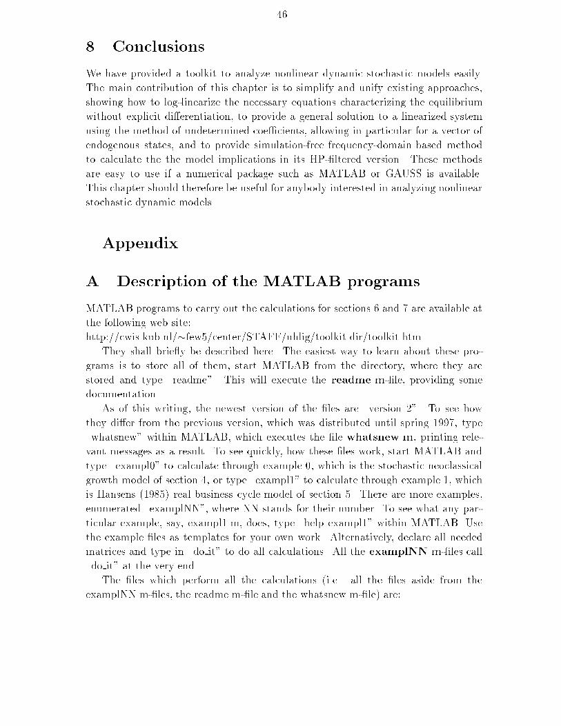
� Conclusions

We have provided a toolkit to analyze nonlinear dynamic stochastic models easily�

The main contribution of this chapter is to simplify and unify existing approaches�

showing how to log�linearize the necessary equations characterizing the equilibrium

without explicit di�erentiation� to provide a general solution to a linearized system

using the method of undetermined coe�cients� allowing in particular for a vector of

endogenous states� and to provide simulation�free frequency�domain based method

to calculate the the model implications in its HP��ltered version� These methods

are easy to use if a numerical package such as MATLAB or GAUSS is available�

This chapter should therefore be useful for anybody interested in analyzing nonlinear

stochastic dynamic models�

Appendix

A Description of the MATLAB programs�

MATLAB programs to carry out the calculations for sections � and � are available at

the following web site�

http��cwis�kub�nl��few��center�STAFF�uhlig�toolkit�dir�toolkit�htmThey shall brie%y be described here� The easiest way to learn about these pro�

grams is to store all of them� start MATLAB from the directory� where they are

stored and type �readme�� This will execute the readme�m��le� providing some

documentation�

As of this writing� the newest version of the �les are �version �� To see how

they di�er from the previous version� which was distributed until spring �� type

�whatsnew� within MATLAB� which executes the �le whatsnew�m� printing rele�

vant messages as a result� To see quickly� how these �les work� start MATLAB and

type �exampl�� to calculate through example �� which is the stochastic neoclassical

growth model of section � or type �exampl�� to calculate through example �� which

is Hansens �� real business cycle model of section �� There are more examples�

enumerated �examplNN�� where NN stands for their number� To see what any par�

ticular example� say� exampl��m� does� type �help exampl�� within MATLAB� Use

the example �les as templates for your own work� Alternatively� declare all needed

matrices and type in �do it� to do all calculations� All the examplNN�m��les call

�do it� at the very end�

The �les which perform all the calculations �i�e� all the �les aside from the

examplNN�m��les� the readme�m��le and the whatsnew�m��le� are�

�

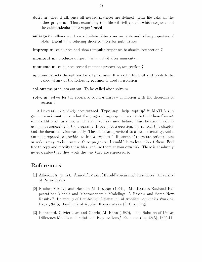
do it�m� does it all� once all needed matrices are de�ned� This �le calls all the

other programs� Thus� examining this �le will tell you� in which sequence all

the other calculations are performed�

enlarge�m� allows you to manipulate letter sizes on plots and other properties of

plots� Useful for producing slides or plots for publication�

impresp�m� calculates and shows impulse responses to shocks� see section ��

mom out�m� produces output� To be called after moments�m

moments�m� calculates second moment properties� see section ��

options�m� sets the options for all programs� It is called by do it and needs to be

called� if any of the following routines is used in isolation�

sol out�m� produces output� To be called after solve�m

solve�m� solves for the recursive equilibrium law of motion with the theorems of

section ��

All �les are extensively documented� Type� say� �help impresp� in MATLAB to

get more information on what the program impresp�m does� Note that these �les set

some additional variables� which you may have used before� thus� be careful not to

use names appearing in the programs� If you have a question� please read this chapter

and the documentation carefully� These �les are provided as a free externality� and I

am not prepared to provide �technical support�� However� if there are serious %aws

or serious ways to improve on these programs� I would like to learn about them� Feel

free to copy and modify these �les� and use them at your own risk� There is absolutely

no guarantee that they work the way they are supposed to�

References

�� Atkeson� A� �� A modi�cation of Harald(s program�� class notes� University

of Pennsylvania�

�� Binder� Michael and Hashem M� Pesaran �� Multivariate Rational Ex�

pectations Models and Macroeconomic Modeling� A Review and Some New

Results�� University of Cambridge Department of Applied Economics Working

Paper� � �� Handbook of Applied Econometrics �forthcoming��

�� Blanchard� Olivier Jean and Charles M� Kahn �� The Solution of Linear

Di�erence Models under Rational Expectations�� Econometrica� ��

� � Blanchard� Oliviers and Stanley Fisher� �� Lectures on Macroeconomics�MIT

Press�

�� Brock� W�A� and L� Mirman �� Optimal economic growth and uncertainty�

the discounted case�� Journal of Economic Theory Vol� � No� � pp� ��

�� Campbell� J� �� Inspecting the mechanism� an analytical approach to the

stochastic growth model�� Journal of Monetary Economics Vol� � No� � pp�

��

�� Campbell� J� and J� Cochrane �� By force of habit� A consumption�based

explanation of aggregate stock market behavior�� draft� Harvard University�

�� Ceria� S� and J�V� Rios�Rull �� On the Existence� Uniqueness� and Com�

putability of Nonoptimal Recursive Equilibria in Linear Quadratic Economies��

draft� Carnegie�Mellon University�

�� Danthine� J��P� and J�B� Donaldson �� Computing equilibria of nonoptimal

economics�� in T� Cooley �ed�� Frontiers of Business Cycle Research� Princeton

University Press� pp� ��

�� Farmer� Roger E� A� and Jang�Ting Guo �� Real Business Cycles and the

Animal Spirits Hypothesis�� Journal of Economic Theory ��

�� Hamilton� J�D� �� Time Series Analysis� Princeton University Press�

�� Hansen� G�D� �� Indivisible labor and the business cycle�� Journal of Mon�

etary Economics Vol� �� pp� ��

�� Hansen� G�D� and E�C� Prescott �� Recursive methods for computing equi�

libria of business cycle models�� in T�C� Cooley �ed�� Frontiers of Business Cycle

Research� Princeton University� pp� ��

�� Hansen� L�� E�R� McGrattan and T�J� Sargent �� Mechanics of forming and

estimating linear economies�� Federal Reserve Bank of Minneapolis Sta� Report

��

�� King� R�G�� C�I� Plosser and S�T� Rebelo �� Production� growth and busi�

ness cycles� technical appendix�� working paper� University of Rochester�

�� King� R�G� and S�T� Rebelo �� Low Frequency Filtering and Real Business

Cycles�� Journal of Economic Dynamics and Control vol� �� no� ��

�

�� Judd� K�L� �� Minimum weighted residual methods for solving dynamic

economic models�� Federal Reserve Bank of Minneapolis Discussion Paper No�

��

�� Kollintzas� Tryphon� �The Symmetric Linear Rational Expectations Model��

Econometrica� vol� �� no� � ��

�� Kydland� F� and E�C� Prescott �� Time to build and aggregate %uctua�

tions�� Econometrica� vol� ��

�� Kydland� F� and E�C� Prescott �� The econometrics of the general equilib�

rium approach to business cycles�� Scandinavian Journal of Economics Vol� ��

pp� ��

�� Lettau� M� and H� Uhlig �� By force of habit� asset pricing puzzles versus

consumption volatility�� draft� CentER� Tilburg University�

�� Lucas� R�E�� Jr�� Asset prices in an exchange economy� Econometrica

Vol� �� pp� � ��

�� McCallum� B� T� �� On non�uniqueness in rational expectations models��

Journal of Monetary Economics� vol� ��

�� Muth� J� F�� Rational Expectations and the Theory of Price Movements��

Econometrica� vol� ��

�� Obstfeld� M� and K� Rogo� �� Foundations of International Macroeco�

nomics� MIT Press�

�� Sargent� T�J� �� Macroeconomic Theory� �nd edition� Academic Press�

�� Stokey� N�L� and R�E� Lucas� Jr�� with E�C� Prescott �� Recursive Methods

in Economic Dynamics� Harvard University Press�

�� Strang� G� �� Linear Algebra and Its Applications� �nd edition� Academic

Press�

�� Taylor� J� and H� Uhlig �� Solving nonlinear stochastic growth models� a

comparison of alternative solution methods�� Journal of Business and Economic

Statistics Vol� � pp� ��

�� Uhlig� H� and Y� Xu �� E�ort and the cycle� Cyclical Implications of

E�ciency Wages�� CentER DP �� Tilburg University�

Date post:	19-Aug-2018
Category:	Documents
Upload:	ngominh
View:	222 times
Download:	0 times

Harald Uhlig Cen tER Univ ersit y of Tilburg and CEPRkkasa/uhlig1.pdf · Harald Uhlig Cen tER Univ...

Documents