This paper was presented at the 65th Annual Petroleum and Chemical Industry Technical Conference, Cincinnati, Ohio, September 24–26, 2018.
HARDWARE-IN-THE-LOOP TESTING OF ELECTRICAL PROTECTION AND CONTROL SYSTEMS
Copyright Material IEEE
Krishnanjan Gubba Ravikumar Senior Member, IEEE Schweitzer Engineering Laboratories, Inc. 2350 NE Hopkins Court Pullman, WA 99163, USA
Roy Hamilton Senior Member, IEEE Chevron 140 Pinehurst Road GU14 7BF Farnborough, UK
Anshuman Mallya Member, IEEE Chevron 1400 Smith Street Houston, TX 77002 USA
Michael Mendiola Member, IEEE Chevron 140 Pinehurst Road GU14 7BF Farnborough, UK
Abstract—Tying a large greenfield plant to an existing and fully operational brownfield facility requires complex planning and modeling. Protection, load shedding, turbine load sharing, synchronization, and other key functionalities must be tested during all phases of the cutover sequence to successfully merge the greenfield and brownfield systems. To validate the effectiveness of these functionalities, a real-time, hardware-in-the-loop, digital simulation can be applied using actual control systems. This paper describes the design, technology, model development, and overall validation of such a hardware-in-the-loop simulation at the largest oil and gas project in the world. This project includes a 1 GW power system distributed over a large geographic region that must run in an islanded configuration when not connected to the local utility of equivalent size. Lessons learned and results from recent hardware-in-the-loop testing are shared.
Index Terms—Hardware-in-the-loop testing, closed-loop testing, simulation, testing, power management system.
I. INTRODUCTION
In hardware-in-the-loop (HIL) simulations, a power system model interacts with protection and control system hardware in a closed-loop fashion. HIL testing validates the algorithms deployed in new and existing control systems. Islanded power systems (e.g., those used for oil fields) employ power management systems (PMSs) to perform critical actions like load shedding, generation shedding, generation control, autosynchronization, decoupling, and islanding detection [1].
This paper discusses a state-of-the-art HIL simulation system developed to fully test and validate the control algorithms deployed at a Eurasian oil and gas facility. At the oil field, a new greenfield system is being tied into an existing brownfield system. Fig. 1 shows the topology of the brownfield plant, which will transition through nine stages of cutover to reach the final topology shown in Fig. 2. In the final system, the 110 kV gas-insulated switchgear located in the main substation will include two tie lines connected to a local utility grid with a similar MVA size. The local utility connects to a much larger utility grid in a neighboring country with a weak link. The main substation will connect four generation substations, as shown in Fig. 2.
Plant 1 has four generators (TG6.1–6.4), Plant 2 has three generators (TG6.5–6.7), Plant 3 has two generators (TG9.1 and 9.2), and Plant 4 has five generators (TG9.3–9.7). The greenfield system uses breaker-and-a-half substations, and it comprises a total of 26 power-wheeling buses that can support up to 9 simultaneous electrical islands. The power system contains 12 adjustable-speed drives (ASDs) connected at the 110 kV level. The soon-to-be-deployed PMS employs algorithms to track all the possible bus combinations of system islands and utility-connected grid sections.
II. POWER MANAGEMENT SYSTEM
The PMS, shown in Fig. 3, mainly consists of slow- and high-speed rebalancing control systems. These systems work together to preserve the overall dynamic stability of the electrical system while operating the system at the desired limits. Slow-speed control systems include automatic generation control, volt/VAR control, island control, progressive overload shedding, and autosynchronization [2]. High-speed control systems include load shedding, generation shedding and runback, decoupling, and islanding.
The load- and generation-shedding systems ensure high-speed power balance during the loss of any source or load in the system. Typical source losses include generation loss, utility loss (while importing power), and the formation of islands with a generation deficit as the result of inadvertent breaker-open conditions. Typical load losses include losing one or more ASDs, utility loss (while exporting power), and the formation of islands with a load deficit. These systems primarily operate to shed load and/or generation based on the opening of a contingency breaker (a breaker is a contingency breaker when it creates a power deficit within an island when opened). Backup control systems use a centralized frequency and rate-of-change-of-frequency approach. Compared with the contingency-based schemes, the backup schemes take longer to stabilize the power system due to their feedback-based control.
Fig. 1 One-Line Diagram of the Existing System
Fig. 2 One-Line Diagram of the Planned Final System
I/O Modules Front-End Processors
Meters and Relays
Contingency-Based Load
Shedding
Underfrequency Load Shedding and Overfrequency
Generation Shedding
Automatic Generation
Control
Voltage Control System
Island Control System
Generation-Shedding System
Autosynchronization System
CommunicationsCommunications
Fig. 3 Simplified PMS Architecture [1]
The decoupling scheme implemented at this oil field employs modern techniques to detect internal and external disturbances, intentionally island the plant, and stabilize it. As shown in Fig. 4, the decoupling system measures voltage and frequency on Bus 1 and Bus 2 at the 110 kV main substation, measures currents on the two utility tie lines, receives incremental reserve margin (IRM) [3] and decremental reserve margin (DRM) values from the load- and generation-shedding systems, and sends trip commands to decouple the power system from the utility grid under predefined system conditions. The decoupling scheme uses power, frequency, rate-of-change-of-frequency, and IRM/DRM elements.
Relay 2Relay 1
Line 1 CT Line 2 CTBus 1
Bus 2
3φ
3φ 3φ
3φ
φ A φ A
φ A φ A
φ A φ A
φ A φ A
Fig. 4 Decoupling Relays on the Main Substation Utility Connections
The decoupling scheme is divided into primary and secondary schemes. The primary scheme uses a power-supervised 81RF element [4], and the secondary scheme uses traditional underfrequency (81U) and overfrequency (81O)
elements. For the power-supervised 81RF element, power flow at the utility tie lines is monitored. Changes in this power flow during a disturbance are used to determine whether the disturbance is internal or external. For an external disturbance, only the power-supervised 81RF element is used, whereas the internal disturbances are further supervised by IRM and DRM values. The traditional underfrequency and overfrequency elements are used independently to guarantee decoupling under all power flow conditions. Fig. 5 shows the characteristics of the implemented decoupling scheme.
Trip Region 4 81U Tr ip
Trip Region 3 81O Trip
+R
–R
Trip Region 1 81RF Trip/Generation Shedding/
Runback Action
–DFP
+DFP
–0.10.1
0.2
–0.2
Trip Region 2 81RF Trip/ Load-Shedding Action
DF (Hz)
DFDT (Hz/s)
Fig. 5 Decoupling Scheme Characteristics
In addition to the relay-based decoupling system, the load-shedding system can also intentionally island from the utility if doing so results in fewer loads shed than staying connected with the utility. Fig. 6 shows the decoupling logic implemented within the load-shedding system.
Calculate islands and determine power deficit on islands
Select ava ilable loads to cross-trip
loads in load group
Calculate islands and determine power deficit on islands
Select ava ilable loads to cross-trip
loads in load group
Calculate available power by removing IRM from
generators connected to utility and including
utility import limit capaci ty
Calculate available power by including IRM from
generators connected to utility and removing
utility import limit capaci ty
Load Shedding Using Contingency-Based Decoupling
Load Shedding While Connected to Ut ility
Determine that contingency
breaker opened
Simulate opening utility breakers
Send shed signal for selected loads and decouple i f required
Select outcome based on loads
to shed
Fig. 6 Decoupling Logic Implemented Within Load-Shedding System
III. SIMULATION SYSTEM AND HIL TESTING PROCEDURE
The authors designed and developed a state-of-the-art simulation system to test and validate the PMS for both the brownfield and greenfield systems. The test bed comprises a digital real-time simulator (DRTS), panels with PMS equipment (replicas of the actual equipment being deployed in the field), and extensive interfacing of measurement and control signals using hardwired connections and industry-standard communications protocols.
The simulation system tests all the control functions of the PMS through each cutover phase as well as the final phase of the greenfield integration.
The PMS panel contains devices that emulate the load-shedding, generation-shedding and runback, decoupling, autosynchronization, electrical control, and generation control systems. Each control system runs concurrently and interacts with the DRTS power system model through statuses and commands sent and received in real time.
Fig. 7 shows the high-level setup of the closed-loop simulation of different controllers. The power system model in the DRTS receives signals from the simulator controllers (PMS control systems). The actual voltages, currents, and digital I/Os are wired to the autosynchronization and decoupling relays. Users can start a simulation, run closed-loop tests, perform studies, or train personnel on each controller.
PMS Control
SystemsDRTS Simulation
Software
Simulation I/O Hardware
IED and Visualization
Software
User Interface
Digital Outputs
Analog Outputs
Digital Inputs
Autosynchronization and Decoupling Relays
Fig. 7 Closed-Loop Simulation Setup
A. Overview of Plant Simulation System Applications
The power system model in the DRTS includes generators, governors, exciters, transformers, synchronous motors, induction motors, ASDs, utility equivalents, distribution lines, on-load tap changers, and sheddable and nonsheddable loads.
All governors, exciters, and other power system component responses are monitored in real time. Table I lists the closed-loop tests and studies that can be performed with the DRTS and the overall simulation system.
TABLE I APPLICATION CAPABILITIES OF THE SIMULATION SYSTEM
Closed-Loop Tests Studies Using DRTS Dynamic, high-speed load
shedding, generation shedding, and runback
Short-circuit analysis using configurable fault controls
Slow-speed automatic generation control
Transient stability studies for different scenarios
Slow-speed voltage control Load flow studies for various plant operational scenarios
Decoupling Voltage stability tests for motor startup
Autosynchronization Transformer inrush studies for specific loading conditions
Round-trip time evaluation Frequency coordination studies
Electrical control system (SCADA) simulation IRM and DRM calculation studies
Key abilities of this simulation system include the following: 1. Simulating power system scenarios in real time using
dynamic models. These scenarios are observed and responded to by the controllers, which are connected in a closed-loop fashion. This provides a much better representation of reality than the “open-loop” playback systems typically used for testing protection systems.
2. Saving and restoring power system scenarios. Live plant load-flow data can be saved with a snapshot feature and loaded into the DRTS. This save-and-restore feature can be used for contingency or post-event analysis.
3. Aiding operator decision making by testing changes and procedures before they are applied to a live power system. Some examples include: − Modifying underfrequency settings for the backup
load-shedding system. − Modifying IRM set points and verifying load-
shedding functionality for different contingencies. − Verifying undervoltage load-tripping settings. − Confirming the expected outcome of a switching
operation.
4. Assisting with plant operator and dispatcher training. Operators can: − Be trained on the different control system actions
and the resulting power system dynamics. − Learn system contingencies, alarming, and
required set points. − Learn about the interaction and signal exchange
between SCADA and generation control systems. − Be trained without affecting the live plant. − Be trained on the autosynchronization and
decoupling systems. − Select breakers to initiate, complete, or abort
synchronization. − Understand the decoupling system and practice
the actions required during events. 5. Observing interactions between various control
systems and the associated dependencies. An example is understanding the effect of load-shedding trips on the generation control system.
In addition, controllers, gateways, and HMI components in the simulation system can later be used as spares for the installed field system.
B. Steps for Running Closed-Loop Simulations
Closed-loop testing and control system validation require a model of the power system that accurately represents reality. The following steps describe the process of developing a model in the DRTS and using it for HIL testing.
1) Model Development In this step, a dynamic model of the power system is
developed including both mechanical and electrical subsystems. These components include governors, turbines, exciters, motors, busbars, generator parameters, power system stabilizers, load inertias, nonlinear-load mechanical characteristics, electrical component impedances, magnetic saturation of electrical components, transient and subtransient reactance, and others. All data required for modeling the different power system components are extracted from sources such as equipment data sheets and computer models.
2) Model Validation Before using the power system model, validation tests are
performed to ensure accuracy and to match the model responses with the field and/or manufacturer’s expected responses. In this step, details such as how the model was built and the response characteristics of the power system, turbines, governors, exciters, loads, and so on are documented. Typical validation tests include:
speed, no-load tests. 3. Power system short-circuit tests for matching fault
contributions. 4. Power system dynamic tests for matching transient and
dynamic responses, including minimum and maximum values.
3) Power System Studies In this step, studies are performed on the finished and
validated power system model to derive controller set points. The IRM of each generator and connected utility is calculated, the frequency response characteristics of the system are plotted, relay underfrequency load-tripping levels are coordinated with IRM values, and automatic decoupling settings are determined. These studies allow operators to understand the voltage, frequency, and power response characteristics during various events.
4) Interfacing of Simulator and Devices Under Test In this step, the DRTS and its interfacing hardware are
configured to communicate control and status information. Hardwired and Ethernet connections are made according to the controller requirements. Interfacing is matched to the field setup to properly consider delays and round-trip times. I/O points are confirmed between devices.
5) HIL Testing Set points are programmed into the controllers, and HIL
tests are performed on the interfaced hardware under various scenarios using the power system model. Test scenarios range from modular tests to fully integrated system tests. Typical objectives of this step are to:
1. Validate the performance and effectiveness of control systems to guarantee power system stability and reliability.
2. Identify the strengths and weaknesses of the power system to understand boundary conditions.
3. Understand the interaction between new and existing control systems to ensure smooth plant operation and to avoid unplanned back-to-back events.
4. Understand round-trip times, network delays, and processing delays.
5. Validate and explore design changes to tune algorithms and add new elements.
IV. DYNAMIC SIMULATIONS
Hundreds of closed-loop simulations were performed as part of factory acceptance testing to validate the PMS algorithms for the oil field. Each control system was connected with the simulation system to test its performance against the design requirements. Each system was subjected to numerous scenarios, including generation loss, load loss, utility loss, overload conditions, motor startup, unintentional islanding, and fault conditions. For each test, the description, pre-event conditions, event trigger, expected controller actions, observed controller actions, and results were documented. Results included plots of power system responses (voltage, frequency, power, speeds, breaker statuses), pre- and post-event controller statuses, HMI screenshots, and event reports that include the sequence of events. This testing included hundreds of scenarios, resulting in several gigabytes of plot data. Since it is not practical to present all of the HIL testing results in this paper, some example test cases are provided.
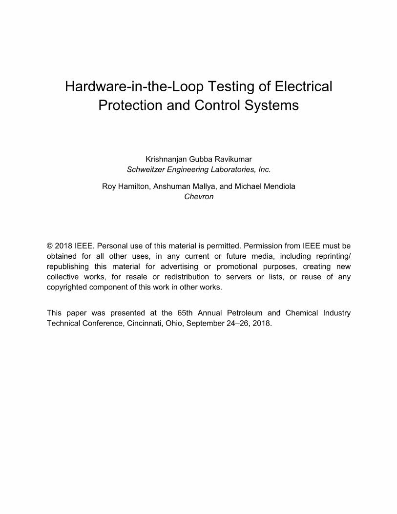
A. Case 1
Case 1 shows the load-acceptance behavior of a Plant 4 gas turbine generator (with IEEE GGOV1 governor model) for three different acceptance values. This test was conducted during the model validation stage for verifying individual generator responses. Fig. 8 shows the plotted machine speed, mechanical power, and bus frequency values. These results were compared to the manufacturer’s expected responses to tune the governor models. Overall, they compared well, and minimal tuning was required to bring them closer.
100
99
98
Fre
que
ncy
(Hz)
100
110
90
80
7050
49.849.649.449.2
49
Time (s)406.67 13.33 26.67 33.330 20
Wper 20 MW
Wper 10 MW
Wper 30 MW
Pmech 10 MW
Pmech 20 MW
Pmech 30 MW
Busfreq 10 MWBusfreq 20 MW
Busfreq 30 MW
99.5
Spe
ed (
%)
Mec
hani
cal
Pow
er (
MW
)
98.5
Fig. 8 Load Acceptance Responses for a Plant 4 Generator
B. Case 2
Case 2 represents a situation where a local generator was tripped while the plant was still connected to the utility. Most of
the load was picked up by the utility, with a 0.14 Hz deviation in system frequency (see Fig. 9). During this test, the utility tie lines reached 95 percent of their power flow capacity and came very close to being decoupled. This test was conducted during the model validation stage for verifying the overall power system dynamic response.
Freq
uenc
y (H
z)Bu
s Vo
ltage
(pu)
50.05
50
49.95
49.9
49.85
1.02
1.01
1
0.99
0.98
0.97
0.96
Main
Plant 4
Plant 3Plant 2
Plant 1
Fig. 9 Loss of Local Generator While Connected to Utility
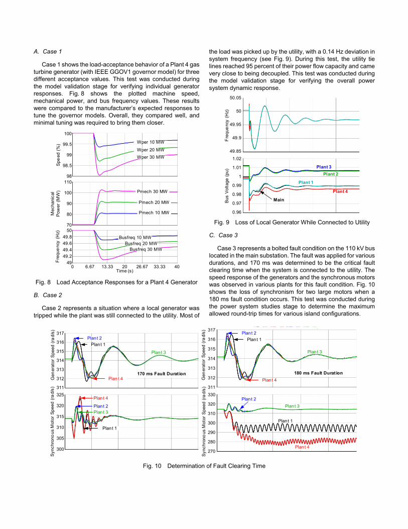
C. Case 3
Case 3 represents a bolted fault condition on the 110 kV bus located in the main substation. The fault was applied for various durations, and 170 ms was determined to be the critical fault clearing time when the system is connected to the utility. The speed response of the generators and the synchronous motors was observed in various plants for this fault condition. Fig. 10 shows the loss of synchronism for two large motors when a 180 ms fault condition occurs. This test was conducted during the power system studies stage to determine the maximum allowed round-trip times for various island configurations.
317
316
315
314
312
311
313
317
316
315
314
312
311
313
325
320
315
310
305
300
330
320
310
300
290
280
270
170 ms Fault Durat ion 180 ms Fault Durat ion
Plant 1
Gen
erat
or S
peed
(ra
d/s)
Gen
erat
or S
peed
(ra
d/s)
Syn
chro
nous
Mot
or S
peed
(ra
d/s)
Syn
chro
nous
Mot
or S
peed
(ra
d/s)
Plant 1
Plant 4
Plant 2
Plant 3
Plant 4
Plant 2Plant 3
Plant 1
Plant 4
Plant 2
Plant 3
Plant 1
Plant 4
Plant 2Plant 3
Fig. 10 Determination of Fault Clearing Time
D. Case 4
Case 4 (see Fig. 11) represents an HIL test where the load-shedding system shed load for the loss of a generator and quickly stabilized the power system during a summer operating case. In this case, all the generators were operating at their full capacity (pre-event) and the plant would have separated at the utility connection if a load-shedding action did not occur. The separation of the plant is undesired in this case because it would create a generation deficit that could collapse the island. This test was conducted during the HIL testing stage to validate the performance and effectiveness of the load-shedding system.
50.011
49.996
49.981
49.967
49.952
49.938
49.9231.02
0.98
0.96
1
0 10 20 30 40 50
Fre
que
ncy
(Hz)
Bus
Vol
tage
(pu
)
Plant 4
Plant 3Plant 2
Plant 1
Main
Time (s)
Fig. 11 Load-Shedding Operation to Preserve System Stability
Overall, the authors performed more than 100 HIL tests to validate control system performance during project development and factory acceptance testing. Some of the key lessons learned from the HIL testing include the following:
1. HIL testing provides a mechanism to understand the power system’s dynamic response to control actions.
2. For optimized load shedding within the plant, compensate the decoupling scheme with IRMs and DRMs. This allows for proper classification of events and appropriate high- or low-speed actions.
3. To obtain a better frequency response during islanded conditions, revise the relay-based underfrequency set points to better coordinate with the centralized frequency-based load shedding.
4. To reduce the inherent risks of generation shedding and runback control, a grouped runback of generators is recommended in addition to an optimal combination of generators for shedding.
5. To prevent inadvertent overloading of a single utility tie line, combine the IRM and DRM set points for the overall utility connection.
6. Use rate-of-change of frequency in addition to the static frequency thresholds when developing underfrequency load-shedding schemes for a reliable backup scheme.
V. CONCLUSIONS
HIL tests play a critical role in testing control systems before they are deployed in the field. Through HIL tests, the performance and effectiveness of PMS controls can be studied for both typical cases and corner cases that cannot be verified in the field. Also HIL testing reduces overall commissioning time and is great for brownfield integration projects where production disruption can be critical. This paper discusses the theory and steps involved in developing a simulation system using a DRTS and actual field controllers. The architecture, applications, and key features are detailed to help describe the implementation. Key takeaways include the following:
1. Protection and control systems should be thoroughly tested and proved before they are deployed in the field. Closed-loop tests allow for true continuous interaction with the power system.
2. To meet HIL testing objectives, proper dynamic models must be developed and validated prior to testing. Also, proper protection and control system set points should be programmed into the model to represent existing field conditions.
3. The simulation system architecture should closely represent the field setup, including the interfacing protocols. This ensures proper consideration of delays and other nonlinearities.
4. Simulation systems can aid operator decision making before field modifications are implemented.
5. HIL testing helps identify vulnerabilities within the power system for better protection.
VI. ACKNOWLEDGEMENT
The authors would like to acknowledge the efforts of Mr. Mahipathi Appanagari and Mr. Tim George Paul for their contributions to the design, development, and testing of the simulation system.
VII. REFERENCES
[1] K. G. Ravikumar, T. Alghamdi, J. Bugshan, S. Manson, and S. K. Raghupathula, “Complete Power Management System for an Industrial Refinery,” proceedings of the 62nd Annual Petroleum and Chemical Industry Technical Conference, Houston, TX, October 2015.
[2] K. Hao, A. R. Khatib, N. Shah, and N. Herbert, “Case Study: Integrating the Power Management System of an Existing Oil Production Field,” proceedings of the 63rd Annual Petroleum and Chemical Industry Technical Conference, Philadelphia, PA, September 2016.
[3] E. R. Hamilton, J. Undrill, P. S. Hamer, and S. Manson, “Considerations for Generation in an Islanded Operation,” proceedings of the 56th Annual Petroleum and Chemical Industry Conference, Anaheim, CA, September 2009.
[4] K. G. Ravikumar, A. Upreti, and A. Nagarajan, “State-of-the-Art Islanding Detection and Decoupling Systems for Utility and Industrial Power Systems,” proceedings of the 69th Annual Georgia Tech Protective Relaying Conference, Atlanta, GA, April 2015.
VIII. VITAE
Krishnanjan Gubba Ravikumar received his M.S.E.E. degree from Mississippi State University and his B.S.E.E. degree from Anna University, India. He is presently working as a senior engineer in the SEL Engineering Services division, focusing on the design, development, and testing of special protection systems. His areas of expertise include real-time modeling and simulation, synchrophasor applications, remedial action schemes, power management systems, and power electronic applications. He has extensive knowledge of power system controls and renewable distributed generation. He is a senior member of the IEEE and a member of the Eta Kappa Nu Honor Society. He can be contacted at [email protected].
Roy Hamilton received his undergraduate degree in electrical engineering from the Georgia Institute of Technology in 1980. He has worked as an electrical design engineer for the Tennessee Valley Authority and as an I&E project engineer for DuPont and Amoco. He also served as an electrical operations engineer for nine years in Saudi Aramco’s Northern Area Producing Department. Currently, he is working as the Electrical Lead for Chevron’s Future Growth Project. He is a member of the IEEE and IEEE IAS. He can be contacted at [email protected].
Anshuman Mallya is a senior electrical power systems engineer with Chevron’s Energy Technology Company. His responsibilities include the design, development, and testing of power management, fast load-shedding, generation control, and closed-loop simulation systems while maintaining the associated Chevron engineering standards. He received his B.S. in electrical engineering in 2001. He is a member of IEEE. He can be contacted at [email protected].
Michael Mendiola received both his bachelor’s and master’s degrees in electrical engineering from California Polytechnic State University, San Luis Obispo, in 2008. He joined Chevron in 2007 and worked in Chevron’s Engineering Technology Company as an electrical engineering power systems specialist based in Houston, Texas. From 2011 to the present, he has been working as a project electrical discipline engineer on a major capital project for Tengizchevroil and is currently based in Farnborough, United Kingdom. He is a member of IEEE. He can be contacted at [email protected].
Previously presented at the 65th Annual Petroleum and Chemical Industry Technical Conference, Cincinnati, Ohio, September 2018.