Page 1
DOI 10.1515/secm-2013-0194 Sci Eng Compos Mater 2013; aop
Zeki K ı ral *
Harmonic response analysis of symmetric laminated composite beams with different boundary conditions Abstract: This study deals with the determination of the
harmonic response of symmetric laminated composite
beams by the finite element method. The structural stiff-
ness of the composite beam is determined by the classi-
cal laminated plate theory. Four different ply orientations,
namely, [0] 2s
, [0/90] s , [45/-45]
s , and [90]
2s are used to exam-
ine the effect of the stacking sequence on the harmonic
response of the beam. Proportional damping is used to
model the structural damping, and the damped harmonic
responses of the composite beams are obtained to show
the effect of the damping on the harmonic response.
The effect of the boundary conditions on the harmonic
response is also investigated. The displacement maps
calculated for varying excitation points are obtained for
different boundary conditions and damping ratios at dif-
ferent vibrational modes. The numerical results presented
in this study show that the magnitudes of the harmonic
response of the composite beam increase as the flexural
rigidity decreases, and the vibration magnitudes reduce
considerably with damping. The vibration patterns cre-
ated for varying excitation and observation locations
change as the damping ratio and excitation frequency
change.
Keywords: finite element method; harmonic response;
laminated composite beam; numerical integration; pro-
portional damping.
*Corresponding author: Zeki K ı ral, Faculty of Engineering,
Department of Mechanical Engineering, Dokuz Eyl ü l University,
35397 T ı naztepe-Buca, İ zmir, Turkey, e-mail: [email protected]
1 Introduction Engineering structures are generally subjected to time
varying excitations. Among them, harmonic excitation is
one of the most encountered loading types in which the
magnitude of the external load varies within a harmonic
envelope. The source of the harmonic excitation in engi-
neering structures is generally an unbalanced rotating
component. The frequency and location of the harmonic
excitation and the eigenfrequencies of the structure are
the main factors that affect the magnitude and the form
of the structural vibration. Determination of the har-
monic response of the lightweight structures in which the
composite members are involved is of great importance
especially at the design stage. Studies related to dynamic
response of the composite structures in the form of beams
and plates generally deal with the calculation of the
natural frequencies of the considered structure using ana-
lytical or numerical techniques. Contribution to the calcu-
lation of harmonic response of the composite structures
constitutes the main motivation of this study.
Because of the importance of the subject, research-
ers have paid attention to the calculation of the dynamic
response of the engineering structures. The studies on the
dynamic response analyses of engineering structures, which
are composed of isotropic or composite materials, have been
focused mainly on the calculation of free vibration frequen-
cies. Calculation of free vibration frequencies is important to
avoid the resonance phenomenon, but it is also important
to know the vibration levels in a broad range of harmonic
excitation frequency. Vaziri and Nayeb-Hashemi presented
the results of the dynamic response of repaired composite
beams subjected to harmonic peeling load [1] . They used the
finite element method to present the discrepancies between
the theoretical and the experimental results.
Rao and Ganesan used the finite element method in
order to study the harmonic response of tapered com-
posite beams [2] . Makhecha et al. studied the transient
dynamics and damping analysis of laminated sandwich
composite plates [3, 4] . Raja et al. [5] presented the free and
forced harmonic vibration control of composite beams by
active stiffening method using piezoelectric patches. They
reported that the active stiffening effect through displace-
ment control is more effective for smaller modes. Sun and
Huang proposed an analytical formulation to perform the
active vibration control of laminated composite beams
equipped with a piezoelectric sensor and actuator layers
under harmonic loading conditions [6] .
K ı ral investigated the harmonic response of a pinned-
pinned laminated composite beam using the finite element
Brought to you by | St. Petersburg State UniversityAuthenticated | 93.180.53.211
Download Date | 12/28/13 3:41 PM
Page 2
2 Z. K ı ral: Harmonic response analysis of symmetric laminated composite beams
method [7] and presented the effect of the damping on the
frequency response of the composite beam with the aid of
proportional damping assumption. Ribeiro [8] studied the
forced vibrations of composite laminated plates by using a
p version, hierarchical finite element including the effects
of rotary inertia, transverse shear, and geometrical non-
linearities. Patel et al. [9] studied the transient response of
anisotropic laminated composite plates by using the finite
element method. Parhi et al. [10] proposed a delamina-
tion model to analyze the dynamic behavior of laminated
composite plates possessing multiple delaminations by
using the finite element method. Bilasse and Oguamanam
[11] presented the forced harmonic response of large-scale
viscoelastic sandwich plates by combining the asymptotic
numerical method and reduction techniques based on the
modal analysis.
The aim of this study is to examine mainly the
harmonic response of a composite beam with differ-
ent boundary conditions, namely, clamped-clamped,
clamped-pinned, pinned-pinned, and clamped-free. The
finite element method is used in association with the
Newmark time integration method, which is a powerful
tool for structural dynamic analysis. In this study, four
different lay-up configurations, namely, [0] 2s
, [0/90] s , [45/-
45] s , and [90]
2s are considered in order to show the effect
of the layup orientation on the frequency response of the
beam. The effect of the location of the harmonic excitation
is also investigated and displacement maps are obtained
for undamped and damped cases. The structural damping
is considered using the proportional damping assump-
tion, and the effect of the damping on the frequency
response of the beam is presented.
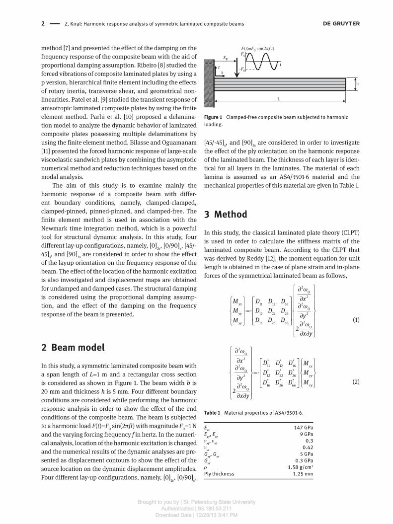
2 Beam model In this study, a symmetric laminated composite beam with
a span length of L = 1 m and a rectangular cross section
is considered as shown in Figure 1 . The beam width b is
20 mm and thickness h is 5 mm. Four different boundary
conditions are considered while performing the harmonic
response analysis in order to show the effect of the end
conditions of the composite beam. The beam is subjected
to a harmonic load F ( t ) = F 0 sin(2 π ft ) with magnitude F
0 = 1 N
and the varying forcing frequency f in hertz. In the numeri-
cal analysis, location of the harmonic excitation is changed
and the numerical results of the dynamic analyses are pre-
sented as displacement contours to show the effect of the
source location on the dynamic displacement amplitudes.
Four different lay-up configurations, namely, [0] 2s
, [0/90] s ,
x z
h
L
F(t)=F0 sin(2πf t) F0XF
-F0
t
Figure 1 Clamped-free composite beam subjected to harmonic
loading.
Table 1 Material properties of AS4/3501-6.
E xx
147 GPa
E yy
, E zz
9 GPa
ν xy
, ν xz
0.3
ν yz
0.42
G xy
, G xz
5 GPa
G yz
0.3 GPa
ρ 1.58 g/cm 3
Ply thickness 1.25 mm
[45/-45] s , and [90]
2s are considered in order to investigate
the effect of the ply orientation on the harmonic response
of the laminated beam. The thickness of each layer is iden-
tical for all layers in the laminates. The material of each
lamina is assumed as an AS4/3501-6 material and the
mechanical properties of this material are given in Table 1 .
3 Method In this study, the classical laminated plate theory (CLPT)
is used in order to calculate the stiffness matrix of the
laminated composite beam. According to the CLPT that
was derived by Reddy [12] , the moment equation for unit
length is obtained in the case of plane strain and in-plane
forces of the symmetrical laminated beam as follows,
2
O
2
211 12 16
O
12 22 26 2
216 26 66O
-
2
xx
yy
xy
xM D D DM D D D
yD D DM
x y
ω
ω
ω
⎧ ⎫∂⎪ ⎪
∂⎧ ⎫ ⎪ ⎪⎡ ⎤⎪ ⎪ ∂⎪ ⎪⎢ ⎥=⎨ ⎬ ⎨ ⎬⎢ ⎥ ∂⎪ ⎪ ⎪ ⎪⎢ ⎥
⎣ ⎦⎩ ⎭ ⎪ ⎪∂⎪ ⎪∂ ∂⎩ ⎭
(1)
2
O
2* * *
11 12 162
* * *O
12 22 262
* * *2 16 26 66
O
-
2
xx
yy
xy
x D D D MD D D M
y MD D D
x y
ω
ω
ω
⎧ ⎫∂⎪ ⎪
∂ ⎧ ⎫⎡ ⎤⎪ ⎪⎪ ⎪∂ ⎢ ⎥⎪ ⎪
=⎨ ⎬ ⎨ ⎬⎢ ⎥∂⎪ ⎪ ⎪ ⎪⎢ ⎥⎣ ⎦⎩ ⎭⎪ ⎪∂
⎪ ⎪∂ ∂⎩ ⎭
(2)
Brought to you by | St. Petersburg State UniversityAuthenticated | 93.180.53.211
Download Date | 12/28/13 3:41 PM
Page 3
Z. K ı ral: Harmonic response analysis of symmetric laminated composite beams 3
where *
ijD denotes the elements of the inverse of D ij . In the
derivation of the laminated beam theory, it is assumed
everywhere in the beam that
M yy
= M xy
= 0 (3)
To complete the theory, it is also assumed that the
laminated beam is long enough to disregard the effects
of the Poisson ratio and shear coupling on the deflection.
Then,
2
*o
112- xxD M
xω∂
=∂
(4)
The following quantities can be used in order to write
Eq. (4) in the familiar form used in the classical Euler-Ber-
noulli beam theory
3 *
11
12, b
xx xxM b M Eh D
= =
(5)
The coordinate system, which is used in deriving the
layer stiffness, is shown in Figure 2 . In this study, vertical
translation ω and rotation θ within a beam element are
used as follows,
2 3 o
o 1 2 3 4( ) , ( )x a a x a x a x x
xω
ω θ∂
= + + + =∂
(6)
Figure 3 shows the elemental length of the beam,
where subscripts 1 and 2 denote the beam ends x = 0 and
x = d , respectively. Then the displacement vector of a beam
finite element is described as
e 1 1 2 2{ } { }Tq ω θ ω θ=
(7)
h/2
h/2 zk+1
z1z2
zk
z
x
Figure 2 Coordinate locations of plies in laminated composite beam.
ω1 ω2
θ2θ1
d
Figure 3 Elemental length of the beam.
The elastic strain energy and kinetic energy of an ele-
mental laminated beam, respectively, are given as follows,
2 22
o o
2
0 0
1 1 and
2 2
d dbxx yy
d dU E I dx T A dx
dtdxω ω
ρ⎛ ⎞ ⎛ ⎞
= =⎜ ⎟ ⎜ ⎟⎝ ⎠⎝ ⎠∫ ∫
(8)
The stiffness [K e ] and mass matrices [M
e ] of an ele-
mental beam are obtained from elastic strain energy and
kinetic energy expressions.
e e e e e e
1 1{ } [ K ] { } , { } [ M ] { }
2 2
T TU q q T q q= = � �
(9)
As the basis of the finite element method, the overall
mass and stiffness matrices are obtained by assembling
the element matrices. The number of elements used in
the finite element vibration analysis is 20. The dynamic
response of the laminated composite beam is calculated
by using the procedure described in the Newmark integra-
tion method, which is widely used in structural dynamics.
By using the overall mass [M], damping [C], and stiffness
[K] matrices for the composite beam, the governing equa-
tions of the system are written in the matrix form as
[ M ] { } [ C ]{ } [ K ] { } { }t t t tq q q F+ + =�� �
(10)
where { } ,tq�� { } ,tq� and { q } t are the nodal acceleration,
velocity, and displacement vectors at time t , respectively.
{ F } t is the external excitation vector including the nodal
excitations at time t and its elements are zero except for
the vertical degree of freedom of the excitation node. For
the case of harmonic excitation applied at a node, the mag-
nitude of the corresponding element of the force vector
is changed with time in a sinusoidal manner. Eq. (10) is
solved for nodal displacement, velocity, and acceleration
by numerical time integration. The integration constants
are defined in the Newmark method as follows [13] ,
0 1 2 3 42
5 6 7
1 1 1, , , 1, 1,
2
2 , ( 1 ), 2
a a a a at tt
ta a t a t
γ γ
β Δ β Δ β ββ Δ
Δ γΔ γ γΔ
β
= = = = − = −
⎛ ⎞ ⎛ ⎞= − = − =⎜ ⎟ ⎜ ⎟⎝ ⎠ ⎝ ⎠
(11)
where Δ t is the time increment used in the numeric analy-
sis. It is well known that the proper selection of the time
increment is very important in the structural dynamic
analysis in order to take into account the effect of the
higher modes in the dynamic response. The time incre-
ment is used as Δ t = T 10
/20, where T 10
is the 10th natural
period of the beam. The integration parameters β and γ are selected as 1/4 and 1/2, respectively, in order to obtain
a stable solution. In the Newmark method, the effective
stiffness matrix can be calculated as
Brought to you by | St. Petersburg State UniversityAuthenticated | 93.180.53.211
Download Date | 12/28/13 3:41 PM
Page 4
4 Z. K ı ral: Harmonic response analysis of symmetric laminated composite beams
[K ef
] = [K] + a 0 [M] + a
1 [C] (12)
The effective load vector F ef
is calculated for each time step
as
ef 0 2 3
1 4 5
{ } { } [ M ] ( { } { } { } )
[ C ] ( { } { } { } )t t t t t
t t t
F F a q a q a qa q a q a qΔ+= + + +
+ + +� ��
� ��
(13)
Then, the nodal displacement, acceleration, and velocity
responses at time t + Δ t can be obtained by using the fol-
lowing equations
{ q } t + Δ t = [K
ef ] -1 { F
ef } (14)
0 2 3{ } ({ } -{ } )- { } - { }t t t t t t tq a q q a q a q
Δ Δ+ +=�� � ��
(15)
6 7{ } { } { } { }t t t t t tq q a q a q
Δ Δ+ += + +� � �� ��
(16)
In this study, the structural damping is modeled as Ray-
leigh damping in which the damping matrix [C] of the
beam is formed by the linear combination of mass and
stiffness matrices as
[C] = c 0 [M] + c
1 [K] (17)
where c 0 is the mass proportional damping coefficient
and c 1 is the stiffness proportional damping coefficient.
Proportional damping assumption easily provides
information about the damped response of the consid-
ered structure, and therefore the Rayleigh damping is
commonly used in structural dynamics. If the damping
ratios ζ m
and ζ n are known for two specific natural frequen-
cies ω m
and ω n , Rayleigh damping coefficients c
0 and c
1 can
be calculated by the solution of the following equation [12] .
0
2 2
1
-2
-1 1-
n mm n m
nn mn m
cc
ω ωω ω ζ
ζω ωω ω
⎡ ⎤⎧ ⎫ ⎧ ⎫⎪ ⎪ ⎪ ⎪⎢ ⎥=⎨ ⎬ ⎨ ⎬⎢ ⎥⎪ ⎪ ⎪ ⎪⎩ ⎩⎭ ⎭⎢ ⎥⎣ ⎦
(18)
In this study, first two fundamental free vibration modes
and the corresponding natural frequencies are considered
to calculate the damping coefficients c 0 and c
1 . The same
damping ratio ζ = 0.02 is used for both vibration modes in
order to calculate the damped response of the composite
beam following the numerical procedure described above.
This damping ratio is compatible with the damping ratios
presented in the literature [14, 15] .
4 Numerical results The dynamic response of the composite beam subjected
to the harmonic loading is calculated for different lay-ups,
Table 2 Comparison of first three natural frequencies obtained from Matlab code and LUSAS.
Natural frequencies (Hz)
f n1 f n2 f n3
Present LUSAS % Dif. a Present LUSAS % Dif. a Present LUSAS % Dif. a
Clamped-clamped
[0] 2s
47.931 48.010 0.164 130.290 132.400 1.593 250.010 260.100 3.879
[0/45] s 46.360 45.920 -0.958 126.020 126.700 0.536 241.820 248.800 2.805
[45/-45] s 16.380 16.260 -0.738 44.526 44.870 0.766 85.438 88.280 3.219
[90] 2s
12.141 11.880 -2.196 33.003 32.770 -0.711 63.327 64.380 1.635
Clamped-pinned
[0] 2s
33.048 33.080 0.097 105.750 107.300 1.444 216.230 224.100 3.511
[0/45] s 31.965 31.640 -1.027 102.290 102.600 0.302 209.150 214.300 2.403
[45/-45] s 11.294 11.140 -1.382 36.140 36.000 -0.389 73.895 75.220 1.761
[90] 2s
8.370 8.185 -2.260 26.787 26.540 -0.930 54.771 55.470 1.260
Pinned-pinned
[0] 2s
21.166 21.180 0.066 83.638 84.720 1.277 184.470 192.900 4.370
[0/45] s 20.472 20.270 -0.996 80.897 80.980 0.102 178.430 182.500 2.230
[45/-45] s 7.233 7.298 0.890 28.582 28.020 -2.005 63.042 63.560 0.815
[90] 2s
5.361 5.239 -2.328 21.185 20.960 -1.073 46.727 47.230 1.065
Clamped-free
[0] 2s
7.573 7.544 -0.384 47.201 47.281 0.169 130.49 132.500 1.517
[0/45] s 7.325 7.213 -1.552 45.654 45.210 -0.982 126.22 126.700 0.378
[45/-45] s 2.588 2.523 -2.576 16.130 15.820 -1.959 44.594 44.350 -0.550
[90] 2s
1.918 1.867 -2.731 11.956 11.700 -2.188 33.053 32.780 -0.832
a Natural frequency value calculated using LUSAS FE program is used as reference value.
Brought to you by | St. Petersburg State UniversityAuthenticated | 93.180.53.211
Download Date | 12/28/13 3:41 PM
Page 5
Z. K ı ral: Harmonic response analysis of symmetric laminated composite beams 5
0 1 2 3-6
0
6
Time (s)
uz(m
m)
0 1 2 3-6
0
6
Time (s)
uz(m
m)
0 1 2 3 4-70
0
70
Time (s)
uz(m
m)
0 1 2 3 4-70
0
70
Time (s)
uz(m
m)
0 1 2 3-350
0
350
Time (s)
uz(m
m)
0 1 2 3-350
0
350
Time (s)
uz(m
m)
A
C
B
D
E F
ζ=0 .0 ζ=0 .02
Figure 4 Midpoint displacement responses of the clamped-clamped composite beam with [90] 2s
lay-up at (A, B) f = 5 Hz, (C, D) 11.5 Hz, and
(E, F) 12.14 Hz when the excitation is applied at the beam midpoint.
-50
-25
0
25
50
0 20 40 60 80 100Excitation frequency (Hz)
20 L
og 1
0(u z)
max
[0]2s [0/45]s[45/-45]s [90]2s
Figure 5 Frequency responses of the pinned-pinned composite
beams calculated for the point x = 0.25 L when the harmonic excita-
tion is applied at x F = 0.25 L , ζ = 0.02.
boundary conditions, damping ratios, and excitation loca-
tions by the numerical integration method. The results of
the numerical analyses are given in this section.
Before the harmonic response analysis, the natural
frequencies of the composite beam for considered lay-up
configurations and boundary conditions are calculated
using the developed Matlab code (The Mathworks Inc.,
Novi, MI, USA). For the comparison purpose, the first
three natural frequencies are also calculated by LUSAS
(LUSAS, Surrey, UK) commercial finite element software.
The results for three natural frequencies are given in
Table 2 . It is seen from the table that there is a good agree-
ment between the numerical results.
-40
-30
-20
-10
0
10
20
30
40
50
0 10 20 30 40 50Excitation frequency (Hz)
20 L
og10
(uz)
max
Clamped-clamped Pinned-pinnedClamped-pinned Clamped-free
Figure 6 Frequency responses of the composite beams with [45/-45]s lay-up calculated for the point x = 0.25 L when the harmonic excitation
is applied at x F = 0.25 L , ζ = 0.02.
Brought to you by | St. Petersburg State UniversityAuthenticated | 93.180.53.211
Download Date | 12/28/13 3:41 PM
Page 6
6 Z. K ı ral: Harmonic response analysis of symmetric laminated composite beams
xresp
(mm)
x F(m
m)
50 200 350 500 650 800 95050
200
350
500
650
800
950
0
0.5
1
1.5
2
2.2
zmax
(mm)A B
C D
E F
xresp
(mm)
x F(m
m)
50 200 350 500 650 800 95050
200
350
500
650
800
950
0.3
0.6
0.9
1.2
1.5
1.8zmax
(mm)
0
xresp
(mm)
x F(m
m)
50 200 350 500 650 800 95050
200
350
500
650
800
950
0.3
0.6
0.9
1.2
1.5
1.8
0
zmax
(mm)
xresp
(mm)
x F(m
m)
50 200 350 500 650 800 95050
200
350
500
650
800
950
0
0.1
0.2
0.3
0.4
0.5
0.6
0.7
zmax
(mm)
xresp
(mm)
x F (
mm
)
50 200 350 500 650 800 95050
200
350
500
650
800
950
0
0.1
0.2
0.3
0.4
0.5
zmax
(mm)
xresp
(mm)
x F (
mm
)
50 200 350 500 650 800 95050
200
350
500
650
800
950
0
0.025
0.05
0.075
0.1
0.125
0.15
zmax
(mm)
Figure 7 Displacement maps of the clamped-clamped composite beam with [45/-45] s lay-up (A) 5 Hz, ζ = 0.0, (B) 5 Hz, ζ = 0.02, (C) 50 Hz,
ζ = 0.0, (D) 50 Hz, ζ = 0.02, (E) 100 Hz, ζ = 0.0, and (F) 100 Hz, ζ = 0.02.
Figure 4 shows the harmonic response of the clamped-
clamped composite beam with [90] 2s
lay-up. Figure 4A and
B shows the undamped and damped harmonic response
of the composite beam at 5 Hz, respectively. As seen from
Figure 4B, damping removes the transient effects in short
time duration and the beam vibrates harmonically at the
excitation frequency. Figure 4C and D shows the harmonic
response at 11.5 Hz. This frequency value is very close to
Brought to you by | St. Petersburg State UniversityAuthenticated | 93.180.53.211
Download Date | 12/28/13 3:41 PM
Page 7
Z. K ı ral: Harmonic response analysis of symmetric laminated composite beams 7
xresp
(mm)
x F (
mm
)
50 200 350 500 650 800 95050
200
350
500
650
800
950
0
1
2
3
4
5A z
max (mm)
xresp
(mm)
x F (
mm
)
50 200 350 500 650 800 95050
200
350
500
650
800
950
0.5
1
1.5
2
2.5
3
3.6
0
B zmax
(mm)
xresp
(mm)
x F (
mm
)
50 200 350 500 650 800 95050
200
350
500
650
800
950
0
0.2
0.4
0.6
0.8
1C z
max(mm)
xresp
(mm)
x F (
mm
)
50 200 350 500 650 800 95050
200
350
500
650
800
950
0
0.05
0.1
0.15
0.2
0.25
0.3
0.35D z
max (mm)
xresp
(mm)
x F (
mm
)
50 200 350 500 650 800 95050
200
350
500
650
800
950
0
0.1
0.2
0.3
0.4
0.5E z
max(mm)
xresp
(mm)
x F (
mm
)
50 200 350 500 650 800 95050
200
350
500
650
800
950
0
0.02
0.04
0.06
0.08
0.1F z
max(mm)
Figure 8 Displacement maps of the clamped-pinned composite beam with [45/-45] s lay-up (A) 5 Hz, ζ = 0.0, (B) 5 Hz, ζ = 0.02, (C) 50 Hz,
ζ = 0.0, (D) 50 Hz, ζ = 0.02, (E) 100 Hz, ζ = 0.0, and (F) 100 Hz, ζ = 0.02.
the first natural frequency of the composite beam, and
the beating phenomenon in which the dynamic response
builds up and then ceases down continuously within a
harmonic envelope having the frequency f n - f
exc , occurs
as seen in Figure 4C. Moreover, it is seen from Figure 4D
that the beating phenomenon cannot be seen clearly after
introducing damping but the magnitude of the dynamic
response is still large. Figure 4E and 4F illustrates the
Brought to you by | St. Petersburg State UniversityAuthenticated | 93.180.53.211
Download Date | 12/28/13 3:41 PM
Page 8
8 Z. K ı ral: Harmonic response analysis of symmetric laminated composite beams
xresp
(mm)
x F (
mm
)
50 200 350 500 650 800 95050
200
350
500
650
800
950
0
5
10
15
20A z
max(mm)
xresp
(mm)
x F (
mm
)
50 200 350 500 650 800 95050
200
350
500
650
800
950
0
2
4
6
8
10
12B z
max(mm)
xresp
(mm)
x F (
mm
)
50 200 350 500 650 800 95050
200
350
500
650
800
950
0
0.2
0.4
0.6
0.8
1
1.2C z
max(mm)
xresp
(mm)
x F (
mm
)
50 200 350 500 650 800 95050
200
350
500
650
800
950
0
0.05
0.1
0.15
0.2
0.25
0.30.32
D zmax
(mm)
xresp
(mm)
x F (
mm
)
50 200 350 500 650 800 95050
200
350
500
650
800
950
0
0.1
0.2
0.3
0.4
0.5
0.6
0.70.75
E zmax
(mm)
xresp
(mm)
x F (
mm
)
50 200 350 500 650 800 95050
200
350
500
650
800
950
0
0.03
0.06
0.09
0.12
0.15F z
max(mm)
Figure 9 Displacement maps of the pinned-pinned composite beam with [45/-45] s lay-up (A) 5 Hz, ζ = 0.0, (B) 5 Hz, ζ = 0.02, (C) 50 Hz, ζ = 0.0,
(D) 50 Hz, ζ = 0.02, (E) 100 Hz, ζ = 0.0, and (F) 100 Hz, ζ = 0.02.
midpoint dynamic displacements at the resonance condi-
tion. The magnitude of the dynamic response gets larger
as time passes for the undamped case as expected, and
the dynamic response reaches a steady-state value for
damped case. The damping reduces the midpoint dynamic
displacements considerably at resonance.
Figure 5 shows the displacement frequency response
of the pinned-pinned composite beam with different stack-
ing sequences. Displacement responses are calculated for
the beam point located at x = 0.25 L in order to show two
or more resonance frequencies in the frequency response.
Three resonance frequencies for [45/-45] s and [90]
2s
lay-ups and two resonance frequencies for [0/45] s and
[0] 2s
lay-up configurations can be seen in this figure. The
anti-resonances for the identical excitation and observa-
tion point are also seen in this figure. As seen from the
figure, [90] 2s
lay-up has smaller resonance frequencies
and, consequently, larger resonance displacements due to
Brought to you by | St. Petersburg State UniversityAuthenticated | 93.180.53.211
Download Date | 12/28/13 3:41 PM
Page 9
Z. K ı ral: Harmonic response analysis of symmetric laminated composite beams 9
xresp
(mm)
x F (
mm
)
50 300 550 800 100050
300
550
800
1000
0
20
40
60
80
100A Bz
max(mm)
xresp
(mm)
x F (
mm
)
50 300 550 800 100050
300
550
800
1000
0
5
10
15
20
25
30
35
zmax
(mm)
xresp
(mm)
x F (
mm
)
50 300 550 800 100050
300
550
800
1000
0
2
4
6
8
10
12C z
max(mm)
xresp
(mm)
x F (
mm
)
50 300 550 800 100050
300
550
800
1000
0
0.2
0.4
0.6
0.8
1
1.2D z
max(mm)
xresp
(mm)
x F (
mm
)
50 300 550 800 100050
300
550
800
1000
0
1
2
3
4
5
6
7
8
9E z
max(mm)
xresp
(mm)
x F (
mm
)
50 300 550 800 100050
300
550
800
1000
0
0.2
0.4
0.6
0.8
1
1.2
1.4
1.6F z
max (mm)
xresp
(mm)
x F (
mm
)
50 300 550 800 100050
300
550
800
1000
0
0.5
1
1.5
2
2.5
3
3.5G z
max(mm)
xresp
(mm)
x F (
mm
)
50 300 550 800 100050
300
550
800
1000
0
0.05
0.1
0.15
0.2
0.25
0.3
0.36H z
max (mm)
Figure 10 Displacement maps of the clamped-free composite beam with [45/-45] s lay-up (A) 5 Hz, ζ = 0.0, (B) 5 Hz, ζ = 0.02, (C) 30 Hz, ζ = 0.0,
(D) 30 Hz, ζ = 0.02, (E) 50 Hz, ζ = 0.0, (F) 50 Hz, ζ = 0.02, (G) 100 Hz, ζ = 0.0, and (H) 100 Hz, ζ = 0.02.
Brought to you by | St. Petersburg State UniversityAuthenticated | 93.180.53.211
Download Date | 12/28/13 3:41 PM
Page 10
10 Z. K ı ral: Harmonic response analysis of symmetric laminated composite beams
its small bending rigidity. The [0] 2s
lay-up provides larger
flexural rigidity and, consequently, larger natural fre-
quencies. For this lay-up, the magnitudes of the harmonic
responses are smaller than those obtained for other lay-up
configurations.
Figure 6 shows the effect of the boundary condition
on the frequency response of the composite beam. The
frequency responses of the composite beam with [45/-45] s
lay-up are obtained for the point located at 0.25 L while
the harmonic excitation is applied at x F = 0.25 L . As seen
from the figure, the clamped-free beam has the smallest
first natural frequency due to its small bending rigidity.
However, clamped-clamped beam has the largest first
natural frequency reflecting its high bending rigidity.
The changes in the vibration displacement magnitudes
due to the varying end conditions are clearly seen in this
figure.
The displacement map is a 2D graph showing the dis-
placement levels for different excitation ( x F ) and obser-
vation points ( x resp
) constructed at a specific excitation
frequency. In this study, displacement maps of the com-
posite beam with [45/-45] s lay-up are plotted for four dif-
ferent boundary conditions for considering undamped
and damped cases. The displacement maps are plotted
using 50-mm increment for both excitation and response
points. These displacement maps can be used to find a
suitable location insensitive to structural vibration in
the component placement procedure. These maps have
comprehensive information about the vibration levels
recorded at different observation points for varying exci-
tation points.
The displacement maps given in Figures 7 – 10 have
been plotted to cover the forced vibrations up to 100 Hz.
Figure 7A – F shows the displacement maps of the
clamped-clamped composite beam for 5, 50, and 100 Hz.
Figure 7A, C, and E shows the displacement values for
the undamped case. As shown in these figures, distribu-
tion of the vibration displacement directly reflects the
related mode shape of the composite beam. In Figure 7A,
displacement values get larger when the excitation point
gets closer to the middle of the beam at 5 Hz. This result
is compatible with the first mode shape of the beam.
The same results are valid for the excitation frequencies
50 Hz (Figure 7C) and 100 Hz (Figure 7E). The symmetry
in the displacement maps is due to the boundary condi-
tion. The displacement magnitudes reduce as the excita-
tion frequency increases. Figure 7B, D, and F shows the
displacement maps for the damped case. Two percent
damping ratio is used to show the effect of the damping
on the displacement distribution. The relation between
the excitation-observation points remains the same but
the displacement magnitudes reduce considerably when
damping is introduced.
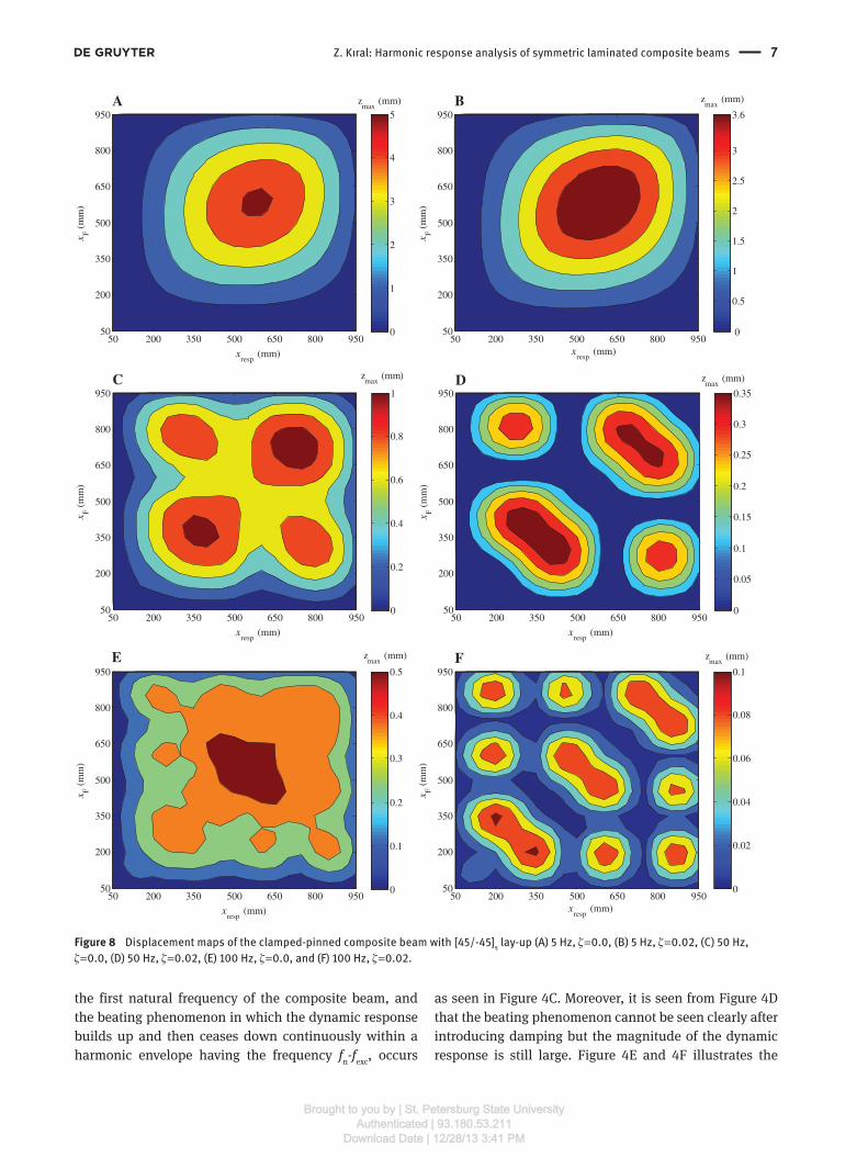
Figure 8A – F shows the displacement maps of the
clamped-pinned composite beam with [45/-45] s lay-up.
This boundary condition is asymmetric, and it is expected
that the displacement distribution has an asymmetric
form. For the clamped-pinned boundary condition, the
displacement values increase when the excitation point is
slightly close to the pinned end of the beam (Figure 8A, C,
and F). The displacement values reduce considerably with
the damping.
Figure 9A – F shows the displacement maps of the
pinned-pinned composite beam with [45/-45] s lay-up.
Similar to the clamped-clamped beam, displacement
values increase as the excitation location moves to the
middle of the beam. Symmetry in the displacement distri-
bution also remains the same for three different excitation
frequencies (Figure 9A, C, and F), and damping reduces
the vibration displacements considerably especially at
higher frequencies (Figure 9B, D, and E).
Figure 10A – H show the displacement maps of the
clamped-free composite beam with [45/-45] s lay-up. This
boundary condition is also asymmetric and the displace-
ment distribution also has an asymmetric form. This
boundary condition has the smallest bending rigidity and
four natural frequencies exist in the 0 – 100 Hz frequency
range. Thus, four different displacement maps at 5, 30, 50,
and 100 Hz are drawn to give the change in the displace-
ment pattern. Similar to the clamped-pinned boundary
condition, the displacement values increase as the excita-
tion point moves to the free end of the beam (Figure 10A,
C, F, and H). As observed for the other boundary condi-
tions, the displacement values reduce considerably with
the damping.
5 Conclusions Determination of the vibration response of the engineer-
ing structures for harmonic excitations is an important
step in structural design. Numerical methods are widely
used for this purpose. The displacement maps of a sym-
metric laminated composite beam having different ply
orientations and boundary conditions are investigated
in this study. The effect of the damping on the frequency
response of the symmetric laminated composite beam
is presented. Stacking sequence and boundary condi-
tion has a decisive effect on the free and forced vibration
characteristics of the symmetric laminated composite
beams. Damping ratio reduces the vibration displacement
Brought to you by | St. Petersburg State UniversityAuthenticated | 93.180.53.211
Download Date | 12/28/13 3:41 PM
Page 11
Z. K ı ral: Harmonic response analysis of symmetric laminated composite beams 11
magnitudes in the harmonic excitation case. The rate of
the reduction is greater for higher vibration modes. In
the case of harmonic excitation, displacement maps can
be obtained using the numerical procedure described in
this study and they can be used in the structural design
of engineering structures, which work under harmonic
excitations.
Received August 16 , 2013 ; accepted September 29 , 2013
References [1] Vaziri A, Nayeb-Hashemi H. Int. J. Adhes. Adhes. 2006, 26,
314 – 324.
[2] Rao SR, Ganesan N. J. Sound Vib. 1997, 200, 452 – 466.
[3] Makhecha DP, Patel BP, Ganapathi M. J. Reinf. Plast. Compos. 2001, 20, 1524 – 1545.
[4] Makhecha DP, Ganapathi M, Patel BP. J. Reinf. Plast. Compos. 2002, 21, 559 – 575.
[5] Raja S, Sinha PK, Prathap G. J. Reinf. Plast. Compos. 2003, 22,
1101 – 1121.
[6] Sun B, Huang D. Compos. Struct. 2001 , 53, 437 – 447.
[7] K ı ral Z. Adv. Compos. Lett. 2009, 18, 163 – 172.
[8] Ribeiro P. Compos. Sci. Technol . 2006, 66, 1844 – 1856.
[9] Patel BP, Gupta SS, Joshi M, Ganapathi M. J. Reinf. Plast. Compos. 2005, 24, 795 – 821.
[10] Parhi PK, Bhattacharyya SK, Sinha PK. J. Reinf. Plast. Compos. 2000, 19, 863 – 882.
[11] Bilasse M, Oguamanam DCD. Compos. Struct. 2013, 105, 311 – 318.
[12] Reddy JN. Mechanics of Laminated Composite Plates and Shells: Theory and Analysis , CRC Press: New York, 1997.
[13] Clough RW, Penzien J. Dynamics of Structures , McGraw-Hill:
New York, 1993.
[14] Berthelot JM, Sefrani Y. Compos. Struct. 2007, 79, 423 – 431.
[15] Berthelot JM, Assarar M, Sefrani Y, El Mahi A. Compos. Struct. 2008, 85, 189 – 204.
Brought to you by | St. Petersburg State UniversityAuthenticated | 93.180.53.211
Download Date | 12/28/13 3:41 PM