HARMONIC STATE ESTIMATION - Shodhgangashodhganga.inflibnet.ac.in/bitstream/10603/8430/16/16_chapter...

40

CHAPTER 4

HARMONIC STATE ESTIMATION

4.1 Introduction

In an interconnected system various loads generate harmonics which spread in the

network and to other loads. It is important to estimate the location of loads and

corresponding buses which generate harmonics. ICA is one of the techniques of

estimation. In Section 3.8, it is mentioned that the four time structured ICA

algorithms to be discussed in this work are FICA, EFICA, EBM and JADE. A FICA

variant algorithm FIWAS is also used to mimic the behaviour of JADE for harmonic

voltage estimation. It is found that for steady state models, the various ICA algorithms

show varying levels of accuracy for the different harmonic frequencies. The best ICA

algorithm based on steady state performance is chosen and it is processed by a

Kalman Filter which functions as an optimal state estimator. The harmonic currents/

voltages are estimated on a simple four bus model and tested on a laboratory four bus

model. The harmonic estimation of voltages and currents are carried out on an IEEE

14 bus system also. In addition to the theoretical simulation, the four bus system is

wired in the laboratory and the harmonic current estimation is carried out on that

system.

4.2 Modelling of Power System Components

The increased use of non-linear loads results in harmonics generation and propagation.

The harmonics generation and its propagation are easy to analyse in a single load circuit.

However, the analysis of harmonics in the form of source estimation and propagation in

interconnected power system requires an in depth study. The main focus for such a study

involves the behavioural study of the various power system components in the presence

of harmonics and measurement of harmonics at selected locations. Generally, the various

power system components are modelled in the following manner by equivalent

impedances as below [73]:

(i) Passive Elements: The impedance of passive elements like resistors,

capacitors and inductors has the following relations with harmonic frequency

‗h‘. The following characteristics are observed by these elements:

41

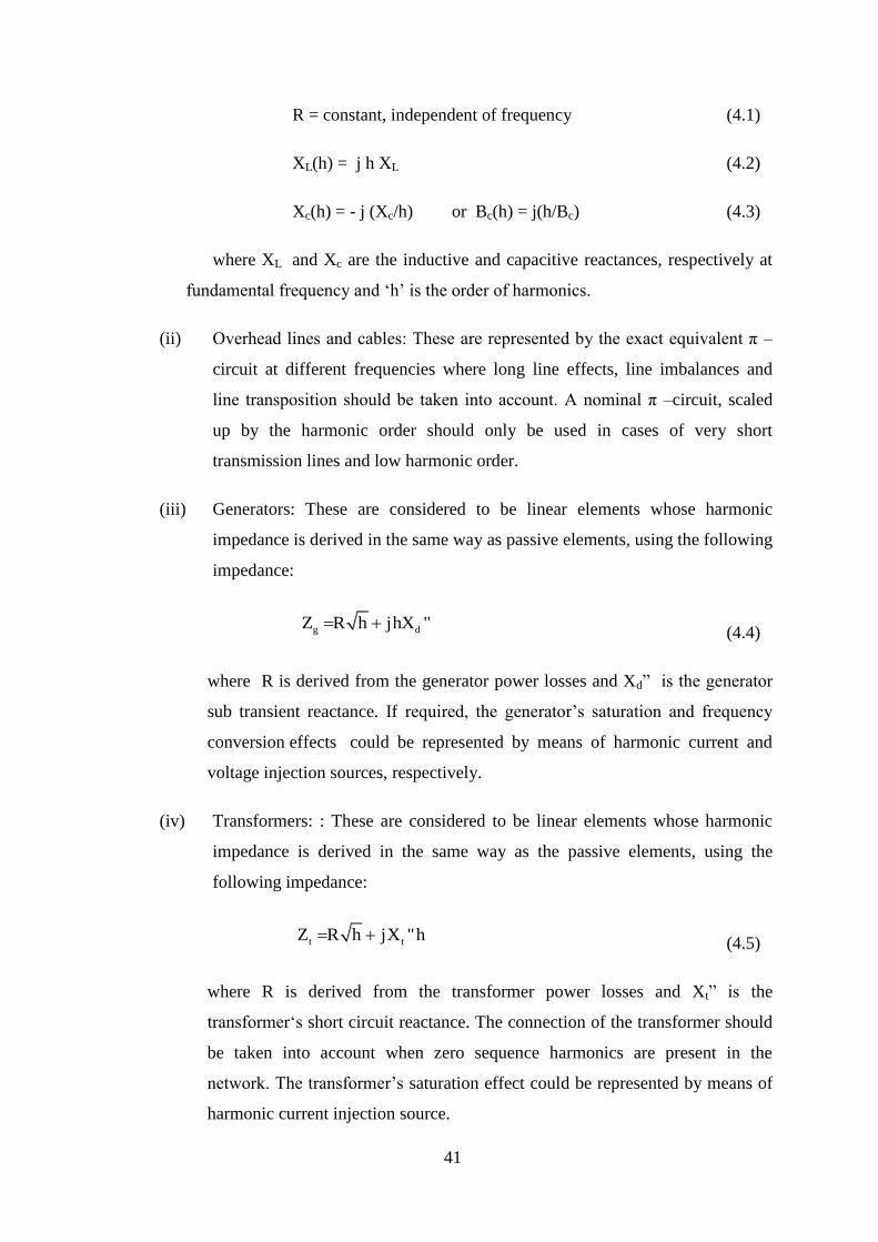
R = constant, independent of frequency (4.1)

XL(h) = j h XL (4.2)

Xc(h) = - j (Xc/h) or Bc(h) = j(h/Bc) (4.3)

where XL and Xc are the inductive and capacitive reactances, respectively at

fundamental frequency and ‗h‘ is the order of harmonics.

(ii) Overhead lines and cables: These are represented by the exact equivalent π –

circuit at different frequencies where long line effects, line imbalances and

line transposition should be taken into account. A nominal π –circuit, scaled

up by the harmonic order should only be used in cases of very short

transmission lines and low harmonic order.

(iii) Generators: These are considered to be linear elements whose harmonic

impedance is derived in the same way as passive elements, using the following

impedance:

(4.4)

where R is derived from the generator power losses and Xd‖ is the generator

sub transient reactance. If required, the generator‘s saturation and frequency

conversion effects could be represented by means of harmonic current and

voltage injection sources, respectively.

(iv) Transformers: : These are considered to be linear elements whose harmonic

impedance is derived in the same way as the passive elements, using the

following impedance:

(4.5)

where R is derived from the transformer power losses and Xt‖ is the

transformer‗s short circuit reactance. The connection of the transformer should

be taken into account when zero sequence harmonics are present in the

network. The transformer‘s saturation effect could be represented by means of

harmonic current injection source.

g dZ R h jhX "

t tZ R h jX "h

42

(v) Capacitor banks: These are considered to be passive elements, where:

(4.6)

VLL is the RMS line voltage in kV and Q 3ϕ is the three –phase reactive power

in MVAR.

(vi) Linear loads: These may be represented by three different models given by the

CIGRE Working Group[74]:

(a) Parallel R-XL equivalent:

Figure 4.1 Parallel R-XL equivalent

where and (4.7)

(b) Parallel R-XL equivalent , where

and (4.8)

where k = 0.1h +0.9

(c) Parallel R-XL in series with XS , where

Figure 4.2 Parallel R-XL in series with Xs equivalent

2

LLc

3

VX (h)

hQ

R XL R

XL(h

)

ih

+

-

2

LL

3

VR

P

2

LLL

3

hVX (h) j

Q

2

LL

3

VR

kP

2

LLL

3

hVX (h) j

kQ

R

XL

Xs

R

hXL

hXs

ih

+

-

2

LL

3

VR

P

43

and (4.9)

The linear loads are modelled in this work using (c).

(vii) Non-linear loads: These are represented by either a harmonic current injection

source or by a harmonic voltage source. Harmonic current injection sources

are used to represent the harmonic contributions of static VAR compensators

(SVCs), induction arc furnaces, rectifiers and electronic appliances. Harmonic

voltage sources are arc furnaces and pulse width modulation (PWM)

converters.

(viii) Transmission Elements: The transmission elements and linear loads are

represented by impedances, at each harmonic h, with which the admittance

matrix Yh of the system is built. The relevant harmonic current and voltage

sources Ih and Vh are injected into the partially inverted nodal admittance

matrix and the remaining nodal harmonic voltages and currents are obtained.

Some of the assumptions made for such a modelling are:

The Power System is balanced and symmetrical.

All the component values are in p.u.

4.3 Harmonic Injecting Sources

The harmonic injection could be due to current sources like Static Var Compensators

(SVCs), High Voltage Direct Current Transmisssion (HVDC) or Asynchronous Speed

Drives (ASDs) or due to voltage sources like Electric Arc Furnace (EAF), PWM

Converters or series compensators.

4.3.1 Harmonic Current Sources

The three main harmonic current injecting sources used in this work are the SVCs,

HVDC and the ASDs.

L

3

3

hRX (h) j

Q6.7 0.74

P

SX (h) j0.073hR

44

SVC is a shunt connected static Static Var Generator/load whose output is adjusted to

exchange capacitive or inductive current so as to maintain or control specific power

system variable. Typically, the power system control variable is the terminal bus voltage.

There are two popular configurations of SVC. One is a fixed capacitor (FC) and thyristor

controlled reactor (TCR) configuration and the other one is a thyristor switched capacitor

(TSC) and TCR configuration. In this work, the first configuration is used to model [60]

the harmonic current injection. The basic harmonic spectra for an SVC are given in

Figure 4.3.

Figure 4.3 Harmonic Spectra of a SVC

A basic HVDC line consists of a three phase supply on either side of the rectifier and an

inverter, both of which are coupled to a D.C. line. This model is derived from [61]. The

basic harmonic spectrum for an HVDC is given in Figure 4.4.

Figure 4.4 Harmonic Spectra of a HVDC

45

AC Adjustable Speed Drives (ASDs) can be thought of as electrical control devices that

change the operating speed of a motor. ASDs are able to vary the operating speed of the

motor by changing the electrical frequency input to the motor. The speed variation is

affected by a converter, inverter and a regulator which work to vary the motor speed. The

ASD model is derived from [62] and the harmonic spectra of an ASD are given in Figure

4.5.

Figure 4.5 Harmonic Spectra of an ASD

4.3.2 Harmonic Voltage Sources

The two main harmonic voltage sources considered in this work are a PWM inverter and

an arc furnace.

In a PWM inverter, the inverter output has to be sinusoidal with both magnitude and

frequency being controllable. To obtain a sinusoidal output voltage at a desired

frequency, a sinusoidal control signal at the desired frequency is compared with a

triangular waveform. The switching frequency of the inverter is based on the frequency of

the triangular waveform and is normally kept constant along with its amplitude vtri. The

triangular waveform vtri operates at a frequency fs which decide the frequency with which

the inverter switches are switched. The control signal vc is used to modulate the switch

duty ratio and has a frequency f1 which is the desired fundamental frequency of the

inverter output. The amplitude modulation ratio is given by ma = vc/vtri. The frequency

modulation ratio is defined as mf = fs/f1. An over modulation (ma>1) scheme is used in

PWM [63], so that the amplitude of the fundamental frequency component in the output

voltage is increased to a value greater than 1. This causes more harmonics to appear in the

voltage. It is this case which is implemented in the work.

46

An electric arc furnace used in steel production is a highly non linear load. It operates

both on a.c. and on d.c. The operating cycle consists of a melting stage and numerous

refining stages. The abnormal behaviour of the arc furnace is due to the random

movement of the melting material which causes the even harmonics also to exist. The

refining stage is accompanied by a large arcing operation. Thus, the arc furnace becomes

a highly varying load which pollutes the entire system. Though, several papers on arc

furnace modelling are available, the harmonic voltage profile in terms of the fundamental

voltage during the melting and refining stage is given in [64]. This information is utilized

to create a random profile for the a.c operated arc furnace. The third and fifth harmonics

are dominant during both the stages.

4.4 ICA Algorithms

Out of the several ICA algorithms, the time structured ICA algorithms used for harmonic

estimation are Fast ICA (FICA) [65, 66], Efficient Variant Fast ICA (EFICA) [67, 68],

Entropy Bound Minimisation (EBM) [69, 70] and Joint Approximate Diagonalisation of

Eigen Matrices (JADE) ICA [71].

4.4.1 FastICA

FastICA is based on maximisation of non-gaussianity. It converges faster and hence the

name FastICA. The learning rule of the algorithm unlike other information –theoretic

models does not require a learning parameter and hence is simpler to design. To prevent

various units from converging at the same maxima, the outputs are decorrelated after each

iteration using Gram-Scmidt like decorrelation. After estimating w1,.....wp, one unit fixed

point algorithm for wp+1 is run and after every iteration the projections of previous

estimated p vectors are subtracted from wp+1 which is normalised as in step five and six.

Algorithm for Complex Fast ICA:

1. Prewhiten and decorrelate the observed vector X.

2. Choose N, the number of independent components and set p=1.

3. Select a random vector wp.

47

4. Set

(4.10)

5. Orthogonalise wp via

(4.11)

6. Normalise wp by:

(4.12)

7. If , = repeat from step2

8. Let p = p+1 , if p ≤ N , iterate from step 2.

4.4.2 EFICA: EFICA an extension of FastICA is more efficient in the presence of finite

data samples. With finite data samples, WA≠ I for FICA, which is due to the variance of

the samples. This is compensated in EFICA by restoring to three simple steps. The

weight W from FICA is taken as the preliminary estimate. Next, based on the numerical

value of fourth order moment, an adaptive choice of nonlinearity function is made.

Finally, a final tuning is carried out using the non- linearities and the parameter cpl. The

various steps of the EFICA algorithm are described in the next section.

Algorithm for EFICA:

1. Prewhiten and decorrelate the observed vector X.

2. For the observed data X, this yields

1/2

eZ C X X (4.13)

where C is the covariance matrix of the sample

and is the sample mean.

3. The fast ICA is applied using the non linear function tanh and

estimates are obtained.

4. Reliable estimates are obtained using saddle points.

2 2 2 2w { ( )* ( )} { '( )}H H H H H

p E x w x g w x E g w x w x g w x w

1

w w (w w )wp

H

p p j j p

j

ww

w

new pp

p

w wnew

p p w p w new

p

X

w p

48

5. Define

new T new

p e pv Z w (4.14)

6. The fourth moment of pth

source signal is computed as:

(4.15)

7. To eliminate the residual error of the algorithm, non linear functions are

assigned according to the range of

(4.16)

8. The weights are got from step 3 and a constant k is calculated:

(4.17)

If k> 0.95 , the one unit fast ICA is iterated. Otherwise is retained

with non-linear function value chosen as tanh.

9. If is the result after the convergence of the one unit

algorithm, a tuning step is necessary as given in step 10 and 11.

10. For tuning, five specific parameters based on non linear function and its

derivatives are formulated:

(4.18)

Based on these parameters, calculate

4

4

1N pp

vm

N

1 4

1

4

14

4

exp 3

( ) ( ). min 1.8 3

( ). 1.8

p

p

p p

p

x x for m

g x sign x x for m

sign x x for m

sym

pw

symT

p pk w w

sym

pw

1[ ,...... ]T

dW w w

2

2

/

1 ' /

1 /

T

pp p p p p p

T

Np p p p p p

T

Np p p

v g v N

g v N

g v N

49

(4.19)

11. The new weights are obtained from as

(4.20)

12. The value of is redefined as:

(4.21)

13. Thus, the demixing matrix is:

(4.22)

4.4.3 EBM

The ICA-EBM algorithm uses a line search procedure which utilises the updates that

constrain the demixing matrix to be orthogonal. For ICA, in order to separate ‗N‘ signals

the mutual information among ‗N‘ random variables yn , n=1,2......N.

(4.23)

where is the entropy of the nth

separated source and H(x) the entropy of

observations which is a constant with respect to ‗x‘.

To measure entropy, the expression for each measuring function E [G(x)] is evaluated

over T observed samples and each expectation leads to an upper bound estimate of H(x)

as

2

1

l

l

p

ppl l

for l pc

for l p

plc

1

1/2

p

p

W ,....... W

W W W W

W

p p pd

old Tp p p

Tnew old

pk

diag c c

w

new

pv

new T new

p pv Z w

Wnew

1W ,.........new new new

dw w

1 2 NI(y ;y ;........y )

N

1 2 N n

n 1

I(y ;y ;........y ) H(y ) log det( ) H(x)

W

nH(y )

50

(4.24)

Minimise with respect to each of row vectors keeping wm,

m=1,2,......n-1,n+1,....N as constant.

Define the upper bound estimator H(x) as :

(4.25)

where is a quantity independent of and is the penalty function. The

gradient of this expression is formulated in [69].

Using the gradient expression obtain the steepest descent direction

(4.26)

where ,

is the gradient of equation 4.25. The normalised

projected gradient is orthogonal to the previous wn and points in the steepest ascent

direction. Thus, the line search algorithm is obtained as:

(4.27)

where µ> 0 is the step length. is computed using equation 4.26. The ICA-EBM

algorithm repeats the line search given in equation 4.27 over different rows of W until

convergence.

bound

kH(x) H (x)

1 2 NI(y ;y ;........y )

J ( ) H(y ) log C Tw h wn nn n n

1C wn

Th w

n n

J ( )( )

+

n n

wu P w

w

n nn

n

+

nn +

n

uu

u

( ) T

nP w I w w

n n n

J ( )

w

w

n n

n

nu

+

n n nw w u

[new] +

nn +

n

ww

w

nu

51

After each row vector in the demixing matrix W has been updated once, a

symmetric decorrelation procedure is performed to keep the demixing matrix

orthogonal, i.e. we use

(4.28)

Thus, this entropy uses the tightest maximum entropy bound for implementing ICA

algorithm.

4.4.4 JADE ICA

JADE ICA is rooted in the joint diagonalization of cumulant matrices. This algorithm

utilises the second and fourth order cumulants for source separation. More details of the

algorithm are found in [71].The various steps of the algorithm as proposed by Jean

Cardoso are briefly given:

1. Prewhiten and decorrelate the sensor readings x.

2. Determine the maximal set of cumulant matrices for x.

3. Estimate an orthogonal matrix R such that it minimizes the contrast

function.

4. Compute the demixing matrix as

A=R-1

* P (4.29)

5. Analyse the independent sources

S=A-1

* x . (4.30)

JADE ICA is normally very accurate and its performance is very close to that of the

actual value.

Using these four algorithms, current and voltage harmonics are estimated in an

interconnected power system using ICA.

1/2

T

W WW W[new]

52

4.4.5 FIWAS

An integration of FICA and WASOBI results in FIWAS. FICA algorithm is explained in

detail in [65, 66]. Weighted adjustment Second Order Blind identification(WASOBI)

employs proper weighting of several time - lagged estimation correlation matrices [72]

and is an enhanced version of Second Order Blind Identification(SOBI).The observed

signals are processed by FICA and then by WASOBI. Such a signal is able to extract the

source signal at all harmonic frequencies irrespective of its amplitude and source

distributions.

4.5 Harmonic Current Estimation

The comparison of ICA algorithms are done on the simulated systems (i) Four Bus

Model (ii) IEEE 14 Bus Model for current estimation . This is followed by verification on

a four bus laboratory model.

4.5.1 Four Bus Model

The four bus test system comprises of two generators, two linear loads, two non linear

loads and four transmission lines linking the four buses. The four bus model is a modified

model given in [73] and its transmission line parameters are obtained from the laboratory

model. The four bus model employed for harmonic current estimation is shown in Figure

4.6.

Figure 4.6 Four Bus Test System

The transmission line parameters used for simulation are obtained from the laboratory

model and are specified in Table 4.1.

G

G

Bus 1Bus 2

Bus 3

Bus 4

L3

L2

Ih

Ih

SVC

HVDC

53

Table 4.1 Transmission Line Parameters for the Laboratory Model

The harmonic current injected into the system is represented by harmonic current

source, one each at buses two and three, whose modelling is given for HVDC [61] and

for SVC [60] and is explained in section 4.3.1.

4.5.1.1 Generation of Data

The four bus test system is to be modelled with the power system components like

transmission lines, linear loads and the current sources. This is done in order that data is

observed and the ICA analysis is applied. The methodology employed for the generation

of observation data (harmonic voltage) is as follows:

1. The linear loads and the other power system components of the four bus

system are modelled as in [73]. The harmonic sources are modelled as

current sources SVC and HVDC. Thus the admittance of the test system is

formulated for a specific harmonic frequency (h = 5).

2. The harmonic current of HVDC and SVC at buses 2 and 3 are

computed at this frequency while the harmonic current values at the

Bus R() XL()

1 – 2 0.116 jh0.7620

2 – 3 0.216 jh1.5039

3 - 4 0.332 jh2.2660

4 – 1 0.1302 jh0.8399

54

remaining buses are taken as zero and a single harmonic voltage data is

generated for the system at h=5.

3. Once the modelling of the power system components and the profiles of

the loads at different frequencies ‗h‘ is fixed, the random profile for the

source is modelled as Poisson distribution to obtain 1440 samples(i.e. 1

sample per minute) on a specific day and the various ICA algorithms are

applied.

4. Using this profile, the harmonic current data is generated at buses 2 and 3

for 1440 readings. Substituting these readings for Ibh and Zh (inverse of

admittance of the test system) in the equation (3.34) defined as:

Vbh=ZhIbh, 1440 values for Vbh are obtained at h = 5.

5. Steps (1) to (4) are repeated for h = 7, 11, 13 and 17 .The corresponding

Vbh data generated are defined as the harmonic voltage sensor readings.

In step (3) the observation data is generated using Poisson distribution as it envisages the

amount of spread around a known average rate of occurrence. It is applied when:

(1) The event (load variation) is something that can be counted in whole numbers

(2) Occurrences are independent, so that one occurrence neither diminishes nor increases

the chance of another

(3) The average frequency of occurrence for the time period is known and

(4) It is possible to count how many events (variations) have occurred.

4.5.1.2 Methodology of Implementation

Once the voltage sensor readings for the four bus test system is generated the various

ICA algorithms are applied in the following manner:

Step 1: Determine the Harmonic Injection Buses (HIB) using total voltage harmonic

distortion.

Step 2: Obtain the voltage sensor readings at buses two and three respectively.

55

Step 3: Apply FICA algorithm for the harmonic voltage sensor readings (h = 5).

Step 4: Compute the error coefficients MAE, AME, MSE and AAPE as defined in section

4.5.4 for FICA algorithm.

Step 5: Repeat step (3) and step (4) for EFICA, JADE and EBM algorithms.

Step 6: Repeat for all harmonics.

4.5.1.3 Simulation Results

The simulated sensor readings are recorded and analysed for a particular day. The

estimated real and imaginary current Ieh on bus 2 and bus 3 for a specific day is shown in

Figure 4.7 and in Figure 4.8. Actual Current (Iah) is the harmonic current derived from the

non linear load by harmonic analysis.

Figure 4.7 Real and Imaginary Current at Bus 2 and at Bus 3 (h = 5)

-1

0

1

1 3 5 7 9 11 13 15 17 19 21 23

C

u

r

r

e

n

t

i

n

p

.

u

. Time Interval in Hours

Harmonic Load Current at Bus 2

(Real)

Actual CurrentEstimated Current (FICA)Estimated Current (EFICA)Estimated Current (EBM)Estimated Current (JADE)

-2

0

2

1 3 5 7 9 11 13 15 17 19 21 23

C

u

r

r

e

n

t

i

n

p

.

u

.Time Interval in Hours


(Imaginary)


-0.01

0

0.01

1 3 5 7 9 11 13 15 17 19 21 23

C

u

r

r

e

n

t

i

n

p

.

u

.

Time Interval in Hours

Harmonic Load Current at

Bus 3(Real)


-0.1

0

0.1

1 3 5 7 9 11 13 15 17 19 21 23

C

u

r

r

e

n

t

i

n

p

.

u



(Imaginary)


56

Figure 4.8 Real and Imaginary Current at Bus 2 and at Bus 3 (h = 7)

The harmonic currents at Bus 2 and Bus 3 for h = 11, 13 and h = 17 are shown in

Appendix 1. From the graphs, the results of all the algorithms appear to be identical.

Hence the performance is gauged in terms of four error quantities namely maximum

absolute error (MAE), absolute mean error (AME), mean square error (MSE) and average

absolute percentage error (AAPE).

The first of these error quantities is the MAE. It provides a measure of how far off each

algorithm was at its worst. (eh = Iah-Ieh)

MAE=max (eh (t)) t=1, 2,…..T (4.31)

The other three error terms could be classified as

-1

0

1

1 3 5 7 9 11 13 15 17 19 21 23

C

u

r

r

e

n

t

i

n

p

.

u



(real)


-0.2

0

0.2

1 3 5 7 9 11 13 15 17 19 21 23

C

u

r

r

e

n

t

i

n

p

.

u



(Imaginary)


-0.002

0

0.002

0.004

1 3 5 7 9 11 13 15 17 19 21 23

C

u

r

r

e

n

t

i

n

p

.

u

.



(real)

Actual CurrentEstimated Current (FICA)Estimated Current (EFICA)Estimated Current (EBM) Estimated Current (JADE)

-0.04

-0.02

0

0.02

1 3 5 7 9 11 13 15 17 19 21 23

C

u

r

r

e

n

t

i

n

p

.

u

.



(Imaginary)


57

(a)Scale-dependent metrics: Such error metrics are the AME and the MSE.

AME= (4.32)

MSE= (4.33)

AME is easiest to understand and compute. However, it cannot be compared across

observation because it is scale dependent. Yet, the use of absolute values or squared

values (MSE) prevents positive and negative errors from balancing each other.

(b)Percentage-error metrics: The error of such a type is the AAPE. AAPE is defined in

terms of the error eh which is the error between the actual harmonic current Iah and the

estimated harmonic current Ieh.

AAPE (%)

(4.34)

Percentage errors have the advantage of being scale independent, so they are frequently

used to compare performance between different observation data. But measurements

based on percentage errors have the disadvantage of being infinite or undefined if there

are zero values in an observation, as is frequently seen for intermittent data.

The value of AAPE serves as a separation index of the algorithm. The values of the real

and imaginary components of MAE, AME, MSE and numerical value of AAPE are

indicated in Tables 4.2 – 4.5.

From the tables, it is evident that the EBM ICA algorithm has the lowest AAPE for h = 7

and 13 at bus 2 and for h = 5 at Bus 3. The JADE ICA algorithm has the lowest AAPE for

h = 5 at bus 2 and for h = 13 at Bus 3. Similarly, the EFICA algorithm has the lowest

AAPE for h = 11 at bus 2 and for h = 7, 11 and 17 at Bus 3. Even the FICA algorithm

which is found to be error-prone when finite samples exist has the lowest AAPE error at

Bus 2 when h =17.

h1

1e t

T T

t

2

1

1e t

T T

ht

1 ( )100%

( ) h

ah

e tX

T I t

60

4.5.2 IEEE -14 Bus System

The IEEE 14 bus system [75] with three current sources chosen as the test sample for the

work is shown in Figure 4.9. Three current sources are assumed at buses three, six and

eight respectively. The harmonic current sources chosen at the three buses are ASD,

HVDC and SVC respectively. The HVDC and SVC are modelled as mentioned in

Section 4.3.1. The ASD is modelled as in [62].

Figure 4.9 IEEE 14 Bus Systems with Harmonic Current Sources at Bus 3, 6 and 8

The generation of data and the methodology of implementation for the IEEE -14 Bus

System is as described in Sections 4.5.1.1 and 4.5.1.2 respectively. The generated

sensor readings are taken for a particular day and the harmonic currents are estimated

for the four ICA algorithms – FICA, EFICA, EBM and JADE at the harmonic

frequencies h = 5, 7, 11, 13 and 17 respectively. The graphs in Figures 4.10 and 4.11

portray the harmonic current estimation for h = 5 and 7 respectively.

2

1

12

13

14

11 10

3

5

6

4

9

8

G

G

CSVC

ASD

7

HVDC

61

Figure 4.10 Real and Imaginary Current at Buses 3,6 and at Bus 8 (h = 5)

-5

0

5

1 3 5 7 9 11 13 15 17 19 21 23

C

u

r

r

e

n

t

i

n

p

.

u



(Real)

Actual CurrentEstimated Current(FICA)Estimated Current(EFICA)Estimated Current(EBM)Estimated Current(JADE)

-0.1

0

0.1C

u

r

r

e

n

t

i

n

p

.

u



(Imaginary)


-0.5

0

0.5

1 3 5 7 9 11 13 15 17 19 21 23

C

u

r

r

e

n

t

i

n

p

.

u

.



(Real)


-1

0

1

1 3 5 7 9 11 13 15 17 19 21 23

C

u

r

r

e

n

t

i

n

p

.

u

.



Bus 6(Imaginary)

Actual CurrentEstimated Current(FICA)Estimated Current(EFICA)Estimated Current (EBM)Estimated Current(JADE)

-0.01

0

0.01

1 3 5 7 9 11 13 15 17 19 21 23

C

u

r

r

e

n

t

i

n

p

.

u



(Real)


-0.1

0

0.1

1 3 5 7 9 11 13 15 17 19 21 23

C

u

r

r

e

n

t

i

n

p

.

u



(Imaginary)


62

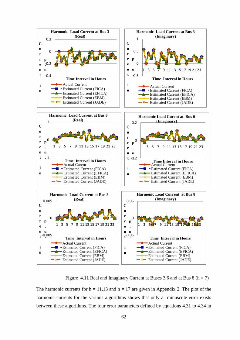
Figure 4.11 Real and Imaginary Current at Buses 3,6 and at Bus 8 (h = 7)

The harmonic currents for h = 11,13 and h = 17 are given in Appendix 2. The plot of the

harmonic currents for the various algorithms shows that only a minuscule error exists

between these algorithms. The four error parameters defined by equations 4.31 to 4.34 in

-0.4

-0.2

0

0.2

1 3 5 7 9 11 13 15 17 19 21 23

C

u

r

r

e

n

t

i

n

p

.

u



(Real)


-0.5

0

0.5

1

1 3 5 7 9 11 13 15 17 19 21 23

C

u

r

r

e

n

t

i

n

p

.

u



(Imaginary)


-1

0

1

1 3 5 7 9 11 13 15 17 19 21 23

C

u

r

r

e

n

t

i

n

p

.

u



(Real)

Actual CurentEstimated Current (FICA)Estimated Current (EFICA)Estimated Current (EBM)Estimated Current (JADE)

-0.2

0

0.2

1 3 5 7 9 11 13 15 17 19 21 23

C

u

r

r

e

n

t

i

n

p

.

u


Harmonic Load Curent at Bus 6

(Imaginary)


-0.005

0

0.005

1 3 5 7 9 11 13 15 17 19 21 23

C

u

r

r

e

n

t

i

n

p

.

u



(Real)


-0.05

0

0.05

1 3 5 7 9 11 13 15 17 19 21 23

C

u

r

r

e

n

t

i

n

p

.

u



(Imaginary)


66

Section 4.5.1.3 is evaluated for the IEEE 14 Bus System and is shown in Tables 4.6 -

4.11. From the tables it is observed that at Buses 3, 6 and 8 for harmonic frequencies h =

5, 7, 11 and 17 EBM has the lowest AAPE error. At Buses 3 and 6 for h = 13 JADE has

the lowest AAPE error and at Bus 8 EFICA has the lowest AAPE error for h = 13.

Hence, at varying harmonic frequencies the least AAPE error is not consistent for the four

bus system as well as the IEEE 14 bus system. This shows that an estimator may be

required to select the best ICA algorithm for both the interconnected systems.

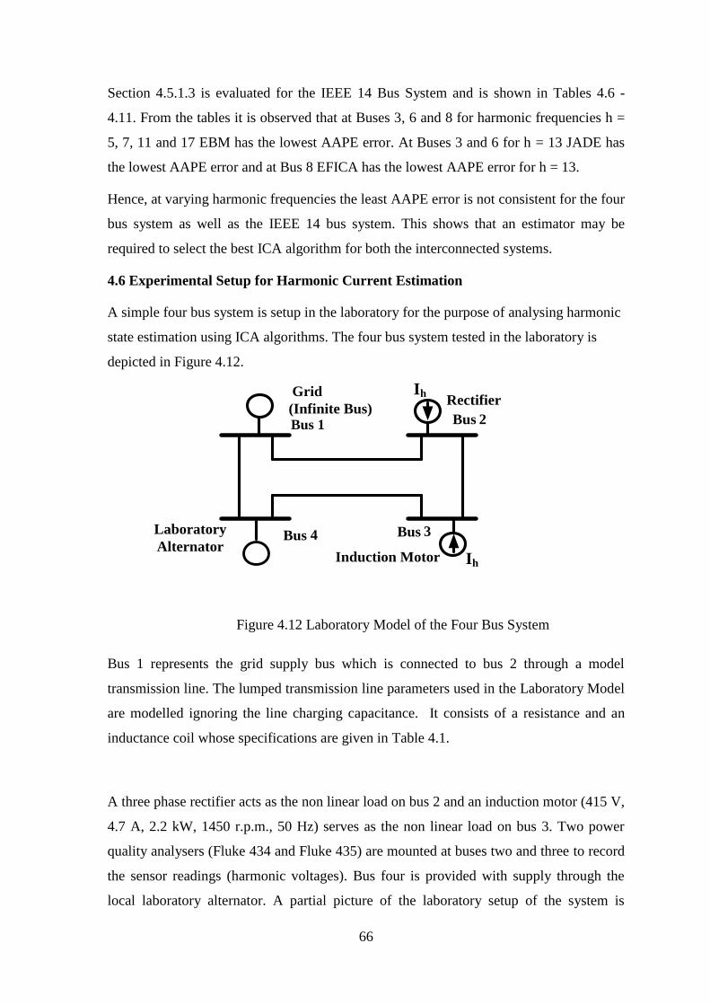
4.6 Experimental Setup for Harmonic Current Estimation

A simple four bus system is setup in the laboratory for the purpose of analysing harmonic

state estimation using ICA algorithms. The four bus system tested in the laboratory is

depicted in Figure 4.12.

Figure 4.12 Laboratory Model of the Four Bus System

Bus 1 represents the grid supply bus which is connected to bus 2 through a model

transmission line. The lumped transmission line parameters used in the Laboratory Model

are modelled ignoring the line charging capacitance. It consists of a resistance and an

inductance coil whose specifications are given in Table 4.1.

A three phase rectifier acts as the non linear load on bus 2 and an induction motor (415 V,

4.7 A, 2.2 kW, 1450 r.p.m., 50 Hz) serves as the non linear load on bus 3. Two power

quality analysers (Fluke 434 and Fluke 435) are mounted at buses two and three to record

the sensor readings (harmonic voltages). Bus four is provided with supply through the

local laboratory alternator. A partial picture of the laboratory setup of the system is

Laboratory

Alternator

Bus

2

Bus 3

Ih

Grid

(Infinite Bus)

Rectifier

Induction Motor

Bus 4

Ih

Bus 1

67

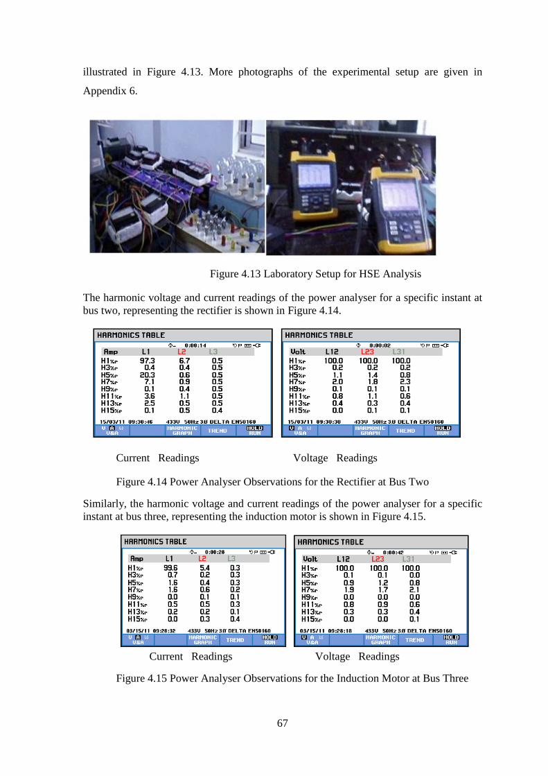
illustrated in Figure 4.13. More photographs of the experimental setup are given in

Appendix 6.

Figure 4.13 Laboratory Setup for HSE Analysis

The harmonic voltage and current readings of the power analyser for a specific instant at

bus two, representing the rectifier is shown in Figure 4.14.

Current Readings Voltage Readings

Figure 4.14 Power Analyser Observations for the Rectifier at Bus Two

Similarly, the harmonic voltage and current readings of the power analyser for a specific

instant at bus three, representing the induction motor is shown in Figure 4.15.

Current Readings Voltage Readings

Figure 4.15 Power Analyser Observations for the Induction Motor at Bus Three

68

The power analysers record only the magnitudes of the electrical quantities. The two

non-linear loads represent customer loads which undergo random fluctuations. These

random variations are recorded as sensor readings every two minutes at buses two and

three. The current magnitude evaluation is done by loading these 720 readings, taken at

every two minutes into Microsoft Excel and importing them to MATLAB where the ICA

algorithms are applied to the laboratory four bus model. The unknown currents at buses

two and three are thus determined and portrayed in Figures 4.16 and 4.17 for harmonic

frequencies 5 and 7 respectively. The estimated currents for this system for h = 11 and h

= 13 are shown in Appendix 3. The harmonic content at buses one and four is negligibly

small.

Figure 4.16 Current Magnitude at Bus 2 and Bus 3 at h = 5

Figure 4.17 Current Magnitude at Bus 2 and Bus 3 at h = 7

-1

0

1

1 3 5 7 9 11 13 15 17 19 21 23

C

u

r

r

e

n

t

i

n

A


Harmonic Load Current at Bus

2(Rectifier)


0

0.2

1 3 5 7 9 11 13 15 17 19 21 23

C

u

r

r

e

n

t

i

n

A



(Induction Motor)


0

0.5

1 3 5 7 9 11 13 15 17 19 21 23

C

u

r

r

e

n

t

i

n

A Time Interval in Hours


Bus 2(Rectifier)


0

0.1

1 3 5 7 9 11 13 15 17 19 21 23

C

u

r

r

e

n

t

i

n

A Time Interval in Hours


(Induction Motor)


70

The current magnitudes with h = 5 for both the loads agree well with the actual values.

The error is computed in terms of maximum absolute error (MAE), mean absolute error

(AME) and mean square error (MSE) for the laboratory model as defined in Section

4.5.1.3.

The effect of the errors defined in Section 4.5.1.3 for the various algorithms at both the

buses are given in Table 4.12 and in Table 4.13.

A comprehensive study of these tables illustrates the performance edge of EBM algorithm

over the other three ICA algorithms for h = 7 and h=11 at Bus 2 and for h=5 at both the

buses. However, for the harmonic frequency h=13, EFICA has better performance at Bus

2 and at h=7 its values are lower at Bus 3. The FICA has lower error values for h=11 and

h=13 at Bus 3. This proves the inconsistent nature of the ICA algorithms at various

harmonic frequencies and thereby establishes the need of an optimal estimator for

choosing the best ICA algorithm for the laboratory model also.

4.7 Integrated Kalman-ICA for Harmonic Current Estimation

An analysis of the simulation results of the four ICA algorithms in Section 4.5.1.3 and

section 4.5.2 indicates that the performance of the four ICA algorithms is not consistent at

the various harmonic frequencies considered. A similar observation is also made from the

error parameter calculation of the laboratory model in section 4.6.

The best ICA algorithm is chosen based on the lowest AAPE error as defined by equation

4.34 and the corresponding mixing matrix is referred to as the best mixing matrix (BMM)

and is denoted as Wbb. Next, the author proposes to process Wbb by a Kalman Filter to

obtain the final estimated harmonic current. The advantage of the Kalman Filter is that it

is an optimal estimator which attempts at reducing all forms of error.

The Kalman estimator [15] addresses the problem of estimating the state of any discrete

process that is governed by the linear stochastic difference equation.

(4.35)

(4.36)

1 k k k k k kx A x B u w

k k ky Hx

71

The random variables and represent the process and measurement noise. The

random variables and are denoted by process noise covariance Qk and

measurement noise covariance Rk respectively. Though the matrices Qk and Rk change

with each time step or measurement, in this work they are assumed to be constant.

The n×n matrix A in the difference equation (4.35) relates the state at the time step k-1

to the state at the current step k, in the absence of either a driving function or process

noise. The m×n matrix H in the measurement equation (4.36) relates the state to the

measurement yk. In practice H might change with each time step or measurement, but

here it is assumed to be a constant.

The equations (4.35) and (4.36) are employed to formulate the predict and update

equations.

The predicted state is given by:

(4.37)

The predicted variance matrix is as follows:

(4.38)

Equations (4.37) and (4.38) represent the predict equations for the Kalman Filter.

The optimal gain Kk is defined to minimise the error covariance and is given as:

(4.39)

Using the observation vector yk, the updated state estimate is:

(4.40)

The updated estimate variance matrix is:

(4.41)

kw k

kw k

x xk|k 1 k 1|k 1

TP A P A Qk|k 1 k k 1|k 1 k k

Pk|k

TT 1K P H (HP H R)k k|k 1 k|k 1

x x K (y Hx )k|k k|k 1 k k k|k 1

Pk|k

P (I K H)Pk|k k k|k 1

72

Equations (4.39) – (4.41) represent the update equations of the Kalman Filter. The

subscripts k|k denotes the current state, k|k-1 implies the intermediate state and k-1|k-1

represents the previous state. With proper model of the state process and the

measurement process and using equations (4.37) – (4.41) the Kalman filter can be used in

any application for tracking. The observation vector is the sensor readings at a

specific frequency , the measurement matrix H is represented by BMM and the updated

state estimate is the harmonic current at a specific harmonic frequency ‗h‘.The

harmonic current at the HIBs are finally got as the state estimates of the Kalman Filter.

The harmonic current estimation sequence using the integrated Kalman-ICA (IKICA)

method is represented in Figure 4.18.

Figure 4.18 Harmonic State Estimation Sequence using IKICA algorithm

yk

xk|k

73

The harmonic current estimation algorithm is implemented for the four bus system

described in Section 4.5.1 and the BMM is processed with a Kalman Filter and the

AAPE error with BMM and the Kalman Filter is indicated for various harmonic

frequencies in Table 4.14.

Table 4.14 AAPE Error for IKICA Method at Various ‗h‘ for Four Bus Model

The values of the AAPE error in Table 4.14 correspond to the lowest values of the ICA

algorithms which is also the output of the Kalman Filter at the respective harmonic

frequencies ‘h‘. It is found that at Bus 2, the EBM algorithm has the lowest AAPE error

at h= 5, 7 and 13 and at Bus 3 it has lowest error for harmonic frequencies of the order 5,

7, 13 and 17. FICA has the lowest AAPE error at h = 11 for both the buses. The lowest

AAPE error at Bus 2 for h = 17 is exhibited by EFICA algorithm. The inconsistent

behaviour of the ICA algorithms is due to the variations in the probability distribution of

the current sources. The discrepancy is cleared by using a Kalman Filter as the optimal

estimator which results in the lowest error at all harmonic frequencies for the simulated

four bus model.

Similarly, the IKICA algorithm could be employed for the system explained in Section

4.5.2 and section 4.6.

4.8 Harmonic Voltage Estimation

Some loads like electric arc furnace and PWM inverters generate voltage harmonics on a

large scale. Arc Furnaces generate even order harmonics and certain odd order harmonics

not commonly present in other loads. When harmonics exist at only one bus and the

remaining buses do not contribute to the harmonics, even though the harmonics spreads in

the network it is observed that most of the ICA algorithms fail as they are originally

crafted for separation of two or more signals. The non Gaussianity based Efficient

h' Bus 2 Bus 3

5 2.234 0.878

7 0.186 0.484

11 0.012 0.242

13 0.3659 0.2482

17 2.00E-04 0.0004

74

Variant Fast ICA(EFICA) and its related higher versions like COMBI and Multi COMBI

break down under this condition[72].

It is necessary to develop a new algorithm or a modification of existing algorithm for

precise estimation of single source harmonics generation bus. For this purpose, three

types of time structured ICA algorithms are investigated. One of these is JADE which is

found to be precise for such a case. One of the most accurate ICA algorithms called as

EBM is also analysed in the work for single source estimation. But a deeper analysis

indicates that this algorithm is not appropriate for voltage harmonic estimation of non

linear loads like arc furnaces which have considerable harmonic content at certain non –

existent frequencies like h=2, 3 ,4, etc. Hence, for the estimation of voltage harmonics a

combination of FICA and WASOBI called as FIWAS is attempted for voltage estimation.

4.8.1 Four Bus Model

The four bus test system comprises of two generators, two linear loads, two non linear

loads and four transmission lines linking the four buses. The four bus model is a modified

model given in [73] and is shown in Figure 4.19.

Figure 4.19 Four Bus Test System with Harmonic Voltage Sources

The transmission line parameters used for simulation are as specified in Table 4.1. The

harmonic voltage injected into the system is represented by harmonic voltage source, one

each at buses two and three, whose modelling is given for Pulse Width Modulation

(PWM) Inverter [63] and arc furnace [64].

G

G

Bus 1Bus 2

Bus 3

Bus 4

L3

L2

Vh

Vh

Arc

Furnace

PWM

Inverter

75

4.8.2 Generation of Data

The methodology employed for the generation of observation data (harmonic current) is

as follows:

1. The linear loads and the other power system components of the four bus

system are modelled as constant impedance loads as in [73]. The

harmonic sources are modelled as harmonic sources in [63, 64]. Thus the

admittance of the test system is formulated for a specific harmonic

frequency say (h=5).

2. The harmonic voltage of PWM and the arc furnace at buses 2 and 3 are

computed at h=5 frequency while the harmonic voltage values at the

remaining buses are taken as zero and a single harmonic current data is

generated for the system at h=5.

3. A random profile for the various buses is modelled using the Markov

model based on Poisson distribution concept for the four bus system.

Using this profile, the harmonic voltage data is generated at buses two and

three for 1440 readings. Substituting these readings for Vbh and Yh in the

equation (3.35) defined as: Ibh=Yh Vbh, 1440 values for Ibh are obtained at

h=5.

4. Steps (1), (2) and (3) are repeated for h=7. The corresponding Ibh data

generated are defined as the harmonic current sensor readings. The arc

furnace generates appreciable harmonics at h=2, 3 and h=4, whereas at

these harmonic frequencies the PWM inverter generates negligible

harmonic voltage. With the harmonic voltage value only at Bus 3 and the

remaining harmonic voltages as zero, the harmonic current data is

generated at h=2 for the four bus system. Using step (3) 1440 values of

harmonic current data for the arc furnace is generated. Similarly harmonic

current data is generated for h=3 and h=4 respectively.

76

4.8.3 Methodology of Implementation

Once the voltage sensor readings for the four bus test system is generated the various

ICA algorithms are applied in the following manner:

Step 1: Determine the Harmonic Injection Buses (HIB) using total voltage harmonic

distortion.

Step 2: Obtain the sensor readings at the bus three and substitute the sensor reading at

bus 2 as 0.00002, instead of zero.

Step 3: Apply FICA algorithm for the harmonic voltage sensor readings (h = 5).

Step 4: Compute the error coefficients MAE, AME, MSE and AAPE as defined in section

4.5.4 for FIWAS algorithm.

Step 5: Repeat step (2) and step (3) for JADE and EBM algorithms.

Step 6: Repeat for all harmonics (h = 2, 3, 4, 5 and 7).

4.8.4 Simulation Results

The sensor readings are recorded and analysed on a specific day. The estimated voltages

Veh for that particular day are portrayed in Figures 4.20 and 4.21 for buses two and three

which have the non linear loads. The real and imaginary components of harmonic

voltages for the three algorithms - FIWAS, EBM and JADE are thus plotted.

0

0.05

1 3 5 7 9 11131517192123

V

o

l

t

a

g

e

i

n

p

.

u


Harmonic Load Voltage at

Bus 3(Real)

Actual VoltageEstimated Voltage (FIWAS)Estimated Voltage (EBM)Estimated Voltage (JADE)

0

0.01

1 3 5 7 9 11 13 15 17 19 21 23

V

o

l

t

a

g

e

i

n

p

.

u


Harmonic Load Voltage at Bus 3

(Imaginary)


77

Figure 4.20 Harmonic Voltages at Bus 3 for h = 2 and h = 3

Figure 4.21 Harmonic Voltages at Bus 2 and Bus 3 for h = 5

The harmonic voltages at Bus 2 and Bus 3 for h = 4 and h = 7 are shown in Appendix 4.

0

0.5

1 3 5 7 9 11 13 15 17 19 21 23

V

o

l

t

a

g

e

i

n

p

.

u

.



Bus 3(Real)


0

0.05

1 3 5 7 9 11 13 15 17 19 21 23

V

o

l

t

a

g

e

i

n

p

.

u



Bus 3(Imaginary)

Actual VoltageEstimated Voltage(FIWAS)Estimated Voltage(EBM)Estimated Voltage(JADE)

-0.5

0

0.5

1 3 5 7 9 11 13 15 17 19 21 23

V

o

l

t

a

g

e

i

n

p

.

u

.


Harmonic Load Voltage at Bus 2

(Real)

Actual Voltage

Estimated Voltage (FIWAS)

Estimated Voltage (EBM)

Estimated Voltage (JADE)

-0.1

0

0.1

1 3 5 7 9 11 13 15 17 19 21 23

V

o

l

t

a

g

e

i

n

p

.

u



Bus 2(Imaginary)

Actual Voltage




-0.5

0

0.5

1 3 5 7 9 11 13 15 17 19 21 23

V

o

l

t

a

g

e

i

n

p

.

u

.



Bus 3(Real)


-0.1

0

0.1

0.2

1 3 5 7 9 11 13 15 17 19 21 23

V

o

l

t

a

g

e

i

n

p

.

u

.



Bus 3(Imaginary)

Actual Voltage




80

From the graphs, the results of both the algorithms appear to be identical. Hence the

performance is gauged in terms of the four error quantities defined by equations 4.31 to

4.34.

The effect of the errors defined in these equations for the FIWAS, EBM and JADE

algorithms at buses 2 and 3 are given in Tables 4.15 - 4.18.

A complete examination of these tables illustrates the performance edge of FIWAS

algorithm for h = 2, 3 and h = 5 at Bus 3 and for h = 7 at Bus 3. JADE which is known for

its accurate performance has the lowest error at h = 5 for Bus 2 and for h = 7 for Bus 3.

The use of the IKICA algorithm for the four bus system with the harmonic voltage

sources is thus justified as the two ICA algorithms show incoherent behaviour at the

harmonic frequencies considered.

4.9 Harmonic Voltage and Current Estimation: Harmonic voltage and harmonic

current producing loads may coexist in many interconnected systems. Hence a combined

effect of harmonic current producing loads like SVC and HVDC and harmonic voltage

producing loads like arc furnace and PWM Inverters is investigated on an IEEE 14 Bus

System. The combined effect of harmonic voltage and current sources is analysed in this

section using three ICA algorithms- FIWAS, EBM and JADE. Also, the principle of

superposition is applied to the IEEE 14 Bus System to estimate the harmonic voltage and

current at the suspicious buses.

4.9.1 IEEE 14 Bus model The IEEE-14 bus system used as the test sample for the

Figure 4.22 IEEE 14 Bus Test Systems with Harmonic Voltage and Current Sources

2

1

12

13

14

1110

3

5

6

4

9

8

G

G

CHVDC

SVC

7

PWM

INVERTER

ARC

FURNACE

81

work is shown in Figure 4.22. The IEEE 14 bus test system [75] comprises of four non

linear loads at buses 3, 6, 8 and 10. These non linear loads are represented by SVC,

HVDC, PWM Inverter and the arc furnace. The SVC at bus 3 and HVDC at bus 8

represent the harmonic current sources. The PWM inverter at bus 6 and the arc furnace at

bus 10 represent the harmonic voltage sources respectively. The IEEE-14 bus system is to

be modelled with the power system components like transmission lines, linear loads and

the current and voltage sources for the generation of observation data in order to apply the

ICA analysis.

4.9.2 Generation of Data

The methodology employed for the generation of observation data (harmonic

voltage/harmonic current) is as follows:

1. The linear loads and the other power system components of the IEEE 14

bus system are modelled as constant impedance loads as in [73]. The

harmonic sources are modelled as harmonic sources in [60, 61, 62 and

63]. Thus the admittance of the test system is formulated for a specific

harmonic frequency say (h = 5).

2. The harmonic current of SVC and HVDC at buses 3 and 8 are

computed at harmonic frequency (h = 5) while the harmonic current

values at the remaining buses are taken as zero and a single harmonic

voltage data is generated for the system at h = 5.


model based on Poisson distribution concept for the IEEE 14 bus system.

Taking into account, one reading in one minute for a specific day the

values of 1440 readings are to be extrapolated for all buses.

4. Using this profile, the harmonic current data at all buses in all lines and

loads is generated for 1440 readings. Substituting these readings for Ibh

and Zh (inverse of admittance of the test system) in the equation (2)

defined as: Vbh=ZhIbh, 1440 values for Vbh are obtained at h = 5, for b = 1

to 14.

82

5. Steps (1) to (4) are repeated for h = 7, 11, 13 and 17 .The corresponding

Vbh data generated are defined as the harmonic voltage sensor readings.

6. The harmonic voltage of PWM and the arc furnace at buses 6 and

10[63,64] are computed at h = 5 frequency while the harmonic voltage

values at the remaining buses are taken as zero and a single harmonic

current data is generated for the system at h = 5.


model concept for the IEEE 14 bus system. Using this profile, the

harmonic voltage data is generated for 1440 readings. Substituting these

readings for Vbh and Yh in the equation (3) defined as: Ibh=Yh Vbh, 1440

values for Ibh are obtained at h = 5.

8. Steps (1), (6) and (7) are repeated for h = 7, 11, 13 and 17. The

corresponding Ibh data generated are defined as the harmonic current

sensor readings.

4.9.3 Methodology of Implementation:

Once the voltage and current sensor readings for the IEEE 14 bus system is generated the

various ICA algorithms are applied in the following manner:

Step 1: Determine the Harmonic Injection Bus (HIB) using total voltage

harmonic distortion and total current harmonic distortion

Step 2: Obtain the voltage sensor readings at buses three and eight and the

current sensor readings at buses six and ten.

Step 3: Apply FIWAS algorithm for the harmonic voltage sensor readings

(h = 5).

Step 4: Compute correlation coefficient for this algorithm.

Step 5: Repeat step (2) and step (3) for JADE and EBM algorithms.

Step 6: Repeat for all harmonics.

Step 7: Repeat from step 3 to step six for current sensor readings.

It is evident from step 3 and step 7 that each ICA algorithm need to be

applied twice which calls for applying the superposition principle to

83

equation (2) and (3) and thereby analysing the effect of current/voltage

harmonics based on IEEE 512-1992 [1].

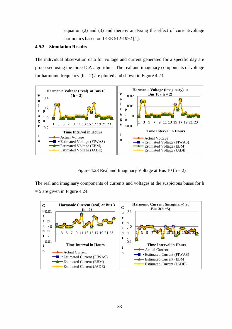
4.9.3 Simulation Results

The individual observation data for voltage and current generated for a specific day are

processed using the three ICA algorithms. The real and imaginary components of voltage

for harmonic frequency (h = 2) are plotted and shown in Figure 4.23.

Figure 4.23 Real and Imaginary Voltage at Bus 10 (h = 2)

The real and imaginary components of currents and voltages at the suspicious buses for h

= 5 are given in Figure 4.24.

-0.2

0

0.2

0.4

1 3 5 7 9 11 13 15 17 19 21 23

V

o

l

t

a

g

e

i

n

p

.

u

.


Harmonic Voltage ( real) at Bus 10

( h = 2)


-0.01

0

0.01

0.02

1 3 5 7 9 11 13 15 17 19 21 23

V

o

l

t

a

g

e

i

n

p

.

u

.


Harmonic Voltage (imaginary) at

Bus 10 ( h = 2)


-0.01

0

0.01

1 3 5 7 9 11 13 15 17 19 21 23

C

u

r

r

e

n

t

i

n

p

.

u

.


Harmonic Current (real) at Bus 3

(h =5)

Actual Current

Estimated Current (FIWAS)

Estimated Current (EBM)

Estimated Current (JADE)

-0.1

0

0.1

1 3 5 7 9 11 13 15 17 19 21 23

C

u

r

r

e

n

t

i

n

p

.

u

.


Harmonic Current (imaginary) at

Bus 3(h =5)

Actual Current

Estimated Current (FIWAS)

Estimated Current (EBM)

Estimated Current (JADE)

84

Figure 4.24 Real and Imaginary Current at Bus 3 and Bus 8 (h = 5)

Figure 4.25 Real and Imaginary Voltage at Buses 6 and 10 (h = 5)

From the graphs in Figure 4.23 it is observed that for h = 2, FIWAS and JADE have

similar performance and separate the estimated voltage accurately. However, EBM does

not provide reliable results for h = 2. But for h = 5, shown in Figure 4.24 and 4.25 it is

found that FIWAS and EBM have a similar level of performance and JADE has a lower

degree of performance. In order to analyse the separation quality of the algorithms better,

various correlation coefficients are formulated [76].Though several methods of estimating

the correlation exist, the Spearman‘s coefficient and the concurrent deviation method are

-0.5

0

0.5

1 3 5 7 9 11 13 15 17 19 21 23

C

u

r

r

e

n

t

i

n

p

.

u


Harmonic Current (real) at Bus 8

(h =5)

Actual CurrentEstimated Current (FIWAS)Estimated Current (EBM)Estimated Current (JADE)

-1

0

1

1 3 5 7 9 11 13 15 17 19 21 23

C

u

r

r

e

n

t

i

n

p

.

u

.


Harmonic Current (imaginary) at

Bus 8(h =5)

Actual CurrentEstimated Current (FIWAS)Estimated Current (EBM)Estimated Current (JADE)

-0.5

0

0.5

1 3 5 7 9 11 13 15 17 19 21 23

V

o

l

t

a

g

e

i

n

p

.

u


Harmonic Voltage (real ) at Bus 6

( h= 5 )


-2

0

2

1 3 5 7 9 11 13 15 17 19 21 23

V

o

l

t

a

g

e

i

n

p

.

u

.



Bus 6 ( h = 5)


0

1

1 3 5 7 9 11 13 15 17 19 21 23

V

o

l

t

a

g

e

i

n

p

.

u

.


Harmonic Voltage (real) at Bus 10

(h = 5)

Actual Voltage



-2

0

1 3 5 7 9 11 13 15 17 19 21 23V

o

l

t

a

g

e

i

n

p

.

u



Bus 10 (h = 5)


85

used for comparison of the separation quality of the three algorithms. Spearman‘s

coefficient of correlation is a non –parametric distribution based coefficient of

correlation. It is based on the difference of ranks between two variables and is defined as:

2

2

1 1

1 61

R R

DR

N N

(4.42)

where D is the difference between the ranks of two consecutive samples of the

random variable and NR1 is a value equal to the number of differences in the entire data

set. The spearman‘s coefficient is applicable only to limited number of samples as the

calculation tends to become tedious. So the above values may not convey much

information as the sample size in the work is 1440. Hence a modified form of correlation

estimation termed as Concurrent Deviation method is used for defining the separation

quality of the three algorithms. This method is based on finding the direction of change

of either of the two random variables and is given by:

2

2 c r

r

C nR

n

(4.43)

In the equation (4.43) R2 represents the coefficient of correlation. Cc denotes the number

of concurrent deviations or the number of positive signs obtained after multiplying the

direction change of the actual and estimated voltage variables and nr denotes the number

of pairs of observation compared.

The coefficient (R) for h = 5, 7 and 11 at buses 3, 6, 8 and 10 are tabulated in Tables 4.19

– 4.21 using the Spearman‘s coefficient and the concurrent deviation method for the

algorithms FIWAS, JADE and EBM.

Table 4.19 Correlation Coefficients at h=5 for IEEE -14 Bus System

Buses Correlation

Coefficients

Real Imaginary

FIWAS EBM JADE FIWAS EBM JADE

Bus 3 R1 0.987 0.981 0.979 0.989 0.985 0.977

R2 0.985 0.983 0.978 0.984 0.982 0.971

Bus 6 R1 0.984 0.982 0.976 0.985 0.981 0.973

R2 0.986 0.984 0.979 0.987 0.984 0.978

Bus 8 R1 0.985 0.983 0.973 0.986 0.979 0.981

R2 0.983 0.981 0.972 0.983 0.981 0.981

Bus 10 R1 0.982 0.98 0.974 0.982 0.981 0.976

R2 0.988 0.979 0.981 0.985 0.982 0.977

86


Buses Correlation

Coefficients

Real Imaginary


Bus 3 R1 0.984 0.986 0.975 0.988 0.984 0.978

R2 0.987 0.982 0.973 0.985 0.981 0.976

Bus 6 R1 0.986 0.981 0.975 0.986 0.983 0.975

R2 0.982 0.983 0.971 0.984 0.982 0.974

Bus 8 R1 0.988 0.984 0.972 0.981 0.976 0.981

R2 0.982 0.981 0.974 0.982 0.98 0.975

Bus 10 R1 0.986 0.98 0.977 0.984 0.983 0.974

R2 0.983 0.979 0.98 0.98 0.978 0.972


Buses Correlation

Coefficients

Real Imaginary


Bus 3 R1 0.986 0.985 0.975 0.985 0.982 0.973

R2 0.985 0.983 0.971 0.982 0.976 0.971

Bus 6 R1 0.984 0.982 0.974 0.986 0.982 0.972

R2 0.983 0.981 0.97 0.984 0.98 0.974

Bus 8 R1 0.985 0.984 0.976 0.981 0.972 0.97

R2 0.987 0.985 0.975 0.982 0.978 0.974

Bus 10 R1 0.986 0.98 0.971 0.984 0.981 0.975

R2 0.98 0.977 0.973 0.98 0.974 0.976

The closer the correlation coefficient is to 1 better is the separation index of the ICA

algorithm [77], as a value of one is the best separation. Thus, on comparing the

correlation coefficient at various harmonic frequencies, the performance edge of

FIWAS is observed for h = 5, 7 and 11.

4.10 Discussions

A comparative study of the four ICA algorithms indicates some significant findings on

each of the algorithms. The nature of the probability distribution of the harmonic source

plays a vital role in minimizing the error for the various ICA algorithms. The FICA

algorithm directly finds independent components of any non-Gaussian distribution using

any nonlinearity. This is in contrast to many algorithms, where some estimate of the

probability distribution function has to be first available, and the nonlinearity must be

chosen accordingly. Despite this, FICA is not suitable for finite samples of data.

87

EFICA has an advantage of adaptive choice of non linearity and it is applicable for finite

samples also. Further, EFICA exhibits lowest error for the generalized Gaussian

distribution. This has been forcefully brought out in this chapter through simulation of

the four bus model.

The advantage of JADE is that it works on cross-cumulants and hence one need not resort

to gradient descent algorithm with its attendant convergence problems. Further, the

algorithm does not require any parameter for tuning. A disadvantage of this approach is

that estimating a complete set of fourth order cross-cumulants requires storage of

cumulant matrices.

Being based on entropy bound minimization; the EBM algorithm has the clear advantage

of being applicable to a wide range of probability distributions. In addition, the algorithm

when applied leads to minimum deviation from the actual value.

The detailed simulation and experimental studies have been conducted to identify the best

ICA algorithm for harmonic source estimation. The same has been done for all the three

possible cases of harmonic current source, harmonic voltage source or both. Simulation

is conducted on 4 bus model and 14 bus model with non linear loads and experiment is

conducted on 4 bus laboratory model . In all the systems, four time structured ICA

algorithms are attempted to find the best ICA algorithm. This chapter reports the results

of the investigation and a critical comparative study of the ICA algorithms.

The analysis is made for different buses and different harmonic frequencies at each bus to

pick out the best ICA algorithm. AAPE values have been used as the figure of merit for

comparison.

Considering the four bus system, specifically the bus 2 with nonlinear loads connected to

it, all algorithms gave inconsistent performance for all the non triplen harmonics. (Vide

Table 4.2 for the AAPE error). FICA and EFICA algorithm gave the lowest error for

harmonic frequencies 11 and 13 respectively. In contrast, EBM algorithm gave the lowest

error for the more crucial frequencies 5, 7 and 13.

With non linear load at bus 3 of the four bus system, EBM algorithm once again gave the

lowest error in all frequencies other than 11th

order harmonic frequency. This again

clearly confirms the superior performance of EBM algorithm. Similarly, for the 11th

order

frequency, FICA gave the lowest error.

Considering the 14 bus system none of the algorithms show superior performance at all

harmonic frequencies at buses 3,6 and 8 as shown in Tables 4.6, 4.8 and 4.10.Here also

88

EBM algorithm is the best bet as it has given the lowest error at buses 3,6 and 8 for all

harmonic frequencies 5, 7,11 and 17 except 13.

For 13th

order harmonic frequency, JADE has the lowest error at buses 3 and 8 and for

the same harmonic frequency EFICA has the lowest error at bus 8.

These results points to the necessity of further processing to select the most accurate

algorithm. A Kalman Filter is used as an optimal estimator to process the best mixing

matrix for harmonic current estimation. By processing using Kalman Filter as given in

table 4.14, the optimal ICA algorithm for the four bus model turns out to be the EBM

algorithm for most of the cases. However, for few harmonic frequencies FICA and

EFICA are the optimal choice for harmonic current estimation.

The harmonic voltage estimation on a 4 bus system is carried out which indicates the

advantage of the FIWAS algorithm for such an estimation. It also shows that the EBM

algorithm is not suited for solitary harmonic voltage source estimation. Though the JADE

algorithm is one of the most accurate ICA algorithms, it has a lower performance than

FIWAS for harmonic voltage estimation as observed from Table 4.17. Also for the

harmonic frequencies considered – 2, 3 and 4 which are the non conventional harmonic

frequencies, at bus 3 FIWAS has least error for harmonic frequency 2 and 3, whereas

JADE has the lowest error for 4th

order harmonic frequency.

The parameters like MAE, AME, MSE and AAPE suggest further probing of a better

figure of merit to select the foremost ICA algorithm. Correlation Coefficient is another

figure of merit for selecting the most apt ICA algorithm with the least error. In order to

consider the most advantageous ICA algorithm, the highest value of the correlation

coefficient is examined for the combined harmonic voltage and harmonic current

estimation on an IEEE 14 bus. The correlation coefficients tabulated in Tables 4.19 - 4.21

point to the unsurpassed accomplishment of the FIWAS algorithm over the EBM

algorithm for majority of the harmonic frequencies.

The investigations establish EBM algorithm as having superior performance for harmonic

current estimation. However, for solitary harmonic voltage and the combined harmonic

voltage and current estimation FIWAS algorithm has the superior edge.

4.11 Conclusions

The results of the Harmonic State Estimation for current and voltage with the help of four

time structured algorithm is compared in this chapter in order to select the best ICA

89

algorithm. Since no algorithm is found to be universally the best algorithm, further

processing is carried out by an optimal estimator like Kalman Filter. Also, correlation

coefficients are formulated to evaluate the best ICA algorithm. By and large it is found

that EBM is the best ICA algorithm for harmonic current and voltage estimation. The

existence of sufficient measurements to carry out the state estimation is examined in the

next chapter.

Date post:	05-Apr-2018
Category:	Documents
Upload:	truongkhanh
View:	223 times
Download:	0 times

HARMONIC STATE ESTIMATION - Shodhgangashodhganga.inflibnet.ac.in/bitstream/10603/8430/16/16_chapter...

Documents