Introduction Over the past 30 years, economic activity has become less volatile in most G-7 countries. In the United States, for example, the stan- dard deviation of the growth rate of GDP averaged over four quarters was one-third less during 1984 to 2002 than it was during 1960 to 1983. This decline in volatility is widespread across sectors within the United States and is also found in the other G-7 economies, although the timing and details differ from one country to the next. Interest- ingly, despite these changes and increasing international economic integration, output fluctuations have not become more correlated or synchronized across countries. Much has been written about the possible causes of this “great moder- ation.” In this paper, we review existing evidence and present some new evidence on these causes. Our main focus is on the hypothesis that the great moderation is a happy byproduct of improved monetary policy. For the United States (on which the most data are available and the most has been written), monetary policy is generally thought to have been too accommodative during the 1960s and 1970s (DeLong 1997, Romer and Romer 2002, Sargent 1999); this changed in 1979, and for the 1980s and 1990s the Fed showed a commitment to maintaining low inflation. James H. Stock Mark W. Watson Has the Business Cycle Changed? Evidence and Explanations 9
Transcript
Introduction
Over the past 30 years, economic activity has become less volatilein most G-7 countries. In the United States, for example, the stan-dard deviation of the growth rate of GDP averaged over four quarterswas one-third less during 1984 to 2002 than it was during 1960 to1983. This decline in volatility is widespread across sectors within theUnited States and is also found in the other G-7 economies, althoughthe timing and details differ from one country to the next. Interest-ingly, despite these changes and increasing international economicintegration, output fluctuations have not become more correlated orsynchronized across countries.
Much has been written about the possible causes of this “great moder-ation.” In this paper, we review existing evidence and present some newevidence on these causes. Our main focus is on the hypothesis that thegreat moderation is a happy byproduct of improved monetary policy. Forthe United States (on which the most data are available and the most hasbeen written), monetary policy is generally thought to have been tooaccommodative during the 1960s and 1970s (DeLong 1997, Romer andRomer 2002, Sargent 1999); this changed in 1979, and for the 1980sand 1990s the Fed showed a commitment to maintaining low inflation.
James H. StockMark W. Watson
Has the Business Cycle Changed?Evidence and Explanations
9
If improved monetary policy tamed inflation, does it not stand toreason that it also produced the great moderation? Not necessarily. Therole for monetary policy in the great moderation is summarized inFigure 1, which plots the standard deviation of a measure economicactivity against the standard deviation of the rate of inflation. The actualvalues of these standard deviations depend on the structure of theeconomy, the shocks experienced by the economy, and the monetarypolicy followed by the Fed. Different rules produce different values forthese standard deviations, and the best that the policymaker can do,given the structure of the economy, is to reach the “frontier” representedby the solid line in Figure 1. The points B, C, and D are achieved bythree different policies on the frontier; none dominates the others, in thesense that none has both lower inflation and output volatility than theothers. Point A is within the frontier. If A represents the policy of the1960s and 1970s, inflation volatility could be reduced by moving to any
10 James H. Stock and Mark W. Watson
Figure 1Monetary Policy and the Variability of Output and Inflation
Points B, C, D are on the feasible frontier (solid line) representing the tradeoffbetween the standard deviation of inflation (σπ) and the standard deviation ofoutput (σy); points B, C, and D all have less inflation volatility than point A, whichis within the frontier. Point E is on a frontier that has shifted toward the origin fromthe original frontier.
E
D
C
B
A
point to its left, for example, to B, C, or D. Whether this shift alsoreduces output volatility depends on the details of the policy and on theworkings of the economy. If the shift is to B, output volatility dropsconsiderably; if it is to C, output volatility falls slightly; but if it is to D,output becomes more volatile. At this level of abstraction, improvedmonetary policy that reduces inflation variability might also reduceoutput variability, then again it might not. This all assumes that thefrontier has stayed fixed, but if shocks to the economy are smaller, or ifthe private sector becomes better at smoothing shocks, then the frontiershifts toward the origin and the policy that led to C would now lead toE: It would appear that the improved policy led to lower output volatil-ity, but most of the volatility reduction is the result of smallermacroeconomic shocks or structural changes in the economy.1
The empirical results in this paper suggest that improved monetarypolicy accounted for only a small fraction of the reduction in the vari-ance of output growth from the pre-1984 period to the post-1984period in the United States, and that the bulk of the great moderationarose from shifts in the frontier; in terms of Figure 1, we think that thepath “A-C-E” provides the most plausible description of the improvedmacroeconomic performance of the past two decades. This argumentrequires estimating how the post-1984 economy would have evolvedhad the monetary policy of the 1970s been in place, and to answer thisquestion we use four different modern econometric models, rangingfrom a backward-looking vector autoregression to a forward-lookingnine-equation dynamic stochastic general equilibrium model. Remark-ably, these different models lead to the same conclusion: Althoughimproved monetary policy played a key role in getting inflation undercontrol, it played, at best, a modest role in the great moderation. Thisconclusion is reinforced by the international evidence.
This leaves an important question: Why did the frontier shift in, andis this shift likely to be permanent or temporary? We conclude that partof the inward shift could be permanent, but the empirical evidencesuggests that much—half or more—of the great moderation could betemporary, the result of smaller macroeconomic shocks, in particular
Has the Business Cycle Changed? Evidence and Explanations 11
smaller common international shocks. Were these common interna-tional shocks to become again as large as they were in the 1970s,volatility would increase throughout the G-7 and the G-7 businesscycles would become more synchronized.
Before turning to the evidence, we make a few general commentsabout the analysis. Although we discuss aspects of changes in the busi-ness cycle for all the G-7 economies, because of data limitations andspace constraints, our discussion focuses primarily on the United States.Our interest is on changes in the business cycle; changes in time seriesproperties at very high frequencies can be the consequence of changes insurvey methods or other features not directly germane to business cycleanalysis, and structural economic changes that affect long-term growthrates, while certainly important, bear only indirectly on short-termmacroeconomic management. We therefore take Hall’s (2002) adviceand use transformations of the data that focus on fluctuations at busi-ness cycle frequencies. For real series, we examine four-quarter growthrates; for GDP, this is 100ln(GDPt /GDPt-4). Longer growth rates, whilealso of interest, reduce the number of non-overlapping observations.The models and analysis specific to the United States uses real GDP, butfor cross-country comparisons we use real GDP per capita.
Changes in the business cycle in the G-7, 1960-2002
The business cycle has changed in important ways over the past fourdecades: Output fluctuations have moderated, GDP growth is easier toforecast, and shocks to GDP are more persistent. Curiously, one thingthat has not changed is the degree of synchronization of business cyclesamong the G-7.
Widespread but varied reductions in output volatility
Perhaps the most striking change in the business cycle over the pastthree decades has been the dramatic decline in the volatility of GDPgrowth in most G-7 economies. In the United States, this “greatmoderation,” first documented by Kim and Nelson 1999 and
12 James H. Stock and Mark W. Watson
Has the Business Cycle Changed? Evidence and Explanations 13
Chart 1Four-Quarter Growth Rates of GDP per Capita
1960-6
-4
-2
0
2
4
6
8
10
12
1965 1970 1975 1980 1985 1990 1995 2000 2005
A. Canada
1960-6
-4
-2
0
2
4
6
8
10
12
1965 1970 1975 1980 1985 1990 1995 2000 2005
B. France
1960-6
-4
-2
0
2
4
6
8
10
12
1965 1970 1975 1980 1985 1990 1995 2000 2005
C. Germany
1960-6
-4
-2
0
2
4
6
8
10
12
1965 1970 1975 1980 1985 1990 1995 2000 2005
D. Italy
1960-6
-4
-2
0
2
4
6
8
10
12
1965 1970 1975 1980 1985 1990 1995 2000 2005
E. Japan
1960-6
-4
-2
0
2
4
6
8
10
12
1965 1970 1975 1980 1985 1990 1995 2000 2005
F. United Kingdom
1960-6
-4
-2
0
2
4
6
8
10
12
1965 1970 1975 1980 1985 1990 1995 2000 2005
G. United States
McConnell and Perez-Quiros 2000, is well characterized as a sharpreduction in the variance of GDP growth in the mid-1980s; usingdifferent econometric techniques and working independently, bothKim and Nelson 1999 and McConnell and Perez-Quiros 2000 esti-mate a break date of 1984.
This decline in cyclical volatility has occurred not just in the UnitedStates but, to varying degrees, in the other G-7 economies as well.Chart 1 plots the four-quarter growth rate of GDP for the G-7economies over the past four decades. As is summarized in Table 1, thestandard deviation of four-quarter GDP for France, Germany, Italy,Japan, the UK, and the United States over the period 1984-2002 is lessthan three-fourths what it had been during the earlier period, 1960-1983. Indeed, the variance of four-quarter GDP growth in these sixcountries fell by 50 percent to 80 percent.2
The estimates in Table 1 use the 1984 date of the volatility shift inthe United States, but this date or the single-break model might not beappropriate for other countries. In addition, the standard deviations inTable 1 might confound changes in the trend growth rate of output inthese countries with changes in business cycle fluctuations. In fact,Germany, France, Italy, and Japan grew much more rapidly in the1960s, when postwar reconstruction was still under way, than in thepast two decades, and the standard deviations reported in Table 1 inprincipal contain the two effects of changing cyclical fluctuations anddecadal changes in the mean growth rate. It is therefore desirable toobtain alternative estimates of the time path of volatility, which do notrely on a single break date and are robust to movements in the long-term growth rate of output.
Accordingly, Chart 2 plots estimates of the instantaneous standarddeviation of four-quarter GDP growth in these economies. These esti-mates are based on an autoregressive model with time-varyingcoefficients that allow for a long-run GDP growth rate that varies overtime.3 These estimated volatility paths show a broadly similar pattern asTable 1, although some details differ. The estimates for Canada in
14 James H. Stock and Mark W. Watson
Chart 2 show a large decline in volatility, but this decline occurs in theearly 1990s, not the mid-1980s. The estimates for France suggest thatthere has been little change in volatility over most of the past 30 years.The volatility decline for Germany is very large and, according to theChart 2 estimates, is nearly a straight-line decrease. The volatilitydecline in Italy and the UK preceded that in the United States, whilein Japan volatility is estimated to have fallen in the 1970s but thenincreased again in the late 1990s. In short, while there is clear statisti-cal evidence of a reduction in volatility in (at least) Germany, Italy,Japan, the UK, and the United States, the particulars of magnitude andtiming differ substantially from one country to the next.
A related aspect of the great moderation is that, at least in theUnited States, expansions have grown longer and recessions shorter;the 120-month U.S. expansion of the 1990s is the longest in the 140years covered by the NBER chronology, the 92-monthly expansion ofthe 1980s is the third-longest, and the two post-1984 recessions wereboth short, only eight months. These changes have a straightforward
Has the Business Cycle Changed? Evidence and Explanations 15
Table 1Changes in Volatility of Four-Quarter Growth of Real GDP
Per Capita in the G-7, 1960-1983 and 1984-2002
Standard Standard std. dev. 84-02 variance 84-02deviation, deviation, std. dev. 60-83 variance 60-83
Notes: Entries in the first two columns are the standard deviations of the four-quarter growth in GDPover the indicated time periods. The third column contains the ratio of standard deviation in the secondcolumn to that in the first; the final column presents the square of this ratio, which is the ratio of thevariances of four-quarter GDP growth in the two periods. Data sources are given in the Data Appendix.
interpretation. If the long-term growth rate of output is constant andits variance decreases, then (all else equal) periods of negative growthbecome fewer and farther apart. Because recessions are periods ofnegative growth, a moderation in output volatility with no change inthe mean growth rate implies, in this mechanical sense, shorter reces-sions and longer expansions.4
GDP growth is more forecastable and persistent
The innovations in GDP growth in the G-7 have also become smallerin the post-1984 period, and in this sense GDP growth has becomeeasier to forecast using simple time series models. Table 2 summarizessome results for simulated forecasts of quarterly GDP growth usingunivariate time series models. The first pair of columns reports the stan-dard error of the regression for autoregressions with four lags; thisone-quarter-ahead standard error fell in all seven countries, in severalcases by more than one-third. These autoregressions could not have beenused for forecasting because they were estimated using data beyond theforecast period. A better way to simulate real-time forecasting is to esti-mate a different autoregression at each date, where the estimates arebased on a moving window of data that would have been available at thedate the forecast is made. The root mean squared error of the resultingpseudo out-of-sample forecasts produced this using an eight-yearwindow is summarized in the third and fourth column. The forecastroot mean squared errors are somewhat larger than the standard error ofthe regressions in the first two columns over the post-1984 sample inpart because the autoregressions in the third and fourth columns wereestimated using fewer observations. As in the first two columns,however, the root mean squared forecast errors are substantially less post-1984 than pre-1984.5
Table 2 also reports a measure of the change in the persistence of ashock to GDP growth, specifically the sum of the autoregressive coeffi-cients; the inverse of one minus this sum is the cumulative effect of aGDP forecast error on the long-term forecast of GDP, so an increase inthis sum implies an increase in the persistence of a univariate innovation
Has the Business Cycle Changed? Evidence and Explanations 17
in GDP. In Canada, France, the UK, and, to a lesser extent, Italy and theUnited States, the sum of the autoregressive coefficients increased fromthe first period to the second.
Sectoral volatility has decreased
Is the reduction in volatility evident in GDP growth widespreadthroughout the U.S. economy, or is it limited to certain sectors orseries? This question is addressed in Table 3 for 22 major U.S. seriesconsisting of the main NIPA aggregates and selected other macroeco-nomic time series. As can be seen in Table 3, the volatility of 21 ofthese 22 series fell in the post-1984 period. This said, the decline inthe standard deviation is not uniform across series. The standard devi-ation of nondurables consumption fell by more than it did for
18 James H. Stock and Mark W. Watson
Table 2Autoregressive Models of Quarterly GDP Growth: Measures of
Forecast Errors and Sum of Autoregressive Coefficients
Notes: Estimates in the first two and final two columns were computed using quarterly detrended GDPgrowth, where the trend growth is modeled as an unobserved random walk with a small innovation vari-ance; for details, see Stock and Watson 2003. The pseudo out-of-sample forecast errors reported in thethird and fourth column were computed by estimating a new autoregression for each forecast date usingquarterly GDP growth (not detrended) and a moving window of eight years of data, which ends onequarter before the quarter being forecasted; the entry is the square root of the average squared forecasterror over the indicated periods.
services or durables consumption. Similarly, the volatility ofnondurable goods production fell by more than the volatility of theproduction of durable goods or services. Among the measures of realactivity, the largest relative decline in volatility occurred in the cycli-cally sensitive housing sector, in which the post-1984 standarddeviation is approximately one-half its pre-1984 value. Even thoughthe share of residential investment is fairly small, because its varianceis so large the reduction in volatility “explains,” in an accountingsense, a substantial fraction of the variance reduction in GDP growth;we shall return to this fact below. The volatility of inflation also fellsharply, as did, to a lesser extent, the volatility of short-term interestrates. Interestingly, however, the volatility of long-term interest ratesincreased in this period, another fact to which we return below.
The final two columns of Table 3 report a measure of the co-move-ment of the series with the business cycle—specifically, thecorrelation between the row series and the four-quarter growth rate ofGDP. In the face of the widespread reductions in volatility, the strik-ing result of the final two columns is that this cyclical correlation isvirtually unchanged for all the real series.
International synchronization has not increased
Over the past four decades, world economies have become increas-ingly linked by trade and financial markets. This increasinginterdependence suggests that national business cycles might havebecome more synchronized. Interestingly, however, this turns out notto have been the case. Table 4 presents contemporaneous correlationsbetween the four-quarter GDP growth rates in the G-7 countries inthe pre- and post-1984 periods. Some of the correlations haveincreased, such as those between France and Italy and betweenCanada and the UK, but others have decreased, such as thosebetween the UK and France and between the United States andJapan. One general pattern in Table 4 is that the correlations betweenthe Japanese GDP growth and the rest of the G-7 have decreased. Onaverage, however, these correlations have remained essentially
Has the Business Cycle Changed? Evidence and Explanations 19
20 James H. Stock and Mark W. Watson
Table 3Changes in Volatility and Cyclical Correlations
of Major Economic Variables
Correlation withStandard Ratio of 4-quarter GDP
Series deviation standard deviations, growth
1960-2002 84-02 to 60-83 60-83 84-02
GDP 2.30 0.61 1.00 1.00consumption 1.84 0.60 0.85 0.87
Notes: NIPA series are expressed in four-quarter growth rates (percent at an annual rate), except for thechange in inventory investment, which is the annual difference of the quarterly change in inventories asa fraction of GDP. Inflation is the four-quarter change in the annual percentage inflation rate, and inter-est rates are in four-quarter changes. The first column reports the standard deviation of the row seriesover the full period, 1960-2002. The second column reports the ratio of the standard deviations for thepost- and pre-1984 subperiods; a ratio less than one means that volatility has moderated. The final twocolumns report the contemporaneous correlation between the row series and the four-quarter growthrate of GDP.
unchanged: The average cross-country correlation in Table 4 was 0.41in the first period and 0.36 in the second; excluding Japan, theaverage was 0.43 in the first period and 0.44 in the second.
The failure to find an increase in synchronization has stimulatedconsiderable recent research. This general finding is robust to thesubsamples used to estimate the correlations, whether the correlationsaccount for lagged effects, and the statistical method used to computethese correlations.6 It is also consistent with cross-country regressionsthat try to explain volatility using measures of openness and/or finan-cial integration and, generally speaking, find no relation or anunstable relation, at least for developed economies (e.g., Easterly,Islam, and Stiglitz 2001; and Buch, Doepke, and Pierdzioch 2003).
Has the Business Cycle Changed? Evidence and Explanations 21
Table 4International Correlations of Four-Quarter GDP Growth Rates
Did improved monetary policy cause the great moderation? Weinvestigate this possibility by first documenting the quantitativeevidence on changes in monetary policy and laying out the argumentssuggesting that, at least in theory, these changes could have reducedoutput volatility. To quantify this effect, we enlist three econometricmodels of the U.S. economy, plus one of the euro zone, which rangefrom a purely backward-looking VAR to a nine-equation rationalexpectations system. These models all estimate the contribution ofimproved monetary policy to the volatility slowdown to be small.
Quantitative evidence of changes in monetary policy
The past 30 years have seen great changes in the institutions andpractice of monetary policy. At the Federal Reserve, the monetarypolicy of the 1960s and 1970s, now widely seen as having permittedthe great inflation of the late 1970s, was replaced by a commitment tolow inflation made credible by the twin recessions of 1979-82. At theBank of England, years of political management of monetary policygradually yielded to increasing independence, an explicit inflationtarget, and eventually formal independence from the Treasury. Incontinental Europe, political agreement on the Maastricht criterionfor inflation led to sweeping changes in monetary policy, culminatingwith inflation range targeting by the European Central Bank (ECB).Now, throughout the G-7, inflation is quiescent and is at or nearpostwar lows.7
One way to see whether these qualitative changes are reflected inquantitative measures of monetary policy is to estimate rules of theform suggested by Taylor 1993 using historical data from differentepisodes. Taylor-type rules relate changes in the short-term interestrate Rt (in the United States, the fed funds rate) to deviations of infla-tion from target and the size of the output gap:
where r * is the long-term equilibrium real interest rate (at an annualrate), π–t is the rate of inflation averaged over four quarters (alsoexpressed at an annual rate), π* is the target rate of inflation, y p
t is thelogarithm of GDP in quarter t, y p
t is the logarithm of potential GDP(so that yt - y p
t is the output gap), and gπ and gy are coefficients thatgovern the response of interest rates to deviations of inflation fromtarget and to deviations of output from potential. Taylor 1993 origi-nally suggested the coefficients gπ = 1.5 and gy = 0.5, so that thecentral bank responds to a one percentage point increase in the rateof inflation sustained for four quarters by increasing the short rate by150 basis points.8
Table 5 collects estimates of historical Taylor-type rules estimatedusing U.S. data by Judd and Rudebusch 1998; Taylor 1999; andClarida, Gali, and Gertler 2000. According to these estimates, before1979 the key coefficient on inflation, gπ , was less than one; that is, anincrease in the rate of inflation was met by a smaller increase in theshort rate and thus an effective reduction in the real rate, potentiallyleading to an unstable spiral in which increases in the rate of inflationled to expansion by the Fed. In contrast, the post-1979 estimates haveinflation coefficients greater than one (and close to Taylor’s recom-mended value of 1.5), indicating a reduction in the real rate in responseto an increase in the rate of inflation. In short, these estimates providea concise quantitative summary of the qualitative history of Fed policy.9
In theory, improved monetary policy could account for the great moderation
At the risk of oversimplification, the main theoretical arguments thatimproved monetary policy produced the great moderation can be putinto three groups: arguments involving unstable equilibria, indetermi-nate or multiple equilibria, and anchored inflationary expectations.
Unstable equilibria. As Taylor 1993, 1999 emphasized, if the Taylor rulecoefficient on inflation is less than one, then the economy can becomeunstable, in the sense that a surprise increase in the rate of inflation results
Has the Business Cycle Changed? Evidence and Explanations 23
in insufficient tightening. Technically speaking, in many economicmodels, especially those with a limited role for rational expectations, aninsufficiently aggressive monetary policy can result in an explosive root inthe difference equation describing the model’s dynamics. This explosiveroot results in time paths for output and inflation that are unstable, sothat inflation can, and eventually will, depart arbitrarily far from its targetvalue, and output can deviate arbitrarily far from potential. Over an infi-nite horizon, this implies inflation and output gap paths that have aninfinite variance. Of course, we would not observe an infinite variance ina finite time period; instead, the infinite variance result should be takenas suggesting that over horizons of interest, for example 20 years of apolicy regime (1960-1979, for example), the variances of inflation, and
24 James H. Stock and Mark W. Watson
Table 5Estimates of Historical Taylor Rule Coefficients
Notes: Entries are the indicated authors’ estimates of the Taylor rule coefficients in (1), estimated usinghistorical data for the United States; standard errors are in parentheses. The authors used different spec-ifications to obtain these estimates. Judd and Rudebusch 1998 estimated a dynamic Taylor rule overthe periods 1970:1-1978:1, 1979:3-1987:2, and 1987:3-1997:4, with lagged values of the output gapand interest rates, and use the Congressional Budget Office (CBO) model for potential output; theirreported results include standard errors for their estimates of gπ but not of gy . Taylor 1999 estimated(1) over the periods 1960:1-1979:4 and 1987:1-1997:3 using as an estimate of potential output theHodrick-Prescott low frequency trend of log GDP; he did not report standard errors adjusted for theserial correlation in the error term. Clarida, Gali, and Gertler’s 2000 dynamic Taylor rule replaces infla-tion and the output gap in (1) with their forecasted value one quarter hence. They estimated theresulting rule by generalized method of moments over the periods 1960:1-1979:2 and 1979:3-1996:4,using the CBO output gap and the one-quarter (not four-quarter) rate of inflation.aEstimates are based on a combined sample of 1979:3-1996:4.
the output gap could be very large. In contrast, in these models a moreresponsive policy with an inflation coefficient greater than one and asufficiently large coefficient on the output gap produces stable roots andstationary paths for inflation and the output gap, suggesting that over the20 years of a policy regime we would observe smaller variances of infla-tion and the output gap. Judd and Rudebusch 1998 provide a clearillustration of the link between Taylor rule coefficients and unstable equi-libria using a backward-looking model, the Rudebusch-Svensson 1999model—one of the models we examine below.
Indeterminate (multiple) equilibria. A more arcane implication ofinsufficiently aggressive monetary policy is that, at least in somemodels, there can be multiple equilibria. Rational expectations play akey role in these models, and the multiple equilibria arise because ofself-fulfilling expectations: Expecting an inflationary boom makes ithappen because individuals in the economy correctly understand thatthe Fed will respond too passively to an inflationary shock. Prices canjump for reasons unrelated to economic fundamentals, and once theydo, the increase gets built into expectations and, hence, into futureinflation: These are models with “sunspot” equilibria. For a simplemodel with this feature, see Clarida, Gali, and Gertler 2000.
Unlike the problem of explosive roots, in these models the sunspotequilibria are stable; the problem, from the point of economicperformance, is that some of the equilibria have large “sunspot”changes in expectations that lead to high variances of inflation andoutput gaps. If, however, the inflation and output gap policyresponses are known to be sufficiently aggressive, then individualsrecognize that the central bank will not accommodate an inflationshock, thereby eliminating these high-volatility sunspot equilibria.
Anchored inflationary expectations. A related argument emphasizesthe role of credibility of the central bank. Before 1979, the reasoninggoes, policymakers had no credible commitment to low inflation; asDeLong 1997 argues, the preconceptions of policymaker, and indeedthe institutional relation between the Fed and elected politicians,
Has the Business Cycle Changed? Evidence and Explanations 25
resulted in a bias toward expansionary policy. Establishing anti-infla-tion credibility took the recessions of 1979-82 and a clearcommitment to low inflation. DeLong 1997, Sargent 1999, andRomer and Romer 2002 tell parts of this story differently, but acommon theme is that the Fed slowly learned about the dangers ofinflation and about the pitfalls of trying to exploit a short-run Phillipscurve; having gone through this process, the Fed now commits tolower inflation through implicit inflation targeting. Even without anexplicit inflation target, according to this line of reasoning, this credi-ble commitment anchors long-term inflationary expectations. On atechnical level, having a credible commitment to control inflation isimportant for anchoring long-term inflationary expectations (see, forexample, Albanesi, Chari, and Christiano 2003).
According to this argument, once long-run inflation expectationsare anchored, monetary policy is free to be an effective tool for stabi-lizing output. Macroeconomic shocks today might be as large as theywere in the 1970s, but with inflationary expectations pinned down,the Fed can respond to shocks more nimbly and effectively, therebydampening output fluctuations.
Quantitative evidence based on four macro models
To quantify the effect of improved monetary policy on outputvolatility, one needs to be able to estimate the counterfactual effect ofchanging a monetary policy rule, holding constant the structure ofthe economy. Performing this calculation requires an econometricmodel. We take a catholic perspective and consider four very differ-ent models: Rudebusch and Svensson’s 1999 three-equationbackward-looking model of the United States (RS); Stock andWatson’s 2002 three-equation structural VAR (SVAR); Smets andWouters’ 2003b rational expectations dynamic stochastic generalequilibrium model of the United States (SW-US) with nine endoge-nous variables, and Smets and Wouters’ 2003a similar nine-equationmodel of the euro zone (SW-EU).
26 James H. Stock and Mark W. Watson
The particulars of these calculations are rather involved and arereported in the Technical Appendix to this paper (available at theauthors’ Web sites). Here, we highlight the most important points. Ingeneral terms, each of the four base models applies to the post-1984data, using a post-1984 policy rule. The monetary policy rules in thesemodels are versions of Taylor rules, but their exact specifications differ.In each case, the post-1984 Taylor rule coefficients are nonaccommoda-tive and are broadly similar to the estimates reported for post-1979rules in Table 6. The models were then solved to estimate the varianceof four-quarter GDP growth and the mean and variance of inflation.In all the models, because the monetary rule was sufficiently responsive,equilibria were stable and determinate in the base case.10
Next, the post-1984 policy rule was replaced with a pre-1979policy rule, while the other model parameters were left unchanged.For the RS model, this resulted in an explosive root. To compare theresults of this model to the 1961-79 data, we followed Judd andRudebusch 1998 and simulated a 19-year sample of data from themodel, where the shocks were the actual shocks from 1984 to 2002;this is a model-based simulation of how the United States economywould have evolved had the parameters and specific history of shocksbeen what they were in 1984-2002 but policy followed the pre-1979rule (which, in the RS model, has an inflation response coefficient of0.63). (For comparability, the analogous 19-year sample variancewas used for the RS model in the base case as well.) Because theSVAR specifies a unit root in inflation, the same 19-year simulationapproach was used for the SVAR. In the SW-US and SW-EUmodels, following Clarida, Gali, and Gertler 2000 we selected a pre-1979 policy that is accommodative but remains just inside thedeterminate region. Thus, the SW-US and SW-EU models haveunique equilibria under our pre-1979 policy, even though the infla-tion response is somewhat less than one (determinacy is a propertynot just of the rule but of the fully solved model). All this resulted intwo estimates of the variance of four-quarter GDP growth for eachmodel: the base case estimate of the post-1984 variance and thecounterfactual estimate of what this variance would have been had
Has the Business Cycle Changed? Evidence and Explanations 27
the monetary authorities conducted pre-1979 policy but all else,including shock magnitudes, was as it was post-1984.
The results are summarized in Table 6. For two of the models (RSand SW-EU), the standard deviation of four-quarter output growthincreases slightly in the “accommodative monetary policy” counterfac-tual scenario, while for the other two (SVAR and SW-US), the standarddeviation of output falls slightly under the counterfactual scenario. Thevery small increase in output volatility in the RS model might seemparticularly surprising because the RS model has an explosive root inthe counterfactual scenario. Simulation of that model reveals, however,that the explosive root results in unstable behavior at very low frequen-cies—explosive Kondratieff cycles, in a sense—that eventually result inlarge deviations of output from potential. At the business cyclefrequency that is relevant for the great moderation, however, this explo-sive behavior simply is not evident over a two-decade time frame.
With these results in hand, we can estimate the fraction of the changein variance that is explained by improved monetary policy in each model;the results are reported in the final column of Table 6. The SW/EUmodel estimates that 26 percent of the reduction in variance pre-1984 topost-1984 is a result of improved monetary policy; the RS model esti-mates this fraction to be 7 percent; and the SVAR and SW-US estimateit to be slightly negative, so that, all else equal, the more responsive post-1984 policy is estimated to have increased output volatility slightly.Among the models fit to United States data, the largest estimated fractionof the change in variance due to monetary policy is 7 percent.
The model calculations also produced means and variances of infla-tion under the counterfactual scenario using pre-1979 policy. In eachmodel, the policy regime switch is estimated to have had a large effecton inflation: Had the pre-1979 policy been in place, the same shockswould have produced high levels and/or variances of the rate of infla-tion, so that in each model the mean squared error of inflation minus,say, a target of 2.5 percent, would have been much greater than wasactually observed in the post-1984 period. In the RS and SVAR
28 James H. Stock and Mark W. Watson
models, the level of inflation does not come down under the counter-factual scenario and exceeds 7 percent at the end of the sample inboth models. In the SW-EU model, the variance of inflation increasessubstantially (by a factor of four) under the counterfactual scenario.(The inflation target in SW/US follows a random walk, making itdifficult to compare with the other models.) The details are summa-rized in the Technical Appendix.
In summary, this diverse collection of models all suggest thatimproved monetary policy brought inflation under control, butaccounts for only a fraction—among the models fit to United Statesdata, less than 10 percent—of the reduction in output volatility.
Has the Business Cycle Changed? Evidence and Explanations 29
Table 6The Effect of Improved Monetary Policy on Output Volatility
in Four Econometric Models
Standard deviationsBase + pre-1979 Percent of variance
Notes: The base model specifications reflect the actual shocks and monetary policy in the United Statespost-1984, and the resulting solved model standard deviations of output growth are reported in the firstcolumn. The second column reports the solved model standard deviations with pre-1979 monetarypolicy, computed by replacing the post-1984 Taylor rule coefficients in each model with pre-1979 coef-ficients. The final row reports the actual sample standard deviations over the post-1984 and pre-1979samples. The final column reports an estimate of the fraction of the actual reduction in the variance ofoutput explained by the model, for example, the first entry in the final column is(1.742–1.672)/(2.482–1.672) = .07, expressed in percentage terms.aBased on 19-year simulation using 1984–2002 estimated shocks.
Revisiting the arguments that improved monetary policy is the cause ofthe great moderation
Unstable equilibria. Insufficiently responsive policy rules produceexplosive roots, but the calculations in Table 7 suggest that the unsta-ble equilibria are reflected in volatility at longer horizons than thebusiness cycle frequencies of interest here. This is not to say thatoverly accommodative monetary policy is acceptable or desirable, it issimply to say that, over a 20-year period, a more responsive policydoes not produce a substantial moderation in the cyclical volatility ofoutput growth.
A variant of the “unstable equilibrium” story is that inflation wascountered by stop-go monetary policies, in which periods of inactionand creeping inflation triggered a sharp recession induced by mone-tary policy. Because the policy rules in our four econometric modelsare linear, strictly speaking the simulations do not address the stop-gohypothesis. Two pieces of empirical evidence, however, cast doubt onthis stop-go view. First, the moderation in GDP growth is evidenteven if recessions are excluded from the pre-1979 data. The standarddeviation of U.S. four-quarter GDP growth from 1960:1 to 1978:4 is2.49; excluding 1973:1-1975:4 (a period that contained the 16-month 1973-75 recession), this standard deviation was 2.05; butduring the 1984-2002 period, this standard deviation was 1.67.Evidently the pre-1979 volatility was present not just in the “stop”periods but in the “go” periods as well. More to the point, the simula-tions in Table 7 need the linear Taylor rule to be an adequateapproximation to historical policy; ought it instead contain nonlinearterms, such as a threshold once inflation reaches a certain level? To findout, we estimated a variety of nonlinear extensions of dynamic Taylorrules but found scant evidence of nonlinearities, such as thresholdeffects, that match descriptions of stop-go policies.11 Even if there werea nonlinear, stop-go policy prior to 1979, as a statistical matter thenonlinear policy seems to be well approximated by the linear Taylor-type rules summarized in Table 7.
30 James H. Stock and Mark W. Watson
Indeterminate (multiple) equilibria. Because the Taylor rule in theSW-US and SW-EU models was chosen to be just within the deter-minate region, multiple equilibria remain a possibility that isunaddressed in the computations. The question of whether the U.S.economy was, in fact, in a sunspot equilibrium—an equilibrium inwhich pricing “mistakes” (more precisely, nonfundamental move-ments in prices) get built into expectations, which, in turn, feed intomonetary policy—is unresolved in the literature. Today, sunspotequilibria remain a theoretical construct, as once were the ether andthe neutrino in physics. We hope that future empirical work willascertain whether sunspot equilibria do indeed exist (like theneutrino) or whether they do not (like the ether).
Has the Business Cycle Changed? Evidence and Explanations 31
Table 7The Effect of Sectoral Composition on the Variance
of Four-Quarter GDP Growth
Estimated Counterfactual Effect of changing sectoralvariances variance shares on variance
Sectoral shares: 60-83 84-96 60-83 In variance as% of total fallSectoral variances: 60-83 84-96 84-96 units in variance
Notes: Let σ 2(i,j) denote the variance of annual GDP growth, computed from the sectoral data (10sectors) for period i with share weights being their average values from period j, where i, j = 1 corre-sponds to 1960-83, and i, j = 2 corresponds to 1984-96. The variance σ 2(1,1) is estimated using theapproximation that the annual growth rate of GDP is approximately the share-weighted average ofthe annual growth rates of the 10 individual sectors, so σ 2(1,j ) = var(ω1,1∆X1,t + … . + ω1,10∆X10,t),where ω1,10 is the average share of sector 10 in the first period, ∆X10,t is the annual growth rate ofsector 10 in year t, and the variance is computed over period j. The first column reports σ 2(1,1), thesecond column reports σ 2(2,2), and the third column reports σ 2(2,1). The fourth column reports1/2 {[σ 2(2,2) – σ 2(1,1)] – [σ 2(2,1) – σ 2(1,2)]}, which (algebra reveals) is an estimate of the reductionin the variance due to the change in the weights, evaluated at the average of the sectoral covariancematrices in the two periods. The final column is the second column, expressed as a percentage of thetotal variance reduction, σ 2(2,2) – σ 2(1,1).
In any event, there are reasons to be skeptical that sunspot equilib-ria can provide a satisfactory resolution of the international evidenceon the volatility reduction. Of the G-7 central banks, the Bundes-bank has the longest history of a credible commitment to inflationreduction, yet the standard deviation of four-quarter growth ofGerman GDP fell by almost half from the pre- to post-1984 periods;this change in variance was not sharp, as it might be if the economyemerged from a sunspot equilibrium, but (as is evident in Chart 2)followed a linear trend decline. Similarly, in the UK, the decline involatility began around 1980, before the decline in the United Statesand well before the drive of the Bank of England toward inflationtargeting and institutional independence. France presents a differentpicture, in which monetary policy underwent many changes. Yet,despite these changes output volatility is nearly unaffected at businesscycle frequencies. Had sunspot equilibria been present under previousFrench monetary policy, presumably France too would have experi-enced excessive output variability in an earlier period.
Anchored inflationary expectations. This argument is not addressedby the model-based computations reported above. In our fourmodels, the Fed’s long-term inflation target is taken as known, as isits policy rule, and the Fed is implicitly modeled as being fully credi-ble. Still, two pieces of empirical evidence are relevant.
The first piece of evidence concerns the implication of this argumentfor the short-run tradeoff between inflation and output or, expressedin terms of the unemployment rate, the slope of the short-run Phillipscurve. The premise is that anchored inflationary expectations meanthat the Fed can affect output growth without affecting inflation. Thisimplies that the short-run Phillips curve has become flatter or, moreprecisely, the sacrifice ratio (the reduction in output required for agiven reduction in inflation) has increased. There has been an ongoingdebate about whether the short-run Phillips curve has become flatteror, alternatively, whether the NAIRU has simply shifted. Our researchon this topic points to the latter (e.g., Staiger, Stock and Watson2001), and does not suggest an increase in the sacrifice ratio.
32 James H. Stock and Mark W. Watson
Second, whether inflationary expectations have, in fact, becomeanchored is difficult to assess directly, but what evidence there issuggests that if they have, this is a quite recent phenomenon, at leastin the United States. As is evident in Table 3, the variance of the long-term interest rate increased post-1984 even though the variance in theshort-term rate fell (also see Watson 1999). Kozicki and Tinsley 2001investigated the sources of the variability of long rates from 1980 to1991 and concluded that the most plausible explanation for thisvolatility was that this movement reflected movements in long-termexpected inflation; this conclusion was also reached by Gürkaynak,Sack, and Swanson 2003. Moreover, survey forecasts of long-terminflation, summarized in Chart 3, indicate that professional forecastsof long-term inflation moved substantially over most of the 1980sand 1990s.12 Admittedly, inflationary expectations may finally havebecome anchored in the past three or four years, but with such a shortspan it is hard to test this empirically. In any event, it appears thatover the longer period since the mid-1980s, inflationary expectations
Has the Business Cycle Changed? Evidence and Explanations 33
Chart 3Long-Term Inflation Forecasts in the United States, 1983-2003
Source: Federal Reserve Bank of Philadelphia
0
1
2
3
4
5
6
1980 1985 1990 1995 2000 2005
Percent
Year
have been moving substantially, and the timing of this story thus is atodds with the sharp reduction in volatility in the mid-1980s.
Discussion and summary. We conclude this discussion of the effectsof the change in monetary policy with two additional remarks. First,our analysis of the effects of the change in monetary policy hasfocused on the usual mid-term notion of monetary policy—that is,the use of the short-term interest rate as a tool for achieving inflationand/or output stabilization goals over the medium term. But centralbanks have other responsibilities that arguably belong in a broaderdefinition of monetary policy. For example, an important function ofcentral banks is short-term crisis management, such as providingliquidity or taking other actions in response to rapidly developingfinancial crisis. It is possible that the reduced volatility of output is,in part, a result of better crisis management by the monetary author-ities. This channel is not addressed by conventional models ofmonetary policy transmission, including the four used here.
Second, our empirical results do not imply that monetary policyhas no effect on output growth, nor do they imply that a poor mone-tary policy—one that was worse, in some sense, than that of the1970—could not have increased the volatility of output post-1984.Instead, what our results say is that the particular policy change ofinterest, from the policy of the 1970s to that post-1984, had themajor impact of bringing inflation under control but happened notto have a large effect on the cyclical volatility of output.
Permanent shifts in the frontier?
One group of explanations for the great moderation is that thestructure of the economy has undergone permanent changes. Theseinclude the hypothesis that the moderation is a consequence of theincreasing share of the services in the economy; the hypothesis thatnew inventory management methods have smoothed production andthus aggregate output; and the hypothesis that financial innovation
34 James H. Stock and Mark W. Watson
and deregulation has relaxed liquidity constraints and allowedconsumers and businesses better to smooth shocks to their incomes.
The sectoral shifts hypothesis
While cyclically sensitive sectors such as durable manufacturingonce constituted a large share of the G-7 economies, those shares havefallen and the share of the cyclically quiescent services sector has risen.As pointed out by Burns 1960 and Moore and Zarnowitz 1986, allelse equal, this shift should reduce the cyclical volatility of aggregateproduction growth.
Whether this is an important contribution to the great moderationdepends on the relative variances of the various sectors, the magnitudeof the sectoral shifts, and whether the correlations among the sectorshave changed. To assess this effect, we performed a simple experiment.Suppose that during the post-1984 period the sectoral shares in, say, theU.S. economy were the same as had been on average in the pre-1984period, but the growth rates of the various sectors took on their actualpost-1984 values, what would the variance of U.S. GDP growth havebeen? If it is close to the actual variance of GDP growth in the pre-1984period, then we can conclude that the sectoral shift was a key cause ofthe moderation of output volatility in the United States. On the otherhand, if this counterfactual variance is close to the actual post-1984variance, then we can conclude that the sectoral shift was unimportantcompared with the changes in the sectoral variances themselves.
Table 7 reports the results of this calculation for each of the G-7economies, using comparable annual data.13 For example, the varianceof the annual growth rate of U.S. GDP, estimated using the sectoraldata, was 6.00 in the pre-1984 period and 3.76 post-1984; had thesectoral variances been the same as they were post-1984, but the weightswere the same as their average values pre-1984, then the variance of U.S.GDP in the post-1984 period would have been 3.96. This is onlyslightly greater than the value computed with post-1984 weights, 3.76.Said differently, the shift to services reduced the variance of annual GDP
Has the Business Cycle Changed? Evidence and Explanations 35
growth in the United States, but not by much, a finding consistent withBlanchard and Simon 2001 and Stock and Watson 2002. The final twocolumns in Table 7 provide an estimate of the variance reduction, bothin variance units and as a percent of the pre-1984 variance, arising fromthe sectoral shifts. For France, Italy, and the United States, the estimatedcontribution of the sectoral shift is quite small, less than 10 percent. Forthe UK, the estimated contribution is somewhat larger in variance units,and although it appears very large as a percent of the total change in vari-ance (63 percent), the absolute change is rather small using the 1984break date of Table 7 (recall from Chart 2 that most of the decline in UKGDP volatility occurred after 1990). For Italy and Japan, the sectoralshift hypothesis goes in the wrong direction, tending to increase volatil-ity as those economies shifted out of agriculture into manufacturing.Only for Germany does the sectoral shift hypothesis seem to explain asubstantial amount of the volatility reduction, 24 percent of the largedecline in the variance of GDP growth from 6.81 to 3.17.
Another difficulty for the sectoral shift hypothesis is that thesectoral changes have evolved gradually over the past four decades,but, aside from Germany’s long trend toward moderation, the volatil-ity patterns in the G-7 are diverse and complex. This observation,plus the estimates in Table 7, suggestion that, outside of Germany, thesectoral shifts hypothesis cannot explain more than a small fraction ofthe volatility reduction, and even for Germany, three-fourths of thevolatility reduction is not explained by sectoral shifts.
The inventories hypothesis
A novel explanation of the great moderation is that improved tech-niques for inventory management has allowed firms better to useinventories to smooth production in the face of unexpected shifts insales. This hypothesis, proposed by McConnell and Perez-Quiros2000 and Kahn, McConnell, and Perez-Quiros 2002, has two keypieces of empirical support. First, at the quarterly level in the UnitedStates, the volatility of production has declined proportionately morethan the volatility of sales, especially in the cyclically sensitive durables
36 James H. Stock and Mark W. Watson
manufacturing sector. Second, prior to 1984, changes in durablegoods inventories were positively correlated with final sales, so thatchanges in inventories contributed to fluctuations in production. Butafter 1984 durable goods inventories became negatively correlatedwith final sales, thereby stabilizing production.
Several recent studies have taken a close look at the inventory manage-ment hypothesis, and it appears that the case for this hypothesis is notas strong as the initial evidence suggested. One set of concerns, based oncalibrated theoretical models of inventories, is that improvements ininventory management technology will have, at most, a modest effect onthe volatility of production (Maccini and Pagan 2003). Moreover, stan-dard inventory models suggest that even in the absence of a change ininventory management methods, changes in the time series properties offirm-level sales can produce reductions in the volatility of production aslarge as those seen in the aggregate data (Ramey and Vine 2003). Thereis, in fact, evidence that the time series process of sales has changed overthe past 20 years at the firm level, becoming more rather than less volatile(Comin and Mulani 2003), an observation consistent with the increasedvolatility of returns on individual stocks (Campbell and others 2001).
Other concerns relate to the aggregate time series evidence. Ifinventory management improves because of information technology,such as real-time use of scanner data to track sales, then all else equalthe inventory-sales ratios should fall. However, inventory-sales ratioshave fallen mainly for work-in-progress and raw materials inventories,not for the final good inventories that are used to smooth production;in fact, inventory-sales ratios have increased for finished goods inven-tories and for retail and wholesale trade inventories. Moreover,although the variance of production fell relative to the variance ofsales at the quarterly level, this is not so at the longer horizons of busi-ness cycle interest: The standard deviation of four-quarter growth inboth sales and production is 30 percent to 40 percent smaller post-1984 than pre-1984 across all production sectors, durables,nondurables, services, and structures (Stock and Watson 2002). Thissuggests that new inventory management methods might smooth
Has the Business Cycle Changed? Evidence and Explanations 37
production at the horizon of weeks or months, but this smoothingeffect disappears at business cycle frequencies.
Finally, it is difficult to square the inventory management hypothe-sis with the time series evidence in Chart 2. New technology generallydiffuses gradually, yet the volatility reduction in the United States wassharp. Volatility began to moderate in the UK earlier than in theUnited States, but we know of no evidence that information technol-ogy was used for inventory management more aggressively early on inthe UK than in the United States. And it is hard to see how improve-ments in inventory management can account both for the slow,consistent volatility moderation in Germany and for the constancy ofGDP volatility in France. While improved inventory managementmethods have been important at the level of individual firms, thisevidence, taken together, suggests that it has not been a major factorin the international tendency toward business cycle moderation.
The financial market deregulation hypothesis
Financial deregulation and new financial technologies have led tomajor changes in financial markets in the past three decades. For firms,these changes include new ways to hedge risks and improved access tofinancing. For individuals, these changes include the development ofinterest-bearing liquid assets, increasingly widespread shareholding,and easier access to credit in the form of credit card debt, mortgages,second mortgages, and mortgage refinancing (see for exampleMcCarthy and Peach 2002). As Blanchard and Simon 2001 point out,these financial market developments let consumers better smoothshocks to their income, resulting in smoother streams of consumptionat the individual level than would have been possible without thesereforms. Aggregated to the macro level, this increased access ofconsumers to credit should result in smaller changes in consumptionfor a given shock to income and, because consumption accounts fortwo-thirds of GDP, a moderation of the fluctuations in GDP.
38 James H. Stock and Mark W. Watson
Although the net contribution of this change to the volatilitymoderation has proven difficult to quantify, some evidence suggestthat these changes in financial markets might have played an impor-tant role in the great moderation, at least in the United States. Onesector with large declines in volatility is residential housing. Chart 4presents estimates of the instantaneous standard deviations of thefour-quarter growth of the real value of private residential and nonres-idential construction put in place. The residential measure shows amarked decline in volatility during the 1980s and 1990s; in contrast,the volatility of nonresidential construction has been essentially flatover the past three decades. One explanation for the decreased volatil-ity in residential, but not nonresidential, construction is the increasedability of individuals to obtain nonthrift mortgage financing, includ-ing adjustable rate mortgages.14
Other evidence, however, raises questions about the “financialmarket changes” hypothesis. Loosening of liquidity constraintsshould, all else equal, result in smoother consumption paths at the
Has the Business Cycle Changed? Evidence and Explanations 39
Chart 4Estimated Instantaneous Standard Deviation
of Four-Quarter Growth
0
5
10
15
20
1980197519701965 1985 1990 1995 2000 2005
Percentage
Year
Residentialconstruction
Nonresidentialconstruction
individual level. It appears, however, that over the past 20 years indi-vidual-level consumption has become more rather than less volatile(Blundell, Pistaferri, and Preston 2003).15 This increased micro-levelvolatility of consumption might reflect the practical difficulty ofusing financial markets to smooth consumption, or it might simplybe a consequence of greater volatility of individual income streams(see for example Moffitt and Gottschalk 2002); in any event, addi-tional explaining is needed for this increase in micro-levelconsumption volatility to be consistent with the implications of thefinancial market changes hypothesis. A second challenge for thefinancial market changes hypothesis is that the timing of thesechanges, which have been ongoing and gradual over the past threedecades in the United States, does not match the sharp decline inU.S. volatility in the mid-1980s evident in Chart 2. In short,although reductions in the volatility of housing construction suggestthat mortgage market developments could have played a significantrole in the great moderation, the problems of timing and theincreased volatility of individual-level consumption suggest thatthere is more to the story of the great moderation than financialmarket developments.
Temporary shifts in the frontier?
Perhaps the international economy just experienced two decades ofgood luck in the form of smaller macroeconomic shocks. If so, thenthe current favorable tradeoff between output variability and inflationvariability could worsen if macroeconomic shocks as large as those ofthe 1970s were to return.
Estimates of the contribution of smaller shocks to the great moderation
One way to see whether smaller shocks can account for the reduc-tion in output volatility is to estimate what the standard deviation ofoutput growth would have been under a counterfactual scenario inwhich monetary policy and economic structure is what is was post-1984, but the economy was subjected to shocks as large as those of
40 James H. Stock and Mark W. Watson
pre-1979. To estimate output volatility under this “big shock” coun-terfactual, we use two of the four models that we used earlier tocompute the “accommodative monetary policy” counterfactuals inTable 6, the RS and SVAR models.16
The results are summarized in Table 8, which has the same formatas Table 6. Under the counterfactual “big shock” scenario, in both theFS and SVAR models the standard deviation of four-quarter growthwould have been much larger than its actual value post-1984, andapproximately as large as pre-1979. Said differently, in the RS model,the decreased shock volatility more than explains the variance reduc-tion from pre-1979 to post-1984, and in the SVAR the decreasedshock volatility explains nearly all of the variance reduction. The vari-ance reductions in the final columns of Tables 6 and 8 are not additive
Has the Business Cycle Changed? Evidence and Explanations 41
Table 8The Effect of Smaller Shocks on Output Volatility
in Two Econometric Models
Standard deviationsBase + pre-1979 Percent of variance
Notes: The base model specifications reflect the actual shocks and monetary policy in the post-1984United States, and the resulting solved model standard deviation of output growth is reported in thefirst column. The second column reports the solved model standard deviation when actual shocks from1960-1978 are substituted into the model. The final row reports the actual sample standard deviationsover the post-1984 and pre-1979 samples. The final column reports an estimate of the fraction of theactual reduction in the variance of output explained by the replacement of 1984-2002 shocks with1960-1978 shocks, for example, the first entry in the final column is (2.752–1.672)/(2.482–1.672),expressed in percentage terms.
for a given model because these variances are not additive functions ofthe shocks and the monetary policy rules. Still, it is possible toconclude from Tables 6 and 8 that in the RS and SVAR models theoutput volatility increase arising from using pre-1979 shocks is muchlarger than the increase from using pre-1979 monetary policy.
The estimates in Table 8 are consistent with others in the literatureon the great moderation. As discussed above, there has been animprovement in predictability, that is, a reduction in the one-step-ahead forecast error variance, which is approximately as large as thereduction in the variance of the series itself. In a univariate time seriesmodel, the variance of the series scales in direct proportion to thevariance of the one-step-ahead forecast error, so in this sense essen-tially all of the reduction in the variance of four-quarter GDP growthis accounted for by a reduction in the forecast error variance. Otherstudies reaching this conclusion, using either univariate time seriesmethods or reduced-form vector autoregressions, include Ahmed,Levin and Wilson 2001; Blanchard and Simon 2001; Sensier and vanDijk and others 2001; and Stock and Watson 2002. In addition, theproposition that the volatility reduction is the result of missing shocksis consistent with the sectoral evidence in Table 3, which shows anabsence of change in business cycle correlations and the widespreadvolatility reductions across sectors and other real activity measures.The pattern in Table 3 is what one would expect to see if littlechanged on the real side of the economy, except that the standarddeviations of all economic shocks fell by one-third.
What are the missing shocks?
The claim that shocks were smaller post-1984 than in the 1970sbegs for some speculation about what the missing shocks were. Onecandidate is oil shocks—more specifically, fewer oil supply disrup-tions. Another is smaller productivity shocks—that is, unexpected(and, possibly, unrecognized) movements in productivity.
42 James H. Stock and Mark W. Watson
Oil shocks. Work by Hooker 1996 and Hamilton 1996, 2003 indi-cates that oil price fluctuations have had less impact on the U.S.economy in the 1980s and 1990s than they did in the 1970s. Onepossibility is that individuals and firms have adapted to oil price fluc-tuations. Hamilton 2003 provides a more nuanced interpretation, inwhich the oil price fluctuations that matter for macroeconomic stabil-ity are those that are associated with political upheaval and majorsupply disruptions, which, in turn, increase uncertainty in the mindsof consumers and investors and, in some cases, induce rationing ofpetroleum products. Because all but one of the disruptions Hamilton2003 identifies as important and exogenous occur before 1984, thisinterpretation also explains the recently small measured effect of oilprices on the economy. Both views—oil price effects having simplydisappeared and oil price effects being only associated with supplydisruptions—explain the historical data, but they have differentimplications in the sense that one of them leaves the door open for oilshocks, in the form of oil supply disruptions and turmoil in theMiddle East, being potentially important in the future.
Productivity shocks. Both the pre- and post-1984 periods containedlarge, persistent changes in the trend growth rate of productivity.There are, however, reasons to think that these events, as well as thesmaller productivity shocks that occurred, were smaller in the latterperiod than in the former.
There is no single universally accepted series of productivity shocks.One method of measuring productivity shocks, proposed by Gali1999, is to identify productivity shocks in a structural VAR as theshocks that lead to permanent changes in labor productivity; identi-fied thus, the standard deviation of Gali’s productivity shock seriesfalls by 25 percent post-1984, relative to pre-1984.17 Moving awayfrom model-based estimates, the most important productivity eventsin the two periods were not shocks to the level of productivity butpersistent changes in its growth rate: The productivity slowdown ofthe early 1970s, and its resurgence in the mid-1990s. Aside from theobvious difference of sign, however, these two productivity events
Has the Business Cycle Changed? Evidence and Explanations 43
have other salient features. The productivity slowdown was wide-spread, in large part associated with a fall in labor and total factorproductivity growth in services (Nordhaus 2002), while its increase inthe 1990s has been, to a considerable degree, concentrated in infor-mation technology sectors. The 1970s productivity slowdown wasslow to be noticed, not just by the Fed (Orphanides 2001) but byeconomists more generally; indeed, research on why the productivityslowdown occurred continued well into the 1990s. In contrast, theproductivity resurgence was expected by many; the surprise was notthat it occurred, but rather that the expected revival, which workerssaw all around them, was not evident in measured productivity (recallSolow’s famous quip about computers being everywhere except in theproductivity statistics). Arguably, an unrecognized fall in productivityleads to less efficient allocations than a recognized increase. In thissense, productivity shocks in the sense of surprise changes, slowlyrecognized, could well have been larger pre- than post-1984.
Changes in international synchronization
It is initially surprising that, given the integration of the worldeconomy, there has been no increase in synchronization in businesscycles among the G-7 economies. Why is this, and is it reasonableto extrapolate current international business cycle correlations intothe future?
In theory, it is unclear whether increased integration should result inmore or less synchronized business cycles. On the one hand, a fall indemand in the United States will, all else equal, spill over to its tradingpartners as a drop in the demand for their exports: Demand shocks areexported through trade. Similarly, difficulties in one financial marketcould spill over into foreign financial markets through liquidity,wealth, or more general contagion effects. On the other hand, to theextent that trade induces specialization, then industry-specific shockswill be concentrated in a few economies and correlation coulddecrease. In addition, integrated financial markets facilitate interna-tional flows of capital to economies that have experienced productivity
44 James H. Stock and Mark W. Watson
shocks, potentially accentuating the effect of those shocks and decreas-ing international synchronization.18
Given this theoretical ambiguity, empirical evidence is needed.Accordingly, it is useful to distinguish between economic shocks andtheir transmission. In an international context, shocks can be commonto many countries (for example, an oil price shock or, possibly, a broadtechnology shock), or they can be country-specific shocks, which canbe transmitted through trade linkages. To make this precise, considera model with two countries; then this distinction between commonand country-specific shocks is summarized in the equation,
∆y1,t = a1∆y1,t-1 + b1∆y2,t-1 + ε1,t + c1ηt , (2)
where ∆y1,t is the quarterly growth of output in country 1, ε1,t is thecountry-specific shock for country 1, and ηt is the common worldshock. A similar equation would hold for country 2. In this stylizedmodel, a world shock affects output growth in both countries directly,although the magnitude of that effect might differ; country-specificshocks affect their own country directly, but spill over to the othercountry because of international linkages. In this framework, cross-country correlations depend on the magnitudes of the various shocksand their effect on the economies.
Models like (2) have been estimated recently for G-7 data byMonfort and others 2002, Helbling and Bayoumi 2003, and Stockand Watson 2003. All three studies extend (2) to include an additionalinternational shock and richer lagged effects, but otherwise differ inimportant details.19 Despite these differences, the studies reach similarconclusions. All find evidence of multiple international shocks, and inmost countries these shocks explain a large fraction—in some cases,more than half—of the variance of output growth for individualeconomies. Moreover, during the past two decades common interna-tional shocks are estimated to have increased in importance as adeterminant of output fluctuations, and the effect of the commoninternational shocks on output growth have become more persistent.
Has the Business Cycle Changed? Evidence and Explanations 45
These common international shocks have, however, become smaller inmagnitude. So despite their increasing effect, on net the internationalcorrelations have remained constant. These findings complementthose in the previous section and emphasize the importance of thereduction in the variance of the shocks—in this case, the commoninternational shock.
Should we expect international synchronization to be in the futurewhat it is today? According to these models, that depends on one’s viewof future magnitudes of output shocks. One way to address this is toimagine that output shocks in the next decade were those of the 1970s,but that the transmission mechanism was that of the 1990s. Under thisscenario, Stock and Watson 2003 estimate that the average correlationof output growth in the G-7 would rise by .15 from its value of the1990s. Under this “big shock” scenario, business cycles would be bothmore volatile and more highly synchronized across the G-7.
Conclusions
In our view, the evidence on the great moderation suggests that thestory summarized by the points A, C, and E in Figure 1 is the most plau-sible. In 1979, U.S. monetary policy shifted from an overlyaccommodative policy to one that was sufficiently responsive to inflation,resulting (in Sargent’s 1999 phrase) in the conquest of inflation. Accord-ing to the econometric models we examined, however, this improvedmonetary policy can take credit for only a small fraction of the greatmoderation. Instead, most of the reduction in the variance of output atbusiness cycle frequencies seems to be the result of a favorable inwardshift of the frontier relating the output volatility and inflation volatility.
Whether this inward shift is permanent or transitory is, of course,difficult to know. Some of the shift might be permanent, a result ofimproved ability of individuals and firms to smooth shocks because ofinnovation and deregulation in financial markets. There is, however,ample reason to suspect that much of the shift is the result of a periodof unusually quiescent macroeconomic shocks, such as the absence of
46 James H. Stock and Mark W. Watson
major supply disruptions. Under this more cautious view, a re-emer-gence of shocks as large as those of the 1970s could lead to a substantialincrease in cyclical volatility and to a reversal of the favorable shift in thefrontier that we have enjoyed for the past 20 years.
Has the Business Cycle Changed? Evidence and Explanations 47
___________Author’s note: The authors thank Dick van Dijk, Brian Doyle, Graham Elliott, Charles Evans,Jon Faust, John Fernald, Andrew Harvey, Siem Jan Koopman, Denise Osborn, LucreziaReichlin, Ken Rogoff, and Glenn Rudebusch for helpful comments and discussions; JorgenElmeskov for providing some of the data; and Jean Bovin, Marc Giannoni, Frank Smets, RafWouters, and Glenn Rudebusch for extensive help and comments on the model-based calcu-lations. This research was supported in part by NSF grant SBR-0214131.
Data Appendix
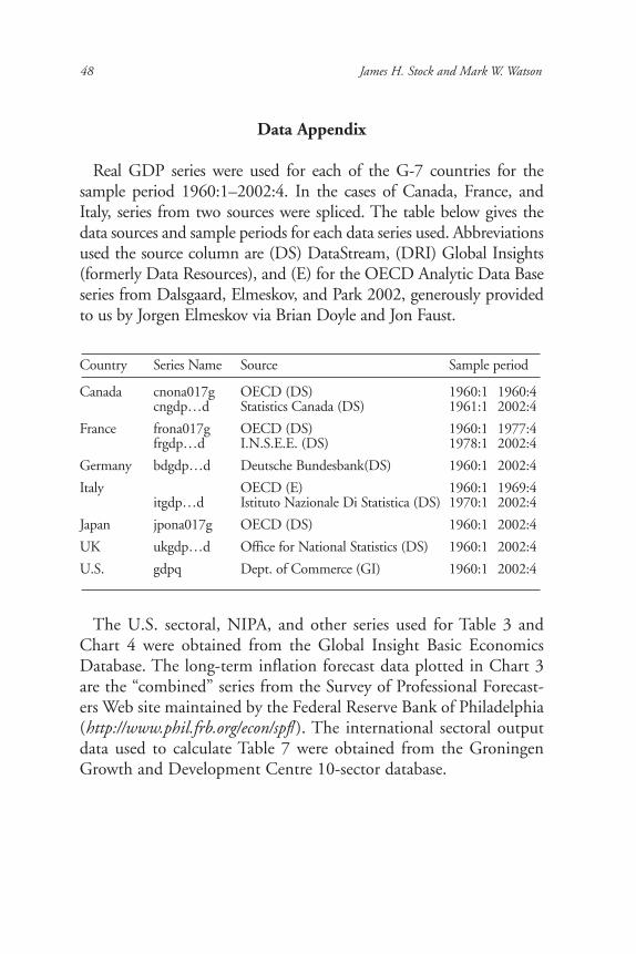
Real GDP series were used for each of the G-7 countries for thesample period 1960:1–2002:4. In the cases of Canada, France, andItaly, series from two sources were spliced. The table below gives thedata sources and sample periods for each data series used. Abbreviationsused the source column are (DS) DataStream, (DRI) Global Insights(formerly Data Resources), and (E) for the OECD Analytic Data Baseseries from Dalsgaard, Elmeskov, and Park 2002, generously providedto us by Jorgen Elmeskov via Brian Doyle and Jon Faust.
The U.S. sectoral, NIPA, and other series used for Table 3 andChart 4 were obtained from the Global Insight Basic EconomicsDatabase. The long-term inflation forecast data plotted in Chart 3are the “combined” series from the Survey of Professional Forecast-ers Web site maintained by the Federal Reserve Bank of Philadelphia(http://www.phil.frb.org/econ/spf/). The international sectoral outputdata used to calculate Table 7 were obtained from the GroningenGrowth and Development Centre 10-sector database.
France frona017g OECD (DS) 1960:1 1977:4frgdp…d I.N.S.E.E. (DS) 1978:1 2002:4
Germany bdgdp…d Deutsche Bundesbank(DS) 1960:1 2002:4
Italy OECD (E) 1960:1 1969:4itgdp…d Istituto Nazionale Di Statistica (DS) 1970:1 2002:4
Japan jpona017g OECD (DS) 1960:1 2002:4
UK ukgdp…d Office for National Statistics (DS) 1960:1 2002:4
U.S. gdpq Dept. of Commerce (GI) 1960:1 2002:4
Endnotes1Taylor 1979 presents a graph like our Figure 1 with the frontier and point A
estimated empirically.
2The literature on the great moderation has grown rapidly. Blanchard and Simon2001 and Stock and Watson 2002 survey studies using U.S. data. Studies using inter-national data include Dalsgaard, Elmeskov, and Park 2002; Del Negro and Otrok2003; Doyle and Faust 2002a; van Dijk, Osborn, and Sensier 2002; Fritsche andKouzine 2003; Mills and Wang 2000; Simon 2001; and Stock and Watson 2003.
3The estimates in Chart 2 are taken from Stock and Watson 2003. Theinstantaneous standard deviation is computed by first estimating a stochasticvolatility autoregressive model with time varying parameters, specifically, yt = α0t + ∑ p
t = 1nσ 2t-1 + ζt , εt , η1t ,..., ηpt are i.i.d. N(0,1), and ζt is drawn from a
mixture-of-normals distribution and is distributed independently of the othershocks. Next, the instantaneous variance of four-quarter GDP growth iscomputed as a function of the smoothed estimates of the time-varying param-eters. For details, see Stock and Watson 2002, Appendix A, and Stock andWatson 2003.
4This reasoning assumes the long-term growth rate to be approximately constant.This is not a good assumption for Germany, Italy, and Japan, where the long-termmean growth rate fell substantially. In the presence of a constant variance, this fallwould increase recession lengths and decrease expansion lengths. Accordingly, theimplications of the great moderation for business cycle phase lengths for thosecountries require model-based calculations, such as those in Harding and Pagan2002. See Blanchard and Simon 2001 for additional discussion.
5Repeating this exercise for forecasts of four-quarter GDP growth shows a similarreduction in pseudo out-of-sample forecast root mean squared errors. These calcu-lations are based on the fully revised data, which were not available to real-timeforecasts, so a real-time forecaster might not have realized the forecast improve-ments apparent in Table 2.
6See Dalsgaard, Elmeskov, and Park 2002; Doyle and Faust 2002a, 2002b;Heathcoate and Perri 2002; Kose, Prasad, and Terrones 2003; Monfort, Renne, andVitale 2002; and Stock and Watson 2003. Some researchers have suggested theemergence of a euro zone business cycle (Artis, Kontelemis, and Osborn 1997);Artis and Zhang 1997, 1999; Carvalho and Harvey 2002; Helbling and Bayoumi2003; Dalsgaard, Elmeskov, and Park 2002; Del Negro and Otrok 2003; Lugin-buhl and Koopman 2003; however, the time period available to assess thispossibility is short, so it is difficult to draw clear statistical conclusions and we donot pursue this finding here.
Has the Business Cycle Changed? Evidence and Explanations 49
7For accounts of these institutional and policy changes in the United States, seeDeLong 1997, Romer and Romer 2002, Sargent 1999; for an international perspec-tive, see Bernanke and Mishkin 1992 and Bernanke and others 1999.
8In practice, monetary policy necessarily involves discretion and considersmany variables, not just the rate of inflation and the output gap; strictly, none ofthis is permitted under the Taylor rule (1). Moreover, the Taylor rule is difficultto implement in real time because of the large uncertainty about the level ofpotential output (e.g., Kohn 1999). Our immediate purpose is not, however, todispense policy advice. Rather, it is to quantify the key broad features of mone-tary policy over the past 30 years, a job for which the Taylor rule provides a usefulmodeling simplification.
9Other studies that find that U.S. monetary policy became more aggressive after1979 include Boivin and Giannoni 2002, and Cogley and Sargent 2001, 2002. Inter-estingly, based on an analysis of real-time data, Orphanides 2001, 2002 suggests thatthis change might not reflect a shift in the preferences of the policymakers, whoalways intended to respond aggressively to inflation, but rather flaws in their estimatesof potential GDP, which failed to detect the productivity slowdown of the early1970s. Under Orphanides’ story, policymakers in the 1970s thought they were beingmore aggressive than they actually were. The large institutional shifts of the hardERM period and the transition to monetary union, with their short sample periods,make it difficult to quantify shifts in policy in Europe, although Clarida, Gali, andGertler 1998 provide some evidence.
10The RS and SVAR base models, including their base policy rules, were esti-mated using post-1984 data (we re-estimated the RS and SVAR models using theoriginal specifications and data from 1984 to 2002). The SW-US and SW-EU basemodels were estimated by the original authors using a single full sample, in the U.S.case 1957-2002 and in the EU case 1980-1999; the original SW estimated policyrule coefficients are very close to the Taylor coefficients of 1.5 and 0.5 and thusreflect post-1984 policy.
11The results are available in the Technical Appendix.
12We thank Refet Gürkaynak, Brian Sack, and Eric Swanson for bringing thesedata to our attention.
13The data are annual growth rates, taken from the Groningen Growth andDevelopment Centre 10-sector database. The 10 sectors are agriculture, mining,manufacturing, construction, public utilities, retail and wholesale trade, transportand communication, finance and business services, other market services, andgovernment services. The German data are for West Germany only.
50 James H. Stock and Mark W. Watson
14Another explanation could be changes in the way these series are collected,which induce the changing volatilities observed in Chart 4; see Edge 2000 for adiscussion of these data. However, the decline in volatility is evident in other meas-ures of residential construction activity, including building permits, housing starts,and purchases of residential structures.
15The only panel data set on individual-level consumption is the Panel Survey onIncome Dynamics (PSID), which only records food consumption. Blundell andothers 2003 make their inferences about overall consumption volatility by usingeconometric models of consumption to combine data from the PSID and from theConsumer Expenditure Survey, a sequence of detailed cross-sectional surveys ofconsumption. Blundell and Preston 1998 report evidence for the UK of an increasein the variance of micro-level consumption.
16Smets and Wouters 2003a, 2003b estimated their models over a single sampleperiod, so for SW-US and SW-EU we do not have estimates of pre-1979 shockvariances in those models. In addition, it is not clear how sensible it is to calibratethe SW-EU model to first-period U.S. shocks (how would Europe have respondedto U.S. shocks?).
17The extent of the decline in the standard deviation of productivity shocks, andperhaps even whether there was such a decline, depends on the measure of produc-tivity shocks used. Measuring the volatility reduction using other measures ofproductivity shocks and reconciling the results merits further research.
18For additional discussion, see Doyle and Faust 2002a and Heathcoate andPerri 2002.
19Systems like (2) contain more shocks than observable variables; with seven coun-tries and one common shock, there are eight shocks. Estimation of these systemsrequires factor model methods. Stock and Watson 2003 estimate a seven equationversion of (2) with additional lag restrictions. Monfort, Renne, and Vitale 2002model the international linkages as arising entirely from current and lagged effects ofthe common international shocks, while Helbling and Bayoumi 2003 make a similarassumption, but estimate the system using nonparametric methods.
Has the Business Cycle Changed? Evidence and Explanations 51
52 James H. Stock and Mark W. Watson
References
Ahmed, Shagil, Andrew Levin, and Beth Wilson. “Recent U.S. MacroeconomicStability: Good Luck, Good Policies, or Good Practices?” manuscript, 2001,Board of Governors of the Federal Reserve System.
Albanesi, Stefania, V.V. Chari, and Lawrence J. Christiano. “Expectation Traps andMonetary Policy,” Review of Economic Studies, forthcoming 2003.
Artis, Michael J., Zenon G. Kontolemis, and Denise R. Osborn. “Business Cyclesfor G-7 and European Countries,” Journal of Business 70, 1997, pp. 249-279.
Artis, Michael J., and Wenda Zhang. “International Business Cycles and the ERM:Is There a European Business Cycle?” International Journal of Finance andEconomics 2, 1997, pp. 1-16.
_______, and _______. “Further Evidence on the International Business Cycle andthe ERM: Is there a European Business Cycle?” Oxford Economic Papers 51, 1999,pp. 120-132.
Bernanke, Ben S., and Frederic Mishkin. “Central Bank Behavior and the Strategyof Monetary Policy: Observations from Six Industrialized Countries,” NBERMacroeconomics Annual 7, 1992, pp. 183-228.
Bernanke, Ben S., and Ilian Mihov. “Measuring Monetary Policy,” QuarterlyJournal of Economics, 1998, pp. 869-902.
Bernanke, Ben S., Thomas Laubach, Frederic S. Mishkin, and Adam S. Posen.Inflation Targeting, Lessons from the International Experience, Princeton, N.J.:Princeton University Press, 1999.
Blanchard, Olivier, and John Simon. “The Long and Large Decline in U.S. OutputVolatility,” Brookings Papers on Economic Activity 1, 2001, pp. 135-164.
Blundell, Richard, and Ian Preston. “Consumption Inequality and Income Uncer-tainty,” Quarterly Journal of Economics 113, 1998, pp. 603-640.
Blundell, Richard, Luigi Pistaferri, and Ian Preston. “Consumption Inequality andPartial Insurance,” manuscript, 2003, University College London.
Boivin, Jean, and Marc Giannoni. “Has Monetary Policy Become Less Powerful?”manuscript, 2002, Columbia University.
Buch, Claudia M., Joerg Doepke, and Christian Pierdzioch.“Financial Opennessand Business Cycle Volatility,”Journal of International Money and Finance, forth-coming 2003.
Has the Business Cycle Changed? Evidence and Explanations 53
Burns, Arthur. “Progress Towards Economic Stability,” American Economic Review50(1), 1960, pp. 2-19.
Campbell, John Y., Martin Lettau, Burton G. Malkiel, and Yexiao Xu. “Have Indi-vidual Stocks Become More Volatile? An Empirical Exploration of IdiosyncraticRisk,” The Journal of Finance 56(1), 2001.
Carvalho, Vasco M., and Andrew C. Harvey. “Convergence and Cycles in the Euro-Zone,” manuscript, 2002, University of Cambridge.
Christiano, Lawrence J., Martin Eichenbaum, and Charles L. Evans. “MonetaryPolicy Shocks: What Have We Learned and To What End?” Handbook of Macro-economics 1, 1999, pp. 65-148.
Clarida, Richard, Jordi Gali, and Mark Gertler. “Monetary Policy Rules in Practice:Some International Evidence,” European Economic Review 42, 1998, pp. 1033-1067.
_______, _______, and _______. “Monetary Policy Rules and MacroeconomicStability: Evidence and Some Theory,” Quarterly Journal of Economics 115, 2000,pp. 147-180.
Cogley, Timothy, and Thomas J. Sargent. “Evolving Post-World War II U.S. Infla-tion Dynamics,” NBER Macroeconomics Annual 16, 2001, pp. 331-373.
_______, and _______. “Drifts and Volatilities: Monetary Policies and Outcomesin the Post WWII U.S.,” manuscript, 2002, Stanford University.
Comin, Diego, and Sunil Mulani. “Diverging Trends in Macro and Micro Volatil-ity: Facts,” manuscript, 2003, New York University.
Dalsgaard, Thomas, Jorgen Elmeskov, and Cyn-Young Park. “Ongoing Changes inthe Business Cycle—Evidence and Causes,” OECD Economics Departmentworking paper no. 315, 2002.
Del Negro, Marco, and Christopher Otrok. “Time-Varying European BusinessCycles,” manuscript, 2003, University of Virginia.
DeLong, J. Bradford. “America’s Peacetime Inflation: The 1970s,” in Christina D.Romer and David H. Romer, eds., Reducing Inflation: Motivation and Strategy,Chicago: University of Chicago Press, 1997, pp. 147-176.
van Dijk, Dick, Denise R. Osborn, and Marianne Sensier. “Changes in the Vari-ability of the Business Cycle in the G-7 Countries,” manuscript, 2002, ErasmusUniversity Rotterdam.
Doyle, Brian M., and Jon Faust. “An Investigation of Co-Movements among theGrowth Rates of the G-7 Countries,” Federal Reserve Bulletin, October 2002a,pp. 427-437.
_______, and _______. “Breaks in the Variability and Co-Movement of G-7Economic Growth,” manuscript, 2002b, Federal Reserve Board.
Easterly, William, R. Islam, and Joseph E. Stiglitz. “Shaken and Stirred: ExplainingGrowth Volatility,” in B. Pleskovic, ed., Annual World Bank Conference on Devel-opment Economics, 2001, pp. 191-211.
Edge, Rochelle M. “The Effect of Monetary Policy on Residential and StructuresInvestment under Differential Project Planning and Completion Times,” Inter-national Finance discussion paper no. 671, Board of Governors of the FederalReserve System, 2000.
Fritsche, Ulrich, and Vladimir Kouzine. “Declining Output Volatility and Mone-tary Policy in Germany,” manuscript, 2003, German Institute for EconomicResearch (DIW Berlin).
Gürkaynak, Refet S., Brian Sack, and Eric Swanson. “The Excess Sensitivity ofLong-Term Interest Rates: Evidence and Implications for MacroeconomicModels,” manuscript, 2003, Division of Monetary Affairs, Board of Governorsof the Federal Reserve System.
Hamilton, James D. “This Is What Happened to the Oil Price-MacroeconomyRelationship,” Journal of Monetary Economics 38(2), 1996, pp. 215-220.
_______. “What Is an Oil Shock?” Journal of Econometrics 113, 2003, pp. 363-398.
Harding, Don, and Adrian Pagan. “Dissecting the Cycle: A Methodological Inves-tigation,” Journal of Monetary Economics 49, 2002, pp. 365-381.
Heathcoate, Jonathan, and Fabrizio Perri. “Financial Globalization and RealRegionalization,” NBER working paper 9292, 2002.
Helbling, Thomas, and Tamim Bayoumi. “Are They All in the Same Boat? The2000-2001 Growth Slowdown and the G-7 Business Cycle Linkages,” manu-script, 2003, International Monetary Fund.
Hooker, Mark A. “What Happened to the Oil Price-Macroeconomy Relationship?”Journal of Monetary Economics 28, 1996, pp. 195-213.
Judd, John F., and Glenn D. Rudebusch. “Taylor’s Rule and the Fed: 1970-1997,”Federal Reserve Bank of San Francisco Economic Review 3, 1998, pp. 3-16.
Kahn, James, Margaret M. McConnell, and Gabriel Perez-Quiros. “On the Causesof the Increased Stability of the U.S. Economy,” Federal Reserve Bank of NewYork Economic Policy Review 8(1), 2002, pp. 183-202.
Kim, Chang-Jin, and Charles R. Nelson. “Has the U.S. Economy Become MoreStable? A Bayesian Approach Based on a Markov-Switching Model of the Busi-ness Cycle,” The Review of Economics and Statistics 81, 1999, pp. 608-616.
54 James H. Stock and Mark W. Watson
Kohn, Donald L. “Comment on ‘Forward-Looking Rules for Monetary Policy’,” inJohn B. Taylor, ed., Monetary Policy Rules, Chicago: University of Chicago Press,1999, pp. 192-199.
Kose, M. Ayhan, Eswar S. Prasad, and Marco E. Terrones. “How Does GlobalizationAffect the Synchronization of Business Cycles?” IZA Discussion Paper no. 702, 2003.
Kozicki, Sharon, and Peter A. Tinsley. “Shifting Endpoints in the Term Structure ofInterest Rates,” Journal of Monetary Economics 47, 2001, pp. 613-652.
Luginbuhl, Rob, and Siem Jan Koopman. “Convergence in European GDP Series:A Multivariate Common Converging Trend-Cycle Decomposition,” TinbergenInstitute discussion paper 2003-031/4, 2003.
Maccini, Lou, and Adrian Pagan. “Exploring the Role of Inventories in the Busi-ness Cycle,” manuscript, 2003.
McCarthy, Jonathan, and Richard W. Peach. “Monetary Policy Transmission toResidential Investment,” Federal Reserve Bank of New York Economic PolicyReview 8(1), 2002, pp. 139-158.
McConnell, Margaret M, and Gabriel Perez-Quiros. “Output Fluctuations in theUnited States: What Has Changed Since the Early 1980s,” American EconomicReview 90(5), 2000, pp. 1464-1476.
Mills, Terence C., and Ping Wang. “Searching for the Sources of Stabilisation inOutput Growth Rates: Evidence from the G-7 Economies,” manuscript, 2000.
Moffitt, Robert A., and Peter Gottschalk. “Trends in the Transitory Variance ofEarnings in the United States,” The Economic Journal 112, 2002, pp. C68-C73.
Monfort, A., J.P. Renne, R. Rüffer, and G. Vitale. “Is Economic Activity in the G-7 Synchronized? Common Shocks vs. Spillover Effects,” manuscript, 2002.
Moore, Geoffrey H., and Victor Zarnowitz. "The Development and Role of theNBER's Business Cycle Chronologies," in Robert J. Gordon (ed.), The AmericanBusiness Cycle: Continuity and Change. Chicago: University of Chicago Press, 1986.
Nordhaus, William D. “Productivity Growth and the New Economy” (with discus-sion), Brookings Papers on Economic Activity 2002(2), pp. 211-265.
Orphanides, Athanasios. “Monetary Policy Rules Based on Real-Time Data,”American Economic Review 91(4), 2001, pp. 964-985.
__________. “Monetary Policy Evaluation with Noisy Information,” Journal ofMonetary Economics 50(3), 2003, pp. 605-631.
Ramey, Valerie A., and Daniel J. Vine. “Tracking the Source of the Decline in GDPVolatility: An Analysis of the Automobile Industry,” manuscript, 2003.
Has the Business Cycle Changed? Evidence and Explanations 55
Romer, Christina D., and David H. Romer. “The Evolution of Economic Under-standing and Postwar Stabilization Policy,” Rethinking Stabilization Policy,Federal Reserve Bank of Kansas City, 2002, pp. 11-78.
Rudebusch, Glenn, and Lars E.O. Svensson. “Policy Rules for Inflation Targeting,”in John B. Taylor, ed., Monetary Policy Rules, University of Chicago Press,Chicago, 1999, pp. 203-246.
Sargent, Thomas J. The Conquest of American Inflation, Princeton: PrincetonUniversity Press, 1999.
Sensier, Marianne, and Dick van Dijk, “Short-Term Volatility Versus Long-TermGrowth: Evidence in U.S. Macroeconomic Time Series,” manuscript, 2001,University of Manchester.
Simon, John. “The Decline in Australian Output Volatility,” manuscript, 2001,Reserve Bank of Australia.
Smets, Frank, and Raf Wouters. “An Estimated Dynamic Stochastic General Equi-librium Model of the Euro Area,” Journal of the European Economic Association,forthcoming 2003a.
_______, and _______. “Shocks and Frictions in U.S. Business Cycles: A BayesianDSGE Approach,” manuscript, 2003b.
Staiger, Douglas, James H. Stock, and Mark W. Watson. “Prices, Wages and the U.S.NAIRU in the 1990s,” chapter 1 in The Roaring Nineties, A. Krueger and R. Solow,eds., Russell Sage Foundation/The Century Fund: New York, 2001, pp. 3-60.
Stock, James H., and Mark W. Watson. “Has the Business Cycle Changed andWhy?” NBER Macroeconomics Annual, 2002, pp. 159-218.
_______, and _______. “Understanding Changes in International Business CycleDynamics,” manuscript, 2003.
Taylor, John B. “Estimation and Control of a Macroeconomic Model with RationalExpectations,” Econometrica 47, 1979, pp. 1267-1286.
_______. “Discretion Versus Policy Rules in Practice,” Carnegie-Rochester Confer-ence Series on Public Policy 39, 1993, pp. 195-214.
_______. “A Historical Analysis of Monetary Policy Rules,” in John B. Taylor (ed.),Monetary Policy Rules, Chicago: University of Chicago Press, 1999, pp. 319-340.
Watson, Mark W. “Explaining the Increased Variability in the Long-Term Inter-est Rate,” Federal Reserve Bank of Richmond Economic Quarterly 85, 1999.