The undersigned certify that they have read, and recommend to the Faculty of Graduate
Studies for acceptance, a thesis entitled "Mathematical Modeling of Convective Mixing
in Porous Media for Geological CO2 Storage" submitted by Hassan Hassanzadeh in
partial fulfilment of the requirements of the degree of Doctor of Philosophy.
________________________________
Supervisor Dr. Mehran Pooladi-Darvish Department of Chemical and Petroleum Engineering _______________________________
Co-Supervisor Dr. David W. Keith Department of Chemical and Petroleum Engineering ________________________________
Dr. Abdulmajeed A. Mohamad Department of Mechanical and Manufacturing Engineering ________________________________
Dr. Antonin (Tony) Settari Department of Chemical and Petroleum Engineering ________________________________
Dr. Les Sudak Department of Mechanical and Manufacturing Engineering ________________________________
External Examiner
Dr. Ben Rostron Department of Earth & Atmospheric Science University of Alberta _______________ Date
iv
Abstract
As concern about the adverse consequences of anthropogenic climate change has grown,
so too has research into methods to reduce the emissions of greenhouse gases that will
drive future climatic change. Carbon dioxide emissions arising from use of fossil-fuels
are likely to be the dominant drivers of climate change over the coming century. The use
of carbon dioxide and geologic storage (or sequestration) offers the possibility of
maintaining access to fossil energy while reducing emissions of carbon dioxide to the
atmosphere. One of the essential concerns in geologic storage is the risk of leakage of
CO2 from the injection sites. Carbon dioxide injected into saline aquifers, dissolves in the
resident brines, increasing their density potentially leading to convective mixing.
Convective mixing increases the rate of dissolution, and therefore decreases the time-
scale over which leakage is possible. Understanding the factors that drive convective
mixing and accurate estimation of the rate of dissolution in saline aquifers is important
for assessing geological CO2 storage sites.
This dissertation has three components, which includes linear stability analysis,
prediction of CO2-brine PVT, and numerical modeling. A hydrodynamic stability
analysis is performed for non-linear, transient concentration fields in a saturated,
homogenous and isotropic porous medium under various initial and boundary conditions.
The role of the natural flow of aquifers and associated dispersion on the onset of
convection in the saline aquifers is also investigated. A fugacity and an activity models
are combined to develop an accurate thermodynamic module appropriate for geological
CO2 storage application. A three-dimensional, two-phase and two-component numerical
model for simulation of CO2 storage in saline aquifers is also developed. The numerical
model employs higher order and total-variation-diminishing schemes, capillary pressure,
relative permeability hysteresis, and full dispersion tensor formulation. The model also
takes into account an accurate representation of a CO2-brine mixture thermodynamic and
transport properties. The model is validated for a number of problems against one- and
two-dimensional standard analytical and numerical solutions.
v
The theoretical analysis and numerical model are used to investigate the role of
convective mixing on CO2 storage in homogenous and isotropic saline aquifers. Scaling
analysis of the convective mixing of CO2 in saline aquifers is presented. The convective
mixing of CO2 in aquifers is characterized, and three mixing periods are identified. It is
found that mixing achieved can be approximated by a scaling relationship for Sherwood
number as a measure of mixing. Furthermore, the onset of natural convection and the
wavelengths of the initial convective instabilities are determined. A criterion is also
developed that provides the appropriate numerical mesh resolution required for accurate
modeling of convective mixing of CO2 in deep saline aquifers. In addition, using the
model developed, a method to accelerate CO2 dissolution in brines is also suggested. The
acceleration of dissolution by brine pumping increases the rate of solubility trapping in
saline aquifers and therefore increases the security of storage. Results of this dissertation
give insight into appropriate implementation of large scale geological CO2 storage in
deep saline aquifers.
vi
Acknowledgements
Many people have aided in the initiation, progress and achievement of this study, each in
their own way. Without their help this work would not be possible. First, I would like to
express my sincere appreciation to my advisor Dr. Mehran Pooladi-Darvish and my co-
advisor Dr. David W. Keith for their outstanding knowledge, supervision,
encouragements, insight, and patience during my research at the University of Calgary.
They have been a continuous source of enthusiasm and support for this research. I am
especially grateful to Mehran for giving me the opportunity to learn and grow under his
guidance, and for always giving me enough independence to pursue my own thoughts.
My gratitude also extends to Dr. Abdulmajeed A. Mohamad for serving on my
dissertation committee and also Dr. Tony Settari, Dr. Les Sudak, Dr. Ben Rostron and Dr.
Jocelyn Grozic for serving on my examining committee. I must again acknowledge Dr.
Tony Settari who has supported this work significantly. I am also thankful to Dr. Ali
Mohammad Saidi for many valuable discussions on convection and diffusion. I would
also like to thank Dr. Ayodeji A. Jeje for the technical discussions we enjoyed during the
Advance Heat Transfer & Fluid Dynamics and Macro Transport courses.
I would also like to thank my friends and fellow graduate students, Hussain Sheikha,
Shahab Gerami, Majid Saeedi, Amir Shahbazi, and Mohammad Shahvali from
Fundamental Research in Reservoir Modeling (FRRM), for their constant support,
friendship and discussions during my years at the University of Calgary, which made the
research group an enjoyable and creative environment to work in. My gratitude also goes
to the National Iranian Oil Company (NIOC) for providing me with a scholarship. The
financial support for this work was provided by the National Science and Engineering
Research Council of Canada (NSERC) and by the Alberta Department of Energy. This
support is gratefully acknowledged.
Lastly, and most importantly, I have to thank my wife, Marzieh, our parents, my daughter
Fatemeh and my son Ehsan for the love, encouragement, care, and support they have
given me all the way.
vii
Dedication
To my parents, my wife Marzieh, my daughter Fatemeh and my son Ehsan
viii
Table of Contents
Approval Page..................................................................................................................... ii Abstract .............................................................................................................................. iv Acknowledgements............................................................................................................ vi Table of Contents............................................................................................................. viii List of Tables ..................................................................................................................... xi List of Figures .................................................................................................................. xiii Nomenclature.................................................................................................................. xxii
CHAPTER ONE: INTRODUCTION..................................................................................1 1.1 Background................................................................................................................1 1.2 Solubility trapping .....................................................................................................2 1.3 Residual phase trapping .............................................................................................3 1.4 Mineral trapping ........................................................................................................3 1.5 Motivations and objectives ........................................................................................4 1.6 Components and outline of the study ........................................................................5
1.6.1 Linear stability analysis ......................................................................................6 1.6.2 Prediction of CO2-brine mixture PVT and transport properties .........................7 1.6.3 Development, testing and application of a numerical model..............................7
CHAPTER TWO: LITERATURE REVIEW......................................................................9 2.1 Introduction................................................................................................................9 2.2 Literature on geological CO2 sequestration ...............................................................9
2.2.1 Examples of CO2 storage in geological formations around the world..............14 2.3 Literature on density-driven flow ............................................................................17 2.4 Concluding remarks.................................................................................................21
CHAPTER THREE: STABILITY OF A FLUID IN A HORIZONTAL SATURATED POROUS LAYER .............................................................................................................23
3.1 Introduction..............................................................................................................23 3.2 Formulation of flow and transport equations...........................................................24
3.2.1 Base state ..........................................................................................................25 3.2.2 The perturbation equations ...............................................................................26
3.4 Stability analysis of classical problem of Horton-Rogers-Lapwood .......................28 3.4.1 Amplitude equations .........................................................................................30
3.5 Effect of non-linear concentration profile, initial, and boundary conditions...........34 3.5.1 Case 1: Step change at the top and closed at the bottom ..................................36 3.5.2 Case 2: Step change at the top and zero concentration at the bottom...............39 3.5.3 Case 3: Ramp contact........................................................................................40
3.6 Solution Methodology .............................................................................................42 3.7 Results and discussion .............................................................................................44 3.8 Applications for geological CO2 storage-I...............................................................49
ix
3.9 The effect of dispersion on the onset of buoyancy-driven convection ....................51 3.9.1 Model Description ............................................................................................52
3.10 Results and Discussion ..........................................................................................58 3.11 Applications for geological CO2 storage-II ...........................................................64 3.12 Effect of geothermal gradient ................................................................................66 3.13 Concluding remarks...............................................................................................68
CHAPTER FOUR: PREDICTING PVT DATA OF A CO2-BRINE MIXTURE.............71 4.1 Introduction..............................................................................................................71 4.2 Review .....................................................................................................................73 4.3 Thermodynamic model ............................................................................................74
4.3.1 Density of the aqueous phase............................................................................79 4.4 Comparison of module predictions with experimental data and published correlations: ...................................................................................................................80
4.4.1 Comparison with experimental data .................................................................80 4.4.2 Comparison with other predictive tools ............................................................85
4.5 Transport properties of the CO2/Water system........................................................88 4.5.1 Brine viscosity ..................................................................................................88 4.5.2 Gas phase viscosity ...........................................................................................90 4.5.3 Molecular diffusion coefficient: .......................................................................91
4.6 Application for representation of CO2-brine PVT data for a black oil flow simulator ........................................................................................................................92 4.7 Concluding remarks.................................................................................................94
CHAPTER FIVE: MATHEMATICAL MODEL DESCRIPTION AND TESTING .......96 5.1 Introduction..............................................................................................................96 5.2 The Governing Equations ........................................................................................97 5.3 Numerical representation of the IMPES formulation ............................................100
5.4 Dispersion flux and dispersion coefficients...........................................................105 5.5 Approximation of convective terms ......................................................................109
5.5.1 Single-point upstream .....................................................................................109 5.5.2 Two-point upstream ........................................................................................110 5.5.3 Third order methods........................................................................................111 5.5.4 Total Variation diminishing methods (TVD) .................................................113
5.6 Relative permeability hysteresis ............................................................................115 5.7 Well model.............................................................................................................117 5.8 Model testing .........................................................................................................119 5.9 Pressure diffusivity ................................................................................................120 5.10 Mass diffusivity ...................................................................................................126 5.11 Convection-diffusion ...........................................................................................131 5.12 Hydrostatic test problem......................................................................................136 5.13 Horton-Rogers-Lapwood (HRL) instability problem..........................................138 5.14 Elder problem ......................................................................................................141
x
5.15 The Henry sea water intrusion .............................................................................144 5.16 Buckley Leverett problem ...................................................................................147 5.17 Countercurrent imbibition in a water-wet matrix block ......................................149 5.18 Summary..............................................................................................................152
CHAPTER SIX: APPLICATIONS .................................................................................154 6.1 Introduction............................................................................................................154 6.2 Convective mixing in an isotropic and homogenous saturated porous medium ...155
6.2.1 Description of the problem .............................................................................155 6.2.2 Numerical analysis..........................................................................................157 6.2.3 Mixing mechanisms ........................................................................................158
6.3 Scaling analysis......................................................................................................164 6.3.1 Onset of natural convection ............................................................................164 6.3.2 Initial wavelength of the convection instabilities ...........................................165 6.3.3 Mixing periods and total mixing.....................................................................167
6.4 Speculation concerning the role of heterogeneity..................................................170 6.5 Discussion..............................................................................................................171 6.6 Boussinesq approximation.....................................................................................174 6.7 Simulation of CO2 storage in saline aquifers.........................................................175
6.7.1 Drying effect ...................................................................................................181 6.7.2 Acceleration of CO2 dissolution in saline aquifers .........................................182
6.8 Summary and conclusions .....................................................................................186
CHAPTER SEVEN: CONCLUSIONS AND RECOMMENDATIONS........................189 7.1 Conclusions............................................................................................................189
7.1.1 Theoretical analysis ........................................................................................189 7.1.2 Numerical model and its applications.............................................................191 7.1.3 Accurate representation of a CO2 and brine mixture ......................................192
7.2 Recommendations for future research ...................................................................193 7.2.1 Stability analysis and convective mixing under two-phase flow condition....193 7.2.2 Role of heterogeneity structure on instability .................................................193 7.2.3 The effect of dispersion on convective mixing...............................................193 7.2.4 Investigation of non-Darcy flow effect on the onset of convection................194 7.2.5 Dissolution acceleration..................................................................................194
APPENDIX......................................................................................................................213 Summary of scaling relationships................................................................................213
xi
List of Tables
Table 2.1: World wide projects related to Carbon Dioxide geologic storage (IPCC Report,
Figure 6.21: The effect of water injection on the fraction of CO2 dissolved in formation
water as compared to a case without water injection.............................................. 186
xxii
Nomenclature
A time components of the perturbed velocity amplitude function a dimensionless wavenumber a equation of state parameter a activity B time components of the perturbed concentration amplitude function Bw water formation volume factor b equation of state parameter C concentration CR grid courant number
LandC land trapping constant c fraction of ultimate dissolution cw water compressibility c amplification factor D molecular diffusion D derivative operator F formation resistivity factor d derivative g gravitational acceleration H porous layer thickness I ionic strength I integral function i imaginary number Jlk diffusive flux of component k in phase l K equilibrium constants Krr
dispersion tensor k permeability krg gas relative permeability krw water relative permeability k constant 12103805.1 −×= LR reference length Mk mass of each component k in a grid block Mw molecular weight m molality mt total mass n mole nz number of layers p pressure pc capillary pressure Pc critical pressure Par parameter, it can be either ξ or ζ PE grid Peclet number
xxiii
Pe peclet number PVT pressure-volume-temperature Q sink or source for a phase q sink or source for a component R gas constant Ra rayleigh number RaG grid block Rayleigh number Rs solubility of CO2 in brine gas r radius of the molecule S salt content in mass fraction S saturation Sgc critical gas saturation Sh Sherwood number s skin factor Sgtrap trapped gas saturation T temperature Tc critical temperature T grid block transmissibility t time tc time to onset of convection TVD total variation diminishing V volume
iV average partial molar volume of the pure component i Vφ apparent molar volume v vector of Darcy velocity xi mole fraction of component i in liquid phase x length in x-direction yi mole fraction of component i in gas phase y length in y-direction z length in z-direction zi global mole fraction of component i zi valence of each species present in a solution αD decline factor for ramp boundary condition αL longitudinal dispersivity αT transverse dispersivity αt thermal diffusivity β coefficient of density increase δ kronecker delta δD dimensionless diffusion penetration depth ∆ increment of a variable, for example ∆x
2COγ the activity coefficient of the dissolved CO2
xxiv
ρ density Г components dispersive transmisibilities τ tortuosity θ limiting function in TVD method φ fugacity coefficient Φ association factor of the liquid Λ weighting factors to account for variable mesh size Ω weighting factor used in finite difference formulation υ density coupling ω mass fraction of CO2 in brine ω time amplification of perturbations ξ second-order interaction parameters λ wavelength of the convective instabilities λl mobility of phase l λp the pore size distribution index ζ third-order interaction parameters κ equilibrium ratio µ viscosity σ constant depends on the exterior boundary of the grid block in well model Subscripts 0 base state 1 solvent 2 solute A anion α aqueous b brine C cation CO2 carbon dioxide D dimensionless g gas H2O water L longitudinal l integral or summation index i component index k component index l phase l m grid block index m integral or summation index
xxv
max maximum mix mixture L liquid n summation index r relative or reference res reservoir condition sc standard condition w water x x-coordinate direction y y-coordinate direction z z-coordinate direction Superscripts 0 end point of the relative permeability curves c convective ° reference state n time step index s equilibrium state ‘ perturbed state * amplitude of the perturbations
1
CHAPTER ONE: INTRODUCTION
1.1 Background
Concentration of CO2 in the atmosphere has been steadily increasing from 280 ppmv
since the industrial revolution to recent level of 380 ppmv due to fossil energy
consumption (Houghton et al., 2001). Emissions of CO2 from fossil-fuel in the year of
2000 are estimated to be 23.5 Gt/yr or approximately 6 Gt/yr of carbon (IPCC, 2005).
The CO2 concentration may continue to increase to between 500 and 1000 ppmv by the
year of 2100 (Houghton et al., 2001). Greenhouse gases absorb the radiated heat from
the Earth and reradiate it back to the Earth through the natural greenhouse gas system.
Excessive atmospheric CO2 concentration enhances the natural greenhouse effect and
warms the planet. Global warming will have severe impacts on the environment and on
society (Trenberth, 1997). If the Earth continues to warm it is predicted that the
temperature at the Earth's surface may increase 1.4 to 5.8 °C by 2100 (Houghton et al.,
2001). Higher temperatures will cause a melting of ice in the Arctic and Antarctic
regions. This will speed up the rise of sea level. To avoid large climate change emissions
will need to be reduced to nearly zero over 21st century.
Marchetti (1977) proposed that the climatic impact of fossil fuel can be reduced by
separating the resulting carbon and sequestering it away from the atmosphere. One way
of reducing the atmospheric CO2 level is subsurface storage of CO2. The use of
technologies to capture and store CO2 is rapidly emerging as a potentially important tool
for managing carbon emissions (Bachu and Adams, 2003). Geological storage, defined as
the process of injecting CO2 into geologic formations for the explicit purpose of avoiding
atmospheric emission of CO2, is perhaps the most important near term option. Geological
storage promises to reduce the cost of achieving deep reductions in CO2 emissions over
the next few decades. At least three alternatives are available for geological CO2 storage.
These include: depleted oil and gas fields (global capacity ~ 200-500 GtC), deep coal
beds (~ 100-200 GtC), and deep saline aquifers (~ 102-103 GtC) (Keith, 2002). Deep
2
saline aquifers are a particularly important class of geologic storage system because of
their ubiquity and large capacity. Several mechanisms are involved in the storage process.
In a typical CO2 storage some of the injected CO2 dissolves in the formation water
(solubility trapping) (Bachu and Adams, 2003), some may be trapped as residual gas
saturation (residual gas trapping) (Felett et al., 2004), and some may react with host
minerals to precipitate carbonate (mineral trapping) (Gunter et al.1993, Perkins and
Gunter, 1995, and Gunter et al. 1997).
This work will focus on the solubility trapping of CO2 in saline formations. In geological
storage most likely all mechanisms are active with different time-scales. In this
dissertation, the role of convective mixing on solubility trapping of CO2 in saline aquifers
is studied. A brief description for each of the trapping mechanisms is given below.
1.2 Solubility trapping
CO2 storage in saline aquifer is proposed for disposition at depths grater than 800 m,
where the injected CO2 is in supercritical state. The in-situ dissolution of CO2 under such
condition depends on the pressure, temperature and salinity of the resident formation
brines. The CO2 injected into saline aquifers is typically 40 – 60% less dense than the
resident formation brines (Bachu et al., 2004, Bachu and Gunter, 2004, Bachu and
Carroll, 2004). Once the CO2 is injected into a saline aquifer, it dissolves in the
formation brine and saturates the fresh brine as it migrates upward due to its buoyancy.
Due to large gravity override and adverse mobility ratio (at least in thick formations), the
CO2-brine displacement is not favourable and most of the CO2 will migrate upward and
eventually spreads under the sealing cap of the formation (Lindeberg, 1997). The fraction
of the injected CO2 dissolved in the formation brines during the upward migration of CO2
is typically less than 10%. Over a long period of time, the injected CO2 which formed a
thin layer of CO2 free phase will slowly dissolve into the underlying formation brine and
diffuse downward. Since the CO2 saturated brines are slightly denser than the fresh
formation brines, the top heavy arrangement may cause natural convection that increase
the dissolution of CO2 in saline aquifers in a shorter period of time as compared to pure
3
diffusion mechanism (Lindeberg and Wesselberg, 1996, Ennis-King and Paterson, 2002,
Ennis-King and Paterson, 2003 Ennis-King et al. 2005, Hassanzadeh et al. 2005). This
convection mixing (if it happens) can significantly increase the capacity of an aquifer to
sequester the injected CO2 by solubility trapping. The time-scale to start such convection
and that for complete dissolution of CO2 into formation brine are very important since
during this period, CO2 is in the free phase and there is a risk of CO2 leakage from the
aquifers into the atmosphere. Reservoir engineering practices such as brine production
and pumping it back on top of the injected CO2 plume, optimizing of the brine wells
pattern and geometry are also used to increase CO2-brine contact and thereby accelerating
CO2 dissolution in formation brines (Keith et al. 2004, Leonenko et al. 2006)
1.3 Residual phase trapping
As indicated previously, CO2 injected into a saline aquifer migrates upward. During this
upward migration two different displacement processes are active; namely, gravity
drainage and imbibition. The gravity drainage works on top of the CO2 plume while the
non-wetting phase (CO2) displaces the wetting phase (brine). On the other hand, the
imbibition process in which a wetting phase displaces a non-wetting phase works at the
bottom of the CO2 plume. The injected CO2 which is the non-wetting phase invades the
pore space during injection period (drainage process). Due to the subsequent upward
migration of the CO2, the wetting phase tends to imbibe into the pore space (imbibition).
These two processes follow their own relative permeability functions and due to relative
permeability hysteresis a fraction of the non-wetting phase is trapped during the
imbibition process (Felett et al., 2004). The trapped phase might contribute to
sequestration of CO2 in saline formations. The fraction of the CO2 trapped by this
mechanism depends on the relative permeability characteristics of the aquifer rock.
1.4 Mineral trapping
As far as the long term exposure of CO2 and brine in geological formations is concerned,
chemical brine-rock reactions in deep saline aquifers are proposed as a potential
mechanism for geological storage of CO2 (Gunter et al.1993, Perkins and Gunter, 1995,
4
and Gunter et al. 1997). The CO2 dissolved in brine is acidic and could react with the
host minerals present in the saline aquifers due to long exposure time. Experiments and
modeling studies reveal that the CO2 trapping reactions are slow and would take tens to
hundreds of years to complete, but fast enough compared to the residence time of the
injected CO2 to be considered as a potential mechanism for geological storage in saline
aquifers (Perkins and Gunter, 1995).
1.5 Motivations and objectives
Geological storage of CO2 is one of the most important proposed strategies for global
warming mitigation. If geostorage is to play a significant role in managing emissions, it
will be necessary to inject several cubic kilometers of CO2 per year into secure storage
locations. (1 km3 per year is equivalent to ~0.8 gigatons CO2 per year, about 3% of
current emissions, or the volumetric equivalent of oil production at 17 million barrels per
day). The fluid flow dynamics of such large scale systems are poorly understood both in
local and large scales. One of the central concerns in geological storage of CO2 is risk of
leakage from the injection sites. However, before implementing large scale injection of
CO2 into saline aquifers, engineering tools for identifying the favourable storage sites
need to be developed. One objective of this study is to provide such tools by performing
theoretical and numerical studies that help choosing suitable candidate for storage sites.
Carbon dioxide injected into saline aquifers dissolves in the formation brines, increasing
their density that in turn may lead to convective mixing. The convective mixing (if it
happens), can significantly accelerate the dissolution process in a shorter period of time
leading to solubility trapping and safe storage of large volume of the injected CO2.
Understanding the factors that drive convection in saline aquifers is important for
assessing geological CO2 storage sites.
Estimation of the onset of the convection and dissolution time-scale provide insight into
understanding the mixing mechanisms, factors that drive the convection, and solubility
trapping. With a focus on the solubility trapping it is therefore important to know how
5
much CO2 will dissolve in saline aquifers, how long it will take to dissolve and what
would be the dissolution time-scales. This research tries to answer these questions by
performing comprehensive theoretical and numerical investigations. Such investigations
improve our understanding of the convective mixing that facilitates the implementation
of the geological CO2 storage in saline aquifers.
The analysis presented in this dissertation assumes homogenous porous media. However,
real subsurface formations are not homogenous. The inherent permeability heterogeneity
in real geological formations might trigger the density-driven instabilities and also affect
the subsequent mixing process. This work does not address the role of permeability
heterogeneity on the convective mixing. Therefore, more investigations are needed to
explore the role of permeability heterogeneity on the convective mixing of CO2 into
saline aquifers.
1.6 Components and outline of the study
This dissertation is organized as follows: Chapter 2 reviews the relevant literature on
simulation of geological storage of CO2 in saline aquifers and density-driven flow in
porous media which is closely related to convective mixing in geological storage of CO2.
As the geological storage is in the development stage, there are few studies that actually
quantify the convective mixing involved in geological storage. Most of the flow
modeling studies reported on geological storage are engineering studies that are mainly
devoted to the short term injection of CO2 into aquifers. This chapter shows that there is a
lack of fundamental modeling studies related to convective mixing of CO2 in geological
storage.
This research has three components, which includes linear stability analysis, prediction of
CO2-brine PVT, and numerical modeling. These components give insight into proper
implementation of large scale geological CO2 sequestration. A schematic of different
components of the current work is presented in Figure 1.1. Scope and outcome of each of
the components is briefly described in the following.
6
Linear StabilityAnalysis
Onset of convectionWavelength of the initial instabilitiesEffect of natural flow of aquifers and dispersionEffect of initial and boundary conditions
Numerical Studies
Numerical model developmentand
testing
Numerical model application
Onset of convectionWavelength of the initial instabilitiesMixing time-scalesMixing regimesRata of mixingSherwood numberCriterion for grid block size selectionDissolution acceleration
Prediction of CO2-brinePVT data
PVT module for prediction ofthermodynamic and transport properties ofCO2-brine mixture for geological storage
Input PVT data for commercialblack-oil flow simulators
Accurate characterization of flow and dissolution ingeological sequestration of CO2 in homogenous saline
aquifers
Chapter 3 Chapter 4 Chapters 5 and 6
21 3
Figure 1.1: Schematic of different components of this study
1.6.1 Linear stability analysis
The first component of the study, which performs linear stability analysis of a diffusive
boundary layer in a saturated, homogenous and isotropic porous medium for different
initial and boundary conditions, is presented in Chapter 3. This chapter leads to time to
onset of convection and wavelength of the initial convective instabilities. The onset time
is important in geological storage of CO2 since convection accelerates dissolution of CO2
into formation brine. The wavelength of the initial convective instabilities can be used for
validation of numerical models. This chapter also finds out the role of natural flow of
aquifers and associated dispersion on incidence of convection in homogenous and
isotropic saline aquifers.
7
1.6.2 Prediction of CO2-brine mixture PVT and transport properties
The second component of the study, which develops an accurate thermodynamic module
for prediction of a CO2-brine mixture PVT and transport properties, is presented in
Chapter 4. Fugacity and activity models available in the literature (Spycher et al., 2003,
and Duan and Sun, 2003) are combined to develop a thermodynamic module appropriate
for geological CO2 storage application. The proposed module is then implemented into a
flow simulator using compositional and black-oil approaches. The module is also capable
of predicting input black-oil PVT data necessary for flow simulation of CO2 storage in
geological formations using commercial flow simulators.
1.6.3 Development, testing and application of a numerical model
The third component of the study presents development, testing, and application of a
three-dimensional, two-phase and two-component numerical model for flow simulation
of CO2 storage in saline aquifers (Chapters 5 and 6). Chapter 5 presents the numerical
model development and testing. The model utilizes Settari’s (2001) formulation for
multi-component and multi-phase flow in petroleum reservoirs. In addition, diffusion and
dispersion are included to model the long-term processes like diffusion and convective
mixing in geological CO2 storage. The developed model is a research code appropriate
for flow simulation of CO2 storage in saline aquifers, tracer and contaminant transport,
free solutal convection and seawater intrusion. The model is validated against one- and
two-dimensional test problems with various physics.
Chapter 6 presents application of the developed model. Simulation of convective mixing
of CO2 in homogenous and isotropic saline aquifers results in time to onset of convection
and wavelength of the initial convective instabilities. Direct numerical simulations of the
convective mixing also lead to simple scaling relationships for the mixing periods,
Sherwood number as a measure of mixing, rate of mixing, and characterization of the
mixing process. In addition, extensive simulations lead to a criterion for choosing
appropriate grid block size for flow modeling of convective mixing of CO2 in saline
aquifers.
8
The model application also leads to a method for acceleration CO2 dissolution in
formation brine. In this method, water pumping on top of the injected CO2 plume is used
to accelerate CO2 dissolution in formation brine and reduce the long-term risk of leakage.
Results suggest that common reservoir engineering techniques can be utilized to increase
the solubility trapping of CO2 in saline aquifers. And finally, Chapter 7 presents
conclusions of this dissertation and makes recommendations for future research.
9
CHAPTER TWO: LITERATURE REVIEW
2.1 Introduction
A brief review of the published work on reservoir simulation of geological storage is
presented in this chapter. A short review of density-driven flow in porous media is also
included. Most of the reported reservoir simulation studies of geological CO2
sequestration are engineering studies based on the current reservoir simulation
technology. There is a lack of fundamental studies in all aspects of CO2 sequestration.
On the other hand, convective mixing and density-driven flow in porous media have been
of interest in other branches of engineering and sciences such as ground water, fluid
mechanics and physics for a long time. General references on convection in plain fluids
and porous media are Chandrasekhar (1960) and Nield and Bejan (1990), respectively.
2.2 Literature on geological CO2 sequestration
CO2 sequestration in saline aquifers has been treated in literature since the early 90’s. At
least three alternatives are available for geological CO2 storage. These include: depleted
oil and gas reservoirs, deep saline aquifers and unmineable coal beds (Keith, 2004).
There are several mechanisms involved in the storage processes. In a typical CO2 storage,
some of the injected gas dissolves in the formation water (solubility trapping), some may
be trapped as residual gas saturation (residual gas trapping), and some may react with
host minerals to precipitate carbonate (mineral trapping). This work will focus on
solubility trapping of CO2 in saline formations.
The first reservoir simulation study on geological CO2 sequestration in the literature was
reported by Van der Meer (1992). Van der Meer used a commercial reservoir simulator to
simulate CO2 injection into a radial stratigraphic trap at 800 m depth. The injection rate
was 9 Mt/y of CO2 into 6 injection wells in a sandstone formation of 50-meter thickness,
30-36 percent porosity, and permeability range of 50-600 mD. The injected gas migrated
upward due to its buoyancy and then reached the formation spill point after 8 years of
10
injection. Van der Meer concluded that 2-3 percent of the pore volume could be used
for CO2 storage. The storage of CO2 in aquifers is limited by practical limitations as
described by van der Meer (1993). The storage process is affected by fluid properties at
reservoir conditions, reservoir rock properties and reservoir depth. Gravity segregation
and viscous displacement altered by viscous fingering are reported as dominant process
in CO2-water displacements.
In another study van der Meer (1995a) defined the storage efficiency as the ratio between
the maximum storage volume and the actual injected volume. Based on more precise
input data and simulations with the SIMBEST II simulator, he reported that for practical
purposes a CO2 storage efficiency of 1 to 6% could be achieved. He also mentioned that
in combination with the gravity effects, the heterogeneity of the formation plays an
important role. Van der Meer pointed out that 2D simulations are not adequate to capture
the combined viscous fingering and gravity segregations. He suggested 3D modeling for
such flows (1995b). In his view, the storage capacity of an aquifer is the direct result of
CO2 water displacement process.
Holt et al. (1995) used a black oil reservoir simulator to model aquifer storage of CO2.
The aquifer consisted of 4800 grid blocks of high permeable sandstone with horizontal
permeability range of 100-2000mD with an average value of 340mD. The reservoir has
vertical to horizontal permeability ratio of 0.02 to 0.045 and experimental relative
permeability data was used in the simulations. The reservoir has a dip of 10°, and consists
of three distinct zones with a low permeability in between. Reservoir pressure and
temperature was set to 200 bars and 60°C. CO2 was injected through one well at the top
of the reservoir. In their base case simulation, 1.6 percent of aquifer pore volume of CO2
was injected per year with a well perforated through all layers. Based on the simulation
results, they concluded that CO2 storage capacity of a heterogeneous dipping aquifer
strongly depends on injection rate and permeability. An injection rate below 0.4 percent
pore volume per year resulted in stabilized gravity displacement and high storage
11
capacity (>30 %). At injection rates of 1.6 % of pore volume per year and higher, the
storage capacity of CO2 decreased to 16% of pore volume and was rate independent.
Law and Bachu (1996) used the multi-component, multiphase reservoir simulator to
simulate the geological CO2 sequestration. A two-dimensional radial grid was used to
simulate CO2 injection in a single well. The simulator allowed supercritical flow
simulation of immiscible and dissolved CO2 phases. Water-oil relative permeability was
used in the simulation for immiscible phases and capillary pressure was set to zero. Pure
CO2 was injected at constant pressure for 30 years. The injection pressure was allowed to
be up to 90% of the rock fracturing pressure. Numerical simulation results showed that a
significant amount (17-25 %) of CO2 dissolves into the brine and travels within the
hydrodynamic system in the aquifer. The rest of CO2 remains in an immiscible
supercritical phase, with tendency of gravity segregation and override at the top of
aquifer. The CO2 override increases with increasing formation thickness. However, they
have mentioned that the supercritical CO2 density increases and the mobility ratio
decreases with depth, such that associated gravity segregation, overriding, and fingering
effects become less important, even negligible. They found that the reservoir porosity has
a small effect on the amount of CO2 injected, reservoir thickness has a moderate effect
and absolute permeability had the most important effect. They concluded that it is
possible to inject significant amounts of CO2 into low permeability homogenous aquifers
in sedimentary basins, where the CO2 will be hydro-dynamically trapped for up to
millions of years.
Weir et al. (1996a) have used a modified version of TOUGH2 flow simulator to simulate
CO2 storage in an aquifer. In a typical aquifer, they found that for 1mD sealing cap 12
percent of injected CO2 will escape from the upper layer to the atmosphere after almost
31 years. In a case where the sealing cap had a smaller permeability of 0.01 mD, the
upward flow of the injected CO2 was restricted. In both cases, the CO2 free phase which
was remained in the aquifer was dissolved in the water after 5000 years and formed a
denser single-phase fluid. In a subsequent study by Weir et al. (1996b) the effect of non-
12
zero threshold capillary pressure of the cap-rock on reservoir storage was investigated.
They found that with non-zero threshold capillary pressure most of the injected CO2
might be trapped as free phase in the aquifer.
Pruess et al. (2002) performed an intercomparison study to investigate the capability of
ten flow simulators for modeling different processes involved in CO2 storage in saline
aquifers. These processes include single- and multi-phase flow, gas diffusion, partitioning
of CO2 into aqueous and oil phases, chemical interactions of CO2 with aqueous fluids and
rock minerals, and mechanical changes due to changes in fluid pressures. They found that
in most cases, results obtained from different simulation codes were in satisfactory
agreement. However, they identified some discrepancies between different simulators
and claimed that they are related to differences in fluid property correlations, and space
and time discretisations.
Saripalli and McGrail (2002) presented a semi-analytical model based on radial Buckley-
Leveret theory for immiscible displacement around the wellbore through a coupling with
an empirical dissolution model for CO2. They pointed out that the formation permeability
and porosity, injection rate and pressure as well as dissolution of CO2 have a significant
effect on development and final distribution of the immiscible CO2 phase. Celia et al.
(2004), Nordbotten et al. (2004) Bachu et al. (2004), and Nordbotten et al. (2005a, b)
presented analytical solutions for CO2 plume evolution during injection and leakage rates
through abandoned wells under simplistic assumptions. Their analytical solutions provide
a tool to analyze practical injection problems and form a foundation for more complex
problems of waste disposal into saline aquifers.
Pruess et al. (2003) studied the CO2 storage in saline aquifers and found that under saline
formation conditions the injected CO2 can be stored in gas phase, dissolved in formation
brines, and chemically bounded in solid minerals. They found that for typical conditions
expected in aquifer disposal of CO2, the total storage capacity in all gas, liquid, and solid
is of order of 30 kg/m3 of aquifer volume. Ennis-King et al. (2003) used TOUHG2
13
model to simulate the long-term geological storage of CO2 on a detailed geological
model by including two-phase flow with non-zero capillary pressure. Vertical migration
of CO2 was observed during the injection phase that was strongly dependent on the
vertical permeability and distribution of shale streaks in the formation. They mentioned
that the coarser grid overestimates the dissolution rate during the injection period but
underestimates the dissolution rate on long-term predictions. It was found that the
proportion of CO2 dissolved during the injection period is sensitive to the relative
permeability curves and increases with the residual water saturation. On the other hand
lower residual gas saturation results in faster rate of dissolution on long time-scale.
Kumar et al. (2004) performed simulation studies using a compositional simulator to
study CO2 storage in saline aquifers. Simulation of a few decades of CO2 injection
followed by thousands of years of natural gradient flow was performed. They studied the
effect of different parameters on the storage process. They found that trapping of CO2 as
residual gas played a significant role. Similar observation was reported by Flett et al.
(2004) who conducted a reservoir simulation study to investigate gas trapping mechanism
in a geological sequestration project. They studied the effect of relative permeability
hysteresis on trapping mechanism and concluded that CO2 trapping as residual gas has a
great impact on the success of geological CO2 sequestration.
Besides naturally occurring trapping mechanisms like solubility and residual phase
trapping, reservoir engineering techniques could also be used to accelerate CO2
dissolution in saline aquifers. In such methods, formation brine can be produced from a
far distant and pumped back on top of the injected CO2 plume (Keith et al., 2004,
Leonenko, et al., 2006). Keith et al. (2004) used a compositional reservoir simulator to
investigate the role of brine pumping on top of CO2 plume for accelerating CO2
dissolution in formation brines. They found that brine pumping on top of CO2 could
improve the CO2 dissolution significantly. They concluded that reservoir engineering
techniques might be used to increase storage efficiencies and could decrease the risk of
leakage at comparatively low cost.
14
2.2.1 Examples of CO2 storage in geological formations around the world
Two industrial scale projects are now disposed of CO2 in geologic formations (both
saline aquifers) for the primary purpose of avoiding emission of CO2 into the atmosphere
(Sleipner and In Salah). Several additional large-scale projects are in construction or late
planning stages (e.g., Snøhvit, Gorgon). In addition, there are also current and planned
geological storage research or pilot projects around the world (e.g., Frio, Otway). In
addition, enhanced oil recovery (e.g., Weyburn) and acid-gas injection (The Alberta basin
aquifers) projects are now injecting CO2 and acid-gas (mixture of CO2 and H2S) into
subsurface formations. A brief description of a number of these projects is given in the
following.
Statoil and partners started in 1996 to inject one million tons of CO2 per year into 200 m
sands of the Utsira formation, about 800 meters beneath the bottom of the North Sea at
the Sleipner field west of Stavanger, Norway. Sleipner is the first case of commercial
scale CO2 storage in the world (Torp and Gale, 2002). The Utsira formation is saturated
with brine and has high porosity and permeability such that the injected CO2 migrates
upwards rapidly, displacing the formation brine. Since the Sleipner project is the first
industrial scale of CO2 storage in a deep saline aquifer, research groups around the world
are interested to understand the short-term and long-term fate of the injected CO2.
Other commercial-scale projects entailing injection of CO2 stripped from natural gas
include joint venture In Salah project (BP, Sonatrach, and Statoil) in central Algeria. The
produced natural gases contain 1 to 9% CO2 impurity which is above the export gas
requirement of 0.3% and therefore require CO2 removal facilities (Riddiford et al., 2004).
The captured CO2 from natural gas streams (1.2 million tons/yr) is compressed and re-
injected into the aquifer zone of one of the shallow gas producing reservoirs. This project
is the world’s first CO2 storage in an actively produced gas reservoir (Riddiford et al.,
2004).
15
The Weyburn oilfield in south-eastern Saskatchewan operated by EnCana has been on
CO2 miscible flood since 2000 with an initial injection rate of 5000 tonnes/day (White et
al., 2004). Apart from the use of CO2 as a miscible flood for improved oil recovery,
Weyburn is Canada's largest greenhouse gas sequestration project funded by several
international energy companies, the US and Canadian governments, and the European
Union. CO2 is transported from the Dakota Gasification Company to the Weyburn
oilfield. The CO2 is injected into Williston Basin oil field, increasing oil recovery and
storing CO2. The IEA Weyburn project objectives are comprehensive monitoring the
progress of the CO2 flood during enhanced oil recovery operations and establishing the
possibility of safe storage of the injected CO2 in the reservoir for the long period of time
(White et al., 2004).
The first acid-gas injection operation in the world was started in 1989 on the outskirts of
Edmonton, Alberta (Bachu et al., 2003). Currently acid-gas injection takes place at
several locations into geological formations. These formations include 24 saline aquifers,
ten depleted oil reservoirs, and ten depleted gas reservoirs. To the end of 2003, close to
2.5 Mt CO2 and 2Mt of H2S have been injected into deep saline aquifers and depleted oil
and gas reservoirs (Bachu et al., 2003, Bachu and Carroll 2004). Acid-gas is also
disposed at close to 20 sites in the United States. In addition, acid-gas injection is
considered in Caspian Sea, Middle East and North Africa (Bachu and Carroll 2004).
Hovorka et al. (2005) reported injection of 1600 tons of CO2 into the Frio Brine pilot.
This research and development project was performed to identify the characteristics of
optimal storage in brine formations. The pilot objectives were to safely inject a small
amount of CO2 into the formation, monitor the location of the CO2-brine front, and
improve understanding of CO2 flow and transport processes (Hovorka et al., 2005).
Another CO2 storage site research project includes AEP’s Mountaineer Plant. The
question for AEP’s research project is whether the rock layers in the Ohio River Valley
above the possible storage areas are suitable for storage purposes. The project concerns
16
are site measurements and collecting information necessary to make decisions about
long-term CO2 geologic storage (Byrer and Chapman, 2003).
A summary of ongoing industrial scales and field tests world wide projects related to
carbon dioxide capture and geologic storage are given in Table 2.1.
Table 2.1: World wide projects related to Carbon Dioxide geologic storage (IPCC Report, 2005)
monitoring of the injected CO2 and its subsurface movements, CO2 injection optimization
and leakage mechanisms play an important role developing policies for long-term and
successful implementation of geological storage. This literature review shows that
geological CO2 storage is in the development stage and these aspects and their
22
interactions are poorly understood. While this work does not address all of the above
issues, it extends the available knowledge in the literature by studying the hydrodynamic
instability, convective mixing of CO2 in saline aquifers, and effect of dispersion. Such
investigations improve our understanding of the mixing mechanism and encountered in
solubility trapping of CO2 in saline aquifers. This study will lead to determination of
scaling analysis for CO2 dissolution in saline aquifers and the convective mixing time-
scales.
23
CHAPTER THREE: STABILITY OF A FLUID IN A HORIZONTAL
SATURATED POROUS LAYER1
3.1 Introduction
Carbon dioxide injected into saline aquifers dissolves in the resident brines increasing
their density that might lead to convective mixing. Understanding the factors that drive
convection in aquifers is important for assessing geological CO2 storage sites. A
hydrodynamic stability analysis is performed for a diffusive boundary layer in a saturated
homogenous and isotropic porous medium under various boundary conditions. The onset
of convection is predicted using linear stability analysis and the amplification factor is
estimated. The difficulty with such stability analysis is the choice of the initial conditions
used to define the imposed perturbations. Different noises are used to find the fastest
growing noise as initial condition for the stability analysis. The stability equations are
solved using a Galerkin technique. The resulting coupled ordinary differential equations
are integrated numerically using a fourth-order Runge-Kutta method. In addition, the
effect of natural flow of aquifers and dispersion on the onset of convection is also
investigated.
The analysis presented in this chapter provides approximations of the onset of
convection. From a theoretical point of view, the methodology can be applied to any
problem where instabilities evolve in a nonlinear concentration or temperature field with
or without basic background flow. The current investigation provides approximations that
help in selecting suitable candidates for geological CO2 sequestration sites.
1 The core materials of this section are submitted to Transport in Porous Media Hassanzadeh, H. Pooladi-Darvish, M. and Keith, D.W.: 2006 (in press), Stability of a fluid in a horizontal saturated porous layer: Effect of non-linear concentration profile initial and boundary conditions.
24
This chapter is organized as follows. First, we present the basic formulation for the
flow and transport, perturbation equations and the velocity boundary conditions. After
that, a stability analysis is performed for the classical boundary condition of Horton-
Rogers-Lapwood (Horton-Rogers, 1945, Lapwood, 1948). Next, the effect of different
boundary conditions and transient concentration fields are studied and discussed. Then,
we study the effect of dispersion and background flow on the onset of convection where a
non-linear concentration profile exists. Finally, we provide a summary of the major
results of this chapter.
3.2 Formulation of flow and transport equations
The governing equations of density-driven flow in saturated porous media are derived
from mass and momentum conservation laws. Considering gravitationally driven
isothermal flow, the equations resulting from conservation laws will be the fluid flow and
mass transport equations. The fluid flow equation is presented in terms of pressure. The
mass transport equation is presented in terms of solute (or invading component)
concentration. The governing equations are a set of non-linear partial differential
equations coupled through the dependence of viscosity and density on solute
concentration. The Boussinesq approximation and Darcy model are assumed valid. For
such a system, the governing equations of flow and the concentration field expressed by
employing the Darcy model for velocity are given by (Aziz and Settari, 1979):
0=⋅∇ v (3.1)
( )zgpk∇−∇−= ρ
µv (3.2)
tCCC
∂∂
=∇⋅−∇ φφ v2D (3.3)
( )Cr βρρ += 1 (3.4)
where v is the vector of Darcy velocity; t is time; k is permeability; φ is porosity; p is
pressure; C is the local, time-dependent CO2 concentration; ρr is the resident brine
density; ρ is the local, time-dependent CO2-saturated brine density; µ is viscosity; β is
25
the coefficient of density increase with respect to CO2; and D is the CO2 molecular
diffusion coefficient. In Equation 3.2, z is positive downward. In order to make linear
stability analysis possible, the following assumptions are made. By considering the CO2-
cap as a boundary condition, the flow is assumed to be single-phase. Furthermore it is
assumed that the fluid viscosity is independent of concentration.
3.2.1 Base state
The base state concentration is defined as a pure diffusive state where a fluid in porous
media is quiescent. The only transport mechanism is diffusion and mass transfer is taking
place by the diffusion process. The base state can be either a steady-state or a transient
diffusive process.
Consider a laterally infinite horizontal saturated porous layer in which a concentration
gradient is maintained across the layer. Since the only transport mechanism is diffusion,
the initial state is therefore, one in which
,0=== zyx vvv (3.5)
The pressure distribution is governed by the following equation.
gzp ρ=
∂∂ (3.6)
or
.0=
−
∂∂ g
zpk ρ
µ (3.7)
The mass transfer by diffusion mechanism can be described the following partial
differential equation:
D
D
D
D
tC
zC
∂∂
=∂
∂ 020
2
(3.8a)
sD CCC /00 = , HzzD /= , 2/ HttD D= 3.8b)
where 0C is the base concentration, DC0 is the dimensionless base concentration, Cs is the
equilibrium concentration of CO2 at the water-CO2 interface, z is the vertical distance
26
with zero at the top, and Dt is the dimensionless time. We define the pressure and
concentration described by Equations 3.5 and 3.8 as the base state.
3.2.2 The perturbation equations
In the stability analysis the concentration and velocity field are subjected to infinitesimal
perturbations. In this case the perturbed quantities can be expressed by the following
expressions.
CCC ′+= 0 (3.9)
xxx vvv ′+= 0 (3.10)
yyy vvv ′+=0
(3.11)
zzz vvv ′+= 0 (3.12)
where 0000 === zyx vvv
The basic state concentration C0 might be only function of vertical direction z or a
function of time and vertical direction z. Substituting in the flow and transport equations
for concentration and velocity components and neglecting the second order non-linear
terms one can obtain
D
D
DDzD t
CzC
vC∂
′∂=
∂∂′−′∇ 02 (3.13)
DxyDz CRav ′∇=′∇ 22 (3.14)
where sD CCC /′=′ , HxxD /= , HyyD /= , and Dφ/Hvv zDz ′=′ .
The stability of such a system is characterized by the value of a dimensionless group (Ra)
given by (Horton and Rogers, 1945):
DµφρgHkRa ∆
= . (3.15)
As we shall see Ra is a key group determining the stability behaviour of the system.
27
3.3 The velocity boundary conditions
When a fluid is confined between two planes certain boundary condition must be applied
to solve the problem. In any case, the following conditions are satisfied for the
perturbation parameters at the planes (Chandrasekhar, 1961).
0=zv at 0=Dz and 1=Dz
There are two other boundary conditions that depend on the nature of the surface at the
two planes (Chandrasekhar, 1961). The surface can be rigid or free. For rigid surfaces no
slip occurs and for free surfaces no tangential stresses act.
3.3.1 Rigid surface
For a rigid surface no-slip condition implies not only the normal component of the
velocity, zv but also the horizontal components vanish. Therefore 0=zv , 0=xv , and
0=yv on a rigid surface. Since these conditions must be satisfied for all x and y on the
surface, it follows from the continuity equation,
,0=∂∂
+∂
∂+
∂∂
zv
yv
xv zyx (3.16)
that 0=∂∂
zvz on a rigid surface.
3.3.2 Free surface
The condition on the free surface is that the tangential stress in the fluid vanishes
i.e. 0== yzxz ττ , which imply
,0=∂
∂=
∂∂
zv
zv yx on a free surface. Using continuity equation one can obtain
.02
2
=∂∂
zvz (3.17)
In the plain fluids without porous media we clearly keep the Navier-Stokes equation
whereas for fluid flow in porous media we use Darcy’s law to describe the effective flow.
It is clear that the order of the Navier-Stokes equation and Darcy’s law are different and
28
Darcy’s law has a lower order (Cheng, 1978). Finding effective boundary conditions
at the surface, which separates a channel flow and a porous medium, is a classical
problem.
If Darcy’s law is used instead of Navier-Stokes equation, the normal component of the
velocity must be zero on the impermeable surface while slip boundary conditions are
allowed (Cheng, 1978). Therefore, the free surface boundary condition has been used for
the porous medium case (Katto and Masuoka, 1966; Cheng, 1978).
3.3.3 Constant pressure boundary condition
When a saturated porous medium is exposed to a fluid, which is at constant pressure, the
flowing boundary condition applies.
0=∂∂
zvz , at 0=z (top boundary)
This boundary condition follows because at 0=z we have constant=p for all values of
x and y and so 0=∂∂
xp and 0=
∂∂
yp , and hence from Darcy’s law we have 0== vu for all
x and y. Therefore, yv
xv yx
∂
∂=
∂∂
at 0=z then from the continuity equation
,0=∂∂
+∂
∂+
∂∂
zv
yv
xv zyx we conclude that 0=
∂∂
zvz . (3.18)
in the following sections in all cases the free surface boundary conditions are used to
perform the linear stability analysis.
3.4 Stability analysis of classical problem of Horton-Rogers-Lapwood
One of the most widely studied and classical problem of natural convection in a saturated
porous medium is the Horton-Rogers-Lapwood problem. In this problem a saturated
porous layer is heated from below while the top and bottom boundaries are maintained at
low and high temperatures, respectively under a steady-state temperature distribution as
shown in Figure 3.1. In this situation, the fluid at top of the porous layer is denser than
29
the fluid at the bottom and can lead to instabilities depending on the saturated porous
layer Rayleigh number. The analogue problem of this thermal convection problem is
solutal convection. In this case the saturated porous layer is subjected to mass transfer by
maintaining the top and bottom boundaries at high and low solute concentration where
the fluid density increases by increasing solute concentration. For such a system the
prevailing base concentration distribution is a linear function of the vertical distance from
top and it is given by (Combarnous and Boris, 1975)
DD zC −= 10 (3.19)
The corresponding density distribution is given by
( )( )Dr z−+= 11 βρρ (3.20)
H
g
xvx,zvz,
CD=1
CD=0
Figure 3.1: Schematic representation of a saturated porous layer with a linear concentration distribution. The top and bottom are impermeable and maintained at constant and zero concentration, respectively.
Using the expression for density distribution, and the equilibrium pressure condition one
can find the pressure distribution as given by ( )2/10 DDDr zgHzgHzpp −∆++= ρρ . As
mentioned this system can be unstable depending on the system Rayleigh number. Using
Boussinesq approximation, variation of density is neglected except in the buoyancy term.
The second order terms are assumed to be negligible and the onset of convection current
is characterized by the condition of marginal stability by taking .0/ =∂∂ t (Katto and
Masuoka, 1966).
Let us perturb the concentration distribution to investigate the stability analysis of such
system. Using linear concentration distribution the governing differential equation for the
velocity and concentration are given by
30
D
DDzD t
CvC
∂′∂
=′+′∇ 2 (3.21)
DxyDz CRav ′∇=′∇ 22 (3.22)
The boundary conditions for the described system are given as follows
0=′DC , at 1=Dz , and 0=Dz (3.23)
0==′ DzDz vv at 0=Dz , and 1=Dz (3.24)
02
2
2
2
==′
dzvd
dzvd DzDz at 0=Dz , and 1=Dz (3.25)
3.4.1 Amplitude equations The perturbed velocity and concentration can be expressed as (Foster, 1965a):
( )( )
( )( )
( )[ ]DyDxDDD
DDzD
DDDDD
DDDDDz yaxaiztCztv
zyxtCzyxtv
+
=
′
′exp
,,
,,,,,,
*
*
(3.26)
where the parameters with superscripted asterisks represent the magnitudes of the
perturbed quantities, ( ) 2/122yx aaa += is the horizontal dimensionless wavenumber
(2πH/λ) , and i is the imaginary number.
Introducing perturbed quantities into Equations (3.21) and (3.22) produces the following
system of ordinary differential equations for the amplitude functions of velocity and
concentration:
( ) *2*22D DzD RaCava −=− (3.27)
( )D
zDD tCvCa
∂′∂
=+− **22D (3.28)
where Ddzd /D = .
The amplitude functions are represented by a system of linearly independent functions
satisfying the boundary conditions (Foster, 1965a; 1968; Mahler et al., 1968; Ennis-King
and Paterson, 2003; Ennis-King et al., 2005; and Kim and Kim, 2005; Hassanzadeh et al.,
2006)
31
( ) ( )∑=
=N
nDDnzD zntAv
1
* sin π (3.29)
( ) ( )∑=
=N
nDDnD zntBC
1
* sin π (3.30)
Introducing the above equations into the amplitude Equations (3.23) and (3.24) gives the
following ODE:
( )( ) ( )( )2222
2
anBan
RaBadtdB
D
+−+
= ππ
(3.31)
The resulting ODE can be solved to find the time amplification of the perturbation as
given below.
( ) DtD eBtB ω
1= (3.32)
where B1 is an arbitrary constant. The time amplification factor of the perturbation is
given by:
( )( ) ( )( )222222 /][ ananRaa ++−= ππω (3.33)
where n is the convection mode. The imposed perturbations either grow or decay for
positive and negative values of ω, respectively. The time amplification factor of ω=0,
implies marginal instability. The Rayleigh number which makes ω=0 is the critical
Rayleigh number and is given by
( )( )2
222
aanRa +
=π (3.34)
Figure 3.2 shows the Rayleigh curves for different modes of convection. For each mode
of convection the critical Rayleigh number is the value at which the Rayleigh curve is at a
minimum and the corresponding wavenumber is the horizontal wavenumber of the
evolved instabilities. For the first mode of the convection ( 1=n ) Ra is minimum
at π=a . The equivalent Ra number which is the critical Rayleigh number for the first
mode of convection is given by 24π=Ra that is the critical value obtained by Horton
and Rogers (1945) and Lapwood (1948). The time amplification of the first mode of
convection ω as a function of the convection cells aspect ratio is shown in Figure 3.3.
The aspect ratio (2H/λ) of the convection cells is defined as the ratio of the porous layer
32
thickness to the size of a convection cell (λ/2) where λ is the wavelength of the
convection cell. For a given Rayleigh number, the time amplification factor (ω) versus
aspect ratio of the convection cell demonstrate a maximum which defines the fastest
perturbation that leads to the real size of the convection cell (Combarnous and Boris,
1975). Figure 3.3 shows that the cell aspect ratio increases with increasing Ra suggesting
that the size of the convection cells decreases with increasing Rayleigh number.
Minimization of the time amplification factor (ω) with respect to the horizontal
wavenumber (a) results in the convection cell size as a function of Rayleigh number as
demonstrated in Figure 3.4. This figure, in addition, shows the time amplification factor
as a function of Rayleigh number.
Horizontal dimensionless wavenumber
Ra
0
200
400
600
800
1000
1200
1400
1600
1800
2000
π 2π 3π 4π 5π 6π 7π 8π 9π 10π
n=5
n=4
n=3n=2n=1
Figure 3.2: Marginal instability curves for different modes of convection from linear stability analysis.
33
2H/λ
0 1 2 3 4 5
time
ampl
ifica
tion
fact
or ( ω
)
0
50
100
150
200
250
300
Ra=400
300
200
1008050
40
Figure 3.3: Time amplification factor for first mode of convection as a function of convection cells aspect ratio (2H/λ).
Ra
0 1000 2000 3000 4000
2H/ λ
0
1
2
3
4
5
Tim
e am
plifi
catio
n fa
ctor
( ω)
0
1000
2000
3000
4000
5000
6000
Figure 3.4: Convection cell aspect ratio (2H/λ) and the time amplification factor for the first mode of convection as a function of Rayleigh number.
34
3.5 Effect of non-linear concentration profile, initial, and boundary conditions
In this section we have conducted a stability analysis of transient concentration fields
analyzing three cases which are most relevant to CO2 storage. In all cases, the domain is
initially free of CO2 and is fully saturated with brine. The first case is constant CO2
concentration at the top and zero-flux condition at the bottom boundary as shown in
Figure 3.5. In the second case, the top boundary condition is similar to the one applied in
the first case, but the bottom boundary is zero-concentration rather than zero-flux. The
third case is a linear ramp decrease in CO2 concentration in time with a decline factor αD
at the top boundary while the bottom boundary is maintained at zero CO2 concentration.
The first boundary condition is more relevant to the geological CO2 sequestration in
saline aquifers where a cap of CO2 is brought into contact with the formation brine. In
this case the equilibrium concentration of CO2 in the brine-CO2 interface is constant
concentration. The second boundary condition is the classical boundary condition of
thermal convection (Horton and Rogers, 1945), it has theoretical importance and merits
investigation. The third boundary condition examines the effect of ramp decrease in top
boundary concentration on the onset of convection. This boundary condition represents a
case where the pressure of the injected CO2 in the gas cap decreases with time in a linear
fashion. The pressure decline in the gas cap causes decline in equilibrium concentration
at the CO2-brine interface in a time dependent manner. In this analysis, the contact
between the CO2-free phase and formation brine is taken as a boundary condition to
simplify the problem and treat it as one of a single-phase flow.
Effects of different boundary conditions are investigated to determine the critical times
for the lower and the upper bounds of the onset of convective mixing based on various
initial conditions for the perturbations amplitude. The results presented here provide
approximations that help in choosing CO2 storage sites. From a theoretical point of view,
the present analysis can be applied to any problem in which the instabilities evolve in a
transient concentration or temperature field.
35
The physical model and the coordinate system used in this study are shown in Figure
3.5. The model is an isotropic porous medium with thickness H saturated with brine
closed to flow from below the aquifer. The lateral extent is infinite and the fluid is
initially quiescent. The permeability and porosity of the porous medium are homogenous.
The domain is exposed to a change in solute (CO2) concentration from the top at time
zero. Due to diffusion of CO2 into the formation brine, it becomes saturated with CO2 and
becomes denser than the resident brine. As is well known, such a top-heavy arrangement
is unstable to certain perturbations when the Rayleigh number exceeds a critical value.
As CO2 is injected into an aquifer, it dissolves and diffused downward into the
underlying formation brine. The CO2-saturated brine is slightly denser than the
underlying formation brine making convective instabilities possible. The stability of such
a system is determined by the value of Rayleigh number.
The mass transfer is initially diffusive without any free convective motion. We define this
flow as the base state which is governed by the following partial differential equation:
D
D
D
D
tC
zC
∂∂
=∂
∂ 020
2
(3.35)
sD CCC /00 = , HzzD /= , 2/ HttD D= (3.36)
where 0C is the base concentration, DC0 is the dimensionless base concentration, Cs is the
initial equilibrium concentration of CO2 at the water-CO2 interface, z is the vertical
distance with zero at the top, and Dt is the dimensionless time.
We now analyze the stability of the base case in three different situations, given by three
sets of boundary conditions specified previously. Transient stability analysis presented in
this study follows previous works (Foster, 1965a; 1968; Mahler et al., 1968; Ennis-King
and Paterson, 2003; Ennis-King et al., 2005; and Kim and Kim, 2005; Hassanzadeh et al.,
2006).
36
Impermeable boundary
Case 1: zero-flux
Cases 2, 3: zero concentration
Cases 1, 2: constant concentration
Case 3: CD=1-aDtD
Boundary conditions:
Boundary conditions:
g
x,vx
z,vz
H
Figure 3.5: A schematic diagram of the three cases considered.
3.5.1 Case 1: Step change at the top and closed at the bottom
The initial and boundary conditions for this case are:
00 =DC at 0=Dt (3.37)
10 =DC at 0=Dz (3.38)
00 =∂
∂
D
D
zC
at 1=Dz (3.39)
Solution can be obtained by separation of variables and Fourier series as given by Ozisik
(1993):
( )( )
−
−
−
−−= ∑
∞
=D
nDD tnzn
nC 2
2
10 2
12exp2
12sin12
141 πππ
(3.40)
The base velocity components are given by:
0000 === zyx vvv (3.41)
where 0xv , 0yv , and 0zv are longitudinal, lateral, and vertical base velocity components,
respectively.
37
3.5.1.1 Perturbation equations
The concentration and velocity are subjected to infinitesimal perturbations. The
perturbed fields C′, vx′, vy′, vz′ are defined as CCC ′+= 0 etc. The governing equations of
velocity and concentration (Equations (3.14) and (3.15)) may be written in terms of
perturbed quantities as follows:
Cgkvz ′∇∆
=′∇ 21
2
µρ (3.42)
tC
zC
vC z ∂′∂
=∂
∂′−′∇ φφ 02D (3.43)
Introducing the above dimensionless parameters given by Equation (3.15) results in the
following equations:
CRav Dz ′∇=′∇− 21
2 (3.44)
DDDz t
CzC
vC∂
′∂=
∂∂′−′∇ 02 (3.45)
3.5.1.2 Boundary conditions
The boundary conditions for the perturbed flow and concentration are given by:
0==′ DzDz vv at 0=Dz , and 1=Dz (3.46)
02
2
2
2
==′
dzvd
dzvd DzDz at 0=Dz , and 1=Dz (3.47)
0=′DC at 0=Dz (3.48)
0'=
∂∂
D
D
zC at 1=Dz (3.49)
3.5.1.3 Amplitude equations
The perturbed velocity and concentration are given by Equation (3.26). Introducing
perturbed quantities into Equations (3.44) and (3.45) produces the following system of
ordinary differential equations for the amplitude functions of velocity and concentration:
( ) *2*22D DDz RaCava −=− (3.50)
38
( )D
D
DDzD t
CzC
vCa∂∂
=∂∂
−−*
0**22D (3.51)
where Ddzd /D = .
By making use of the Galerkin technique, the amplitude functions are represented by a
system of linearly independent functions satisfying the boundary conditions (Foster,
1965a; 1968; Mahler et al., 1968; Ennis-King and Paterson, 2003; Ennis-King et al.,
2005; and Kim and Kim, 2005; Hassanzadeh et al., 2006).
( ) ( )∑=
=N
lDDlDz zltAv
1
* sin π (3.52)
( ) ( )∑=
−
=N
lDDlD zltBC
1
*
21sin π (3.53)
Introducing the above equations into the amplitude equations and using the orthogonality
property of the sine function gives:
( ) ( )DllmDlml tRaBFtAE = (3.54)
mmlllmD
llm AJBR
dtdB
W 2−= (3.55)
where
( )( )22 alE lmlm += πδ (3.55)
( )( )( )mlml
maFlm
lm 22122118 12
++−−+−−
=+−
π (3.56)
lmmlW δ= (3.57)
( )
+
−
−= 22
212 alR lmlm
πδ (3.58)
( ) ( )D
DD
D
Dml dzzmzl
zC
J ∫
−
∂∂
=1
0
0
212sinsin π
π (3.59)
where lmδ is the Kronecker delta and E, F, W, J, and R are N by N matrices.
It can be shown that:
39
( )( ) ( )
−+
−−
−−
−= DDlm tmltlmJ 22
22
212exp
212exp
21 ππ
(3.60)
Using Equations (25) and (26) and elimination of ( )Dl tA results in
( ) ( )DllmD
Dl tBGdt
tdB= (3.61)
where G is an N by N matrix expressed by
][ 11 FJERW −− −= RaGlm (3.62)
Equation (3.61) is a system of ordinary differential equations that should be integrated
numerically to evaluate the growth of the initial perturbations.
3.5.2 Case 2: Step change at the top and zero concentration at the bottom
For this case, the initial and boundary conditions are:
00 =DC at 0=Dt (3.63)
10 =DC at 0=Dz (3.64)
00 =DC at 1=Dz (3.65)
The solution can be obtained by separation of variables as given by Ozisik (1993):
( ) ( )D
N
nDDD tnzn
nzC 22
10 expsin121 ππ
π−−−= ∑
=
(3.66)
The basic state for velocity components and the derivation of amplitude functions and are
similar to the previous case. In deviation from the previous case the bottom boundary
condition is given by
0=′DC , at 1=Dz (3.67)
Similar to the previous case, by making use of the Galerkin technique the amplitude
functions can be represented by a system of linearly independent functions satisfying the
boundary conditions ( works by Foster, 1965a; 1968; Mahler et al., 1968; Ennis-King and
Paterson, 2003; Ennis-King et al., 2005; and Kim and Kim, 2005).
40
( ) ( )∑=
=N
lDDlDz zltAv
1
* sin π (3.68)
( ) ( )∑=
=N
lDDlD zltBC
1
* sin π (3.69)
Introducing the above equations into the amplitude Equations (3.44) and (3.45) and using
As time approaches infinity, the integral lmI for lm ≠ goes to zero and mlI for lm =
becomes diagonal. In this case:
21
−=llI (3.74)
It can be shown that, in this case, solving Equations (3.70) and (3.71) for Ra gives:
( )( )2
222
aanRa +
=π (3.75)
A critical Rayleigh number can be obtained corresponding to a wavenumber π=a as
given by Horton and Rogers (1945) for a linear base temperature distribution.
Similar to the previous cases Equations (3.70) and (3.71) generate a system of ordinary
differential equations that are needed to estimate the growth of the initial perturbations.
3.5.3 Case 3: Ramp contact
The initial and boundary conditions for this case are given by:
41
DDD tC α−= 10 at 0=Dz where DDt α/1≤ (3.76)
00 =DC at 1=Dz (3.77)
with initial condition of 00 =DC
The solution to the base case can be obtained by Duhamel’s theorem as given by
(Carslaw and Jaeger, 1959):
( )( )( )
( ) ( )[ ]
( ) ( ) ( )D
N
nD
D
N
nD
DDDDD
tπnznnπ
tπnznnπα
ztαC
22
1
22
130
expsin2
exp1sin2
11
−−
−−+−−=
∑
∑
=
=
π
π
(3.78)
The basic state for velocity components and the derivation of amplitude functions and
their boundary conditions are similar to the previous case.
Using similar functions as in the previous case for the velocity and concentration
amplitudes, we obtain:
( )( ) ∑=
−+−=N
mlmml
D
l IABaldtdB
1
22 2π (3.79)
( )( ) ( ) ( )DlDl tRaBatAan 222 =+π (3.80)
where
( ) ( ) DDDD
Dlm dzzlzm
zC
I ππ sinsin1
0
0∫ ∂∂
= (3.81)
Incorporating Equation (3.78) into Equation (3.81), it can be shown that in deviation from
the previous case:
for lm = :
( ) ( ) ( )[ ]2
22
222
44exp1
21
214exp
21
ltl
tαtlI DDDDDlm
ππ
απ
−−−−−−= (3.82)
for lm ≠ :
42
( )( )[ ]( )
( )( )[ ]( )
( )( ) ( )( )[ ]DD
DDDlm
tmltml
mltml
mltml
I
2222
2
22
2
22
2
expexp21
exp1exp12
ππ
πππ
α
−−−+−+
+
+−−−
−
−−−=
(3.83)
Similar to the previous case Equations (3.79) and (3.80) make a system of ordinary
differential equations that can be solved to evaluate the growth of the initial
perturbations.
3.6 Solution Methodology
In all three cases presented above, the system of N ordinary differential equations is
integrated using a fourth-order Runge-Kutta method (Gerald and Wheatley, 1989).
Determination of the coefficients ( )Dl tA and ( )Dl tB , along with Equations (3.52) and
(3.53) or (3.68) and (3.69), gives the amplitude of the disturbances. Such disturbances
may either grow or decay with time.
As suggested by Foster (1965 a,c), one can define an amplification factor of the averaged
velocity disturbances:
( ) ( )2/11
0
1
0
2*2* 0,/,
= ∫ ∫ DDDDDDD dzzwdztzwc (3.84)
Our stability analysis examines the time evolution of this amplification factor c . The
results of the stability analysis depend on two factors. The first is the initial condition for
the amplitude of the noise (perturbation), and second is the criterion set for determining
the onset of convection from the study of variations of the amplification factor with time.
We shall choose the most stringent conditions for the onset of convection and then
present the band of conditions that may correspond to the onset of instability. We first
describe the role of these factors in determining the onset of convection.
In order to solve the system of ordinary differential equations, initial conditions are
needed for the perturbation amplitude. Foster (1965a), studied the growth of disturbances
43
and found that compared to other noises, white noise spectrum of amplitude
perturbations gives a faster rate of growth for a case in which a fluid cools from above.
For a fluid-saturated porous medium heated from below, Kim and Kim (2005) found that
a noise with only the lowest wavenumber in the amplitude spectrum gives the fastest
growth rate. Foster (1965b) proposed that the onset of convection will be manifested
when the average velocity disturbance has increased by a factor between one and three
orders of magnitude. He has also shown that the choice of the growth factor which
defines the nominal critical time has little effect on the determination of the critical
wavenumber. In the following section, we present results of the stability analysis using
different spectrums of the amplitude function to find the lower and upper bounds of the
onset of convection. Four different noises that cover a wide range of wavenumbers in the
amplitude spectrum are used as initial conditions: white noise in which all wavenumbers
of the amplitude spectrum are present, a noise with only the lowest wavenumber present,
a noise with only the fourth component present, and a noise with only the tenth
component present.
In the following, we present the effect of choice of amplitude function as initial
conditions on the critical times for the three aforementioned cases. Convergence analysis
shows that solution convergence depends on the Rayleigh number. Large number of
terms (N) in the spectrums of the amplitude function should be used at large Rayleigh
numbers to achieve convergence. Two criteria have been chosen for determining the
onset of instability. The first criterion is the critical time when the amplification factor is
at a minimum, designated as the intrinsic instability time, and is represented by
0/ =∂∂ Dtc . The second criterion is when the disturbances grow and reach an
amplification factor of one, designated as the marginal instability time, and is represented
by 1=c (Kim and Kim, 2005). We define the intrinsic instability time as the lower bound
and the marginal instability time as the upper bound on the timescale for the onset of
instability in this study. It is noted that the marginal instability time presented here is an
approximation for the upper bound of the onset time.
44
To find the critical time and the corresponding critical wavenumber for a specified
Rayleigh number the following procedure is used. Using a fixed Rayleigh number and a
specified noise type, marginal and intrinsic instability times are evaluated for different
wavenumbers. Minimizing the resulting times versus wavenumber gives the critical time
and the associated critical wavenumber. The smallest critical time which is obtained by
minimization of intrinsic instability time corresponds to the lower bound timescale for the
onset of instability. On the other hand, the largest critical time which is obtained by
minimization of the marginal instability time versus wavenumber corresponds to the
upper bound timescale. Therefore, for a fixed Rayleigh number and a specified noise,
critical wavenumber, lower bound, and upper bound of instability are obtained. Using the
aforementioned procedure, only one point in the critical time-Rayleigh number or the
critical wavenumber-Rayleigh number space is obtained. In order to construct the tDc-Ra
or ac-Ra curve that covers a wide range of Rayleigh numbers, one needs to perform a
similar calculation for all Rayleigh numbers of interest. In the following section, we used
the above method to construct the critical parameter relationships.
3.7 Results and discussion
Figure 3.6(a) shows results for dimensionless critical time (for onset of convection)
versus Rayleigh number for Case 1, in which a porous layer is subjected to a constant
concentration boundary condition from the top and is closed from the bottom. The critical
time in this figure corresponds to the critical wavenumber that results in the smallest
critical time. Figure 3.6(a) shows that both dimensionless intrinsic instability and
dimensionless marginal instability times are inversely proportional to Ra2 at high
Rayleigh numbers. Since the dimensionless critical time is inversely proportional to the
porous layer thickness H to the power of 2, this means that the onset of convection is
independent of porous layer thickness. In Figure 3.6, the filled and open circles show
intrinsic and marginal stability times, respectively. Figure 3.6(b) shows the effect of
different noises as initial conditions on the instability time. In this case, the white noise
grows faster than other noises. Results reveal that for each noise, the upper bound is
typically two to three times the lower bound.
45
Figure 3.6(c) shows the dimensionless critical time versus Rayleigh number for Case 2 in
which the porous layer is exposed to a constant concentration from the top and zero
concentration from the bottom. The analogous problem has been solved by Caltagirone
(1980) for thermal convection in a porous layer. Results in Figure 3.6(c) reveal that both
dimensionless intrinsic instability and dimensionless marginal instability times vary as
the minus 2 power of the Rayleigh number at high Ra. Since the dimensionless critical
time is inversely proportional to the porous layer thickness H, to the power of 2, this
suggests that, the onset of convection is independent of porous layer thickness. Similar
observations were reported by Caltagirone (1980). In Figure 3.6(d), there is also data
from Caltagirone (1980) for comparison, shown by open and closed diamonds for
intrinsic and marginal stability times, respectively. Figure 3.6(d) shows the effect of
different noises on the instability time. Similar to the previous case, the white noise
promotes the fastest growing instabilities as compared to other noises studied. Also
similar to the previous case, results show that for each noise, the upper bound is typically
two to three times the lower bound. Another remark regarding Figure 3.6(c) is that the
minimum Rayleigh number approaches 24π , corresponding to the critical Rayleigh
number given by Horton and Rogers (1945) for a porous layer with a steady linear
temperature gradient.
Figure 3.6(e) shows the dimensionless critical time versus Rayleigh number for Case 3,
where the porous layer is exposed to a linear ramp decrease in CO2 concentration at the
top boundary while the bottom boundary is maintained at zero CO2 concentration. In the
presented results, the decline factor of unity is assumed. Similar to the previous cases, the
white amplitude noise promotes the fastest growing instability as compared to other noise
spectra studied. Results clearly show that both dimensionless intrinsic instability and
dimensionless marginal instability times vary inversely as the Ra squared at high
Rayleigh numbers, suggesting that the onset time of convection is independent of porous
layer thickness. Results for all initial conditions (noises) are given in Figure 3.6(f).
Similar to the previous cases, results here also demonstrate that for each noise the upper
46
c)
Ra
101 102 103 104
t Dc
10-6
10-5
10-4
10-3
10-2
10-1
100d)
Ra
101 102 103 104
t Dc
10-6
10-5
10-4
10-3
10-2
10-1
100
a)
Ra
101 102 103 104
t Dc
10-6
10-5
10-4
10-3
10-2
10-1
100b)
Ra
101 102 103 104
t Dc
10-6
10-5
10-4
10-3
10-2
10-1
100
f)
Ra
101 102 103 104
t Dc
10-6
10-5
10-4
10-3
10-2
10-1
100e)
Ra
101 102 103 104
t Dc
10-6
10-5
10-4
10-3
10-2
10-1
100
Cas
e 1
Cas
e 2
Cas
e 3
Ra
= 4π
2R
a =
4π2
Ra
= 4π
2
Lower bound
Upper bound
Lower bound
Upper bound
Lower bound
Upper bound
tc= 60 (φµ / k∆ρg)2D
tc= 60 (φµ / k∆ρg)2D
tc= 60 (φµ / k∆ρg)2D
tc= 130 (φµ / k∆ρg)2D
tc= 130 (φµ / k∆ρg)2D
tc= 130 (φµ / k∆ρg)2D
white noise
white noise
white noise
Figure 3.6: Dimensionless intrinsic and marginal instability times versus Rayleigh number based on fastest growing perturbation as initial condition for all boundary conditions (left). In all cases white noise is the fastest growth noise. Intrinsic and marginal instability time versus Rayleigh number for all noises (right). Filled and open circles show intrinsic and marginal instability time, respectively. In (d) filled and open diamonds are data reported by Caltagirone (1980) shown for comparison for intrinsic and marginal stability times, respectively.
47
bound is typically two to three times the lower bound. Figure 3.6 shows that all
boundary conditions result in similar tDc-Ra scaling behaviour at high Rayleigh numbers.
Figure 3.7 shows the effect of decline factor on growth of perturbations as a function of
dimensionless time for three Rayleigh numbers. The wavenumbers used in calculations
corresponded to the critical wavenumber at low decline factor for the Rayleigh numbers.
Results demonstrate how increasing the decline factor could potentially weaken the
perturbation and thereby eliminate convection. Figure 3.7 demonstrates that for 500=Ra ,
increasing the decline factor does not affect the intrinsic and marginal instability time.
Results for the two other Rayleigh numbers illustrate that increasing the decline factor
affects the growth of the perturbation significantly. Therefore, using a large decline factor
at low Rayleigh numbers prevents a perturbation from growing and eliminates the
conventional instabilities.
Dimensionless time
0.00 0.01 0.02 0.03 0.04 0.05 0.06
Am
plifi
catio
n fa
ctor
1
10
Ra=100Ra=250Ra=500
αD=0
αD=1
αD=10
αD=50
αD=100
α D=0
, 1,1
0,50
α D=1
0
α D=0
,1
α D=1
00
Figure 3.7: Effect of decline factor αD on growth of perturbations as a function of dimensionless time for three Rayleigh numbers: 100, 250, 500.
48
As mentioned in the previous section, at each critical time, there is a corresponding
critical wavenumber at which the onset time is at a minimum. This wavenumber
determines the size of the convection cells. Results in Figure 3.8 show the critical
dimensionless wavenumber versus Rayleigh number for white amplitude noise as the
initial condition. The critical dimensionless wavenumber a is defined as a=2πΗ/λ where
λ is the wavelength. This figure reveals that, in all cases, the wavenumber is
proportional to the Rayleigh number for Ra>100. This proportionality implies that the
size of convection cells is independent of the porous layer thickness. As expected, the
Rayleigh number of 24π leads to a minimum dimensionless wavenumber ofπ .
Ra
101 102 103 104
Dim
ensi
onle
ss w
aven
umbe
r
100
101
102
103
Case I
Case II &III
λ = 40πφµ D/ k∆ρg
π
4π2
Figure 3.8: Critical dimensionless wavenumber as a function of Rayleigh number for three cases studied based on white amplitude noise as the initial condition.
49
3.8 Applications for geological CO2 storage-I
In the following section, the analysis developed herein is used to determine the onset of
convection in the Alberta basin aquifers and the corresponding wavelengths of the
convective instabilities.
Analysis of the conditions that drive convective instability may provide useful input in
choosing suitable candidate sites for CO2 storage. In choosing suitable candidates for
large scale geological CO2 sequestration, the onset of convection is quite important.
Natural convection leads to improved dissolution of CO2 in formation brine, making it
less buoyant than the in-situ brine. Therefore, an aquifer with a lower onset time of
convection implies likely lower risk of CO2 leakage through the natural and artificial
pathways and is therefore more favourable.
Data from 24 acid gas injection sites in the Alberta basin, representing analogues for CO2
sequestration in homogenous and isotropic aquifers, are used to estimate the lower bound
for the onset of convection and the corresponding wavelengths of the dominant
convective instabilities. The acid gases being injected in 24 storage sites in the Alberta
basin are a mixture of CO2 and H2S. We used this data as an analogue for pure CO2
storage cases since dissolution of H2S in formation brine does not increase the brine
density and therefore does not contribute to convective mixing. The Rayleigh numbers
are calculated by Equation (3.15) using data provided by Bachu et al. (2004) and Bachu
and Carroll (2004) for these sites. A thermodynamic module provided in Chapter 4 is
used to calculate the thermodynamic and transport properties. In all cases, the formation
was assumed homogenous and isotropic. While formation heterogeneity could have a
large effect on formation of convective instabilities, in the absence of theoretical criteria
for instability in heterogeneous formations, we used those developed in this work. Table
3.1 gives the calculated Rayleigh numbers, onset of convection, and the corresponding
wavelengths for the acid gas injection sites in Alberta basin aquifers.
50
Table 3.1 shows that the calculated Ra numbers are greater than 4π2 in 14 of the 24
sites investigated. Therefore, more than 50% of the injection sites would likely undergo
convection in the long term, leading to improved dissolution of CO2. Ten sites indicate
pure diffusive mixing, corresponding to cases with low Rayleigh numbers. The lower
bound of onset of convection varies from a fraction of a year to a maximum of 40 years.
The minimum and maximum wavelengths of the instabilities are 2 and 45m, respectively.
Table 3.1: Calculated Rayleigh number and the corresponding approximate lower bound of instabilities and wavelengths for 24 acid gas injection sites in the Alberta basin.
* pure diffusion + density difference between CO2 saturated brine and fresh brine
The case with 0=xa defines longitudinal rolls (preferred mode) with axis aligned in the
direction of the basic flow (Weber, 1975, Tyvand, 1977). The real part of the
concentration amplitude equation gives:
( )[ ] ( ) ( )D
D
DDDzDDDDe t
CzC
ztvztCaP∂∂
=∂∂
−−+*
0**22 ,,D1 (3.104)
By making use of the Galerkin technique, the amplitude functions are represented by a
system of linearly independent functions satisfying the boundary conditions:
( ) ( )∑=
=N
lDDlzD zltAv
1
* sin π (3.105)
57
( ) ( )∑=
−
=N
lDDlD zltBC
1
*
212sin π (3.106)
Introducing the above equations into the amplitude equations and using the orthogonality
property gives:
( ) ( )DllmDlml tRaBFtAE = (3.107)
mmlllmD
llm AJBR
dtdB
W 2−= (3.108)
where
( )( )22 alE lmlm += πδ (3.109)
( )( )( )mlml
maFlm
lm 22122118 12
++−−+−−
=+−
π (3.110)
lmmlW δ= (3.111)
( ) ( )
+
−
+−= 22
2121 alPR elmlm
πδ (3.112)
( ) ( )D
DD
D
Dml dz
zmzl
zC
J ∫
−
∂∂
=1
0
0
212
sinsinπ
π (3.113)
where lmδ is the Kronecker delta and E, F, W, J, and R are N by N matrices.
It can be shown that:
( )( ) ( ) ( ) ( )
+
−+
−−
+
−−
−= DeDelm tPmltPlmJ 12
12exp12
12exp21 2
22
2
ππ
(3.114)
Using Equations (3.107) and (3.108) and elimination of ( )Dl tA results in
( ) ( )DllmD
Dl tBGdt
tdB= (3.115)
Where G is an N by N matrix expressed by
][ 11 FJERW −− −= RaGlm (3.116)
58
The system of N ordinary differential equations given by Equation (3.115) can be
solved numerically using standard methods. This analysis shows that only transverse
dispersion affects the onset of convection.
3.10 Results and Discussion
In the following, a sensitivity of the onset of convection with respect to the initial
conditions of the amplitude function is presented. Figure 3.10 shows the effect of
different initial conditions on the growth of the disturbances for a case where the
Rayleigh number 200=Ra , the dimensionless wavenumber 14.3=a , and there is no
dispersion effect. Parametric values on the curves refer to the wavenumber component of
the amplitude function present initially in the noise. Results reveal that white noise is the
fastest growing disturbance.
Dimensionless time
0.00 0.02 0.04 0.06 0.08 0.10 0.12
Am
plifi
catio
n fa
ctor
0
0
0
1
10
100
1000
10
4
White noise1
Ra=200a=3.14
Figure 3.10: Effect of initial conditions on the growth of disturbances. Parametric values on the curves refer to the wavenumber component of the amplitude function initially presents in the noise.
59
While the theoretical concept of instability calls for growth of infinitesimal
perturbations, in a linear stability analysis such as that performed here, the definition of
the initial perturbation (initial condition) affects the time for onset of instability and even
the occurrence of the instability or lack thereof. The dependence of the linear stability
analysis on the initial condition is addressed here (Foster, 1965; Foster, 1968; Mahler,
1968). It was shown earlier in this Chapter that the white noise is the fastest growing
noise for such boundary condition used in the present study. In the following analysis, the
fastest growing noise type is used to perform the analysis.
Figure 3.11 shows the effect of Rayleigh number on the growth of disturbances for a
dimensionless wavenumber of 3.14. Parametric values on the curves refer to Rayleigh
numbers. As alluded to in the above, at this specific dimensionless wavenumber, some
disturbances might not grow sufficiently to cause convective instabilities (i.e., Ra value
of 40 and 50 in this figure). Figure 3.12 shows the effect of dimensionless wavenumber
on the growth of disturbances for the case of 75=Ra . Results show that by increasing the
dimensionless wavenumber from one to three, the rate of growth of the amplification
increases. Further increases in the dimensionless wavenumber lead to a decrease in the
rate of growth of the amplification factor, suggesting that there is a particular
dimensionless wavenumber at which the amplification factor grows fastest. Therefore,
there is a critical wavenumber for every Ra, which is the wavenumber that leads to the
shortest time for the onset of the instability. This behaviour is best shown in the
following discussion of Figure 3.13.
60
Dimensionless time
0.00 0.05 0.10 0.15 0.20 0.25 0.30 0.35
Am
plifi
catio
n fa
ctor
10-1
100
101
102
103
104
105
106
90
150
Ra=200
4050
a=3.14
Figure 3.11: Effect of Rayleigh number on growth of disturbances for a white noise as initial condition. Parametric values on the curves refer to Rayleigh numbers.
Dimensionless time
0.0 0.1 0.2 0.3
Am
plifi
catio
n fa
ctor
0
1
10
2
a=6
4
1
8
3
5
Ra=75
Figure 3.12: Effect of dimensionless wavenumber on the growth of disturbances for a white noise as initial condition. Parametric values on the curves refer to dimensionless wavenumbers.
61
Results in Figures 3.13(a) to 3.13(d) show the intrinsic (left hand side) and marginal
(right hand side) instability times versus dimensionless wavenumber for two different
Rayleigh numbers of 100 and 3000. The initial condition is a white noise. The
designation of K/D in this figure denotes the ratio of transverse dispersion to molecular
diffusion. As shown previously in Section 3.9.1.4, longitudinal dispersion does not affect
the onset of instability. Therefore, the effect of transverse dispersion is studied only. In
line with what was suggested above, results reveal that variation of both intrinsic and
marginal instability times versus wavenumber demonstrate a minimum. Figure 3.13
shows that both instability times increase with increasing transverse dispersion. In
addition, the critical wavenumber decreases with increasing transverse dispersion
suggesting the size of the initial evolving convection cells increase with increasing the
dispersion.
The mixing caused by the transverse dispersion creates an effective diffusion coefficient
that principally suppresses the concentration gradients leading to retardation of the
convection instabilities. Therefore, including transverse dispersion demonstrates a
stabilization effect and increases the onset of convection. The lower and upper bounds of
the onset of convection for the fastest growing noise (white noise) is presented by
combining the effect of molecular diffusion and hydrodynamic dispersion. Results
suggest that the hydrodynamic dispersion and molecular diffusion could be combined
into an effective diffusion coefficient, ( )ePDK += 1 , to obtain a single scaling relationship
for the lower and upper bounds of the onset of convection as presented in Figure 5.14.
The scaling behaviour shows that at high Rayleigh numbers dimensionless onset of
convection is inversely proportional to the 2)(Ra . This behaviour suggests that onset of
convection is independent of porous layer thickness. Results also demonstrate that at high
Rayleigh numbers onset of convection is directly proportional to the Peclet number. The
dimensionless wavenumber of the initial convective instabilities is plotted in Figure 5.15.
The critical dimensionless wavenumber is defined as 2πΗ/λ where λ is wavelength.
Results demonstrate that at high Rayleigh numbers the size of the initially evolving
62
convection cells are independent of the porous layer thickness and are directly
proportional to the Peclet number. Results presented herein can be used to define
appropriate numerical discretization in flow simulations.
Dimensionless wavenumber
0 100 200 300 400
Dim
ensi
onle
ss m
argi
nal i
nsta
bilit
y tim
e
0.0
5.0e-5
1.0e-4
1.5e-4
2.0e-4
2.5e-4
Dimensionless wavenumber
0 100 200 300 400
Dim
ensi
onle
ss In
trins
ic in
stabi
lity
time
0
2e-5
4e-5
6e-5
8e-5
Dimensionless wavenumber
0 2 4 6 8 10 12
Dim
ensi
onle
ss In
trins
ic in
stabi
lity
time
0.000
0.005
0.010
0.015
0.020
Dimensionless wavenumber
0 2 4 6 8 10 12D
imen
sion
less
mar
gina
l ins
tabi
lity
time
0.00
0.01
0.02
0.03
0.04
0.05
0.06
K/D=1.5 K/D=1.51.3
1.1
1
1.3
1
1.1
K/D=1
2
5
10
10
K/D=1
(a) (b)
(c) (d)
Intrinsic instability time Marginal instability time
Ra=100
Ra=3000
Ra=100
Ra=3000
2
5
Figure 3.13: Intrinsic (left) and marginal (right) instability times as functions of dimensionless wavenumber for different levels of dispersion with white noise as initial condition and two Rayleigh numbers of 100=Ra (top, (a) and (b)) and
3000=Ra (bottom, (c) and (d)). The intrinsic instability is calculated based on ( )0/ =∂∂ Dtc , and the marginal instability is calculated by 0=c . Parametric values on the curves refer to ratios of transverse dispersion to molecular diffusion.
63
Ra/(1+Pe)
10 100 1000 10000
Dim
ensi
onle
s crit
ical
tim
e
10-6
10-5
10-4
10-3
10-2
10-1
2)1(
60
∆+
=gk
PDt e
c ρφµ
Upper bound
Lower bound
2)1(
130
∆+
=gk
PDt e
c ρφµ
Figure 3.14: Critical dimensionless time as function of Ra/(1+Pe) where the dimensionless critical time is calculated based on the effective diffusivity coefficient.
Ra(1+Pe)
10 100 1000 10000
Dim
ensi
onle
ss w
aven
umbe
r
1
10
100
1000
( )gk
PD e
ρπφµλ
∆+
=140
Figure 3.15: Critical dimensionless wavenumber as function of Ra/(1+Pe).
64
3.11 Applications for geological CO2 storage-II
CO2 injection into deep saline aquifers has been proposed as feasible option for reducing
atmospheric CO2 emissions. The Alberta sedimentary basin aquifers have been
anticipated as potential geological settings for this purpose. However, understanding
physical mechanisms that influence the storage capacity and storage sites appropriateness
are essential for large scale implementations and deep CO2 emission reductions. The
Alberta basin is a large sedimentary setting along the eastern edge of the Rocky
Mountains in the central Alberta, Canada. Studies reveal that the Darcy velocity of
formation brines in the Alberta’s subsurface is between 1 to 10 cm/yr. (Bachu, 1994).
Analysis of the situations that drive the long term convective instability in such aquifers
may provide practical input in choosing suitable candidate sites for CO2 storage. The
onset of convection is reasonably important for success of storage scheme. Natural
convection leads to improved dissolution of CO2 in formation brines, making it less
buoyant than the in-situ formation brines. Therefore, a deep saline aquifer with a lower
onset time of convection implies likely lower risk of CO2 leakage through the natural and
artificial pathways and is consequently more favourable.
Here we apply the analysis presented to determine the role of dispersion and natural flow
of aquifers on onset of convective mixing. In calculation of the aquifer Peclet number one
needs αt, the transverse dispersivity. Definition of the dispersivity for large scale flow
and transport simulations is fundamentally difficult and has been controversial (Zheng,
and Bennett, 1995). Gelhar (1992) provided a review of data from field scale
measurements of dispersivity values based on the data reliability. Most of the field scale
measurements reported are related to longitudinal dispersivity with only nine data points
for the vertical transverse dispersivity. The vertical transverse dispersivities reported by
Gelhar (1992) are in the range of 0.001 to 1 meter. We have used this limit for the
minimum and maximum of the vertical transverse dispersivity. Data from 24 injection
sites in the Alberta basin are used to perform the analysis. The Rayleigh numbers are
calculated by Equation (3.15) using data provided by Bachu et al. (2004) and Bachu and
Carroll (2004) for these sites. The thermodynamic module developed in Chapter 4 is used
65
to calculate the thermodynamic and transport properties. Since in screening aquifers
for storage sites the maximum delay in onset of convection is more relevant we
calculated the maximum expected delay based on the maximum Peclet number. Table
3.2 gives the calculated onset time for a numbers of saline aquifers in the Alberta basin
for a case with no aquifer background flow and a case with maximum Peclet number.
Results demonstrate that background flow of aquifers could potentially retard the onset of
convection in deep saline aquifers.
66
Table 3.2: Onset time for a number of the Alberta basin aquifers for cases with no background flow and maximum flow of aquifers.
* pure diffusion + density difference between CO2 saturated brine and fresh brine
3.12 Effect of geothermal gradient
In the analysis presented in this Chapter, it is assumed the brine saturated porous medium
is at isothermal conditions and the effect of the thermal gradient on onset of convection is
neglected. The natural geothermal gradient might destabilize the fluid in aquifers and
lead to natural convection because the formation brine on the bottom of the aquifers is
less dense the brine on the top of the aquifers. The negative density gradient due to
thermal effect might be partially compensated by pressure which acts in the reverse
direction (Lindeberge and Wessel-Berg, 1997). However, in some cases such negative
density gradient might become important leading to convection current. In the following,
levels of transverse dispersion. It is found that the onset of convection is independent
of longitudinal dispersion and is dependent only on the transverse dispersion.
The stability analysis presented can be used for validating numerical models used for
large scale, density-driven flow simulation in geological formations. Large scale, density-
driven flow simulations based on geological models require large numbers of grid blocks
to achieve appropriate resolution and are therefore computationally quite expensive to
run. Accurate modeling of density-driven flow, such as convective mixing encountered
in geological storage of CO2, requires appropriate grid block size selection to capture the
instabilities evolved during the process. Results presented herein—i.e., the wavelengths
of instabilities obtained in the previous section—can be used to define appropriate
numerical discretization in flow simulations. In some storage sites, the wavelengths of the
instabilities are very small, posing a numerical challenge in accurately modeling large
scale flow simulations in such geological formations.
The results of the current analysis provide approximations for the onset of instability in a
transient concentration field. From a theoretical viewpoint, the methodology of the
present study can be applied to any problem in which the instabilities develop in a
transient concentration or temperature field in the presence of basic flow and dispersion.
In the analysis presented, the porous medium is assumed homogenous and isotropic. We
speculate that for real geological formations (where for example the permeability
variations might trigger the perturbations) the onset of convection will be likely different
from those derived in this analysis. In addition, we approximated the two-phase flow
condition by maintaining a constant boundary condition at the top which might change
the analysis. Furthermore, mineral trapping reactions are also ignored which might
modify the evolution of the convective instabilities. Another important situation that
needs further investigations is the case of sloping (dipping) aquifers where the transverse
direction is not in the same direction as gravity.
The following conclusions emerge from the presented analysis.
70
• Results demonstrate that in most cases the marginal stability time is two to three
times the intrinsic instability time.
• In all cases, white noise is the dominant noise character of perturbations that
causes convection.
• For all boundary conditions studied, with the fastest growing noise (white noise)
and at high Rayleigh numbers, the lower and upper bounds of instability are
inversely proportional to 2)(Ra , suggesting that the dimensional time to onset of
convection is independent of the porous layer thickness.
• For the fastest growing noise and at high Rayleigh numbers the size of the
evolving convection cells is independent of the porous layer thickness.
• The steady decrease in top boundary concentration with a high decline factor has
a stabilizing effect retarding the onset of convection.
• Results from 24 acid gas injection sites in the Alberta basin aquifers as an
analogue for CO2 storage in homogenous and isotropic aquifers reveal that greater
than 50% of those sites will experience convection over the long term. We expect
that heterogeneity will have a significant effect on the results.
• The diffusive mixing caused by the transverse dispersion generates an effective
diffusion coefficient that primarily smothers the concentration gradients leading
to increasing the lower bound of the instability time and hence retarding the
convective motion, whereas longitudinal dispersion does not affect the onset of
convection.
• Natural flow of aquifers could potentially delay the onset of convection in CO2
storage sites.
• Onset of convection and size of the evolving convection cells both are
proportional to the Peclet number.
71
CHAPTER FOUR: PREDICTING PVT DATA OF A CO2-BRINE MIXTURE1
4.1 Introduction
Accurate modeling of the disposition of CO2 injected into subsurface formations requires
an accurate thermodynamic model. However, sophisticated thermodynamic models are
computationally expensive and are not well suited for large-scale flow simulations. It is
therefore important to use a simple but accurate thermodynamic model for a very specific
case of geological CO2 sequestration. Using such an approach, the computational burden
of flow simulation can be reduced significantly. In this study analytical and experimental
data in the literature are compiled to develop a thermodynamic module appropriate for
such application. The proposed thermodynamic module is capable of predicting CO2-
brine density, solubility, and formation volume factor which are necessary for simulation
studies of CO2 storage in geological formations. Results of the proposed module are
compared with a large number of experimental data from the literature to validate the
developed module.
The sequestration of anthropogenic CO2 into geological formations has been considered
as a method to mitigate global warming (Lindeberg, 1997). Storage of CO2 into
subsurface formations is proposed at depths greater than 800 meters where the injected
CO2 is in supercritical state. However, accurate evaluation of a saline aquifer’s capacity
for CO2 sequestration by a solubility trapping mechanism needs precise representation of
brine-CO2 PVT data. Experimental data reported in the literature show that the density of
an aqueous solution of CO2 can be slightly (1 to 3%) greater than that of pure water
(Blair and Quinn, 1968, Sayegh and Najman, 1987, Hnedovsky et al., 1996). This density
1 The work leading to this Chapter improves the Spycher et al. (2003) paper by combining their fugacity model with the activity model of Duan and Sun (2003) and was performed independently in 2004. After this work was completed, I noticed that Spycher and Pruess (2005) extended Spycher et al. (2003) work and published in 2005.
72
variation might cause free convection motion that causes increased dissolution over a
larger distance and shorter time scales compared to pure diffusive flow (Lindeberg and
Wessel-Berg 1997, King and Paterson, 2003). Therefore, accurate description of not only
the thermodynamic but as well the transport properties of CO2 and brine are very
important for evaluating the capacity of saline aquifers to sequester CO2 by a solubility
trapping mechanism.
In the petroleum industry, compositional reservoir simulators use sophisticated
thermodynamic models to calculate the phase equilibrium properties of fluid mixtures
(Chang et al. 1998). Although these kinds of thermodynamic models are well suited for
compositional modeling of improved oil recovery processes such as miscible gas
injection, the disadvantage of such models for large scale geological CO2 storage is that
they represent computational “overkill” and are inappropriately expensive (in geological
sequestration, only water and CO2 are present). Therefore, it would be helpful if we were
able to use a simple thermodynamic model that can predict the CO2-brine equilibrium
properties accurately with less computational overhead. Indeed, there is a large amount
of experimental equilibrium data on the CO2-brine system that has been used to develop
correlations and tune the equations of state for CO2 and water under subsurface
conditions.
In this Chapter, first a brief review of the literature on thermodynamic modeling of CO2-
brine equilibrium is presented. We then take advantage of two thermodynamic models
from the literature by combining them to develop a module for more accurate
representation of thermodynamic properties. Results of the combined models are then
compared with the available experimental data in the literature. A review of the
correlations for transport properties of CO2 and brine such as viscosity and molecular
diffusion is also presented. Then, an application for using the presented formulation to
convert compositional equilibrium data into black oil simulation PVT data is given.
Finally, we provide a summary and conclusion.
73
4.2 Review
The CO2-water equilibrium phenomenon has been studied extensively in literature. In
this section, a brief review of some of the studies is presented. Wiebe and Gaddy (1939)
and Wiebe (1941) reported experimental solubility of CO2 in water at temperatures up to
100 0C and pressures up to 700 atm. Dodds et al. (1956) have used available equilibrium
data on the solubility of carbon dioxide in water to develop a chart for determination of
CO2 solubility in water as a function of pressure and temperature. Their work covers a
temperature range of 0 to 120 oC and a pressure range of 1 to 700 atm. Rowe and Chou
(1970) have measured thermodynamic properties of NaCl solutions in the temperature
range of 0 to 175 oC for NaCl concentrations of 0 to 25 g per 100 g of solution and
pressures up to 34 MPa. They developed a correlation which describes the PVT-x relation
to fit their experimental data as well as the density data from the literature. Enick and
Klara (1990) have used 110 solubility data from the literature for the CO2-water system
over a temperature range of 298 to 523 K and a pressure range of 3.40 to 72.41 MPa to
determine the reference Henry’s constant. They developed an empirical correlation that
can be used to calculate the reference Henry’s constant for the CO2-water system.
Battistelli et al. (1997) developed an equation of state module for the TOUGH2 simulator
for water, salt, and gas suitable for geothermal reservoir modeling. Their Henry’s
constant correlation for water and CO2 was based on experimental data using polynomial
regression for a temperature range of 0 to 300 oC and salinity up to 4.87 molal. Teng et
al. (1997) presented an experimental investigation on the solubility of CO2 as a liquid in
water at temperatures from 278 to 293 K and pressures from 6.44 MPa to 29.49 MPa.
They presented an expression for Henry’s constant as a function of pressure and
temperature based on experimental data. They also developed an expression relating the
density of CO2 aqueous solution and pure water. Garcia (2001) presented a correlation for
calculation of partial molar volume of CO2 in water. He reported a density increase of 2
to 3 percent for an aqueous solution of CO2 in water compared to pure water. An
excellent work by Spycher et al. (2003) reviewed the published experimental P-T-x data
in the temperature range of 12 to 100 oC and pressure up to 600 bars to develop a
74
solubility model. They used a non-iterative procedure to calculate the composition of the
compressed CO2 and liquid phase at equilibrium based on equating chemical potentials
and using the Redlich-Kwong equation of state without accounting for salinity. Their
procedure avoids iteration and is suitable for computationally intensive flow simulation.
Duan and Sun (2003) presented an improved and highly accurate model for calculation of
CO2 solubility in pure water and NaCl aqueous solutions from 273 to 533 K and
pressures up to 2000 bar. Their model is based on particle interaction theory for the liquid
phase and an equation of state for the vapor phase. Diamond and Akinfiev (2003) used
published solubility data in the literature to evaluate the solubility of CO2 in water. They
found that the assumption that the activity coefficients of aqueous CO2 are equal to unity
is valid up to solubilities of approximately 2 mole %. Wong et al. (2003) developed an
equation for the solubility of liquid CO2 and gaseous CO2 in seawater as a function of
pressure, temperature, and salinity based on experimental data.
In this work, we have combined the Spycher et al. (2003) and the Duan and Sun (2003)
models or formulations to develop a new module for more accurate representation of
CO2-brine thermodynamic properties. Results of the developed module are compared
with the available experimental data in the literature as well as the accuracy of the
published predictive tools.
4.3 Thermodynamic model
As indicated, the thermodynamic module developed in this work is based on a
combination of the Duan and Sun (2003) and the Spycher et al. (2003) models. The
Duan and Sun (2003) model used particle interaction theory for the liquid phase and an
equation of state for the gas phase. They found acceptable results compared to
experimental data reported in the literature. Their model is capable of accounting for an
aqueous solution of NaCl and other aqueous electrolyte solution systems such as CaCl2,
MgCl2, (NH4)2SO4 solutions, and seawater. On the other hand, whereas the Spycher et al.
(2003) model accounts for the non-ideality of the gas phase which was ignored in the
75
Duan and Sun (2003) model, it does not include salinity effects. We have therefore
combined these two models to more comprehensively predict the equilibrium properties
of a CO2-brine system.
From the definition of fugacity, we have:
pyf iii ϕ= (4.1)
where if denotes fugacity of component i, ϕ denotes fugacity coefficient, p is total
pressure, and y is the mole fraction in the gaseous phase. At equilibrium, the following
equilibrium relationship holds (Spycher et al., 2003):
( ) ( )lOHgOHOH fK222
/ a= (4.2)
( ) ( )lCOgCOCO fK222
/ a= (4.3)
where K parameters are true equilibrium constants and a is activity of a component in the
liquid phase.
The K parameters are functions of pressure and temperature as given by the following
expression (Spycher et al., 2003):
( ) ( )( )
−=
Texp,T
,T RVppKpK i
oo
po (4.4)
where iV is the average partial molar volume of the pure condensed component i over
the pressure interval op to p , and op is a reference pressure, here assumed to be 1 bar
(Spycher et al., 2003).
Substituting for fugacities in Equation (4.1) by Equations (4.2) and (4.3) gives:
( ) ( )lOHOHOHOHgOH Kpyf22222
a== ϕ (4.5)
( ) ( ) ( )aCOgCOCOCOgCO Kpyf22222
a== ϕ (4.6)
Then, substituting for ( )pK ,T results in:
( )
−=
Texp
a2
2
22
2 RVpp
pK
y OHo
OH
OHo
OHOH ϕ
(4.7)
76
At the pressure and temperature of geological sequestration, the CO2 solubility in water is
low and Raoults’ law can be applied to the water component (Spycher et al., 2003), and
thus:
OHOH x22
=a (4.8)
Then the equilibrium ratio of the water component, OH2κ , can be written as:
( )
−==
Texp 2
2
2
2
2
2
00
RVpp
pK
xy OH
OH
OH
OH
OHOH ϕ
κ (4.9)
Similarly, using 222 COCOCO xγ=a , where
2COγ is the activity coefficient of the dissolved
CO2 on a molality scale (Spycher et al., 2003), results in:
( ) ( )
−=
Texp 2
2
22
2
2
RVpp
pK
my CO
o
CO
COo
gCO
CO
CO
ϕγ
(4.10)
where 1.182 =OHV cm3/mol, ( ) 6.322 =gCOV cm3/mol, ( ) 322 =lCOV cm3/mol, and the K
parameters for CO2 and water as given by (Spycher et al., 2003) are:
( )252 T10446.5T10304.1189.1log
2
−− ×−×+=ogCOK
( )252 T10380.5T10368.1169.1log
2
−− ×−×+=olCOK
37242 T10048.2T10098.1T10097.3209.2log2
−−− ×+×−×+−=oOHK
Here we have applied the approach used by Spycher et. al (2003) to calculate component
fugacities in the gas phase by using the Redlich-Kwong (1949) equation of state and the
Duan and Sun (2003) model to calculate 2COγ , the activity coefficient of CO2. The
Redlich-Kwong equation of state can be used to calculate fugacity coefficient ϕ and is
given by Redlich and Kwong (1942) as:
( )bTa
bT
5.0 +−
−=
VVVRp (4.11)
where V is the volume of the gas phase, p is pressure, T is temperature, R is gas constant,
and parameters “a” and “b” characterize intermolecular attraction and repulsion,
respectively. Conventionally, “a” and “b” are obtained based on the critical properties of
77
the components. The following CO2 and water interaction parameters are used in the
proposed module after Spycher et al. (2003):
T1013.41054.7a 472
×−×=CO (bar cm6 K mol-2), and 8.27b2
=CO (cm3/mol),
71089.7a22
×=−COOH (bar cm6 K mol-2), and 18.18b2
=OH (cm3/mol).
The mixture constants a and b are calculated using Prausnitz et. al (1986) mixing rules:
ijj
N
i
N
iim yy aa
1 1∑∑
= =
= (4.12)
∑=
=N
iijjm y
1
bb (4.13)
The fugacity coefficient kϕ of a component can be obtained by the Prausnitz et al. (1986)
formulation as:
−
+
−
+
+
+
−
−
+
−
=∑
=
Tln
bbb
lnbTba
bln
bT
a2
bb
blnln
25.1
5.11
RPV
VVV
R
VV
R
y
VVV
mix
mixk
mix
kmix
k
mix
N
iiki
mix
k
mixkϕ
(4.14)
The volume of the gas can be calculated from the cubic equation proposed by Spycher et
al. (2003) as follows:
0Tabb
TaTbT
5.02
5.023 =
−
+−−
−
pppRV
pRVV . (4.15)
To calculate the CO2 activity coefficient,2COγ Virial expansion of Gibbs excess energy
(Pitzer, 1973) is used, as given by Duan and Sun (2003) by the following expression:
∑∑∑∑ −−−− ++=C A
CACOACA
ACOAC
CCOCCO mmmm2222
22ln ξζζγ (4.16)
where ζ and ξ are second- and third-order interaction parameters, respectively. The
subscripts A and C denote anions and cations, respectively. Parameters ζ and ξ depend
78
on temperature and total pressure. In the module, the following parametric equation is
used to calculate ζ and ξ , after Duan and Sun (2003):
where ( )pPar ,T can be eitherζ and ξ . Table (4.1) gives constants needed to calculate
interaction parameters.
Table 4.1: Constants needed to evaluate the interaction parameters in Equation (4.16) (from Duan and Sun, 2003)
T-P coefficient NaCO −2
ζ ClNaCO −−2ξ
1c -0.411370585 3.36389723×10⁻⁴
2c 6.07632013×10⁻² -1.98298980×10⁻²
3c 97.5347708 0
4c -0.0237622469 2.122220830×10⁻³
5c 0.0170656236 -5.24873303×10⁻³
6c 1.41335834×10⁻⁵ 0
Using molality of CO2 in the aqueous phase obtained from Equation (4.16), the mole
fraction of CO2 in the liquid phase can be obtained from the following expression:
bCO Mw
x/1m
m2 +
= (4.18)
Combining the following equations:
122
=+ OHCO xx , (4.19-1)
122
=+ OHCO yy (4.19-2)
OH
OHOH x
y
2
2
2=κ , (4.19-3)
2
2
2CO
COCO x
y=κ (4.19-4)
( ) ( )
−=
Texp 2
2
22
2
200
RVpp
pK
my CO
CO
COgCO
CO
CO
ϕγ
(4.19-5)
79
CO2 and water composition in both phases can be obtained. The combined formulation
above is used to calculate the equilibrium ratios and to generate black oil PVT data for a
CO2-water mixture.
4.3.1 Density of the aqueous phase
The total volume of a multi-component system can be expressed by:
i
N
iiVnV ∑
=
=1
(4.20)
where inPi
i
jnVV
≠
∂∂
=,,T
is the partial molar volume of the i th component.
For a binary solution, the apparent molar volume φV is defined as (Garcia, 2001):
2
1,1
nVnV
V m−=φ (4.21)
where the subscripts 1 and 2 refer to solvent and solute, respectively. The apparent partial
molar volume can be written in terms of density and molecular weight by:
−=
1
11
2
1ρρφ
Mwnm
nV t (4.22)
where total mass tm is given by:
2211 MwnMwnmt += (4.23)
Substituting for molality of the solution 112 /m Mwnn= , Equation (4.22) gives:
+
−=
ρρρρρ
φ2
1
1 Mwm
V (4.24)
Rearranging for aqueous density results in:
1
2
/1mm1
ρρ
φ ++
=V
Mw (4.25)
where molality “m” can be expressed in terms of mole fractions of solvent and solute as
given by:
11
2
11
2mMwxx
Mwnn
== (4.26)
80
Dividing by total moles gives:
11
2mMwxx
= (4.27)
then the aqueous phase density can be obtained as
+
+
=
11
2
1
1
2
1
2
1
1
ρ
ρφ
xx
MwV
xx
MwMw
(4.28)
where partial molar volume is calculated based on the Garcia (2003) correlation as given
by the following equation: 37242 T10044.5T10740.8T10585.951.37 −−− ×−×+×−=φV in cm3/mol. (4.29)
4.4 Comparison of module predictions with experimental data and published
correlations:
4.4.1 Comparison with experimental data
The CO2 solubility in pure water and brines can be calculated using the combined
formulation in the temperature range of 273 to 533 K, the pressure range from 0 to 2000
bar, and ionic strength range from 0 to 4.3 m. Note that ionic strength is defined as the
mole-weighted concentration of ions in solutions, given by the expression I = 0.5 ∑zi2mi,
where zi is the valence and mi is the molality of each species present in the solution
(Bethke, 1996). In the following section, we compare the calculated CO2-water
equilibrium constant versus experimental data from the literature. The experimental data
are taken from Wiebe and Gaddy (1939),Wiebe and Gaddy (1940), Wiebe(1941), Song
and Kobayashi (1987), Tödheide and Frank (1963), Müller et al. (13), Gillespie and
Wilson (1982), Briones et al. (1987), D’Souza et al. (1988), Sako et al. (1991), King et
al. (1992), Dohrn et al. (1993), and Bamberger et al. (2000).
Figure 4.1 shows a comparison between predicted equilibrium ratios and those from
experimental data available in the literature. Comparison demonstrates an acceptable
match in the temperature range of 25 to 80 oC and a pressure range of 0 to 100 MPa.
81
Comparison between solubility of CO2 in the aqueous phase calculated using the
proposed module versus the experimental data reported by Wiebe (1941) are presented
Figure 4.2. It is important to note that Chang et al. (1998) have used the same data to
validate their correlation. Results presented in Figure 4.2 show good agreement between
experimental data and that predicted by the module for the pressure range typically
encountered in geological CO2 storage.
Figure 4.3 shows the effect of salinity on dissolution of CO2 in saline water at 4795 kPa.
The results calculated by the new module are validated with the experimental data
reported by Malinin and Savelyeva (1972) and Malinin and Kurovskaya (1975). This
figure indicates that the model successfully predicted the CO2-brine solubility as a
function of salinity and was able to match the experimentally measured solubility.
Figure 4.4 shows a comparison of the mole fraction of CO2 in the aqueous phase
predicted by the model versus the experimental data reported by Wiebe (1941). It is clear
from this figure that there is excellent agreement between experimental data and module
predictions. The vapor phase mole fraction of the water component is shown in Figure
4.5. The module predictions of vapor phase mole fractions are again in close agreement
with the experimental data of Wiebe (1941) at various temperatures and pressures.
82
25 oC
Pressure (MPa)
0 10 20 30 40 50 60
K-V
alue
0
100
200
300
400
50050 oC
Pressure (MPa)
0 20 40 60 80 100
K-V
alue
0
50
100
150
200PredictedExperimental data
60 oC
Pressure (MPa)
0 10 20 30 40 50
K-V
alue
0
50
100
150
200
250
300
350
40080 oC
Pressure (MPa)
0 10 20 30 40 50 60 70
K-V
alue
0
200
400
600
800
1000
1200
1400
1600
1800
PredictedExperimental data
PredictedExperimental data Predicted
Experimental data
Figure 4.1: Comparison between experimental data and calculated equilibrium ratio by proposed module for a CO2 water mixture. The experimental data are taken from Wiebe and Gaddy (1939),Wiebe and Gaddy (1940), Wiebe(1941), Song and Kobayashi (1987), Tödheide and Frank (1963), Müller et al. (13), Gillespie and Wilson (1982), Briones et al. (1987), D’Souza et al. (1988), Sako et al. (1991), King et al. (1992), Dohrn et al. (1993), and Bamberger et al. (2000).
Figure 4.2: Solubility of CO2 in water calculated by proposed module and the experimental data of Wiebe (1941) as a function of pressure.
Salinity (wt%)
0 5 10 15 20 25 30
CO
2 solu
bilit
y in
brin
e (S
m3 C
O2/
Sm3 b
rine)
0
5
10
15
20
25
PredictedExperimental
50 oC
100 oC
75 oC
Figure 4.3: Predicted CO2 solubility in brines of different salinity at various temperatures by the proposed module versus the experimental data of Malinin and Savelyeva (1972) and Malinin and Kurovskaya (1975) at 4795 kPa.
84
Pressure (MPa)
0 10 20 30 40
CO
2 m
ole
frac
tion
in b
rine
0.005
0.010
0.015
0.020
0.025
0.030
PredictedExperimental (Wiebe, 1941)
100 oC
75 oC
50 oC
40 oC
Figure 4.4: Mole fraction CO2 in the aqueous phase as a function of pressure at various temperatures versus the experimental data of Wiebe (1941).
Pressure (MPa)
0 20 40 60 80
Wat
er m
ole
frac
tion
in v
apor
pha
se
0.000
0.005
0.010
0.015
0.020
0.025
0.030
Experimental (Wiebe, 1941)Predicted
75 oC
50 oC
31.04oC
25 oC
Figure 4.5: Computed water mole fraction in the vapor phase as a function of pressure at various temperatures versus the experimental data of Wiebe (1941).
85
4.4.2 Comparison with other predictive tools
In the previous section, results from the developed module were compared with reported
experimental date in the literature. As noted, the module closely matched experimental
data. In this section, we compare the predictions from the module with those calculated
using other predictive tools. In Figure 4.6, we present a comparison of the predicted
solubility of CO2 in water by the proposed module versus several formulations presented
in the literature. These formulations include Chang et al. (1998), Spycher et al. (2003),
Duan and Sun (2003), and Enick and Klara (1990) correlations for Henry’s law and
molar volume of CO2 at infinite dilution. This figure shows that the current module
reasonably matches the other published formulations.
Dissolution curves are calculated by including salinity of 10 wt % as shown in Figure
4.7. Results show that calculated values of Chang et al. (1998) and predicted values from
this work are in close agreement. The Spycher et al. (2003) formulation did not include
the salinity effect on dissolution. Therefore, their formulation overestimates the solubility
of CO2 in the aqueous phase having 10% salinity as a function of pressure. The Duan and
Sun (2003) formulation, which assumes ideal mixing for the gas phase, also
overestimates the dissolution of CO2 in the aqueous phase at 50 °C and 10 wt % salinity.
On the other hand, although Enick and Klara (1990) included the effects of salinity on
dissolution, the solubility calculated based on their correlation underestimates the
dissolution of CO2 in the aqueous phase. Enick and Klara (1990) used the Peng-Robinson
EOS to calculate the CO2 fugacity; it is important to note that we have used the Redlich-
Kwong EOS in the presented calculations in the current work.
Results of the aqueous phase density calculated by different methods are shown in Figure
4.8. Because dissolution of CO2 affects the solution density, methods that overestimate
dissolution result in higher aqueous phase density and vice versa. As it is expected, the
Spycher et al. (2003) and Duan and Sun (2003) methods show overestimations of
86
Pressure (MPa)
0 10 20 30 40 50
CO
2 sol
ubili
ty in
brin
e (S
m3 C
O2/S
m3 b
rine)
0
10
20
30
40
Chang et al. (1998)Spycher et al. (2003)Duan and Sun (2003)Enick and Klara (1990)This work
50o C
Figure 4.6: Calculated CO2 solubility in pure water as a function of pressure using different solubility models.
Pressure (MPa)
0 10 20 30 40 50
CO
2 sol
ubili
ty in
brin
e (S
m3 C
O2/S
m3 b
rine)
0
10
20
30
40
Chang et al. (1998)Spycher et al. (2003)Duan and Sun (2003)Enick and Klara (1990) This work
50o CSalinity 10 wt %
Figure 4.7: Predicted CO2 solubility in brine having 10 wt % salinity versus pressure using different solubility models.
87
Pressure (MPa)
0 10 20 30 40 50
CO
2 sat
urat
ed b
rine
dens
ity (k
g/m
3 )
1055
1060
1065
1070
1075
1080
1085
1090
Chang et al. (1998)Spycher et al. (2003) Duan and Sun (2003)Enick and Klara (1990) This work
50o CSalinity 10 wt %
Figure 4.8: Aqueous phase density for a brine with 10 wt % saturated with CO2 as a function of pressure predicted using different solubility models at 50 oC.
aqueous solution densities. The current module as well as the Chang et al. (1998)
correlation, both of which account for salinity, show similar results.
In addition to density of CO2 saturated brine and solubility of CO2 in brine, the formation
volume factor is also important in flow modeling using black oil simulation. Figure 4.9
demonstrates the brine formation volume factor obtained using different methods. The
brine formation volume factor is defined as the ratio of brine volume at in situ conditions
to the brine volume at surface conditions (Bw=ρsc/ρres(1-ω)) where ρsc and ρres are the
brine mass density at standard and in situ condition density, respectively and ω is the CO2
mass fraction in aqueous phase. The calculated formation volume factor is in close
agreement with the Chang et al. (1998) correlation which is based on experimental data
for CO2-brine system.
88
Pressure (MPa)
0 10 20 30 40 50
Brin
e fo
rmat
ion
volu
me
fact
or (m
3 br
ine/
Sm3 b
rine)
1.00
1.01
1.02
1.03
1.04
1.05
1.06
Chang et al. (1998)Spycher et al. (2003)Duan and Sun (2003)Enick and Klara (1990)This work
50o CSalinity 10 wt %
Figure 4.9: Brine formation volume factor versus pressure using different formulations for a 10 wt % salinity brine saturated with CO2 at 50 oC.
4.5 Transport properties of the CO2/Water system
4.5.1 Brine viscosity
Brine viscosity is a strong function of temperature. It also depends on salinity, but to a
lesser degree than temperature. The effect of pressure causes less than a 5 percent
increase in brine viscosity over the range of pressures encountered in sedimentary basins
(Adams and Bachu, 2002). Indeed, the effect of pressure and dissolved gases may be
ignored as proposed by Sayegh and Najman (1987), Enick and Klara (1992), and Batzel
and Wang (1992).
The following correlation presented by Batzel and Wang (1992) is proposed to calculate
Fluid viscosity (cp) 1 Length (m) 1000 Initial pressure, pi (kPa) 15000 Inlet pressure, p0 (kPa) for cases 1, 3, and 4 14000 Flux at inlet for Case 2 (m/s) 1×10⁻⁷
123
Table 5.4: Analytical solutions of the diffusivity equation for different boundary conditions. In this table also included equations for dimensionless pressure and flux for the corresponding boundary condition.
tRD cLktt φµ/= , RD Lxx /= Note that Dx here is defined as RD Lxx /= ,
where RL is the reference length is taken as before. The dimensionless time is defined using similar definition for the reference length.
Case 1 ( ) ( ) ( )
( ) ( )
−
−−
−
=−−= ∑∞
= 212sin
412exp
124/
1
22
00D
n
DiD
xntnn
ppppp πππ
( ) ( ) ( ) ( )∑∞
=
−−
−−
=−−=1
22
220
00 412
exp)12(
8/
n
DiiD
tnn
ppppppp
ππ
Case 2
( )( ) ( )
( ) ( )
−
−
−
−+−=
−= ∑
∞=
=DD
n
nD
iD tnxn
nx
kLqppp
2
122 2
12exp2
12cos12
421 πππµ
( )( )
( )( )
( )
−
−−
−−=
−= ∑
∞=
=D
n
n
ni
D tnn
kLqpp
p2
133 2
12exp12
1162/1 ππµ
Case 3 ( ) ( ) [ ] ( )D
nDDiD xntn
nxppppp ππ
πsinexp2/
1
2200 ∑
∞
=
−
+=−−=
( ) ( ) ( )[ ]( )
[ ]∑∞
=
−−−
−=−−=1
22200 exp1122/1/
nD
n
iD tnn
ppppp ππ
Dim
ensionless pressure (pD )
Case 4 ( ) ( ) ( )DDiD txerfppppp 4// 00 =−−=
Case 1 ( )( )
∑∞
=
−−=
−=
1
22
0 412
exp2 n
D
iD
tnppk
LqQ
πµ
Case 2 1
Case 3 ( ) [ ]
−+=−
= ∑∞
=1
22
0
exp21n
Di
D tnppk
LqQ πµ
Dim
ensionless flux(Q
D )
Case 4 ( ) Di
D tppk
LqQ π
µ/1
0
=−
=
124
Dimensionless distance
0.0 0.2 0.4 0.6 0.8 1.0
Dim
ensi
onle
ss p
ress
ure
0.0
0.2
0.4
0.6
0.8
1.0
t D=0
.0048
0.023
80.047
7
0.095
3
0.238
0.477
Dimensionless time
0.0 0.2 0.4 0.6 0.8 1.0
Dim
ensi
onle
ss fl
ux
0.01
0.1
1
10
Dimensionless time
0.0 0.2 0.4 0.6 0.8 1.0
Dim
ensi
onle
ss a
vera
ge p
ress
ure
0.0
0.2
0.4
0.6
0.8
1.0
Figure 5.6: Pressure distribution, average pressure, and flux at the inlet boundary all in dimensionless form (open circles) as compared to the analytical solution (continuous curves) for boundary condition of Case 1 where the inlet boundary is at constant pressure.
Dimensionless distance
0.0 0.2 0.4 0.6 0.8 1.0
Dim
ensi
onle
ss p
ress
ure
0.0
0.2
0.4
0.6
0.8
1.0
t D=0.0048
0.02380.0477
0.0953
0.238
4.776
Dimensionless time
0.0 0.2 0.4 0.6 0.8 1.0 1.2
Dim
ensi
onle
ss in
let p
ress
ure
0.0
0.2
0.4
0.6
0.8
1.0
Dimensionless time
0.0 0.2 0.4 0.6 0.8 1.0 1.2
Dim
ensi
onle
ss a
vera
ge p
ress
ure
0.0
0.2
0.4
0.6
0.8
1.0
Figure 5.7: Pressure distribution, average pressure, and inlet pressure all in dimensionless form (open circles) as compared to the analytical solution (continuous curves) for boundary condition of Case 2 where the inlet boundary is at constant flux and the outlet boundary is at constant pressure.
125
Dimensionless distance
0.0 0.2 0.4 0.6 0.8 1.0
Dim
ensi
onle
ss p
ress
ure
0.0
0.2
0.4
0.6
0.8
1.0
t D=0
.0048
0.023
80.047
7
0.095
3
0.238
0.477
Dimensionless time
0.0 0.2 0.4 0.6 0.8 1.0
Dim
ensi
onle
ss fl
ux
0.1
1
10
Dimensionless time
0.0 0.2 0.4 0.6 0.8 1.0
Dim
ensi
onle
ss a
vera
ge p
ress
ure
0.0
0.2
0.4
0.6
0.8
1.0
Figure 5.8: Pressure distribution, average pressure, and flux at the inlet boundary all in dimensionless form (open circles) as compared to the analytical solution (continuous curves) for boundary condition of Case 3 where both inlet and outlet boundaries are at constant pressure.
Dimensionless distance
0.0 0.2 0.4 0.6 0.8 1.0
Dim
ensi
onle
ss p
ress
ure
0.0
0.2
0.4
0.6
0.8
1.0
t D=0
.004
8
0.023
80.047
7
0.095
3
0.238
0.477
0 50 100 150 200
Dim
ensi
onle
ss fl
ux
0
20
40
60
80
100
Dimensionless time
0.0 0.1 0.2 0.3 0.4 0.5
Dim
ensi
onle
ss fl
ux
0
2
4
6
8
10
Dt/1
Slope π/1=
Figure 5.9: Pressure distribution and flux at the inlet all in dimensionless form (open circles) as compared to the analytical solution (continuous curves) for boundary condition of Case 4 where a semi-infinite domain is produced with a constant pressure at the inlet. The flux is plotted in two forms to demonstrate the infinite flux at very small time that cannot be captured by numerical solution.
126
5.10 Mass diffusivity
In this section we present the comparison between analytical and numerical solutions of
the mass diffusivity equation. Four cases are considered. The physical properties used in
calculations are presented in Table 5.5. In first case the domain is initially has zero
concentration of solute. The inner boundary of the domain is closed to diffusive flux
while the outer boundary is exposed to a constant concentration of solute. The solute
diffuses into the domain and saturates the system.
In Case 2, a semi-infinite domain which is initially free of solute is exposed to a constant
solute concentration at the inner boundary. Cases one and two are analogous to the
pressure diffusivity solved in the previous section. These two analogous cases are solved
in this section because solution to pressure diffusion and mass diffusion are obtained by
different algorithms in the model. In Case 3, the diffusion of a point source is studied.
This case illustrates the growth of a point mass, M=C0δ(x) which is released
instantaneously at time zero into a quiescent fluid in a saturated porous medium where
the domain is closed to diffusive flux all around. Case 4 is a two-dimensional analogue of
Case 3 in which a slug of solute with mass M=C0δ(x)δ(y), is released instantaneously at
time zero in a square domain where δ is Dirac function. The governing partial differential
equation for mass diffusion is given by
DD
D CtC 2∇=
∂∂ Point mass released at ,0=Dt 0=Dx (5.82)
where DC is the dimensionless concentration, Dt is the dimensionless time, and Dx is
the dimensionless length. The analytical solutions for different cases are provided in
Table 5.6.
In all cases except Case 2 which involves semi-infinite domain, simulations are
performed by discretizing the domain into 100 grid blocks of each 0.1 m. In Case 2, to
approximate the semi-infinite condition at the outer boundary, large number of grid
blocks was used such that the effect of concentration propagation was not felt at the outer
boundary. In all cases a constant time step of 105 sec were used. Results in Figure 5.10
show the comparison between the analytical solutions given in Table 5.6 and the
127
numerically calculated values for concentration distribution, average concentration, and
flux at the outlet boundary for boundary condition of Case 1. In this case, the inlet
boundary is closed and the outlet boundary maintained at constant concentration. Figure
5.11 shows concentration distribution and flux at the inlet as compared to the analytical
solution for boundary condition of Case 2 where a semi-infinite domain is exposed to a
constant concentration at the inlet. The flux is plotted in two forms to demonstrate the
infinite flux at very small time that cannot be discriminated when it is plotted as function
of time. Therefore, we have plotted the fluid flux at the inlet as function of tD-1/2 to
demonstrate the infinite flux at very small times. Similar to the pressure propagation in
semi-infinite domain, the analytical solution always results in a slope of π-1/2 where the
numerical solution deviates from this slope at very small times due to infinity of flux at
such small times.
Figure 5.12 shows the concentration distribution for one-dimensional point source
diffusion. A comparison between the analytical and numerical solutions of two-
dimensional point source diffusion is presented in Figure 5.13. Figures 5.10 to 5.13
demonstrate that in all cases the model developed could closely reproduced the analytical
solutions. However, results presented in Figure 5.13 indicate that the numerical solution
slightly overestimates the solute concentration for grid blocks close to the point source
while the solute concentration is underestimated for grid blocks far from the point source
especially those in oriented along the main axis. This behaviour is expected since in
analytical solution, a point source is assumed whereas in numerical solution a grid block
with a finite volume is assumed as a point source.
Table 5.5: Physical properties used in numerical calculations of the mass diffusion problem
Table 5.6: Analytical solutions of the mass diffusivity equation for different boundary conditions.
Case 1 ( ) 0/,0 =∂∂ xtC DD , ( ) 1,1 =DD tC
Case 2 ( ) 1,0 =DD tC , ( ) 0, =∞ DD tC
Case 3 A point source M released at 0=Dx and 0=Dt
Boundary conditions
Case 4 A point source M released at 0=Dx and 0=Dy and 0=Dt
Cases 1, 3,4 2/ LttD D= , LxxD /= , LyyD /= Dim
ensionless
time( tD ) and
length (xD )
Case 2
2/ RD Ltt D= , RD Lxx /= Note that Dx here is defined as RD Lxx /= ,
where RL is the reference length is taken as before. The dimensionless time is defined
using similar definition for the reference length.
Case 1
( ) ( )∑∞
=
+
−
+
+−
+==0
20 2
12exp2
12cos)12(
141/n
DD
n
D tnxnn
CCC πππ
( )∑∞
=
+
−+−
+==0
2220 2
12exp)12(181/
nD
n
D tnn
CCC ππ
Case 2 ( )DDD txerfcCCC 4// 0 ==
Case 3
( ) ( )DDD
D txtLCCC 4/exp
4// 2
0 −==π
δ where M= C0 ( )xδ is the point source
concentration at .0=Dt
D
imensionless concentration (C
D )
Case 4
( ) ( )DDDDD
RxxD tytx
tL
CCC 4/4/exp4
// 22
2
0 −−==π
δδ where M=C0 ( ) ( )yx δδ is
the point source concentration at .0=Dt
Case 1 ∑∞
=
+
−==0
2
0 212exp2
nDD tn
CqLQ π
D
Dim
ensionless
flux(QD ) Case 2 DD t
CqLQ π/1
0
==D
129
Dimensionless distance
0.0 0.2 0.4 0.6 0.8 1.0
Dim
ensi
onle
ss c
once
ntra
tion
0.0
0.2
0.4
0.6
0.8
1.0
tD=0.0032
0.031
50.0
158
0.063
10.1
577
0.31
54
Dimensionless time
0.0 0.1 0.2 0.3 0.4
Dim
ensi
onle
ss fl
ux
0.1
1
10
Dimensionless time
0.0 0.1 0.2 0.3 0.4D
imen
sion
less
ave
rage
con
cent
ratio
n0.0
0.2
0.4
0.6
0.8
1.0
Figure 5.10: Concentration distribution, average concentration, and flux at the inlet boundary all in dimensionless form (open circles) as compared to the analytical solution (continuous curves) for boundary condition of Case 1 where the inlet boundary is closed and the outlet boundary at constant concentration.
Dimensionless distance
0.0 0.2 0.4 0.6 0.8 1.0
Dim
ensi
onle
ss p
ress
ure
0.0
0.2
0.4
0.6
0.8
1.0
tD =0.0048
0.02380.0477
0.0953
0.238
0.477
0 50 100 150 200
Dim
ensi
onle
ss fl
ux
0
20
40
60
80
100
120
Dimensionless time
0.00 0.05 0.10 0.15 0.20 0.25 0.30
Dim
ensi
onle
ss fl
ux
0
2
4
6
8
10
Dt/1
Slope π/1=
Figure 5.11: Concentration distribution and flux at the inlet all in dimensionless form (open circles) as compared to the analytical solution (continuous curves) for boundary condition of Case 2 where a semi-infinite domain is exposed to a constant concentration at the inlet. The flux is plotted in two forms to demonstrate the infinite flux at very small time that cannot be captured by numerical solution.
130
Dimensionless distance
-1.0 -0.5 0.0 0.5 1.0
Dim
ensi
onle
ss c
once
ntra
tion
0.00
0.02
0.04
0.06
0.08
0.10
0.12
0.14
0.16
0.18
tD=0.0003
0.0031
0.00155
0.0155
0.0062
Figure 5.12: Dimensionless concentration distribution (open circles) as compared to the analytical solution (continuous curves) for point source mass diffusion.
Figure 5.13: Dimensionless concentration distribution (dots) as compared to the analytical solution (continuous) for two-dimensional point source mass diffusion in a square of 10.1 by 10.1 m at dimensionless time of .0185.0=Dt
2 4 6 8 10
2
4
6
8
10
5.0e-5
5.0e-5
1.0e-4
1.0e-4 1.5e
-4
2.0e
-4
2.5e-4
3.0e-
4
3.5e-44.
0e-4
1.0e
-4
5.0e
-5
tD=0.0185
y
x
131
5.11 Convection-diffusion
This section presents comparison of analytical and numerical solutions of the convection-
diffusion equation, to investigate the accuracy of the results calculated by the model
developed in this work. Two problems are considered including a one-dimensional and a
two-dimensional problem.
First problem describes continuous injection of a tracer into a fully saturated core of
physically infinite length. The partial differential equation describing the one-
dimensional convection-diffusion in a semi-infinite domain is given by
D
D
D
D
eD
D
xC
xC
PtC
∂∂
−∂∂
=∂∂
2
21 , (5.83)
where RD Lutt φ/= is the dimensionless time, Pe= uLR/φD, is the Peclet number, CD is
the normalized concentration, RD Lxx /= is the dimensionless length, u is the Darcy
velocity , D is the molecular diffusion coefficient , LR is the reference length, and φ is
the porous medium porosity. The initial and boundary conditions are given by
( ) 00, =DD xC , (5.84)
( ) 1,0 =DD tC , and ( ) 0, =∞ DD tC , (5.85)
Analytical solution to this equation can be obtained by Laplace transform method as
given by (Carslaw and Jaeger, 1959)
( )
++
−=
eD
DDDe
eD
DDD Pt
txerfcxP
Pttx
erfcC/2
exp/22
1 , (5.86)
In order to compare the analytical and numerical solutions we defined a reference length
LR for our analysis to describe the dimensionless variables. To approximate the semi-
infinite boundary condition the computational grids are extended to a far distant compare
to the reference length and the convection-diffusion is simulated for times before the
injected fluid appears at the reference length. The physical parameters used in numerical
simulations are presented in Table 5.7.
132
Different numerical options are used, including single-point, two-points, upstream, third
order, and Minmode flux limiter method. In addition to the mentioned numerical options,
result calculated by subtracting the numerical diffusion from physical diffusion is also
presented for comparison.
Results given in Figure 5.14 show comparisons of different numerical solutions with the
analytical solution. The single-point upstream weighting leads to smearing the
concentration profile. Results also reveal that two-point upstream weighting, third order,
and the flux limiter result in similar concentration profiles. The predicted concentration
profile for two- and three-points upstream weighting and the flux limiter are accurate
while they slightly under predict the analytical solution downstream of the domain.
Figure 5.14 illustrates that numerical diffusion subtraction reproduces the analytical
solution exactly. Results show that even higher order methods cannot totally eliminate
the numerical diffusion.
The second problem studied is diffusion and advection of an instantaneous point source
M=C0δ(x)δ(y) in a homogenous and isotropic porous medium with a background flow in
x-direction. This problem is simple and instructive since it makes numerical dispersion
more visible.
The governing equation for such process is given by
D
D
D
D
D
D
eD
D
xC
yC
xC
PtC
∂∂
−
∂∂
+∂∂
=∂∂
2
2
2
21 (5.87)
where the definitions for the dimensionless parameters remain similar to the previous
problem and LyyD /= .
The instantaneous mass M is released at ,0=Dt 0== DD yx . The analytical solution
assumes an instantaneous point source M=C0δ(x)δ(y) in an infinite domain that is given
by (Carslaw and Jaeger, 1959)
( ) ( )( )DDDDDD
yxD tyttx
tL
C 4/4/exp4
/ 222
−−−=π
δδ (5.88)
133
In order to solve this problem, we assume that the point source is released at the center
of a square domain with a background flow in x-direction and simulate the diffusion and
advection of the released mass for infinite acting period of the process. Using this
assumption allows analytical solution. In this problem, the solute slug moves with flow in
x-direction and spreads by molecular diffusion. This means that the concentration profiles
always remain circular when there is zero dispersion. Numerical dispersion acts like
physical dispersion and tends to turn the circular shape of the concentration into an
ellipsoid with the main axis being aligned with flow direction. Thus, a numerical
solution without numerical dispersion should give a circular concentration profile.
Different numerical methods are used to calculate the concentration profile. The
numerical grid used in these simulations is 101×101 grid blocks system. The background
velocity is 9.9×10⁻⁵ m/day imposed on the domain. The pertinent data are given in Table
5.8. Simulations are performed by using a grid size of 0.1 m for both x- and y-directions
and choosing a constant time step of 106s.
Figure 5.15 shows the normalized concentration contours of 6×10⁻⁴, 1.2×10⁻³, 1.8×10⁻³,
2.4×10⁻³, and 3×10⁻³ for area around the solute plume after 8 years of simulation. For
clarity only area around the plume is shown in this figure. The results are calculated using
different numerical schemes including (a) analytical solution, (b) calculated using single-
point upstream with subtracted numerical dispersion, (c) single-point upstream, (d) two-
(c) Single-point upstream (b) Single-point upstream with numerical dispersion subtracted
Figure 5.15: Normalized concentration contours of 6×10⁻⁴, 1.2×10⁻³, 1.8×10⁻³, 2.4×10⁻³ and 3×10⁻³ for area around the solute plume calculated using different numerical schemes. An instantaneous point source of mass is released at the center of a square domain of 10.1 by 10.1m. The diffused mass moves with the background velocity in x-direction and arrives to the area shown in this figure after 8 years. (a) analytical solution, (b) calculated using single-point upstream with subtracted numerical dispersion, (c) single-point upstream, (d) two-points upstream, (d) three-point upstream, and (f) Minmode flux limiter.
136
5.12 Hydrostatic test problem
A simple but instructive test problem has been presented by Kolditz and Diersch (2002)
as a benchmark problem for density-driven flow. In this problem, a rectangular closed
domain as shown in Figure 5.16 initially contains a stable salt water layer with a salinity
S below a layer of fresh water separated by a sharp horizontal interface at the middle of
the container. This problem should remain hydrostatic at all times and the fluid velocity
within the box should be zero or in numerical sense, negligibly small (Kolditz and
Diersch, 2002). The sharp interface between two fluids spreads in time due to molecular
diffusion. In this problem, we define the density coupling υ=(ρs-ρ0)/ ρ0 where sρ and 0ρ
are the saltwater and the fresh water density, respectively.
For this problem the sharp interface spreading must be independent of the fluid density as
the system always remains stable. Therefore, the υ-parameter can be varied in a
numerical study to perform velocity consistency test. The domain shown in Figure 5.16
is discretised into 32×64 grid block system in horizontal and vertical directions
respectively. First, numerical simulation is performed with zero density coupling as
reference solution. Consequently, we have to compare the results of the interface
spreading for various density couplings.
A series of numerical solutions were obtained with various υ-parameters. All degrees of
density couplings should result in similar interface spreading. Additional spreading
similar to numerical dispersion will result if a local velocity exists at the interface nodes.
Figure 5.17 demonstrates salt concentration profile versus depth for different coupling
factors. In this figure different coupling factors from zero to 0.3 were used. Comparing
concentration profiles with various density coupling reveal that the spurious local
velocities are negligibly small with no extra spreading effect.
137
20 m
x
3.0/sm 10
m 1028
211
==
=−
−
φDk
Fresh water
Saltwater
40 m
z
Figure 5.16: Cross-sectional view of the initially saturated saltwater below freshwater in a closed porous box.
Dimensionless height (z/H)
0.00 0.25 0.50 0.75 1.00
Nor
mal
ized
con
cent
ratio
n
0.00
0.25
0.50
0.75
1.00
Figure 5.17: Concentration profiles versus height for the hydrostatic test problem for different coupling factors from zero to 0.3 where the coupling factor is defined as 00 /)( ρρρυ −= s
138
5.13 Horton-Rogers-Lapwood (HRL) instability problem
Horton and Rogers (1945) and Lapwood (1948) studied the linear stability analysis for a
fluid in saturated porous layer by applying the Boussinesq approximation. The main
dimensionless number for such convection problem is Ra number, which is the
characteristic of the porous medium and the fluid. The Rayleigh number is defined as
ratio of buoyant to diffusive fluxes as given by the following expression
DφµρgHkRa ∆
= (5.89)
where k is the porous layer permeability, ∆ρ is the density difference, g is the
gravitational constant, H is the porous layer thickness, φ is porosity, µ is the fluid
viscosity, and D is the molecular diffusion coefficient. There is a critical value in which
for Ra number larger than that, convection instabilities appear. For a simple case of
linear temperature or concentration gradient across a saturated porous layer of infinite
lateral extent and impermeable from top and bottom, linear stability analysis leads to a
critical Rayleigh number of 4π2. For Ra number less than this critical value, heat or mass
transport in the porous medium occurs only by pure diffusive process whereas for Ra
larger than that critical value convective instability appears as a transport mechanism.
Simulations are performed for the Horton-Rogers-Lapwood problem using the model
developed at different Rayleigh numbers. The porous layer has a length and thickness of
160m and 40m, respectively. Constant dimensionless concentration of CD=1 and CD=0
are specified at the top and bottom, respectively. The corresponding fluid densities at the
top and bottom boundaries are set to 1200 and 1000 kg/m3, respectively. The upper left
and right of the domain are maintained at constant pressure values of atmospheric
pressure and the domain is closed to flow all around. Other parameters related to the
problem are given in Table 5.9. Figure 5.18 shows the model geometry and boundary
conditions. The domain is discretised to 80 and 20 grid blocks in x- and z-directions,
respectively. In order to establish a linear concentration profile similar to the HRL
problem, first simulations are carried out under uncoupled conditions (no change in
density due to dissolution of solute) until a steady-state linear concentration profile was
139
established through the layer. Then the simulations are switched into coupled condition
and the system is perturbed in one of the grid blocks at the middle of the domain by
increasing the grid concentration by 5%. It is noted that the constant pressure points at
the upper left and right of the domain also act a perturbations. However, the steady-state
solutions are independent of the perturbation method. Results in Figure 5.19 show the
steady-state solution for the HRL problem at different Rayleigh numbers.
As discussed in Chapter 3 for a porous layer bounded by two impermeable planes of
constant concentrations from top and bottom with negative density gradient at low
Rayleigh number close to the critical Rayleigh number the size of the convection cells
should be equal to the porous layer thickness as shown in Figure 3.4. In addition, the ratio
of the porous layer thickness to convection cell size should increase by increasing the
Rayleigh number. Results in Figure 5.19 show that for Ra=50 the sizes of the generated
convection cells are exactly equal to the porous layer thickness. Furthermore, Figure 5.19
demonstrates that the size of the convection cells decreases by increasing Rayleigh
number as predicted by the linear stability analysis and discussed in the Chapter 3.
However, the grid blocks were not fine enough to demonstrate the decrease in the
convection cells size at large Rayleigh numbers.
P=1 atm
40 m
CD=1
CD=0
P=1 atm
160 m
impermeable
impermeable
Figure 5.18: Geometry and boundary conditions for the HRL problem.
140
Ra=30
Ra=80
Ra=50
Ra=100
Ra=200
Ra=294
Ra=400
Figure 5.19: Simulation results of velocity field and normalized concentration for the HRL problem in a horizontal, homogenous, and isotropic saturated porous layer at different Rayleigh numbers. The porous layer has 160m length and 40m thickness. The top and bottom boundaries are exposed a normalized concentration of CD=1, and CD=0, respectively. The contours show the normalized concentrations of 0.2, 0.4, 0.6, and 0.8.
141
Table 5.9: Physical data used in numerical simulations of the HRL problem.
parameter values Molecular diffusion ×106 (m2/s) 13, 8 , 5 ,4 ,2 ,1.36 ,1 Permeability (m2) 500×10-15 Porosity 0.1 Viscosity (cp) 1 Length in x- and z-direction (m) 160 , 40 Grid block size (m) (∆x, ∆y, ∆z ) ( 2,1,2) Time step (s) ∆t=105 for all cases except for Ra=30 where ∆t=5×10⁴
5.14 Elder problem
Elder studied the laminar fluid flow in a box shaped vertical model Elder (Elder, 1967a,
b). The flow of fluid in the model was initiated by a vertical temperature gradient. The
density gradient generated by the temperature variation caused a complex flow pattern of
fingers and lobes. Elder studied the problem both experimentally and numerically. Voss
and Souza (1987) recast the Elder’s problem as a variable-density ground water problem
where the fluid density is a function of salt concentration. Density-driven flow in the
original Elder’s problem takes place thermally; but the Voss and Souza modification
involves coupled flow and solute transport, where the brine density is dependent on the
solute concentration.
The Elder problem has been studied extensively in the ground-water literature (Voss and
Souza, 1987, Segol, 1994, Oldenburg and Pruess, 1995, Kolditz et al. 1998, Ackerer et
al. 1999, Frolkovič and De Schepper, 2000, Kolditz, and Diersch, 2002, Woods et al.,
2002, Younes, 2003, Simpson and Clement, 2003). Therefore, the Elder problem was
chosen to show the accuracy of the model developed in representing pure density-driven
flow.
The geometry and boundary conditions of the Elder’s problem are shown in Figure 5.20.
The upper left and right of the domain are maintained at constant head values of
atmospheric pressure and the domain is closed to flow all around. The bottom boundary
is at zero concentration and the lateral boundaries are closed with respect to
142
concentration. A constant concentration boundary is specified at the middle half of the
top boundary. Other parameters related to the problem are given in Table 5.10. The
problem has a Rayleigh number of 400. The 600 m × 150 m domain initially has zero salt
concentration. The maximum fluid density for the Elder salt convection problem is 1200
kg/m3 which makes this problem a strongly coupled flow case. Salt diffuses by molecular
diffusion into the domain. The diffused salt makes water at the top denser than water at
the bottom layers and eventually creates convective mixing. These flow patterns enhance
the mixing process by distributing the salt in the aquifer.
Simulation is performed using the model developed. In this simulation we used 88 by 54
grid blocks in x- and z-directions, respectively. Initial concentration within the model was
set to zero and the domain was initially in equilibrium. A linear relationship for density
as a function of concentration is considered, ρ=ρo(1+βC), where β=0.0007. The viscosity
is considered to be constant similar to the original Elder’s problem. Computed Salt
concentrations distributions at 2, 4, 8, 10 and 20 years are shown in Figure 5.21 are
compared with reported results by Kolditz et al. (1998). It is noted that, there are many
solutions for the Elder problem in literature that differ slightly depending on the
numerical discretization schemes and density approximation used (Voss and Souza, 1987,
Segol, 1994, Oldenburg and Pruess, 1995, Kolditz et al. 1998, Ackerer et al. 1999,
Frolkovič and De Schepper, 2000, Kolditz, and Diersch, 2002, Woods et al., 2002,
Younes, 2003, Simpson and Clement, 2003).
Figure 5.22 shows normalized salt concentration and the corresponding velocity field for
the Elder’s problem at 2, 4, 6, 10, 15, and 20 years of simulation. Velocity fields
demonstrate the upwelling of the less dense brine at the middle of the domain which was
reported by Kolditz et al. (1998).
143
Table 5.10: Simulation parameters for the Elder problem.
Parameter Symbol Values Porosity φ 0.10 Permeability, m2 k 4.845×10⁻¹³ Molecular diffusivity, m2/sec D 3.565×10⁻⁶
z
C=285.7 kg/m3
C=0, v z =0
0 v,0 x ==∂∂
xC
0 v,0 z ==∂∂
zC
0 v,0 x ==∂∂
xC
0 v,0 z ==∂∂
zC
P=1atmP=1atm
600 m
150
m
x
Figure 5.20: Model geometry and boundary conditions for the Elder problem
2 years
4 years
10 years
20 years
10 years
Figure 5.21: Evolution of the flow pattern of the dense fluid into the aquifer for the Elder problem. In this figure, lines are 0.2 and 0.6 concentration contours from Kolditz et al. (1998) and the results of this study are shown by dashed lines, showing contours for 0.2, 0.4, 0.6, and 0.8 normalized salt concentrations.
144
0.2
0.4
0.6
0.2 0.40.6
2 years
0.2
0.4
0.6
4 years
0.2
0.4
0.4
6 years
15 years
0.20.4
0.6
10 years
0.20.4
0.6
20 years
Figure 5.22: Computed velocity fields and normalized salt concentrations at 2, 4, 6, 10, 15, and 20 years. Velocity field demonstrate upwelling of low density brine at the middle of the domain.
5.15 The Henry sea water intrusion
Variable-density models are usually benchmarked by solving the well known Henry’s
problem (Henry, 1964). Henry’s problem describes the advance of a diffused salt-water
in a confined aquifer initially filled with fresh water shown in Figure 5.23. A constant
flux of freshwater is applied to the left boundary, while the right boundary is exposed to a
stationary body of higher density seawater at hydrostatic pressure. The top and bottom of
145
the domain are considered as no-flow boundaries. The Henry’s problem involves a total
density variation of 2.5 %. The parameters and boundary conditions for the problem are
given in Table 5.11 and Figure 5.23, respectively.
Numerical simulation is performed using 40×20 grid blocks system and a constant time-
step of 12 seconds. Simulation results show that the system reaches to steady-state
conditions after 160 minutes. Figure 5.24 shows the computed velocity field and the
normalized salt concentration at steady-state condition. Results for the normalized
concentrations of 0.5 and 0.75 reported by Ackerer et al. (1999) are shown by dashed
lines for comparison. Results demonstrate that the model developed predicts slightly
smaller penetration depth for the diffused salt water into the aquifer than Ackerer et al.
(1999) results.
C=0
Q=co
nsta
nt
No-flow
No-flow
Hydrostatic pressure
C=Cs
2 m
1 m
Figure 5.23: Geometry and boundary conditions for the Henry sea water intrusion problem.
146
Table 5.11: Henry’s problem data used in simulation.
Model geometry 2 m length by 1m thickness vertical section
Permeability (m2) 1.020408×10⁻⁹
Salt water density ( kg/m3) 1025 Fresh water density ( kg/m3) 1000 Water viscosity (cp) 1.0 Salt water concentration (kg salt/kg salt water) 0.0357 Porosity 0.35 Diffusion coefficient (m2/sec) 1.8571×10⁻⁵
Fresh water inflow (m/sec) 6.6×10⁻⁵
Grid spacing, zx ∆∆ , (m) 0.05 Time step (sec) 12
Distance (m)
0.0 0.2 0.4 0.6 0.8 1.0 1.2 1.4 1.6 1.8 2.0
Elev
atio
n (m
)
0.0
0.2
0.4
0.6
0.8
1.0
Figure 5.24: Computed steady-state salt concentrations and velocity field for the Henry problem are shown by lines. Results reported by Ackerer et al. (1999) are shown by dashed lines for normalized concentrations of 0.25, and 0.5 for comparison.
147
5.16 Buckley Leverett problem
The Buckley-Leverett problem describes immiscible displacement of one phase by
another. The theoretical foundation of one-dimensional displacement in a homogeneous
porous media was originally proposed by Leverett (1941), Buckley and Leverett (1942),
and Welge (1952). The main assumptions in their method of analysis are as follows:
• The porous medium is homogeneous and incompressible.
• Fluids are incompressible
• Constant injection rate.
• Constant fluid properties.
• No capillary pressure.
The governing partial differential equation of fluid flow for the one-dimensional Buckley
– Leverett is given by
0=∂∂
+∂∂
D
w
D
w
xf
tS
(5.90)
where
+
=
nw
w
rw
rnww
kk
f
µµ
1
1 (5.91)
is the wetting phase fractional flow, Sw is the invading phase saturation, xD=φx/L is the
dimensionless distance, tD=Qt/A is the dimensionless time, φ is the porosity, x is distance,
L is the length, Q is the volumetric injection rate, t is time, and A is the model cross-
section. In the fractional flow equation kr is the relative permeability and the subscripts w
and nw denote the invading and resident phases.
In this problem, we consider krw=Sw2 and krnw=(1-Sw)2 and assume that the domain is
initially saturated with oil, and water is injected from one face to displace the oil. The
data used in numerical simulation are presented in Table 5.12. The viscosity ratio
M=µnw/µw determines the front velocity. Larger viscosity ratios are numerically more
sensitive to artificial diffusion and therefore difficult to solve. Different viscosity ratios
are used in numerical simulations. Figure 5.25 shows comparison between analytical and
148
numerical results obtained by single-point and two-point upstream weighting methods.
Results demonstrate that both single-point upstream and two-point upstream weightings
reproduce the front location fairly well at low viscosity ratios. At large viscosity ratios
the two-point upstream predicts the front location with good accuracy while the single-
point upstream overestimates the front location.
Dimensionless distance
0.0 0.2 0.4 0.6 0.8 1.0
Wat
er sa
tura
tion
0.0
0.2
0.4
0.6
0.8
1.0
Dimensionless distance0.0 0.2 0.4 0.6 0.8 1.0
Wat
er sa
tura
tion
0.0
0.2
0.4
0.6
0.8
1.0
Dimensionless distance
0.0 0.2 0.4 0.6 0.8 1.0
Wat
er sa
tura
tion
0.0
0.2
0.4
0.6
0.8
1.0
Dimensionless distance
0.0 0.2 0.4 0.6 0.8 1.0
Wat
er sa
tura
tion
0.0
0.2
0.4
0.6
0.8
1.0
Dimensionless distance
0.0 0.2 0.4 0.6 0.8 1.0
Wat
er sa
tura
tion
0.0
0.2
0.4
0.6
0.8
1.0
Dimensionless distance
0.0 0.2 0.4 0.6 0.8 1.0W
ater
satu
ratio
n
0.0
0.2
0.4
0.6
0.8
1.0M=1 M=2.5
M=5 M=10
M=15 M=20
Figure 5.25: Comparisons of analytical solution (continuous curves) of the Buckley-Leverett problem and numerical results of single-point (circles) and two-point upstream (dash-line) for different mobility ratio at different times of 0.5, 1, 1.5, and 2 years.
149
Table 5.12: Data used in numerical solution of the Buckley- Leverett problem.
Parameter Symbol Values Porosity φ 0.10 Permeability, m2 k 4.50×10⁻¹³ Model length, m L 320 Water injection rate, m3/day Q 12 Cross-sectional area, m2 A 900 Length increments, m ∆x 4 Time step, sec ∆t 105
5.17 Countercurrent imbibition in a water-wet matrix block
Imbibition of a wetting phase like water in porous media is a capillary dominant process.
This process has been studied in petroleum and ground water literature (McWorther and
Sunada, 1990, Pooladi-Darvish and Firoozabadi, 2000a, b). In this process, wetting and
non-wetting phases flow in opposite directions. The fluids and rock are assumed
incompressible. The mathematical model for one-dimensional countercurrent imbibition
process can be expressed by a non-linear diffusion equation (Marle, 1981)
( )t
Sx
SSD
xww
w ∂∂
=
∂∂
∂∂ (5.92)
where the capillary diffusion and the fractional flow of water are given by the following
expressions, respectively.
( ) ( )w
cw
o
row dS
dPSf
kkSD
φµ−= (5.93)
+
=
o
w
rw
row
kk
f
µµ
1
1 (5.94)
The initial and boundary conditions are
wiw SxS =)0,( ,0=t Lx ≤≤0 (5.95)
orw SS −= 1 , ,0>t 0=x (5.96)
0=wq , ,0>t Lx = (5.97)
150
where Pc is the capillary pressure, k is the absolute permeability, kr is the relative
permeability, µ is the viscosity, φ is porosity, S is saturation, t is time , x is the distance,
and L is the model length. The subscripts o and w denote oil and water, respectively.
The analytical solution for this problem during the infinite acting period is given by
McWorther and Sunada (1990)
( ) ( ) tSFBtSx ww ′=φ2, (5.98)
where
( ) ( )( )
( )( )
111
1−
−−
−
−−= ∫∫
or
irw
or
w
S
Sw
w
irwwS
S
ww dS
SFDSSd
FDSSF β
ββ (5.99)
( ) ( )( )
( )
111
1−
−−
−
−=′ ∫∫
or
irw
or
w
S
Sw
w
irwwS
Sw dS
SFDSS
dF
DSF ββ
(5.100)
( )( )∫
− −=
or
irw
S
Sw
w
irww dSSF
DSSB
12
2φ (5.101)
The parameter β in the above integrals is the dummy variable of integration. In order to
test the numerical model, water imbibition in a porous rock initially saturated with oil is
considered. The following relative permeability and capillary pressure functions are used
in calculations (Pooladi-Darvish and Firoozabadi, 2000a).
wn
rwrw Skk 0= (5.102)
( ) onroro Skk −= 10 (5.103)
SbPc ln= (5.104)
where
orirw
irww
SSSS
S−−
−=
1 (5.105)
is the normalized water saturation.
151
The constant 0rwk , 0
rok , nw, no, and b are parameters that determine the shape of the
relative permeability and capillary pressure functions.
The data used in numerical calculations are presented in Table 5.13. A comparison
between results obtained by the numerical model developed and the analytical solution
are presented in Figure 5.26. Single-point upstream overestimates the saturation front
whereas the second order and third order methods are more accurate. Results demonstrate
that the model can properly simulate the capillary dominant flow.
Table 5.13: Data used in numerical solution of the countercurrent imbibition in a water-wet matrix block.
Parameter Symbol Values Porosity φ 0.3 Permeability, m2 k 20×10-15 Oil and water viscosity, cp µo, µw 1 Model length, cm L 20 Cross-sectional area, m2 A 1 Irreducible water saturation Sirw 0 Residual oil saturation Sor 0 Water exponent nw 4 Oil exponent no 4 Capillary pressure constant (kPa) b 10 Water endpoint 0
rwk 1
Oil end point 0rok 1
Length increments, cm ∆x 0.1 Time step, sec ∆t 10
152
length (cm)
0 5 10 15 20
Wat
er sa
tura
tion
0.0
0.2
0.4
0.6
0.8
1.0
AnalyticalSingle-point2nd order3rd order
2hrs 1 day 5 days
40 days
Figure 5.26: Water saturation distribution for one-dimensional countercurrent imbibition obtained by different numerical schemes as compared with the analytical solution.
5.18 Summary
A three-dimensional, two-phase numerical model was developed to study geological CO2
storage where long-term processes such as diffusion and convective mixing are
important. The model consists of mass balance equations including capillary and tensorial
dispersion. The model treats the pressure implicitly while phase saturation and
compositions are treated explicitly. The model developed uses an accurate
thermodynamic representation of a CO2-brine mixture appropriate for geological storage
of CO2 in saline aquifers. Both compositional and black oil representations of fluid are
implemented. The flow equations are discretised using finite difference method. The
model is capable of handling second and third order and TVD accurate differencing
schemes to discretize the convection term in flow equations.
153
The model developed was tested against analytical solutions and numerical solutions of
benchmark problems available in the literature. Different problems were used to test the
model for one phase and two-phase flow conditions. These problems include diffusion
and convection dominated problems. From diffusion dominated problem analytical
solutions of pressure and mass diffusion are compared with the numerical results. Results
demonstrate good agreement with the analytical solutions. Convection-diffusion
problems in one and two dimensions were also solved and results were compared with
the analytical solutions and the numerical solution of a standard benchmark problem.
From convection dominated problem, pure density-driven flow like Elder problem was
also solved and result was compared with a standard numerical solution in the literature.
In addition, numerical results of the HLR free convection problem were compared with
the analytical solution of the linear stability analysis.
From two-phase flow category the convection dominated problem of the Buckley and
Leverett with different mobility ratios was solved and results were compared with
analytical solutions. Furthermore, the capillary dominate problem of water imbibition in a
water wet porous was also solved and good agreement was obtained with the analytical
solution of McWorther and Sunada (1990).
In most of the cases more than one numerical scheme was used for testing the developed
numerical model. For all cases studied the comparison between results from the model
developed and those from analytical or numerical solution was satisfactory. Results from
the testing presented demonstrate that the model developed can be successfully applied to
model the CO2 storage in saline aquifers. Results also show that the model presented can
also be used to study tracer and contaminant transport in porous media, free solutal
convection and seawater intrusion.
154
CHAPTER SIX: APPLICATIONS
6.1 Introduction
This chapter presents applications of the developed model for studying some problems
related to the convective mixing of CO2 in saline aquifers. The linear stability analysis
presented in Chapter 3, determines the onset of convective mixing. Linear stability
analysis is not able to predict the process of convective mixing after the onset. The main
objectives of this Chapter are to study the mixing process after the onset of convection,
develop some simple approximations for the total mixing and its corresponding time, and
find a criterion for accurate numerical simulation of the process. Based on these
objectives, and using direct numerical simulations, the convective mixing of CO2 in
saline aquifers is characterized, and three mixing periods are identified. Scaling analysis
of the convective mixing of CO2 in saline aquifers is presented. Using these simple
scaling relationships, one can calculate the mixing and its timescales. In addition, a
criterion is also suggested that provides the appropriate numerical mesh resolution
required for accurate modeling of convective mixing of CO2 in saline aquifers. The
validity of the Boussinesq approximation, one the main assumptions in linear stability
analysis used in Chapter 3, is investigated in section 6.4 of this Chapter. Finally, we
present the simulation of CO2 injection and acceleration of CO2 dissolution in saline
aquifers followed by a summary.
155
6.2 Convective mixing in an isotropic and homogenous saturated porous medium
6.2.1 Description of the problem
During geological storage, CO2 is injected into an aquifer that has a cap rock, beneath
which forms a CO2 cap. Figure 6.1 demonstrates some of the short-term and long-term
processes involved in CO2 storage in deep saline aquifers. Some of the short-term
processes include gravity override of CO2 and viscous immiscible displacement that
generally have a short timescale. On the other hand, long-term processes such as
diffusion and convection have century wide timescales. Diffusion of the CO2 from a CO2-
cap into underlying formation brines might cause convection. Correct estimation of the
rate of dissolution of CO2 into brines is important because the timescale for dissolution is
the timescale over which CO2 has a chance to leak through the cap rock. In the following
we will present numerical simulations of convective mixing.
Figure 6.1: A schematic of CO2 injection into a deep saline aquifer describing some of the short-term and long-term processes involved in geological storage of CO2.
The physical model and coordinate system used in numerical simulations are shown in
Figure 6.2. The model is an isotropic porous medium with thickness H, saturated with
pure water and closed to flow from top and bottom. The fluid is initially quiescent and
the porous medium is homogenous in terms of porosity and permeability. The domain is
exposed to a rapid change in CO2 aqueous concentration from the top at time zero. Due to
diffusion of the CO2 into the brine, the brine becomes saturated with the CO2 and gains a
higher density than the fresh water. It is well known that a top heavy arrangement is
unstable to certain perturbations when the Rayleigh number exceeds a critical value. The
156
Boussinesq approximation and Darcy model are assumed to be valid. Furthermore, we
assume that the velocity-based dispersion, and capillary effects are negligible and the
geochemical reactions are not present. For such a system, the governing equations of
flow and concentration fields expressed by employing the Darcy model for velocity are
given by (Aziz and Settari, 1979)
0=⋅∇ v . (6.1)
( )zgpk∇−∇−= ρ
µv , (6.2)
tCCC
∂∂
=∇⋅−∇ φφ v2D , (6.3)
( )Cβρρ += 10 , (6.4)
where v is the vector of Darcy velocity, t is time, k is permeability, φ is porosity, p is
pressure, C is concentration, ρ0 is the pure water density, µ is viscosity, β is the
coefficient of density increase, and D is the molecular diffusion coefficient. The same
formulation was used in Chapter 3 to perform the stability analysis. Using linear stability
analysis one can estimate the onset of convection and the initial wavelength of the
convective instabilities. Estimation of the mixing behaviour after the onset of convection
is not possible by the linear stability analysis. Here, we use a numerical simulation of the
convective mixing using the formulation given by Equations 6.1 to 6.4.
The important parameter to describe the stability of such a system is porous medium
Rayleigh and is defined by (Horton and Rogers, 1945):
DHkgRa
µφρ∆
= (6.5)
where *0Cβρρ =∆ is the density difference and C* is the CO2 equilibrium concentration.
In all simulations, a linear relationship for density as a function of concentration is
considered as given by Equation (6.4). The total amount of CO2 that can be dissolved to
157
Figure 6.2: Geometry and boundary conditions used in the simulations
saturation in the formation brine is defined as *CVc p= , where Vp is the aquifer pore
volume. In the following sections, high resolution numerical simulations are presented. In
all simulations the fluid and porous medium are assumed incompressible and initial
concentration within the model was set to zero.
6.2.2 Numerical analysis
Numerical simulations of density-driven flow are highly prone to discretization error.
Therefore, care should be taken to obtain accurate solutions. Numerical solutions are
typically oscillation free and numerical error is small with 2≤eP and 1≤RC . Therefore,
the main criteria for the stability and accuracy of the finite difference method applied to
transport equation are given by (Burnett, and Frind, 1987 a, b)
1≤∆∆
=ltvCR φ
, 2≤∆
=φDlvPE , (6.6)
where RC and EP are Courant and grid Peclet number, respectively. In addition to these
constraints, it has been suggested that for multi-dimensional problem the following
condition should be satisfied (Burnett, and Frind, 1987 a, b).
2E
RP
ltvC ≤
∆∆
=φ
, (6.7)
where v is the Darcy velocity, ∆l(l=x,z) is the grid block size, and ∆t is the simulation
time step. In the numerical simulations presented, the maximum time step is calculated
based on the Courant number criterion given by Equation (6.6) and the above criteria are
honoured in all simulations. In all cases, the grid block sizes are chosen, such that they
158
are at least 20 times smaller than the initial wavelength of the convective instabilities
obtained by linear stability analysis (Hassanzadeh et al., 2006).
One can also define the maximum velocity, based on the maximum density difference as
given by (Saidi, 1980, Pooladi-Darvish, 1995).
gkv ρµ
∆=max . (6.8)
Substituting for the maximum velocity in the Peclet number definition, and knowing that
znH z ∆= results in zE nRaP /max = , where nz and z∆ are the number and size of the grid
blocks in vertical direction, respectively. From numerical solutions, we found that for the
problem under consideration, the ratio of maximum Peclet number and the grid Peclet
number that gives accurate solution is ≤3.5. Substituting for the grid Peclet number
criterion gives 7≤GRa , where GRa (the grid block Rayleigh number) is given by
DzgkRaG φµρ /∆∆= . Since the system Rayleigh number is related to the grid Rayleigh
number by Gz RanRa = , this criterion gives the minimum number of grid blocks
necessary for accurate modeling of density-driven flow, such as convective mixing
process in geological storage of CO2.
6.2.3 Mixing mechanisms
The general behaviour of the mixing process is described first. For a closed aquifer, the
total amount of carbon dioxide dissolved at any time, divided by the ultimate CO2
dissolution, is defined as the fraction of ultimate dissolution (Hassanzadeh et al., 2005).
Figure 6.3 (left) shows a typical mixing curve which includes pure diffusion and
dissolution curves. The convective mixing curve can be divided into three periods
including; (a) diffusion dominant, (b) intermediate and (c) late mixing periods. In order to
characterize the periods of mixing, we use Sherwood number (Sh) which is defined as the
ratio of total mixing to mixing achieved by the pure diffusion. Figure 6.3 (right) shows a
typical Sherwood number versus time for the problem under consideration. Part “a” is a
period where the dominant process is diffusion, and the rate of dissolution is slow and
depends on the molecular diffusion coefficient. During this period, the dimensionless
159
penetration depth of the diffusion, δD=√4tD, (Pooladi-Darvish, 1995), is much smaller
than one. Since during the early time the dominant mechanism is molecular diffusion,
and the penetration depth is small, the total mass transfer is proportional to tD1/2. The
fraction of ultimate dissolution during this period can be obtained using the following
equation (Carslaw and Jaeger, 1959).
,2
12exp12
1810
22
2 ∑∞
=
+
−
+−=
nDtn
nc π
π (6.9)
The duration of this period depends on aquifer Rayleigh number and is limited by the
onset of convection. For some aquifers, the mass transfer mechanism remains diffusive
while the diffusive front reaches the bottom boundary. In such cases, total mixing is no
longer proportional to t1/2 at late time. Furthermore, during this period the Sherwood
number is unity as the only performing mechanism is pure diffusion as shown in Figure
6.3 (right). After this period, the diffusive boundary layer might become unstable, which
is the onset of convection. In fact, the onset of convection is shortly before the departure
of the convective mixing curve from pure the diffusion curve as shown in Figure 6.3
(left).
In part “b” the concentration boundary layer becomes unstable and leads to generation of
growing instabilities at the interface which is related to the physical properties of the fluid
and porous medium. During this period, the mixing is proportional to the tD as shown in
Figure 6.3 (left). However, throughout this period and for large Rayleigh numbers,
interaction of the growing convective fingers could take place, which might change the
rate of mixing. For smaller Rayleigh numbers, the diffusive penetration depth ahead of
the instability fingers reaches the bottom boundary, such that the effect of the fingers’
interaction such as merging, does not affect the mixing. However, for large Rayleigh
number interaction between fingers might have a strong effect on the mixing process.
Depending on the system Rayleigh number, the rate of dissolution in this period is higher
than the pure diffusion process and the fraction of ultimate dissolution could reach more
than 50 % by the end of the period.
160
Once the effect of the bottom boundary becomes important, the dissolution curve
deviates from proportionality to tD and the rate of mixing begins decreasing with time.
This is the beginning of period “c” and is characterized by the maximum Sherwood
number as presented in Figure 6.3. Convective mixing distributes the dissolved CO2 into
the aquifer and stratifies the density gradients. Stratification of the density gradients
diminishes the convection velocity and leads to a lower rate of dissolution in period “c”.
During this period, the density gradients diminish and the convection cells gradually die
down. The time periods of mixing and the maximum Sherwood number described above
are helpful in risk assessment and implementation of large scale geological CO2 storage.
As mentioned, for a diffusion dominated system the governing equations are linear and
can be solved analytically. However, for systems governed by convection, the differential
equations are non-linear and do not allow analytical solutions. Highly refined numerical
solutions have been used to simulate non-linear equations. In the next section, we show
that scaling relationships can be obtained from direct numerical simulations, which would
allow determination of the rate of mixing. Such simple scaling relationships can be used
without the need for highly, computationally expensive numerical simulations, for
estimation of the rate of mixing. The detailed equations for determination of the mixing
periods are presented in the following sections.
a b ca b c
Dimensionless time
Frac
tion
of u
ltim
ate
diss
olut
ion
Dimensionless time
Sher
woo
d nu
mbe
r
1
Diffusion
Convective mixing
0
1
Figure 6.3: Typical dissolution (L) and Sherwood number (R) curves for the convective mixing
161
High-resolution numerical simulations of the described mixing process are presented
below. The problem geometry and data used in numerical simulations are given in Figure
6.2 and Table 6.1, respectively. Figure 6.4 shows the concentration maps for three
Rayleigh numbers at different stages of mixing. At low Ra, fingers move downward
freely with almost no interaction with neighbouring fingers, while at higher Rayleigh
numbers, fingers compete with each other and their interaction retards their downward
movement. Strong interaction is not observed at low Rayleigh numbers. On the other
hand, by increasing the Rayleigh number interaction increases. A merging mechanism
occurs both at low and high Rayleigh numbers. At low Rayleigh numbers, merging is
limited only to cross diffusion between fingers, while at high Rayleigh numbers, both
cross diffusion and complex, non-linear finger interaction contribute to the merging
mechanisms. The approximate initial wavelengths (λ) of the convective instabilities
obtained from numerical solutions are compared with those from the linear stability
analysis. Using linear stability analysis, the corresponding dimensionless critical
wavenumber (2πH/λ) for Ra=196 is 9.81. This dimensionless critical wavenumber results
in a wavelength of 0.08 m. The domain lateral extension for Ra=196 is 1.25m. Therefore,
the linear stability analysis predicts 15.61 fingers compared to a numerical value of 16.5,
as shown in Figure 6.4 (left) for dimensionless time (tD = Dt/H2) of 0.0646. Similarly,
for Ra=392, the linear stability analysis predicts 15.6 fingers compared to a numerical
value of 15.5, as depicted in Figure 6.4 (middle) for dimensionless time of tD =0.0202. At
Ra=943, numerical simulation predicts 16 fingers compared to 18 fingers from the linear
stability analysis at dimensionless time of 0.0035.
In the following, results are presented in terms of the fraction of ultimate dissolution and
maximum Sherwood number as a function of time, as a measure of the effectiveness of
the mixing process. Figure 6.5 demonstrates the fraction of ultimate dissolution as
compared with pure diffusive and Sherwood number versus dimensionless time of
mixing for Rayleigh numbers of 196 and 392. Results demonstrate that in both cases
more than 60 % of the ultimate dissolution is achieved where the dissolution by pure
162
diffusion is less than 30 %. Results show that convective mixing dissolves large amounts
of CO2 in formation brine in a shorter period of time, as compared with pure diffusion
mechanism.
Table 6.1: Parameters used for simulation of the convective mixing
*Density difference between CO2 saturated brine and fresh brine
Figure 6.4: Evolution of convective mixing fingers for three cases with Ra=196 (left), Ra=392 (middle), and Ra=942 (right) at different periods of mixing.
Case H (m)
L (m)
D (m2/s)
∆ρ* (kg/m3) φ µ
(cp) k
(mD) Ra
1 0.125 1.25 2×10⁻⁹ 20 0.1 0.5 800 196
2 0.04 0.2 2×10⁻¹⁰ 20 0.1 0.5 1000 392
3 6 15 2×10⁻⁹ 20 0.1 0.5 80 943
163
Dimensionless time
0.0 0.5 1.0 1.5 2.0
Frac
tion
of u
ltim
ate
diss
olut
ion
0.0
0.2
0.4
0.6
0.8
1.0
Sherwood num
ber
1.0
1.1
1.2
1.3
1.4
1.5
1.6Convective mixing
Diffusion
Sherwood number
Dimensionless time
0.0 0.4 0.8 1.2 1.6 2.0
Frac
tion
of u
ltim
ate
diss
olut
ion
0.0
0.2
0.4
0.6
0.8
1.0
Sherwood num
ber
1.0
1.2
1.4
1.6
1.8
2.0
2.2Convective mixing
Diffusion
Sherwood number
Ra=392
Ra=196
Figure 6.5: Dissolution and Sherwood number curves for three cases with Ra=196 (top) and Ra=392 (bottom) as a function of dimensionless time.
164
6.3 Scaling analysis
Direct numerical simulations of convective mixing are used to find the scaling
relationships for the onset of convection, initial wavelengths of the convective
instabilities, and the maximum Sherwood. Using these scaling relationships, one can
estimate the total mixing and its corresponding time, for screening saline aquifers for site
selection and risk assessment purposes, without using highly time consuming numerical
simulations.
6.3.1 Onset of natural convection
In this section, numerical simulations are presented to find the onset of convection in an
isotropic and homogenous, saturated porous layer, which is closed from top and bottom
and exposed to constant concentration from the top. The CO2-brine interface is
considered as a boundary condition to avoid two-phase flow complications. Numerical
simulations (30 cases) are performed by varying the molecular diffusivity, model
thickness, and porous medium permeability by three orders of magnitude, resulting in a
wide range of Rayleigh numbers. The numerical solutions are obtained without imposing
physical perturbations. Numerical artifacts, such as truncation errors, trigger the
instabilities. In all cases, the Peclet and Courant number criteria are honoured and the
grid block sizes are chosen such that they are at least 20 times smaller than the
wavelength of the convective instabilities obtained from the linear stability analysis
method.
The dimensionless number used in the scaling is the Rayleigh number. Linear stability
analysis suggests that Ra should be larger than certain critical values for convection to
initiate. In addition, using stability analysis it has been found that the time to onset of
convection can be represented by 21
cDc Ract = , where c1 and c2 are constants and Dct is
the dimensionless critical time scaled by the diffusion time-scale, H2/D. This time is the
end of the diffusion dominant period “a” and the start of period “b” as described by
Figure 6.3.
165
The time at which the diffusive boundary layer becomes unstable is marked as the onset
of convection. Figure 6.6 shows the onset of convection (critical dimensionless time) as
a function of the system Rayleigh number obtained from numerical solutions. Results
presented in Figure 6.6 show that at high Rayleigh numbers, the onset of convection is
inversely proportional to the system Rayleigh number, suggesting that the onset of
convection is independent of the porous layer thickness. Similar behaviour has been
reported by previous studies using linear stability analysis method (See Chapter 3). The
dimensionless onset of instability can be written by 2/500 RatDc = ( 5001 =c , 22 −=c )
which can be expressed in dimensional form and in terms of physical parameters by 2
500
∆=
gkDtc ρ
φµ , (6.10)
Depending on the approach used, different c1 values were reported in the literature. The
difference between coefficients is discussed in section 6.4.
6.3.2 Initial wavelength of the convection instabilities
The wavenumbers of the initial convective instabilities as a function of Rayleigh number
are compared with those obtained from linear stability analysis as shown in Figure 6.7.
The scaling relationship obtained from numerical simulation agrees with linear stability
analysis. Results demonstrate that at high Rayleigh numbers the wavenumbers are
proportional to the Rayleigh number implying that the wavelengths of the initial
instabilities are independent of the aquifer thickness. The scaling relationship can be
expressed as Raa 05.0= , where a=2πH/λ is the dimensionless wavenumber. The
wavelength of the initial convection instabilities is therefore given by λ=40πφµD/k∆ρ.
166
Ra
101 102 103 104
Dim
ensi
onle
ss c
ritic
al ti
me
10-6
10-5
10-4
10-3
10-2
10-1
100
Linear stability analysis
Numerical without physical perturbations
2
60
∆=
gkDtc ρ
φµ
2
500
∆=
gkDtc ρ
φµ
Figure 6.6: Onset of convection as a function of Rayleigh number obtained from numerical simulations is compared with the linear stability analysis.
Ra
10 100 1000 10000
Dim
ensi
onle
ss w
aven
umbe
r
1
10
100
1000
Linear stability analysisNumerical solution
λ=40πφµD/k∆ρg
Figure 6.7: Dimensionless wavenumber of the initial convective instabilities from numerical simulation are compared with those obtained by linear stability analysis.
167
6.3.3 Mixing periods and total mixing
The onset of convection corresponds to the end of the diffusion dominant period “a” as
described by Equation 6.10. The second period of mixing is the intermediate mixing
period “b”. The time at the end of the intermediate mixing is determined by the maximum
Sherwood number. Similar to the pervious cases, for simulations presented in this
section, the Peclet and Courant number criterion is honoured and the grid block sizes are
chosen, such that they are at least 20 times smaller than the wavelength of the convective
instabilities obtained from the linear stability analysis method. Figure 6.8 shows the
Sherwood number versus time for different Rayleigh numbers. The plot of loci of the
maximum Sherwood number versus time, and their corresponding time, gives the time at
the end of intermediate mixing period “b”. Figure 6.9 shows the time at the end of
intermediate mixing period “b” versus Rayleigh number that can be expressed
by 5/6/100max
RatShD = . Results show that the maximum Sherwood number as a measure
of mixing versus Rayleigh number can be expressed by 2/1max 105.0 RaSh = . Results
presented in Figure 6.10 show that the maximum Sherwood number is proportional to the
square root of the Rayleigh number. With these simple scaling relationships, one can
calculate the convective mixing timescales and dissolved CO2, which are useful in risk
assessments of long-term storage of CO2 in deep saline aquifers.
Results in Figure 6.10 also demonstrate that at high Rayleigh numbers, the Sherwood
number deviates from the scaling presented, suggesting that the scaling is not applicable
for Ra>700. At high Rayleigh numbers, the nonlinear fingers’ interactions become more
important than the effect of the bottom boundary and therefore the Sherwood number
deviates from the straight line in Figure 6.10. It is observed that at low Rayleigh numbers,
fingers travel toward the bottom boundary more easily than at high Rayleigh numbers,
where the complex finger interaction retard the downward movement of the fingers.
Retardation of the downward movement of fingers at high Rayleigh numbers affects the
mixing process and causes deviation from the straight line. However, once the fingers
touch the bottom boundary, the finger interactions become less important than the bottom
boundary effect. The time at maximum Sherwood number given in Figure 6.9
168
corresponds to the boundary dominated flow. Therefore, it is useful to find the
penetration depth of the diffusive boundary layer at this time. The diffusion penetration
depth, δD=√4tD, is calculated at the time where the Sherwood number is at its maximum
for all cases. Results reveal that for all cases that follow the scaling, the diffusion
penetration depth is larger than 0.035. Therefore, we consider an aquifer as a finite
aquifer with respect to mixing, when the penetration depth of the diffusive boundary
layer is larger than 0.035. A summary of the scaling relationships presented above is
given in an Appendix at the end of this dissertation.
Dimensionless time
10-5 10-4 10-3 10-2 10-1 100 101
Max
imum
She
rwoo
d nu
mbe
r
1
10
175
196
400
Ra=1000
Figure 6.8: Sherwood number for different cases studied as function of dimensionless time. The dashed line shows the loci of the maximum Sherwood numbers obtained from numerical solution.
169
Ra
10 100 1000 10000
t D @
Sh m
ax
0.001
0.01
0.1
1
10
t DSh max= 100 (φµD/k∆ρgH)6/5
Figure 6.9: Dimensionless time to end of intermediate mixing period for different cases studied as function of Rayleigh number.
Ra
10 100 1000 10000
Max
imum
She
rwoo
d nu
mbe
r
2
3
4
5
1
10
Shmax = 0.105 (k∆ρgH/φµD)1/2
Figure 6.10: Maximum Sherwood number for different cases studied as function of Rayleigh number.
170
We have analyzed some of the aquifers of the Alberta basin to examine the applicability
of the presented scaling for Sherwood number assuming homogenous formations. Data
from 24 acid gas injection sites in the Alberta basin, representing analogues for CO2
storage, are used (Bachu et al., 2004). The acid gases being injected in the 24 storage
sites in the Alberta basin are a mixture of CO2 and H2S. We used the data as an analogue
for pure CO2 storage cases (dissolution of H2S in formation brine does not increase the
brine density and therefore does not contribute to convective mixing). The Rayleigh
numbers are calculated by Equation (6.5) using data provided by Bachu et al. (2004) and
Bachu and Carroll (2004) for these sites. A thermodynamic module presented in Chapter
4 is used to calculate the thermodynamic and transport properties, and the Rayleigh
numbers are given in Table 6.2. Table 6.2 shows that most of the calculated Ra numbers
are below 700 suggesting that the scaling analysis can be applied to the aquifers given in
Table 6.2.
6.4 Speculation concerning the role of heterogeneity
Linear stability analysis presented in Chapter 3 and direct numerical simulations
presented in this chapter assume homogenous and isotropic porous media. However, real
geological formations are not homogenous. Therefore, assuming a single value for the
aquifer permeability may not represent the reality. It is expected that the permeability
heterogeneity might have a large effect on the onset time and subsequent growth (or
decay) of density-driven instabilities. In the following, some common heterogeneity
structures are described and their effects on evolution of density-driven flow are
speculated.
Permeability variations in real geological formations may be controlled by depositional
and erosional processes (e.g., high-permeability channel deposits) or structural features
(e.g., fractures). Scale of variation of permeability is an important factor that might
control the evolution of the density-driven instability. The scale of heterogeneity may
vary depending on type of geological processes that caused permeability variations in
sediments. It is likely that onset of convection and the evolution of the convective
171
instabilities in heterogeneous porous media might be closely related to the wavelength of
the evolving density-driven instabilities. The permeability heterogeneity may also control
the density-driven instabilities in a time-dependent manner, where it might trigger the
instability at early time and dissipate them at later time, as reported by Prasad and
Simmons (2003).
Some geological formations include shale layering where shale layers are sandwiched
between fairly homogenous sand layers. The effect of shale layering might affect the time
to onset of convection depending on the sand layer thickness. If the thickness of an
individual sand layer is such that the layer Rayleigh number is high enough, the shale
layering does not affect the onset of convection. This is because at large Rayleigh
number, the onset of convection is shown to be independent of the porous layer thickness.
However, if the shale layers are such that they reduce the effective height of the sand
layer below the critical Rayleigh number, then accounting for them is very important.
Another important class of heterogeneity is fractured formation, which may behave
similar to a dual porosity and dual permeability system. In such particular case, it is likely
that the three-dimensional effect becomes very significant and controls the onset time and
consequent evolution of the density-driven instabilities.
6.5 Discussion
Linear stability analysis of a gravitationally unstable, diffusive boundary layer of CO2-
rich brine has been studied in previous investigations. Riaz et al. (2006) used linear
stability analysis, based on the dominant mode of the self-similar diffusion operator, and
found a scaling relationship for the onset of convection with a constant of c1=146, where
they perturbed the solution by imposing sinusoidal modes in the transverse direction on
the initial condition. Ennis-King et al. (2005) and Xu et al. (2006) have found similar
relationship with c1=75 using linear stability analysis, based on the dominant character of
the growing perturbations, and studying the amplification factor of the averaged
concentration perturbation. Hassanzadeh et al. (2006) used a similar approach based on
the amplification factor of the averaged velocity perturbation and found analogous
172
scaling with c1=60 for different boundary conditions and for Rayleigh numbers up to
3000. The dissimilarity in constants obtained in different linear stability analyses is
related to the choice of initial conditions and the criterion used for the onset of
convection. Our numerical simulation shows a scaling relationship with c1=500.
Numerical results presented in this study are obtained without imposing any perturbation
on the solution. Imposing perturbations, such as velocity or concentration perturbations,
leads to a faster onset of convection and therefore, smaller c1 values close to the values
obtained by linear stability analysis. We also obtained a scaling relationship for the initial
size of the convective instabilities. Results demonstrate that the size of the convective
instabilities can be small, posing a challenge for numerical simulation of the field scale
storage projects. In addition, a criterion is also suggested for grid block sizes needed for
accurate numerical simulations of geological CO2 storage in saline aquifers.
The mixing periods and scaling analysis for the Sherwood number are presented for the
first time in this work. The scaling relationships obtained can be used to estimate the
onset of natural convection, approximate size of the convective instabilities, maximum
mixing achieved, and its corresponding time. Such scaling relationships give insight into
proper implementation of large scale geological storage in saline aquifers. The properties
of the aquifers in the Alberta basin given in Table 6.2 are such that most of them fall in
the range studies in this work, suggesting that their behaviour may be predicted by the
sort of analyses performed here.
The approximations presented may be used for risk assessments and choosing
appropriate candidates for geological storage of CO2. However, in the analysis
presented, the porous medium is assumed homogenous and isotropic and no physical
perturbations were imposed on the numerical solution. Therefore, we speculate that for
real geological formations, where for example, the permeability variations might trigger
perturbations, the onset of convection is different than for homogenous formations. More
investigation is needed to characterize the effect of permeability field perturbations on the
scaling behaviour of the convective mixing in deep saline aquifers. In addition, we
173
approximated the two-phase flow condition by maintaining a constant boundary
condition at the top that might affect the analysis. Furthermore, three dimensional effects
and aquifer dipping are also neglected, which might alter the evolution of the convective
instabilities.
Table 6.2: Calculated Rayleigh number, the lower bound of the onset of convection, and the corresponding approximate initial wavelengths of the convective instabilities for 24 acid gas injection sites in the Alberta basin.
* Pure diffusion + Density difference between CO2 saturated brine and fresh brine
A commonly used assumption in the modeling of density-driven flow is the Boussinesq
approximation. In derivation of the stability analysis, it is assumed that the variability of
density with concentration and in the various flow coefficients is only moderate.
Therefore, the density variations are small in the transport equation and can be neglected,
but retained in the buoyancy terms where they appear in combination with gravity. In
the theoretical analysis presented in Chapter 3, it was assumed that the Boussinesq
approximation is valid. Numerical simulations with and without the Boussinesq
approximation are presented to investigate the validity of such assumption for the
convective mixing encountered in the geological storage of CO2 in saline aquifers.
As mentioned in Section 4.1, dissolution of CO2 into formation brine increases the brine
density 1- 3 %. To investigate the Boussinesq approximation, the effects of 1% and 5%
brine density increase due to CO2 dissolution for two Rayleigh numbers are investigated.
Similar to the previous simulations a vertical cross-section as shown in Figure 6.2 is
chosen. In all simulations a linear relationship for density as a function of concentration
is considered. The CO2 is dissolved into the brine at the interface. Again, in order to
avoid the complications arising from a full treatment of two-phase flow, the CO2-brine
interface layer is simulated by imposing a concentration boundary condition appropriate
for partial pressure of the overlying CO2. The aquifer has initially a zero CO2
concentration.
Results obtained are shown in Figure 6.11. Results demonstrate that the Boussinesq
approximation does not affect the overall mixing and onset of convection significantly. It
appears that using the Boussinesq approximation in the linear stability analysis for
geological CO2 storage is reasonable. However, this may be limited to cases where the
density variation is small, such as that in CO2 storage.
175
Dimensionless time
0.0 0.5 1.0 1.5 2.0
Frac
tion
of u
ltim
ate
diss
olut
ion
0.0
0.2
0.4
0.6
0.8
1.0
with BAwithout BApure diffusion
Ra=147
Dimensionless time
0.0 0.5 1.0 1.5 2.0
Frac
tion
of u
ltim
ate
diss
olut
ion
0.0
0.2
0.4
0.6
0.8
1.0
with BAwithout BApure diffusion
Dimensionless time
0.00 0.25 0.50 0.75 1.00 1.25 1.50 1.75 2.00
Frac
tion
of u
ltim
ate
diss
olut
ion
0.0
0.2
0.4
0.6
0.8
1.0
with BAwithout BApure diffusion
Dimensionless time
0.0 0.5 1.0 1.5 2.0
Frac
tion
of u
ltim
ate
diss
olut
ion
0.0
0.2
0.4
0.6
0.8
1.0
with BAwithout BApure diffusion
Ra=147
Ra=400 Ra=400
1% density increae 5% density increae
Figure 6.11: Simulation results for convective mixing with and without Boussinesq approximation (BA) for the two Rayleigh numbers of 147, and 400. Left and right columns shows comparisons for 1% and 5% density increase due to CO2 dissolution in formation brine.
6.7 Simulation of CO2 storage in saline aquifers
Dissolution of CO2 into formation brine could store the injected CO2 for a long period of
time. Once the CO2 is dissolved, the risk of leakage may well be ignored. The essential
question is what fraction of CO2 is dissolved in geological media in short period of time?
Geological storage of CO2 into saline aquifers consists of two periods which include
injection and post injection periods. In practice, the first period is short in the order of
decades, compared to the second period which is in the order of centuries. In this section,
the model developed is used to study CO2 dissolution into formation brines during the
176
injection period and using an idealized 2D geometry for the aquifer. A method for
accelerating the dissolution process, by pumping brine on top of the injected CO2 is also
presented. Furthermore, compositional and black oil simulation results are compared.
Two-phase flow simulations are presented for CO2 storage in saline aquifers and results
are presented in the following. The objective here is to demonstrate the application of the
numerical model for CO2 injection in saline aquifers. However, accurate results need a
highly refined grid system to capture the CO2-brine displacement front. The reservoir
model used is a two dimensional Cartesian (x,z) model. The model geometry is depicted
in Figure 6.12. The numerical model consists of 100 grid blocks in horizontal direction
and 40 grid blocks in vertical direction. The grid blocks in horizontal direction are refined
around the injection well, with a minimum of one meter close to the injection well and a
maximum of 100 meters at the outer boundary, which is located 5 km away from the
injection well. The grid blocks in the vertical direction have the same size of one meter.
The simulations presented assume an isotropic and homogenous aquifer with a
permeability of 100 mD, porosity of 0.18 and 40m of thickness. The impermeable top
layer of the aquifer is located at a depth of 1200 m with a corresponding pressure and
temperature of 12 MPa and 38°C, respectively. The formation brine is assumed to have
40000 ppm salinity. The relevant aquifer data are given in Table 6.3. The thermodynamic
module developed in Chapter 4 is used to calculate the phase behaviour and transport
properties of CO2 and brine.
The Corey functions with exponents 2 and 4 are used to generate the relative permeability
curves for CO2 and brine, respectively as shown in Figure 6.13. The capillary pressure is
neglected and the relative permeability curves are assumed to be the same for imbibition
and drainage. CO2 is injected at a rate of 1000 m3/day per meter width of the aquifer for 2
years into a horizontal well located at the left hand side of the domain which is completed
in y-direction in the bottom grid block. A constant pressure boundary condition is
imposed on the far boundary at the right hand side of the domain, 5 km away from the
177
injector, to simulate the aquifer outflow and avoid over pressurization of the aquifer. The
simulations are continued for up to 150 years after CO2 injection has stopped.
Figure 6.14 shows the CO2 free phase saturation (left) and CO2 mole fraction in aqueous
phase at different times. As shown in this figure, after 150 years of simulations the
convective mixing starts to appear, but the grid block resolution is not fine enough to
ascertain accuracy in the predictions of density-driven instabilities. Results demonstrate
that after the injection is stopped, the injected CO2 eventually spreads under the top of
formation and forms a thin layer of CO2 rich phase. This layer has CO2 equilibrium
concentration and can be used as a boundary condition for high resolution numerical
simulation of convective mixing.
Table 6.3: Aquifer properties used in flow simulations of CO2 storage in a saline aquifer.
Figure 6.12: Aquifer geometry and grid system used in numerical simulation
CO2 saturation
0.0 0.1 0.2 0.3 0.4 0.5 0.6 0.7
Rel
ativ
e pe
rmea
bilit
y
0.0
0.2
0.4
0.6
0.8
1.0
brine CO2
Swc=0.3krw0=1krg0=1
Figure 6.13: Relative permeability curves for brine and CO2 as a function of CO2 saturation. The Corey functions are used to generate the relative permeability curves. The Corey exponents for CO2 and brine are 2 and 4, respectively.
179
500 1000 1500 2000
500 1000 1500 2000
500 1000 1500 2000
500 1000 1500 2000
500 1000 1500 2000
500 1000 1500 2000
500 1000 1500 2000
1 yr
2 yr
10 yr
5 yr
50 yr
100 yr
150 yr
500 1000 1500 2000
150 yr
500 1000 1500 2000
500 1000 1500 2000
500 1000 1500 2000
500 1000 1500 2000
500 1000 1500 2000
500 1000 1500 2000
1 yr
2 yr
10 yr
5 yr
50 yr
100 yr
150 yr
CO2 mobile phase saturation
CO2 mole fraction in aqueous phase
0.0 0.1 0.2 0.3 0.4 0.5 0.6 0.7
0.0 0.003 0.006 0.009 0.013 0.016 0.019 0.022
CO2 mobile phase saturation CO2 dissolved in aqueous phase
Figure 6.14: CO2 free phase saturation (left) and CO2 mole fraction in aqueous phase (right) at different times.
180
The injection well block pressure and the average aquifer pressure are shown in Figure
6.15. Results show that both black oil and compositional formulations predict the same
pressure behaviour. The rate of CO2 dissolution is ultimately limited by mass transfer, the
rate at which injected CO2 comes into contact with under-saturated brines. The injected
CO2, which is lighter than the formation brine, migrates upward. During this migration it
dissolves in the formation brine and the formation brine becomes saturated with CO2.
Figure 6.16 shows the fraction of injected CO2 dissolved in the aquifer. Results
demonstrate that less than 10 % of CO2 dissolved in the formation brine. Results also
reveal that dissolution obtained by compositional and black oil formulations are very
close.
time (yr)
0 60 80 100 120 140
Pres
sure
(MPa
)
0
6
12
18
24
injection well block pressure
Average aquifer pressure
2
Figure 6.15: Injection well block pressure and average aquifer pressure as a function of time.
181
time (yr)
0 25 50 75 100 125 150
Frac
tion
of th
e in
ject
ed C
O2 d
issol
ved
0.00
0.05
0.10
0.15
0.20
CompositionalBlack oil
Figure 6.16: Fraction of the injected CO2 dissolved in formation brine as a function of time for black oil and compositional simulations.
6.7.1 Drying effect
The CO2 injected into saline aquifers is usually dehydrated before the injection process.
Once the dehydrated CO2 is injected into a saline formation, it might rapidly dry out the
formation around the injection well by absorbing the formation brine. Such a dry out
effect might cause salt and other mineral precipitations. The precipitations reduce the
injection capacity of the injection wells and might completely plug the formation.
Therefore, it is important to study the drying out effect of the injected CO2 into saline
formations. The classic black oil formulation does not take into account the evaporation
of brine. The compositional formulation takes into account the water vaporization and
hence it is useful in predicting the drying mechanism around the well bore. Figure 6.17
shows water saturation around the injector in horizontal direction at different times.
Results demonstrate that after two years of CO2 injection, 4m around the injection were
completely dried out. Figure 6.18 demonstrates the amount of water absorbed by the
injected CO2 as a function of time. Results show that the water content of the injected
CO2 increases linearly with time during the injection period. Once the injection is stopped
and the pressure relaxes in the aquifer, the water content decreases with time until it
reaches its steady state as pressure equilibrates in the aquifer.
182
Distance from the CO2 injection well (m)
20 40 60 80
Gas
satu
ratio
n
0.0
0.2
0.4
0.6
0.8
1.0
36.5 days
146 days
1 yr2 yrs
Distance from the CO2 injection well (m)
20 40 60 80
Gas
satu
ratio
n
0.0
0.2
0.4
0.6
0.8
1.0
36.5 days
146 days1 yr
2 yrs
Black oil Compositional
Figure 6.17: CO2 rich free phase saturation around the injection well at different times for black oil (left) and compositional (right) simulations. In black oil water is only present in the aqueous phase while in compositional water is present in both phases. Evaporation of water in compositional simulation dried out the formation in the vicinity of the wellbore.
time (yr)
0 60 80 100 120 140
Wat
er c
onte
nt o
f CO
2 ric
h ph
ase
(ton)
0
1
2
3
2
Figure 6.18: Water content of CO2 rich phase as function of time for compositional simulation
6.7.2 Acceleration of CO2 dissolution in saline aquifers
Accelerating CO2 dissolution in brines reduces the time-scale in which leakage is
possible (Keith et al., 2004, Leonenko et al., 2006). Once dissolved, risk assessments
183
may well ignore the leakage pathways resulting from the very slow movement of CO2-
saturated brines in regional aquifers dynamic. Accelerating CO2 dissolution in brine for
the purpose of geological CO2 sequestration and reducing leakage risk is therefore of
first-order importance.
The model developed is used to investigate the effect of brine pumping on the
acceleration of CO2 dissolution into formation brines, using idealized 2D geometry for
the aquifer and brine pumping well. The model geometry is depicted in Figure 6.19. The
aquifer physical properties are given in Table 6.3. A brine injection well, which is located
250 m away from the CO2 injection well, is utilized for brine injection. The numerical
model consists of 150 by 40 grid blocks, with grid blocks close to the injection wells
refined similar to the previous case. We have experimented with injection of 1000 m3/day
of CO2 and 1 m3/day of brine both per width of aquifer, and studied the role of brine
pumping on top of the injected CO2.
The injected CO2, which is less dense the formation brine, migrates upward. During this
migration it dissolves in the formation brine and the formation brine becomes saturated
with CO2. This period appears as a down dip in the early part of the dissolution curve as
shown in Figure 6.20. In fact, the decreasing trend in the dissolution curve demonstrates
that the formation water in the vicinity of the CO2 injection point becomes saturated. The
minimum dissolution observed in the dissolution curve shows that the gas front reaches
the brine pumping location. Throughout the first year of upward migration, two-phase
flow displacement controls the dissolution process. The migration length scale for two-
phase flow in this period is usually small compared to the areal extent, at least for thin
aquifers. Therefore, during the first year of the CO2 injection period, fractional flow of
the gas controls the amount of CO2 dissolved.
After one year of CO2 injection, the injected CO2 front reaches the brine pumping well.
The gas plume is then trapped between the CO2 injection and the brine pumping wells.
Because it cannot flow freely in the horizontal direction due to the downward moving of
184
injected brine plume, it expands downward reaching a larger volume of the formation
than in the case without brine injection. During this period, the injected CO2 dissolves in
the brine in two ways. First, the downward expansion of the trapped CO2 brings the
injected CO2 in contact with the injected brine and causes some dissolution. Second, a
fraction of the gas migrates upward, flowing through, and dissolving into the plume of
injected brine. If the rate of the injected brine is not sufficient to dissolve all of the
migrating gas, a part of the gas leaks through the brine plume as it is shown in Figure
6.21 at the early periods (3.4 yr.) after stopping CO2 injection. During this period, the
two-phase flow displacement and vertical permeability control the shape of the
dissolution curve. After CO2 injection stops, the CO2 flows upward due to its buoyancy,
dissolving as it passes through undersaturated brine. This process causes the CO2 plume
volume to shrink and eventually forms a uniform layer of gas between the CO2 injection
and the brine pumping wells. During upward CO2 migration, the brine pushes the CO2
plume from the bottom, but the brine that pushes CO2 from the bottom to displace it
upward is saturated with CO2 and does not contribute to dissolution. Dissolution occurs
from the top when the CO2 passes through the freshly injected brine. In cases where the
brine pumping rate is not sufficient to dissolve all the CO2 passing through the injected
brine, a CO2 free phase passes the injected brine column and spreads under the top of the
aquifer.
Results presented in Figure 6.20 show that after 30 years, 30% dissolution was achieved
using brine pumping, as compared to 7% dissolution without brine pumping. Results
show that it is promising to engineer CO2 storage in deep saline aquifers by accelerating
the dissolution of CO2 in brines in order to reduce the long term risk of leakage.
185
CO2 injection well
6.75 km
40 m
Aquifer
Constant pressure
250 m
Brine pumping well
Figure 6.19: Aquifer geometry and grid system used in numerical simulation to investigate the effect of brine pumping.
500 1000 1500 2000
500 1000 1500 2000
500 1000 1500 2000
500 1000 1500 2000
1 yr
2.2 yr
10 yr
3.4 yr
500 1000 1500 2000
500 1000 1500 2000
500 1000 1500 2000
CO2 mobile phase saturation CO2 dissolved in aqueous phase
1 yr
2.2 yr
10 yr
3.4 yr
500 1000 1500 2000
CO2 mobile phase saturation
CO2 mole fraction in aqueous phase
0.0 0.1 0.2 0.3 0.4 0.5 0.6 0.7
0.0 0.003 0.006 0.009 0.013 0.016 0.019 0.022
10 yr
Figure 6.20: CO2 free phase saturation (left) and CO2 mole fraction in aqueous phase (right) at different times for a case with water injection on top of the injected CO2.
186
time (yr)
0 5 10 15 20 25 30
Frac
tion
of th
e in
ject
ed C
O2
diss
olve
d
0.00
0.05
0.10
0.15
0.20
0.25
0.30
0.35with water injection
without water injection
Figure 6.21: The effect of water injection on the fraction of CO2 dissolved in formation water as compared to a case without water injection.
6.8 Summary and conclusions
The model developed is used to simulate a number of problems related to geological
storage of CO2. Comprehensive numerical simulations of convective mixing in saline
aquifers are presented. Numerical simulations reveal that there are three periods of
convective mixing of CO2 in saline aquifers. These three periods are discussed and the
approximate time for these periods of mixing is presented. The onset of convection is
obtained and shown to be independent of the aquifer thickness at high Rayleigh numbers.
Results reveal that the onset of convective mixing, obtained from numerical solution, is
consistent with linear stability analysis results. The sizes of the convective mixing
fingers are also found to be close to those predicted by the linear stability analysis.
Scaling analysis of the convective mixing of CO2 in saline aquifers is presented. Using
these simple scaling relationships, one can calculate the mixing and its timescales. In
187
addition, numerical simulations were performed to verify the validity of the Boussinesq
approximation. Results show that the Boussinesq approximation is valid for application
with density coupling like convective mixing of CO2 in saline aquifers.
The model developed is also used to simulate geological CO2 sequestration in saline
aquifers. Numerical simulations demonstrate that the black-oil and compositional
predictions of CO2 dissolution are similar. Compositional simulations show that injection
of CO2 into saline aquifers could potentially dry out the formation in the vicinity of the
wellbore and might lead to severe formation plugging. Such formation plugging could
reduce the well injectivity and pose field operational problems. The role of water
injection on top of the injected CO2 to accelerate CO2 dissolution in formation brine and
reduce the long-term risk of leakage is also investigated. It is shown that water injection
accelerates CO2 dissolution in formation brine and could reduce the risk of leakage from
saline aquifers. It is suggested that reservoir engineering techniques can be used to reduce
free CO2 phase saturation and therefore, decrease the risk of gas leakage before the onset
of possible long-term processes such as diffusion, convective mixing and, mineral
immobilization. The major conclusions of this chapter are as follows:
• Mixing periods for the convective mixing of CO2 in saline aquifers are defined
and approximate relationships are obtained for these time- scales.
• A Sherwood number is obtained where it can be used as a measure of
effectiveness of convective mixing.
• Direct numerical simulation and linear stability analysis lead to similar scaling
behaviour for the onset of convection and the wavelength of the initial convective
instabilities.
• Scaling relationships are developed for the onset of convection, size of initial
convective instabilities, and CO2 dissolution.
• A criterion is suggested for the minimum number of grid blocks needed for
accurate modeling of convective mixing in geological CO2 storage.
188
• The Boussinesq approximation for density-driven flow with coupling similar to
the convective mixing of CO2 in saline aquifers is shown to be valid.
• Drying of the formation in the vicinity of the CO2 injection wells can plug the
formations and reduce the injection wells’ injectivity.
• Water injection on top of injected CO2 can accelerate the CO2 dissolution in
saline aquifers. It is suggested that reservoir engineering practices can be used to
optimize the storage efficiency.
189
CHAPTER SEVEN: CONCLUSIONS AND RECOMMENDATIONS
7.1 Conclusions
This dissertation has presented analytical and numerical investigations of convective
mixing with applications to the geological storage of CO2 in saline aquifers. The
contribution of the presented work can be divided into three parts including, stability
analysis of a fluid in a saturated porous layer, development of the numerical model and
its applications, and accurate representation of a CO2 and brine mixture for geological
storage. In the theoretical part, the classical linear stability analysis was extended to cases
with transient concentration distribution, and basic flow with dispersion under various
boundary conditions. In the numerical part, a flow and transport model was developed
and tested against various analytical and numerical solutions. The numerical model was
then used to study convective mixing in geological storage and also characterization of
the mixing process. In addition, the numerical model was used to simulate CO2 injection
in saline aquifers and CO2 dissolution acceleration. A thermodynamic module was also
developed through a combination of two available thermodynamic models.
In the following, the contributions of this dissertation are described in more detail
followed by a main conclusion.
7.1.1 Theoretical analysis
Classical linear stability analysis was extended to transient concentration profile for a
gravitationally unstable diffusive boundary layer in a homogenous and isotropic porous
medium. Using amplification factor theory and various perturbations, the lower and
upper bounds for onset of convection were obtained for different boundary conditions.
The effect of basic flow and transverse dispersion on the onset of convection is also
190
investigated. The stability analysis presented provides approximations of the onset of
convection, which can be used for any problem where instabilities evolve in a nonlinear
diffusive boundary layer with or without basic background flow. The theoretical findings
then were applied to the aquifers in the Alberta basin to obtain the onset of convective
mixing and approximate size of convection cells assuming isotropic and homogenous
permeability. However, the real geological formations are not homogenous. This
dissertation does not address the role of the heterogeneity on the convective mixing
process. We expect that the heterogeneity will have large effect on the onset and
subsequent development of the convective instabilities. The role permeability
heterogeneity on the evolution of convective instabilities and mixing process needs to be
investigated. The major conclusions from the theoretical part are:
• Saline aquifers’ permeability is a key factor in choosing a suitable candidate for
saline aquifer storage. Even with very thin formations, convective mixing could
occur in the case of high permeability formations.
• Dissolution of CO2 into formation brines in closed aquifers causes pressure
decline in the cap of stored CO2. Such pressure decline decreases the CO2
equilibrium concentration, which retards the onset of convection in saline
aquifers. On the other hand, pressure reduction in open aquifers is supported by
the water influx at the aquifer boundary and hence pressure remains constant in
long time. In the later case the onset of convection is faster than in the former one.
• Investigation of 24 acid-gas injection sites in the Alberta basin aquifers, as an
analogue for geological CO2 storage in homogenous and isotropic aquifers, reveal
that more than 50% of those would likely undergo convective mixing in the long
term.
• For aquifers with high background flow, transverse dispersion could retard the
onset of convective mixing in saline aquifers.
191
7.1.2 Numerical model and its applications
A numerical model has been developed. The numerical model is a three-dimensional,
two-phase and two-component, suitable for geological storage of CO2 in saline
formations. The model consists of mass balance equations, including capillary which
takes into account an accurate thermodynamic representation of a CO2/brine mixture.
Both compositional and black oil type representations of fluid models are supported. The
numerical model uses an IMPES type formulation that includes molecular diffusion and
dispersion. The model has the capability to use higher order numerical schemes to reduce
numerical diffusion.
The developed model was verified using analytical and numerical solutions for a number
of one- and two-dimensional problems, and then applied to simulate geological CO2
storage. The convective mixing process is simulated and the onset of convection, total
mixing and different mixing periods are evaluated. The mixing periods are then
characterized and their corresponding timescales are obtained. The onset of convection
and wavelength of the initial convective instabilities obtained by numerical solution were
compared with the results from stability analysis. Results reveal that the numerically
obtained values are consistent with the linear stability analysis. Scaling relationships are
presented, that may be used to estimate the total mixing and corresponding time. Such
scaling relationships are necessary for screening saline aquifers for site selection and risk
assessment.
The developed numerical model is used to simulate the CO2 storage in saline aquifers and
acceleration of CO2 dissolution in saline aquifers. We investigated the process that
determine the rate of solubility trapping in an idealized aquifer geometry and presented a
novel way to accelerating dissolution process by pumping brine on top of the injected
CO2. The acceleration of dissolution by brine pumping increases the rate of solubility
trapping in saline aquifers and therefore increases the security of storage. The following
conclusions can be drawn from the numerical part of this dissertation:
192
• The numerically obtained onset of convection and wavelength of the initial
convective instabilities for homogenous and isotropic saline aquifers are
consistent with the linear stability analysis.
• Convective mixing could enhance the CO2 dissolution in saline aquifers.
• The convective mixing of CO2 in saline aquifers is characterized and three mixing
regimes are identified.
• Simple scaling relationships are presented for homogenous and isotropic saline
aquifers that may be used for risk assessment and choosing suitable CO2 storage
sites.
• A criterion is developed for choosing appropriate grid block size in numerical
simulation of the convective mixing.
• Reservoir engineering techniques can be used to accelerate the CO2 dissolution in
saline aquifers.
• Injection of dry CO2 into saline aquifers could potentially desaturate the injection
well vicinity, which may lead to formation plugging.
7.1.3 Accurate representation of a CO2 and brine mixture
Accurate thermodynamic description of a CO2-brine mixture and its transport properties
are needed for flow modeling of CO2 storage. Traditionally, reservoir simulators treat
water as separate component, except for processes where CO2 dissolution in aqueous
phase is important. However, for geological CO2 storage the component partitioning is
very important and needs to be accounted accurately. In this dissertation, two
thermodynamic models are combined to obtain a more accurate representation of CO2-
brine PVT data. The developed thermodynamic module is validated with experimental
data and other predictive tools and then used to represent both black oil and
compositional PVT data needed for geological storage. The work leading to this
contribution was performed independently in 2004. After this work was completed, I
noticed that Spycher and Pruess (2005) extended Spycher et al. (2003) work and
published in 2005.
193
7.2 Recommendations for future research
The theoretical and numerical analyses performed improve our understanding of
convection in porous media and facilitate assessment of saline aquifers for geological
CO2 storage. While the developed theoretical analysis and numerical model provide
useful tools for studying problems related to geological CO2 storage, it is fair to say that a
vast set of problems still exist that merit further theoretical and numerical investigation.
These problems are potential areas of future research. In the following, a brief description
of these problems as a potential for future research is presented.
7.2.1 Stability analysis and convective mixing under two-phase flow condition
Other important mechanisms in geological CO2 storage are two-phase flow effects such
as capillary transition zone which might slow down convective mixing in porous media.
Due to the capillary effect, a transition zone will be formed between trapped gas and the
underlying brine solution. The height of transition zone depends on the capillary
characteristics of the aquifer rock and fluids. The role of this transition zone on onset of
convection and overall mixing is not well understood and needs to be investigated.
7.2.2 Role of heterogeneity structure on instability
The role of heterogeneity in generating instabilities in density-driven flow is not well
understood. It has been shown that the current theory, which is applicable for predicting
the onset of instability in homogenous media, is not applicable for heterogeneous media
(Simmons et al., 2001). In addition, the growth or decay of convection instabilities might
be closely related to the heterogeneity structure of the porous medium. The effect of the
characteristics of heterogeneity structure on convection mixing is of considerable
importance.
7.2.3 The effect of dispersion on convective mixing
Linear stability analysis has shown that in the presence of basic flow, transverse
dispersion demonstrates a stabilizing effect and retards the onset of convection. This
might be valid when a basic flow exists, however, this has not yet been confirmed
194
numerically. In linear stability analysis, the non-linear terms are neglected. Since
dispersion appears in non-linear terms the effect of such non-linear terms on the onset of
convection and overall mixing is not yet understood and can be an area for future
research.
7.2.4 Investigation of non-Darcy flow effect on the onset of convection
The entire establishment of fluid flow application in porous media is based on the use of
an experimental law proposed by Darcy in 1856. There is evidence however, that the
flow of water in consolidated and unconsolidated porous media does not follow Darcy’s
law for low velocities (Bernadiner and Protopapas, 1994). In this case, a minimum
potential gradient called the threshold gradient may exist for flow to occur. In geological
CO2 storage, we are dealing with very low velocities. The effect of threshold gradient on
the onset of convective mixing needs to be investigated.
7.2.5 Dissolution acceleration
Besides naturally occurring mixing, reservoir engineering techniques could also be used
to accelerate CO2 dissolution in saline aquifers. In such methods, formation brine can be
produced from a far distance and pumped back on top of the injected CO2 plume. We
have shown that this method could accelerate CO2 dissolution in saline aquifers.
Therefore, it is possible to engineer CO2 storage systems so as to speed up the dissolution
of CO2 in brines in order to reduce the long-term risk of leakage. Development of
efficient subsurface dissolution techniques and new technology for accelerating CO2
dissolution are necessary if geological storage is to be used at a large scale (Keith et al.,
2004, Leonenko et al., 2006).
195
References
1. Ackerer, PH., Younes, A., and Mose, R.: 1999, Modelling variable density flow
and solute Transport in Porous Medium: 1. Numerical model and verification;
Transport in Porous Media, 35 (3) 345-373.
2. Adams, J.J., Bachu, S.: 2002, Equations of state for basin geofluids: algorithm
review and intercomparison for brines, J Geofluids, 2 257-271.
3. Al-Rawajfeh, A.E.: 2004, Modelling and simulation of CO2 release in multiple-
effect distillers for seawater desalination, PhD. Dissertation, Martin-Luther
University of Halle-Wittenberg, Department of Engineering Sciences, Institute of
Thermal Process Engineering, Halle (Saale), Germany, 8-10.
4. Aziz, K. and Settari, A.: 1979, Petroleum reservoir simulation. Elsevier Applied
Science Publishers, London.
5. Bachu, S.: 1993, Basement heat flow in the Western Canada sedimentary basin.
Tectonophysics, 222 119-133.
6. Bachu, S. Gunter, W.D. and Perkins, E. H.: 1994 Aquifer disposal of CO2:
Hydrodynamic and mineral trapping, Energy Conversion and Management, 35 (4)
269-279.
7. Bachu, S., Adams, J.J., Michael, K., and Buschkuehle, B. E.: 2003, Acid gas
injection in the Alberta basin: a commercial-scale analogue for CO2 geological
sequestration in sedimentary basins, In Proceedings of the 2nd Annual Conference
on Carbon Dioxide Sequestration, Alexandria, VA.
8. Bachu, S. and Adams, J.J.: 2003, Estimating CO2 sequestration capacity in
solution in deep saline aquifers. Energy Conversion and Management, 44 (20)
3151-3175.
9. Bachu, S., Nordbotten, J.M, and Celia, M. A.: 2004, Evaluation of the spread of
acid gas plumes injected in deep saline aquifers in western Canada as an analogue
to CO2 injection in continental sedimentary basins, In, E.S. Rubin, D.W. Keith
196
and C. F. Gilboy (Eds.), Proceedings of 7th International Conference on
Greenhouse Gas Control Technologies; Vol.1: Peer-Reviewed Papers and
Plenary Presentations, IEA Greenhouse Gas Programme, Cheltenham, UK.
10. Bachu, S. and Gunter, W.D.: 2004, Overview of acid-gas injection operations in
western Canada; proceedings of the 7th International Conference on Greenhouse
Gas Control Technologies, Vol. 1: (E.S. Rubin, D.W. Keith and C.F. Gilboy,
ed.), IEA Greenhouse Gas Programme, Cheltenham, UK.
11. Bachu, S., and Carroll, J.J.: 2004, In-situ phase and thermodynamic properties of
resident brine and acid gases (CO2 & H2S) injected in geological formations in
western Canada. Proceedings of the 7th International Conference on Greenhouse
Gas Control Technologies, September 5-9 2004, Vancouver, B.C. Canada.


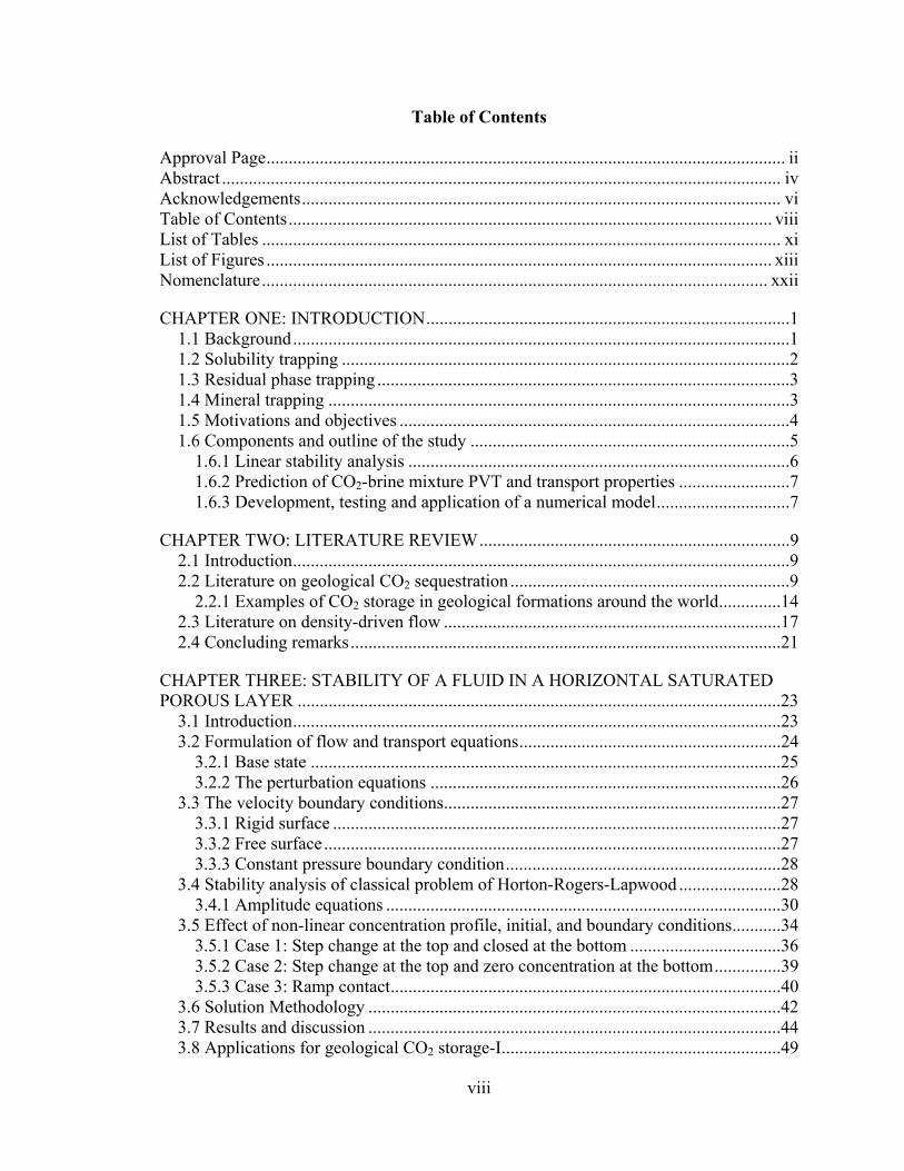
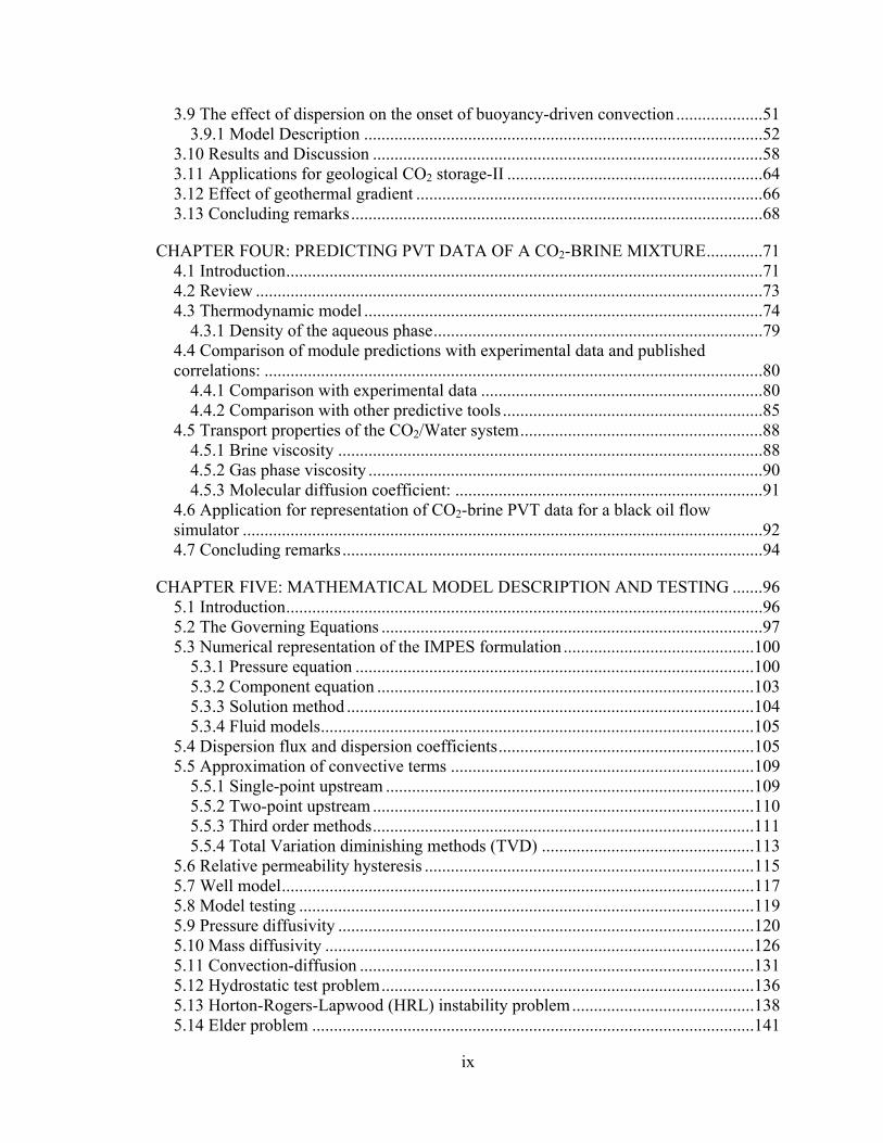
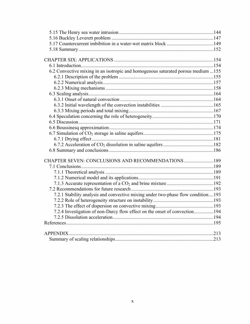
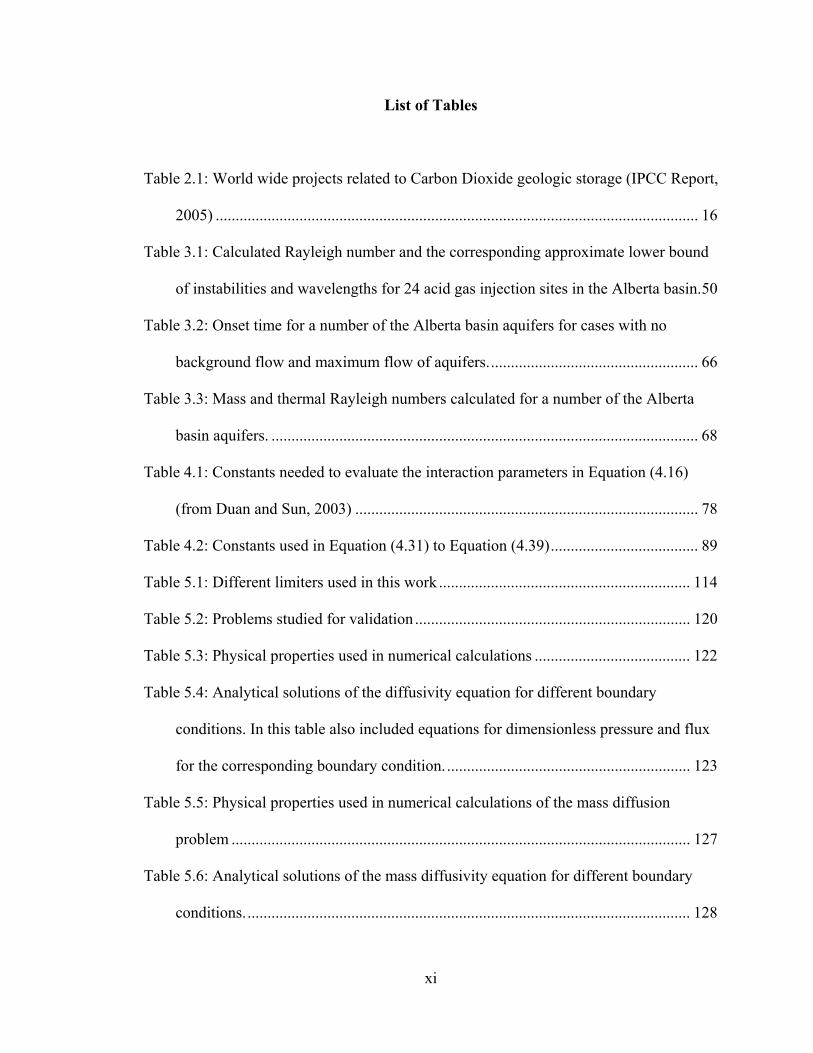
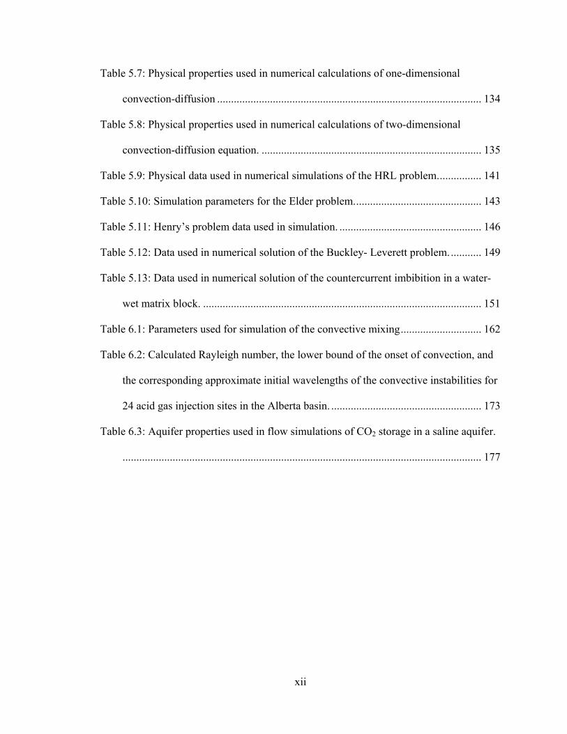
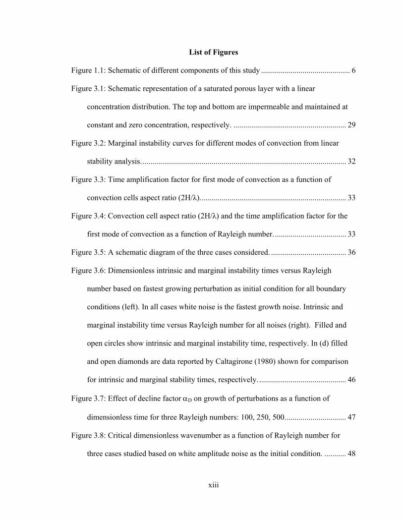
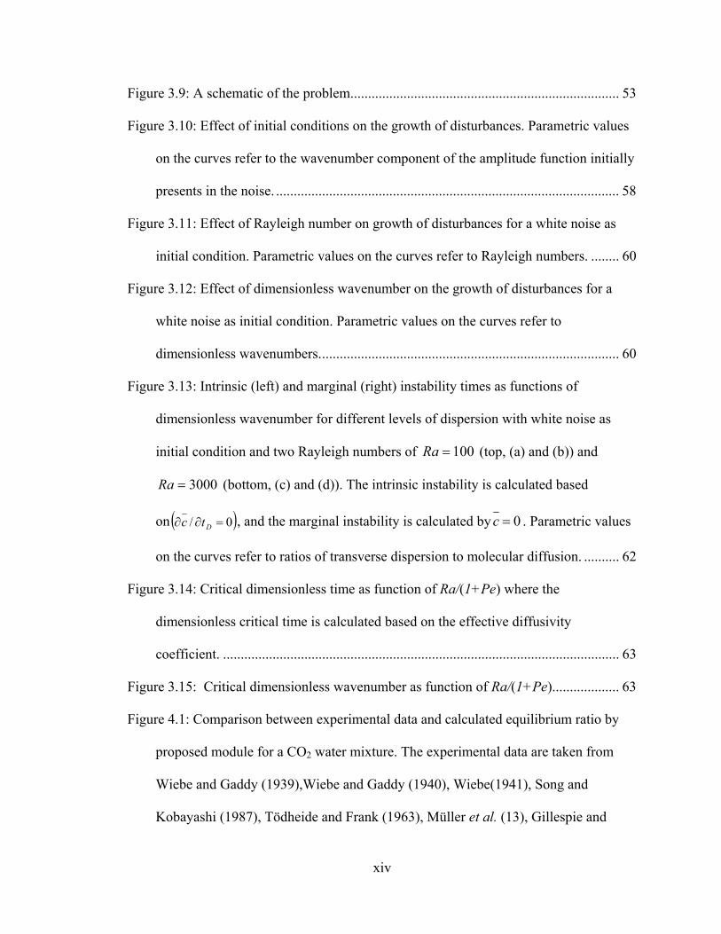

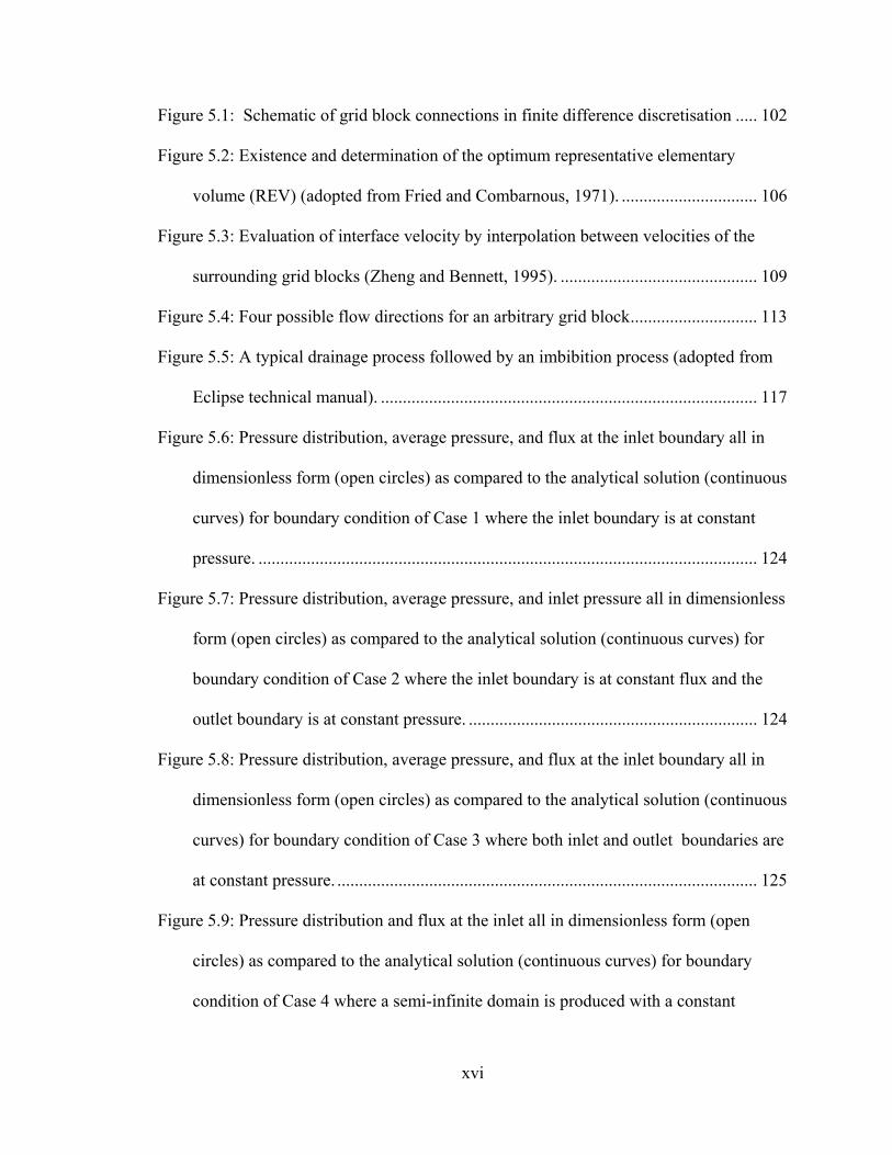
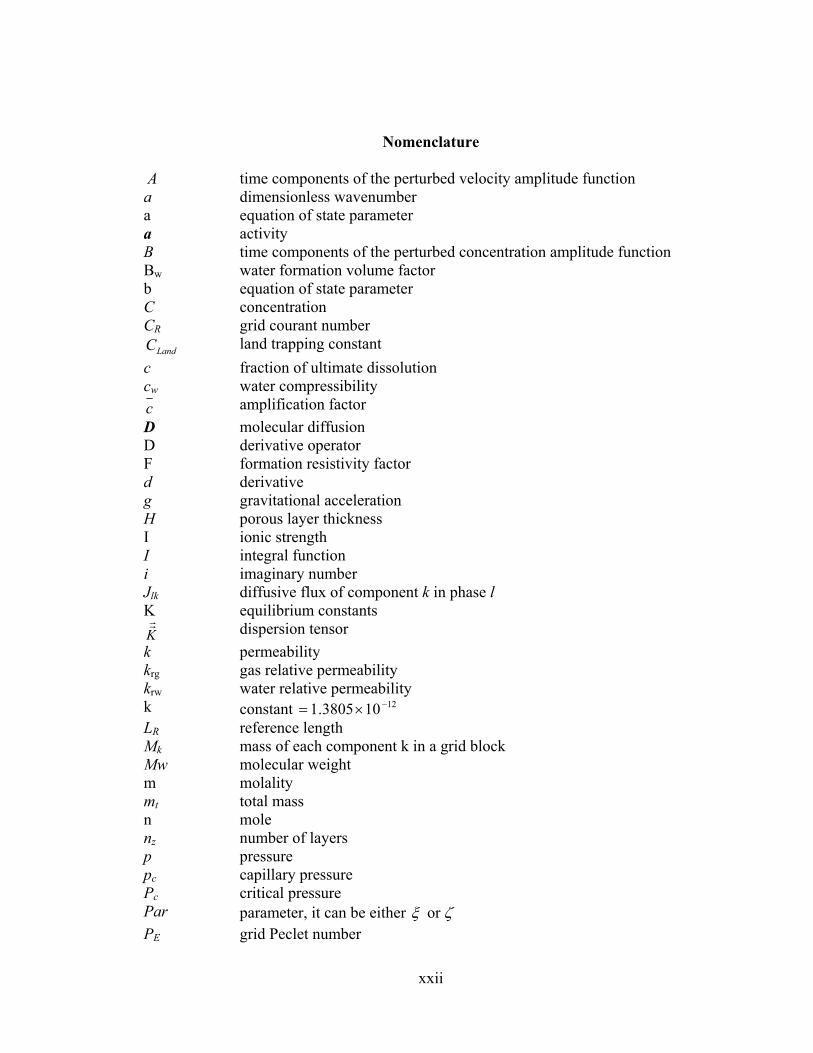
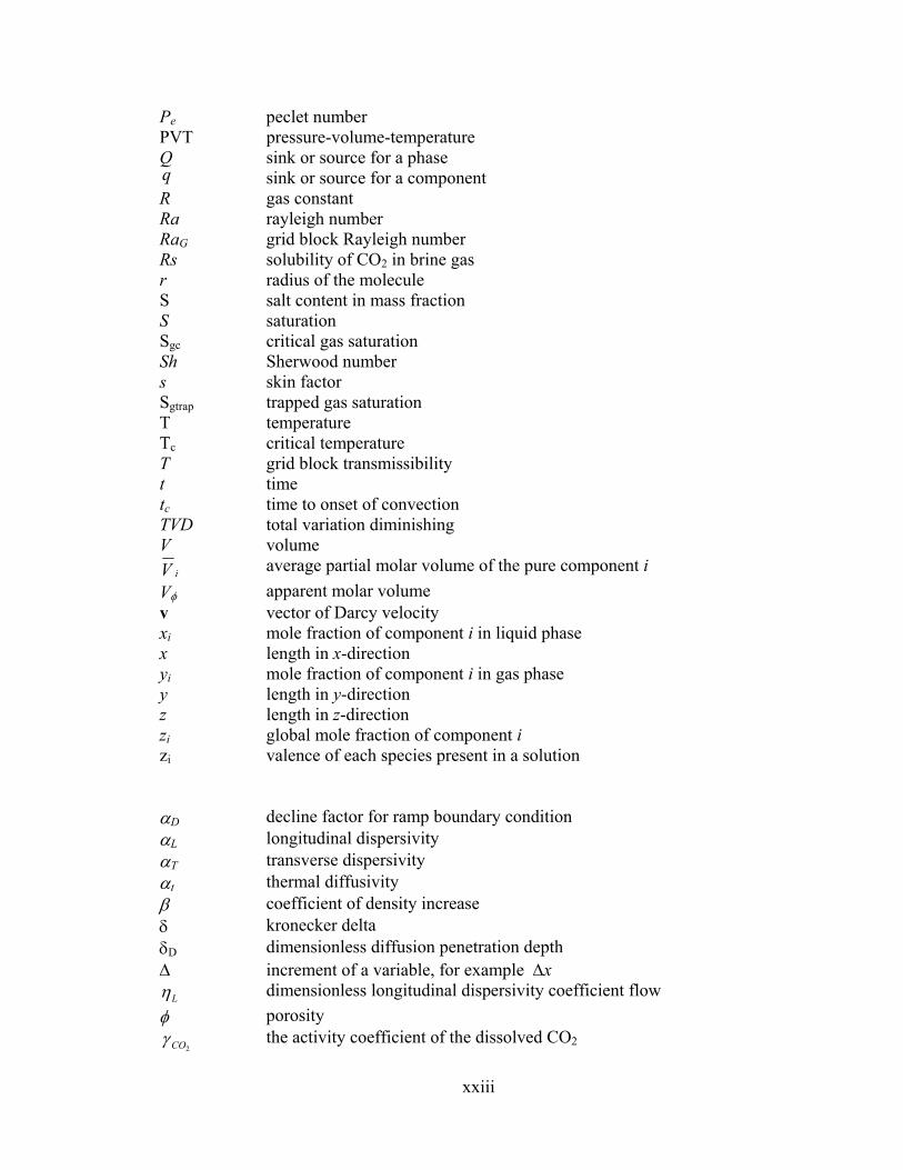
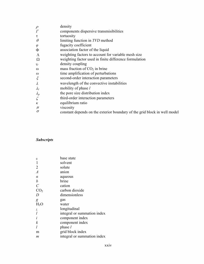


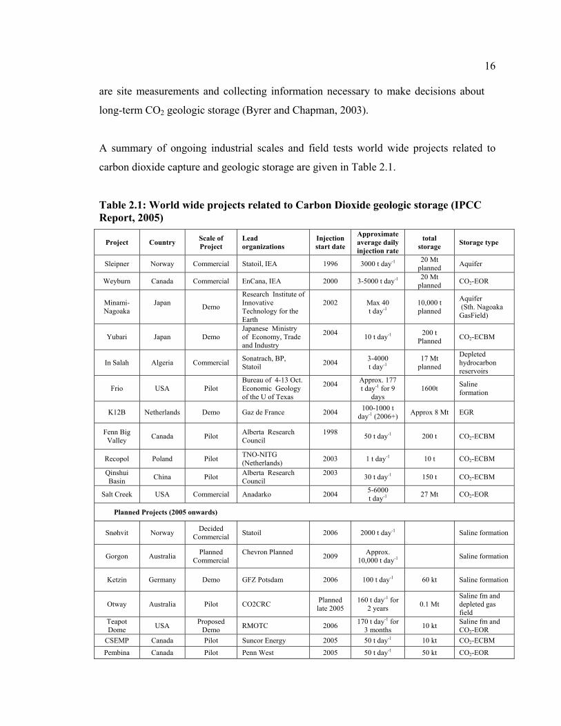


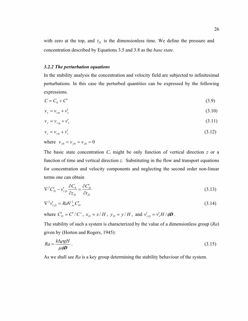

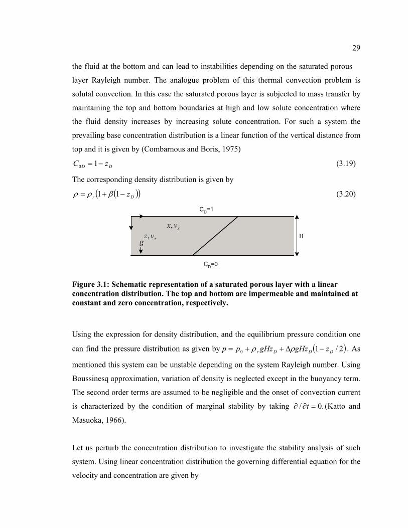

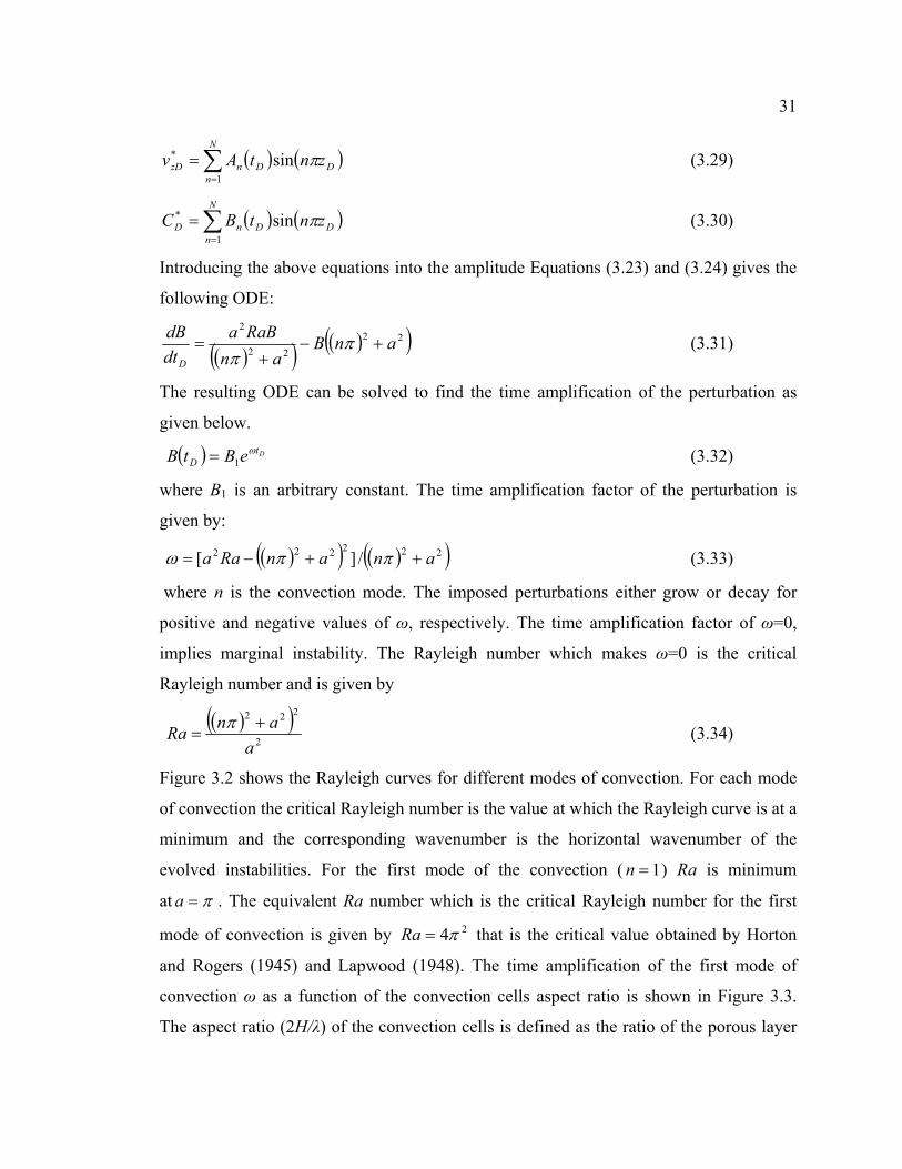
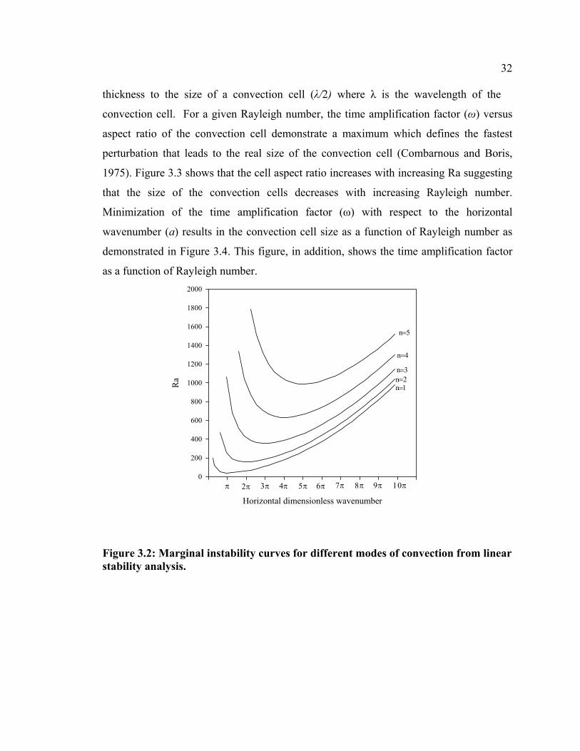
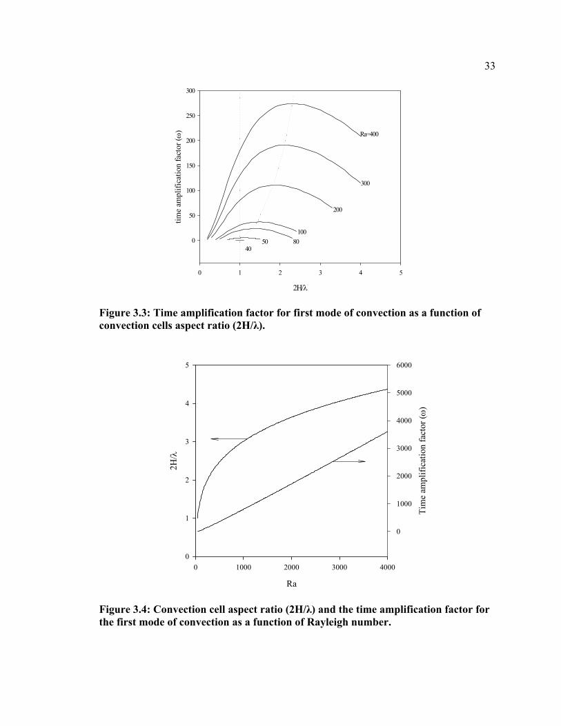
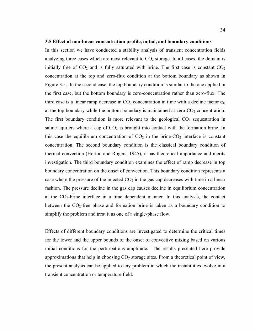
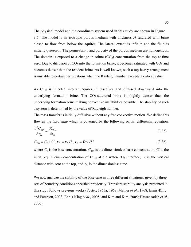
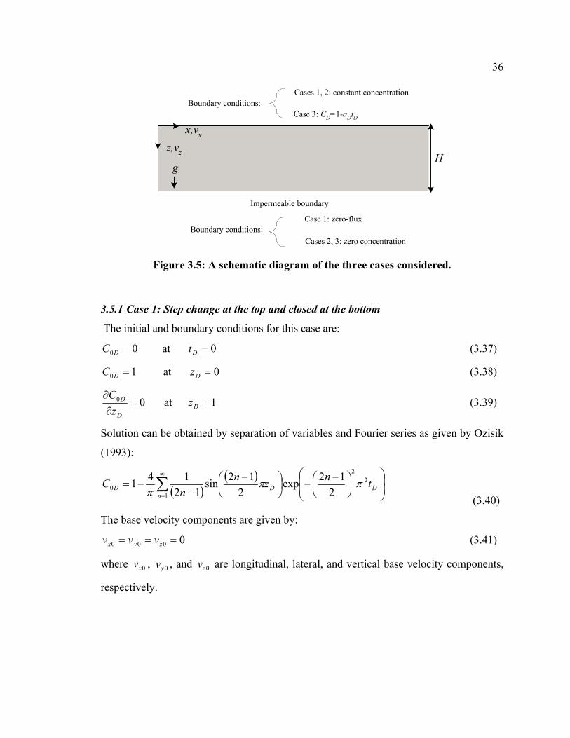
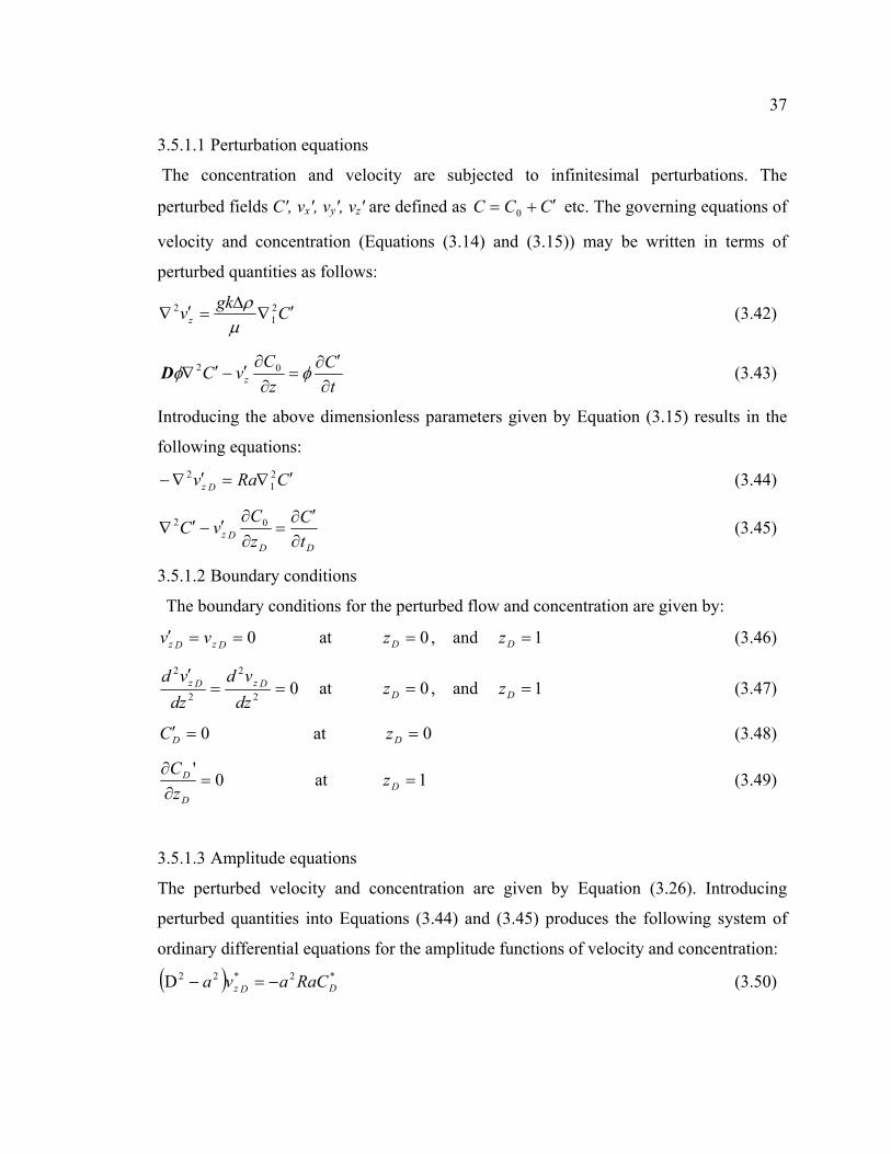
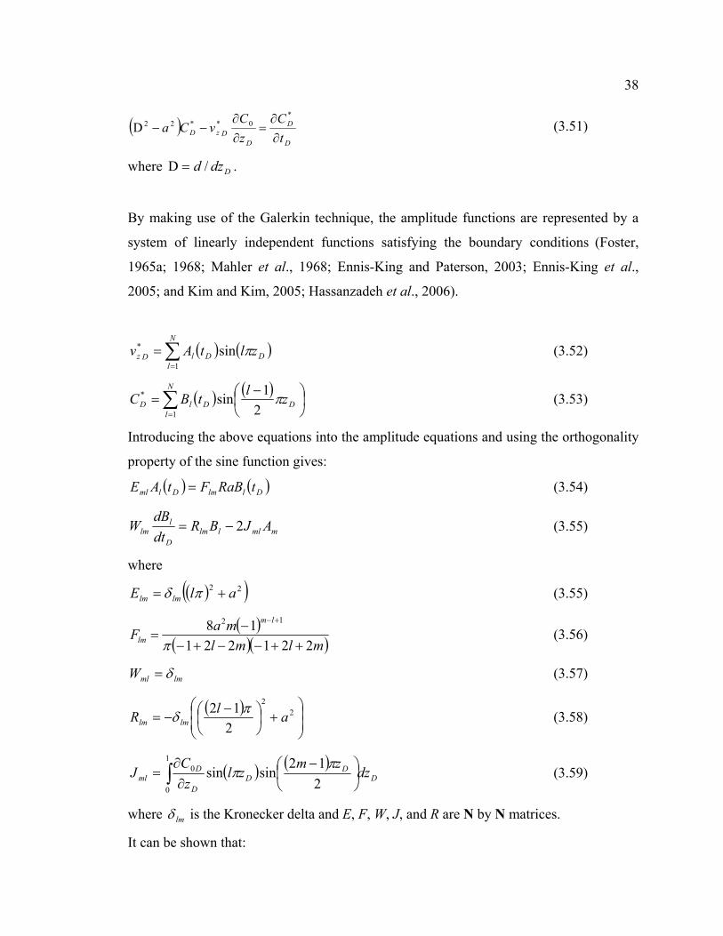
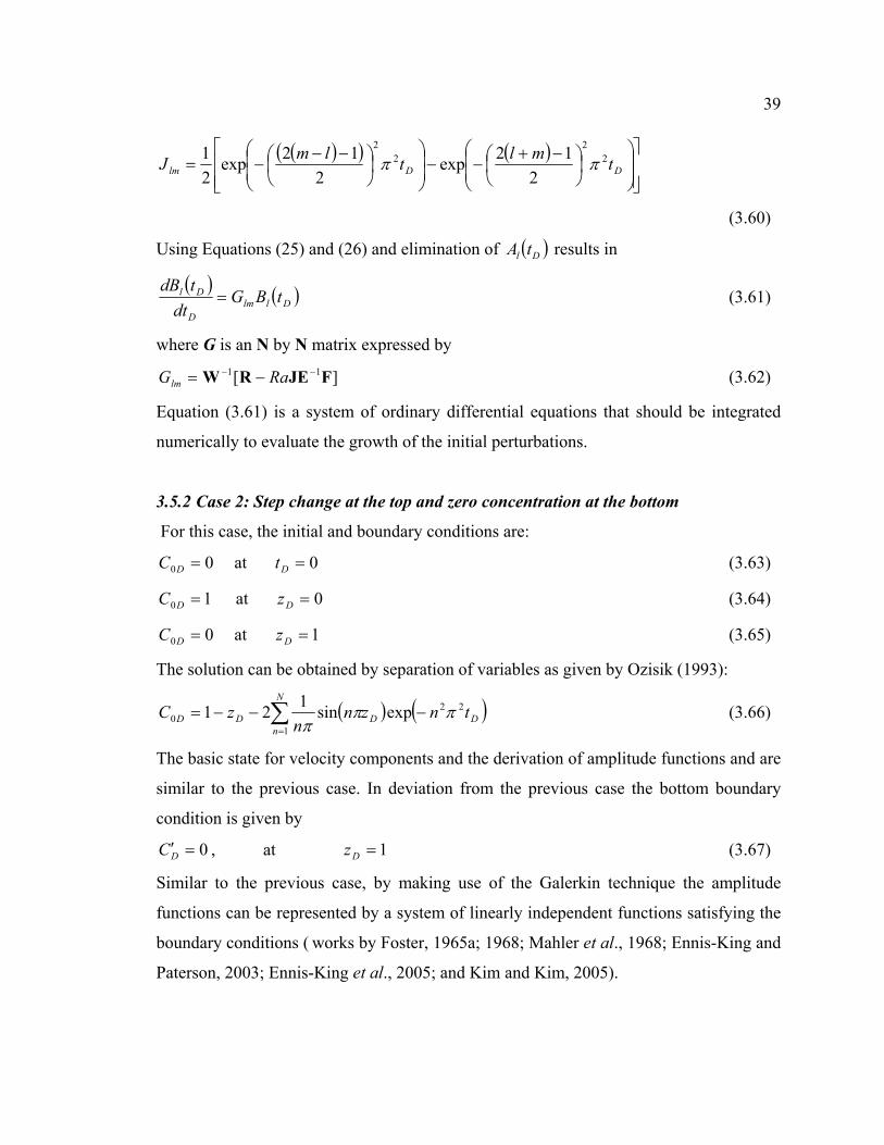

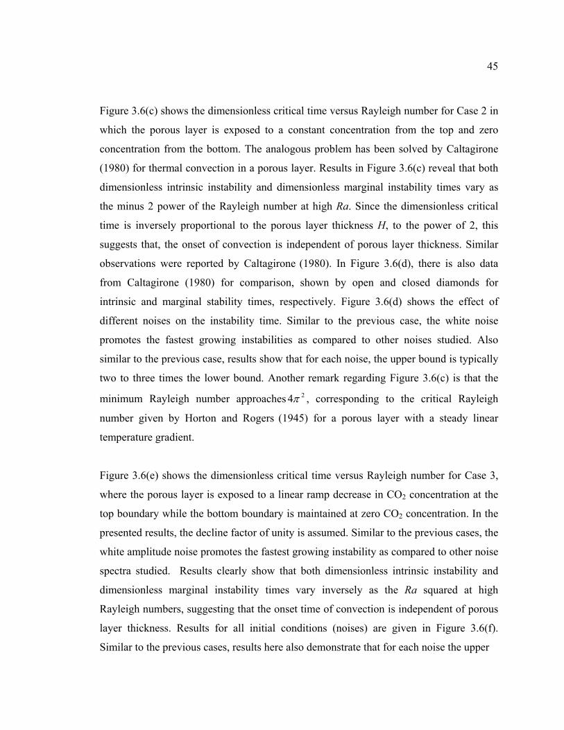
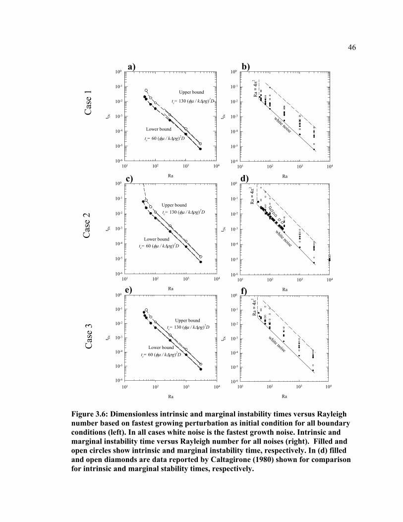
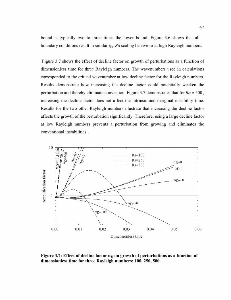


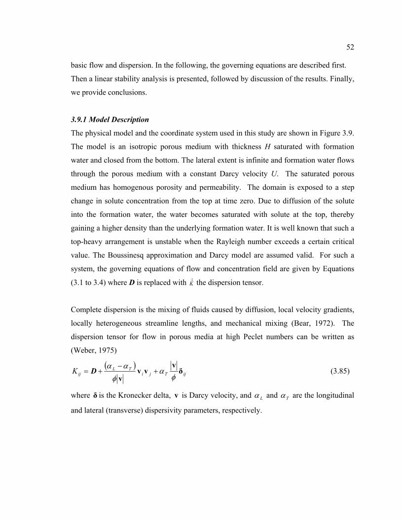
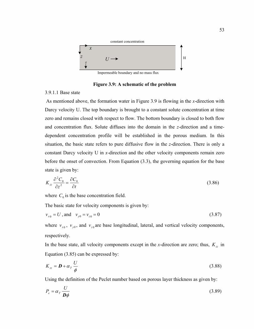
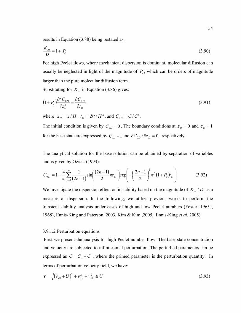
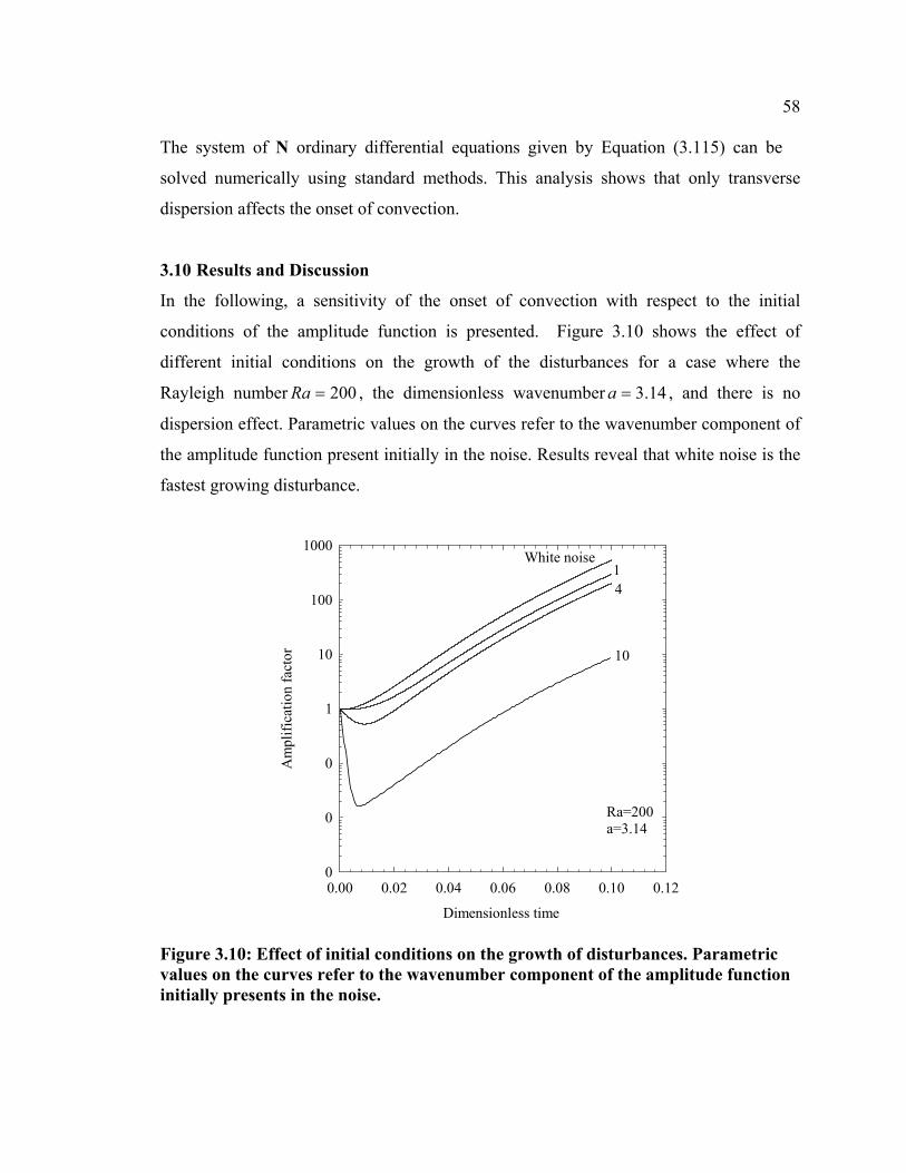
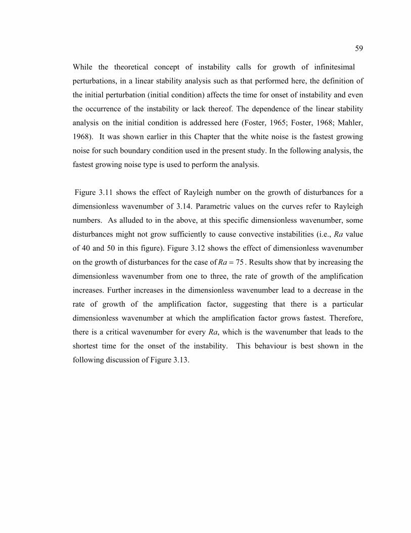
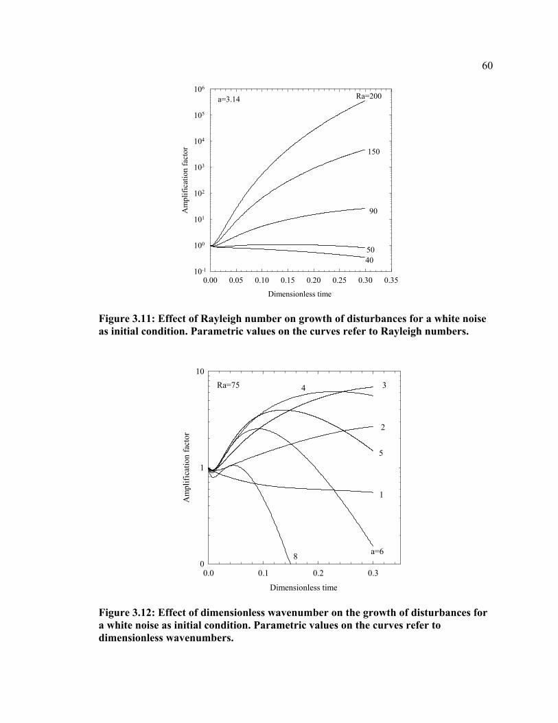
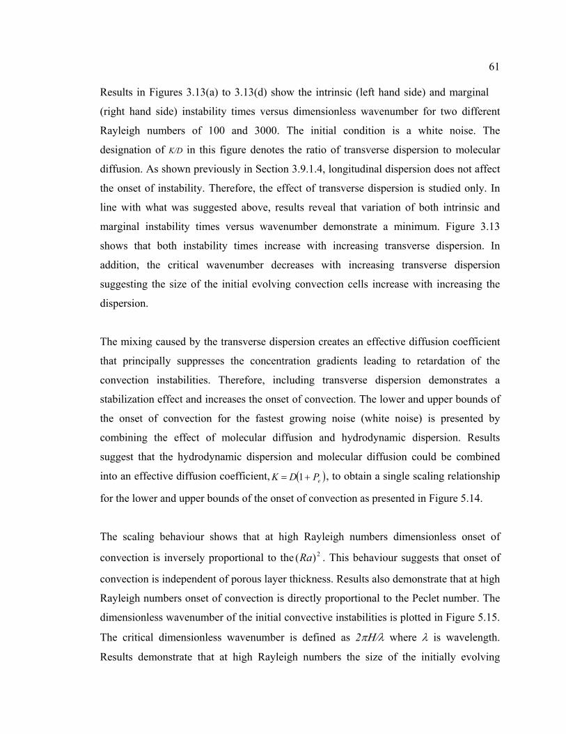

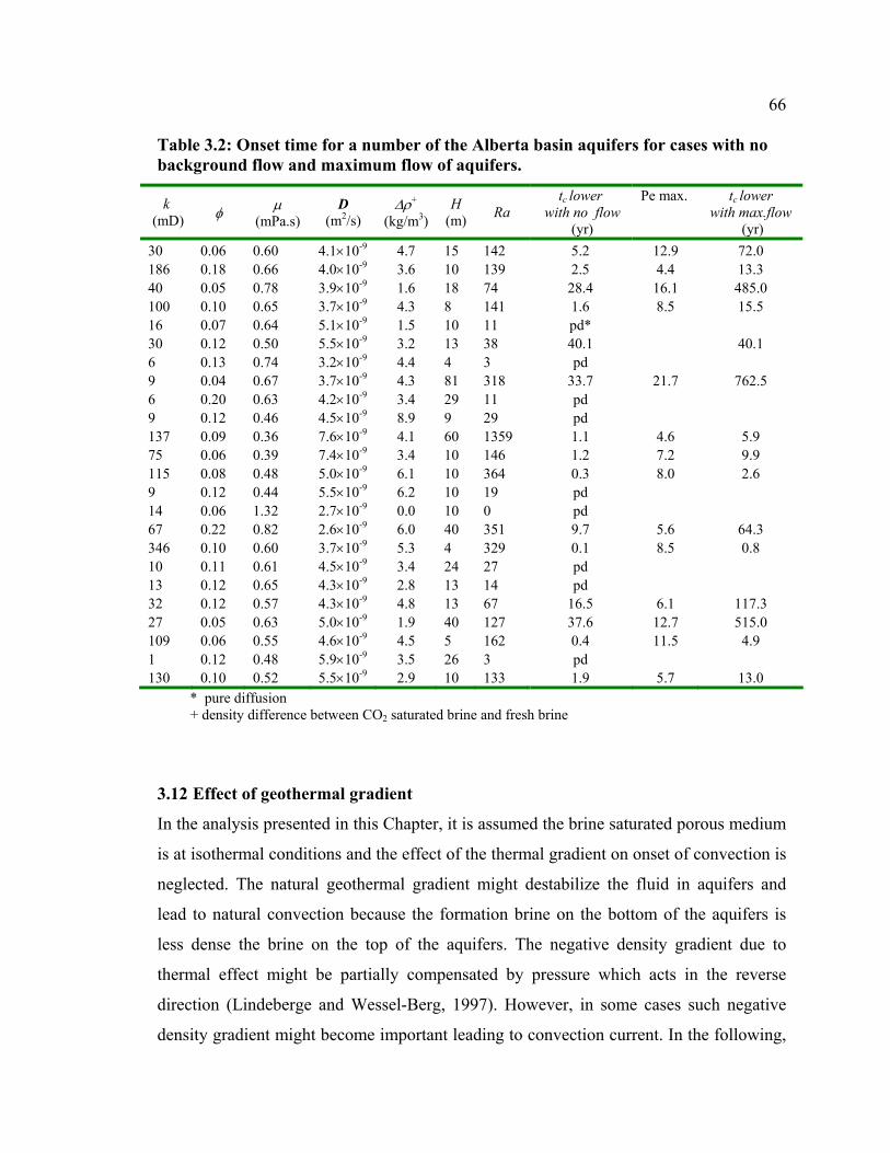


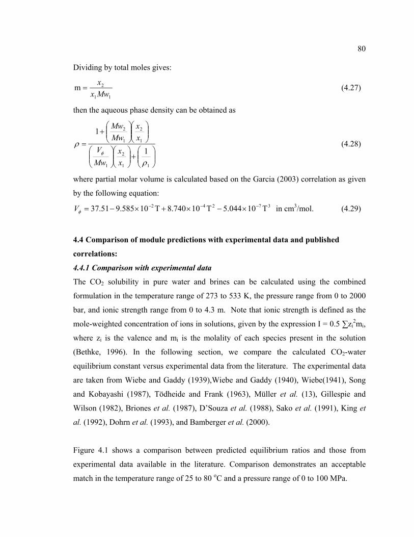
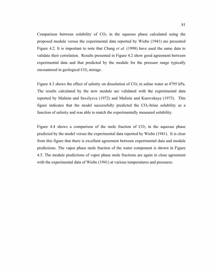
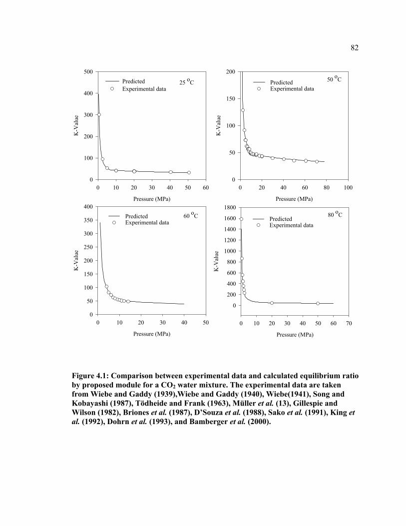
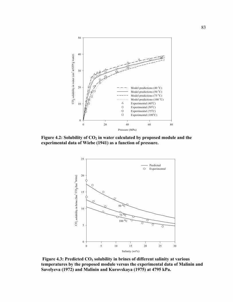
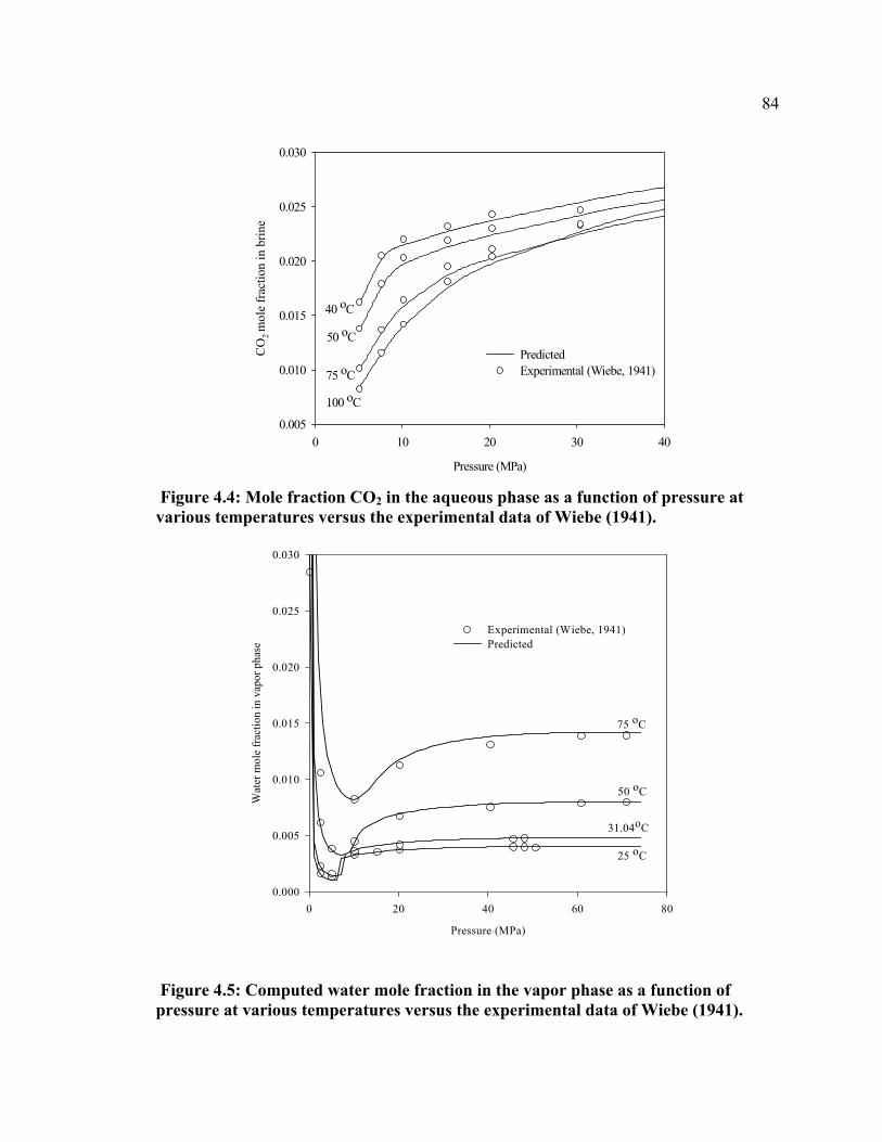
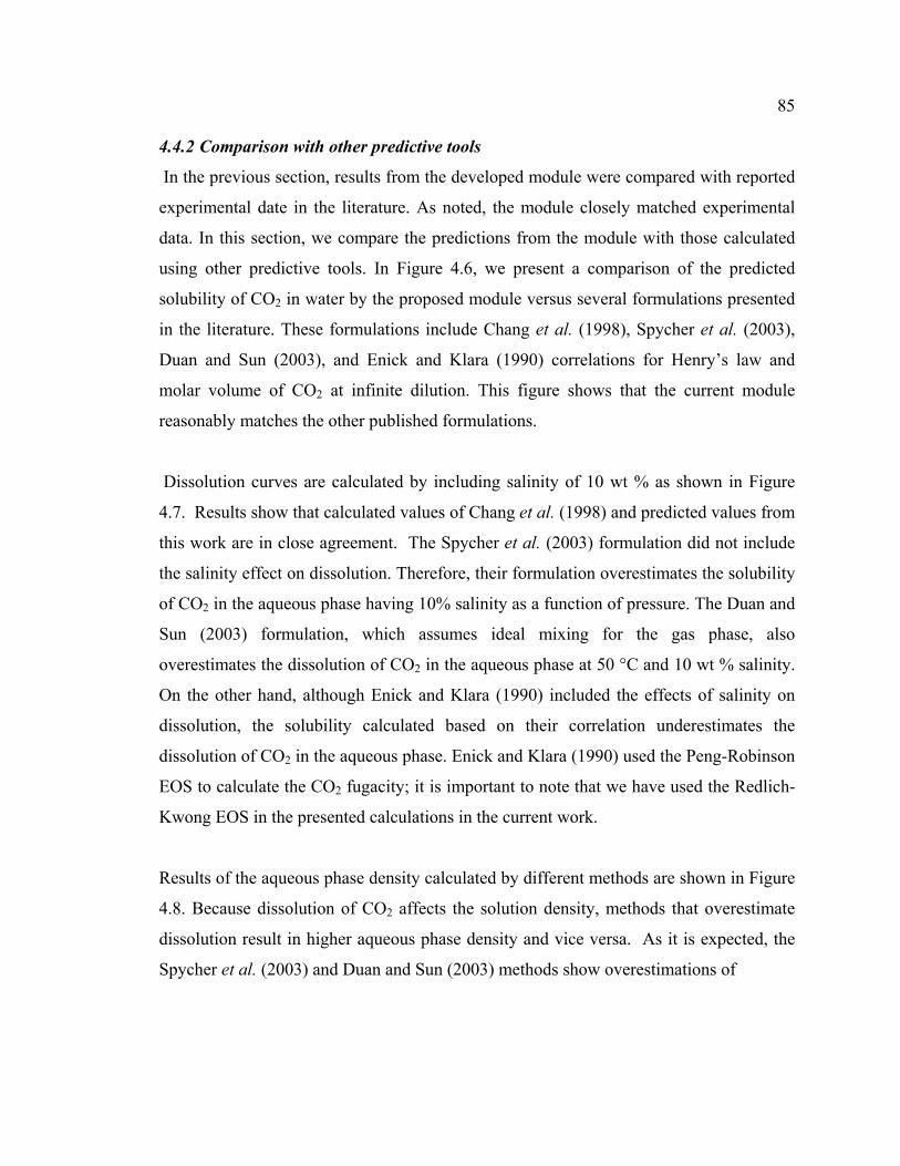

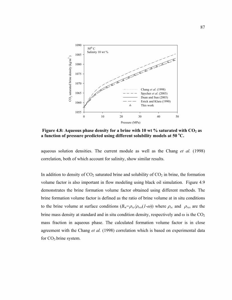


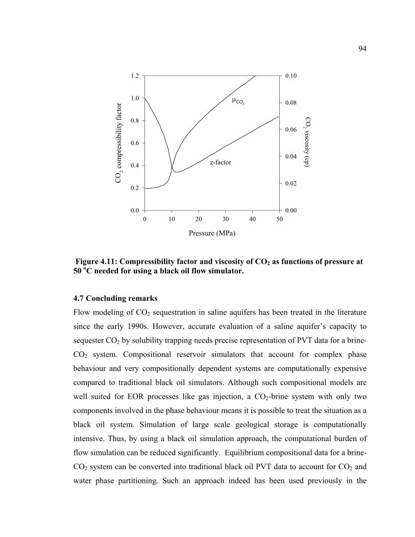


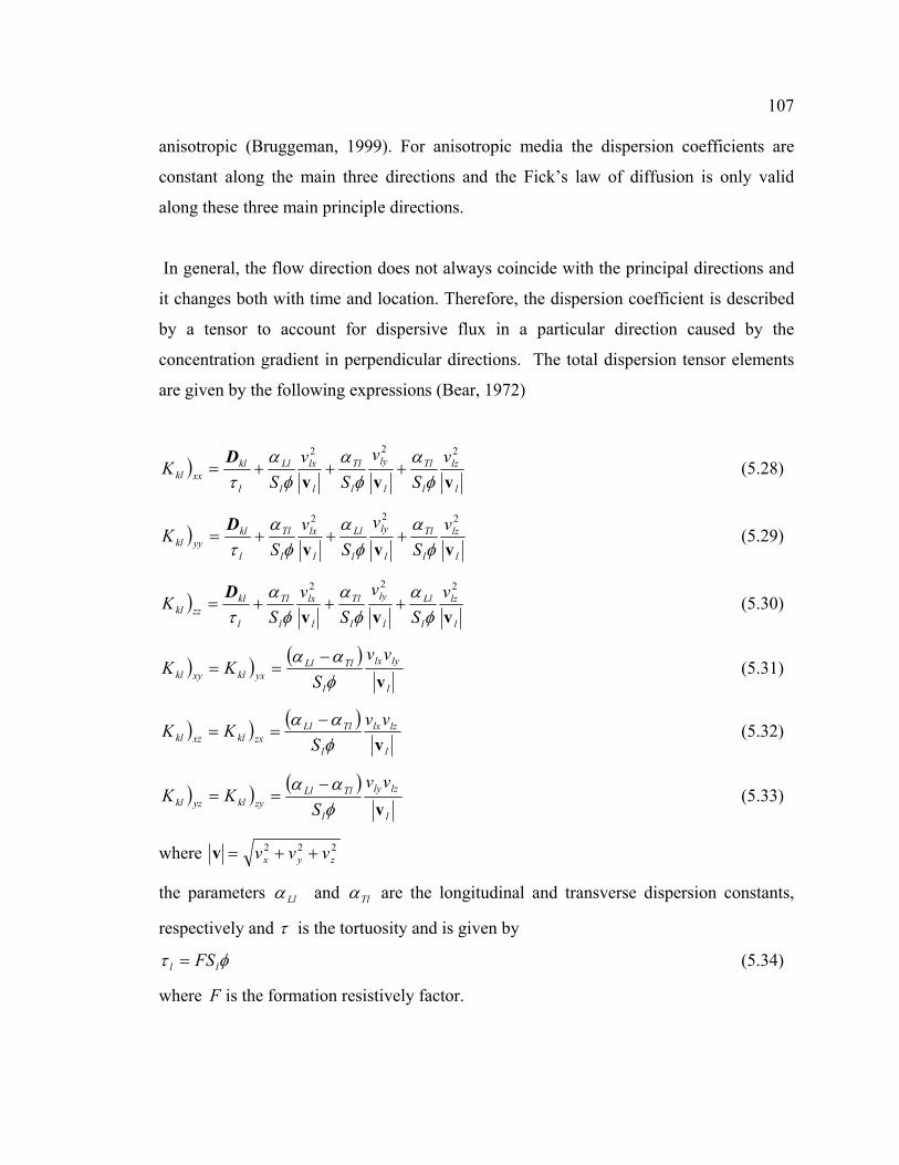
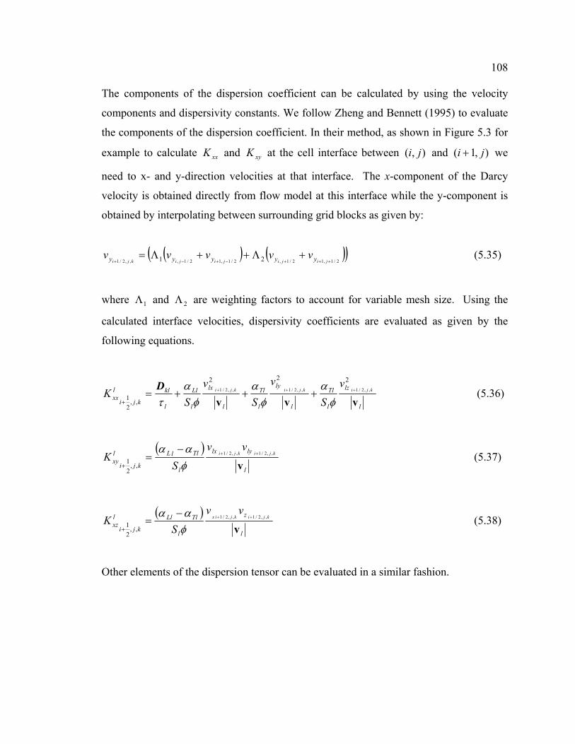


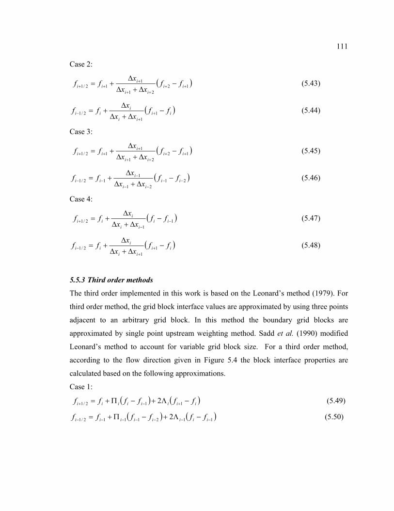
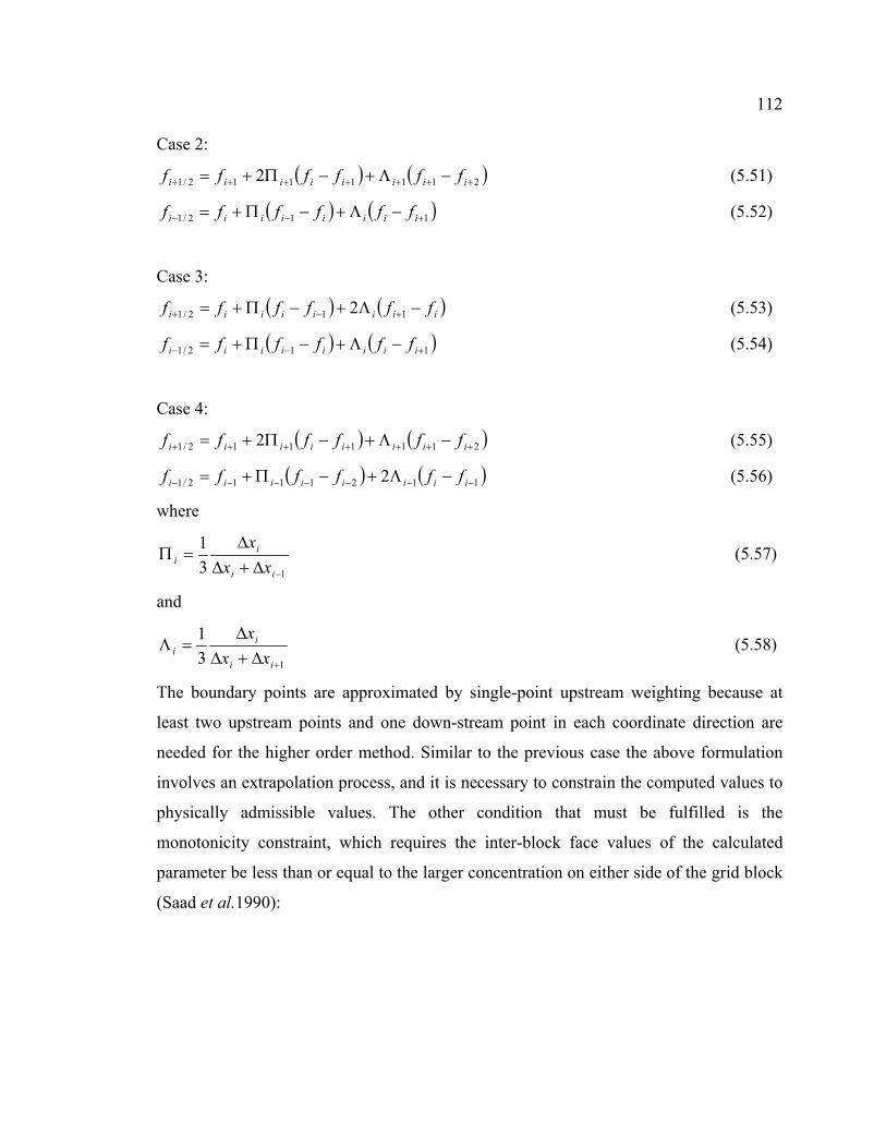
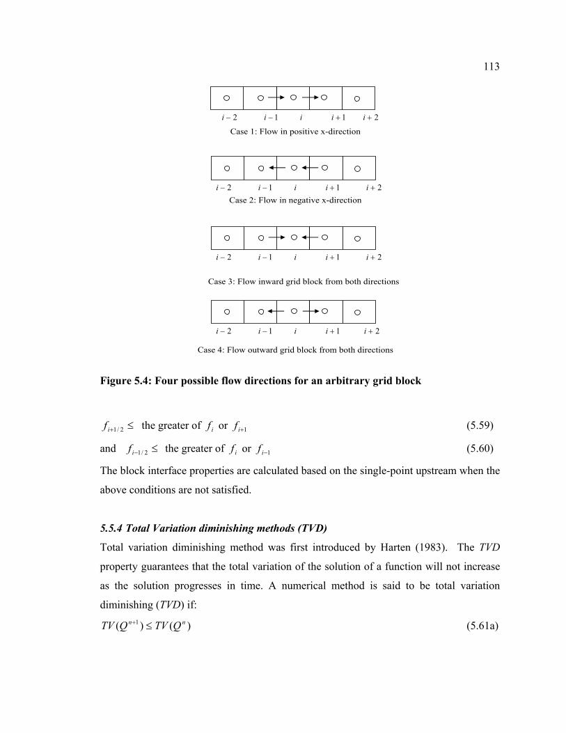
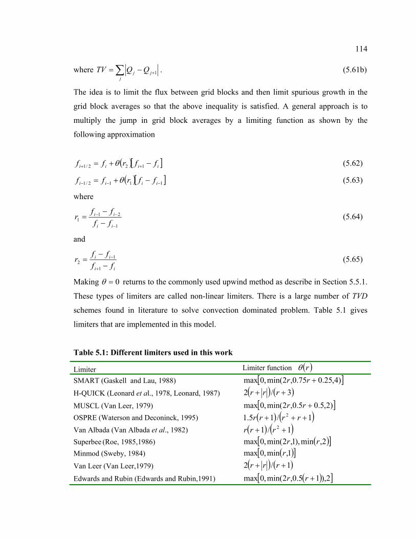

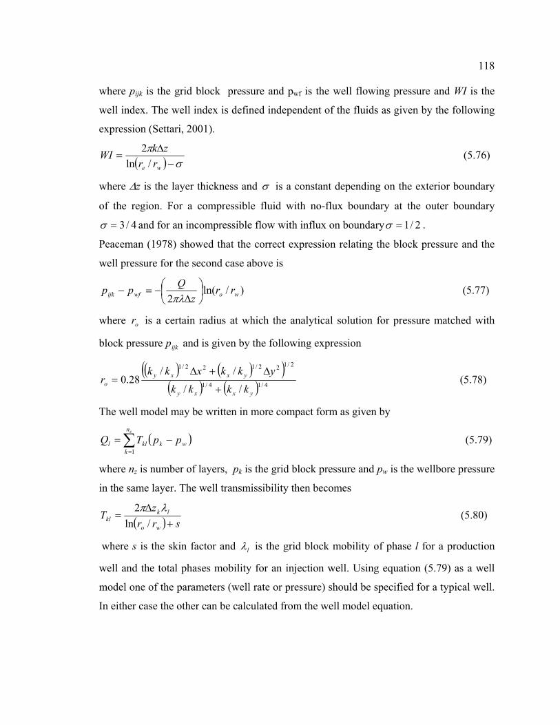

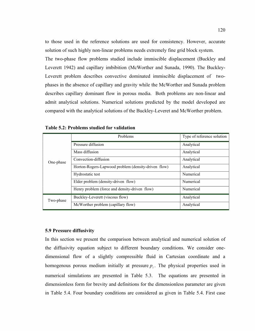

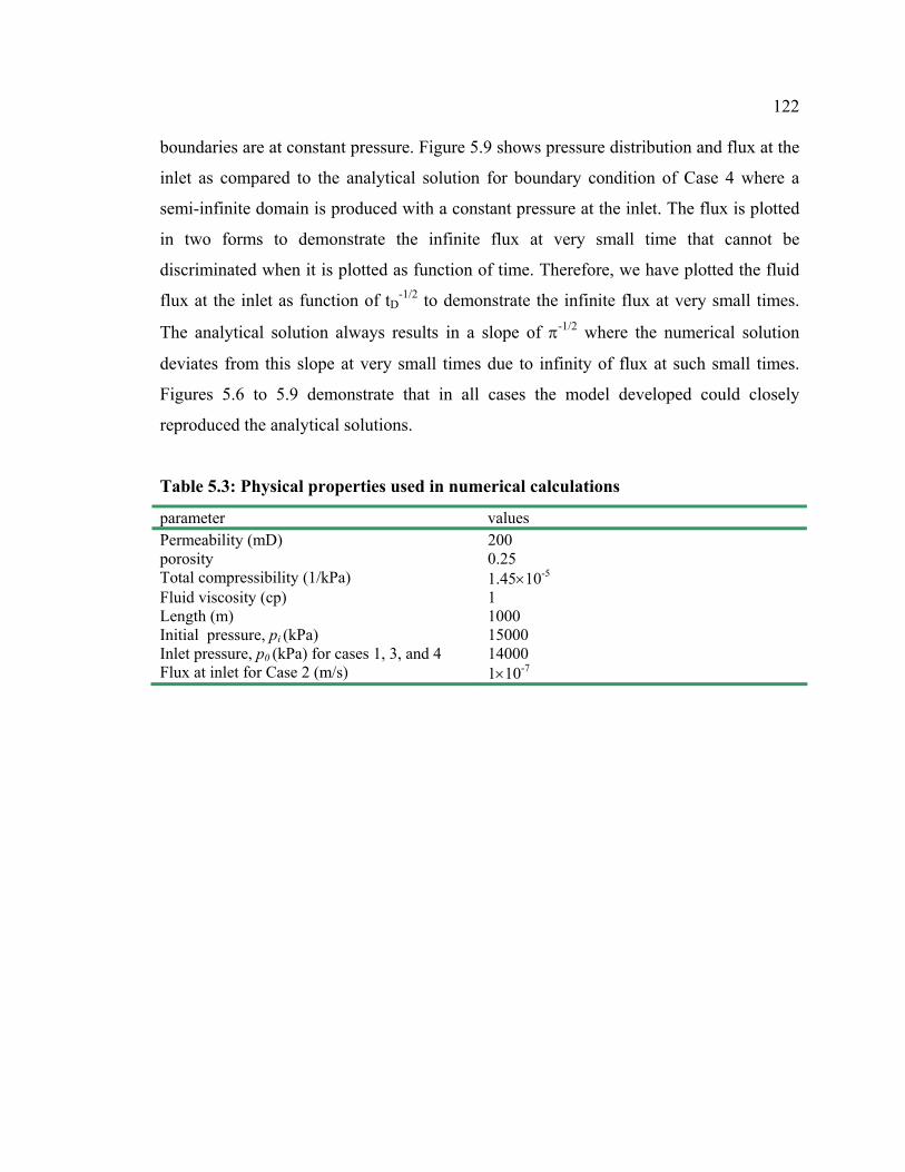

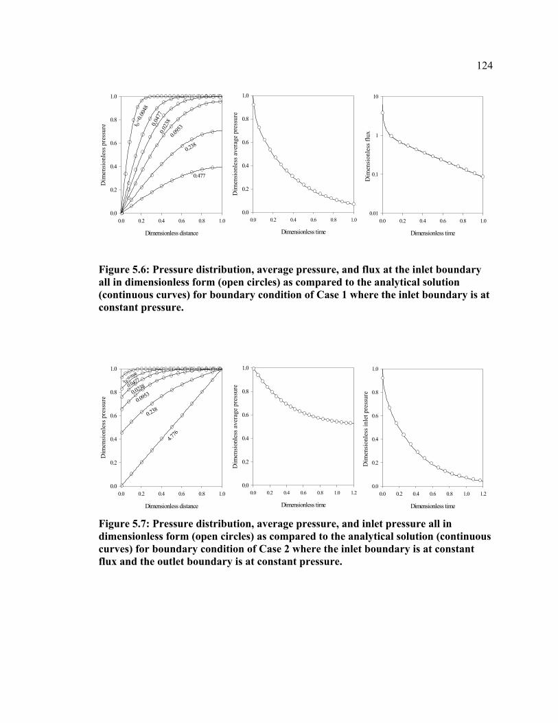


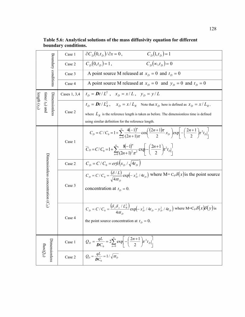


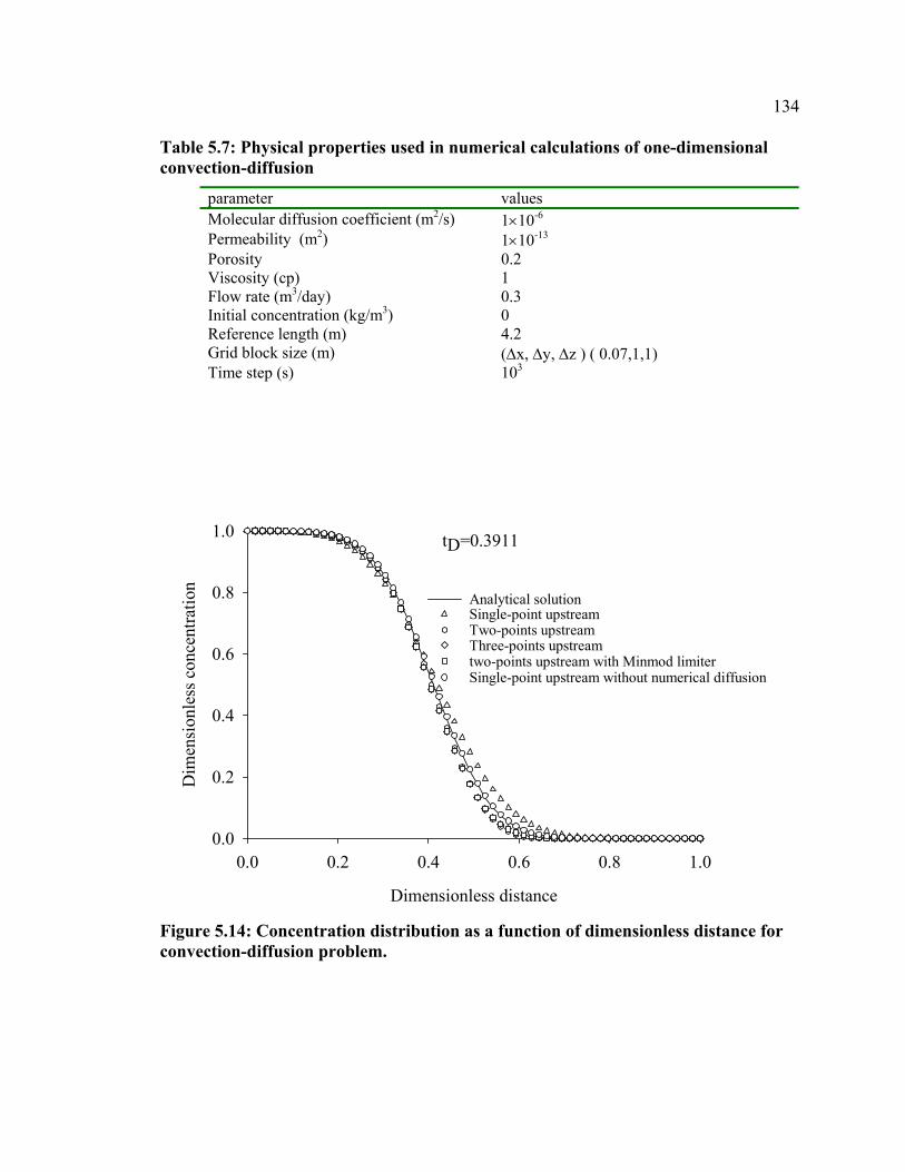


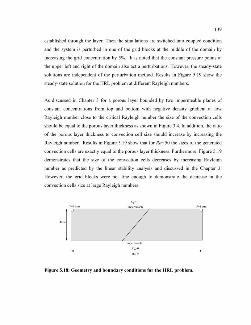
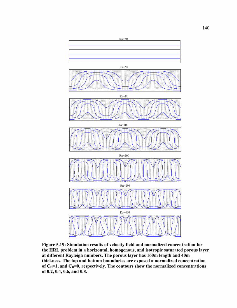
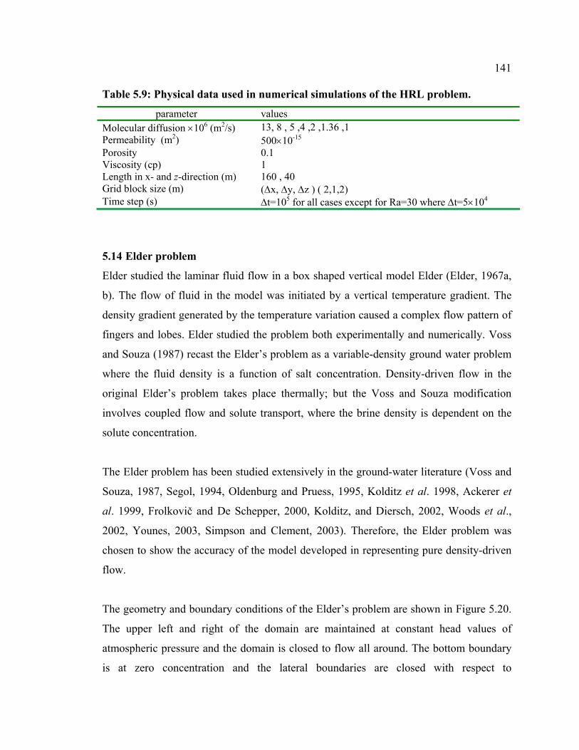


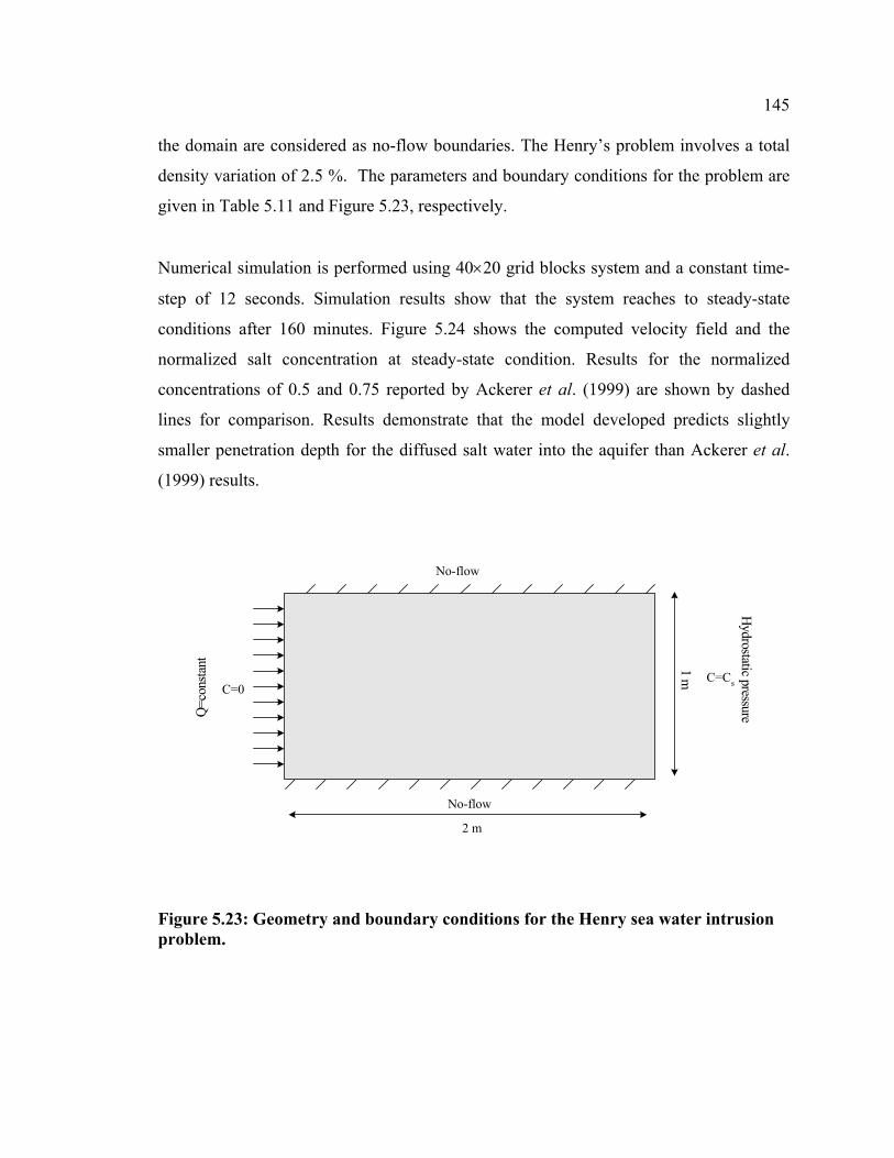


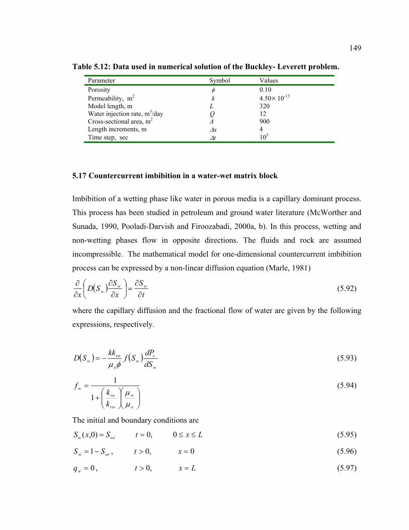
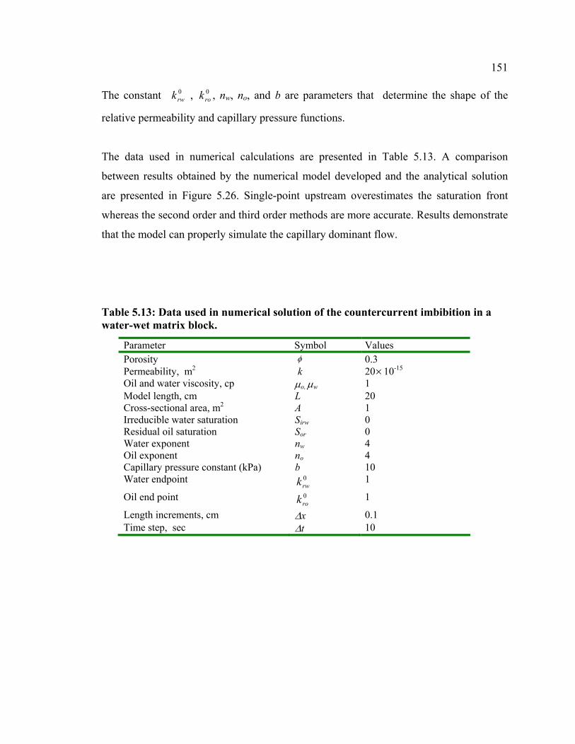
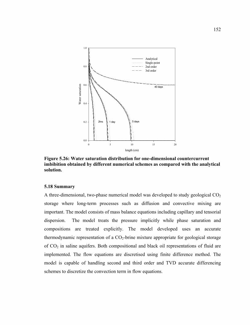
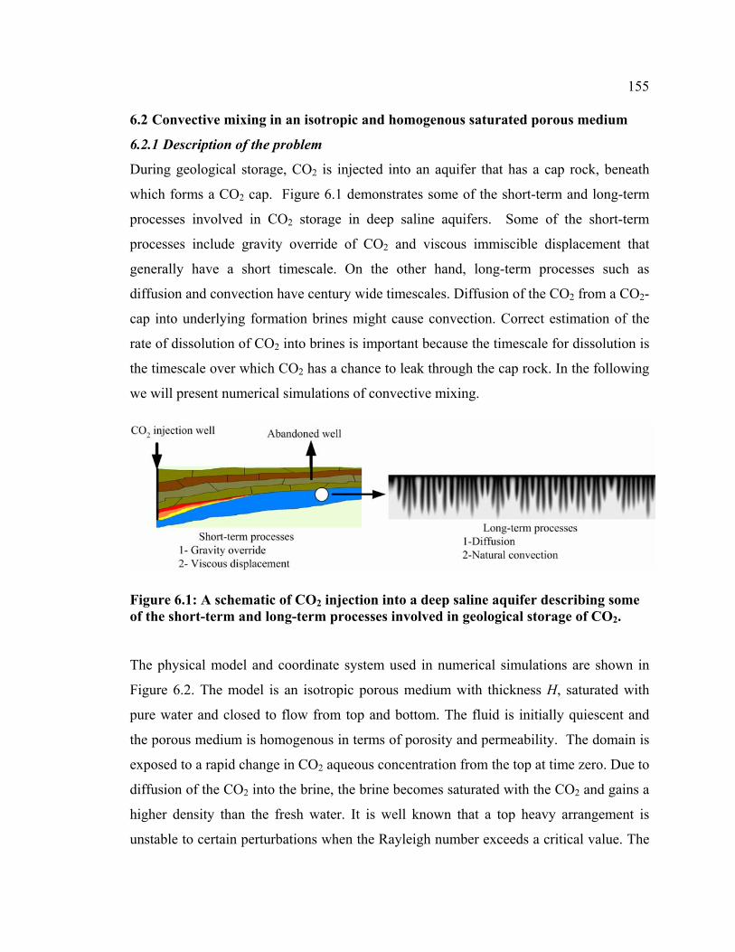


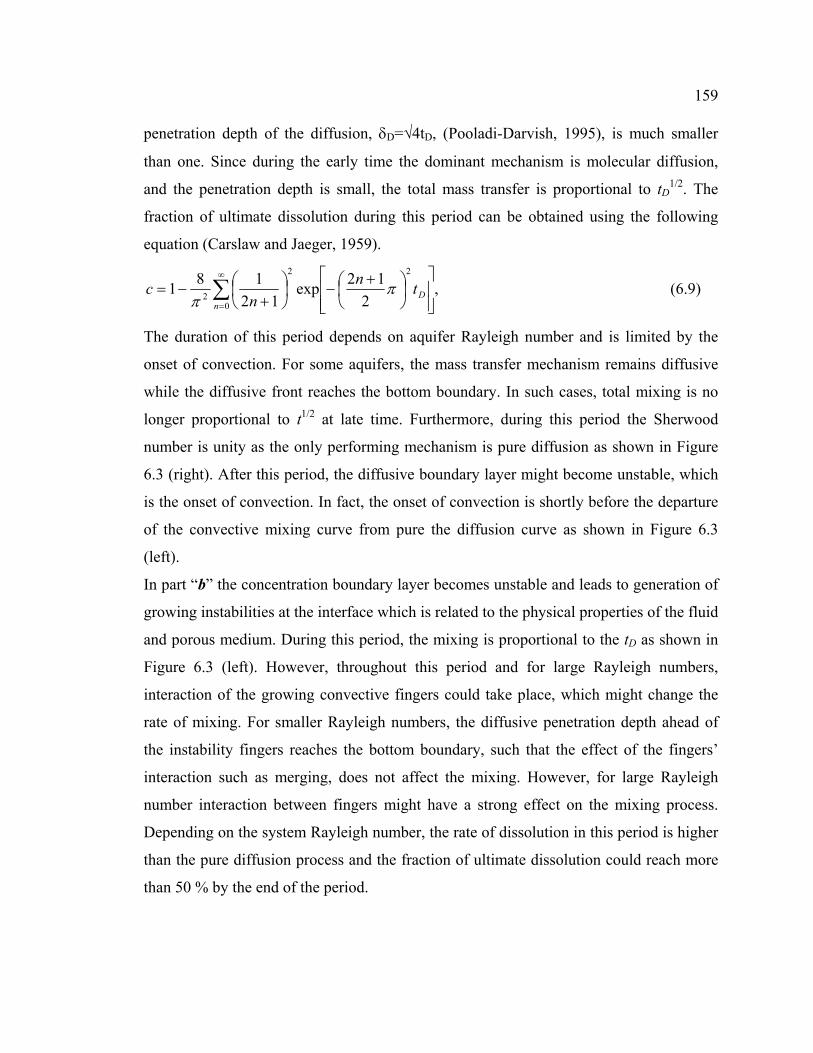
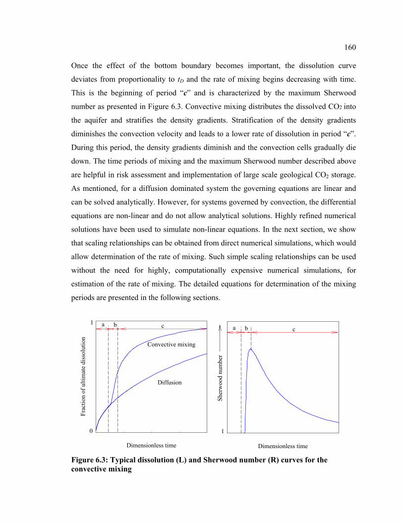
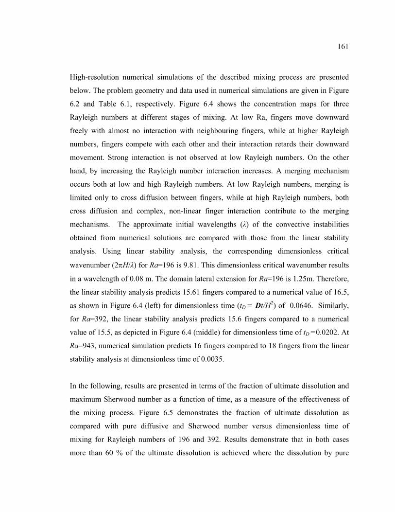
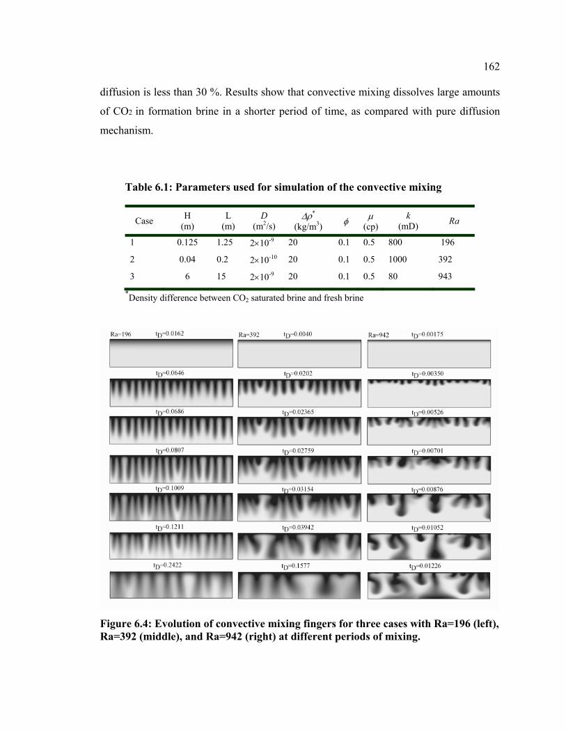
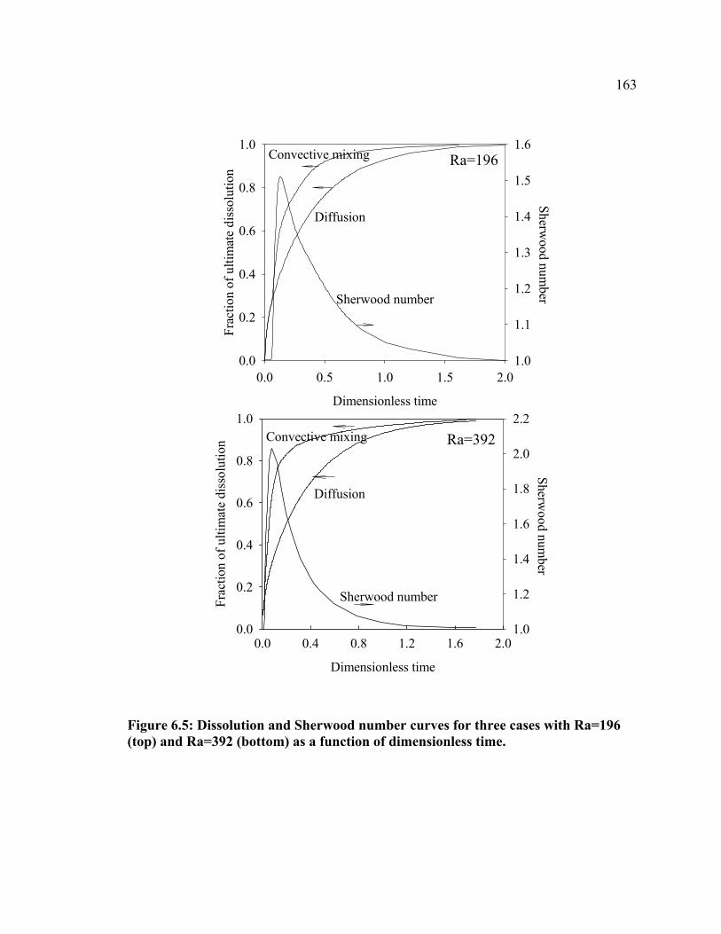


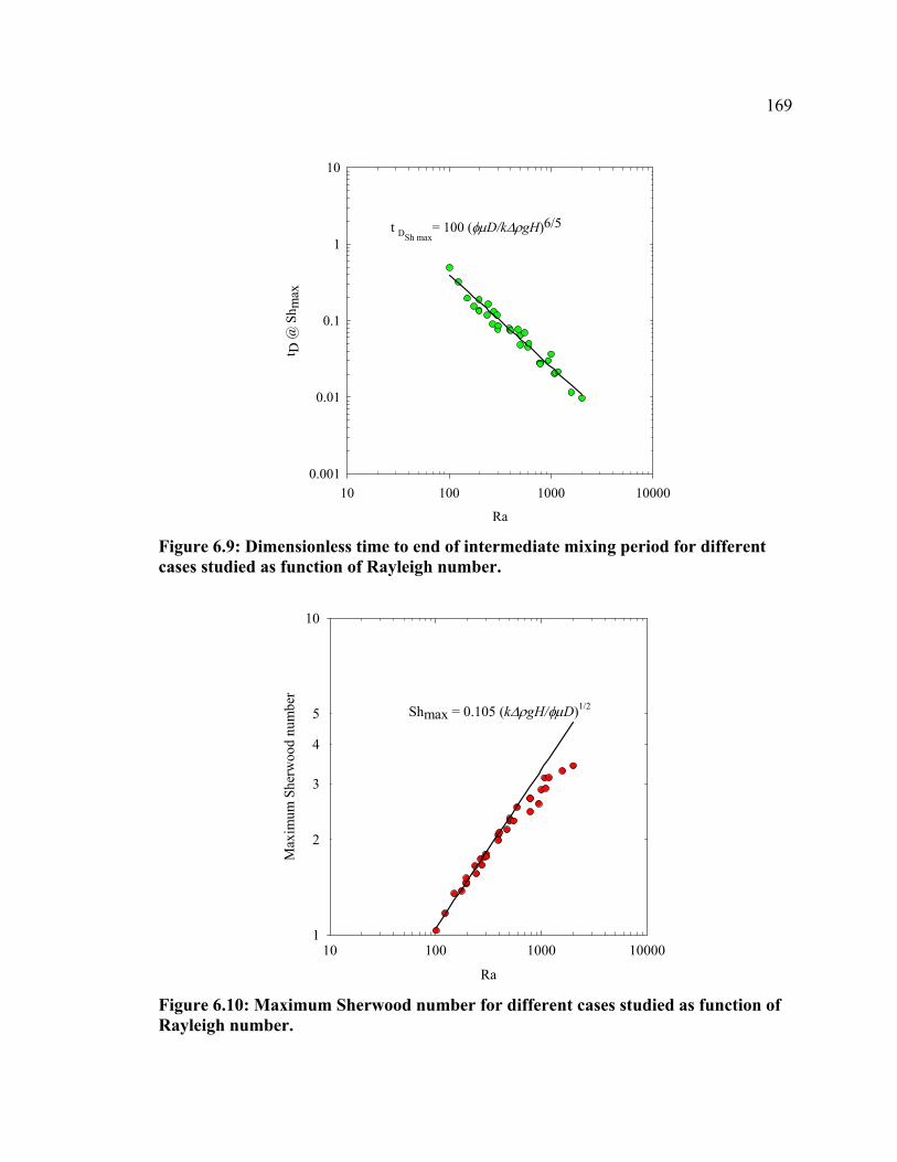
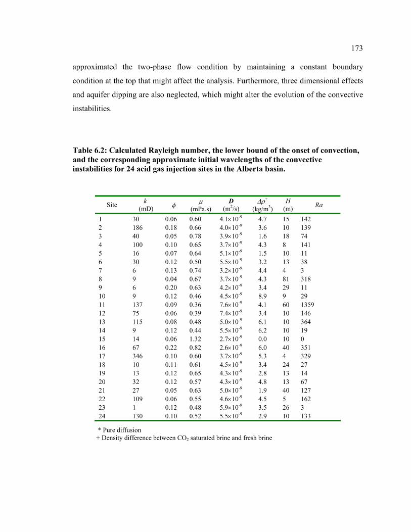
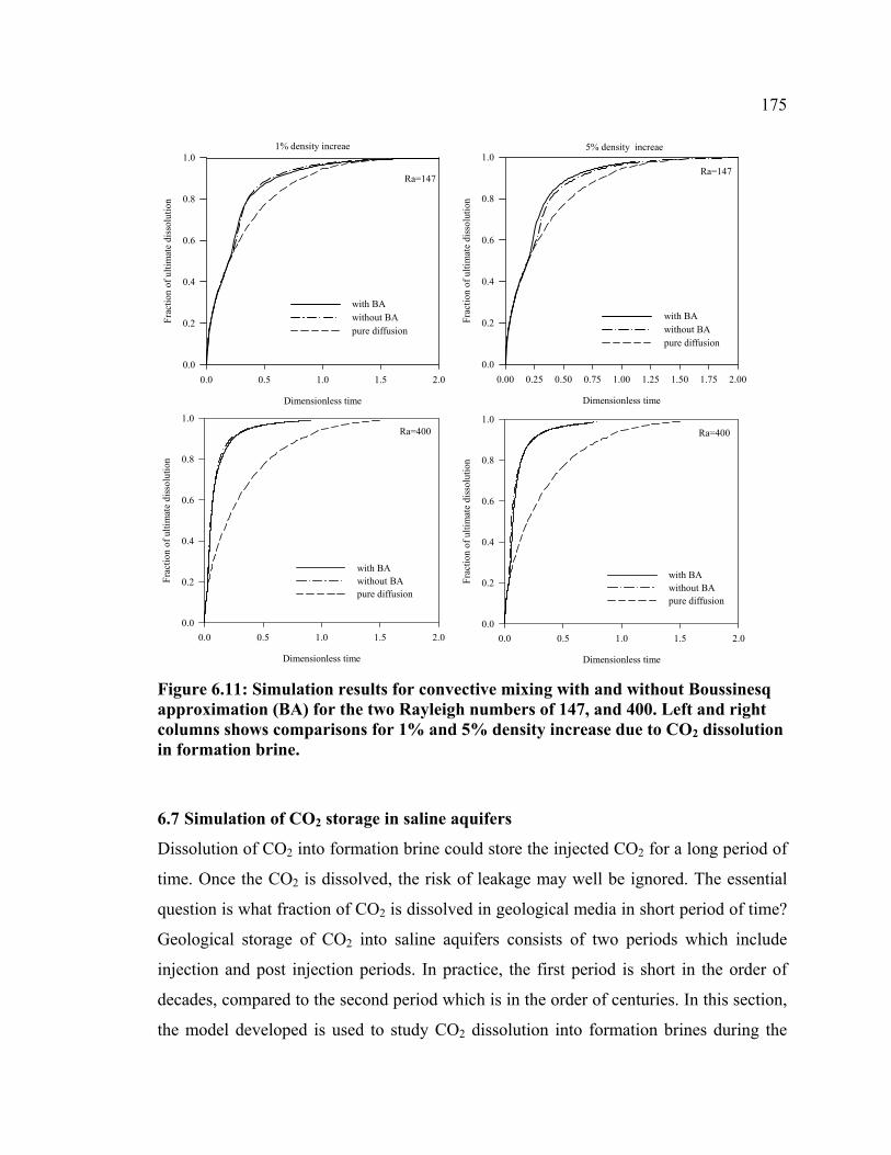
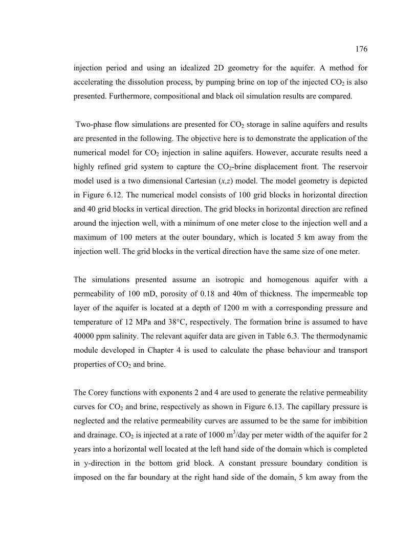
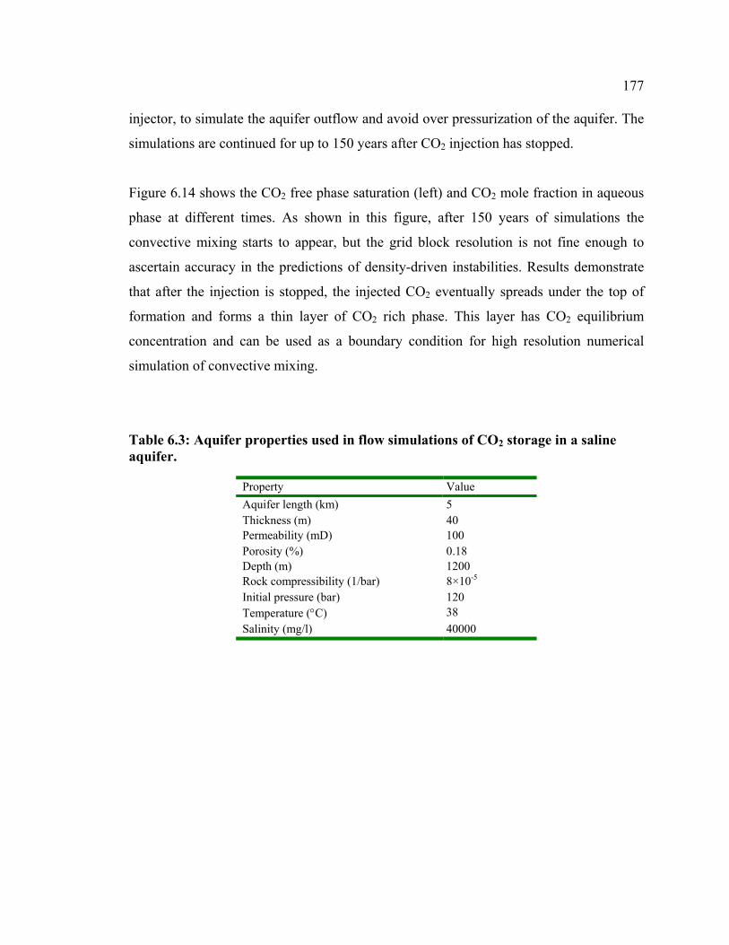
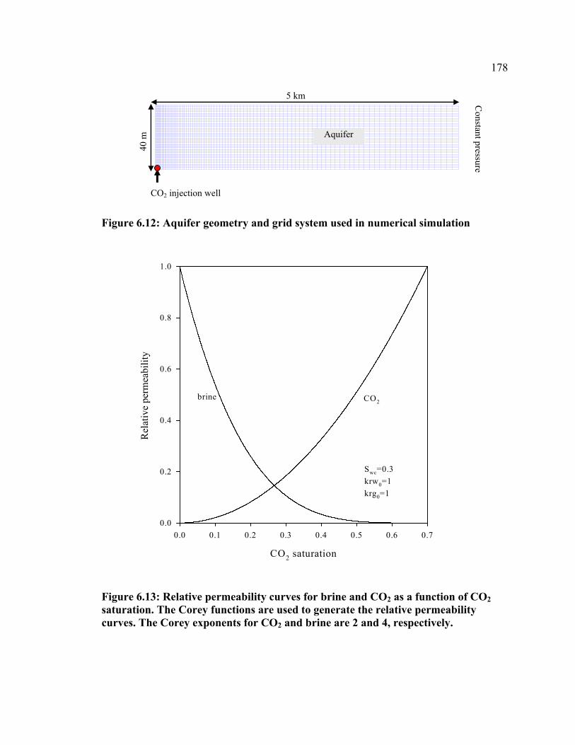
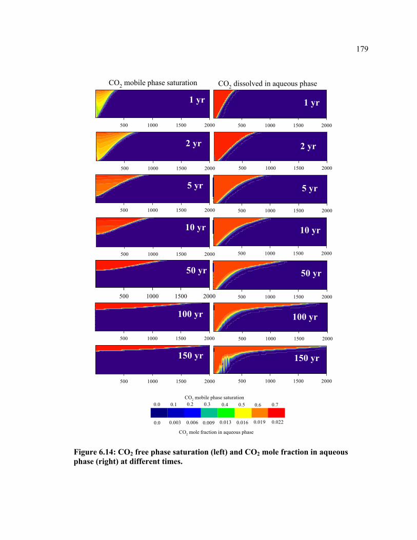
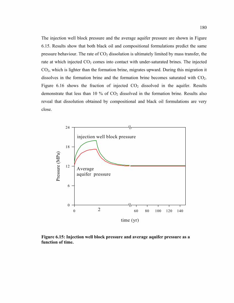
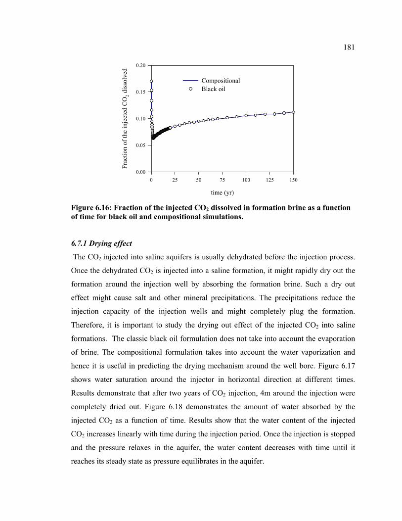

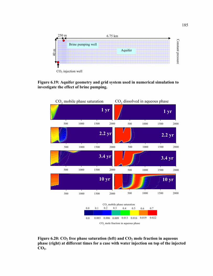
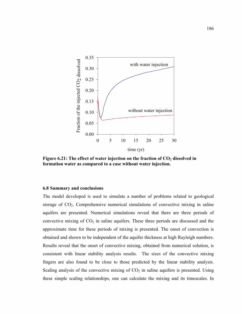


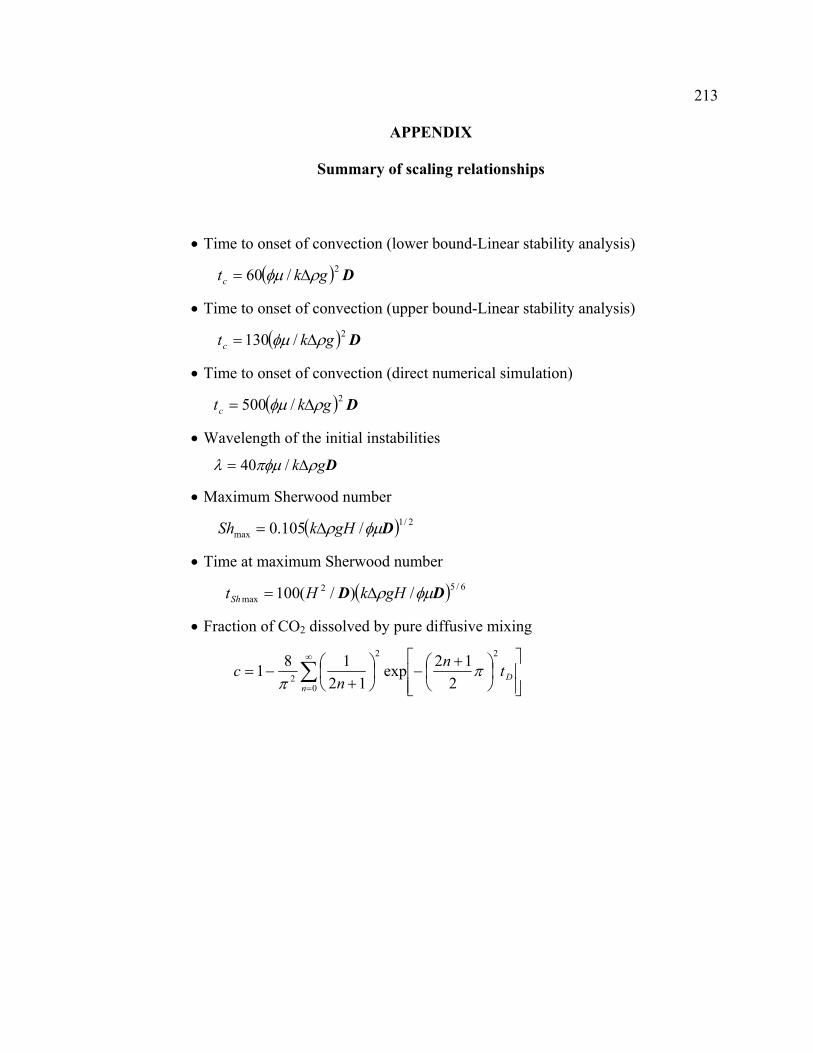


![Oktie Hassanzadeh Mariano Consens - Linked dataevents.linkeddata.org/ldow2009/slides/ldow2009-slides-hassanzadeh... · [Tutorial-VLDB05] Approximate Joins: Concepts and Techniques.](https://static.documents.pub/doc/80x56/5b3fe8497f8b9a3a138ca90d/oktie-hassanzadeh-mariano-consens-linked-tutorial-vldb05-approximate-joins.jpg)
