arX

iv:1

408.

1758

v1 [

astr

o-ph

.EP]

8 A

ug 2

014

Draft version August 11, 2014Preprint typeset using LATEX style emulateapj v. 5/2/11

HATS-6b: A WARM SATURN TRANSITING AN EARLY M DWARF STAR, AND A SET OF EMPIRICALRELATIONS FOR CHARACTERIZING K AND M DWARF PLANET HOSTS †

J. D. Hartman1, D. Bayliss2, R. Brahm3,4, G. A. Bakos1,⋆,⋆⋆, L. Mancini5, A. Jordan3,4, K. Penev1, M. Rabus3,5,G. Zhou2, R. P. Butler6, N. Espinoza3,4, M. de Val-Borro1, W. Bhatti1, Z. Csubry1, S. Ciceri5, T. Henning5,

B. Schmidt2, P. Arriagada6, S. Shectman7, J. Crane7, I. Thompson7, V. Suc3, B. Csak5, T. G. Tan8,R. W. Noyes9, J. Lazar10, I. Papp10, P. Sari10

Draft version August 11, 2014

ABSTRACT

We report the discovery by the HATSouth survey of HATS-6b, an extrasolar planet transiting aV=15.2mag, i = 13.7mag M1V star with a mass of 0.57M⊙ and a radius of 0.57R⊙. HATS-6b hasa period of P ≈ 3.3253d, mass of Mp ≈ 0.32MJ, radius of Rp ≈ 1.00RJ, and zero-albedo equilibriumtemperature of Teq = 712.8±5.1K. HATS-6 is one of the lowest mass stars known to host a close-in gasgiant planet, and its transits are among the deepest of any known transiting planet system. We discussthe follow-up opportunities afforded by this system, noting that despite the faintness of the host star,it is expected to have the highest K-band S/N transmission spectrum among known gas giant planetswith Teq < 750K. In order to characterize the star we present a new set of empirical relations betweenthe density, radius, mass, bolometric magnitude, and V , J , H and K-band bolometric corrections formain sequence stars with M < 0.80M⊙, or spectral types later than K5. These relations are calibratedusing eclipsing binary components as well as members of resolved binary systems. We account forintrinsic scatter in the relations in a self-consistent manner. We show that from the transit-basedstellar density alone it is possible to measure the mass and radius of a ∼ 0.6M⊙ star to ∼ 7% and∼ 2% precision, respectively. Incorporating additional information, such as the V − K color, or anabsolute magnitude, allows the precision to be improved by up to a factor of two.Subject headings: planetary systems — stars: individual (HATS-6) techniques: spectroscopic, photo-

metric

1. INTRODUCTION

One of the goals in the study of exoplanetary systemsis to determine how the properties of planets depend on

1 Department of Astrophysical Sciences, Princeton University,NJ 08544, USA; email: jhartman@astro.princeton.edu

2 The Australian National University, Canberra, Australia3 Instituto de Astrofısica, Facultad de Fısica, Pontificia Uni-

versidad Catolica de Chile, Av. Vicuna Mackenna 4860, 7820436Macul, Santiago, Chile

4 Millennium Institute of Astrophysics, Av. Vicuna Mackenna4860, 7820436 Macul, Santiago, Chile

5 Max Planck Institute for Astronomy, Heidelberg, Germany6 Department of Terrestrial Magnetism, Carnegie Institution

of Washington, 5241 Broad Branch Road NW, Washington, DC20015-1305, USA

7 The Observatories of the Carnegie Institution of Washing-ton, 813 Santa Barbara Street, Pasadena, CA 91101, USA

8 Perth Exoplanet Survey Telescope, Perth, Australia9 Harvard-Smithsonian Center for Astrophysics, Cambridge,

MA, USA10 Hungarian Astronomical Association, Budapest, Hungary⋆ Alfred P. Sloan Research Fellow⋆⋆ Packard Fellow† The HATSouth network is operated by a collaboration con-

sisting of Princeton University (PU), the Max Planck Insti-tute fur Astronomie (MPIA), the Australian National Univer-sity (ANU), and the Pontificia Universidad Catolica de Chile(PUC). The station at Las Campanas Observatory (LCO) of theCarnegie Institute is operated by PU in conjunction with PUC,the station at the High Energy Spectroscopic Survey (H.E.S.S.)site is operated in conjunction with MPIA, and the station atSiding Spring Observatory (SSO) is operated jointly with ANU.This paper includes data gathered with the 6.5 m Magellan Tele-scopes located as Las Campanas Observatory, Chile. Based inpart on observations made with the MPG 2.2 m Telescope andthe ESO 3.6 m Telescope at the ESO Observatory in La Silla.This paper uses observations obtained with facilities of the LasCumbres Observatory Global Telescope.

the properties of their host stars. An important parame-ter in this respect is the host star mass. Results fromboth radial velocity and transit surveys indicate thatthe occurrence rate of gas giant planets is a steep func-tion of stellar mass scaling approximately as N ∝ M⋆

(Johnson et al. 2010) for main sequence stars of type Mthrough F (smaller planets, on the other hand, appear tobe more frequent around M dwarfs than around hotterstars, Howard et al. 2012). The low occurrence rate ofthese planets around M dwarfs, coupled with the factthat most surveys primarily target FGK dwarf stars,means that only one hot Jupiter has so far been dis-covered around an M0 dwarf (Kepler-45; Johnson et al.2012), and only a handful of others have been foundaround very late K dwarf stars (WASP-80, Triaud et al.2013b; WASP-43, Hellier et al. 2011; and HAT-P-54,Bakos et al. 2014, being the only three known transiting-hot-Jupiter-hosting K dwarfs with M < 0.65M⊙).In addition to enabling the study of planetary proper-

ties as a function of stellar mass, finding planets aroundlate-type stars has at least two other advantages. Thesmall sizes of these stars coupled with their low luminosi-ties means that a planet with a given radius and orbitalperiod around a late-type star will produce deeper tran-sits and have a cooler equilibrium temperature than ifit were around a larger star. This makes planets aroundlate-type stars attractive targets for carrying out detailedfollow-up observations, such as atmospheric characteri-zations. A second, perhaps under appreciated, advan-tage of these stars is that they are remarkably simplein their bulk properties. Whereas, due to stellar evo-lution, the radius of a solar-metallicity, solar-mass star

2 Hartman et al.

varies by ∼ 40% over the 10Gyr age of the Galactic disk,the radius of a 0.6M⊙ star varies by less than ∼ 5%over the same time-span. The parameters of low-massstars follow tight main-sequence relations, enabling high-precision measurements of their properties from only asingle (or a few) observable(s). The precision of the stel-lar parameters feeds directly into the precision of theplanetary parameters, so that in principle planets aroundlow-mass stars may be characterized with higher preci-sion than those around higher mass stars.Here we present the discovery of a transiting, short-

period, gas-giant planet around an M1 dwarf star. Thisplanet, HATS-6b, was discovered by the HATSouth sur-vey, a global network of fully-automated wide-field pho-tometric instruments searching for transiting planets(Bakos et al. 2013). HATSouth uses larger-diameter op-tics than other similar projects allowing an enhanced sen-sitivity to faint K and M dwarfs.We also present a new set of empirical relations to use

in characterizing the properties of transiting planet hoststars with M < 0.80M⊙. While there has been muchdiscussion in the literature of the apparent discrepancybetween observations and various theoretical models forthese stars (e.g., Torres & Ribas 2002; Ribas 2003; Torres2013; Zhou et al. 2014, and references therein), the grow-ing set of well-characterized low-mass stars has revealedthat, as expected, these stars do follow tight main se-quence relations. We show that from the bulk density ofthe star alone, which is determined from the transit lightcurve and RV observations, it is possible to measure themass and radius of a ∼ 0.6M⊙ star to ∼ 7% and ∼ 2%precision, respectively. Incorporating additional infor-mation, such as the V −K color, or an absolute magni-tude, allows the precision to be improved by a factor oftwo.The layout of the paper is as follows. In Section 2 we

report the detection of the photometric signal and thefollow-up spectroscopic and photometric observations ofHATS-6. In Section 3 we describe the analysis of thedata, beginning with ruling out false positive scenarios,continuing with our global modelling of the photometryand radial velocities, and finishing with the determina-tion of the stellar parameters, and planetary parame-ters which depend on them, using both theoretical stellarmodels as well as the empirical relations which we derivehere. Our findings are discussed in Section 4.

2. OBSERVATIONS

2.1. Photometric detection

Observations of a field containing HATS-6 (see Ta-ble 9 for identifying information) were carried out withthe HS-2, HS-4 and HS-6 units of the HATSouth net-work (located at Las Campanas Observatory in Chile,the H.E.S.S. gamma-ray telescope site in Namibia, andSiding Spring Observatory in Australia, respectively; seeBakos et al. 2013 for a detailed description of the HAT-South network) between UT 2009-09-17 and UT 2010-09-10. A total 5695, 5544 and 88 images included in ourfinal trend and outlier-filtered light curves were obtainedwith HS-2, HS-4 and HS-6, respectively. Observationswere made through a Sloan r filter, using an exposuretime of 240 s and a median cadence of 293 s (see alsoTable 1).

-0.06

-0.04

-0.02

0

0.02

0.04

0.06

-0.4 -0.2 0 0.2 0.4

∆ m

ag

Orbital phase

-0.06

-0.04

-0.02

0

0.02

0.04

0.06

-0.06 -0.04 -0.02 0 0.02 0.04 0.06

∆ m

ag

Orbital phase

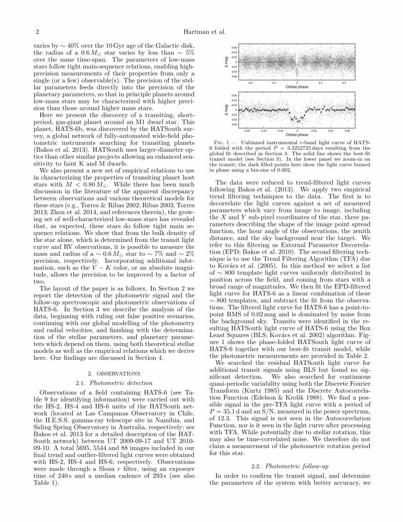
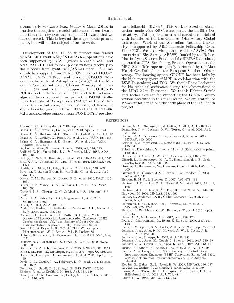
Fig. 1.— Unbinned instrumental r-band light curve of HATS-6 folded with the period P = 3.3252725 days resulting from theglobal fit described in Section 3. The solid line shows the best-fittransit model (see Section 3). In the lower panel we zoom-in onthe transit; the dark filled points here show the light curve binnedin phase using a bin-size of 0.002.

The data were reduced to trend-filtered light curvesfollowing Bakos et al. (2013). We apply two empiricaltrend filtering techniques to the data. The first is todecorrelate the light curves against a set of measuredparameters which vary from image to image, includingthe X and Y sub-pixel coordinates of the star, three pa-rameters describing the shape of the image point spreadfunction, the hour angle of the observations, the zenithdistance, and the sky background near the target. Werefer to this filtering as External Parameter Decorrela-tion (EPD; Bakos et al. 2010). The second filtering tech-nique is to use the Trend Filtering Algorithm (TFA) dueto Kovacs et al. (2005). In this method we select a listof ∼ 800 template light curves uniformly distributed inposition across the field, and coming from stars with abroad range of magnitudes. We then fit the EPD-filteredlight curve for HATS-6 as a linear combination of these∼ 800 templates, and subtract the fit from the observa-tions. The filtered light curve for HATS-6 has a point-to-point RMS of 0.02mag and is dominated by noise fromthe background sky. Transits were identified in the re-sulting HATSouth light curve of HATS-6 using the BoxLeast Squares (BLS; Kovacs et al. 2002) algorithm. Fig-ure 1 shows the phase-folded HATSouth light curve ofHATS-6 together with our best-fit transit model, whilethe photometric measurements are provided in Table 2.We searched the residual HATSouth light curve for

additional transit signals using BLS but found no sig-nificant detection. We also searched for continuousquasi-periodic variability using both the Discrete FourierTransform (Kurtz 1985) and the Discrete Autocorrela-tion Function (Edelson & Krolik 1988). We find a pos-sible signal in the pre-TFA light curve with a period ofP = 35.1 d and an S/N, measured in the power spectrum,of 12.3. This signal is not seen in the AutocorrelationFunction, nor is it seen in the light curve after processingwith TFA. While potentially due to stellar rotation, thismay also be time-correlated noise. We therefore do notclaim a measurement of the photometric rotation periodfor this star.

2.2. Photometric follow-up

In order to confirm the transit signal, and determinethe parameters of the system with better accuracy, we

HATS-6b 3

0

0.1

0.2

0.3

0.4

0.5

0.6-0.15 -0.1 -0.05 0 0.05 0.1 0.15

∆ (m

ag)

- A

rbitr

ary

offs

ets

Time from transit center (days)

RC-band

RC

RC

zs

i

z

RC

2013 Feb 17 - PEST

2013 Feb 27 - PEST

2013 Mar 29 - PEST

2013 Nov 23 - LCOGT 1m

2013 Dec 7 - LCOGT 1m

2012 Sep 3 - CTIO 0.9m

2013 Oct 27 - CTIO 0.9m

-0.1 -0.05 0 0.05 0.1

Time from transit center (days)

2013 Feb 17 - PEST

2013 Feb 27 - PEST

2013 Mar 29 - PEST

2013 Nov 23 - LCOGT 1m

2013 Dec 7 - LCOGT 1m

2012 Sep 3 - CTIO 0.9m

2013 Oct 27 - CTIO 0.9m

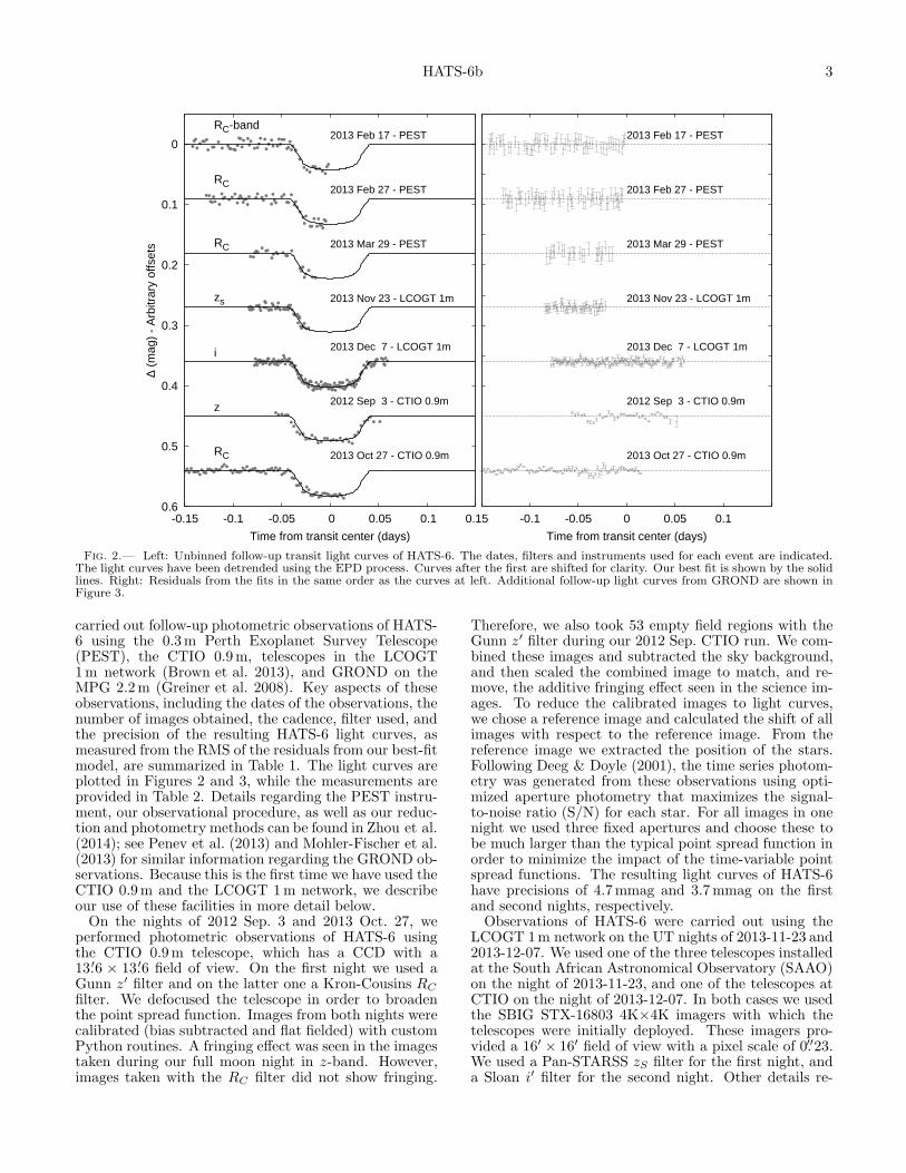
Fig. 2.— Left: Unbinned follow-up transit light curves of HATS-6. The dates, filters and instruments used for each event are indicated.The light curves have been detrended using the EPD process. Curves after the first are shifted for clarity. Our best fit is shown by the solidlines. Right: Residuals from the fits in the same order as the curves at left. Additional follow-up light curves from GROND are shown inFigure 3.

carried out follow-up photometric observations of HATS-6 using the 0.3m Perth Exoplanet Survey Telescope(PEST), the CTIO 0.9m, telescopes in the LCOGT1m network (Brown et al. 2013), and GROND on theMPG 2.2m (Greiner et al. 2008). Key aspects of theseobservations, including the dates of the observations, thenumber of images obtained, the cadence, filter used, andthe precision of the resulting HATS-6 light curves, asmeasured from the RMS of the residuals from our best-fitmodel, are summarized in Table 1. The light curves areplotted in Figures 2 and 3, while the measurements areprovided in Table 2. Details regarding the PEST instru-ment, our observational procedure, as well as our reduc-tion and photometry methods can be found in Zhou et al.(2014); see Penev et al. (2013) and Mohler-Fischer et al.(2013) for similar information regarding the GROND ob-servations. Because this is the first time we have used theCTIO 0.9m and the LCOGT 1m network, we describeour use of these facilities in more detail below.On the nights of 2012 Sep. 3 and 2013 Oct. 27, we

performed photometric observations of HATS-6 usingthe CTIO 0.9m telescope, which has a CCD with a13.′6 × 13.′6 field of view. On the first night we used aGunn z′ filter and on the latter one a Kron-Cousins RC

filter. We defocused the telescope in order to broadenthe point spread function. Images from both nights werecalibrated (bias subtracted and flat fielded) with customPython routines. A fringing effect was seen in the imagestaken during our full moon night in z-band. However,images taken with the RC filter did not show fringing.

Therefore, we also took 53 empty field regions with theGunn z′ filter during our 2012 Sep. CTIO run. We com-bined these images and subtracted the sky background,and then scaled the combined image to match, and re-move, the additive fringing effect seen in the science im-ages. To reduce the calibrated images to light curves,we chose a reference image and calculated the shift of allimages with respect to the reference image. From thereference image we extracted the position of the stars.Following Deeg & Doyle (2001), the time series photom-etry was generated from these observations using opti-mized aperture photometry that maximizes the signal-to-noise ratio (S/N) for each star. For all images in onenight we used three fixed apertures and choose these tobe much larger than the typical point spread function inorder to minimize the impact of the time-variable pointspread functions. The resulting light curves of HATS-6have precisions of 4.7mmag and 3.7mmag on the firstand second nights, respectively.Observations of HATS-6 were carried out using the

LCOGT 1m network on the UT nights of 2013-11-23 and2013-12-07. We used one of the three telescopes installedat the South African Astronomical Observatory (SAAO)on the night of 2013-11-23, and one of the telescopes atCTIO on the night of 2013-12-07. In both cases we usedthe SBIG STX-16803 4K×4K imagers with which thetelescopes were initially deployed. These imagers pro-vided a 16′ × 16′ field of view with a pixel scale of 0.′′23.We used a Pan-STARSS zS filter for the first night, anda Sloan i′ filter for the second night. Other details re-

4 Hartman et al.

0

0.01

0.02

0.03

0.04

0.05

0.06

0.07-0.1 -0.05 0 0.05 0.1

∆ (m

ag)

Time from transit center (days)

i-band

2014 Mar 6 - GROND/MPG 2.2m

-0.05 0 0.05 0.1

Time from transit center (days)

z-band

0

0.01

0.02

0.03

0.04

0.05

0.06

0.07

∆ (m

ag)

g-band r-band

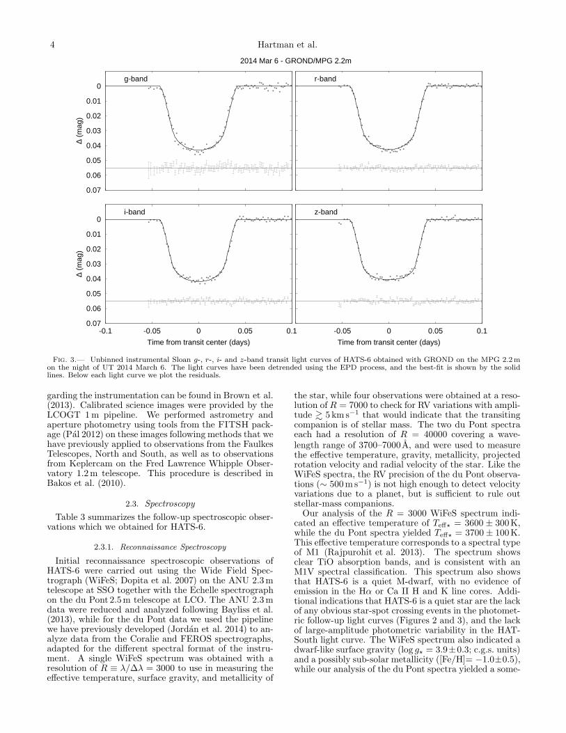
Fig. 3.— Unbinned instrumental Sloan g-, r-, i- and z-band transit light curves of HATS-6 obtained with GROND on the MPG 2.2 mon the night of UT 2014 March 6. The light curves have been detrended using the EPD process, and the best-fit is shown by the solidlines. Below each light curve we plot the residuals.

garding the instrumentation can be found in Brown et al.(2013). Calibrated science images were provided by theLCOGT 1m pipeline. We performed astrometry andaperture photometry using tools from the FITSH pack-age (Pal 2012) on these images following methods that wehave previously applied to observations from the FaulkesTelescopes, North and South, as well as to observationsfrom Keplercam on the Fred Lawrence Whipple Obser-vatory 1.2m telescope. This procedure is described inBakos et al. (2010).

2.3. Spectroscopy

Table 3 summarizes the follow-up spectroscopic obser-vations which we obtained for HATS-6.

2.3.1. Reconnaissance Spectroscopy

Initial reconnaissance spectroscopic observations ofHATS-6 were carried out using the Wide Field Spec-trograph (WiFeS; Dopita et al. 2007) on the ANU 2.3mtelescope at SSO together with the Echelle spectrographon the du Pont 2.5m telescope at LCO. The ANU 2.3mdata were reduced and analyzed following Bayliss et al.(2013), while for the du Pont data we used the pipelinewe have previously developed (Jordan et al. 2014) to an-alyze data from the Coralie and FEROS spectrographs,adapted for the different spectral format of the instru-ment. A single WiFeS spectrum was obtained with aresolution of R ≡ λ/∆λ = 3000 to use in measuring theeffective temperature, surface gravity, and metallicity of

the star, while four observations were obtained at a reso-lution of R = 7000 to check for RV variations with ampli-tude & 5 km s−1 that would indicate that the transitingcompanion is of stellar mass. The two du Pont spectraeach had a resolution of R = 40000 covering a wave-length range of 3700–7000A, and were used to measurethe effective temperature, gravity, metallicity, projectedrotation velocity and radial velocity of the star. Like theWiFeS spectra, the RV precision of the du Pont observa-tions (∼ 500m s−1) is not high enough to detect velocityvariations due to a planet, but is sufficient to rule outstellar-mass companions.Our analysis of the R = 3000 WiFeS spectrum indi-

cated an effective temperature of Teff⋆ = 3600 ± 300K,while the du Pont spectra yielded Teff⋆ = 3700± 100K.This effective temperature corresponds to a spectral typeof M1 (Rajpurohit et al. 2013). The spectrum showsclear TiO absorption bands, and is consistent with anM1V spectral classification. This spectrum also showsthat HATS-6 is a quiet M-dwarf, with no evidence ofemission in the Hα or Ca II H and K line cores. Addi-tional indications that HATS-6 is a quiet star are the lackof any obvious star-spot crossing events in the photomet-ric follow-up light curves (Figures 2 and 3), and the lackof large-amplitude photometric variability in the HAT-South light curve. The WiFeS spectrum also indicated adwarf-like surface gravity (log g⋆ = 3.9±0.3; c.g.s. units)and a possibly sub-solar metallicity ([Fe/H]= −1.0±0.5),while our analysis of the du Pont spectra yielded a some-

HATS-6b 5

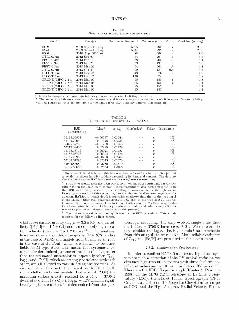
TABLE 1Summary of photometric observations

Facility Date(s) Number of Images a Cadence (s) b Filter Precision (mmag)

HS-2 2009 Sep–2010 Sep 5695 295 r 21.3HS-4 2009 Sep–2010 Sep 5544 293 r 21.0HS-6 2010 Aug–2010 Sep 88 296 r 18.6CTIO 0.9 m 2012 Sep 03 34 297 z 4.7PEST 0.3 m 2013 Feb 17 58 205 R 6.1PEST 0.3 m 2013 Feb 27 53 131 R 5.6PEST 0.3 m 2013 Mar 29 24 261 R 4.8CTIO 0.9 m 2013 Oct 27 99 181 RC 3.7LCOGT 1 m 2013 Nov 23 48 76 z 4.2LCOGT 1 m 2013 Dec 07 149 74 i 3.8GROND/MPG 2.2 m 2014 Mar 06 95 155 g 1.8GROND/MPG 2.2 m 2014 Mar 06 95 155 r 1.1GROND/MPG 2.2 m 2014 Mar 06 95 155 i 1.1GROND/MPG 2.2 m 2014 Mar 06 95 155 z 1.1

a Excludes images which were rejected as significant outliers in the fitting procedure.b The mode time difference rounded to the nearest second between consecutive points in each light curve. Due to visibility,weather, pauses for focusing, etc., none of the light curves have perfectly uniform time sampling.

TABLE 2Differential photometry of HATS-6

BJD Maga σMag Mag(orig)b Filter Instrument(2 400 000+)

55185.60957 −0.00387 0.01084 · · · r HS55145.70640 −0.07475 0.03251 · · · r HS55095.82750 −0.01258 0.01255 · · · r HS55275.39406 0.02245 0.01229 · · · r HS55195.58763 −0.00021 0.01587 · · · r HS55182.28728 0.00324 0.01174 · · · r HS55145.70968 −0.00768 0.02964 · · · r HS55185.61296 0.02073 0.01078 · · · r HS55095.83089 −0.02280 0.01379 · · · r HS55105.80688 −0.02863 0.02168 · · · r HS

Note. — This table is available in a machine-readable form in the online journal.A portion is shown here for guidance regarding its form and content. The data arealso available on the HATSouth website at http://www.hatsouth.org.a The out-of-transit level has been subtracted. For the HATSouth light curve (rowswith “HS” in the Instrument column), these magnitudes have been detrended usingthe EPD and TFA procedures prior to fitting a transit model to the light curve.Primarily as a result of this detrending, but also due to blending from neighbors, theapparent HATSouth transit depth is somewhat shallower than that of the true depthin the Sloan r filter (the apparent depth is 90% that of the true depth). For thefollow-up light curves (rows with an Instrument other than “HS”) these magnitudeshave been detrended with the EPD procedure, carried out simultaneously with thetransit fit (the transit shape is preserved in this process).b Raw magnitude values without application of the EPD procedure. This is onlyreported for the follow-up light curves.

what lower surface gravity (log g⋆ = 3.2±0.5) and metal-licity ([Fe/H]= −1.5± 0.5) and a moderately high rota-tion velocity (v sin i = 7.5 ± 2.0km s−1). The analysis,however, relies on synthetic templates (MARCS modelsin the case of WiFeS and models from Coelho et al. 2005in the case of du Pont) which are known to be unre-liable for M type stars. This means that systematic er-rors in the determined parameters are most likely greaterthan the estimated uncertainties (especially when Teff⋆,log g⋆ and [Fe/H], which are strongly correlated with eachother, are all allowed to vary in fitting the spectra). Asan example of this, note that based on the Dartmouthsingle stellar evolution models (Dotter et al. 2008) theminimum surface gravity realized for a Teff⋆ = 3700Kdwarf star within 13.8Gyr is log g⋆ = 4.73 which is signif-icantly higher than the values determined from the spec-

troscopic modelling (the only evolved single stars thatreach Teff⋆ = 3700K have log g⋆ . 2). We therefore donot consider the log g⋆ [Fe/H], or v sin i measurementsfrom this analysis to be reliable. More reliable estimateof Teff⋆ and [Fe/H] are presented in the next section.

2.3.2. Confirmation Spectroscopy

In order to confirm HATS-6 as a transiting planet sys-tem through a detection of the RV orbital variation weobtained high-resolution spectra with three facilities ca-pable of achieving ∼ 10m s−1 or better RV precision.These are the FEROS spectrograph (Kaufer & Pasquini1998) on the MPG 2.2m telescope at La Silla Obser-vatory (LSO), the Planet Finder Spectrograph (PFS;Crane et al. 2010) on the Magellan Clay 6.5m telescopeat LCO, and the High Accuracy Radial Velocity Planet

6 Hartman et al.

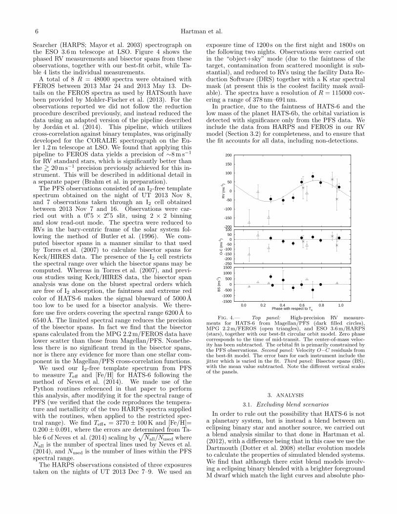
Searcher (HARPS; Mayor et al. 2003) spectrograph onthe ESO 3.6m telescope at LSO. Figure 4 shows thephased RV measurements and bisector spans from theseobservations, together with our best-fit orbit, while Ta-ble 4 lists the individual measurements.A total of 8 R = 48000 spectra were obtained with

FEROS between 2013 Mar 24 and 2013 May 13. De-tails on the FEROS spectra as used by HATSouth havebeen provided by Mohler-Fischer et al. (2013). For theobservations reported we did not follow the reductionprocedure described previously, and instead reduced thedata using an adapted version of the pipeline describedby Jordan et al. (2014). This pipeline, which utilizescross-correlation against binary templates, was originallydeveloped for the CORALIE spectrograph on the Eu-ler 1.2m telescope at LSO. We found that applying thispipeline to FEROS data yields a precision of ∼8m s−1

for RV standard stars, which is significantly better thanthe & 20m s−1 precision previously achieved for this in-strument. This will be described in additional detail ina separate paper (Brahm et al. in preparation).The PFS observations consisted of an I2-free template

spectrum obtained on the night of UT 2013 Nov 8,and 7 observations taken through an I2 cell obtainedbetween 2013 Nov 7 and 16. Observations were car-ried out with a 0.′′5 × 2.′′5 slit, using 2 × 2 binningand slow read-out mode. The spectra were reduced toRVs in the bary-centric frame of the solar system fol-lowing the method of Butler et al. (1996). We com-puted bisector spans in a manner similar to that usedby Torres et al. (2007) to calculate bisector spans forKeck/HIRES data. The presence of the I2 cell restrictsthe spectral range over which the bisector spans may becomputed. Whereas in Torres et al. (2007), and previ-ous studies using Keck/HIRES data, the bisector spananalysis was done on the bluest spectral orders whichare free of I2 absorption, the faintness and extreme redcolor of HATS-6 makes the signal blueward of 5000 Atoo low to be used for a bisector analysis. We there-fore use five orders covering the spectral range 6200 A to6540 A. The limited spectral range reduces the precisionof the bisector spans. In fact we find that the bisectorspans calculated from the MPG 2.2m/FEROS data havelower scatter than those from Magellan/PFS. Nonethe-less there is no significant trend in the bisector spans,nor is there any evidence for more than one stellar com-ponent in the Magellan/PFS cross-correlation functions.We used our I2-free template spectrum from PFS

to measure Teff and [Fe/H] for HATS-6 following themethod of Neves et al. (2014). We made use of thePython routines referenced in that paper to performthis analysis, after modifying it for the spectral range ofPFS (we verified that the code reproduces the tempera-ture and metallicity of the two HARPS spectra suppliedwith the routines, when applied to the restricted spec-tral range). We find Teff⋆ = 3770 ± 100K and [Fe/H]=0.200± 0.091, where the errors are determined from Ta-ble 6 of Neves et al. (2014) scaling by

√

Nall/Nused whereNall is the number of spectral lines used by Neves et al.(2014), and Nused is the number of lines within the PFSspectral range.The HARPS observations consisted of three exposures

taken on the nights of UT 2013 Dec 7–9. We used an

exposure time of 1200 s on the first night and 1800 s onthe following two nights. Observations were carried outin the “object+sky” mode (due to the faintness of thetarget, contamination from scattered moonlight is sub-stantial), and reduced to RVs using the facility Data Re-duction Software (DRS) together with a K star spectralmask (at present this is the coolest facility mask avail-able). The spectra have a resolution of R = 115000 cov-ering a range of 378 nm–691nm.In practice, due to the faintness of HATS-6 and the

low mass of the planet HATS-6b, the orbital variation isdetected with significance only from the PFS data. Weinclude the data from HARPS and FEROS in our RVmodel (Section 3.2) for completeness, and to ensure thatthe fit accounts for all data, including non-detections.

-200

-150

-100

-50

0

50

100

150

200

RV

(m

s-1)

-250-200-150-100

-50 0

50 100

O-C

(m

s-1)

-1500

-1000

-500

0

500

1000

1500

0.0 0.2 0.4 0.6 0.8 1.0

BS

(m

s-1)

Phase with respect to Tc

Fig. 4.— Top panel: High-precision RV measure-ments for HATS-6 from Magellan/PFS (dark filled circles),MPG 2.2 m/FEROS (open triangles), and ESO 3.6 m/HARPS(stars), together with our best-fit circular orbit model. Zero phasecorresponds to the time of mid-transit. The center-of-mass veloc-ity has been subtracted. The orbital fit is primarily constrained bythe PFS observations. Second panel: Velocity O−C residuals fromthe best-fit model. The error bars for each instrument include thejitter which is varied in the fit. Third panel: Bisector spans (BS),with the mean value subtracted. Note the different vertical scalesof the panels.

3. ANALYSIS

3.1. Excluding blend scenarios

In order to rule out the possibility that HATS-6 is nota planetary system, but is instead a blend between aneclipsing binary star and another source, we carried outa blend analysis similar to that done in Hartman et al.(2012), with a difference being that in this case we use theDartmouth (Dotter et al. 2008) stellar evolution modelsto calculate the properties of simulated blended systems.We find that although there exist blend models involv-ing a eclipsing binary blended with a brighter foregroundM dwarf which match the light curves and absolute pho-

HATS-6b 7

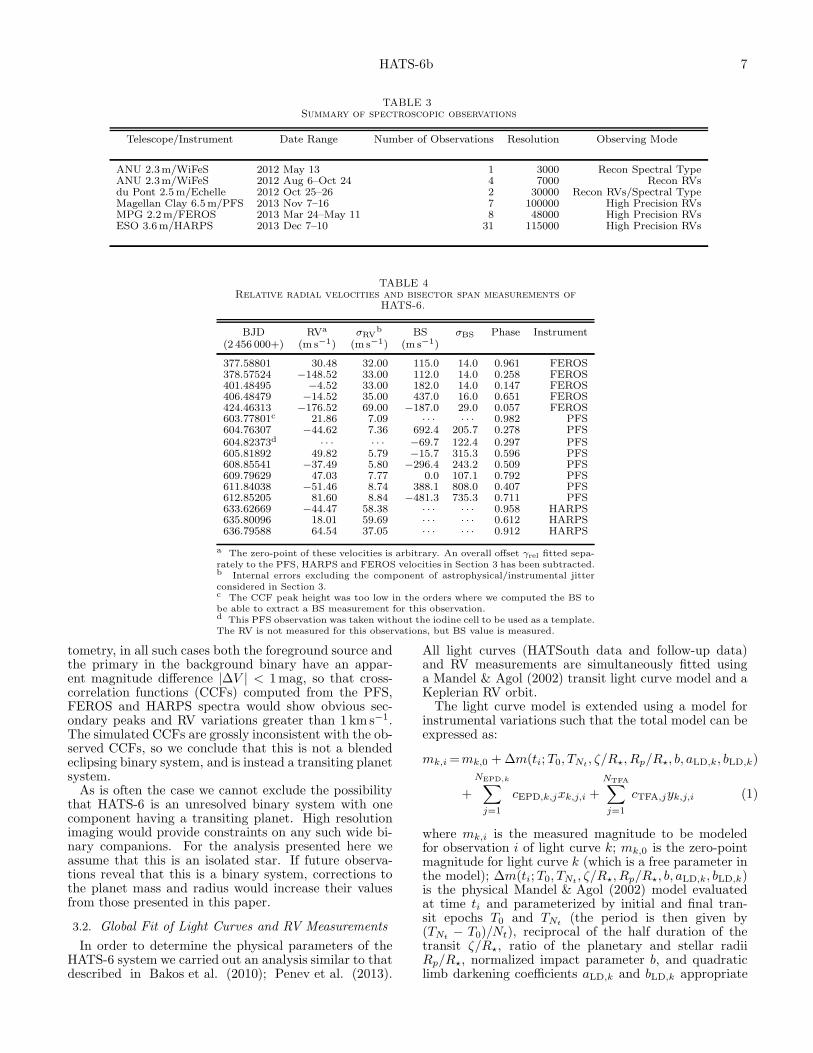
TABLE 3Summary of spectroscopic observations

Telescope/Instrument Date Range Number of Observations Resolution Observing Mode

ANU 2.3 m/WiFeS 2012 May 13 1 3000 Recon Spectral TypeANU 2.3 m/WiFeS 2012 Aug 6–Oct 24 4 7000 Recon RVsdu Pont 2.5 m/Echelle 2012 Oct 25–26 2 30000 Recon RVs/Spectral TypeMagellan Clay 6.5 m/PFS 2013 Nov 7–16 7 100000 High Precision RVsMPG 2.2 m/FEROS 2013 Mar 24–May 11 8 48000 High Precision RVsESO 3.6 m/HARPS 2013 Dec 7–10 31 115000 High Precision RVs

TABLE 4Relative radial velocities and bisector span measurements of

HATS-6.

BJD RVa σRVb BS σBS Phase Instrument

(2 456 000+) (m s−1) (m s−1) (m s−1)

377.58801 30.48 32.00 115.0 14.0 0.961 FEROS378.57524 −148.52 33.00 112.0 14.0 0.258 FEROS401.48495 −4.52 33.00 182.0 14.0 0.147 FEROS406.48479 −14.52 35.00 437.0 16.0 0.651 FEROS424.46313 −176.52 69.00 −187.0 29.0 0.057 FEROS603.77801c 21.86 7.09 · · · · · · 0.982 PFS604.76307 −44.62 7.36 692.4 205.7 0.278 PFS604.82373d · · · · · · −69.7 122.4 0.297 PFS605.81892 49.82 5.79 −15.7 315.3 0.596 PFS608.85541 −37.49 5.80 −296.4 243.2 0.509 PFS609.79629 47.03 7.77 0.0 107.1 0.792 PFS611.84038 −51.46 8.74 388.1 808.0 0.407 PFS612.85205 81.60 8.84 −481.3 735.3 0.711 PFS633.62669 −44.47 58.38 · · · · · · 0.958 HARPS635.80096 18.01 59.69 · · · · · · 0.612 HARPS636.79588 64.54 37.05 · · · · · · 0.912 HARPS

a The zero-point of these velocities is arbitrary. An overall offset γrel fitted sepa-rately to the PFS, HARPS and FEROS velocities in Section 3 has been subtracted.b Internal errors excluding the component of astrophysical/instrumental jitterconsidered in Section 3.c The CCF peak height was too low in the orders where we computed the BS tobe able to extract a BS measurement for this observation.d This PFS observation was taken without the iodine cell to be used as a template.The RV is not measured for this observations, but BS value is measured.

tometry, in all such cases both the foreground source andthe primary in the background binary have an appar-ent magnitude difference |∆V | < 1mag, so that cross-correlation functions (CCFs) computed from the PFS,FEROS and HARPS spectra would show obvious sec-ondary peaks and RV variations greater than 1 km s−1.The simulated CCFs are grossly inconsistent with the ob-served CCFs, so we conclude that this is not a blendedeclipsing binary system, and is instead a transiting planetsystem.As is often the case we cannot exclude the possibility

that HATS-6 is an unresolved binary system with onecomponent having a transiting planet. High resolutionimaging would provide constraints on any such wide bi-nary companions. For the analysis presented here weassume that this is an isolated star. If future observa-tions reveal that this is a binary system, corrections tothe planet mass and radius would increase their valuesfrom those presented in this paper.

3.2. Global Fit of Light Curves and RV Measurements

In order to determine the physical parameters of theHATS-6 system we carried out an analysis similar to thatdescribed in Bakos et al. (2010); Penev et al. (2013).

All light curves (HATSouth data and follow-up data)and RV measurements are simultaneously fitted usinga Mandel & Agol (2002) transit light curve model and aKeplerian RV orbit.The light curve model is extended using a model for

instrumental variations such that the total model can beexpressed as:

mk,i=mk,0 +∆m(ti;T0, TNt, ζ/R⋆, Rp/R⋆, b, aLD,k, bLD,k)

+

NEPD,k∑

j=1

cEPD,k,jxk,j,i +

NTFA∑

j=1

cTFA,jyk,j,i (1)

where mk,i is the measured magnitude to be modeledfor observation i of light curve k; mk,0 is the zero-pointmagnitude for light curve k (which is a free parameter inthe model); ∆m(ti;T0, TNt

, ζ/R⋆, Rp/R⋆, b, aLD,k, bLD,k)is the physical Mandel & Agol (2002) model evaluatedat time ti and parameterized by initial and final tran-sit epochs T0 and TNt

(the period is then given by(TNt

− T0)/Nt), reciprocal of the half duration of thetransit ζ/R⋆, ratio of the planetary and stellar radiiRp/R⋆, normalized impact parameter b, and quadraticlimb darkening coefficients aLD,k and bLD,k appropriate

8 Hartman et al.

for the filter of light curve k (except for aLD,k and bLD,k,which are fixed using the tabulations of Claret (2004),these parameters are varied in the fit); there are NEPD,k

EPD parameters applied to light curve k with cEPD,k,j

being the free coefficient fitted for EPD parameter seriesj applied to light curve k, and xk,j,i being the value ofEPD parameter series j at observation i for light curvek; and there are NTFA TFA templates used to fit thelight curve, with cTFA,j being the free coefficient fittedfor template j and yk,j,i being the value of template jat observation i for light curve k. For the HATSouthlight curve we do not include the EPD and TFA termsin the fit, and instead model the light curve that waspre-processed through these filtering routines without ac-counting for the transits. In this case we also includean instrumental blending factor (varied in the fit) whichscales the depth of the Mandel & Agol (2002) model ap-plied to the HATSouth light curve by a factor between0 and 1 (assuming a uniform prior between these limits)to account for both blending from nearby stars as wellas the artificial dilution of signals due to the filtering.For the RV model we allow an independent RV zero-

point, and an independent RV jitter for each of the threeinstruments used. The jitter is a term added in quadra-ture to the formal RV uncertainties for each instrumentand is varied in the fit following Hartman et al. (2012).We use a Differential Evolution Markov-Chain

Monte Carlo (DEMCMC) procedure (ter Braak 2006;Eastman et al. 2013) to explore the fitness of the modelover parameter space and produce a chain of parametersdrawn from the posterior distribution. This chain is thenused to estimate the most likely value (taken as the me-dian value over the chain) together with the 68.3% (1σ)confidence interval for each of the physical parameters.The fit is performed both allowing the eccentricity to

vary, and fixing it to zero. We find that without ad-ditional constraints, the free-eccentricity model stronglyprefers a non-zero eccentricity of e = 0.404± 0.058. Thisis entirely due to the PFS velocities which closely fol-low such an eccentric orbit with a near-zero jitter for thePFS RVs of 0.1±5.6m s−1. When the eccentricity is fixedto zero, on the other hand, the PFS RVs are consistentwith a circular orbit, but in this case require a jitter of26±14m s−1. Due to the faintness of HATS-6 in the opti-cal band-pass, and consequent sky contamination, such ahigh “jitter” is not unreasonable, and may simply reflectan underestimation of the formal RV uncertainties. Aswe discuss below, the stellar parameters inferred for thehigh eccentricity solution are inconsistent with the spec-troscopic parameters and broad-band photometric colorsof the star. When the photometric observations are di-rectly folded into our light curve and RV modelling, aswe discuss in Section 3.3.2, the preferred eccentricity isconsistent with zero (e = 0.053± 0.060).

3.3. Determining the Physical Parameters of the Starand Planet

To determine the mass and radius of the transitingplanet from the physical parameters measured above re-quires knowledge of the stellar mass and radius. Fora non-binary star such as HATS-6 these parameters arenot easy to measure directly and instead must be inferredby comparing other measurable parameters, such as thesurface temperature and bulk stellar density, with theo-

retical stellar evolution models (requiring the metallicity,a color indicator, and a luminosity indicator to identifya unique stellar model), or with empirical relations cali-brated using binary stars. We considered both methods,discussed in turn below.

3.3.1. Dartmouth Models

Because the star is a cool dwarf we make use ofthe Dartmouth stellar evolution models (Dotter et al.2008) which appear to provide the best match to Mdwarf and late K dwarf stars (e.g. Feiden et al. 2011;Sandquist et al. 2013). We also use the effective tem-perature and metallicity measured from the PFS I2-freetemplate spectrum.We use the results from our DEMCMC analysis of the

light curve and radial velocity data (Section 3.2) togetherwith the Dartmouth isochrones to determine the stel-lar parameters. For each density measurement in theposterior parameter chain we associate Teff and [Fe/H]measurements drawn from Gaussian distributions. Welook up a matching stellar model from the Dartmouthisochrones, interpolating between the tabulated models,and append the set of stellar parameters associated withthis model to the corresponding link in the posterior pa-rameter chain. Other planetary parameters, such as themass and radius, which depend on the stellar parametersare then calculated for each link in the chain.Figure 5 compares the measured Teff and ρ⋆ values

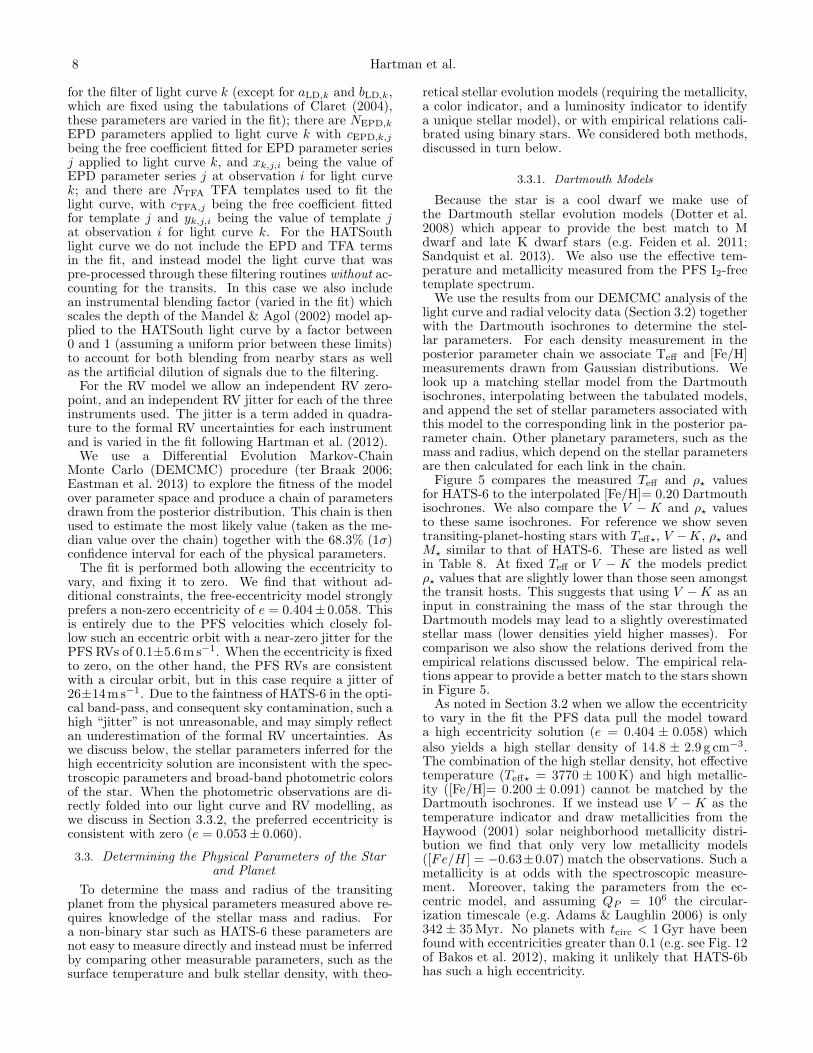
for HATS-6 to the interpolated [Fe/H]= 0.20 Dartmouthisochrones. We also compare the V − K and ρ⋆ valuesto these same isochrones. For reference we show seventransiting-planet-hosting stars with Teff⋆, V −K, ρ⋆ andM⋆ similar to that of HATS-6. These are listed as wellin Table 8. At fixed Teff or V − K the models predictρ⋆ values that are slightly lower than those seen amongstthe transit hosts. This suggests that using V −K as aninput in constraining the mass of the star through theDartmouth models may lead to a slightly overestimatedstellar mass (lower densities yield higher masses). Forcomparison we also show the relations derived from theempirical relations discussed below. The empirical rela-tions appear to provide a better match to the stars shownin Figure 5.As noted in Section 3.2 when we allow the eccentricity

to vary in the fit the PFS data pull the model towarda high eccentricity solution (e = 0.404 ± 0.058) whichalso yields a high stellar density of 14.8 ± 2.9 g cm−3.The combination of the high stellar density, hot effectivetemperature (Teff⋆ = 3770 ± 100K) and high metallic-ity ([Fe/H]= 0.200 ± 0.091) cannot be matched by theDartmouth isochrones. If we instead use V − K as thetemperature indicator and draw metallicities from theHaywood (2001) solar neighborhood metallicity distri-bution we find that only very low metallicity models([Fe/H ] = −0.63±0.07) match the observations. Such ametallicity is at odds with the spectroscopic measure-ment. Moreover, taking the parameters from the ec-centric model, and assuming QP = 106 the circular-ization timescale (e.g. Adams & Laughlin 2006) is only342 ± 35Myr. No planets with tcirc < 1Gyr have beenfound with eccentricities greater than 0.1 (e.g. see Fig. 12of Bakos et al. 2012), making it unlikely that HATS-6bhas such a high eccentricity.

HATS-6b 9

2.0

2.5

3.0

3.5

4.0

4.5

5.0

5.5

6.0

6.5340036003800400042004400

ρ * [g

/cm

3 ]

Effective temperature [K]2.0

2.5

3.0

3.5

4.0

4.5

5.0

5.5

6.0

6.5 3 3.2 3.4 3.6 3.8 4 4.2 4.4

ρ * [g

/cm

3 ]

V-K [mag]

0.50

0.52

0.54

0.56

0.58

0.60

0.62

0.64

0.66

0.68

0.70

3 3.2 3.4 3.6 3.8 4 4.2 4.4

M*

[Msu

n]

V-K [mag]

Fig. 5.— Model isochrones (dashed lines) from Dotter et al.(2008) for the spectroscopically determined metallicity of HATS-6and ages of 1 to 13 Gyr in 1 Gyr steps (showing ρ⋆ vs Teff at top,ρ⋆ vs V −K in the middle, and M⋆ vs V −K at the bottom). Themeasured values of Teff , V −K, and ρ⋆ for HATS-6, and the value ofM⋆ inferred from comparison to the stellar models, are shown usingthe large filled circles together with their 1σ and 2σ confidenceellipsoids. The open triangles show other transiting planet hoststars with measured Teff , V − K, ρ⋆ and M⋆ values similar toHATS-6. Near the K/M spectral type boundary (V −K ∼ 4) themodels predict somewhat lower densities for a given V −K or Teff

than are seen among transit hosts (Table 8). For comparison wealso show the relations derived from our empirical model (dottedlines; Section 3.3.2). In the top panel we show the three dotted linesare the median relation, and the 1σ lower and upper bounds. Inthe bottom two panels the lower dotted line is the median relation,while the upper dotted line is the 1σ upper bound. The 1σ lowerbound from the empirical model lies just outside the range of theseplots (below the bottom left corner in each case). The empiricalmodels appear to be more consistent with the transiting planethosts than the theoretical models, but also cover a broader rangeof parameter space than seen among the transit hosts.

3.3.2. Empirical Relations

As an alternative method to determine the stellar pa-rameters, and to better understand the degree of sys-tematic errors in these parameters, we also develop aset of empirical relations between stellar density, whichis directly measured for a transiting planet system, andother stellar parameters. Such relations have been devel-oped and employed in transiting exoplanet studies previ-ously (Torres et al. 2010; Enoch et al. 2010; Southworth2011). The Torres et al. (2010) and Enoch et al. (2010)relations only considered stars withM > 0.6M⊙, makingthem inapplicable in this case. The Southworth (2011)relations consider stars over the range 0.2M⊙ < M <3.0M⊙. They present two relations, one for mass asa function of temperature, density and metallicity, theother for radius as a function of temperature, densityand metallicity. Fitting these as two independent func-tions ignores the fact that density, mass, and radius mustsatisfy the relation M = 4

3πR3ρ. Moreover, one should

not expect the scaling of mass and radius with metal-licity or temperature to be independent of stellar massover such a broad range in mass. And, since metallicityis available for only very few M dwarf eclipsing binaries,the fit performed by Southworth (2011) effectively im-poses the metallicity scaling for A through G stars onthe M dwarfs. We therefore consider it worthwhile torevisit these relations for K and M dwarf stars.Johnson et al. (2011) and Johnson et al. (2012) have

also developed empirical relations for characterizing Mdwarf planet hosts, applying them to the characteriza-tion of LHS 6343 AB and Kepler-45, respectively. Ourapproach is similar to theirs in that we make use of re-lations between mass and absolute magnitudes based ondata from Delfosse et al. (2000), and we also consider theempirical mass–radius relation based on eclipsing bina-ries, however we differ in the sample of eclipsing binariesthat we consider, and we adopt a different parameter-ization of the problem. Moreover, while Johnson et al.(2012) use several empirical relations which were inde-pendently fit using different data sets, our approach isto self-consistently determine all of the relations througha joint analysis of the available data. We discuss thiscomparison in more detail below.We look for the following relations: (1) ρ⋆ → R⋆ (which

also defines a ρ⋆ → M⋆ relation), (2) M⋆ → Mbol, (whichtogether with relation 1 also defines a relation betweenTeff⋆ and the other parameters) (3) Teff⋆ → Mbol −MV ,(4) Teff⋆ → Mbol − MJ , (5) Teff⋆ → Mbol − MH , (6)Teff⋆ → Mbol − MK . The motivation for choosing thisparticular formulation is that ρ⋆ is typically a well-measured parameter for transiting planet systems, andthe relation between ρ⋆ and R⋆ is tighter than for otherrelations involving ρ⋆. The other relations are thenbased on physical dependencies (bolometric magnitudedepends primarily on stellar mass, with age and metal-licity being secondary factors, and bolometric correctionsdepend primarily on effective temperature, with metal-licity being a secondary factor). These relations are pa-rameterized as follows:

10 Hartman et al.

0.2

0.3

0.4

0.5

0.60.70.80.9

2 5 10 20 50

RS

tar/R

Sun

ρStar [g cm-3]

-0.2

-0.15

-0.1

-0.05

0

0.05

0.1

0.15

2 5 10 20 50

(∆R

Sta

r)/R

Sta

r

ρStar [g cm-3]

0.2

0.3

0.4

0.5

0.60.70.8

2 5 10 20 50

MS

tar/M

Sun

ρStar [g cm-3]

-0.2

-0.15

-0.1

-0.05

0

0.05

0.1

0.15

0.2

2 5 10 20 50

∆MS

tar/M

Sta

r

ρStar [g cm-3]

3

4

5

6

7

8

9

10

11

12

130.2 0.3 0.4 0.5 0.6 0.7 0.80.9

Mbo

l [m

ag]

MStar/MSun

-0.8

-0.6

-0.4

-0.2

0

0.2

0.4

0.6

0.80.2 0.3 0.4 0.5 0.6 0.7 0.80.9

∆Mbo

l [m

ag]

MStar/MSun

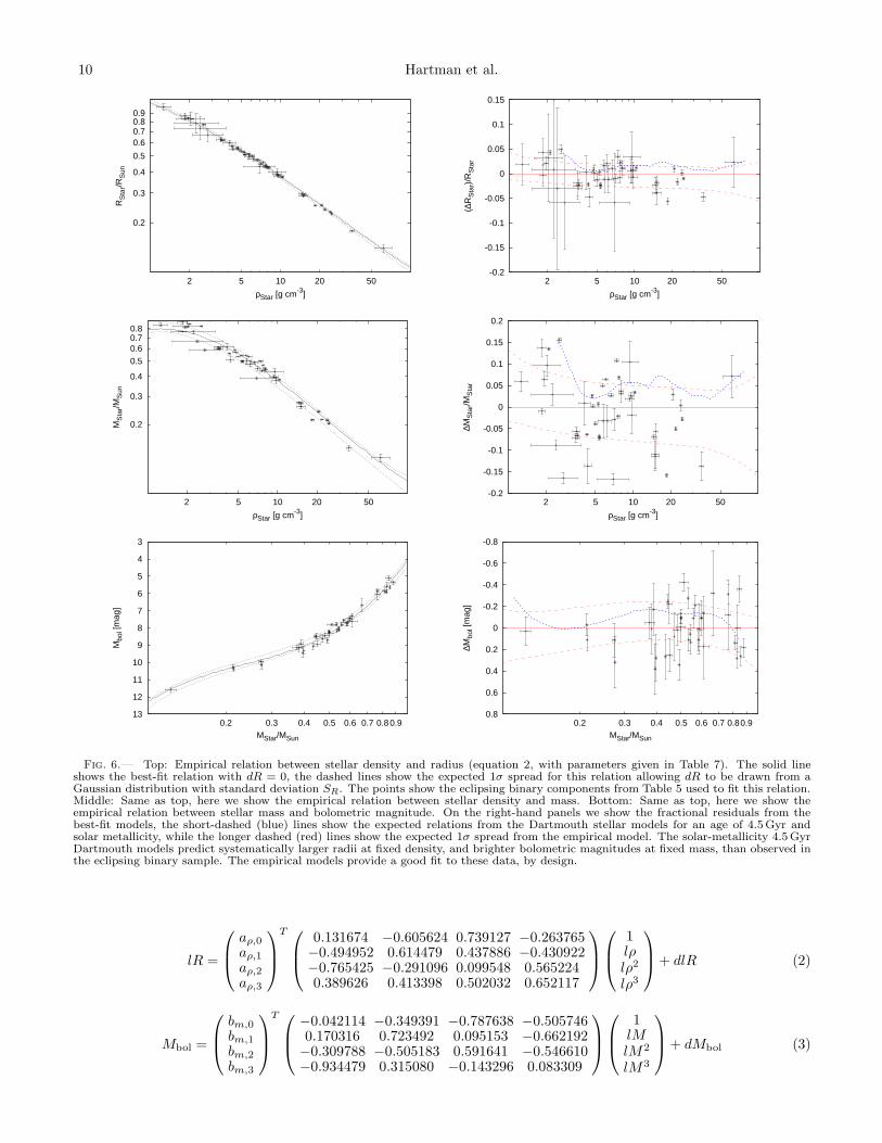
Fig. 6.— Top: Empirical relation between stellar density and radius (equation 2, with parameters given in Table 7). The solid lineshows the best-fit relation with dR = 0, the dashed lines show the expected 1σ spread for this relation allowing dR to be drawn from aGaussian distribution with standard deviation SR. The points show the eclipsing binary components from Table 5 used to fit this relation.Middle: Same as top, here we show the empirical relation between stellar density and mass. Bottom: Same as top, here we show theempirical relation between stellar mass and bolometric magnitude. On the right-hand panels we show the fractional residuals from thebest-fit models, the short-dashed (blue) lines show the expected relations from the Dartmouth stellar models for an age of 4.5 Gyr andsolar metallicity, while the longer dashed (red) lines show the expected 1σ spread from the empirical model. The solar-metallicity 4.5 GyrDartmouth models predict systematically larger radii at fixed density, and brighter bolometric magnitudes at fixed mass, than observed inthe eclipsing binary sample. The empirical models provide a good fit to these data, by design.

lR =

aρ,0aρ,1aρ,2aρ,3

T

0.131674 −0.605624 0.739127 −0.263765−0.494952 0.614479 0.437886 −0.430922−0.765425 −0.291096 0.099548 0.5652240.389626 0.413398 0.502032 0.652117

1lρlρ2

lρ3

+ dlR (2)

Mbol =

bm,0

bm,1

bm,2

bm,3

T

−0.042114 −0.349391 −0.787638 −0.5057460.170316 0.723492 0.095153 −0.662192−0.309788 −0.505183 0.591641 −0.546610−0.934479 0.315080 −0.143296 0.083309

1lMlM2

lM3

+ dMbol (3)

HATS-6b 11

-2

-1

0

1

2

3

4

5

6

7

2000 2500 3000 3500 4000 4500 5000 5500

MV -

Mbo

l [m

ag]

Τeff [K]

-3

-2.5

-2

-1.5

-1

-0.5

0

2000 2500 3000 3500 4000 4500 5000 5500

MJ

- M

bol [

mag

]

Τeff [K]

-3.4

-3.2

-3

-2.8

-2.6

-2.4

-2.2

-2

-1.8

-1.6

-1.4

2000 2500 3000 3500 4000 4500 5000 5500

MH

- M

bol [

mag

]

Τeff [K]

-4

-3.5

-3

-2.5

-2

-1.5

2000 2500 3000 3500 4000 4500 5000 5500

MK -

Mbo

l [m

ag]

Τeff [K]

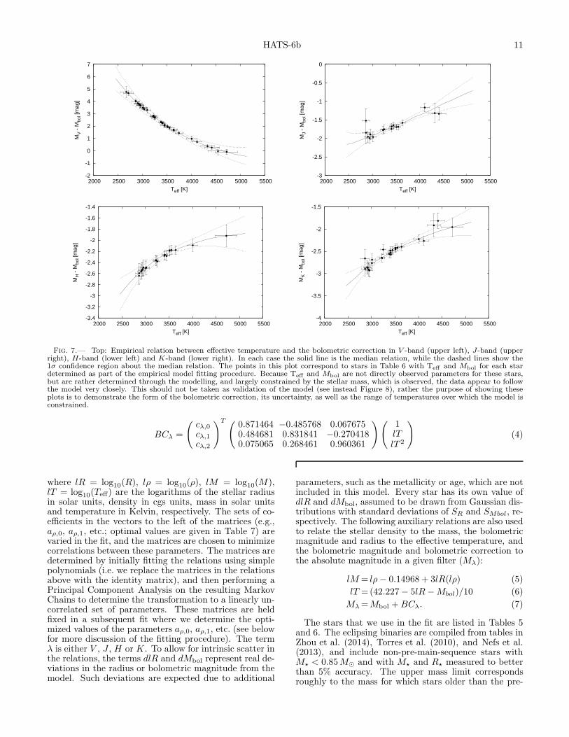
Fig. 7.— Top: Empirical relation between effective temperature and the bolometric correction in V -band (upper left), J-band (upperright), H-band (lower left) and K-band (lower right). In each case the solid line is the median relation, while the dashed lines show the1σ confidence region about the median relation. The points in this plot correspond to stars in Table 6 with Teff and Mbol for each stardetermined as part of the empirical model fitting procedure. Because Teff and Mbol are not directly observed parameters for these stars,but are rather determined through the modelling, and largely constrained by the stellar mass, which is observed, the data appear to followthe model very closely. This should not be taken as validation of the model (see instead Figure 8), rather the purpose of showing theseplots is to demonstrate the form of the bolometric correction, its uncertainty, as well as the range of temperatures over which the model isconstrained.

BCλ =

(

cλ,0cλ,1cλ,2

)T ( 0.871464 −0.485768 0.0676750.484681 0.831841 −0.2704180.075065 0.268461 0.960361

)(

1lTlT 2

)

(4)

where lR = log10(R), lρ = log10(ρ), lM = log10(M),lT = log10(Teff) are the logarithms of the stellar radiusin solar units, density in cgs units, mass in solar unitsand temperature in Kelvin, respectively. The sets of co-efficients in the vectors to the left of the matrices (e.g.,aρ,0, aρ,1, etc.; optimal values are given in Table 7) arevaried in the fit, and the matrices are chosen to minimizecorrelations between these parameters. The matrices aredetermined by initially fitting the relations using simplepolynomials (i.e. we replace the matrices in the relationsabove with the identity matrix), and then performing aPrincipal Component Analysis on the resulting MarkovChains to determine the transformation to a linearly un-correlated set of parameters. These matrices are heldfixed in a subsequent fit where we determine the opti-mized values of the parameters aρ,0, aρ,1, etc. (see belowfor more discussion of the fitting procedure). The termλ is either V , J , H or K. To allow for intrinsic scatter inthe relations, the terms dlR and dMbol represent real de-viations in the radius or bolometric magnitude from themodel. Such deviations are expected due to additional

parameters, such as the metallicity or age, which are notincluded in this model. Every star has its own value ofdlR and dMbol, assumed to be drawn from Gaussian dis-tributions with standard deviations of SR and SMbol, re-spectively. The following auxiliary relations are also usedto relate the stellar density to the mass, the bolometricmagnitude and radius to the effective temperature, andthe bolometric magnitude and bolometric correction tothe absolute magnitude in a given filter (Mλ):

lM = lρ− 0.14968 + 3lR(lρ) (5)

lT =(42.227− 5lR−Mbol)/10 (6)

Mλ=Mbol +BCλ. (7)

The stars that we use in the fit are listed in Tables 5and 6. The eclipsing binaries are compiled from tables inZhou et al. (2014), Torres et al. (2010), and Nefs et al.(2013), and include non-pre-main-sequence stars withM⋆ < 0.85M⊙ and with M⋆ and R⋆ measured to betterthan 5% accuracy. The upper mass limit correspondsroughly to the mass for which stars older than the pre-

12 Hartman et al.

0

2

4

6

8

10

12

14

16

18

0 0.1 0.2 0.3 0.4 0.5 0.6 0.7 0.8 0.9 1

MV [m

ag]

Mass [Msun]

3

4

5

6

7

8

9

10

11

0 0.1 0.2 0.3 0.4 0.5 0.6 0.7 0.8 0.9 1

MJ

[mag

]

Mass [Msun]

1

2

3

4

5

6

7

8

9

10

0 0.1 0.2 0.3 0.4 0.5 0.6 0.7 0.8 0.9 1

MH

[mag

]

Mass [Msun]

1

2

3

4

5

6

7

8

9

10

0 0.1 0.2 0.3 0.4 0.5 0.6 0.7 0.8 0.9 1

MK [m

ag]

Mass [Msun]

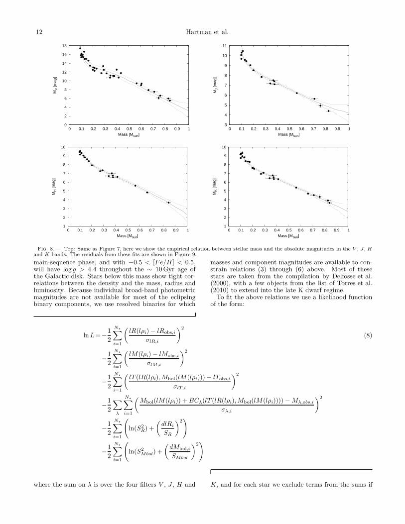
Fig. 8.— Top: Same as Figure 7, here we show the empirical relation between stellar mass and the absolute magnitudes in the V , J , Hand K bands. The residuals from these fits are shown in Figure 9.

main-sequence phase, and with −0.5 < [Fe/H ] < 0.5,will have log g > 4.4 throughout the ∼ 10Gyr age ofthe Galactic disk. Stars below this mass show tight cor-relations between the density and the mass, radius andluminosity. Because individual broad-band photometricmagnitudes are not available for most of the eclipsingbinary components, we use resolved binaries for which

masses and component magnitudes are available to con-strain relations (3) through (6) above. Most of thesestars are taken from the compilation by Delfosse et al.(2000), with a few objects from the list of Torres et al.(2010) to extend into the late K dwarf regime.To fit the above relations we use a likelihood function

of the form:

lnL=−1

2

N⋆∑

i=1

(

lR(lρi)− lRobs,i

σlR,i

)2

(8)

−1

2

N⋆∑

i=1

(

lM(lρi)− lMobs,i

σlM,i

)2

−1

2

N⋆∑

i=1

(

lT (lR(lρi),Mbol(lM(lρi)))− lTobs,i

σlT,i

)2

−1

2

∑

λ

N⋆∑

i=1

(

Mbol(lM(lρi)) +BCλ(lT (lR(lρi),Mbol(lM(lρi)))) −Mλ,obs,i

σλ,i

)2

−1

2

N⋆∑

i=1

(

ln(S2R) +

(

dlRi

SR

)2)

−1

2

N⋆∑

i=1

(

ln(S2Mbol) +

(

dMbol,i

SMbol

)2)

where the sum on λ is over the four filters V , J , H and K, and for each star we exclude terms from the sums if

HATS-6b 13

-2

-1.5

-1

-0.5

0

0.5

1

1.5

2

0 0.1 0.2 0.3 0.4 0.5 0.6 0.7 0.8 0.9 1

∆MV [m

ag]

Mass [Msun]

-1

-0.8

-0.6

-0.4

-0.2

0

0.2

0.4

0.6

0.8

1

0 0.1 0.2 0.3 0.4 0.5 0.6 0.7 0.8 0.9 1

∆MJ

[mag

]

Mass [Msun]

-1

-0.8

-0.6

-0.4

-0.2

0

0.2

0.4

0.6

0.8

1

0 0.1 0.2 0.3 0.4 0.5 0.6 0.7 0.8 0.9 1

∆MH

[mag

]

Mass [Msun]

-1

-0.8

-0.6

-0.4

-0.2

0

0.2

0.4

0.6

0.8

1

0 0.1 0.2 0.3 0.4 0.5 0.6 0.7 0.8 0.9 1

∆MK [m

ag]

Mass [Msun]

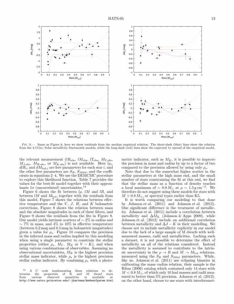
Fig. 9.— Same as Figure 8, here we show residuals from the median empirical relation. The short-dash (blue) lines show the relationfrom the 4.5 Gyr, Solar metallicity Dartmouth models, while the long-dash (red) lines show the expected 1σ spread of the empirical model.

the relevant measurement (lRobs, lMobs, lTobs, MV,obs,MJ,obs, MH,obs, or MK,obs) is not available. Here lρi,dlRi, and dMbol,i are free parameters for each star i, andthe other free parameters are SR, SMbol, and the coeffi-cients in equations 2–4. We use the DEMCMC procedureto explore this likelihood function. Table 7 provides thevalues for the best-fit model together with their approx-imate 1σ (uncorrelated) uncertainties.14

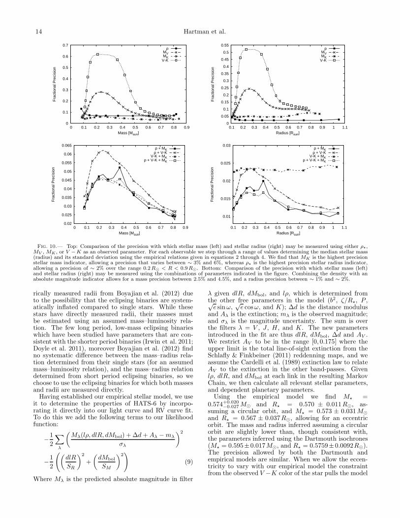
Figure 6 shows the fit between lρ, lM and lR, andbetween lM and Mbol, together with the residuals fromthis model, Figure 7 shows the relations between effec-tive temperature and the V , J , H , and K bolometriccorrections, Figure 8 shows the relation between massand the absolute magnitudes in each of these filters, andFigure 9 shows the residuals from the fits in Figure 8.Our model yields intrinsic scatters of ∼ 2% in radius and∼ 7% in mass, and 4% to 10% in effective temperature(between 0.2mag and 0.5mag in bolometric magnitudes)given a value for ρ⋆. Figure 10 compares the precisionin the inferred mass and radius implied by this modelingwhen using a single parameter to constrain the stellarproperties (either ρ⋆, MV , MK or V − K), and whenusing various combinations of observables. Assuming noobservational uncertainties, MK is the highest precisionstellar mass indicator, while ρ⋆ is the highest precisionstellar radius indicator. By combining ρ⋆ with a photo-

14 A C code implementing these relations to de-termine the properties of K and M dwarf starsfrom various observed quantities is available athttp://www.astro.princeton.edu/~jhartman/kmdwarfparam.html.

metric indicator, such as MK , it is possible to improvethe precision in mass and radius by up to a factor of twocompared to the precision allowed by using only ρ⋆.Note that due to the somewhat higher scatter in the

stellar parameters at the high mass end, and the smallnumber of stars constraining the fit at this end, we findthat the stellar mass as a function of density reachesa local maximum of ∼ 0.8M⊙ at ρ ∼ 1.5 g cm−3. Wetherefore do not suggest using these models for stars withM > 0.8M⊙, or spectral types earlier than K5.It is worth comparing our modeling to that done

by Johnson et al. (2011) and Johnson et al. (2012).One significant difference is the treatment of metallic-ity. Johnson et al. (2011) include a correlation betweenmetallicity and ∆MK (Johnson & Apps 2009), whileJohnson et al. (2012) include an additional correlationbetween metallicity and ∆J −K in their modelling. Wechoose not to include metallicity explicitly in our modeldue to the lack of a large sample of M dwarfs with well-measured masses, radii and metallicities. Lacking sucha dataset, it is not possible to determine the effect ofmetallicity on all of the relations considered. Insteadthe metallicity is assumed to contribute to the intrin-sic uncertainty in the ρ → R and M → Mbol relations,measured using the SR and SMbol parameters. While,like us, Johnson et al. (2011) use eclipsing binaries incalibrating the mass–radius relation, their sample is theRibas (2006) catalog which contained only 14 stars withM < 0.8M⊙, of which only 10 had masses and radii mea-sured to better than 5% precision. Johnson et al. (2012),on the other hand, choose to use stars with interferomet-

14 Hartman et al.

0

0.1

0.2

0.3

0.4

0.5

0.6

0.7

0 0.1 0.2 0.3 0.4 0.5 0.6 0.7 0.8 0.9

Fra

ctio

nal P

reci

sion

Mass [Msun]

ρMVMK

V-K

0

0.05

0.1

0.15

0.2

0.25

0.3

0.35

0.4

0.45

0.5

0.55

0.1 0.2 0.3 0.4 0.5 0.6 0.7 0.8 0.9 1 1.1

Fra

ctio

nal P

reci

sion

Radius [Rsun]

ρMVMK

V-K

0.02

0.025

0.03

0.035

0.04

0.045

0.05

0.055

0.06

0.065

0 0.1 0.2 0.3 0.4 0.5 0.6 0.7 0.8 0.9

Fra

ctio

nal P

reci

sion

Mass [Msun]

ρ + MKρ + V-K

V-K + MKρ + V-K + MK

0.01

0.015

0.02

0.025

0.03

0.1 0.2 0.3 0.4 0.5 0.6 0.7 0.8 0.9 1 1.1

Fra

ctio

nal P

reci

sion

Radius [Rsun]

ρ + MKρ + V-K

V-K + MKρ + V-K + MK

Fig. 10.— Top: Comparison of the precision with which stellar mass (left) and stellar radius (right) may be measured using either ρ⋆,MV , MK , or V −K as an observed parameter. For each observable we step through a range of values determining the median stellar mass(radius) and its standard deviation using the empirical relations given in equations 2 through 4. We find that MK is the highest precisionstellar mass indicator, allowing a precision that varies between ∼ 3% and 6%, whereas ρ⋆ is the highest precision stellar radius indicator,allowing a precision of ∼ 2% over the range 0.2R⊙ < R < 0.9R⊙. Bottom: Comparison of the precision with which stellar mass (left)and stellar radius (right) may be measured using the combinations of parameters indicated in the figure. Combining the density with anabsolute magnitude indicator allows for a mass precision between 2.5% and 4.5%, and a radius precision between ∼ 1% and ∼ 2%.

rically measured radii from Boyajian et al. (2012) dueto the possibility that the eclipsing binaries are system-atically inflated compared to single stars. While thesestars have directly measured radii, their masses mustbe estimated using an assumed mass–luminosity rela-tion. The few long period, low-mass eclipsing binarieswhich have been studied have parameters that are con-sistent with the shorter period binaries (Irwin et al. 2011;Doyle et al. 2011), moreover Boyajian et al. (2012) findno systematic difference between the mass–radius rela-tion determined from their single stars (for an assumedmass–luminosity relation), and the mass–radius relationdetermined from short period eclipsing binaries, so wechoose to use the eclipsing binaries for which both massesand radii are measured directly.Having established our empirical stellar model, we use

it to determine the properties of HATS-6 by incorpo-rating it directly into our light curve and RV curve fit.To do this we add the following terms to our likelihoodfunction:

−1

2

∑

λ

(

Mλ(lρ, dlR, dMbol) + ∆d+Aλ −mλ

σλ

)2

−1

2

(

(

dlR

SR

)2

+

(

dMbol

SM

)2)

(9)

Where Mλ is the predicted absolute magnitude in filter

λ given dlR, dMbol, and lρ, which is determined fromthe other free parameters in the model (b2, ζ/R⋆, P ,√e sinω,

√e cosω, and K); ∆d is the distance modulus

and Aλ is the extinction; mλ is the observed magnitude;and σλ is the magnitude uncertainty. The sum is overthe filters λ = V , J , H , and K. The new parametersintroduced in the fit are thus dlR, dMbol, ∆d and AV .We restrict AV to be in the range [0, 0.175] where theupper limit is the total line-of-sight extinction from theSchlafly & Finkbeiner (2011) reddenning maps, and weassume the Cardelli et al. (1989) extinction law to relateAV to the extinction in the other band-passes. Givenlρ, dlR, and dMbol at each link in the resulting MarkovChain, we then calculate all relevant stellar parameters,and dependent planetary parameters.Using the empirical model we find M⋆ =

0.574+0.020−0.027 M⊙ and R⋆ = 0.570 ± 0.011R⊙, as-

suming a circular orbit, and M⋆ = 0.573 ± 0.031M⊙and R⋆ = 0.567 ± 0.037R⊙, allowing for an eccentricorbit. The mass and radius inferred assuming a circularorbit are slightly lower than, though consistent with,the parameters inferred using the Dartmouth isochrones(M⋆ = 0.595± 0.017M⊙, and R⋆ = 0.5759± 0.0092R⊙).The precision allowed by both the Dartmouth andempirical models are similar. When we allow the eccen-tricity to vary with our empirical model the constraintfrom the observed V −K color of the star pulls the model

HATS-6b 15

TABLE 5K and M Dwarf Binary Components Used to Fit Empirical Relations a

Star Mass Radius Teff Reference(M⊙) (R⊙) (K)

1 RXS J154727.5+450803 A 0.2576 ± 0.0085 0.2895 ± 0.0068 . . . 11 RXS J154727.5+450803 B 0.2585 ± 0.0080 0.2895 ± 0.0068 . . . 1ASA J011328–3821.1 A 0.612 ± 0.03 0.596 ± 0.02 3750 ± 250 2CG Cyg B 0.814 ± 0.013 0.838 ± 0.011 4720 ± 60 3,4CM Dra A 0.2130 ± 0.0009 0.2534 ± 0.0019 3130 ± 70 5CM Dra B 0.2141 ± 0.0010 0.2396 ± 0.0015 3120 ± 70 5CU Cnc A 0.4333 ± 0.0017 0.4317 ± 0.0052 3160 ± 150 6CU Cnc B 0.3980 ± 0.0014 0.3908 ± 0.0094 3130 ± 150 6GJ 3236 A 0.376 ± 0.016 0.3795 ± 0.0084 3310 ± 110 7GJ 551 b 0.123 ± 0.006 0.141 ± 0.007 3098 ± 56 8,9,10GU Boo A 0.610 ± 0.006 0.627 ± 0.016 3920 ± 130 11GU Boo B 0.600 ± 0.006 0.624 ± 0.016 3810 ± 130 11HATS550-016 0.110+0.005

−0.006 0.147+0.003−0.004 . . . 12

HATS551-021 0.132+0.014−0.005 0.154+0.006

−0.008 . . . 12HD 195987 A 0.844 ± 0.018 0.98 ± 0.04 5200 ± 100 13J1219-39 B 0.091 ± 0.002 0.1174+0.0071

−0.0050 . . . 14

Kepler-16 B 0.20255+0.00066−0.00065 0.22623+0.00059

−0.00055 . . . 15

KIC 1571511 B 0.14136+0.0051−0.0042 0.17831+0.0013

−0.0016 . . . 16KOI-126 B 0.2413 ± 0.0030 0.2543 ± 0.0014 . . . 17KOI-126 C 0.2127 ± 0.0026 0.2318 ± 0.0013 . . . 17LSPM J1112+7626 A 0.3946 ± 0.0023 0.3860 ± 0.0055 3060 ± 160 18LSPM J1112+7626 B 0.2745 ± 0.0012 0.2978 ± 0.0049 2950 ± 160 18MG1-116309 A 0.567 ± 0.002 0.552 ± 0.0085 3920 ± 80 19MG1-116309 B 0.532 ± 0.002 0.532 ± 0.006 3810 ± 80 19MG1-1819499 A 0.557 ± 0.001 0.569 ± 0.0022 3690 ± 80 19MG1-1819499 B 0.535 ± 0.001 0.500 ± 0.0085 3610 ± 80 19MG1-2056316 A 0.4690 ± 0.0021 0.441 ± 0.002 3460 ± 180 19MG1-2056316 B 0.382 ± 0.001 0.374 ± 0.002 3320 ± 180 19MG1-506664 A 0.584 ± 0.002 0.560 ± 0.0025 3730 ± 90 19MG1-506664 B 0.544 ± 0.002 0.513 ± 0.0055 3610 ± 90 19MG1 646680A 0.499 ± 0.002 0.457 ± 0.006 3730 ± 50 19MG1-646680 B 0.443 ± 0.002 0.427 ± 0.006 3630 ± 50 19MG1-78457 B 0.491 ± 0.002 0.471 ± 0.009 3270 ± 100 19NSVS 01031772 A 0.5428 ± 0.0027 0.526 ± 0.0028 3615 ± 72 20NSVS 01031772 B 0.4982 ± 0.0025 0.5087 ± 0.0031 3520 ± 30 20NSVS 6550671 A 0.510 ± 0.02 0.550 ± 0.01 3730 ± 60 21T-Cyg1-01385 B 0.43 ± 0.02 0.40 ± 0.02 . . . 22UV Psc B 0.7644 ± 0.0045 0.835 ± 0.018 4750 ± 80 23V568 Lyr B 0.8273 ± 0.0042 0.7679 ± 0.0064 4900 ± 100 24WOCS 23009 B 0.447 ± 0.011 0.4292 ± 0.0033 3620 ± 150 25WTS19b-2-01387 A 0.498 ± 0.019 0.496 ± 0.013 3498 ± 100 26WTS19b-2-01387 B 0.481 ± 0.017 0.479 ± 0.013 3436 ± 100 26YY Gem A 0.599 ± 0.005 0.619 ± 0.006 3819 ± 98 27YY Gem B 0.599 ± 0.005 0.619 ± 0.006 3819 ± 98 27

References. — 1: Hartman et al. (2011); 2: He lminiak et al. (2012); 3: Bedford et al. (1987); 4:Popper (1994); 5: Morales et al. (2009); 6: Ribas (2003); 7: Irwin et al. (2009); 8: Segransan et al.(2003); 9: Valenti & Fischer (2005); 10: Demory et al. (2009); 11: Lopez-Morales & Ribas (2005);12: Zhou et al. (2014); 13: Torres et al. (2002); 14: Triaud et al. (2013a); 15: Doyle et al. (2011);16: Ofir et al. (2012); 17: Carter et al. (2011); 18: Irwin et al. (2011); 19: Kraus et al. (2011); 20:Lopez-Morales et al. (2006); 21: Dimitrov & Kjurkchieva (2010); 22: Fernandez et al. (2009); 23:Popper (1997); 24: Grundahl et al. (2008); 25: Sandquist et al. (2013); 26: Birkby et al. (2012);27: Torres & Ribas (2002)a Data compiled primarily from tables given in Torres et al. (2010), Nefs et al. (2013) andZhou et al. (2014), we provide the original references for each source in the table.b This is a single star, with an interferometric radius measurement, and mass estimated assuminga mass-luminosity relation.

to a lower eccentricity solution, yielding parameters thatare consistent with those from the fixed-circular model.For the final parameters we suggest adopting those fromthe empirical stellar model, assuming a circular orbit.The adopted stellar parameters are listed in Table 9while the planetary parameters are listed in Table 10.

4. DISCUSSION

In this paper we have presented the discovery of theHATS-6 transiting planet system by the HATSouth sur-vey. We found that HATS-6b has a mass of 0.319 ±

0.070MJ, radius of 0.998 ± 0.019RJ and orbits a starwith a mass of 0.574+0.020

−0.027 M⊙. HATS-6 is one of onlyfour stars with M . 0.6M⊙ known to host a short periodgas giant planet (the other three are WASP-80, WASP-43, and Kepler-45; see Table 8). This is illustrated inFigure 11 where we plot planet mass against the hoststar mass. We note that the published masses for thesestars come from a disparate set of methods. Apply-ing the empirical relations developed in this paper (Sec-tion 3.3.2) to these two systems, using ρ⋆, V , J , H and

16 Hartman et al.

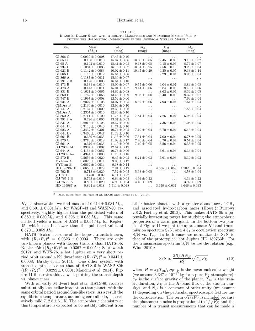
TABLE 6K and M Dwarf Stars with Absolute Magnitudes and Measured Masses Used in

Fitting the Bolometric Corrections in the Empirical Stellar Model a

Star Mass MV MJ MH MK

(M⊙) (mag) (mag) (mag) (mag)

Gl 866 C 0.0930 ± 0.0008 17.43 ± 0.40 . . . . . . . . .Gl 65 B 0.100 ± 0.010 15.87 ± 0.06 10.06 ± 0.05 9.45 ± 0.03 9.16 ± 0.07Gl 65 A 0.102 ± 0.010 15.41 ± 0.05 9.68 ± 0.05 9.15 ± 0.03 8.76 ± 0.07Gl 234 B 0.1034 ± 0.0035 16.16 ± 0.07 10.31 ± 0.25 9.56 ± 0.10 9.26 ± 0.04Gl 623 B 0.1142 ± 0.0083 16.02 ± 0.11 10.47 ± 0.29 9.35 ± 0.05 9.33 ± 0.14Gl 866 B 0.1145 ± 0.0012 15.64 ± 0.08 . . . 9.29 ± 0.04 8.96 ± 0.04Gl 866 A 0.1187 ± 0.0011 15.39 ± 0.07 . . . . . . . . .Gl 791.2 B 0.126 ± 0.003 16.64 ± 0.10 . . . . . . . . .Gl 473 B 0.131 ± 0.010 15.00 ± 0.07 9.57 ± 0.06 9.04 ± 0.07 8.84 ± 0.08Gl 473 A 0.143 ± 0.011 15.01 ± 0.07 9.44 ± 0.06 8.84 ± 0.06 8.40 ± 0.06Gl 831 B 0.1621 ± 0.0065 14.62 ± 0.08 . . . 8.62 ± 0.05 8.36 ± 0.05Gl 860 B 0.1762 ± 0.0066 13.46 ± 0.09 9.03 ± 0.08 8.40 ± 0.05 8.32 ± 0.07Gl 747 B 0.1997 ± 0.0008 12.52 ± 0.06 . . . . . . 7.63 ± 0.04Gl 234 A 0.2027 ± 0.0106 13.07 ± 0.05 8.52 ± 0.06 7.93 ± 0.04 7.64 ± 0.04CMDra B 0.2136 ± 0.0010 12.94 ± 0.10 . . . . . . . . .Gl 747 A 0.2137 ± 0.0009 12.30 ± 0.06 . . . . . . 7.53 ± 0.04CMDra A 0.2307 ± 0.0010 12.80 ± 0.10 . . . . . . . . .Gl 860 A 0.2711 ± 0.0100 11.76 ± 0.05 7.84 ± 0.04 7.26 ± 0.04 6.95 ± 0.04Gl 791.2 A 0.286 ± 0.006 13.37 ± 0.03 . . . . . . . . .Gl 831 A 0.2913 ± 0.0125 12.52 ± 0.06 . . . 7.36 ± 0.05 7.08 ± 0.05Gl 644 Bb 0.3143 ± 0.0040 11.71 ± 0.10 . . . . . . . . .Gl 623 A 0.3432 ± 0.0301 10.74 ± 0.05 7.19 ± 0.04 6.70 ± 0.04 6.46 ± 0.04Gl 644 Ba 0.3466 ± 0.0047 11.22 ± 0.10 . . . . . . . . .Gl 661 B 0.369 ± 0.035 11.15 ± 0.06 7.51 ± 0.04 7.02 ± 0.04 6.78 ± 0.05Gl 570 C 0.3770 ± 0.0018 11.09 ± 0.17 7.40 ± 0.04 6.76 ± 0.04 6.57 ± 0.04Gl 661 A 0.379 ± 0.035 11.10 ± 0.06 7.10 ± 0.05 6.56 ± 0.04 6.36 ± 0.05GJ 2069 Ab 0.3987 ± 0.0007 12.57 ± 0.19 . . . . . . . . .Gl 644 A 0.4155 ± 0.0057 10.76 ± 0.06 . . . 6.61 ± 0.05 6.35 ± 0.04GJ 2069 Aa 0.4344 ± 0.0008 11.78 ± 0.18 . . . . . . . . .Gl 570 B 0.5656 ± 0.0029 9.45 ± 0.05 6.21 ± 0.03 5.61 ± 0.03 5.39 ± 0.03YYGem A 0.6028 ± 0.0014 9.03 ± 0.12 . . . . . . . . .YYGem B 0.6069 ± 0.0014 9.38 ± 0.14 . . . . . . . . .HD 195987 B 0.6650 ± 0.0079 7.91 ± 0.19 . . . 4.835 ± 0.059 4.702 ± 0.034Gl 702 B 0.713 ± 0.029 7.52 ± 0.05 5.63 ± 0.05 . . . 4.53 ± 0.04χ Dra B 0.750 ± 0.02 6.11 ± 0.27 . . . . . . . . .GJ 765.2 B 0.763 ± 0.019 6.64 ± 0.05 4.94 ± 0.22 . . . 4.34 ± 0.22GJ 765.2 A 0.831 ± 0.020 5.99 ± 0.04 4.40 ± 0.09 . . . 3.92 ± 0.09HD 195987 A 0.844 ± 0.018 5.511 ± 0.028 . . . 3.679 ± 0.037 3.646 ± 0.033

a Data taken from Delfosse et al. (2000) and Torres et al. (2010).

KS as observables, we find masses of 0.614± 0.031M⊙,and 0.601± 0.031M⊙, for WASP-43 and WASP-80, re-spectively, slightly higher than the published values of0.580 ± 0.050M⊙ and 0.596 ± 0.035M⊙. This samemethod yields a mass of 0.534 ± 0.034M⊙ for Kepler-45, which is a bit lower than the published value of0.570± 0.059M⊙.HATS-6b also has some of the deepest transits known,

with (Rp/R⋆)2 = 0.0323 ± 0.0003. There are only

two known planets with deeper transits than HATS-6b:Kepler-45b ((Rp/R⋆)

2 = 0.0362 ± 0.0054; Southworth2012), and WTS-2b, a hot Jupiter on a very short pe-riod orbit around a K2 dwarf star ((Rp/R⋆)

2 = 0.0347±0.0008; Birkby et al. 2014). One other system withtransit depths close to that of HATS-6 is WASP-80b((Rp/R⋆)

2 = 0.0292± 0.0001; Mancini et al. 2014). Fig-ure 11 illustrates this as well, plotting the transit depthvs. planet mass.With an early M dwarf host star, HATS-6b receives

substantially less stellar irradiation than planets with thesame orbital period around Sun-like stars. As a result theequilibrium temperature, assuming zero albedo, is a rel-atively mild 712.8±5.1K. The atmospheric chemistry atthis temperature is expected to be notably different from

other hotter planets, with a greater abundance of CH4

and associated hydro-carbon hazes (Howe & Burrows2012; Fortney et al. 2013). This makes HATS-6b a po-tentially interesting target for studying the atmosphericproperties of a warm gas giant. In the bottom two pan-els of Figure 11 we plot the approximate K-band trans-mission spectrum S/N, and 4.5µm occultation spectrumS/N vs. Teq. In both cases we normalize the S/N tothat of the prototypical hot Jupiter HD 189733b. Forthe transmission spectrum S/N we use the relation (e.g.,Winn 2010):

S/N ∝ 2RPHNH

R2⋆

√

T14FK (10)

where H = kBTeq/µgP , µ is the mean molecular weight(we assume 3.347× 10−27 kg for a pure H2 atmosphere),gP is the surface gravity of the planet, T14 is the tran-sit duration, FK is the K-band flux of the star in Jan-skys, and NH is a constant of order unity (we assume1) depending on the particular spectroscopic feature un-der consideration. The term

√T14FK is included because

the photometric noise is proportional to 1/√FK and the

number of in transit measurements that can be made is

HATS-6b 17

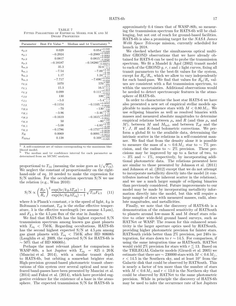
TABLE 7Fitted Parameters of Empirical Model for K and M

Dwarf Properties

Parameter Best Fit Value a Median and 1σ Uncertainty b

aρ,0 0.029 0.054+0.048−0.049

aρ,1 −0.2924 −0.2989+0.0083−0.0084

aρ,2 0.0817 0.0815+0.0020−0.0020

aρ,3 −0.18187 −0.18280+0.00075−0.00074

bm,0 35.3 32.6+3.1−3.3

bm,1 −7.54 −7.09+0.44−0.44

bm,2 1.17 1.24+0.10−0.11

bm,3 −7.717 −7.690+0.034−0.034

cV,0 1070 570+380−370

cV,1 15.3 16.5+2.2−2.9

cV,2 0.099 0.111+0.013−0.013

cJ,0 130 100+150−190

cJ,1 −5.0 −5.4+1.2−1.1

cJ,2 −0.1154 −0.1105+0.0043−0.0046

cH,0 −70 −130+150−140

cH,1 −3.96 −3.46+0.96−1.13

cH,2 −0.1619 −0.1615+0.0044−0.0041

cK,0 50 −80+140−140

cK,1 −5.08 −4.83+0.92−0.99

cK,2 −0.1786 −0.1757+0.0039−0.0038

SR 0.0069 0.0091+0.0010−0.0012

SMbol 0.138 0.169+0.022−0.025

a A self-consistent set of values corresponding to the maximum like-lihood model.b The median and 1σ confidence interval for each parameter asdetermined from an MCMC analysis.

proportional to T14 (meaning the noise goes as 1/√T14).

We neglect the constant of proportionality on the right-hand-side of eq. 10 needed to make the expression forS/N unitless. For the occultation spectrum S/N we usethe relation (e.g., Winn 2010):

S/N ∝(

RP

R⋆

)2exp(hc/kBλTeff)− 1

exp(hc/kBλTeq)− 1

√

T14F4.5 (11)

where h is Planck’s constant, c is the speed of light, kB isBoltmann’s constant, Teff is the stellar effective temper-ature, λ is the effective wavelength (we assume 4.5µm),and F4.5 is the 4.5µm flux of the star in Janskys.We find that HATS-6b has the highest expected S/N

transmission spectrum among known gas giant planetswith Teq < 750K. Regarding occultations, HATS-6bhas the second highest expected S/N at 4.5µm amonggas giant planets with Teq < 750K after HD 80606b(Laughlin et al. 2009, the expected S/N for HATS-6b is∼ 50% that of HD 80606b).Perhaps the most relevant planet for comparison is

WASP-80b, a hot Jupiter with Teq = 825 ± 20K(Mancini et al. 2014), with a similar transit depthto HATS-6b, but orbiting a somewhat brighter star.High-precision ground-based photometric transit obser-vations of this system over several optical and near in-frared band-passes have been presented by Mancini et al.(2014) and Fukui et al. (2014), which have provided sug-gestive evidence for the existence of a haze in the atmo-sphere. The expected transmission S/N for HATS-6b is

approximately 0.4 times that of WASP-80b, so measur-ing the transmission spectrum for HATS-6b will be chal-lenging, but not out of reach for ground-based facilities.HATS-6b is also a promising target for the NASA JamesWebb Space Telescope mission, currently scheduled forlaunch in 2018.We checked whether the simultaneous optical multi-

filter GROND observations that we have already ob-tained for HATS-6 can be used to probe the transmissionspectrum. We fit a Mandel & Agol (2002) transit modelto each of the GROND g, r, i and z light curves, fixing alltransit parameters to the best-fit values for the system,except for Rp/R⋆, which we allow to vary independentlyfor each band-pass. We find that values for Rp/R⋆ val-ues are consistent with a flat transmission spectrum, towithin the uncertainties. Additional observations wouldbe needed to detect spectroscopic features in the atmo-sphere of HATS-6b.In order to characterize the host star HATS-6 we have

also presented a new set of empirical stellar models ap-plicable to main-sequence stars with M < 0.80M⊙. Weuse eclipsing binaries as well as resolved binaries withmasses and measured absolute magnitudes to determineempirical relations between ρ⋆ and R (and thus ρ⋆ andM), between M and Mbol, and between Teff and theV , J , H and K-band bolometric corrections. We per-form a global fit to the available data, determining theintrinsic scatter in the relations in a self-consistent man-ner. We find that from the density alone it is possibleto measure the mass of a ∼ 0.6M⊙ star to ∼ 7% pre-cision, and the radius to ∼ 2% precision. These pre-cisions may be improved by up to a factor of two, to∼ 3% and ∼ 1%, respectively, by incorporating addi-tional photometric data. The relations presented hereare similar to those presented by Johnson et al. (2011)and Johnson et al. (2012) except that we do not attemptto incorporate metallicity directly into the model (it con-tributes instead to the inherent scatter in the relations),and we use a much larger sample of eclipsing binariesthan previously considered. Future improvements to ourmodel may be made by incorporating metallicity infor-mation directly into the model, but this will require alarge sample of stars with measured masses, radii, abso-lute magnitudes, and metallicities.Finally, we note that the discovery of HATS-6b is a

demonstration of the enhanced sensitivity of HATSouthto planets around low-mass K and M dwarf stars rela-tive to other wide-field ground based surveys, such asHATNet or WASP. The reason for this enhanced sensi-tivity is the larger aperture optics used by HATSouth,providing higher photometric precision for fainter stars.HATSouth yields better than 2% precision, per 240 s in-tegration, for stars down to r ∼ 14.5. For comparison, ifusing the same integration time as HATSouth, HATNetwould yield 2% precision for stars with r . 13. Based onthe TRILEGAL Galactic models (Girardi et al. 2005) weestimate that there are∼ 230000 stars withM < 0.6M⊙,r < 14.5 in the Southern sky, and at least 10◦ from theGalactic disk that could be observed by HATSouth. Thisis nearly a factor of ten more than the number of starswith M < 0.6M⊙ and r < 13.0 in the Northern sky thatcould be observed by HATNet to the same photometricprecision. While in principle the discovery of HATS-6bmay be used to infer the occurrence rate of hot Jupiters

18 Hartman et al.

TABLE 8Transiting-planet hosting stars with similar properties to HATS-6.

Star Mass Radius V −K ρ⋆ Planet Mass Planet Period ReferenceM⊙ R⊙ mag g cm−3 MJ day

GJ 3470 0.541 ± 0.067 0.503 ± 0.063 4.281 ± 0.030 6.0 ± 2.4 0.0441 ± 0.0053 3.34 1WASP-80 0.596 ± 0.035 0.593 ± 0.012 3.53 ± 0.23 4.040 ± 0.012 0.562 ± 0.027 3.07 2,8KIC 10905746 0.578 ± 0.032 0.548 ± 0.026 3.94 ± 0.24 4.97 ± 0.54 . . . 9.88 3WASP-43 0.580 ± 0.050 0.598+0.034

−0.042 3.212 ± 0.027 3.81+0.86−0.51 1.78 ± 0.10 0.81 4

Kepler-45 0.570 ± 0.059 0.539 ± 0.039 3.990 ± 0.058 5.12 ± 0.73 0.500 ± 0.061 2.46 5,9HAT-P-54 0.645 ± 0.020 0.617 ± 0.013 3.179 ± 0.063 3.88 ± 0.27 0.760 ± 0.032 3.80 6Kepler-26 0.650 ± 0.030 0.590 ± 0.030 3.352 ± 0.026 4.47 ± 0.71 . . . a 12.28 7

References. — 1: Bonfils et al. (2012); 2: Triaud et al. (2013b); 3: Fischer et al. (2012); 4: Hellier et al. (2011); 5: Johnson et al.(2012); 6: Bakos et al. (2014); 7: Steffen et al. (2012); 8: Mancini et al. (2014); 9: Southworth (2012)a The period listed is for Kepler-26b, the innermost of the four planets transiting this star.

TABLE 9Stellar parameters for HATS-6

Parameter Value Isochrones a Value Empirical b Value Empirical b

Circ. Circ. Eccen.

Identifying Information

R.A. (h:m:s; 2MASS) 05h52m35.22s . . . . . .Dec. (d:m:s; 2MASS) −19◦01′54.0′′ . . . . . .2MASS ID 2MASS 05523523-1901539 . . . . . .

Spectroscopic properties c

Teff⋆ (K) . . . . . . . . . . . . 3770 ± 100 . . . . . .[Fe/H] . . . . . . . . . . . . . . 0.200 ± 0.091 . . . . . .

Photometric properties

B (mag; APASS). . . . 16.664 ± 0.043 . . . . . .V (mag; APASS). . . . 15.160 ± 0.024 . . . . . .J (mag; 2MASS) . . . . 12.046 ± 0.024 . . . . . .H (mag; 2MASS) . . . 11.397 ± 0.023 . . . . . .Ks (mag; 2MASS) . . 11.224 ± 0.023 . . . . . .

Derived properties

M⋆ (M⊙) . . . . . . . . . . . 0.595 ± 0.017 0.574+0.020−0.027 0.573 ± 0.031

R⋆ (R⊙) . . . . . . . . . . . . 0.5759 ± 0.0092 0.570 ± 0.011 0.567 ± 0.037Teff⋆ (K) d . . . . . . . . . . 3872 ± 53 3724 ± 18 3722 ± 19ρ⋆ (cgs) . . . . . . . . . . . . . 4.40 ± 0.13 4.36 ± 0.15 4.42+0.75

−0.47log g⋆ (cgs) . . . . . . . . . . 4.6920 ± 0.0077 4.683 ± 0.010 4.689 ± 0.038L⋆ (L⊙) . . . . . . . . . . . . 0.0670 ± 0.0054 0.0558 ± 0.0024 0.0555 ± 0.0073MV (mag) . . . . . . . . . . 9.43 ± 0.19 9.209 ± 0.075 9.22 ± 0.15MK (mag,ESO) . . . . . 5.079 ± 0.065 5.387 ± 0.043 5.40 ± 0.14Age (Gyr). . . . . . . . . . . 8.1 ± 4.3 . . . . . .Distance (pc) . . . . . . . 172.6 ± 5.5 148.4 ± 3.3 147.8+7.0

−9.4

a Parameters based on combining the bulk stellar density determined from our fit to the light curves andRV data for HATS-6, the effective temperature and metallicity from the Magellan/PFS spectrum, togetherwith the Dartmouth (Dotter et al. 2008) stellar evolution models. We perform the fit two ways: allowingthe eccentricity to vary (Eccen.), and keeping it fixed to zero (Circ.). The estimated value for ρ⋆ differssignificantly between these two fits. For the eccentric orbit fit the stellar density cannot be reproduced bythe Dartmouth models given the measured effective temperature and metallicity. We therefore only listthe parameters based on the Dartmouth models for the circular orbit fit.b Parameters based on our empirical relations for K and M dwarf stellar properties, which are includeddirectly in our global modelling of the light curves and RV data for HATS-6. Again we perform thefit two ways: allowing the eccentricity to vary, and keeping it fixed to zero. In this case including theconstraint from the observed V − K color of the star directly in the RV and light-curve modelling pullsthe free-eccentricity model to a lower eccentricity solution, yielding stellar parameters that are consistentwith those from the fixed-circular model.c These parameters are determined from the I2-free Magellan/PFS spectrum of HATS-6 using the methodof Neves et al. (2014).d The effective temperature listed here is derived from the Dartmouth stellar models, or from ourempirical stellar relations, and is not measured directly from the spectrum.

HATS-6b 19

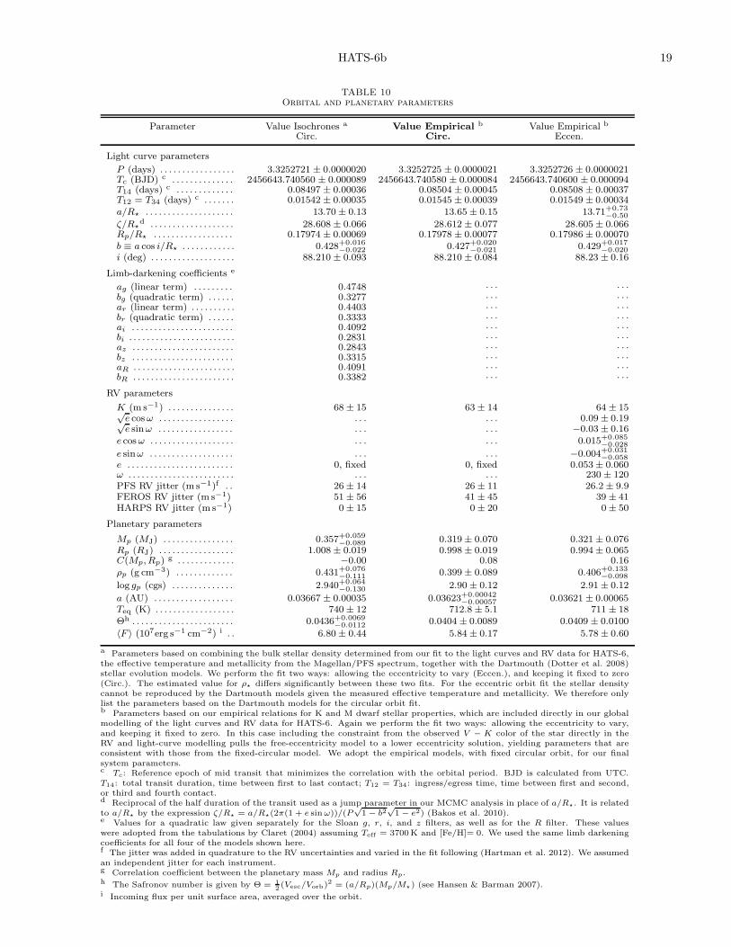
TABLE 10Orbital and planetary parameters

Parameter Value Isochrones a Value Empirical b Value Empirical b

Circ. Circ. Eccen.

Light curve parameters

P (days) . . . . . . . . . . . . . . . . . 3.3252721 ± 0.0000020 3.3252725 ± 0.0000021 3.3252726 ± 0.0000021Tc (BJD) c . . . . . . . . . . . . . . 2456643.740560 ± 0.000089 2456643.740580 ± 0.000084 2456643.740600 ± 0.000094T14 (days) c . . . . . . . . . . . . . 0.08497 ± 0.00036 0.08504 ± 0.00045 0.08508 ± 0.00037T12 = T34 (days) c . . . . . . . 0.01542 ± 0.00035 0.01545 ± 0.00039 0.01549 ± 0.00034a/R⋆ . . . . . . . . . . . . . . . . . . . . 13.70 ± 0.13 13.65 ± 0.15 13.71+0.73

−0.50

ζ/R⋆d . . . . . . . . . . . . . . . . . . . 28.608 ± 0.066 28.612 ± 0.077 28.605 ± 0.066

Rp/R⋆ . . . . . . . . . . . . . . . . . . 0.17974 ± 0.00069 0.17978 ± 0.00077 0.17986 ± 0.00070b ≡ a cos i/R⋆ . . . . . . . . . . . . 0.428+0.016

−0.022 0.427+0.020−0.021 0.429+0.017

−0.020i (deg) . . . . . . . . . . . . . . . . . . . 88.210 ± 0.093 88.210 ± 0.084 88.23 ± 0.16

Limb-darkening coefficients e

ag (linear term) . . . . . . . . . 0.4748 · · · · · ·bg (quadratic term) . . . . . . 0.3277 · · · · · ·ar (linear term) . . . . . . . . . . 0.4403 · · · · · ·br (quadratic term) . . . . . . 0.3333 · · · · · ·ai . . . . . . . . . . . . . . . . . . . . . . . 0.4092 · · · · · ·bi . . . . . . . . . . . . . . . . . . . . . . . . 0.2831 · · · · · ·az . . . . . . . . . . . . . . . . . . . . . . . 0.2843 · · · · · ·bz . . . . . . . . . . . . . . . . . . . . . . . 0.3315 · · · · · ·aR . . . . . . . . . . . . . . . . . . . . . . . 0.4091 · · · · · ·bR . . . . . . . . . . . . . . . . . . . . . . . 0.3382 · · · · · ·

RV parameters

K (m s−1) . . . . . . . . . . . . . . . 68 ± 15 63 ± 14 64 ± 15√e cosω . . . . . . . . . . . . . . . . . . . . . . . 0.09 ± 0.19√e sinω . . . . . . . . . . . . . . . . . . . . . . . −0.03 ± 0.16

e cosω . . . . . . . . . . . . . . . . . . . . . . . . . 0.015+0.085−0.028

e sinω . . . . . . . . . . . . . . . . . . . . . . . . . −0.004+0.031−0.058

e . . . . . . . . . . . . . . . . . . . . . . . . 0, fixed 0, fixed 0.053 ± 0.060ω . . . . . . . . . . . . . . . . . . . . . . . . . . . . . . 230 ± 120PFS RV jitter (m s−1)f . . 26 ± 14 26 ± 11 26.2 ± 9.9FEROS RV jitter (m s−1) 51 ± 56 41 ± 45 39 ± 41HARPS RV jitter (m s−1) 0 ± 15 0 ± 20 0 ± 50

Planetary parameters

Mp (MJ) . . . . . . . . . . . . . . . . 0.357+0.059−0.089 0.319 ± 0.070 0.321 ± 0.076

Rp (RJ) . . . . . . . . . . . . . . . . . 1.008 ± 0.019 0.998 ± 0.019 0.994 ± 0.065C(Mp, Rp) g . . . . . . . . . . . . . −0.00 0.08 0.16ρp (g cm−3) . . . . . . . . . . . . . 0.431+0.076

−0.111 0.399 ± 0.089 0.406+0.133−0.098

log gp (cgs) . . . . . . . . . . . . . . 2.940+0.064−0.130 2.90 ± 0.12 2.91 ± 0.12

a (AU) . . . . . . . . . . . . . . . . . . 0.03667 ± 0.00035 0.03623+0.00042−0.00057 0.03621 ± 0.00065

Teq (K) . . . . . . . . . . . . . . . . . . 740 ± 12 712.8 ± 5.1 711 ± 18Θh . . . . . . . . . . . . . . . . . . . . . . . 0.0436+0.0069

−0.0112 0.0404 ± 0.0089 0.0409 ± 0.0100

〈F 〉 (107erg s−1 cm−2) i . . 6.80 ± 0.44 5.84 ± 0.17 5.78 ± 0.60

a Parameters based on combining the bulk stellar density determined from our fit to the light curves and RV data for HATS-6,the effective temperature and metallicity from the Magellan/PFS spectrum, together with the Dartmouth (Dotter et al. 2008)stellar evolution models. We perform the fit two ways: allowing the eccentricity to vary (Eccen.), and keeping it fixed to zero(Circ.). The estimated value for ρ⋆ differs significantly between these two fits. For the eccentric orbit fit the stellar densitycannot be reproduced by the Dartmouth models given the measured effective temperature and metallicity. We therefore onlylist the parameters based on the Dartmouth models for the circular orbit fit.b Parameters based on our empirical relations for K and M dwarf stellar properties, which are included directly in our globalmodelling of the light curves and RV data for HATS-6. Again we perform the fit two ways: allowing the eccentricity to vary,and keeping it fixed to zero. In this case including the constraint from the observed V − K color of the star directly in theRV and light-curve modelling pulls the free-eccentricity model to a lower eccentricity solution, yielding parameters that areconsistent with those from the fixed-circular model. We adopt the empirical models, with fixed circular orbit, for our finalsystem parameters.c Tc: Reference epoch of mid transit that minimizes the correlation with the orbital period. BJD is calculated from UTC.T14: total transit duration, time between first to last contact; T12 = T34: ingress/egress time, time between first and second,or third and fourth contact.d Reciprocal of the half duration of the transit used as a jump parameter in our MCMC analysis in place of a/R⋆. It is relatedto a/R⋆ by the expression ζ/R⋆ = a/R⋆(2π(1 + e sinω))/(P

√1 − b2

√1 − e2) (Bakos et al. 2010).

e Values for a quadratic law given separately for the Sloan g, r, i, and z filters, as well as for the R filter. These valueswere adopted from the tabulations by Claret (2004) assuming Teff = 3700 K and [Fe/H]= 0. We used the same limb darkeningcoefficients for all four of the models shown here.f The jitter was added in quadrature to the RV uncertainties and varied in the fit following (Hartman et al. 2012). We assumedan independent jitter for each instrument.g Correlation coefficient between the planetary mass Mp and radius Rp.h The Safronov number is given by Θ = 1

2(Vesc/Vorb)2 = (a/Rp)(Mp/M⋆) (see Hansen & Barman 2007).

i Incoming flux per unit surface area, averaged over the orbit.

20 Hartman et al.

around early M dwarfs (e.g., Gaidos & Mann 2014), inpractice this requires a careful calibration of our transitdetection efficiency over the sample of M dwarfs that wehave observed. This is beyond the scope of the presentpaper, but will be the subject of future work.

Development of the HATSouth project was fundedby NSF MRI grant NSF/AST-0723074, operations havebeen supported by NASA grants NNX09AB29G andNNX12AH91H, and follow-up observations receive par-tial support from grant NSF/AST-1108686. A.J. ac-knowledges support from FONDECYT project 1130857,BASAL CATA PFB-06, and project IC120009 “Mil-lennium Institute of Astrophysics (MAS)” of the Mil-lenium Science Initiative, Chilean Ministry of Econ-omy. R.B. and N.E. are supported by CONICYT-PCHA/Doctorado Nacional. R.B. and N.E. acknowl-edge additional support from project IC120009 “Mille-nium Institute of Astrophysics (MAS)” of the Millen-nium Science Initiative, Chilean Ministry of Economy.V.S. acknowledges support form BASAL CATA PFB-06.M.R. acknowledges support from FONDECYT postdoc-

toral fellowship 3120097. This work is based on obser-vations made with ESO Telescopes at the La Silla Ob-servatory. This paper also uses observations obtainedwith facilities of the Las Cumbres Observatory GlobalTelescope. Work at the Australian National Univer-sity is supported by ARC Laureate Fellowship GrantFL0992131. We acknowledge the use of the AAVSO Pho-tometric All-Sky Survey (APASS), funded by the RobertMartin Ayers Sciences Fund, and the SIMBAD database,operated at CDS, Strasbourg, France. Operations at theMPG 2.2m Telescope are jointly performed by the MaxPlanck Gesellschaft and the European Southern Obser-vatory. The imaging system GROND has been built bythe high-energy group of MPE in collaboration with theLSW Tautenburg and ESO. We thank Regis Lachaumefor his technical assistance during the observations atthe MPG 2.2m Telescope. We thank Helmut Steinleand Jochen Greiner for supporting the GROND obser-vations presented in this manuscript. We are grateful toP.Sackett for her help in the early phase of the HATSouthproject.

REFERENCES

Adams, F. C., & Laughlin, G. 2006, ApJ, 649, 1004

Bakos, G. A., Torres, G., Pal, A., et al. 2010, ApJ, 710, 1724

Bakos, G. A., Hartman, J. D., Torres, G., et al. 2012, AJ, 144, 19

Bakos, G. A., Csubry, Z., Penev, K., et al. 2013, PASP, 125, 154

Bakos, G. A., Hartman, J. D., Bhatti, W., et al. 2014, ArXive-prints, 1404.4417

Bayliss, D., Zhou, G., Penev, K., et al. 2013, AJ, 146, 113Bedford, D. K., Fuensalida, J. J., & Arevalo, M. J. 1987, A&A,

182, 264Birkby, J., Nefs, B., Hodgkin, S., et al. 2012, MNRAS, 426, 1507Birkby, J. L., Cappetta, M., Cruz, P., et al. 2014, MNRAS, 440,

1470Bonfils, X., Gillon, M., Udry, S., et al. 2012, A&A, 546, A27Boyajian, T. S., von Braun, K., van Belle, G., et al. 2012, ApJ,

757, 112Brown, T. M., Baliber, N., Bianco, F. B., et al. 2013, PASP, 125,

1031Butler, R. P., Marcy, G. W., Williams, E., et al. 1996, PASP,

108, 500Cardelli, J. A., Clayton, G. C., & Mathis, J. S. 1989, ApJ, 345,

245Carter, J. A., Fabrycky, D. C., Ragozzine, D., et al. 2011,

Science, 331, 562Claret, A. 2004, A&A, 428, 1001Coelho, P., Barbuy, B., Melendez, J., Schiavon, R. P., & Castilho,

B. V. 2005, A&A, 443, 735Crane, J. D., Shectman, S. A., Butler, R. P., et al. 2010, in

Society of Photo-Optical Instrumentation Engineers (SPIE)Conference Series, Vol. 7735, Society of Photo-OpticalInstrumentation Engineers (SPIE) Conference Series

Deeg, H. J., & Doyle, L. R. 2001, in Third Workshop onPhotometry, ed. W. J. Borucki & L. E. Lasher, 85

Delfosse, X., Forveille, T., Segransan, D., et al. 2000, A&A, 364,217

Demory, B.-O., Segransan, D., Forveille, T., et al. 2009, A&A,505, 205

Dimitrov, D. P., & Kjurkchieva, D. P. 2010, MNRAS, 406, 2559Dopita, M., Hart, J., McGregor, P., et al. 2007, Ap&SS, 310, 255Dotter, A., Chaboyer, B., Jevremovic, D., et al. 2008, ApJS, 178,

89Doyle, L. R., Carter, J. A., Fabrycky, D. C., et al. 2011, Science,

333, 1602Eastman, J., Gaudi, B. S., & Agol, E. 2013, PASP, 125, 83Edelson, R. A., & Krolik, J. H. 1988, ApJ, 333, 646Enoch, B., Collier Cameron, A., Parley, N. R., & Hebb, L. 2010,

A&A, 516, A33

Feiden, G. A., Chaboyer, B., & Dotter, A. 2011, ApJ, 740, L25Fernandez, J. M., Latham, D. W., Torres, G., et al. 2009, ApJ,

701, 764Fischer, D. A., Schwamb, M. E., Schawinski, K., et al. 2012,

MNRAS, 419, 2900Fortney, J. J., Mordasini, C., Nettelmann, N., et al. 2013, ApJ,

775, 80Fukui, A., Kawashima, Y., Ikoma, M., et al. 2014, ArXiv e-prints,

1406.3261Gaidos, E., & Mann, A. W. 2014, ArXiv e-prints, 1406.4071Girardi, L., Groenewegen, M. A. T., Hatziminaoglou, E., & da

Costa, L. 2005, A&A, 436, 895Greiner, J., Bornemann, W., Clemens, C., et al. 2008, PASP, 120,

405Grundahl, F., Clausen, J. V., Hardis, S., & Frandsen, S. 2008,

A&A, 492, 171Hansen, B. M. S., & Barman, T. 2007, ApJ, 671, 861

Hartman, J. D., Bakos, G. A., Noyes, R. W., et al. 2011, AJ, 141,166

Hartman, J. D., Bakos, G. A., Beky, B., et al. 2012, AJ, 144, 139Haywood, M. 2001, MNRAS, 325, 1365Hellier, C., Anderson, D. R., Collier Cameron, A., et al. 2011,

A&A, 535, L7He lminiak, K. G., Konacki, M., RoZyczka, M., et al. 2012,

MNRAS, 425, 1245Howard, A. W., Marcy, G. W., Bryson, S. T., et al. 2012, ApJS,

201, 15Howe, A. R., & Burrows, A. S. 2012, ApJ, 756, 176Irwin, J., Charbonneau, D., Berta, Z. K., et al. 2009, ApJ, 701,

1436Irwin, J. M., Quinn, S. N., Berta, Z. K., et al. 2011, ApJ, 742, 123Johnson, J. A., Aller, K. M., Howard, A. W., & Crepp, J. R.

2010, PASP, 122, 905Johnson, J. A., & Apps, K. 2009, ApJ, 699, 933Johnson, J. A., Apps, K., Gazak, J. Z., et al. 2011, ApJ, 730, 79Johnson, J. A., Gazak, J. Z., Apps, K., et al. 2012, AJ, 143, 111

Jordan, A., Brahm, R., Bakos, G. A., et al. 2014, AJ, 148, 29Kaufer, A., & Pasquini, L. 1998, in Society of Photo-Optical

Instrumentation Engineers (SPIE) Conference Series, Vol. 3355,Optical Astronomical Instrumentation, ed. S. D’Odorico,844–854

Kovacs, G., Bakos, G., & Noyes, R. W. 2005, MNRAS, 356, 557Kovacs, G., Zucker, S., & Mazeh, T. 2002, A&A, 391, 369Kraus, A. L., Tucker, R. A., Thompson, M. I., Craine, E. R., &

Hillenbrand, L. A. 2011, ApJ, 728, 48Kurtz, D. W. 1985, MNRAS, 213, 773

HATS-6b 21

0

0.005

0.01

0.015

0.02

0.025

0.03

0.035

0.04

0.1 1 10 100

(RP/R

S)2

MP [MJup]

0.1

1

10

100

0.2 0.4 0.6 0.8 1 1.2 1.4 1.6 1.8

MP [M

Jup]

MS [MStar]

0.0001

0.001

0.01

0.1

1

0 500 1000 1500 2000 2500 3000

4.5

µm O

ccul

tatio

n N

orm

aliz

ed S

/N

Teq [K]

0.0001

0.001

0.01

0.1

1

10

0 500 1000 1500 2000 2500 3000

K-b

and

Tra

nsm

issi

on S

pec.

Nor

mal

ized

S/N

Teq [K]

Fig. 11.— Comparison of the HATS-6 system to other known transiting exoplanet systems with MP > 0.1MJ. In each case HATS-6is indicated by the filled red triangle, while other objects are indicated by filled black circles. Top Left: Planet mass vs. transit depth asmeasured by (Rp/R⋆)2. Top Right: Host star mass vs. planet mass. Bottom Left: Estimated S/N of a single occultation event at 4.5µmnormalized to that of HD 189733b. Bottom Right: Estimated S/N of a transmission spectrum signal from one transit, assuming a pure H2

atmosphere, and observed at K-band, normalized to that of HD 189733b. HATS-6 has some of the deepest transits of known transitingplanet systems, it is also one of the lowest mass stars known to host a transiting gas giant planet. In terms of atmospheric characterizationit is one of the highest S/N targets with Teq < 750 K for both occultation and transmission spectroscopy.

Laughlin, G., Deming, D., Langton, J., et al. 2009, Nature, 457,562

Lopez-Morales, M., Orosz, J. A., Shaw, J. S., et al. 2006, ArXivAstrophysics e-prints

Lopez-Morales, M., & Ribas, I. 2005, ApJ, 631, 1120Mancini, L., Southworth, J., Ciceri, S., et al. 2014, A&A, 562,

A126Mandel, K., & Agol, E. 2002, ApJ, 580, L171Mayor, M., Pepe, F., Queloz, D., et al. 2003, The Messenger, 114,

20Mohler-Fischer, M., Mancini, L., Hartman, J. D., et al. 2013,

A&A, 558, A55Morales, J. C., Ribas, I., Jordi, C., et al. 2009, ApJ, 691, 1400Nefs, S. V., Birkby, J. L., Snellen, I. A. G., et al. 2013, MNRAS,

431, 3240Neves, V., Bonfils, X., Santos, N. C., et al. 2014, ArXiv e-prints,

1406.6127Ofir, A., Gandolfi, D., Buchhave, L., et al. 2012, MNRAS, 423, L1Pal, A. 2012, MNRAS, 421, 1825

Penev, K., Bakos, G. A., Bayliss, D., et al. 2013, AJ, 145, 5Popper, D. M. 1994, AJ, 108, 1091—. 1997, AJ, 114, 1195Rajpurohit, A. S., Reyle, C., Allard, F., et al. 2013, A&A, 556,

A15Ribas, I. 2003, A&A, 398, 239—. 2006, Ap&SS, 304, 89

Sandquist, E. L., Mathieu, R. D., Brogaard, K., et al. 2013, ApJ,762, 58

Schlafly, E. F., & Finkbeiner, D. P. 2011, ApJ, 737, 103Segransan, D., Kervella, P., Forveille, T., & Queloz, D. 2003,

A&A, 397, L5Southworth, J. 2011, MNRAS, 417, 2166—. 2012, MNRAS, 426, 1291

Steffen, J. H., Fabrycky, D. C., Ford, E. B., et al. 2012, MNRAS,421, 2342

ter Braak, C. J. F. 2006, Statistics and Computing, 16, 239Torres, G. 2013, Astronomische Nachrichten, 334, 4Torres, G., Andersen, J., & Gimenez, A. 2010, A&A Rev., 18, 67Torres, G., Boden, A. F., Latham, D. W., Pan, M., & Stefanik,

R. P. 2002, AJ, 124, 1716Torres, G., & Ribas, I. 2002, ApJ, 567, 1140

Torres, G., Bakos, G. A., Kovacs, G., et al. 2007, ApJ, 666, L121Triaud, A. H. M. J., Hebb, L., Anderson, D. R., et al. 2013a,

A&A, 549, A18Triaud, A. H. M. J., Anderson, D. R., Collier Cameron, A., et al.

2013b, A&A, 551, A80Valenti, J. A., & Fischer, D. A. 2005, ApJS, 159, 141Winn, J. N. 2010, ArXiv e-prints, 1001.2010Zhou, G., Bayliss, D., Hartman, J. D., et al. 2014, MNRAS, 437,

2831