HAZWOPER Module 8: Exposure Monitoring Supplemental Reading Materials Please review these materials thoroughly. We estimate that it should take you approximately 30 minutes to complete these required reading materials. 1. Environmental Epidemiology: Volume 1: Public Health and Hazardous Wastes, Chapter 3 “Dimensions of the Problem: Exposure Assessment” (pg 2)
Please review these materials thoroughly. We estimate that it should take you approximately 30 minutes to complete these required reading materials.
1. Environmental Epidemiology: Volume 1: Public Health and Hazardous Wastes, Chapter 3 “Dimensions of the Problem: Exposure Assessment” (pg 2)
NCBI Bookshelf. A service of the National Library of Medicine, National Institutes of Health.
National Research Council (US) Committee on Environmental Epidemiology. Environmental Epidemiology: Volume 1: Public Healthand Hazardous Wastes. Washington (DC): National Academies Press (US); 1991.
3 Dimensions of the Problem: Exposure Assessment
E crucial component of environmental epidemiology studies that seek to establish causalrelationships between exposure to chemical and physical agents from hazardouswaste sites and adverse consequencesto human health. The discipline of exposure assessment encompasses numerous techniques to measure or estimate thecontaminant, its source, the environmental media of exposure, avenues of transport through each medium, chemical andphysical transformations, routes of entry to the body, intensity and frequency of contact, and spatial and temporalconcentration patterns. Exposure to a contaminant is defined as “an event that occurs when there is contact at aboundary between a human and the environment at a specific contaminant concentration for a specified period of time;the units to express exposure are concentration multiplied by time” (NRC, 1991, p. 3).
In environmental epidemiology, exposure assessment has proved difficult. Epidemiologic research typically involvesretrospective studies. When data are gathered retrospectively, there is an enormous opportunity for exposure assessmentto be influenced by apparent disease occurrence, and vice versa. Records of environmental pollution can sometimesprovide a surrogate for exposure, but these surrogates are not always available, and direct measures of past exposureshave not usually been recorded.
Rothman (1990) noted estimates of exposure are very often heterogenious, poorly described, and involve lowconcentrations of toxicants. Although essential to welldesigned epidemiologic investigations, exposure assessment hasbeen and continues to be an inadequately developed component of environmental epidemiology, because
the temporal characteristics of site discovery and investigation make it difficult;
the conceptual framework and techniques for evaluation have only recently been established;
epidemiologists often have not understood or given sufficient attention to exposure evaluation.
This chapter has three sections. The first describes the potential for human exposure by identifying toxic chemicalsfound at hazardouswaste sites. This includes direct site contamination, contamination by unidentified or uncharacterizedpollutants, and groundwater contamination from other sources. The second section discusses approaches to exposureassessment and their attendant problems. The third section examines reported exposure assessments associated withhazardouswaste sites and reviews the strengths and weaknesses of the reports.
TOXICCHEMICAL EXPOSURE AT WASTE SITESAlthough much of the waste produced annually in the U.S. is not listed as hazardous, the U.S. Environmental ProtectionAgency (EPA) estimated in 1988 that the amount of hazardous waste managed by approximately 3000 licensed facilitieswas 275 million metric tons (EPA, 1988). In addition, there are a substantial number of uncontrolled disposal sites thatcontain hazardous wastes and that could present serious environmental or public health problems. For example,municipal waste sludge and incinerator ash can contain toxic materials such as lead, cadmium, mercury, and other toxicmaterials.
In the late 1970s there was widespread publicity about the indiscriminate dumping of waste that was resulting in releaseof toxic agents into the environment. The national failure to address the many known and suspected hazards fromuncontrolled hazardous waste sites led Congress to pass the Comprehensive Environmental Response, Compensation,and Liability Act of 1980 (CERCLA), generally known as the Superfund law. Under CERCLA's terms, more than31,000 sites have been reported to EPA's CERCLA Information System (CERCLIS) inventory of sites that couldrequire cleanup. EPA has completed more than 27,000 preliminary assessments, and more than 9000 sites have beeninvestigated in detail (EPA, 1988). As of June 1988, EPA's National Priorities List (NPL), included 1236 sites, about 30
percent of which have had initial actions to reduce immediate threats. The number of identified sites represents a smallproportion of the sites that are expected to be identified in the future (OTA, 1989).
HAZARDOUSWASTE SITES
Within the past decade, estimates of the number of potential NPL sites have shifted dramatically. The Office ofTechnology Assessment (OTA, 1989) concludes that there could be as many as 439,000 candidate sites. This is morethan 10 times that estimated earlier by EPA. These sites include Resource Conservation and Recovery Act (RCRA)Subtitle C and D facilities, mining waste sites, underground leaking storage tanks (nonpetroleum), pesticidecontaminated sites, federal facilities, radioactive release sites, underground injection wells, municipal gas facilities, andwoodpreserving plants, among others.
One recent EPA survey found that more than 40 million people live within four miles and about 4 million reside withinone mile of a Superfund site. Residential proximity does not per se mean that exposures and health risks are occurring,but the potential for exposure is increased. As of December 1988, the Agency for Toxic Substances and DiseaseRegistry (ATSDR) concluded that 109 NPL sites (11.5 percent) were associated with a risk to human health because ofactual exposures (11 sites) or probable exposure (98 sites) to hazardous chemical agents that could cause harm to humanhealth. These NPL sites were listed in the categories of “urgent public health concern” or “public health concern.”
The states with the largest number of NPL sites are New Jersey, Pennsylvania, California, Michigan, and New York.They accounted for 464 of 1236 (37.5 percent) sites as of 1991 (Figure 31). The activities associated with these sitesare shown in Table 31. Figure 32 depicts the observed contamination of various media as a percentage of 1189 finalsites on the NPL as of February 1991. Note that a site can have more than one type of contamination.
Data derived from the 951 ATSDR health assessments at hazardouswaste sites indicate the existence of more than 600different chemical substances. Some of them are listed in Table 32. The documented migration of substances into water,soil, air, and food also is listed in Table 32. Most of the identified agents are toxic and represent potential threats to thepublic health, depending on the degree of expo sure. Of the compounds identified at more than 100 sites, lead,chromium, arsenic, cadmium, nickel, trichloroethylene (TCE), perchloroethylene (PCE), vinyl chloride, methylenechloride, chloroform, benzene, ethylene dichloride (EDC), and polychlorinated biphenyls (PCB) have been identified aseither human or animal carcinogens and are classified in group 1 of the ATSDREPA list of the 100 most hazardoussubstances. A list of agents identified at more than 10 proposed and final NPL sites is listed in Appendix 3A to thischapter, and the original ATSDR list of priority substances can be found in Appendix 3B.
Buffler et al. (1985) have reviewed the adverse health effects associated with specific toxicants identified at hazardouswaste sites. While discussing the types of chemicals found, the review addresses whether health effects could bedetected in studies of populations exposed to these chemicals at wastedisposal sites. Skin and central nervous system(CNS) effects were the most likely effects to occur from direct contact with waste site chemicals. Hepatic,hematopoietic, renal, reproductive, and CNS effects were the most likely indicators of chronic, lowdose exposurethrough ingestion.
UNIDENTIFIED OR UNCHARACTERIZED CONTAMINANTS
To date, attention has focused on a relatively small number of chemical contaminants identified at hazardouswaste sites.Many identified or unidentified potential contaminants have received little scrutiny. These uncharacterized pollutantsinclude substances that are not on the ATSDREPA list of 100 most hazardous substances, compounds that cannot beidentified by standardized or accepted analytical methods, previously unidentified substances that result from in situtransformation processes, and byproducts of treatment techniques. MacKay et al. (1989) suggest that large quantities ofthese potentially toxic compounds may be relatively mobile in the subsurface environment, and a potential exists forthese compounds to contaminate groundwater.
One EPA evaluation (Bramlett et al., 1987) of the composition of leachates from hazardouswaste sites documents thepotential problem. The chemical composition of leachates from 13 sites located throughout the U.S. was analyzed. Only
4 percent of the total organic carbon (TOC) in the leachate was characterized by gas chromatography/mass spectroscopyaccording to their chemical structure. More than 200 separate compounds were identified in the 4 percent fraction. Thisincluded 42 organic acids, 43 oxygenated and heteroaromatic hydrocarbons, 39 halogenated hydrocarbons, 26 organicbases, 32 aromatic hydrocarbons, 8 alkanes, and 13 metals. The unidentified 96 percent of organic carbon is ofunknown toxicity. Overall, the number of chemical agents found in the 4 percent of the leachate studied is large, and yetthis represents only a fraction of the overall organic contribution. In addition to the toxicity of these chemical agents,whether the mobile compounds promote transport of chemical toxicants is an important subject for research.
Research in California by MacKay et al. (1989) has documented the examples of uncharacterized compounds that couldhave important toxicologic properties or significance for transport. Chlorobenzenesulfonic acids have been identified atthe Stringfellow Acid Pits in Glen Avon and at the BKK landfill in West Covina; arsenicals were found at a site inRancho Cordova; and brominated alkanes were found at the Casmalia hazardouswaste disposal site, along with highmelting explosive (HMX) (cyclotetramethylene tetramintriamine), research department explosive (RDX) (cyclonite), andmutagenic explosive byproducts from the Lawrence Livermore National Laboratory, to name just a few.
NONPOINT SOURCES
As important as the NPL sites are, focusing attention solely on the chemicals identified at these sites understates thepotential scope of the problem of groundwater contamination. Toxic contaminants in groundwater can be considered as“hazardous waste” in a public health or toxicologic context, in contrast to the regulatory framework for defininghazardous waste. Secondly, contaminated groundwater close to defined hazardouswaste sites may act as a confounderin environmental epidemiologic investigation. In California, for example, 70 percent of public drinking water comesfrom groundwater (Leeden et al., 1990). Moreover, recent surveys show that problems with groundwater are notunique to California. In 1986, EPA reported to Congress that groundwater contamination from organic chemicals hadoccurred or was occurring in 70 percent of the states; 65 percent and 60 percent had groundwater contamination frommetals and pesticides, respectively (EPA, 1987a). Contamination from nonpoint sources, such as agricultural runoff, maynot derive from a specific hazardouswaste site, but is toxic waste and could pose significant health hazards unlessrecognized and controlled. For example, according to EPA (Appendix 3A), the reproductive toxicant and carcinogendibromochloropropane (DBCP) has been identified at only one NPL site. Although DBCP use was suspended inCalifornia in 1979, it persists in the environment and has been detected in more than onefifth of drinking water wells inCalifornia not related to NPL sites. MacKay and Smith (1990) have reviewed the status of groundwater monitoring inCalifornia for “active” ingredients from pesticides, based on samplings from 1975 to 1988 of 10,929 wells. DBCP wasdetected in 2353 wells; in more than 1000 wells, it exceeded the state maximum contaminant level (MCL) of 0.2 partsper billion (ppb). About 100 of the wells that exceeded the limit were in public supply systems that serve large numbersof customers. One hundred were in smaller public supply systems, and others were private supply wells. It is estimatedthat approximately 500,000 Californians have DBCP in their drinking water supply.
In addition to the active ingredients in pesticides, socalled “inert” ingredients also contaminate groundwater inCalifornia and elsewhere. Cohen and Bowes (1984) have estimated that 200 million pounds of inert ingredients werereleased to the land in pesticide use between 1971 and 1981. These are rough estimates because the composition of inertingredients in a commercial pesticide formulation is proprietary. In some cases, materials that have been banned as activeingredients continued to be used as inert ingredients. Reports published by MacKay and coworkers (MacKay et al.,1987; Smith et al., 1990) note that inert ingredients can include TCE, PCE, formaldehyde, pentachlorophenol, ethylenedichloride, and 1,4dichlorobenzene, all of which are known to be toxic. In 1987, EPA confirmed that these and otherinert ingredients can have toxicologic significance (EPA, 1987b). Of the approximately 1200 substances used as inertingredients in pesticide products, EPA (1987b) has determined that about 50 are of “significant toxicological concern”on the basis of their carcinogenicity, adverse reproductive effects, neurotoxicity, or other chronic effects. An additional60 compounds were considered “potentially toxic.” These pollutants are not derived from hazardouswaste sites, butthey illustrate the potential for groundwater contamination from agricultural chemical waste. They constitute ahazardouswaste hazard in themselves, whereas their impact on epidemiologic investigation of hazardouswaste siteswould be that of a confounder.
1.
2.
3.
Since 1984, public drinking water supplies in California have been investigated by the California Department of HealthServices (DHS) to determine the extent of groundwater contamination in the state (Smith et al., 1990). During the period19841988, approximately 7000 large and small supply systems were evaluated, and about 1500 wells were found to becontaminated with organic chemicals. The chemicals identified in this monitoring included pesticides and solvents suchas PCE, TCE, chloroform, EDC, TCA, and carbon tetrachloride. A total of 409 (5.6 percent) wells had one or morechemicals exceeding the state's action level or the Maximum Contaminant Level (MCL), and 18.3 percent of the wellshad some contamination. Since early 1986, the state has sought to identify the sources of organic chemical pollution ofcontaminated supply wells identified by the monitoring program, but there is no comprehensive effort to identify newsources of groundwater contamination, and the evaluation of existing sources is slow. The MacKay and Smith study(1990) also documents groundwater contamination from a variety of solvents and toxic active ingredients in pesticides.These include 1,2dichloropropane and ethylene dibromide (EDB), atrazine, simazine, bentazon, aldicarb, diuron,prometon, and bromacil, all of which have been linked with adverse human health effects. These data indicate the needfor periodic screening of groundwater supplies in areas of high chemical use.
Table 33 lists the major causes of groundwater contamination reported by states. NPL sites are included, but othersources of contamination are also important. The groundwater contamination from sources other than hazardouswastesites is relevant to the conduct of exposure assessment in environmental epidemiology. For example, in the city of SantaMaria, California, which is adjacent to the operating Casmalia hazardouswaste site, numerous wells were closedbecause of contamination by organic solvents (Breslow et al., 1989). Possible sources of well water contaminationinclude leaching from the Casmalia hazardouswaste disposal site (unlikely), use of such solvents as TCE and PCE toclean septic tanks (likely), and runoff of agricultural chemicals (likely). Groundwater contamination of this type fromunrecognized nonpoint sources poses a twofold problem. Such contamination may provide important additionalexposures that increase the overall health risk and can reduce the likelihood of finding effects in studies that fail to takethese exposures into account.
ASSESSMENT OF THE NATURE AND EXTENT OF EXPOSUREThere is no question that large quantities of highly toxic chemicals are found at hazardouswaste sites. Even though it isnot always feasible to identify them completely, there is little doubt that the sites are large repositories of potentiallydangerous substances. That information notwithstanding, the issue in an epidemiologic and public health context iswhether there are pathways from a hazardouswaste site to nearby residents that will allow exposures that can damagehuman health (see Figure 33). The issue of whether offsite migration results in public exposure is a matter of concernin exposure assessment associated with epidemiologic studies of wastechemical facilities.
The purpose of exposure assessment in environmental epidemiology is to facilitate investigation of and to establishcauseeffect relationships between environmental exposure and adverse health outcomes. Causation may be implied indescriptive studies in which no direct determination of exposure is carried out, but wellconducted studies of populationexposure enhance confidence in the interpretation of a causal relationship between exposure and health outcome.
Within this overall context, exposure assessment strategies have several secondary objectives:
To facilitate identification of persons at risk for adverse health consequences from exposure to toxic chemical agents—i.e., to identify with reasonable accuracy persons who are being or have been exposed to materials consideredhazardous waste.
To define the nature of the exposure—e.g., whether exposure is derived from a single source, such as inhalation ofmaterials, or from multiple sources, such as air and water. This objective requires identification of specific toxicchemicals. Assessment of potential interactive effects (such as potentiation or synergy) of simultaneous chemicalexposures is advantageous.
To assess the nature of potentially confounding exposures, including groundwater contamination that may occurfrom numerous sources, such as agricultural runoff, and may increase the health risk of a study population or inhibitpopulation identification and characterization and identification of causal factors in epidemiologic investigations.
To determine the temporal characteristics of exposure—to identify the period over which exposure has occurred andthe duration of exposure. Exposure within a given geographic area may change as a result of contaminationmigration, so surrogate measures of exposure based on distance from a point source (fixed site) have thedisadvantage of not taking the movement of chemicals into consideration.
To quantify the degree of exposure of individuals or defined populations. This may be accomplished by directmeasurement of exposure (including personal sampling, and use of biologic biomarkers) or indirect measurement(e.g., measurement of contaminant concentrations in water or air, that is, microenvironmental monitoring).
The NRC report (1991) on human exposure assessment for airborne pollutants, which reviews progress in addressingtotal human exposure, is particularly valuable for pursuing those objectives. The report describes the framework andspecific methods for exposure assessment. It recommends that scientists and regulators consistently use its definitions ofexposure and exposure assessment to ensure standardization across disciplines. This approach has special significancefor studies of possible adverse health outcomes associated with hazardouswaste sites because of the potential formultiple chemical exposure, the wide range of pathways for transport of contaminants, and the complex temporalcharacteristics of exposure.
The NRC report (1991) summarized the requisite entities to be determined in exposure assessment:
concentration distributions in time and space for different environmental media;
populations or groups at high and low risk;
chemical and physical contributions of various sources;
factors that control contaminant release into environmental media, routes of environmental transport, and routes ofentry into humans.
ROUTES OF EXPOSURE
In general, all routes of exposure and all environmental media should be assessed to determine their relative contributionto the overall exposure associated with a waste site. Such work has been done, but generally not in the context ofepidemiologic investigation. Likely media of exposure from hazardouswaste sites include air, water, food, and soil(Figure 34). Exposure to toxic chemicals would most likely occur through contaminated groundwater that has leachedor run off from waste sites to enter the drinking water supply. Other sources of exposure include direct contact withcontaminated sediment; accidental ingestion of contaminated soil or surface water; release of volatile agents into the air;and ingestion of contaminated vegetables, fruit, meat, poultry, or fish.
Exposure to contaminated water can derive from showering or bathing, from drinking water, and from using water infood preparation. Those routes of exposure have received considerable attention as a result of EPA's Total ExposureAssessment Methodology (TEAM) studies (Wallace et al., 1986, 1987, 1988), the work of Andelman et al. (1986,1990), and the work of Lioy and coworkers (Jo et al., 1990a,b). The results of the investigations illustrate theimportance of indoor environment exposure to volatile organic compounds (VOCs). For example, Andelman (1990) hasdeveloped an indoor air model validated by air measurements of TCE from residential bathrooms. He found that TCEinhalation exposures from a sixminute shower are comparable to ingestion of TCE in drinking water. Jo et al. (1990a,b)found that breath concentration after showering was approximately twice as high as that after inhalationonly exposure;thus dermal absorption was equivalent to inhalation absorption.
Percolation of VOCs into the home from contaminated soil under or around houses is another pathway for exposure.For example, at Love Canal, New York, migration of chemical leachates through the soil and evaporation throughporous basement walls resulted in the presence of benzene, toluene, chloroform, TCE, PCE, and hexane in the air insidehomes (Paigen et al., 1987).
Lioy (1990) has pointed out that contaminant exposure through ingestion of soil and inhalation of dust from soil hasbegun to receive attention (Pierce, 1985; Travis and HattemerFrey, 1987; Severn, 1987). Estimates of the quantity ofsoil ingested by children and adults have been made (Lioy, 1990). Daily ingestion rates range from milligrams perkilogram of body weight per day to grams per kilogram per day and are important for estimating exposure. Exposure tosoil dust through inhalation has received little attention.
The relevance of the total environmental exposure model in assessing exposure to risk from hazardouswaste sites hasbeen illus trated by Lioy et al. (1988) as these authors sought to define total exposure to benzopyrene (BAP). The studywas carried out in Phillipsburg, New Jersey, where there is a metal pipe foundry. The foundry was the point source forBAP emissions and could represent a surrogate for a hazardouswaste site. In this study indoor and outdoor air, food,and water exposure analyses were conducted. Additional multimedia studies of this type will be useful in definingprotocols for exposure assessment at hazardouswaste sites.
MEASUREMENT OF EXPOSURE
This section addresses what constitutes appropriate approaches to the measurement of exposure in order to identify andcharacterize an exposed population and then considers potential problems in the estimation of exposure to the publicassociated with hazardouswaste sites.
ATSDR health assessments could be important sources of information about the possible routes of human exposure andthe types and amounts of hazardous materials present at NPL sites. The conceptual model ATSDR has adopted forconducting its health assessments seeks to emphasize early identification of potential public health problems andinterventions that would ameliorate problems at a site. The health assessments have generally not been published in thepeerreviewed literature and are therefore not within the scope of this report. The committee has reviewed the abstractsfor the 951 health assessments and evaluated some assessments in detail.
The assessments provide information about the specific toxic chemicals found at NPL sites, the degree of contamination,and potential routes of offsite exposure of the public. There is little information about the degree of offsitecontamination. Virtually no information about actual exposure to the public is derived from personal sampling, directmeasurement of exposure of individuals, or total exposure assessment modeling. The ATSDR health assessments are inreality hazard assessments with limited information about potential human health effects from offsite migration ofchemical wastes. They do not constitute epidemiologic investigations nor were they intended to be used for thosepurposes. They provide a starting point for epidemiologic investigations, insofar as they contain information about someof the chemicals identified at hazardouswaste sites. Their lack of information on the fate and transport of contaminantsand on exposures of persons near the sites makes them of limited use for identification of a potentially exposedpopulation in environmental epidemiologic investigations.
Sitespecific investigations have also not proceeded to the steps of defining the populations at risk and quantitativelyevaluating exposure to toxic contaminants. The characterizations of the sites more often reflect requirements ofenvironmental engineering and site remediation than assessment of public health considerations. Whether the toxiccontaminants pose a risk to the exposed population cannot be determined in the absence of more detailed informationabout human exposures. Instead of focusing on the toxic chemicals that have been identified at a site itself, it isnecessary to develop estimates of exposure to define and assess the population at risk, including estimation of the sizeand exposurerelated characteristics.
In development of estimates of human exposure and estimating population exposure in connection with waste sites, ahierarchy of exposure or surrogate exposure data can be useful in establishing a sampling strategy (Table 34). Directmeasurement of exposure assessment includes personal monitoring and use of biologic markers (see Chapter 7) (NRC,1991). Personal monitoring is advantageous insofar as it enables direct measurement of the concentration of aircontaminants in the breathing zone of a subject. Biologic markers are potentially indicative of total dose, in that theyintegrate the dose from multiple routes of exposure. For environmental epidemiologic investigations, these types of dataprovide a basis for analysis of exposure as a continuous variable and are potentially valuable for identifying the etiologicbasis of an adverse outcome as a function of dose. Other types of data (categories 27 on Table 34) are generally
considered indirect measurements of dose and can be subdivided into information derived from quantification of theconcentration of toxic contaminants in a particular microenvironment and information that does not use quantitativeestimates of exposure but rather surrogates of exposure, such as proximity to a site or county of residence.
Quantification of microenvironment concentrations implies monitoring of contaminant concentrations in the locationwhere exposures occur—for example, monitoring of contaminants in drinking water, measurement of the concentrationof air contaminants in the general location of the subjects in the study, and determination of the degree of contaminationof food and soil. Monitoring of this nature provides a realistic basis for assessment of individual exposure. But it is oftennot possible to obtain either personal or microenvironmental data in a timely fashion. The studies reviewed to date makelimited use of these approaches and instead use surrogates of exposure (types 47) including proximity to a site, durationof residence, or residence in a specific geographic region, such as a county. Data derived from studies of this type areeasier to obtain and may provide useful inferences about causative factors for adverse health effects associated withhazardouswaste sites, but they are clearly limited in scope and prone to misclassification (see below).
Gann (1986) has asked what kind of exposure data epidemiologists need. The answer should depend on the researchquestion before the investigator and will depend, in part, on the biologic model of the exposureresponse relationship.Marsh and Caplan (1987) define three levels of a health effects investigation: Level I includes ecologic studies and isbased on existing, routine, and easily accessible records of exposure. Exposure assessment in ecologic studies hasgenerally made use of the type of information found in categories 47 (Table 34) of the exposure information hierarchy.Many of the studies to be reviewed here fall into this category. Level II studies as defined by Marsh and Caplan (1987)include crosssectional, casecontrol, or shortterm cohort studies. Level III consists of prospective studies. Quantitativeassessment of personal exposure and microenvironment monitoring to determine the concentrations of chemicaltoxicants in a variety of media are especially appropriate for Level II and III studies. Improved quantitative exposuredata could enhance study population identification and improve ecologic studies, but that information has not beenpursued, because ecologic studies have relied on surrogates of exposure. Ecologic studies are often consideredhypothesisgenerating, and indepth exposure evaluations would not necessarily be considered appropriate to a design ofthis type. However, failure to identify the population at risk accurately may limit study findings, and more carefulattention to the exposure question is probably warranted.
There are three relevant approaches to estimating personal exposure: measurement of potential dose, measurement ofinternal dose, and measurement of the dose at the biologic target (Figure 35). The dose at the target site, or thebiologically effective dose, is the fraction of the contaminant or its metabolite identified at the site of action in the bodyfrom which the ensuing health effect derives. Investigators would prefer to have information on the biologically effectivedose for each exposed individual over time (see Chapter 7).
Absent such information, internal dose measures the contribution of exposure to a contaminant from all media. Internaldose is generally assessed by means of biologic monitoring when biological monitoring techniques are available. Butbiologic monitoring is difficult if the investigator must assess exposure to multiple chemicals. The difficulty derives inpart from paucity of validated biologic monitoring assays and the sparseness of development of toxicokinetic models todescribe toxicant metabolism. Method development for biologic monitoring is a priority for assessment of exposure tochemical mixtures. Biologic monitoring is useful if the object of a study is to find or characterize an association betweenspecific chemicals and various health end points, because it enables an investigator to determine dose from inhalation,ingestion, and dermal contact. Evaluation of exposure based on determination of concentrations of contaminants invarious media requires multiple measurements, each with its own limitations, such as the accuracy of monitoringsystems, whereas biologic monitoring integrates an exposure dose.
Biologic monitoring has additional limitations as a measure of internal dose in exposure assessment of hazardous wastesites. How to address complex mixtures is one issue, whereas a second concerns the question of how to addressvariability in biological monitoring (Droz and Wu, 1991). Third, biologic monitoring generally addresses currentexposure although there are notable exceptions such as xray fluorescence of lead in bone, which serves as a basis toestimate long term absorption of lead (EHP, 1991).
Toxicokinetic models that quantitatively describe rates of absorption, distribution, biotransformation, and excretion oftoxicants are necessary for the development and validation of biologic monitoring techniques that address assessment ofboth short and longterm exposures. Toxicokinetic modeling has been particularly valuable in describing the overalldynamics of lead metabolism (Landrigan, et al., 1985), nonlinearities in the biotransformation of methylene chloride(Hattis, 1990), the relationship between sperm count and ethylene oxide exposure (Smith 1988) and the neurotoxicity ofacrylamide (Hattis and Shapiro, 1990); for better estimation of targettissue dose for purposes of risk assessment forbutadiene (Hattis and Wasson, 1987) and ethylene oxide (Hattis, 1987); and for risk assessment of drinking water withparticular reference to the quantitative estimation of uncertainty (NRC, 1987; Hattis and Froines, in press). Advancingthe development and use of toxicokinetic modeling should have high priority.
The problem of using biologic monitoring or contaminant concentration to assess exposure where there are complexmixtures can be addressed in part by using a marker which serves as a surrogate for the complex mixture. Hammond(1991) has suggested that within a population exposed to a mixture which is qualitatively similar to a known toxicant, amarker of exposure can make possible a quantitative estimate of exposure level. This approach does assume that given asituation in which exposure to a complex mixture is related to some adverse health consequences, that there will be arelationship between the marker of exposure and the disease outcome. The use of pack years as a surrogate for exposureestimation in the investigation of health risk from smoking is a good example of the utility of estimates of exposurewhere the specific etiologic agents have not been identified.
Personal monitoring of exposure to airborne toxicants provides a direct measurement of their concentrations in thebreathing zone of an individual. However, exposure derived from hazardous waste sites may be derived primarily fromingestion, e.g., drinking water and food, or dermal exposure, e.g., soil contamination, and inhalation may not representthe most significant exposure route. In this context microenvironmental monitoring in the locations where exposureoccurs in the particular media of concern will represent the approach of choice. Lioy (1990) and the National ResearchCouncil (NRC, 1991) have described the parameters required to calculate the potential and internal dose (Figure 36).These parameters derive from the need to link environmental source, transport, and receptor models to estimateexposure.
Limited attention has been given to date to the development of models to estimate exposure. A model in this contextwould make use of both measured and modeled microenvironmental concentrations and would address the temporalcharacteristics of the exposures. The NRC report on estimation of human exposure described the principal advantage ofmodels as their ability to estimate concentrations in different microenvironments or exposures on which there is littledirect information.
Where personal or biologic monitoring, microenvironment characterization, and modeling cannot be readilyaccomplished, surrogate measures of exposures are the last resort; they were the method of choice in the earlier ecologicinvestigations reviewed here. With one exception (Clark et al., 1982), virtually no studies have attempted to quantifypersonal exposure to contaminants that have migrated off site from waste sites. There have been no estimates ofexposure from microenvironment monitoring, such as the EPA TEAM studies (Wallace et al., 1986, 1987, 1988). Theseare excellent examples of the type of microenvironmental monitoring that would usefully be models for assessment ofexposure associated with waste sites.
Surrogates of exposure may provide evidence that adverse health outcomes are related to a hazardouswaste siteexposure. They have some utility for initial screening, although a negative result could result in no followup studies anda falsenegative finding. In this regard, Baker and colleagues (1988) have strongly warned against the presumption of noadverse effects of exposure to toxic agents from Stringfellow Acid Pits in Glen Avon, California. They cautioninvestigators that lack of good exposure estimates may have biased their results. Use of surrogate exposures shouldgenerally be viewed in this context.
LIMITATIONS OF DATA ON EXPOSURE
All too often, the data on exposure available to the epidemiologic investigator are limited, especially if the study wastriggered by public concern about a disease or illness cluster or by perceived rather than documented exposures to
toxicants at a hazardouswaste site. In some cases no quantitative information on exposure is available and investigatorsare forced to use a dichotomous approach rather than having estimates of continuous variables. They are required todivide the study population into groups of exposed and unexposed persons (ever/never) or even into groups of thosewho are likely to have been exposed and those who are not likely to have been exposed. This approach may representthe only alternative where exposure occurred in the past, but in many cases some estimate of exposure could be made bymonitoring the concentration of contaminants. The fact that monitoring may not have occurred may be more a matter ofresources, especially where the investigations are carried out by state health departments.
Lioy (1990) has suggested that scientific techniques and tools to measure exposure have advanced more quickly thanhave the strategies currently used to assess exposure in environmental epidemiologic studies. As Rothman (1990) pointsout, exposure assessment receives a low level of attention in study after study of chronic disease clusters. Upton et al.(1989) have suggested that a major weakness of environmental epidemiologic studies is their lack of exposureassessment. They report that the vast majority of the studies use surrogate measures of exposure based on the location ofthe atrisk population in relation to the hazardouswaste site or source of contamination. Buffler et al. (1985) havereviewed exposure assessment associated with environmental episodes at waste sites and other point sources. Theirreview cites 24 investigations that used indirect exposure estimates; 4 used surrogate indicators, although 15 had usedsome form of biological monitoring assessment. They concluded that direct measures of exposure were rarely available.
The specific aim of an environmental epidemiologic study of hazardous waste sites is to identify and establish arelationship between exposures derived from a site and adverse health outcomes. Identification and subsequentcharacterization of the study population represents the challenge before the investigator. The selection of sampling site isthen crucial and the sampling site chosen should be relevant to potential human exposure (NRC, 1988). Table 35 is asummary of designs that can be used in the choice of sampling sites (NRC, 1988 and discussions therein).
How exposures are characterized across individuals, locations, and time is a crucial issue in the design of an exposureassessment strategy. The precision of derived risk estimates is proportional to the population size under study, andvalidity is improved by reducing measurement error in the actual exposure data (Checkoway et al., 1989). Therefore, anexposure assessment strategy that gathers indepth, quantitative exposure data on individuals might reduce measurementerror, but it will probably do so at the expense of study size because of resource limitations. The loss in number ofsubjects needs to be juxtaposed against the possible gain in quantitative information about exposure.
For purposes of epidemiologic investigation, the larger the study population, the greater the ability to detect an effectwhen present. However, the conduct of extensive personal and microenvironmental monitoring is both time consumingand resource intensive. For example, the TEAM study in New Jersey evaluated exposure to volatile organic compounds(VOCs) of 355 residents. This indepth evaluation involved giving each resident a diary and a specially designed,miniaturized pump connected to a 6inch Tenax cartridge which was carried throughout the day. The TEAM NewJersey study concluded that the levels of 11 important organic compounds were significantly higher indoors thanoutdoors. These data appeared to reject the hypothesis that personal exposures to VOCs were directly related to releasesfrom point sources. The study may have had sufficient sample size and probability sampling to permit extrapolation tothe general population. However, whether a study of this size would meet the requirements of an epidemiologicinvestigation of hazardouswastesite consequences is questionable. Studies which focus on low prevalence diseasessuch as cancer are particularly difficult because of low statistical power associated with small sample sizes (Ozonoff etal., 1987). Thus, there is a potential conflict between an indepth exposure study in a small population versus therequirements of an epidemiologic investigation which must be addressed. Casecontrol approaches such as the tworadon exposure studies being conducted by the New Jersey Health Department and the Argonne National Laboratoriesare useful examples of approaches to the indepth estimation of exposure in a defined study population (NRC, 1991).
One useful approach for resolving the apparent contradiction between the requirements for indepth exposureassessment and study population size is through the use of nested exposureassessment designs in which a small numberof the overall study population is subject to extensive direct and indirect measurements of exposure including personaland microenvironmental monitoring, biomarkers, and modeling. This population will serve as a surrogate to the largerstudy population and may be linked via indirect measures such as questionnaires or by modeling (NRC, 1991).
A second approach to resolving the apparent contradiction between population size and exposure assessment involvesmodeling exposure in which the results of microenvironmental monitoring are combined with individual activity patterns(NRC, 1991). This indirect approach seeks to develop exposure profiles by combining activity patterns with theexpected concentrations of contaminants. Math ematical modeling is of particular value here. (A larger discussion ofthese issues will be addressed in Volume II.)
Bailar (1989) lists a number of common problems with all types of human exposure data (Table 36). The NRC reportson Human Exposure Assessment for Airborne Pollutants (1991) and Complex Mixtures (1988) have discussed theseissues in detail and they will be addressed in our second report. This section will only highlight certain issues forpurposes of illustration. For example, Bailar raises the important question of what to measure: Are we interested in peakexposure or cumulative exposure? Gillette (1987) expands the question to ask whether the incidence and magnitude ofthe biological response are most closely related to maximum concentration, average concentration, minimumconcentration, or the total dose of the biologically active form of the toxicant. Our theoretical and practicalunderstanding of how to address dose rate, an analogue of exposure concentration that can vary over time, is a problemthat has been given no attention in environmental epidemiologic studies. Effects of exposure pattern or dose rate onhealth or biologic end points are more readily assessed once the relationship between exposure and response has beenascertained. The exploratory nature of many environmental epidemiologic investigations precludes this level of analysis.
Buffler et al. (1985) suggest that estimating the extent of exposures from waste sites can be extremely difficult. Wherecontamination results in a study population exposed to low concentrations of contaminant, the probability of detectingadverse health outcomes is also low. This problem is made more difficult when many toxic substances are found at lowlevels, and multiple health outcomes need to be studied. Nonspecificity of many potential health effects associated withchemical exposure, especially those with high background sites, represent important study constraints.
As discussed in the first chapter of this monograph, to determine whether a coincident finding is likely to be causal, thefinding should make sense biologically, that is, the results should reflect a plausible hypothesis of the relationshipbetween the studied exposures and diseases. In studies of groundwater and public health, associations have sometimesbeen proposed between chemical exposures and adverse health outcomes that are not well rooted in biology, but chieflyderive from the analytic capability to detect pollutants. Failure to conduct adequate exposure assessments can result infalsepositive associations because the true causative agent has not been identified.
In evaluating biological plausibility, sometimes acute effects associated with higher occupational exposures are studiedto see whether such effects may be caused by much lower concentrations from environmental exposures. Caution mustbe evident in associating signs and symptoms to certain chemicals known to be toxic at levels that are orders ofmagnitude greater than those commonly encountered by populations in proximity to waste sites.
Another problem in exposure assessment stems from the misclassification of exposure, a failure to place subjects incorrect categories according to their levels of exposure. Misclassification generally weakens the association betweenexposure and outcome, and thereby compromises a study's validity. Unfortunately, the availability of more accurateinformation on exposure solves only part of the problem of misclassification. Even where the specific exposures studiedmay be correctly classified, other relevant exposures are crucial, including such confounding factors as tobacco smoke,workplace exposures, or the effect of other chemicals found at a site. Accurate assessment for the important exposurecovariates is important, especially where the other exposure classification includes a strong risk factor for the diseasesuch as occurs with cigarette smoking and lung cancer. In general, low levels of risk are found in environmentalepidemiology studies (Gann, 1986; NRC, 1991), making accurate exposure information even more critical.
Landrigan (1983) has illustrated the problem of grouped versus individual data in comments on a study of arsenic indrinking water conducted by the Centers for Disease Control and the Alaska Division of Public Health. Theconcentration of arsenic in well water was a poor indicator of individual exposure because some of the persons studiedhad supplemented their consumption or switched completely to drinking bottled water. When estimates of bottleddrinking water consumption were incorporated, the correlation between arsenic exposure and well water consumptionstrengthened the doseresponse relationship.
EXPOSURE ASSESSMENT IN SPECIFIC EPIDEMIOLOGIC INVESTIGATIONS
EXPOSURE ASSESSMENT IN SPECIFIC EPIDEMIOLOGIC INVESTIGATIONSThe committee reviewed epidemiologic studies of hazardouswaste sites or water contamination to evaluate the exposureassessment in each. Landrigan (1983), Heath (1983), Anderson (1985), Marsh and Caplan (1987), and Hertzmann et al.(1987) argue that it is difficult at best to establish etiologic associations in relation to hazardouswaste sites unless someconditions are met before a study is done. These include identification of the nature and quantity of pollutant emissionsfrom the site under study, identification of probable routes of human exposure, assessment of individual exposure incontrast to populationbased data, and identification of populations that had high exposures and so are highrisk groups,such as persons who are exposed in the workplace. To meet these criteria, highquality exposure information wouldhave to have been collected.
The studies reviewed here all used surrogate measures to gather populationbased exposure data. These studies werenoteworthy for their attempts to define surrogates to characterize exposure and, in particular, to use a continuous,cumulative metric of exposure, rather than the more common dichotomous (evernever) approach.
WOBURN, MASSACHUSETTS
A study of the association between childhood leukemia and exposure to solventcontaminated drinking water from twowells in Woburn, Massachusetts, by Lagakos et al. (1986) used both a dichotomous and a continuous approach. In thisstudy there was concern regarding public exposure to water from two wells (G and H) contaminated with chlorinatedorganic solvents that operated during the 15 years from 1964 to 1979. Residents of Woburn received a blend of waterfrom eight wells including wells G and H, and the specific blend depended on the location of the residence and time thewater was received.
In developing the exposure estimates the authors made use of a report prepared by the state (Waldorf and Cleary, 1983),which estimated the regional and temporal distribution of water from wells G and H during the study period. The studywas possible because the monthly amounts of water pumped by each of Woburn's wells was routinely recorded, andtherefore, the proportion of water to each household from G and H could be identified. The state's report made possiblean estimate of each household's annual water supply from wells G and H, and these data were merged with other data todetermine an exposure history for each child in the study. The exposure determination also took into account changes inresidence over each child's lifetime and the proportion of G and H water supplied to each child's home during each yearof life.
Several problems with the exposure assessment for the Woburn study mitigate the success of the estimation of eachhousehold's exposure to the contaminated water. First, there are no qualitative or quantitative data on the nature andamount of chemicals in the wells before 1979, when the chlorinated solvents were first detected. Second, estimates ofexposure could be made only on the household samples; there was no way to estimate additional exposure outside thehome—for example, in schools.
The authors acknowledge that the entire leukemia excess could not be explained by exposure to water from wells G andH. MacMahon (1986) has criticized the Woburn study on a number of grounds and has suggested that the greatercomplexity of measurement of exposure has not been successful in illuminating the limited associations that have beenidentified. The levels of contaminants in G and H water are low and would not be expected to result in a doubling ofleukemia risk. MacMahon (1986) argues that the data are inconsistent with an underlying linear relationship betweencumulative exposure and rate of disease. These criticisms notwithstanding, the exposure assessment in this study isrelevant insofar as it reaches beyond the traditional dichotomous approach to exposure and establishes limited estimatesof individual dose.
FRESNO COUNTY, CALIFORNIA
Whorton and coworkers (Whorton et al., 1988; Wong et al., 1988, 1989) conducted an ecologic and casecontrol studyof the relationship between drinking water contaminated with DBCP and birth rates, gastric cancer, and leukemia inFresno County, California. The ecologic study required an exposure estimate for each census tract, and the casecontrolstudy required determination of the drinking water source and its quality for the residence of the individual.
First, drinking water systems and private wells were identified, mean contaminant levels of DBCP for individual wellswere determined from statederived data, and an evaluation was made of which water system supplied drinking water toeach census tract. By using mapping techniques, the authors were able to estimate the geographic percentage of thecensus tract supplied by each water system. Based on these data, specific weighted averages of arsenic, nitrate, andDBCP by census tract were determined and used in the subsequent ecologic and casecontrol studies. Mean DBCPlevels ranged from 0.0041 to 5.7543 ppb among census tracts. Fourteen (12.8 percent) census tracts had DBCPconcentrations in excess of the state's MCL of 1.0 ppb.
There are limitations associated with the studies—for example, no estimate of individual exposure accounts for bottledwater use or other use patterns and whether there is sufficient latency, that is time from first exposure to the developmentof the disease. But the DBCP studies are serious attempts at defining the historical exposure in greater detail than isgenerally found in environmental studies, and they should serve as useful models for future investigations.
The findings of the studies are complex. No correlation was found between gastric cancer or leukemia and DBCPexposure in the ecologic analysis. The casecontrol study did not identify any relationship between gastric cancer andDBCP in drinking water. However, the variable “Hispanic surname” was a risk factor for gastric cancer; Hispanics hada relative risk of gastric cancer of 2.77, compared with nonHispanics. Hispanics tended to live in areas where thedrinking water was more contaminated than did other groups. In addition, farm workers seem to have an increased riskof leukemia, possibly because of occupational exposures—although this will require further study. Dietary factors havenot been evaluated. Overall, the casecontrol study found no association between exposure to DBCP and risk ofdeveloping leukemia in persons who live in Fresno County.
SANTA CLARA COUNTY, CALIFORNIA
The California Department of Health Services (Deane et al., 1989; Swan et al., 1989; Wrensch et al., 1990a,b) hasreported on a number of studies designed to assess the basis for an excess of adverse pregnancy outcomes, such asstatistically significant spontaneous abortions and birth defects, in Santa Clara County. There were significant concernsin the community that adverse pregnancy outcomes might have occurred as a result of contamination of a single wellwith trichloroethane (TCA) that had leaked from an underground storage tank owned by a semiconductor manufacturer.
The exposure assessment was designed to investigate two census tracts, both of which were assumed to havecomparable exposure to well water contaminated by the leaking tank. This assessment had two distinct components. Thefirst component estimated the time of initiation of the leak, the rate at which the TCA plume migrated to the well inquestion, and the concentrations of TCA found in this and other wells. The second component estimated the water flowfrom the contaminated well to the two census tracts. The model developed to estimate water flow was validated throughfield testing. The water distribution analysis gave the probability that water from the contaminated well was delivered toeach of 112 specific water pipe junctions within the water system. Quantitative modeling was restricted to 1981, butpumping logs were also reviewed for 1979 through 1980 and showed there were no major differences in waterdistribution to the study areas during that period as well. Both components of the exposure assessment were conductedby a consulting engineer who had no knowledge of the temporal and spatial distribution of pregnancy outcome in thestudy census tracts. The probabilities of exposure to contaminated water were multiplied by the estimated concentrationof TCA to give an estimated exposure by month.
Estimated exposures to TCA could then be compared to the frequency of spontaneous abortions and congenitalmalformations. In comparing two census tracts, the tract with the highest spontaneous abortion and birth defects rateshad a lower TCA exposure than a comparable tract. Women with adverse pregnancy outcomes did not appear to havebeen exposed to higher concentrations of TCA than women with live births (see Chapter 5 for further discussion ofthese investigations). Uncertainties in the modeling have resulted in criticism of the conclusions of this study althoughthe hydrogeologic modeling was carefully constructed. The controversy surrounding this study illustrates the difficultiesencountered in exposure assessment that seeks to recreate environmental exposures. Unfortunately, there is no obviousapproach that would resolve these ambiguities. Toxicologic investigations that evaluate the potential of the chemicals in
question to produce adverse reproductive effects might be valuable in providing indirect confirmation of theepidemiologic investigations.
MCCOLL SITE, FULLERTON, CALIFORNIA
An interesting surrogate of exposure was used by California researchers (Lipscomb et al., in press) to investigatecommunity concerns about potential health problems from the McColl Waste Dis posal Site in Fullerton Hills,California. Rather than measure chemical concentrations in ambient air, the researchers investigated the relativefrequency of detecting odors from the site. This 20acre site consists of 12 waste pits that were in use from the early1940s to 1946. In 1978, residents complained of odors in the neighborhood surrounding the site and were concernedthat there might be health problems associated with chemical exposure. Results of an early survey demonstrated higherthan expected rates of complaints about noxious odors and of complaints of 22 symptoms such as nausea, skin irritation,wheezing, dizziness, chest pain, loss of appetite, fatigue, and earaches (Satin et al., 1983).
A study by Duffee and Errera (1982) was based on the use of an extensive odor survey in which the McColl study areawas divided into five “odor zones.” Exposure was then defined by surrogate measures, such as the relative frequency ofdetecting odors or the proximity to the waste site. The odor zones were used to classify exposure areas. In the mostrecent survey (Lipscomb et al., in press), the highest three odor zones (92 households), the lowest odor zone (217households), and a comparison area (242 households) were selected to attempt to identify a doseresponse relationshipbetween areas. The study determined that prevalence odds ratios comparing symptom reporting between high exposedand comparison area residents were greater than they were for an earlier survey (Duffee and Errera, 1982) for 89 percentof the symptoms. The authors noted symptoms reported in excess did not represent a single organ system or suggest amechanism of response. They suggest that living near a hazardouswaste site and being concerned about theenvironment can result in “recall bias” that could affect findings more than does the toxicity of the chemicals found inthe site. Unfortunately, the report provides no environmental monitoring data. Although the exposures are presumably inthe partsperbillion range, considerably below the levels at which health effects have been identified, this site contains alarge number of chemicals, combinations of which could be harmful. Even if the primary effects were derived fromstress and concern, there might have been a contribution from chemical exposure. These issues are treated asdichotomous variables. The authors' conclusions would have been strengthened by a more detailed exposure evaluation.
STRINGFELLOW SITE, GLEN AVON, CALIFORNIA
A study by Baker et al. (1988) used surrogates of exposure to evaluate nonspecific symptoms. Baker and his coworkersinvestigated public concern over potential health problems among residents living near the Stringfellow Waste DisposalSite in Glen Avon, California. This site operated from 1956 to 1976, when approximately 33 million gallons of liquidindustrial waste was discharged at the site. It is approximately 4000 feet from the nearest residential property in GlenAvon and is located in Pyrite Canyon. Heavy rainfall has resulted in the waste ponds at the site overflowing theircontainment berms, washing waste down the channel that runs through the town of Glen Avon. Baker and coworkersconducted a health survey to assess whether there were increased rates of mortality, adverse pregnancy outcomes,disease incidence, or symptom prevalence, such as blurred vision, pain in ears, daily cough for more than a month,nausea, frequent diarrhea, unsteadiness when walking, and frequent urination among individuals living near the wastesite.
The exposure surrogate they chose was based on “relative exposure likelihood of residents to toxic waste from theStringfellow site” (Baker et al., 1988, p. 326). The investigators assumed that the most likely routes of exposure weresurface water runoff and airborne contamination, and their exposure classifications were determined primarily byproximity to the site and to the Pyrite channel. Three communities were chosen: residents with the highest likelihood ofexposure, those with small potential for exposure, and a reference group of unexposed persons. The study revealed thatmortality, cancer incidence, and pregnancy outcomes did not differ among the three study areas; there were differencesamong the study areas for reported diseases (ear infections, bronchitis, asthma, angina pectoris, and skin rashes) andsymptoms. The authors conclude that the apparent broadbased elevation in reported diseases and symptoms derivesfrom increased perception or recall of conditions by subjects living near the site. This is similar to the conclusions
reached by Lipscomb et al. (in press). In the Baker study (1988), the lack of exposure assessment weakens theconclusions, and exposure misclassification could be an important issue. The authors do discuss the possible“toxicological mechanisms” associated with various end points and with the uniform increase in symptom prevalence.Because no toxicants were identified or quantified as part of an exposure evaluation, the discussion of toxicologicmechanism has no objective validity. Baker et al. acknowledge these weaknesses and conclude, “Our experienceindicates the fundamental need for health studies of toxic waste disposal sites to be based on environmental monitoringand modeling of past exposures sufficient to identify potential exposure to specific chemicals at an individual orhousehold level” (Baker et al., 1988, p. 333).
LOWELL, MASSACHUSETTS
Ozonoff et al. (1987) conducted a symptom prevalence survey in a neighborhood assumed to be exposed to airbornehazardous wastes. The study population included households within 400 meters of a hazardouswaste site in Lowell,Massachusetts; the unexposed controls were those households within a radius of 800 to 1200 meters from the site.Linear distance of each residence to the center of the site was determined, thereby providing a further breakdown ofpotential exposure. The exposure surrogate was distance from the hazardouswaste site. In contrast to theaforementioned studies by Baker et al. (1988) and Lipscomb et al. (in press), Ozonoff et al. concluded that the study“raised the possibility that exposure to relatively low levels of airborne chemicals may have increased the prevalence ofrespiratory and constitutional symptoms in adults in the affected neighborhood” (Ozonoff et al., 1987, p. 596). Theynoted that the most serious potential problem in the study was recall bias—special importance being given byrespondents to particular symptoms. Careful evaluation of the potential for recall bias indicated that six symptomsexhibited a “biological gradient” (a doseresponse relationship) and recall bias does not account for the study findings.
It is outside the scope of this chapter to review each of the last three studies described (Stringfellow, McColl, andLowell) in more detail, but it is important to point out that their exposure assessments were very sparse. That limits theconfidence in a positive association between the exposed populations and subjective health outcomes. Absence of anassociation is equally problematic, given the lack of individual exposure data, information derived frommicroenvironmental monitoring, or indirect methods based on modeling. The potential for misclassification in thesestudies seems to be particularly high.
The problem of chemical identification and false linkages is even more intractable when we consider findings based onsubjective reporting. It will be difficult to resolve these differences entirely without an improved understanding of thenature and scope of exposure.
HAMILTON, ONTARIO
Like Ozonoff et al. (1987), who studied distance from the waste site, Hertzman et al. (1987) used distance as theirsurrogate for exposure in investigations of adverse health effects associated with the Upper Ottawa Street Landfill Site inHamilton, Ontario. In addition, they carried out a prospective morbidity study of workers as a hy pothesisgeneratingstudy. There was no individual exposure assessment of workers, and no specific chemical agents were suggested asbeing causative in the employee study. The resident study identified six groups for health survey interviews, combiningdistance and time of residence as a basis for selection. For example, Group A consisted of those living 250500 metersfrom the dumpface at the time of interview and who had been residents there for three or more years between 1976 and1980. Group D was made up of those who lived 500750 meters from the landfill and who had been residents for fewerthan three years during the same period—the period of highest volume of disposal of industrial waste.
The authors report an association between psychological, narcotic (headaches, dizziness, lethargy, and balanceproblems), skin, and respiratory conditions with landfill site exposure that was confirmed by the following criteria:strength of association, consistency with a simultaneous study of workers at the landfill, risk gradient by duration ofresidence and proximity to the landfill, absence of evidence that less healthy people had moved to the area, specificity,and lack of recall bias. These data resulted in a conclusion that the adverse effects were more likely the result ofchemical exposure than of perception of risk. Unfortunately, it was difficult to evaluate the accuracy of the conclusionsof this study because there were more than 100 substances found at the landfill and the health end points in the study
population were common and nonspecific. Although no environmental measurements are reported in this study, theauthors assume that exposures occurred from airborne contact or from direct skin exposure during recreational activitiesin and around the landfill. There was no discussion of the potential for groundwater contamination which could resultin infiltration of homes from the cellar or through ingestion.
LOVE CANAL, NEW YORK
A number of studies have been published (Vianna and Polan, 1984; Goldman et al., 1985; Paigen et al., 1985, 1987) onthe hazardouswaste site at Love Canal. These reports are discussed elsewhere in this monograph. The authors brieflyreview the potential exposures to citizens in the Love Canal area and correctly point out that exposure to residents ofLove Canal is not well understood, especially given the fact that more than 200 chemicals have been found in the LoveCanal dump site. Selection of the study population and the exposure surrogate were based on residence in the LoveCanal neighborhoods.
COUNTY OF RESIDENCE AS SURROGATE
Studies by Day et al. (1990) and Budnick et al. (1984) used residence in a county known to have chemicalcontamination as the surrogate of exposure. These ecologic studies used other counties, the state in which the countieswere located, and U.S. rates for comparison. Day and coworkers point out the difficulty in drawing inferences fromecologic studies where the study population could have been occupationally exposed and suggest that occupationalhistories will need to be taken in future studies, or surrogate indications of occupation entered into such analyses toincrease their utility.
The study by Budnick et al. (1984) focuses on a particular Superfund site in Clinton County, Pennsylvania. Theseauthors were careful to document that the Drake Chemical Company, the American Color Chemical Corporation, andtheir predecessor companies used, manufactured, or stored the known human carcinogens βnaphthylamine, benzidine,and benzene. Thus, their finding of an increased number of bladder cancer deaths among white males in the area hasbiologic plausibility, but the authors note that white females did not exhibit an increase in bladder cancer deaths. Theexcess of cancercaused deaths in males could reflect occupational rather than environmental exposure. The authorssuggest that more definitive studies will be needed to further assess health risks that could play a role in other excesscancers found. An indepth casecontrol study of bladder cancers with exposure ascertainment would help address thequestion of the possible environmental sources of some cancer deaths. A subsequent community survey of healthcomplaints (Logue and Fox, 1986) did not find evidence of any serious and chronic health conditions.
OTHER STUDIES OF CONTAMINATED DRINKING WATER
Drinking water contaminated by hazardous wastes has served as the basis for exposure assessment in a number ofstudies. The adverse health end points of concern included leukemia, liver dysfunction, congenital cardiacmalformations, eye irritation, diarrhea, sleepiness, and an electrophysiologic measurement of the blink reflex.
With the exception of the leachate from a pesticide waste dump in Hardeman County, Tennessee (Clark et al., 1982), theprincipal toxicant identified in the other studies was trichloroethylene (TCE). Thus, one finds very low levels of TCEassociated with leukemia, cardiac malformations, eye irritation, diarrhea, sleepiness, and neurologic changes. Theseresults suggest the need to conduct more detailed studies of the toxicology of TCE. It is hoped that the ease ofidentification of TCE by analytic chemical methods—that is, the ability to detect low levels of TCE—is not the basis forthe association.
Dawson et al. (1990) approached the problem of associating specific health end points to chemical exposure bydeveloping an animal model to explain the cardiac malformations associated with exposure to drinking watercontamination by TCE and dichloroethylene (DCE) in Tucson, Arizona (Goldberg et al., 1990). These authors concludethat both DCE and TCE could be potent cardiac teratogens. The epidemiologic findings of cardiac malformationsassociated with drinking water contaminated with TCE and DCE are strengthened by the toxicologic research ofDawson et al. (1990). The value of the toxicologic confirmation of the association is relevant insofar as one of the
limitations of the epidemiologic study cited by its authors was the inability to estimate individual doses because oflimited sampling data, variability in exposure, lack of precise information on the geographic area of contamination, andthe temporal characteristics of the contamination and exposures.
There also is ample evidence that TCE can act as a chemical neurotoxicant, as Feldman et al. (1988) have cited.However, other findings of TCErelated illnesses where the exposure levels are very low must be confirmed byadditional epidemiologic findings or by toxicologic study or both.
The paper by Feldman et al. (1988) on blink reflex latency after exposure to TCE in well water from Woburn,Massachusetts, used a control group that had no stated history of occupational or environmental exposure toneurotoxicants. The authors conclude that the study subjects may have suffered subclinical cranial nerve damage as aresult of their chronic ingestion of TCE contaminated water.
In studies, such as Feldman's, that rely on subjects' and controls selfreporting of other occupational or environmentalexposures, it might be useful to use hazard surveillance data on industry and occupation versus chemical exposure toensure that neither group has an unrecognized workplace exposure that could compromise the validity of the results. Thefourdigit Standard Industrial Classification (SIC) code can be used to identify potential exposures that can be confirmedin interviews if necessary (Froines et al., 1986, 1989).
The ecologic study by Fagliano et al. (1990) examined the relation of the incidence of leukemia and the presence ofvolatile organic compounds (VOCs) in public drinking water supplies in several cities in New Jersey. The authorsconclude that the results appear to suggest an association between nontrihalomethane (nonTHM) VOCs and anincreased incidence of leukemia among women. The incidence was el evated only in towns in the category rankedhighest for potential exposure to VOCs based on actual watersampling data collected by the State of New Jersey during19841985. However, the authors acknowledge that misclassification of exposure may exist at both the population andindividual level, in that the actual sampling data were collected after exposure was known to have occurred.Occupational exposures and local toxic air emissions were not accounted for in this study. The authors do note thatecologic studies of this type with potential biases and multicolinearity are improved by using narrow exposure strata andregression to estimate effect. The study could not verify whether subjects actually drank tap water or purchased bottledwater. Similarly, occupational exposures were not studied.
The research by Clark et al. (1982), of the Hardeman County, Tennessee, dump site, was rooted in a clear understandingof the toxicology of the contaminants, namely that carbon tetrachloride is a potent hepatotoxicant (a toxicant thatdestroys liver cells). Carbon tetrachloride was the most abundant contaminant detected in wells serving individualsliving near the 200acre pesticide waste dump site. The dump operated between 1964 and 1972, during which timeapproximately 300,000 barrels of liquid and solid waste were buried in shallow trenches. In 1977 residents becamealarmed by unusual odors and tastes in their well water and reported a high number of symptoms (skin and eye irritation;weakness in the upper and lower extremities; upper respiratory infection; shortness of breath; and severe gastrointestinalsymptoms including nausea, diarrhea, and abdominal cramping) which they associated with contaminated drinkingwater. The most common contaminant detected in private wells serving the exposed study population was carbontetrachloride, which was identified in concentrations as high as 18,700 micrograms per liter. The study found thatresidents who drank contaminated water had elevated concentrations of the serum enzymes alkaline phosphatase andserum glutamic oxaloacetic transaminase. The finding of a relationship between ingestion of drinking watercontaminated with carbon tetrachloride and liver abnormalities is an example of a finding with significant biologicplausibility, because of the numerous toxicologic data identifying carbon tetrachloride as a potent hepatotoxin. Inaddition, the study's authors made a significant effort to assess actual exposures to solvents. For example, water fromselected homes was analyzed, air samples were collected from bathrooms while showers were running, and urinesamples were analyzed for the presence of solvents. Measurements of indoor air concentrations of selected organiccompounds in houses with contaminated groundwater demonstrated detectable levels of hexachlorocyclopentadiene,carbon tetra chloride, and tetrachloroethylene. As other evidence of the effect of exposure to contaminated water,abnormalities in the liver tests were significantly reduced when the investigators rescreened subjects two months after all
'
use of contaminated water had ceased. This study stands in marked contrast to other investigations that used surrogatesof exposure.
Harris et al. (1984) conducted a followup risk assessment of the Hardeman County population based on animal toxicitydata and concluded that adults and children living near the landfill were at high risk of sustaining liver damage andthereby at increased risk of contracting cancer. This research suggests that the health risk assessments should play animportant role in guiding epidemiologic investigation and that risk estimates that use animal toxicity data will also be ofvalue.
Logue and Fox (1986) investigated potential health effects associated with contaminated well water from a dump site inPennsylvania. They found that significantly more individuals in the exposed group than in the control group experiencedeye irritation, diarrhea, and sleepiness during the 12month period before the survey. Exposure was defined as theexperience of residential wellwater contamination from a dump site at the former Olmsted Air Force Base. A possiblelinkage with TCE exposure was made, but the authors hypothesize that the finding could derive from the limitations ofthe exposure assessment.
CONCLUSIONSRepositories of potentially dangerous substances can be found at a number of hazardouswaste sites and have beengenerated by agricultural, mining, storage, and other activities. The available characterizations of these materialsgenerally reflect data requirements of environmental engineering and site remediation, rather than public healthconsiderations. Accordingly, whether these materials pose a future risk to public health cannot readily be determined, inthe absence of more detailed information about potential human exposures. Also, their current impact on public health,while likely to be negligible in the majority of cases, may be substantial in a smaller number of cases, and cannot readilybe estimated.
This chapter has detailed major difficulties in assessing the more than 600 chemical compounds identified at hazardouswaste sites, along with the hundreds or thousands of unidentified pollutants, in the context of environmentalepidemiology. The potential for exposure is of such a magnitude that researchers who develop exposure assessmentstrategies will have to direct their attention to an analysis of contaminants at hazardouswaste sites, and to offsitemigration and public exposure. In this context, methods for exposure assessment—including direct methods, such aspersonal exposure monitoring, and indirect methods, such as microenvironmental monitoring and mathematical models—although often difficult, must receive greater scientific attention, if appropriate associations are to be made betweencontaminants, exposures, and potential health effects. Evaluations of exposure associated with hazardouswaste sitesmust consider all possible media as potential sources of toxic contaminants.
Regarding the specific pollutants measured, evidence indicates that uncharacterized pollutants are a potentially importantsource of chemical exposures. In some cases, these compounds have recognized toxicity; in others, the toxicity isunknown. Moreover, some preliminary toxicologic studies suggest that these contaminants and socalled inert pesticideingredients may have important biologic properties, environmental persistence, and mobility. Additional studies need tobe conducted to characterize the mixture of materials deposited as hazardous wastes and to estimate better their potentialtransport and fate in the environment. Toxicologic evaluation of the concentration of leachate appears to represent anappropriate subject of investigation. Shortterm in vitro assays and longterm animal studies to assess toxicity of themixtures would be useful. In the broadest sense, these unidentified, unregulated substances represent a risk of unknownmagnitude.
The focus of many studies has been on sitespecific characterization, but pollutants do not respect such boundaries.Given the potential movement of materials in groundwater and the importance of multiple routes of exposure, effortsneed to proceed to estimate plume characteristics and groundwater staging in order to improve the ability to anticipatemovements of pollutants and ultimately to prevent greater exposures.
Similarly, exposure from domestic water is not limited to ingestion, but includes airborne exposures to materials thatoutgas during showering, bathing, cooking, or other uses. Therefore, estimates of exposure from domestic water need to
be expanded to take into account the role of airborne and transdermal exposures.
Although direct ingestion of soil poses a risk chiefly to children, risks may also be incurred by adults who eat foodgrown in such soil or who otherwise come into regular contact through their work or personal habits. Sophisticatedmethods have recently been devised for improving the ability to assess soil exposures. These refined methods need to beapplied in epidemiologic studies to improve the ability to estimate exposures in connection with soil, including studies ofingested plants and fish from contaminated water, characterization of chemical transformation, and better measurementsof residues.
Weaknesses in data employed on exposure are common to most studies of hazardouswaste sites that the committee hasreviewed. The flaws reflect historical tendencies to collect data to conform to environmental needs, rather than to meetthe needs of public health assessment. Usually, exposure estimates are made with one medium—water—although othersmay be critical. Site assessments should use more realistic exposure measures, including direct studies of contaminants atthe tap of incoming domestic water supplies, in order to improve their utility for epidemiologic research. In addition,where concerns have been raised, efforts should be made to include relevant soil and airborne measurements, so thatintegrated exposure assessment can be conducted.
APPENDIX 3A
Frequency of Substances Reported at Final and Proposed NPL Sites (3/91)
1,1,2TRICHLOROETHYLENE (TCE) 401
LEAD (PB) 395
CHROMIUM AND COMPOUNDS, NOS (CR) 310
TOLUENE 281
BENZENE 249
TETRACHLOROETHENE 210
1,1,1TRICHLOROETHANE 202
CHLOROFORM 196
ARSENIC 187
POLYCHLORINATED BIPHENYLS, NOS 185
CADMIUM (CD) 179
ZINC AND COMPOUNDS, NOS (ZN) 159
COPPER AND COMPOUNDS, NOS (CU) 150
XYLENE 136
1,2TRANSDICHLOROETHYLENE 134
ETHYLBENZENE 130
PHENOL 126
1,1DICHLOROETHANE 124
METHYLENE CHLORIDE 107
1,1DICHLOROETHENE 106
MERCURY 97
VINYL CHLORIDE 92
CYANIDES (SOLUBLE SALTS), NOS 90
*
NICKEL AND COMPOUNDS, NOS (NI) 83
CARBON TETRACHLORIDE 81
1,2DICHLOROETHANE 77
CHLOROBENZENE 65
PENTACHLOROPHENOL (PCP) 62
NAPHTHALENE 60
DDT 50
METHYL ETHYL KETONE 56
TRICHLOROETHANE, NOS 49
MORE THAN 15 SUBSTANCES LISTED 48
BARIUM 47
MANGANESE AND COMPOUNDS, NOS (MN) 44
PHENANTHRENE 41
HEAVY METALS, NOS 40
ACETONE 40
BENZO(A)PYRENE 37
IRON AND COMPOUNDS, NOS (FE) 33
CHLORDANE 33
VOLATILE ORGANICS, NOS 33
BENZO(J,K)FLUORENE 30
CHROMIUM, HEXAVALENT 30
PYRENE 29
CIS1,2DICHLOROETHYLENE 29
LINDANE 28
1,1,2TRICHLOROETHANE 28
ARSENIC AND COMPOUNDS, NOS (AS) 27
BIS(2ETHYLHEXYL)PHTHALATE 27
DICHLOROETHYLENE, NOS 26
ANTHRACENE 26
1,1,2,2TETRACHLOROETHANE 26
STYRENE 23
URANIUM AND COMPOUNDS, NOS (U) 22
DDE 22
TETRACHLOROETHANE, NOS 21
CREOSOTE 19
FLUORENE, NOS 19
DIOXIN 18
SELENIUM 19
ETHYL CHLORIDE 18
CHRYSENE 18
RADON AND COMPOUNDS, NOS (RN) 18
ASBESTOS 17
TRINITROTOLUENE (TNT) 17
DDD 17
DICHLOROETHANE, NOS 17
DIELDRIN 17
SULFURIC ACID 17
WASTE OILS/SLUDGES 17
ACENAPHTHENE 16
RADIUM AND COMPOUNDS, NOS (RA) 16
ALDRIN 16
AROCLOR 1260 16
ENDRIN 16
TRICHLOROFLUOROMETHANE 16
1,4DICHLOROBENZENE 16
ACID, NOS 15
DINBUTYL PHTHALATE 15
DICHLOROBENZENE, NOS 15
METHYL ISOBUTYL KETONE 15
MXYLENE 14
1,2DICHLOROBENZENE 14
ALUMINUM AND COMPOUNDS, NOS (AL) 14
CHLOROMETHANE 14
AMMONIA 13
TETRAHYDROFURAN 12
THORIUM AND COMPOUNDS, NOS (TH) 12
HEXACHLOROBENZENE 12
HEPTACHLOR 11
TOXAPHENE 11
TRIBROMOMETHANE 11
1,2DICHLOROPROPANE 11
RDX (CYCLOTRIMETHYLENETRINITRAMINE) 10
ANTIMONY AND COMPOUNDS, NOS (SB) 10
BARIUM AND COMPOUNDS, NOS (BA) 10
BERYLLIUM AND COMPOUNDS, NOS (BE) 10
* This list is a frequency of substances documented during HRS score preparation, not a complete inventory of substances at all sites.
“NOS”—Not otherwise specified, e.g., not identified as to specific isomer or congener.
APPENDIX 3B
ATSDR Priority List of Substances for Toxicological Profiles (Listed in Federal Register 52(74),Friday April 17, 1987, p. 12869)
CAS No. Substance Name
Priority Group 1
50328 Benzo(a)pyrene
53703 Dibenzo(a,h)anthracene
56553 Benzo(a)anthracene
57125 Cyanide
60571 Dieldrin/aldrin
67663 Chloroform
71432 Benzene
75014 Vinyl chloride
75092 Methylene chloride
76448 Heptachlor/heptachlor epoxide
79016 Trichloroethene
86306 NNitrosodiphenylamine
106467 1,4Dichlorobenzene
117817 Bis(2ethylhexyl)phthalate
127184 Tetrachloroethene
205992 Benzo(b)fluoranthene
218019 Chrysene
1745016 pDioxin
7439921 Lead
7440020 Nickel
7440382 Arsenic
7440417 Beryllium
7440439 Cadmium
7440473 Chromium
11196825 PCB1260,54,48,42,32,21,1016
Priority Group 2
56235 Carbon tetrachloride
57749 Chlordane
62759 NNitrosodimethylamine
CAS No. Substance Name
72559 4,4'DDE, DDT, DDD
75003 Chloroethane
75274 Bromodichloromethane
75354 1,1Dichloroethene
78591 Isophorone
78875 1,2Dichloropropane
79005 1,1,2,Trichloroethane
79435 1,1,2,2Tetrachloroethane
87865 Pentachlorophenol
91941 3,3'Dichlorobenzidine
92875 Benzidine
107062 1,2Dichloroethane
108883 Toluene
108952 Phenol
111444 Bis(2chloroethyl)ether
121142 2,4,Dinitrotoluene
319846 BHCalpha, gamma, beta, delta
542881 Bis(chloromethyl)ether
621647 Nnitrosodinpropylamino
7439976 Mercury
7440666 Zinc
7782492 Selenium
Priority Group 3
71556 1,1,1Trichloroethane
74873 Chloromethane
75218 Oxirane
75252 Bromoform
75343 1,1Dichloroethane
84742 DiNbutyl phthalate
88062 2,4,6Trichlorophenol
91203 Naphthalene
98953 Nitrobenzene
100414 Ethylbenzene
107028 Acrolein
107131 Acrylonitrile
108907 Chlorobenzene
CAS No. Substance Name
118741 Hexachlorobenzene
122667 1,2Diphenylhydrazine
124481 Chlorodibromomethane
156606 1,2Transdichloroethene
193395 Indeno(1,2,3cd)pyrene
606202 2,6Dinitrotoluene
1330207 Total xylenes
7221934 Endrin aldehyde/endrin
7440224 Silver
7440508 Copper
7664417 Ammonia
8001352 Toxaphene
Priority Group 4
51285 2,4Diitrophenol
59507 pChloromcresol
62533 Aniline
65850 Benzoic acid
67721 Hexachloroethane
74839 Bromomethane
75150 Carbon disulfide
75694 Fluorotrichloromethane
75718 Dichlorodifluoromethane
78933 2Butanone
84662 Diethyl phthalate
85018 Phenanthrene
87683 Hexachlorobutadiene
95487 Phenol,2methyl
95501 1,2Dichlorobenzene
105679 2,4Dimethylphenol
108101 2Pentanone,4methyl
120821 1,2,4Trichlorobenzene
120832 2,4Dichlorophenol
123911 1,4Dioxane
131113 Dimethyl phthalate
206440 Fluoranthene
534521 4,6Dinitro2methylphenol
CAS No. Substance Name
541731 1,3Dichlorobenzene
7440280 Thallium
REFERENCES
Andelman, J.B. 1990. Exposure to volatile chemicals from indoor uses of water. Pp. 300311 in Proceedings ofthe EPA/A & WMA specialty conference, Total Exposure Assessment Methodology. Pittsburgh: Air & WasteManagement Association.
Andelman, J.B., A. Couch, and W.W. Thurston. 1986. Inhalation exposures in indoor air to trichlorethylene fromshower water. Pp. 201211 in Environmental Epidemiology, F.C. Kopler, editor; and G.F. Craun, editor. , eds.Chelsea, Mich.: Lewis.
Anderson, H.A. 1985. Evolution of environmental epidemiologic risk assessment. Environ. Health Perpect. 62:389392. [PMC free article: PMC1568721] [PubMed: 4085441]
ATSDR (U.S. Public Health Service, Agency for Toxic Substances and Disease Registry). 1989. ATSDRBiennial Report to Congress: October 17, 1986September 30, 1988. Atlanta: Agency for Toxic Substances andDisease Registry. 2 vols.
Bailar, J.C. 1989. Inhalation hazards: The interpretation of epidemiologic evidence. Pp. 3948 in Assessment ofInhalation Hazards, D.V. Bates et al., editor. , eds. New York: SpringerVerlag.
Baker, D.B., S. Greenland, J. Mendlein, and P. Harmon. 1988. A health study of two communities near theStringfellow Waste Disposal Site. Arch. Environ. Health 43: 325334. [PubMed: 3178289]
Bramlett, J., C. Furman, A. Johnson, W.D. Ellis, and N. Nelson. 1987. Composition of Leachates from ActualHazardous Waste Sites. Project report prepared for U.S. Environmental Protection Agency. EPA/600/287/043;available from NTIS as PB87198743. Springfield: U.S. Department of Commerce, National TechnicalInformation Service.
Breslow, L., Chairman of Commission on the health consequences of Casmalia resources facility operation, et al.1989. Report of Santa Barbara Commission on Health Consequences of the Casmalia Resources Waste DisposalFacility. Report prepared for Santa Barbara Department of Health Services, California.
Budnick, L.D., D.C. Sokal, H. Falk, J.N. Logue, and J.M. Fox. 1984. Cancer and birth defects near the DrakeSuperfund site, Pennsylvania. Arch. Environ. Health 39: 409413. [PubMed: 6524960]
Buffler, P.A., M. Crane, and M.M. Key. 1985. Possibilities of detecting health effects by studies of populationsexposed to chemicals from waste disposal sites. Environ. Health Persp. 62: 423456. [PMC free article:PMC1568707] [PubMed: 3910420]
Checkoway, H., N.E. Pearce, and D.J. CrawfordBrown. 1989. Research Methods in OccupationalEpidemiology. New York: Oxford University Press.
Clark, C.S., C.R. Meyer, P.S. Gartside, V.A. Majeti, B. Specker, W.F. Balistreri, and V.J. Elia. 1982. Anenvironmental health survey of drinking water contamination by leachate from a pesticide waste dump inHardeman County, Tennessee. Arch. Environ. Health 37: 918. [PubMed: 7059235]
Cohen, D.B., and G.W. Bowes. 1984. Water Quality and Pesticides: A California Risk Assessment Program, Vol.1. State Water Resources Control Board Report No. 846SP. Sacramento, Calif.: State Water Resources ControlBoard.
Dawson, B.V., P.D. Johnson, S.J. Goldberg, and J.B. Ulreich. 1990. Cardiac Teratogenesis of trichloroethyleneand dichloroethylene in a mammalian model. J. Am. Coll. Cardiol. 16: 13041309. [PubMed: 2229779]
Day, R., E.O. Talbott, G.M. Marsh, and B.W. Case. 1990. A Comparative Ecological Study of Selected Cancersin Kanawha County, West Virginia. Paper presented at the Second Annual Meeting of the International Societyfor Environmental Epidemiology, August 1215, 1990, Berkeley, California .
Deane, M., S.H. Swan, J.A. Harris, D.M. Epstein, and R. Neutra. 1989. Adverse preg nancy outcomes in relationto water contamination, Santa Clara County, California, 19801981 . Am. J. Epidemiol. 129: 894904. [PubMed:2705433]
Droz, P.O., and M.M. Wu. 1991. Biological monitoring strategies. Pp. 251270 in Exposure Assessment forEpidemiology and Hazard Control, S.M. Rappaport, editor; and T.J. Smith, editor. , eds. Boca Raton: CRC Press.
Duffee, R.A., and L.R. Errera. 1982. Final Report on the Air Quality and Odor Portions of the EnvironmentalInvestigation Program of the McColl Site. East Hartford, Conn.: TRC Environmental Consultants.
EHP (Environmental Health Perspectives). 1991. Lead in Bone: International Workshop on Lead in Bone:Implications for Dosimetry and Toxicology. Vol. 91, entire February issue. [PubMed: 1674905]
EPA (U.S. Environmental Protection Agency). 1987. a. National Water Quality Inventory: 1986 Report toCongress. EPA440/487008. Washington, D.C.: U.S. Government Printing Office.
EPA (U.S. Environmental Protection Agency). 1987. b. Inert ingredients in pesticide products: Policy statement.Notices, April 22. Fed. Reg. 52(77): 1330513309.
EPA (U.S. Environmental Protection Agency, Office of Policy Planning and Evaluation). 1988. EnvironmentalProgress and Challenges: EPA's update. EPA2300788033. Washington, D.C.: U.S. Government PrintingOffice.
Fagliano, J., M. Berry, F. Bove, and T. Burke. 1990. Drinking water contamination and the incidence ofleukemia: An ecologic study. Am. J. Public Health 80: 12091212. [PMC free article: PMC1404802] [PubMed:2400032]
Feldman, R.G., J. ChiricoPost, and S.P. Proctor. 1988. Blink reflex latency after exposure to trichloroethylene inwell water. Arch. Environ. Health 43: 143148. [PubMed: 3377549]
Froines, J.R. 1989. Worksite inspection and the control of occupational disease: The OSHA experience. Ann.N.Y. Acad. Sci. 572: 177183. [PubMed: 2560615]
Froines, J.R., C.A. Dellenbaugh, and D.H. Wegman. 1986. Occupational health surveillance: A means to identifyworkrelated risks. Am. J. Public Health 76: 10891096. [PMC free article: PMC1646567] [PubMed: 3740331]
Gann, P. 1986. Use and misuse of existing data bases in environmental epidemiology: The case of air pollution.Pp. 109122 in Environmental Epidemiology, F. Kopfler, editor; and G.F. Craun, editor. , eds. Chelsea, Mich.:Lewis.
Gillette, J.R. 1987. Dose, species, and route extrapolation: General aspects. Pp. 96158 in National ResearchCouncil, Pharmacokinetics in Risk Assessment, Drinking Water and Health, Vol. 8. Washington, D.C.: NationalAcademy Press.
Goldberg, S.J., M.D. Lebowitz, E.J. Graver, and S. Hicks. 1990. An association of human congenital cardiacmalformations and drinking water contaminants. J. Am. Coll. Cardiol. 16: 155164. [PubMed: 2358589]
Goldman, L.R., B. Paigen, M.M. Magnant, and J.H. Highland. 1985. Low birth weight, prematurity and birthdefects in children living near the hazardous waste site, Love Canal. Haz. Waste Haz. Materials. 2: 209223.
Grisham, J.W., editor. , ed. 1986. Health Aspects of the Disposal of Waste Chemicals. New York: PergamonPress.
Hammond, S.K. 1991. The uses of markers to measure exposure to complex mixtures. Pp. 5366 in ExposureAssessment for Epidemiology and Hazard Control, S.M. Rappaport, editor; and T.J. Smith, editor. , eds. BocaRaton: CRC Press.
Harris, R.H., J.H. Highland, J.V. Rodricks, and S.S. Papadopulos. 1984. Adverse health effects at a Tennesseehazardous waste disposal site. Hazardous Waste 1: 183204.
Hattis, D. 1987. A Pharmacokinetic/MechanismBased Analysis of the Carcinogenic Risk of Ethylene Oxide.CTIPD 871; available from NTIS as PB88188784. Cambridge, Mass.: M.I.T. Center for Technology, Policyand Industrial Development.
Hattis, D. 1990. Pharmacokinetic principles for doserate extrapolation of carcinogenic risk from geneticallyactive agents. Risk Anal. 10: 306316. [PubMed: 2195603]
Hattis, D., and J.R. Froines. 1991. Uncertainties in Risk Assessment. Invited paper presented at the Conferenceon Chemical Risk Assessment in the DoD; Science, Policy and Practice. In press.
Hattis, D., and K. Shapiro. 1990. Analysis of dose/time/response relationships for chronic toxic effects: The caseof acrylamide. Neurotoxicology 11: 219236. [PubMed: 2234542]
Hattis, D., and J. Wasson. 1987. A Pharmacokinetic/MechanismBased Analysis of the Carcinogenic Risk ofButadiene. CTPID 873; available from NTIS as PB88202817. Cambridge, Mass.: M.I.T. Center forTechnology, Policy and Industrial Development.
Heath, C.W., Jr. 1983. Field epidemiologic studies of populations exposed to waste dumps. Environ. HealthPerspect. 48: 37. [PMC free article: PMC1569053] [PubMed: 6825633]
Hertzman, C., M. Hayes, J. Singer, and J. Highland. 1987. Upper Ottawa Street Landfill Site health study.Environ. Health Perspect. 75: 173195. [PMC free article: PMC1474435] [PubMed: 3691438]
Jo, W.K, C.P. Weisel, and P.J. Lioy. 1990. a. Routes of chloroform exposure and body burden from showeringwith chlorinated tap water. Risk Anal. 10: 575580. [PubMed: 2287784]
Jo, W.K, C.P. Weisel, and P.J. Lioy. 1990. b. Chloroform exposure and the health risk associated with multipleuses of chlorinated tap water. Risk Anal. 10: 581585. [PubMed: 2287785]
Lagakos, S.W., B.J. Wessen, and M. Zelen. 1986. An analysis of contaminated well water and health effects inWoburn, Massachusetts. J. Am. Stats. Assoc. 81: 583596.
Landrigan, P.J. 1983. Epidemiologic approaches to persons with exposures to waste chemicals. Environ. HealthPerspect. 48: 9397. [PMC free article: PMC1569069] [PubMed: 6825642]
Landrigan, P.J., J.R. Froines, and K.R. Mahaffey. 1985. Body lead burden: Epidemiology data and its relation toenvironmental sources and toxic effects. In Dietary and Environmental Lead: Human Health Effects. Amsterdam:Elsevier.
Leeden, F. van der, F.L. Troise, and D.K. Todd. 1990. The Water Encyclopedia. Chelsea, Mich.: Lewis.
Lioy, P.J. 1990. Assessing total human exposure to contaminants: A multidisciplinary approach. Environ. Sci.Technol. 24: 938945.
Lioy, P.L., J.M. Waldman, A. Greenberg, R. Harkov, and C. Pietarinen. 1988. The Total Human EnvironmentalExposure Study (THEES) to benzo(a)pyrene: Comparison of the inhalation and food pathways. Arch. Environ.Health 43: 304312. [PubMed: 3415358]
Lipscomb, J.A., L.R. Goldman, K.P. Satin, D.F. Smith, W.A. Vance, and R.R. Neutra. In press. A followupstudy of the community near the McColl waste disposal site. Environ. Health Perspect. [PMC free article:PMC1567957] [PubMed: 1954927]
Logue, J.N., and J. Fox. 1986. Residential health study of families living near the Drake Chemical Superfund Sitein Lock Haven, Pennsylvania, U.S.A. Arch. Environ. Health 40: 155160. [PubMed: 3490226]
MacKay, D.M., and L.A. Smith. 1990. Agricultural chemicals in groundwater: Monitoring and management inCalifornia. J. Soil Water Conserv. 45: 253255.
MacKay, D., M. Gold, and G. Leson. 1987. Current and prospective quality of California's groundwater. Pp. 97110 in the Proceedings of the 16th Biennial Conference on Groundwater, J.J. Devries, editor. , ed. University ofCalifornia Water Research Center Report No. 66.
MacKay, D.M., J.R. Froines, R.A. Mah, W. W.G. Yeh, and W. Glaze. 1989. Nonconventional Pollutants in Rawand Treated Groundwater: Occurrence, Environmental Fate, Health Effects and Policy Implications. Final projectreport to the Toxic Substances Research and Teaching Program, University of California, Davis.
MacMahon, B. 1986. Comment. J. Am. Stats. Assoc. 81: 597599.
Marsh, G.M., and R.J. Caplan. 1987. Evaluating health effects of exposure at hazardous waste sites: A review ofthe stateoftheart, with recommendations for future research. Pp. 180 in Health Effects from Hazardous WasteSites, J.B. Andelman, editor; and D.W. Underhill, editor. , eds. Chelsea, Mich.: Lewis.
NRC (National Research Council). 1987. Pharmacokinetics in Risk Assessment. Drinking Water and Health, Vol.8. Washington, D.C.: National Academy Press.
NRC (National Research Council). 1988. Complex Mixtures: Methods for In Vivo Toxicity Testing. Washington,D.C.: National Academy Press.
NRC (National Research Council). 1991. Human Exposure to Airborne Pollutants. Washington, D.C.: NationalAcademy Press.
OTA (U.S. Congress, Office of Technology Assessment). 1989. Coming Clean: Superfund's Problems Can BeSolved. OTAITE433. Washington, D.C.: U.S. Government Printing Office.
Ozonoff, D., M.E. Colten, A. Cupples, T. Heeren, A. Schatzkin, T. Mangione, M. Dresner, and T. Colton. 1987.Health problems reported by residents of a neighborhood contaminated by a hazardous waste facility. Am. J. Ind.Med. 11: 581597. [PubMed: 3591806]
Paigen, B., L.R. Goldman, J.H. Highland, M.M. Magnant, and A.T. Steegman, Jr. 1985. Prevalence of healthproblems in children living near Love Canal. Haz. Waste Haz. Materials 2: 2343.
Paigen, B., L.R. Goldman, M.M. Magnant, J.H. Highland, and A.T. Steegman, Jr. 1987. Growth of childrenliving near the hazardous waste site, Love Canal. Hum. Biol. 59: 489508. [PubMed: 3610123]
Pierce, T. 1985. The use of dermal absorption data in developing biological monitoring standards. Ann. Am.Conf. Gov. Ind. Hyg. 12: 331337.
Rothman, K.J. 1990. A sobering start for the Cluster Busters' Conference. Keynote Presentation. Am. J.Epidemiol. 132(Supp. 1): S6S13.
Satin, K.P., M. Deane, A. Leonard, R. Neutra, M. Harnly, and R.R. Green. 1983. The McColl Site HealthSurvey: An Epidemiologic and Toxicologic Assessment of the McColl Site in Fullerton, California. Berkeley,Calif.: Special Epidemiological Studies Program, California Department of Health Services.
Smith, T.J. 1988. Extrapolation of laboratory findings to risks from environmental exposures: Male reproductiveeffects of ethylene oxide. Birth Defects 24(5): 79100. [PubMed: 3073819]
Smith, L.A., K.P. Green, and M.M. MacKay. 1990. Quality of ground water in California: Overview andimplications. Pp. 93107 in Proc. Seventeenth Biennial Conf. on Groundwater. Rpt. no. 72. Univ. Calif. WaterResources Center, Riverside.
Swan, S.H., G. Shaw, J.A. Harris, and R.R. Neutra. 1989. Congenital cardiac anomalies in relation to watercontamination, Santa Clara County, California, 19811983. Am. J. Epidemiol. 129: 885893. [PubMed: 2784935]
Travis, C.C., and H.A. HattemerFrey. 1987. Human exposure to 2,3,7,8TCDD. Chemosphere 16(1012): 23312343.
Upton, A.C., T. Kneip, and P. Toniolo. 1989. Public health aspects of toxic chemical disposal sites. Annu. Rev.Public Health 10: 125. [PubMed: 2655626]
U.S. Geological Survey. 1988. National Water Summary 1986: Hydrologic Events and Groundwater Quality.U.S. Geological Survey Water Supply Paper 2325. Washington, D.C.: U.S. Government Printing Office;
Vianna, N.J., and A.K. Polan. 1984. Incidence of low birth weight among Love Canal residents. Science 226:12171219. [PubMed: 6505690]
Viviano, F. 1991. U.S. toxics cleanup mired in lawsuits. San Francisco Chronicle (June 5): A1.
Waldorf, H., and R. Cleary. 1983. Water Distribution System, Woburn Massachusetts, 19641979. EngineeringDraft Report, Massachusetts Department of Environmental Quality.
Wallace, L.A., E.D. Pellizzari, T.D. Hartwell, R. Whitmore, C. Sparacino, and H. Zelon. 1986. Total exposureassessment methodology (TEAM) study: Personal exposures, indooroutdoor relationships, and breath levels ofvolatile organic compounds in New Jersey . Environ. Int. 12: 369387.
Wallace, L.A., E.D. Pellizzari, T.D. Hartwell, C. Sparacino, R. Whitmore, L. Sheldon, H. Zelon, and R. Perritt.1987. The TEAM (Total Exposure Assessment Methodology) Study: Personal exposures to toxic substances inair, drinking water, and breath of 400 residents of New Jersey, North Carolina, and North Dakota. Environ. Res.43: 290307. [PubMed: 3608934]
Wallace, L.A., E.D. Pellizzari, T.D. Hartwell, R. Whitmore, H. Zelon, R. Perritt, and L. Sheldon. 1988.California TEAM study: Breath concentrations and personal air exposures to 26 volatile compounds in air anddrinking water of 188 residents of Los Angeles, Antioch and Pittsburgh, California. Atmos. Environ. 22: 21412163.
Whorton, M.D., R.W. Morgan, O. Wong, S. Larson, and N. Gordon. 1988. Problems associated with collectingdrinking water quality data for community studies: A case example, Fresno County, California. Am. J. PublicHealth 78: 4346. [PMC free article: PMC1349206] [PubMed: 3337305]
Wong, O., M.D. Whorton, N. Gordon, and R.W. Morgan. 1988. An epidemiologic investigation of therelationship between DBCP contamination in drinking water and birth rates in Fresno County, California. Am. J.Public Health 78: 4346. [PMC free article: PMC1349205] [PubMed: 3337304]
Wong, O., R.W. Morgan, M.D. Whorton, N. Gordon, and L. Kheifets. 1989. Ecological analyses and casecontrol studies of gastric cancer and leukemia in relation to DBCP in drinking water in Fresno County, California.1989. Br. J. Indust. Med. 46: 521528. [PMC free article: PMC1009821] [PubMed: 2775672]
Wrensch, M., S. Swan, P.J. Murphy, J. Lipscomb, K. Claxton, D. Epstein, and R. Neutra. 1990. a.Hydrogeologic assessment of exposure to solventcontaminated drinking water: Pregnancy outcomes in relation toexposure. Arch. Environ. Health 45: 21216. [PubMed: 2400242]
Wrensch, M., S. Swan, J. Lipscomb, D. Epstein, L. Fenster, K. Claxton, P.J. Murphy, D. Shusterman, and R.Neutra. 1990. b. Pregnancy outcomes in women potentially exposed to solventcontaminated drinking water inSan Jose, California. Am. J. Epidemiol. 131: 283300. [PubMed: 2296981]
Few Superfund sites completely cleaned up. Source: Adapted from Viviano, 1991, with permission.
FIGURE 32
NPL: Types of activities at 1189 final sites. Source: Environmental Protection Agency, Office of Solid Waste andEmergency Response, 1991.
FIGURE 33a
NPL sites and population resident within 1 and 4 miles. Source: Environmental Protection Agency, Office of SolidWaste and Emergency Response, 1991.
FIGURE 33b
Proximity to NPL sites. Source: Environmental Protection Agency, Office of Solid Waste and Emergency Response,1991.
FIGURE 33c
Population living within 1 mile of a Superfund site(s). ⋆Regions likely to be undercounted because of missinglocation data. Source: Environmental Protection Agency, Office of Solid Waste and Emergency Response, 1991.
FIGURE 33d
Population living within 4 miles of a Superfund site(s). *Regions likely to be undercounted because of missinglocation data. Source: Environmental Protection Agency, Office of Solid Waste and Emergency Response, 1991.
FIGURE 34
Physical and biological routes of transport of hazardous substances, their release from disposal sites, and potential forhuman exposure. Source: Adapted from Grisham, 1986, with permission.
FIGURE 35
Continuum from emission of a contaminant to a health effect. Source: Lioy et al., 1990. Reprinted with permissionfrom Environ. Sci. Technol. 1990, 24, 940[942]. Copyright 1990 American Chemical Society.
FIGURE 36
Parameters required to calculate the potential and internal dose. Source: Lioy, 1990, with permission.
Tables
TABLE 31 Types of Activities at HazardousWaste Sites in the United States (Includes 1177 Finaland Proposed Sites Placed on the National Priorities List as of June 1988)
Activity Final Proposed Total
Surface impoundments 295 137 432
Landfills, commercial/industrial 299 113 412
Containers/drums 229 64 293
Other manufacturing/industrial 102 137 237
Landfills, municipal 157 56 213
Spills 111 73 184
Chemical processing/manufacturing 82 78 160
Waste piles 73 46 119
Leaking containers 80 36 116
Tanks, aboveground 80 28 108
Tanks, belowground 46 42 88
Groundwater plumes 63 12 75
Electroplating 36 27 63
Wood preserving 39 16 55
Waste oil processing 34 16 50
Ore processing/refining smelting 27 9 36
Open burning 24 12 36
Solvent recovery 24 11 35
Outfall, surface water 20 15 35
Military ordnance production/storage/disposal 19 14 33
Military testing & maintenance 16 10 26
Landfarm, land treatment/spreading 18 7 25
Battery recycling 17 6 23
Incinerators 17 1 18
Mining sites, surface 11 4 15
Underground injection 11 2 13
Drum recycling 8 4 12
Sand and gravel pits 7 3 10
Mining sites, subsurface 6 3 9
Road oiling 7 1 8
Laundries/dry cleaners 2 5 7
Sinkholes 6 1 7
a
Activity Final Proposed Total
Explosive disposal/detonation 2 1 3
Tire storage/recycling 2 0 2
Total sites : 799 378 1177
Since each site may have more than one activity, the number of activities is greater than the number of sites.
Source: U.S. Environmental Protection Agency, Office of Emergency Response, Washington, D.C. 20460.
a
TABLE 32 Selected Hazardous Substances at 951 National Priorities List Sites: Number andPercentage of Sites and Documented Migration of Substances into Specific Media
Estimated Sites Contaminants Frequently Citing Cited as Result ofActivity
Deicing chemicalstorage and use
14 Not reported Sodium chloride, ferric ferrocyanide, sodium ferrocyanide,phosphate, and chromate.
Other:
Saline intrusion orupconing
29 Not reported Dissolved solids and brines.
Source: Adapted from U.S. Geological Survey, 1988.
1.
2.
3.
4.
5.
6.
7.
TABLE 34 Hierarchy of Exposure Data or Surrogates
Types of Data Approximation to actualexposure
Quantified personal measurements
Quantified area or ambient measurements in the vicinity of the residence or othersites of activity
Quantified surrogates of exposure (e.g., estimates of drinking water use)
Distance from site and duration of residence
Distance or duration of residence
Residence or employment in geographic area in reasonable proximity to site whereexposure can be assumed.
Residence or employment in defined geographical area (e.g., a county) of the site
Best
Poorest
TABLE 35 Spatial Considerations: Summary of Sampling Designs and When They Are MostUseful
SamplingDesign
Condition for Most Useful Application
Haphazardsampling
Only valid when target population is homogeneous in space and time; hence, not generally recommended
Purposivesampling
Target population well defined and homogeneous, so sampleselection bias is not a problem; or specificenvironmental samples selected for unique value and interest, rather than for making inferences to widerpopulation
Probabilitysampling
Simplerandomsampling
Homogeneous population
Stratifiedrandomsampling
Homogeneous population within strata (subregions); might consider strata as domains of study
Systematicsampling
Frequently most useful; trends over time and space must be quantified
Multistagesampling
Target population large and homogeneous; simple random sampling used to select contiguous groups ofpopulation units
Clustersampling
Economical when population units cluster (e.g., schools of fish); ideally, cluster means are similar invalue, but concentrations within clusters should vary widely
Doublesampling
Must be strong linear relation between variable of interest and less expensive or more easily measuredvariable
Source: NRC, 1988, 1991.
TABLE 36 Some Common Problems with All Types of Human Exposure Data
High variability of human exposure, past and presentTime to timePerson to personLead times of decadesSynergyQuestions of what to measure:Peak exposure vs. timeweighted average (short or long)Shortterm vs. lifetimeHigh correlationsIncomplete and inaccurate monitor systemsAmbient vs. indoor vs. personal monitorsSampletosample variationHigh costs, and small samples
Selfselection, and confoundersNonresponse, and incomplete followupReporting errorsInvestigator or interviewer bias


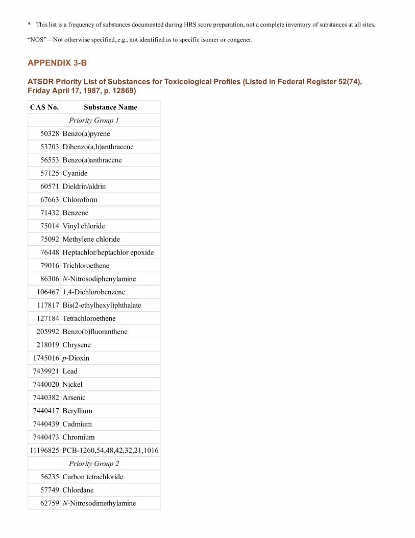


![Supplemental Guidance for Assessing Susceptibility from ...1].pdfrelevant routes of environmental exposure for human cancer risk assessment by EPA, and that these routes of exposure](https://static.documents.pub/doc/80x56/5eda6ddeb3745412b5715342/supplemental-guidance-for-assessing-susceptibility-from-1pdf-relevant-routes.jpg)


