Proceedings of Combustion Institute-Canadian Section Spring Technical Meeting University of Toronto, Ontario May12-14, 2008 HCCI Engine Cyclic Variation Characterization Using Both Chaotic and Statistical Approach Ahmad Ghazimirsaied 1 , Mahdi Shahbakhti, Adrian Audet, Charles Robert Koch Mechanical Engineering Department, University of Alberta, Edmonton, AB T6G 2G8 1 ABSTRACT This paper investigates the cyclic variation of ignition timing in an Homogeneous Charge Compression Ignition (HCCI) engine using a range of experimental data collected from a single-cylinder Ricardo engine. Under certain operating conditions, HCCI engines can exhibit large cyclic variations in ignition timing. Cyclic variability ranging from stochastic to deterministic patterns can be observed. This work applies two methods to study patterns of CA50 (Crank angle of 50% fuel burnt) cyclic variation in an HCCI engine. Nine points ranging from the misfire to knock limit within the HCCI mode are experimentally measured by varying the intake manifold temperature. The return map techniques used in nonlinear dynamics and chaos theory are applied to observe possible deterministic structures inherent in these points. Probability distribution for cyclic combustion timing is the second approach examined. Experimental data of 338 different points over a wide range of operating conditions are examined to find out the conditions where a normal distribution for CA50 is observed. Three common statistical testing methods are used to verify the hypothesis of having a normal distribution for each data point. 2 INTRODUCTION HCCI engines are of great interest to researchers because of their advantages which include very low emission levels and higher efficiency compared to Spark Ignition (SI) and Compression Ignition (CI) engines [1]. On the other hand, these engines have some disadvantages. One of their main drawbacks is the control problem due to the lack of any direct control means to trigger combustion [2, 3]. Methods to extend the HCCI operation range is also a focus for researchers [2]. Cycle-by-cycle experimental observations of important engine parameters have shown an inherent non-random structure inside the SI engine [4]. The presence of deterministic structures suggests that techniques for real-time control to stabilize the unstable operating regions of the engine can be implemented [5]. The transition between spark ignition and HCCI combustion which follows a relatively low-dimensional determin- istic dynamics has been documented in [5]. There the internal EGR (Exhaust Gas Recirculation) is varied by changing the timing and lift of the intake and exhaust valve. In [6], the connection between past and future combustion events are investigated using experimental nonlinear mapping functions. Their results confirm that the deterministic component of lean combustion variations can be approximated by fitting the data to a low-order nonlinear map. Chaotic behavior in a production internal combustion engine has also been documented in [7]. Different patterns of cyclic variation of combustion patterns have been observed in [8] including normal, periodic and cyclic variations with weak/misfired ignitions. This paper is organized as following. In the next section, the experimental setup for collecting the data is briefly described. Then, the engine variation and bifurcation plot are used to describe how the general behavior of CA50 varies as intake manifold temperature changes while other variables are held constant. Return maps from chaotic theory are 1 Corresponding author: [email protected]
Transcript
Proceedings of Combustion Institute-Canadian SectionSpring Technical Meeting
University of Toronto, OntarioMay12-14, 2008
HCCI Engine Cyclic Variation Characterization Using BothChaotic and Statistical Approach
Ahmad Ghazimirsaied1, Mahdi Shahbakhti, Adrian Audet, Charles RobertKoch
Mechanical Engineering Department, University of Alberta, Edmonton, AB T6G 2G8
1 ABSTRACT
This paper investigates the cyclic variation of ignition timing in an Homogeneous Charge Compression Ignition(HCCI) engine using a range of experimental data collected from a single-cylinder Ricardo engine. Under certainoperating conditions, HCCI engines can exhibit large cyclic variations in ignition timing. Cyclic variability rangingfrom stochastic to deterministic patterns can be observed. This work applies two methods to study patterns of CA50(Crank angle of 50% fuel burnt) cyclic variation in an HCCI engine.
Nine points ranging from the misfire to knock limit within the HCCI mode are experimentally measured by varyingthe intake manifold temperature. The return map techniques used in nonlinear dynamics and chaos theory are appliedto observe possible deterministic structures inherent in these points.
Probability distribution for cyclic combustion timing is the second approach examined. Experimental data of 338different points over a wide range of operating conditions are examined to find out the conditions where a normaldistribution for CA50 is observed. Three common statistical testing methods are used to verify the hypothesis ofhaving a normal distribution for each data point.
2 INTRODUCTION
HCCI engines are of great interest to researchers because of their advantages which include very low emissionlevels and higher efficiency compared to Spark Ignition (SI) and Compression Ignition (CI) engines [1]. On the otherhand, these engines have some disadvantages. One of their main drawbacks is the control problem due to the lack ofany direct control means to trigger combustion [2, 3]. Methods to extend the HCCI operation range is also a focusfor researchers [2]. Cycle-by-cycle experimental observations of important engine parameters have shown an inherentnon-random structure inside the SI engine [4]. The presence of deterministic structures suggests that techniques forreal-time control to stabilize the unstable operating regions of the engine can be implemented [5].
The transition between spark ignition and HCCI combustion which follows a relatively low-dimensional determin-istic dynamics has been documented in [5]. There the internal EGR (Exhaust Gas Recirculation) is varied by changingthe timing and lift of the intake and exhaust valve. In [6], the connection between past and future combustion events areinvestigated using experimental nonlinear mapping functions. Their results confirm that the deterministic componentof lean combustion variations can be approximated by fitting the data to a low-order nonlinear map. Chaotic behaviorin a production internal combustion engine has also been documented in [7]. Different patterns of cyclic variation ofcombustion patterns have been observed in [8] including normal, periodic and cyclic variations with weak/misfiredignitions.
This paper is organized as following. In the next section, the experimental setup for collecting the data is brieflydescribed. Then, the engine variation and bifurcation plot are used to describe how the general behavior of CA50 variesas intake manifold temperature changes while other variables are held constant. Return maps from chaotic theory are
used to check the deterministic structure inherent in the data points as intake manifold temperature decreases. Finally,the experimental data is statistically analyzed to examine the normality of probability distributions for a range ofmeasured operating conditions.
3 ENGINE SETUP
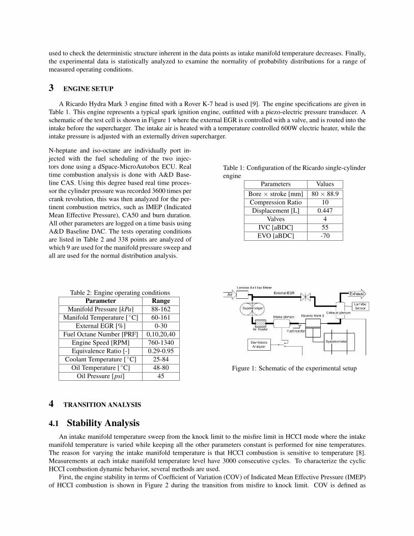
A Ricardo Hydra Mark 3 engine fitted with a Rover K-7 head is used [9]. The engine specifications are given inTable 1. This engine represents a typical spark ignition engine, outfitted with a piezo-electric pressure transducer. Aschematic of the test cell is shown in Figure 1 where the external EGR is controlled with a valve, and is routed into theintake before the supercharger. The intake air is heated with a temperature controlled 600W electric heater, while theintake pressure is adjusted with an externally driven supercharger.
N-heptane and iso-octane are individually port in-jected with the fuel scheduling of the two injec-tors done using a dSpace-MicroAutobox ECU. Realtime combustion analysis is done with A&D Base-line CAS. Using this degree based real time proces-sor the cylinder pressure was recorded 3600 times percrank revolution, this was then analyzed for the per-tinent combustion metrics, such as IMEP (IndicatedMean Effective Pressure), CA50 and burn duration.All other parameters are logged on a time basis usingA&D Baseline DAC. The tests operating conditionsare listed in Table 2 and 338 points are analyzed ofwhich 9 are used for the manifold pressure sweep andall are used for the normal distribution analysis.
Table 1: Configuration of the Ricardo single-cylinderengine
Table 2: Engine operating conditionsParameter Range
Manifold Pressure [kPa] 88-162Manifold Temperature [◦C] 60-161
External EGR [%] 0-30Fuel Octane Number [PRF] 0,10,20,40
Engine Speed [RPM] 760-1340Equivalence Ratio [-] 0.29-0.95
Coolant Temperature [ ◦C] 25-84Oil Temperature [ ◦C] 48-80
Oil Pressure [psi] 45Figure 1: Schematic of the experimental setup
4 TRANSITION ANALYSIS
4.1 Stability AnalysisAn intake manifold temperature sweep from the knock limit to the misfire limit in HCCI mode where the intake
manifold temperature is varied while keeping all the other parameters constant is performed for nine temperatures.The reason for varying the intake manifold temperature is that HCCI combustion is sensitive to temperature [8].Measurements at each intake manifold temperature level have 3000 consecutive cycles. To characterize the cyclicHCCI combustion dynamic behavior, several methods are used.
First, the engine stability in terms of Coefficient of Variation (COV) of Indicated Mean Effective Pressure (IMEP)of HCCI combustion is shown in Figure 2 during the transition from misfire to knock limit. COV is defined as
70 80 90 100 110 120 130 140 1501
2
3
4
5
6
7
8
9
10
Intake Manifold Temperature (oC)
CO
Vim
ep%
MisfireVicinity
KnockVicinity
Figure 2: The coefficient of variation (COV) in theIMEP for intake manifold temperature sweep
70 80 90 100 110 120 130 140 150
0.4
0.6
0.8
1
1.2
1.4
1.6
1.8
Intake Manifold Temperature (oC)
Std
−C
A50
(C
AD
)
MisfireVicinity
KnockVicinity
Figure 3: Variation in STD of CA50 cyclic ensemblefor intake manifold temperature sweep
Standard Deviation (STD) divided by the mean value. The point in the plot with Tman = 80oC, corresponds to the HCCIoperation region near the misfire limit where COV of IMEP is high. As the intake manifold temperature increases,these variations decrease. Near the knock limit region (Tman = 145oC), COV of IMEP reaches to its minimum valuewhich indicates the most stable mode of the combustion.
Since CA50 is a very good indicator of ignition timing in HCCI [10], it is used here as is the cyclic variation ofCA50 during HCCI operation. The Standard Deviation of CA50, which is a good measure of how CA50 variationchanges, is shown in the Figure 3 for varying intake manifold temperature. Increasing the intake manifold temperaturefrom the misfire limit to the knock limit results in CA50 variation decreasing.
A bifurcation diagram is used to reflect the effect of each parameter on the whole time series [11] and is shown inFigure 4 where the variation of the grey scale seen in the plot is indicative of variation in density of CA50 data points.The concentration of data points around their mean point (darker area), increases near the knock limit. In addition,increasing intake manifold temperature advances CA50.
80 90 100 110 120 130 140 150−5
0
5
10
15
Intake Manifold Temperature (oC)
CA
50 (
CA
D a
TD
C)
Figure 4: CA50 bifurcation diagram for intake manifold temperature sweep
4.2 Return Maps
The return maps as a chaotic theory technique is often used to determine the inherent deterministic structure ofthe data [5, 11, 12]. Return maps plot pairs of successive time series values versus each other (here the CA50 valuefor cycle i versus cycle i+1 are plotted in a return map). Using return map plots, each cycle point relates to the nextcycle through the general statistical picture of the whole cycles interrelation [12] and these maps provide a qualitativetool to check the deterministic structure inherent in the data points [13]. The analysis of CA50 for a HCCI sweep
from knock limit to misfire limit during HCCI combustion in terms of the CA50 return maps is illustrated in Figure 5for a range of intake manifold temperatures. The dispersion of these data points over the diagonal line seem to occur
−10 −5 0 5 10−10
−5
0
5
10
CA50(i) (CAD aTDC)
CA
50(i+
1) (
CA
D a
TD
C)
(a) Tman
= 145 (oC)
−10 −5 0 5 10−10
−5
0
5
10
CA50(i) (CAD aTDC)
CA
50(i+
1) (
CA
D a
TD
C))
(b) Tman
= 134 (oC)
−10 −5 0 5 10−10
−5
0
5
10
CA50(i) (CAD aTDC)
CA
50(i+
1) (
CA
D a
TD
C)
(c) Tman
= 128 (oC)
−10 −5 0 5 10−10
−5
0
5
10
CA50(i) (CAD aTDC)
CA
50(i+
1) (
CA
D a
TD
C)
(d) Tman
= 121 (oC)
−10 −5 0 5 10−10
−5
0
5
10
CA50(i) (CAD aTDC)
CA
50(i+
1) (
CA
D a
TD
C)
(e) tman
= 114 (oC)
−10 −5 0 5 10−10
−5
0
5
10
CA50(i) (CAD aTDC)
CA
50(i+
1) (
CA
D a
TD
C)
(f) Tman
= 108 (oC)
−10 −5 0 5 10−10
−5
0
5
10
CA50(i) (CAD aTDC)
CA
50(i+
1) (
CA
D a
TD
C))
(g) Tman
= 99 (oC)
0 5 10 15 200
5
10
15
20
(h) Tman
= 91 (oC)
CA50(i) (CAD aTDC)
CA
50(i+
1) (
CA
D a
TD
C)
0 5 10 15 200
5
10
15
20
CA50(i) (CAD aTDC)
CA
50(i+
1) (
CA
D a
TD
C))
(i) Tman
= 80 (oC)
Figure 5: CA50 Return maps for HCCI combustion illustrating the transition from (a) knock limit to (i) misfire limitreducing the intake manifold temperature
because of nonstationary or transient dynamics of the engine near misfire limit, where oscillations between early andlate CA50 occur frequently. Return maps result for CA50 near the knock limit show an unstructured cluster of circulardata gathered around a fixed point which indicates the HCCI combustion is getting more stable in the vicinity of theknock limit. These data points start to scatter over the diagonal line as they move towards the misfire limit and fixedpoints becomes destabilized leading to more structured data points. The structured patterns seen in the data can beattributed to the deterministic coupling between consecutive cycles. Overall, the return maps exhibit more asymmetryas they approach to the misfire limit.
5 NORMAL DISTRIBUTION ANALYSIS
The second method for analyzing the cycle to cycle combustion timing is using statistical methods. The populationof consecutive ignitions at a constant operating point can be used to form a probability distribution for cycle to cyclecombustion timing. Normal distribution is the most common probability distribution used to characterize experimentaldata [14]. Experimental data at 338 different points including the 9 points analyzed previously are analyzed to deter-mine which conditions have a normal distribution for CA50. Two common testing methods for normal distributionsare used. The first method is the Lilliefors test that evaluates the input data and returns the result of the hypothesistest for the goodness of fit to the normal distribution [15]. The second method is the Kolmogorov-Smirnov test thatcompares the values in the data with a standard normal distribution and checks the hypothesis that the data has astandard normal distribution [16, 17]. These two methods are applied on the CA50 data sets from 338 points. Pointsthat successfully pass these two tests are then visually evaluated with normal probability plot. The normal probabilityplot is a graphical tool to assess whether or not a data set follows a pattern of a normal distribution [14]. Data from theexperimental points are plotted against a theoretical normal distribution and if data is normally distributed, it forms
an approximate straight line. The level of departures from normality is judged by how far the points vary from thestraight line. Figure 6 shows a normal probability plot for a sample experimental point that exhibits a normal distribu-
−1.5 −1 −0.5 0 0.5 1 1.5 20.00010.00050.001
0.0050.01
0.050.1
0.25
0.5
0.75
0.90.95
0.990.9950.9990.9995
0.9999
CA50 [CAD aTDC]
Nor
mal
Pro
babi
lity
Figure 6: Sample normal probability plot for the test point (h) in Figure 5.
tion. CA50 data sets for all experimental points were processed using the procedure mentioned above and 19 pointsout of 338 points are judged to have a normal distribution. The range of ignition timing parameters for cases withnormal distribution are compared with those of the whole data set in Table 3.
Table 3: Comparing the range of ignition timing parameters for cases with normal distributions with those from thewhole 338 HCCI experiments
Table 3 shows that normal distribution of CA50 is more likely to occur in HCCI ignitions occurring for a windowimmediately after TDC (0.8 ≤ SOC ≤7.7 CAD aTDC). In those conditions, cyclic variations of CA50 is typicallylow (0.4 ≤ ST DCA50 ≤1.4 CAD) and the burn duration is short (2.5 ≤ BD ≤ 4.3 CAD). A large deviation from thestraight line is observed in normal probability plots of the operating points which have mean CA50 occurring after 15CAD aTDC. Furthermore, all the 19 test points are for fully warmed up conditions and none of the points which havelow coolant temperature show a normal distribution for CA50. No direct preference for normal distribution was seenin operating conditions in terms of octane number, engine speed, equivalence ratio and intake conditions. However, acombination of these conditions determine the location of SOC.
6 CONCLUSIONS
Experimental characterization of cyclic variation of HCCI combustion using both chaotic and statistical methodshas been performed.
Using bifurcation diagrams and return maps more structure is observed as the engine operating condition ischanged from the knock limit to the misfire limit by using 9 different intake manifold temperatures. This struc-ture is indicative of a coupling between successive CA50 (engine cycle timing) which has the expected sequence oflate and early combustion near the misfire limit.
A wide range of engine operating conditions (338 points) are analyzed using normal distribution variation statis-tical tests. As expected, stable HCCI combustion with combustion timing near TDC is more likely to have normaldistributions since the combustion timing of successive cycles is independent.
7 ACKNOWLEDGMENT
The authors gratefully acknowledge AUTO21 Network of Centres of Excellence, the Canadian Foundation forInnovation (CFI) and the Natural Sciences and Engineering Research Council of Canada (NSERC) for supporting thiswork.
and future engine applications. SAE Paper No. 1999-01-3682., 108, 1999.
[2] T. Urushihara, K. Yamaguchi, K. Yoshizawa, and T. Itoh. A Study of a Gasoline-fueled Compression IgnitionEngine Expansion of HCCI Operation Range Using SI Combustion as a Trigger of Compression Ignition. SAEPaper No. 2005-01-0180., 2005.
[3] M. Weinrotter, E. Wintner, K. Iskra, and T. Neger. Optical Diagnostics of Laser-Induced and Spark Plug-AssistedHCCI Combustion. SAE Paper No. 2005-01-0129., 2005.
[4] R.M. Wagner, J.A. Drallmeier, and C.S. Daw. Prior-cycle effects in lean spark ignition combustion - fuel/aircharge considerations. SAE Special Publications, pages 69–79, 1998.
[5] R.M. Wagner, K.D. Edwards, C.S. Daw, J.B. J.r. Green, and B.G. Bunting. On the nature of cyclic dispersion inspark assisted hcci combustion. SAE Paper No. 2006-01-0418., 2006.
[6] R.M. Wagner, C.S. Daw, and J.B. J.r. Green. Low-order map approximations of lean cyclic dispersion in pre-mixed spark ignition engines. SAE Paper No. 2001-01-3559., 2001.
[7] L. Chew, R.L. Hoekstra, and J.F. Nayfeh. Chaos analysis on in-cylinder pressure measurements. SAE Paper No.942486., 1994.
[8] M. Shahbakhti, R. Lupul, A. Audet, and C. R. Koch. Experimental study of hcci cyclic variations for low-octaneprf fuel blends. Proceeding of Combustion Institute/Canadian Section (CI/CS) Spring Technical Conference,2007.
[9] R. Lupul. Steady State and Transient Characterization of a HCCI Engine with Varying Octane Fuel. Master’sthesis, University of Alberta, 2008.
[10] J. Bengtsson. Closed-Loop Control of HCCI Engine Dynamics,. PhD thesis, Lund Institute of Technology,, 2004.
[11] R.M. Wagner, J.A. Drallmeier, and C.S. Daw. Origins of cyclic dispersion patterns in spark ignition engines.Proceedings of the 1998 Technical Meeting of the Central States Section of the Combustion Institute, pages213–218., 1998.
[12] J.B. J.r. Green, C.S. Daw, J.S. Armfield, and C.E.A. Finney. Time irreversibility and comparison of cyclic-variability models. SAE Paper No. 1999-01-0221., 1998.
[13] J.B. J.r. Green, C.S. Daw, J.S. Armfield, C.E.A. Finney, and P. Durbetaki. Time irreversibility of cycle-by-cycleengine combustion variations. Proceedings of the 1998 Technical Meeting of the Central States Section of theCombustion Institute, 1998.
[14] NIST/SEMATECH e-Handbook of Statistical Methods http://www.itl.nist.gov/div898/handbook/, Jan. 20, 2008.
[15] H. Lilliefors. On the Kolmogorov-Smirnov Test for Normality with Mean and Variance Unknown. Journal ofthe American Statistical Association, 62:399–402, 1967.
[16] A. N. Kolmogorov. On the Empirical Determination of a Distribution Function. (Italian) Giornale dell’InstitutoItaliano degli Attuari, 4:83–91, 1933.
[17] N. V. Smirnov. On the Estimation of the Discrepancy Between Empirical Curves of Distribution for Two Inde-pendent Samples. (Russian) Bulletin of Moscow University, 2:3–16, 1939.


![HCCI - Update of Progress 2005 - US Department of Energy · HCCI – Update of Progress 2005 HCCI HCCI ... M EP [b a r] B S F C [g/k W-hr] ... Typically used in 2-Stroke Engines at](https://static.documents.pub/doc/80x56/5ac4ebc77f8b9a220b8d1053/hcci-update-of-progress-2005-us-department-of-energy-update-of-progress.jpg)


