Health plan type variations in spells of health care...

1

Health plan type variations in spells of health care treatment

Randall P. Ellis and Wenjia Zhu

Boston University

August 21, 2015

Acknowledgements. We are grateful to Arlene Ash, Francesco Decarolis, Tim Layton, Tom McGuire, Erik Schokkaert, Frank Sloan, and participants at the American Society of Health Economists and the Risk Adjustment Network for useful comments and insights, although the authors bear full responsibility for any errors or omissions. This research was partially supported by Verisk Health through a grant to Boston University.

Keywords: health care spending, treatment spells, risk adjustment, exclusive provider organizations, consumer driven health plans

JEL codes: I11, G22, I13

Abstract:

This paper analyzes 30-day “treatment spells” - fixed length periods that commence with a service after a gap in provider contact - to examine how health care utilization and spending of insured employees at large firms are influenced by health plan types. We focus on differences between preferred provider organizations (PPOs) and two recent innovations: plans that feature a narrow panel of providers, and plans that allow free choice of providers but increase demand-side cost sharing: consumer-driven/high-deductible health plans. Health plan effect estimates change dramatically after controlling for endogenous plan type choice, and individual fixed effects. With these controls, narrow panel plans reduce the probability of new treatment spells relative to PPOs by 34 percent with little effect on chronic, repeat visit spells. Visit reductions are more concentrated in less severe conditions in narrow network plans, hence diagnostic coding on the remaining patients increases. We find no evidence that either narrow panel or higher cost sharing plans pay lower prices per procedure or have less intensive treatment given initiation of treatment. With controls, consumer-driven/high-deductible health plans are associated with higher total spending on procedures than PPO plans.

2

Section1:IntroductionUnderstanding how to control health care costs is perhaps the central challenge facing all health care systems, and hence explaining how health care costs are influenced by health plan design features is of particular policy interest. In the US, both public and private insurers are experimenting with diverse new health plan designs, and the new Health Insurance Marketplace established by the Affordable Care Act (ACA) promotes plan design variation on both demand-side cost sharing and supply-side provider networks in the individual and small group markets. Of particular interest are two new health plan types that are growing in market share: (1) plans with narrow panels of providers that rely on careful supply side selection of providers by health plans, and (2) plans with little or no restrictions on provider choice that rely on high demand-side cost sharing to encourage consumers to shop around for low cost providers. The broad question this paper addresses is which of these plan type innovations is more effective at reducing health care expenditures in the well-insured, large employer private insurance market.

Comparisons of US health care spending with Europe and Canada find that US expenditures are high because prices per service are high, and because the US health care system uses more services for a given health condition (i.e., higher “treatment intensity”). (Anderson et al. 2003; Lorenzoni, Belloni, and Sassi 2014). Recent studies also find that price variation and treatment intensity variation contribute significantly to the large geographic variation in costs within the US (Chernew et al. 2010; Romley et al. 2015). A third contributing factor is that US health care providers, incentivized by generous fees, frequent patient contacts, and abundant test results, identify and treat more health conditions than in other countries, which shows up as increased diagnostic “coding intensity” on insurance claims (Wennberg et al. 2014). Routine breast and colon cancer exams, magnetic resonance imaging (MRI) and increased laboratory testing are all examples of potentially greater disease identification in the US.1

A popular view in the US is that competition should be used to control costs. But it remains unclear whether demand side incentives such as cost sharing that encourage consumers to be cost sensitive are more or less effective at reducing costs than supply-side incentives such as selective provider contracting that relies on competing health plans to find low price, low treatment intensity, or less aggressive providers. Also important is how demand-side cost sharing and supply-side incentives reduce spending.

The general finding in the literature on the demand side is that cost sharing reduces health care utilization with heterogeneous effects depending on types of services (Duarte 2012), stages of treatment (Manning et al. 1987) and one’s location in the expenditure distribution (Kowalski 2015). If consumers are not well informed about their health, demand-side cost sharing may motivate consumers to skip important services (Galbraith et al. 2012). A different concern is that well-informed consumers seeking high-cost services may well reach their deductibles and stop-

1 Hospital’s strategic diagnostic coding, often called “Diagnosis Related Group (DRG) creep”, is one example of what we term increased “coding intensity”, in which hospitals increase the number of coded diagnoses to make their patients look sicker in order to increase revenue subsequent to the introduction of hospital DRGs in 1983 by the US Medicare program, and subsequently by most payers (Steinwald and Dummit 1989). Such record-keeping practices may affect all types of providers and services, not just hospitals. Note that the coding intensity of a plan type will also increase if consumers with low severity problems are more likely to reduce their visits due to demand or supply incentives than consumers with more severe problems.

3

loss amounts so that demand-side incentives have little influence on the health care utilization of these people (Kowalski 2015). On balance, it is the entire cost share structure, not just a single price that matters in consumers’ health care decisions (Ellis 1986; Einav, Finkelstein, and Schrimpf 2015; Aron-Dine et al. 2015). The effects of supply-side incentives, in particular narrow provider networks, are less well studied than demand-side incentives. While Gruber and McKnight (2014)’s study of narrow provider networks in Massachusetts suggests that cost savings can be significant using a limited network, Peters and Holahan (2014)’s study of the ACA Health Insurance Marketplace in six cities reports that narrower provider networks, usually but do not always lower premiums. Few previous studies attempt to explain the variations in health spending in a uniform framework where both consumer and provider incentives are considered, with the notable exceptions being Altman, Cutler, and Zeckhauser (2003) and Cutler et al. (2015).2 Our paper extends the literature by studying plan type effects on both the consumer and provider incentives in a large, multiple-employer, multiple-insurer panel dataset where diverse supply- and demand-side incentives are present.

Ultimately, we are interested in whether and how savings on health care spending can be achieved by plan designs through their impacts on consumer and provider incentives. Our paper centers around this issue by answering three types of questions. First, we evaluate the overall effect of different health plan types on consumers’ incentives to seek care. We then turn to studying what types of care are most affected: are consumers deterred from making initial visits, follow-up visits, or repeated visits over three or more months? The final area we explore is whether and how savings are achieved conditional on consumers deciding to seek care. Are savings achieved via lower prices, lower treatment intensity, or a lower provider effort at identifying diseases to treat (or code) for a given symptom? Section 3 lays out a conceptual framework underlying our approach.

Three innovations distinguish our conceptual framework from the existing literature. First, we focus on a unit of analysis called treatment spells as an alternative to episode and calendar interval analyses. As discussed in Section 2, treatment spells are more attractive for analyzing health care treatment decisions than annual or monthly periods for clinical and statistical reasons and simpler than episodes. Second, we separately estimate models of subsets of treatment spells, based on whether each spell is a new visit spell (following 30 days with no treatment), a continuation visit spell (following a new spell) or what we call a chronic visit spell (which follows a continuation or previous chronic visit spell), enabling us to distinguish whether plan types are disproportionately affecting new, continuation or chronic visit spells of treatment. Third, we decompose spending in a spell month into five multiplicative components – the probability of a visit, the level of prices, treatment intensity, an original measure we call coding intensity, and a term capturing patient severity of illness at the time of seeking care. This payment decomposition, discussed in more detail in Section 3, enables us to better identify how cost savings are achieved by different health plan types.

We understand that our analysis of only three spell types is highly simplified (although many other studies focus only on total annual spending). A natural extension of our spell approach would be to classify spells more finely, such as by the presence or first onset of a specific 2 Cutler et al. (2015) use survey results to decompose variations in health care spending according to demand-side and supply-side incentives.

4

disease, the occurrence of certain procedures or events (such as knee transplants, cancer biopsy, or emergency department visits), or to assign spells to a specific provider. We leave these extensions to future papers, focusing on a broad overview here.

Our estimation methods accommodate a number of econometric challenges. All of our models carefully incorporate risk adjustment measures that use diagnoses, age and gender to reflect the consumers’ information about their health at each stage of the decision making processes – plan choice, the decision to seek care, prices, treatment intensity and coding intensity. Individual, county, time, and employer fixed effects further control for demand- and supply-side variation so that plan type effects are identified solely by consumers’ movement between health plan types within our sample periods. Two stage least squares (2SLS) estimates are used to control for endogeneity of health plan type choices: plan type dummies are instrumented by fitted probabilities of choosing each plan type that incorporate household variables on employee age and gender, family size, the presence of a baby or spouse, health risk, and the list of plan types offered by the employer in that year. We use two methods to correct standard errors for clustered errors. Our primary approach is to calculate cluster-robust corrected standard error at the level of employer, year, and family versus individual coverage types to avoid overstating model precision. Alternatively, we use bootstrapping methods to re-estimate our full models on 100 random samples of our data and generate confidence intervals from the empirical distribution of the estimates. Details about econometric issues are provided in Section 4.

To give a preview, our results in Section 6 suggest that narrow panel health plans do better at reducing costs and utilization than high cost sharing plans, relative to preferred provider organizations (PPOs), which are the most widespread health plan type in the US.3 Although narrow panel plans and high cost sharing plans appear to save money relative to PPOs when comparing sample means or using simple OLS models, most of these savings disappear once we control for endogenous plan type choice, individual fixed effects and patient severity of illness. Narrow provider panel plans significantly reduce the probability of new treatment, with little effect on repeat visits for chronic conditions. Decomposition of total spending suggests that none of the plan types is successful at reducing prices relative to PPOs, with some evidence that prices are higher in high-deductible plans. Providers’ treatment intensity explains little of the variation in health spending across different plan types. We find more statistically significant differences across plan types in our new measure of coding intensity conditional on a disease than in prices or treatment intensity. In particular, narrow panel plans code patients more aggressively than high cost sharing plans, likely a result of disproportional reduction in less severe spells of treatment in narrow network plans than in high-deductible plans. Overall, high cost sharing plans are found to have higher total spending on procedures once we control for endogenous plan type choice, individual fixed effects and patient severity of illness. We return to discuss these findings more after presenting our methods, data and results.

3 For readers unfamiliar with the organization forms of health plans in the US, Section 3.1 provides a brief introduction of the institutional background and evolution of health plan types in the US.

5

Section2:Spellsoftreatmentapproach

Section2.1:RationaleWhile a year is a convenient unit of observation for studying how broad patient characteristics affect spending and utilization, a year is too coarse for examining most consumer and provider decisions: a patient will often see many providers and have multiple spells of treatment in a given year. Keeler and colleagues at the RAND Corporation were the first to provide a careful and comprehensive study of health care spending and utilization patterns using an episode approach (Keeler et al. 1982; Keeler et al. 1986; Keeler and Rolph 1988). Episodes of treatment begin with a clinical assessment of a new condition, continue while that condition is being treated, and end once no further visits are observed for a period of time. While attractive conceptually, remarkably few published academic studies have used episodes to study outpatient treatment patterns.4 This mostly reflects practical issues of distinguishing multiple, overlapping episodes, deciding when information becomes known and when continuation decisions are made, dealing with incomplete episodes at the start and end of the sample period, and incorporating chronic illnesses that may persist indefinitely.

A second and related approach is to use monthly spending and utilization measures. Ellis (1986) and Manning et al. (1987) were early users of this approach, with more recent examples being Eichner (1998), Einav et al. (2013) and Einav, Finkelstein, and Schrimpf (2015). In order to model the effect of deductibles and stop-losses, which change consumer out of pocket costs during the calendar year, all of these studies use a month as the unit of observation, and use variations in health care cost sharing within a year to study demand effects. Similar to episodes, monthly models are challenged in capturing multiple conditions and dealing with beginning- and end-of-sample truncations. A further weakness of fixed calendar months is that they artificially split up diseases and associated treatment patterns when treatment spans multiple months.

The treatment spell approach used here lies intermediate between episodes and monthly analysis, and has its origins in the early work of Keeler, Manning, and Wells (1988) in modeling demand patterns of mental health treatment. Treatment spells also underlie the Medicare payment system for paying for home health (Fed. Reg. 2013) and many studies of care following an inpatient admission. Similarly to episodes, a “new visit” spell starts with an office visit or the beginning of a service after a period of time with no visit/treatment, and last for a fixed time interval of 30 (or 31) days with the last day of this period marked as the ending of the treatment spell.5 This is different from the episode approach where typically the completion of a treatment marks the ending of an episode. In our framework, following each treatment spell is either a “no visit” spell or another treatment spell. Since treatment spells need not start on the first day of the calendar month, then neither do “no visit” spells: If no visit/treatment is observed within a 30 day period, then we have “no visit” spell(s) until the presence of a new visit that marks the beginning of a

4 For discussion of this issue, see MaCurdy et al. (2008) and Rosen et al. (2012). Both papers apply two most commercially available episode groupers, Episode Treatment Groups (ETGs) and Medical Episode Groups (MEGs), to form episodes from claims and assign costs to episode. MaCurdy et al. (2008) focus on using Medicare claims as inputs, while Rosen et al. (2012) uses commercial claims data. Both discuss challenges associated with matching and comparing results from different groupers. 5 We alternate between assigning each treatment spell month 30 or 31 days, and assigning spell month twelve 30 or 31 days according to whether it is a leap year.

6

new treatment spell. The treatment spell approach facilitates modeling decisions of the initialization and continuation of health care treatment over fixed 30-day periods that is missed by using fixed monthly periods, while also allowing multiple decision points which are often missed when creating episodes.6

Unlike Keeler et al. (1988) and most episode groupers, we do not attempt to uniquely assign utilization and spending variables to distinct illnesses, but instead view treatment as generally related to many conditions. For example, we do not classify a treatment spell as a diabetic, hypertensive or mental health spell, but instead use a risk adjustment framework to capture any number of conditions within the spell.7 For this paper, we do, however, distinguish between three categories of treatment spells (Figure 1). Following a period of at least 30 days with no visits, we have “new visit” spells, which may or may not be followed by a “continuation visit” spell. If a “continuation visit” spell is followed by a third (or more) spell of treatment, we classify such spells as “chronic visit” spells. Fitting around our fixed length treatment spells are “no visit” spells of variable length, which are simple to model since by construction there are no visits or spending in them. Figure 1 illustrates how office visits (denoted as “V”), hospital stays (denoted as “H”), and emergency department visits (denoted as “ER”) by one person can be grouped into new, continuation, and chronic spells of treatment, as well as into “no visit” spells that lie in between them.

Section2.2:Whyspellsarebetter?We employ a treatment spell approach for both clinical and statistical reasons. The main argument in favor of treatment spells over months and quarters is clinical validity. On the one hand, fixed monthly calendar intervals inherently split many spells of treatment across multiple periods, and do not usually correspond to clinical decision making units. For example, follow-up visits at 7, 14 and 28 days are common, and will all tend to belong to a single treatment spell month, but they do not necessarily fit into a single calendar month. On the other hand, longer periods such as a calendar year or quarter, while easier to model than months and less likely to split up treatment decisions, aggregate new information and diverse decisions into a single unit.8

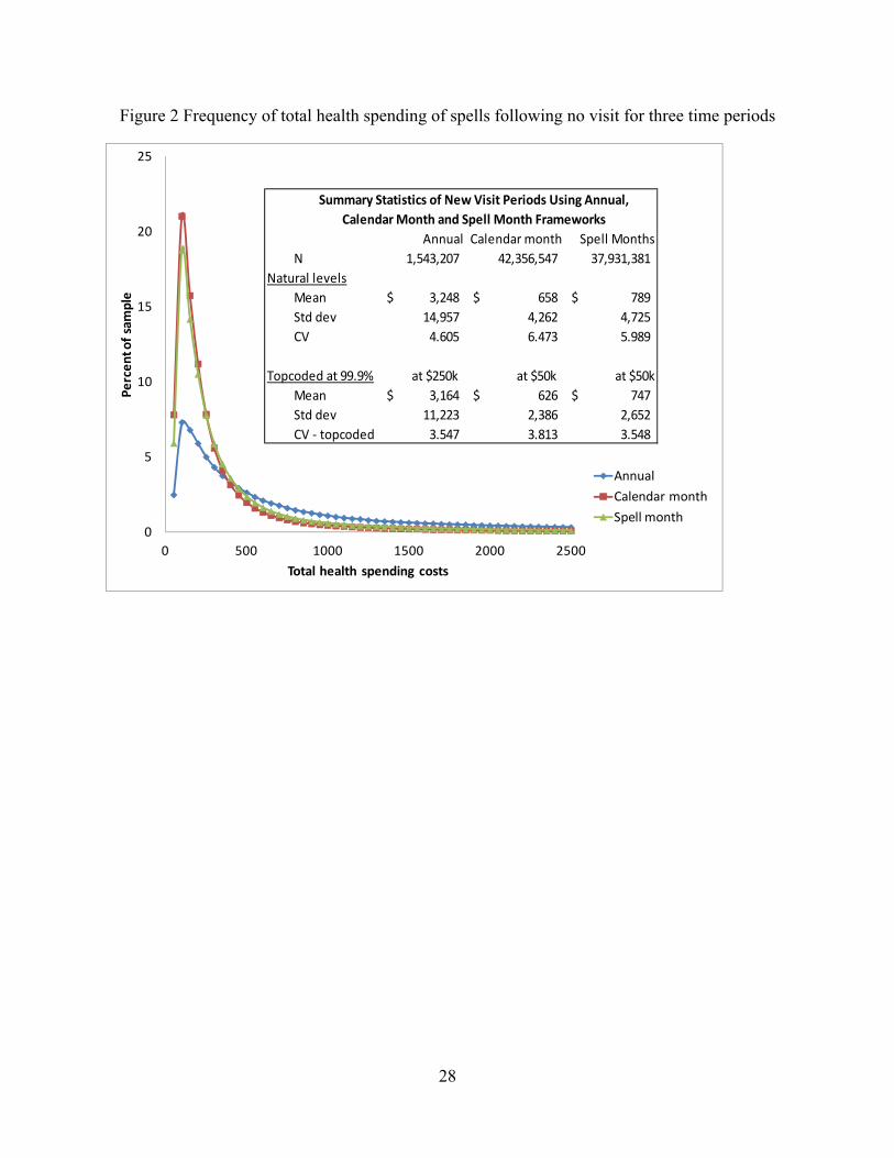
The second argument in favor of treatment spells is statistical. To explore this, we plot the distributions of health spending under three time periods (calendar year, calendar month, spell

6 Consider a hypothetical patient who receives a colonoscopy that identifies a polyp in the colon in mid-November that is found to be malignant and ultimately undergoes 120 days of radiation and chemotherapy treatment. Using an annual observation, this episode of treatment would be divided up into two years, both of which will be lower cost than if the cancer had been identified in July. Using a fixed calendar month unit of observation, this patient would have half a month of initial cancer treatment and three and a half further months of high costs and utilization. Using an episode approach, all of the four months of treatment decisions would be collapsed into a single episode observation, as if there was only one treatment decision made by patients and doctors. Finally, in a spell of treatment approach, one would look at resource use in the first 30 days of new treatment, the second, third and fourth continuation months of treatment. If one believes that new information is obtained during an episode or year and that new decisions are made based on that information, then spells of treatment may be more useful than fixed time periods or episodes. 7 A treatment spell approach can be easily extended to keep track of treatment patterns associated with specific conditions or illnesses, the use of specific services or drugs, or other triggering events. We use the onset of treatment after 30 days with no visits as our triggering event. 8 Although we do not explore this use here, shorter treatment spells are also easier to assign to a single primary care provider than longer periods of time, whether a year or a long episode.

7

month) in Figure 2, with summary statistics shown in the box. Each point in the figure is the percentage of total observations that falls into each of the fixed-dollar windows ($50 in our experiment) along the distribution. We drop observations with negative payments and focus on “new visit” spells, namely spells following a period of at least 30 days with no visits. We report both the natural and the top-coded spending at $250,000 annually and $50,000 monthly, both values of which correspond to the 99.99th percentiles of spending. Figure 2 shows that spending is less dispersed at the treatment spell than at the calendar month level, and the variation in spending at the spell month level is closer to that under the annual framework when spending is topcoded (the last row in the box).

Section3:Conceptualframework

Section3.1:ChoiceofhealthplansEach year an employer chooses a set of health plans offered to employees. Employees in turn choose from among the available health plans, with choices reflecting plan characteristics, employee demographics, employer, and household health status. We assume that choice of health plans is determined at the beginning of each year, and is fixed throughout the year.9

The analysis of plan choice and plan types presented here is best understood in the context of the evolution of health plan types in the US. Fifty years ago, almost all large firms offered a single health plan, which in today’s terminology would be comprehensive plans (abbreviated here as COMPs), with modest cost sharing, no restrictions on provider choice, and little effort to manage care. The first major plan type innovations were health maintenance organizations (HMOs) which contracted with a limited set of providers, negotiated reduced fees, and typically “managed care” in the sense that providers often would have the plan or its agents oversee the services provided. In the 1990s, there was a backlash against HMOs form of managed care, despite the evidence that HMOs are successful at reducing costs (Dugan 2014; Newhouse and McGuire 2014).

The next popular plan type to emerge was preferred provider organizations (PPOs) which negotiated reduced fees and typically included a somewhat limited set of providers but with less tight management. PPOs range widely in their cost sharing features, and are now the most popular plan type among large employers. In order to motivate enrollees to use higher quality or lower price providers, point of service plans (POS) emerged in the 1990s that introduced the concept of tiers of providers, with some “in network” providers given lower consumer cost shares than out of network providers, with the latter still eligible for some coverage.10 These four plan types - COMP, HMO, PPO, and POS plans - represented more than 99 percent of all health

9 Among the 7 percent of our employees who switch plan types each year in our continuously-eligible sample, over 90 percent of the switches happened on January 1. Switches can occur because of births, marriage, divorces, sabbaticals, moving, and need not mean that the plan year differed from the calendar year. We did not find any plans where the majority of switches occurred at a month other than January 1. 10 Some HMOs, PPOs and POS plans pay some providers using capitation (monthly payments) rather than fee for service reimbursement. These types of payments also dominate spells of treatment in a “Point of Service with Capitation” plan type. Altogether spell months involving capitation payments amount to about 3 percent of all the spells in our initial sample. As described in our Appendix B.2, we have omitted all such spells from our analysis since prices and costs of individual services cannot be reliably measured.

8

plan enrollments in large employers in 2004 when other, newer plan types began to emerge (Ash and Ellis 2012, Table A3).

Since 2004, two new plan types have become popular. One plan type is exclusive provider organizations (EPOs) that greatly restrict consumer choice of providers while deemphasizing demand side cost sharing. It is subjective where the boundary is between EPOs and HMOs: we rely on our data vendor’s assessment of this distinction (Truven Health Analytics). Some EPOs are as narrow as the providers employed at a single hospital or medical school, while others are statewide networks of carefully chosen providers. The second new plan type is consumer-driven/high-deductible health plans (CDHDs) that promote wider consumer choice but raise consumer cost sharing.11 As with EPOs, there are subjective boundary issues between PPOs and CDHD plans, but we rely on the classification system of the data vendor to identify plan types in our analysis (see more discussion of our data source in Section 4.1 and Appendix B).

Our study focuses on spending and utilization differences among six plan types. These include four traditional plan types – COMP, PPOs, HMOs and POS – which still represent the majority of the all health plan enrollment in the US. We use the PPO plan as the comparison group since it has the largest number of enrollees and is the most commonly offered plan type. The two new plan types of great interest are CDHDs which we classify as the increased demand-side cost sharing plan, and EPOs that rely primarily on supply side choices made by health plans. Table 1 provides details about each plan type, sorting plan types according to their extent of consumer choice of providers. The last column of this table shows the average cost sharing of different plan types in the analysis sample (see more details about sample creation in Section 5.1 and Appendix B). We find that the empirical cost sharing is consistent with the general perception of these plan types. We also find that higher cost sharing plan types are in general less restrictive on choice of provider panels, which highlights the tradeoff that dominates most US health plans. Figure 3 summarizes enrollment trends in the six plan types being studied here.

Section3.2:DecompositionofhealthcarespendingWe decompose total spending on each monthly spell of treatment into five components in order to understand the underlying factors that contribute to plan type variation in spending. Using total spending during a spell month as our measure (which includes both consumer paid and plan paid spending), we use the following equation in which the variables i, j, s, and t index patient, provider, service, and spell month, respectively.

11 As McKellar et al. (2012), Bonafede et al. (2013) and Arondekar et al. (2015) have done on the same dataset, we choose to combine consumer-driven health plans (CDHP) and high-deductible health plans (HDHP). The two plan types share similar properties: both generally do not restrict choices to a specific panel of providers, involve high deductibles and significant cost sharing, and set aside money earmarked to the consumer that can be used to pay the consumer’s cost share using pre-tax dollars. Where they differ is that HDHP plans use a flexible spending account that cannot be rolled over from one year to the next, often called “use it or lose it” account, while CDHPs use a health care savings account that can be saved across multiple years to pay for future health care costs.

9

,

Pr 0 | 0

Pr 0∑

∑ .

∑ .

.

.

.. ..

(1)

Equation (1) is an identity and each component in brackets can be calculated empirically. The first term in brackets is the visit decision, which is the probability of starting or continuing a spell of treatment in a given month, and thereby incurring positive spending. The second term is a conventional price index with weights being the spell’s actual quantities, using the provider’s actual prices in the numerator and national average prices in the denominator. Both provider actual prices and national average prices are adjusted to account for inflation and geographic variation in provider costs. The third term is a measure of treatment intensity. The numerator uses national average prices of each service to weight actual quantities provided during the spell. The denominator . , is a measure of predicted spending given the diseases concurrently assigned by the patient i’s own provider j for that month of treatment t. Overall this third expression reflects the amount of services provided to patient i during the spell given condition diagnosed by provider j in that spell. Intuitively, this term is the quantity of services, as measured using the national procedure price average, relative to how sick the patients are as measured by coding by providers for that spell of treatment, which we discuss further below.

The fourth term in brackets is our measure of coding intensity. It is the ratio of two risk adjustment predictions. The numerator of this term, matching the preceding denominator, is the expected cost given the provider’s own concurrently assigned diagnoses during the current spell month of treatment. The denominator, as well as the final term in brackets, .. , ,is a different measure of expected spending, capturing the consumer’s expected spending (or patient severity) at the time of making the decision to seek treatment. At a minimum, it should include the diseases known to the consumer from the prior twelve months, but the consumer may also know something about the nature of their current spell (e.g., an injured shoulder, sore throat, feeling of sadness). We interpret the fourth term in brackets as a measure of coding severity in that the broad body system used in the final severity adjustment (skin problem, heart problem, mental health disorder etc.) is something mostly observable by the patient at the time that a visit is initialized, while the detailed diagnoses of this condition is something that requires a clinician.12 We posit that this measure partly captures how much effort providers put into identifying and writing down more detailed, specific diagnoses, a decision that is potentially influenced by the health plan type. The fifth term in brackets is a conventional risk score measure of patient severity, using lagged information and coarse information about conditions diagnosed during the current spell month.

All five components in our decomposition (1) are potentially subject to demand- and supply-side incentives induced by plan design features. The final term – severity – has been included in the 12 The detailed diagnoses of conditions are also potentially influenced by the patient, as patients sometimes know more about their health than providers. In those cases, patients may help providers to find more problems depending on how conversations go between the two parties (e.g. patients self-report previous diagnoses that facilitate future diagnoses by providers). We provide further justifications for our measure of coding intensity in Section 3.5.

10

decomposition to form an identity, so part of its association with either consumer or provider incentives will be captured in the coding intensity measure. If severity varies by plan type, it is a signal of adverse selection. Below we discuss further the hypothesized health plan type effects on probability of visits (Section 3.4), prices (Section 3.6), treatment and coding intensities (Section 3.6).

Section3.3:Subsetsoftreatmentspellsexamined We use our treatment spell modeling approach to examine the overall probability of a visit and then distinguish between different spell types. Using N, V and C to denote no visit, new visit, and continuation spells, we model the probability of a visit conditional on the previous spell month information, namely the three probabilities Pr(V|N-1), Pr(C|V-1), and Pr(C|C-1), where the negative one denotes the treatment spell of the consumer in the prior spell month. (Appendix Table A-1 describes the spell transition matrix underling this approach.)

Section3.4:HealthplantypesandincentivestoseekcareIt is theoretically ambiguous whether demand-side cost sharing that encourages consumers to be cost sensitive is more or less effective at reducing care seeking than supply-side incentives such as selective provider contracting. On the one hand, higher cost sharing reduces a consumer’s incentive to initiate treatment while having little influence on the incentive to supply care provided that payments to providers remain stable. Since new treatment spells are mostly initiated by consumers, while continuation visits are more likely to be initiated by provider recommendations, we would expect demand-side cost sharing to have a greater impact on new than continuation spells. On the other hand, supply-side incentives may potentially have a greater impact than demand-side incentives on consumers’ care seeking behaviors. It is possible that narrow provider panels makes new care seeking less attractive: consumers in supply-side constrained plans, such as HMOs and EPOs, may internalize the less aggressive disease identification and treatment, and may be less inclined to seek care than consumers in plans less constrained on provider networks. It is also possible that a narrow network creates an expectation of higher effort by health plans to choose high quality, low cost providers to manage care, generating a greater incentive for consumers to seek care.

Section3.5:CodingIntensityCoding intensity variation and strategic diagnostic coding have recently received considerable attention, perhaps because of the increased use of risk adjustment in the ACA. Wennberg and colleagues (2013, 2014) have challenged the Medicare risk adjustment formula by arguing that the Medicare formula unduly reflects variation in coding intensity as well as variation in severity (for a contrary view, see Newhouse et al. 2013). Geruso and Layton (2014) find evidence of statistically significant coding intensity increases on the order of 7 percent in response to risk-adjusted payments in private Medicare Advantage plans. Further evidence of strategic coding is provided by Kronick and Welch (2014). To explore this issue, we develop a novel method for calculating coding intensity and use it to examine whether coding intensity appears to be responsive to plan types within our sample.

The rationale for our coding intensity measure is as follows. For most health conditions, the consumer will know what broad body system is ill even before seeing a doctor, and hence a relatively crude diagnosis classification system captures reasonably well the consumer’s information at the time that care is sought. In contrast, only a physician can distinguish among the thousands of more specific diagnoses, particularly those associated with the highest cost and

11

greatest severity. We therefore decompose the conventional risk score measure of health status into two components. The first component predicts health care spending using only broad categories of health conditions, while the second model uses more refined diagnostic categories concurrently assigned by providers in the current spell month of treatment. Both are calibrated to have means equal to the overall average spending, but the ratio of the second to the first measure is an indication of whether the physician spent extra time noting the specific, more refined diagnoses among the broad categories. We use this ratio as a measure of coding intensity.

Section3.6:HypothesizedhealthplantypeeffectsoncomponentsofspendingFirst of all, we expect an incentive to upcode diagnoses under a narrow network of providers if the goal is to control costs. It is possible that providers upcode conditions to make patients look sicker in order to justify (or protect themselves against) high costs. Besides providers’ upcoding incentives, variations in coding intensity across plan types can also arise from mechanical reasons. For example, if narrow network or cost sharing primarily reduces provider contacts of less severe conditions, then average coding intensity would increase for the remaining patients.

Given diagnoses, providers in a managed care with narrow networks will have incentives to treat patients less aggressively than if they were in a plans with less of a need to manage care. Otherwise costs will look higher with more treatment done on patients. However, these plans may also put a lot of emphasis on prevention which can involve more regular contact with patients.

Finally, although higher cost sharing should tend to encourage consumers to shop around for lower cost providers, it also reduces the incentive for health plans to negotiate reduced prices. The impact of narrow networks on prices is also unclear. On the one hand, plans with narrow networks have more power to negotiate reduced prices from providers. On the other hand, narrow network plans give consumers less ability to shop around and may reduce provider level competition to attract patients through lower prices.

Section4:Dataandempiricalstrategies

Section4.1:DataOur data come from the Truven Health Analytics MarketScan® Research Databases from 2007 to 2011 that contain detailed claims information for individuals insured by large employers in the US. We construct a sample of 5.1 million commercially insured adults continuously eligible for five years, and use this sample of over 300 million treatment spells to calibrate various risk adjustment models. We use a smaller subset for our core analysis containing 2.5 million individuals with over 100 million treatment spells for which we can assign an employer, and a plan type. (More details about file construction are provided in Section 5.1 and in Appendix B.)

Section4.2:Empiricalspecification

Section4.2.1:HealthplanchoiceIt is well understood that health plan choices are endogenous, and reflect expected health care spending (Meer and Rosen 2004; Busch and Duchovny 2005; Deb and Trivedi 2006). Estimates of response to insurance plans that do not control for this endogeneity can be seriously biased. We control for this endogeneity by using a 2SLS estimation in which plan types are instrumented by the fitted values from multinomial logit models that predict probabilities of selecting a given plan in a given year. We estimate plan choice at the contract (i.e., household) level rather than

12

the individual level, since large employers generally require all members of a household to be in the same health plan (Eichner 1998).

Specifically as shown in equation (2), a household h’s choice of plan p depends on whether the head-of-household’s employer ( ) offers the plan in year t, health status and demographic information about the household. Without the precise plan identifiers being available, we focus our analysis on the choice of plan types rather than the choice of specific plans.13 Unless otherwise noted, hereafter health plans in this paper denote plan types. Since we do not have plan specific premiums, benefits, or coverage features, we capture these plan features with a plan specific dummy for each plan type offered by each employer in each year with or without family coverage. We then estimate household choice of health plans by applying a multinomial logit model separately for each employer*year*family coverage type combination. Employees with only one insured enrollee were modeled as single plans, and those with multiple enrollees were modeled as family plans. Fitted plan type choices for the household are then used as instruments for each individual in the household in our 2SLS models of subsequent treatment decisions.

For a specific employer in year t who offers family or single coverage plan(s),

1 (2)

, , , , , ,

Note that household choice of plan type includes household, not individual level variables, including the head-of-household age ( ) and gender ( ), family size ( ), whether a spouse is present ( ), whether the household added a new baby in the previous twelve months ( ), and the , is the prospective model risk score summed up for adults in the household predicting total spending using the prior twelve months of diagnoses.14, 15, 16

13 We acknowledge that our approach abstracts from any within plan type variation that may also be significant. Dranove (2000) studies distinct physician contractual arrangement between different HMOs for their cost containment. Without details on plan benefit design, we are unable to address this variation, but focus instead on the impact of two new relatively distinct plan types: EPOs and CDHDs. Although not ideal, dozens of previous researchers have studied aggregate effects of HMO and PPO plan types without distinguishing heterogeneous plan benefits and premiums (Glied 2000). 14 We controlled for number of family members, but children’s illness was not captured in the model of household choice of health plans. If we were redoing the plan choice analysis, we would include children in the sample. Note that we model plan choice here solely to obtain fitted probabilities to use as instruments. For instruments we only need exogeneity and correlation with actual plan choices, not unbiased estimates of demand functions. 15 We used diagnoses for a calendar year in our model of plan choice despite the fact that most employers require employees to choose their health plan in November or December, not on January 1. If we were redoing the plan choice analysis, using diagnoses as of the end of November would be a better choice. Our instrument is still valid in that the diagnoses used are all from the previous year and do not include diagnoses coded during the treatment spell month being predicted. 16 We topcoded the risk score at the 95th percentile (RRS=4.824) to reduce the influence of extremely high risk score individuals in predicting health plan choice, hypothesizing that changes in risk score differences above this

13

Section4.2.2:Plantypeeffectonvisitdecisionsandhealthcarespending(ageneralestimatingequation)Other than estimating our health plan choice equation at the household level, our remaining models, which are at the individual level, can be written in the following linear specification:

αPLAN β , μ γ δ λ ε (3)

In this model, the dependent variable, , is the dependent variable for consumer i with plan type p in county c in spell month t. Four alternative dependent variables denote each of the four measures from our decomposition.17 Five plan dummies, PLANp, are included one for each plan type {EPO, HMO, POS, COMP, CDHD}, which we instrument by the array of fitted probabilities of each plan type choice from the first stage as discussed in the previous section. The omitted plan type is PPO, and hence the estimated coefficients α give the plan type effects as a difference from PPOs. We control for a measure that captures the enrollee’s health status, , , enrollee fixed effects, μ , employee county fixed effects, γ , and spell month fixed effects

δ . The random error term ε captures unobserved terms. We discuss the need to control for cluster correlations of errors in Section 4.3.

The specification for each model that uses one of the four measures as the dependent variable is the same, with the exception of the risk adjustment variable used as a control variable included in , . For modeling the probability of a visit, we use prospective model risk score predicting

total spending estimated from the prior twelve months of diagnoses to capture the patient’s overall health status. Here we only use preexisting diagnoses since there is no possibility of observing any diagnoses in the absence of a visit. For all of the other models we use a risk adjustment relative risk score that captures patient severity at the time of seeking treatment.18 Fundamentally the measure is a monthly expected spending based on a coarse category of diseases from the prior twelve spell months and the current month of treatment.19

Employers do not randomly decide on what health plans to offer. Instead, choices of plan offerings may reflect the preferences of their employees. Bundorf (2002) examined this employer choice of plans to offer and its relationship with employee characteristics, and found it to be quantitatively small. Still, it seems plausible that firms with healthier and higher income enrollees are more likely to innovate and offer EPOs and CDHDs than firms with sicker or lower income employees. To deal with this concern, we include employer*year*family coverage fixed effects, λ , in our 2SLS models to absorb the underlying employer characteristics that may make them more or less likely to offer innovative plan types.

These employer fixed effects, together with the estimation of multinomial logit models separately for each employer also absorb differences due to plan type specific premiums, cost sharing, and other plan features. Our fitted probabilities and hence health plan type choice

level (predicting household spending over $20,000 per year) do not differentiate plan choices well. The topcoded risk scores were consistently superior to the un-topcoded scores in predicting plan choices. 17 The last term of our decomposition is included to form an identity and is not modeled here. 18 All risk scores and condition categories were generated using Verisk Health/DxCG Risk Solutions Version 4.21 software. 19 For details about the different risk adjustment measures used, see Appendix B.4.

14

instruments capture why individual i1 in household h1 is more or less likely than individual i2 in household h2 to be in plan type p at employer E in year Y in family coverage type F. It relies on household level variation in choices made, not employer variation in plan types offered or their premiums and benefits. We identify the effects of plan innovations by the change in coverage for continuously eligible households. Individuals who do not change plan types in our sample are uninformative about the effects of plan type on decisions.

Section4.3:Clusteredstandarderrors

Although we include employer*year*family coverage fixed effects in our 2SLS models to account for the fact that the underlying employer characteristics may make them more or less likely to offer each plan type, these fixed effects do not control for all the within-cluster correlation of the errors, since individuals are likely to have similar risk factors (and thus spending) within each employer*year*family coverage cell (“cluster”). Estimation without further correction will generally underestimate the variance estimates (Cameron and Miller, 2015).20 We use two approaches to correct standard errors for this clustering. Our primary method is to use cluster robust variance estimate of Cameron and Miller (2015) to correct standard errors and avoid this bias.21 Our second approach is to use bootstrap estimation of standard errors in 100 random samples of our data, with random draws done at the employer-year-family coverage type level. Details about our bootstrapping method are provided in Section 6.3 and Appendix C.

Section5:Sampleanddescriptiveanalysis

Section5.1:FilecreationWe started by collapsing inpatient and outpatient service claims into spells of treatment. We excluded pharmacy claims in the analysis to simplify our analysis. Diagnoses and spending are assigned to spell months based on the “from date” of service for each procedure, not using thru (or ending) dates of service (as is done with Medicare Advantage risk adjustment), and not assigning services to the beginning of an episode (as was done by Keeler et al. (1988)) or the date of discharge (as is implicitly done by DRGs). Since most claims for procedures are for a single service date, we feel that the service date best reflects the timing when a patient and doctor are likely to know of an illness or condition.

The next task was to assign the key explanatory variables. A significant challenge was dealing with missing values on key variables, namely employer, health plan IDs, and provider county (used for deflating prices with county deflators). For missing employer information, we assigned

20 Cameron and Miller (2015) show that the cluster-robust variance is bigger when (1) regressors within cluster are correlated, (2) errors within cluster are correlated, (3) the within-cluster regressor and error correlations are of the same sign, and (4) cluster sizes are large. 21 We estimate all results using the three-step estimation algorithm of Brachet (2007) to compute cluster-robust standard errors using two stage least squares, modified to accommodate the very large number of fixed effects. Ellis, Luo, and Zhu (2015) propose an iterative approach in which multiple high-dimensional fixed effects are absorbed sequentially and the process is repeated until convergence, which is shown to be more efficient than our current algorithm. We tested our main model on a 20% random sample of our analysis data using this approach and found that results based on 100 iterations were very similar to those without iterations.

15

consumers to the same employer as observed during a previous or subsequent year since the only reason they are in the database is because they are with a particular employer. For providers with a missing provider county, we use the provider’s state rather than the provider’s county. More details on file creation and dealing with missing information are provided in Appendix B.

Section5.2:SummarystatisticsThere have been sharp changes in enrollments in different health plan types even over the four years being studied here (Figure 3). PPOs grew by five percentage points from 2008 to 2009 before declining by the almost same amount in 2011. CDHDs increased their market share by eight percent. Declines were experienced by HMOs and their closely related POS plans. Two plan types, EPOs and Comprehensive plans (COMP) held their enrollments at nearly constant market shares throughout the period.

Table 2 provides summary statistics on the analysis sample and by plan type. This table shows the rich set of plan types offered by the 66 employers in our analysis sample. HMOs and PPOs remain the two most common plan types, together accounting for more than 77 percent of the person spell-months in our sample.22 Enrollee age, relative risk scores (RRS), and monthly spending all signal significant risk differences across plan types. COMPs have an average age that is six years older than EPOs, which have the youngest adult enrollees.23

Figure 4 provides an alternative way to understand the risk differences across plan types. For each plan type, we standardize the average RRS, probability of any visit, and the total and procedure payments using each of their corresponding means across all plan types (normalized to 1 shown as the vertical line in the graph) as the benchmark. We see that COMPs have the highest average risk along all the four dimensions, while HMOs have the healthiest adult enrollees. EPOs, HMOs, POS, CDHDs have below average risk scores, suggesting that individuals in these plans are healthier than average given their age. These are consistent with the findings in literature that health plans with restrictive choice of providers enjoy favorable selection (Hellinger 1995; Mello et al. 2003; Landon et al. 2012; Bajari et al. 2014). Similar to previous studies, Table 2 and Figure 4 show that narrow network plans tend to enroll younger, healthier people who consume lower levels of health resources. Note that here we only show simple summary statistics of individual spells in our analysis sample. We do not distinguish ex-ante selection bias (Hellinger 1995; Bajari et al. 2014) from post-enrollment differences in health care utilization (Landon et al. 2012; Bajari et al. 2014). Neither do we distinguish among the types of enrollees – such as those switching in versus those switching out of a given plan type (Hellinger 1995).24 Strikingly, although EPO plans have the healthiest group of adults, people in these plans

22 Among the total of 66 employers and 255 employer-years in our sample, 7 employers offered EPOs and there are altogether 15 employer years in which EPOs were offered in our sample. The corresponding numbers are 37 and 119 for CDHD plans. 23 A comparison of key statistics on the full sample with the sample used for our core analyses is shown in the appendix Table A-2. The two samples share similar distributions of age and gender. Enrollees in the analysis sample are somewhat healthier than the original sample, which is a consequence of dropping spells associated with pregnancy claims and capitated payments (mostly PPO and POS plans) and excluding enrollees without any identified employers. 24 As noted by Mello et al. 2003, conclusions about favorable selection depend on choice of health status measures. In particular, using only prior utilization as criteria to gauge selection may overestimate the true selection bias due to “regression to the mean”.

16

on average are associated with more provider contacts and higher spending than the relatively sicker people in POS or CDHD plans. Also notice that the two standardized measures of real spending – total and procedure spending – are highly correlated in that plans with relatively higher spending on all services are also those with higher procedure expenditures, and vice versa.

Section6:Results

Section6.1:HouseholdplanchoiceandfirststageregressionresultsAltogether, 510 separate logit models were estimated of household choice of health plan types from among the plan types offered by their employer in a given year for a the household’s family or individual class. Given the number of different choice models estimated and parameters involved, we do not present any results from this plan choice analysis here. Our purpose is to use the health plan type probabilities calculated from the plan choice models as instruments for the actual plan type choices in the 2SLS models of plan type effects on health care utilization and spending. F-tests on first stage regressions of actual plan type choices on these predicted probabilities show that the fitted probabilities are extremely strong instruments.25

Section6.2:PlantypeeffectonvisitdecisionsTable 3 shows 2SLS regression results from linear probability models of the probability of any visit, and the probabilities of three types of spells: new visits, continuation visits, and chronic (repeated) visits.26 The table shows that HMOs and POS plans reduce the overall number of visits relative to PPOs, and COMP plans increase them significantly. Looking across the three visit types, we see that the effects of plan types show up mostly in new visits for EPOs, POS and COMP plans, while HMOs mainly affect continuation visits. None of the plan types differ statistically from PPOs in influencing decisions to seek chronic visits. Results on EPO and POS plans suggest adverse selection in response to narrow provider networks since less severely ill patients are more likely to have reduced their visits.

For the two new plan types of greatest interest here, we see that EPOs appear to reduce visits (results are of borderline statistical significance though), particularly new visits. Also, once we control for individual characteristics using risk adjustment and individual fixed effects, we cannot reject that CDHD plans have no effect on visits relative to PPOs.

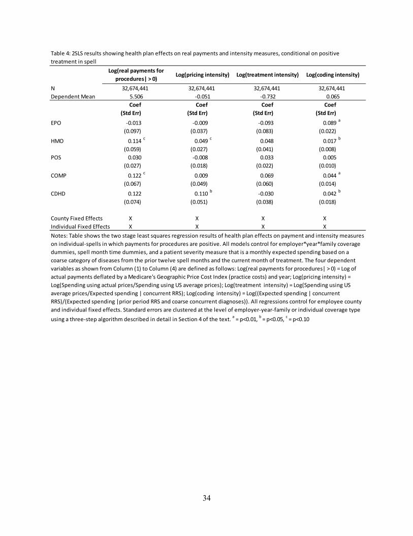
Section6.3:Plantypeeffecton(totalanddecomposed)healthcarespendingWe now examine how health plan types are associated with levels of health care spending and three intensity measures conditional on a patient deciding to make a visit.27

The 2SLS results are shown in Table 4.28 All regressions control for risk adjustment, spell time dummies, employer-year-family coverage fixed effects, and employee county and individual

25 See Appendix Table A-6 and A-7 for details on the first stage regression results. 26 OLS results in Appendix Table A-3 show that compared to PPOs, all other plans tend to discourage patients from making visits, regardless of whether these other plans feature a relatively higher cost sharing (like CDHDs) or more restrictive provider network (like EPOs and HMOs) or even higher generosity (like COMPs). 27 Our spending includes both patient out-of-pocket spending and plan payments. Although we estimated models of both total spending and spending on procedures, we prefer and focus our attention on the latter because facility payments are much harder to price and to predict, particularly when trying to calculate a national average price to use for generating normalized prices. Further justifications for using procedure payments can be found in Appendix B.3.

17

fixed effects.29 Results show that conditional on a visit, HMOs and COMPs are more expensive than PPOs. Neither EPOs nor CDHD plans are statistically significantly different from PPOs. The point estimate on CDHD plans is positive and suggests that costs are 12.2 percent higher than PPOs after controls, although not quite statistically significant (p = 0.101).

The decomposed regression results show that none of the plans particularly promote using lower price providers relative to PPOs. HMOs on average have 4.9 percent higher prices, and consumers among CDHDs face statistically 11.0 percent higher prices (p = 0.03) than in PPOs. In addition, none of the plan types show statistically significant effects on treatment intensity. The final column in Table 4 shows that all of the plan types code patients more intensively than PPOs (although the difference is not statistically significant for POS plans). Overall, about 15% (36%, 34%) of the 11.4% (12.2%, 12.2%) increase in procedure-related payments among HMOs (COMPs, CDHDs) relative to PPOs is contributed by differences in coding intensities.

Finally, we estimate the overall health plan type effects on health care spending (with a focus on procedure payments) by calculating expected total health spending as the product of visit rate (Pr(visit)) and total spending conditional on receiving care (Y|Y>0). To do this, we adopt a bootstrap approach that takes into account the empirical correlations between visit decisions and determination of spending conditional on receiving care (for example, consumers who are more likely to visit doctors are likely to pay more conditional on receiving care). Specifically, we re-estimate our full models on 100 random samples of our data drawn at employer-year-family coverage type (EYF) levels and generate confidence intervals from the empirical distribution of the predicted levels of treatment spells and spending in our sample using the sample mean for all PPO enrollees (our base plan type).30

Table 5 shows the bootstrapped means and 95% confidence intervals of probability of visit, procedure payments per spell (conditional and unconditional on a visit), and predicted total savings of each plan type relative to PPOs from our two part models.31, 32 Results imply that all

28 In an earlier version of this paper, we included provider fixed effects in our model which we now drop here. We made this change because (1) provider IDs are subject to serious missing values forcing us to drop a sizable fraction of our sample, and (2) there is reason to believe that the provider fixed effects may absorb some of the impact of plan incentives: one impact of changing plans and responding to higher cost sharing or restricted provider choice could be to switch to a lower cost provider. 29 For comparison, results with only employee county fixed effects or individual fixed effects are shown in Appendix Table A-4. We see that regressions with and without individual effects give very different predictions about plan type effects on the spending and intensity measures. Once individual fixed effects are controlled for, geographic variation does not explain much of the plan type effects on the total and decomposed procedure-related payments. 30 Further details about this method are described in Appendix C. 31 In Appendix Table A-8, we present results from conducting three different bootstrapping estimates of the results in Table 5. All of these predictions use the sample means of all control variables for PPO enrollees and predictions are presented by plan type. The first set of bootstrap estimates uses the EYF clustering from the base case of our analysis, in which we randomly select 100 draws of enrollees by EYF. The second simulation uses random draws of individuals but not EYF clusters, while the third set uses 100 two stage random sampling of both EYFs and individuals. These simulations show that estimated mean effects are robust to how bootstrapped samples are drawn, and that standard errors are only modestly higher when both EYF and individual level observation correlations are controlled for. Simulations while only correcting for individual error correlations underestimate standard errors relative to those allowing EYF error correlations. Results using two stage bootstrapping lead to similar conclusions about statistical significance as those used in our base case as presented here.

18

three narrow network plans (EPOs, HMOs, and POS plans) statistically significantly predict a reduced probability of a visit relative to PPOs.33 None of these three plan types achieve lower payments on procedures conditional on patients seeking care. Overall, none of these three plan types is successful in reducing overall health care expenditures relative to PPOs (final column). The bootstrapped estimates confirm that CDHDs do not differ statistically in their probability of any visit, and also suggest that they have higher spending conditional on a visit spell.34 Overall, both COMPs and CDHDs are predicted to increase total monthly spending on procedures relative to PPOs. The point estimate is that spending on procedures is $75 higher for COMPs and $36 higher for CDHDs. These reflect spending on procedures that is 34 percent higher for COMPs and 16 percent higher for CDHDs.35

Section7:DiscussionandconclusionsThis paper examines variation in health care utilization and spending for a monthly spell of treatment. Our results confirm the widely held finding that comprehensive insurance plans - which do not manage care, require gatekeepers, or restrict provider choices on the supply side and tend to have minimal cost sharing - have the highest procedure costs, enroll sicker patients, induce a higher probability of seeking care, and have higher costs conditional on making a visit. Narrow networks seem effective in reducing probability of visits, particularly new visits. Similarly to all other plan types, narrow network plan types do not differ meaningfully from PPOs in influencing decisions to seek continuing or chronic care.36 Using our decomposition framework to explain total spending on procedures, we find no effect of EPOs on prices or treatment intensity, but statistically significant increase in coding intensity relative to PPOs. In terms of total spending on procedures, EPOs appear to be the lowest cost plan type, but the difference from PPOs is not statistically significantly different from zero (p = 0.26). Among the limited evidence from previous studies, Gruber and McKnight (2014) examined insurance offerings to Massachusetts state employees which changed its health insurance. They found an overall 4.2% decline in total spending after the state provided incentives for enrolling in limited network plans. They report a 36% decline among enrollees who chose to switch to a limited network plan, but acknowledge that this is a self-selected group. A business study from the

32 Unlike previous estimation results, these bootstrapped results reflect an alternative way of calculating standard errors that are robust to clustered errors, and also permit calculations of predicted means in levels using all of the structural parameters in the model. Because bootstrapped estimates are calculated in a different manner, the statistical significance in Table 5 differs from that in the corresponding results in Table 3 column 1 and Table 4 column 1. This is both because bootstrapping uses empirical sampling distributions rather than analytical expressions for cluster-robust standard errors, and also because the confidence intervals used here are not symmetrical around the point estimate, as they are when using a normal distribution approximation for standard errors. We briefly mention differences in the text and discuss this issue further in Appendix C. 33 Note that in Table 3, EPOs were not statistically significantly different from PPOs in the probability of visit model. 34 Table 4 finds no significant effect of CDHDs on procedure spending. 35 In the appendix, we take a different approach and directly estimate the health plan type effects on both total payments and spending on procedures using the full analysis sample including spell months with zero payments. Results are shown in Table A-5. See a description of the alternative methodology used there. According to the table, EPO plans seem to achieve the most cost savings whereas comprehensive insurance has a consistently higher spending than PPOs. Table A-5 also shows that total spending that includes facility payments is more sensitive to outliers (e.g. Column 3 versus 6) than procedure payments where topcoding does not change the qualitative implications about plan types’ relative savings (e.g. Column 9 versus 12). 36 The only exception is HMO plans that are shown to reduce continuation visits relative to PPOs by 13 percent.

19

McKinsey Center for U.S. Health System Reform (2013) reports even larger premium savings of 21 percent from narrow relative to broad panel plans, although they do not mention controlling for selection effects. We do not know of any studies that examine the underlying reasons for cost savings in narrow panel plans such as EPOs.

Our most surprising result is that CDHDs are associated with 16 percent higher total spending on procedures relative to PPO plans (Table 5). The apparent cost savings of CDHDs relative to PPOs from comparing sample means and using OLS disappear once we control for endogenous plan type choice, patient severity of illness, and individual fixed effects, with the last adjustment making the biggest contribution. Note that we model spending that includes both health plan and out-of-pocket payments for procedures. Our decomposition of spending shows that this reflects a combination of no significant effect on rates of visits, 11 percent higher average prices, and 4 percent higher coding intensity conditional on a visit. Since CDHDs do not negotiate prices like PPOs, the plan type that has the greatest market share which may increase its bargaining power, it is not entirely surprising that people in CDHDs face higher prices relative to PPOs. Information available to consumers to enable them to shop around is improving, and may eventually introduce lower prices as market share and experience with CDHD plans grow. The current enthusiasm about CDHD plans saving money may arise because they shift expenses away from employers onto enrollees, and may serve to deter high risk enrollees. We are not aware of any previous studies of CDHDs that had panel data on 37 employers offering CDHDs, used risk adjustment and individual fixed effects, and controlled for endogenous plan choice when calculating cost savings. Future studies will hopefully apply similar careful control methods on alternative samples and aggregates of spending to validate or refine our findings.

Previous studies on consumer-driven and high-deductible health plans offer mixed evidence on the effectiveness of these plans in reducing utilization and spending due to selection bias, the short study period, and the modest sample of firms offering these plans. Parente and Feldman (2008) found lower health care costs for enrollees in CDHPs than in PPOs in initial enrollment years and but CDHPs rose to become the most expensive option in the follow-up year. Some of the most recent studies show evidence of more significant savings from CDHPs (Lo Sasso, Shah and Frogner 2010; Fronstin, Sepúlveda, and Roebuck 2013; Haviland et al. 2015).37

Perhaps the most directly comparable study to ours is one by Haviland et al. (2015) who, using the same data source as ours, compare the health care cost of enrollees in firms who first offer CDHPs alongside traditional plans with firms offering only traditional plans. They show that firms offering a CDHP had lower annual spending in the first three years post their offering but savings declined over the three year study period (6.6%, 4.3%, 3.4%). Our study is different from their study in several important ways. First, we use individual data rather than group means for our analysis, which enables us to control for individual characteristics, including both individual fixed effects and risk scores. Second, we examine costs of each plan type relative to PPOs, while Haviland et al. compare firms offering mixtures of different traditional plan types,

37 Lo Sasso, Shah and Frogner (2010) study a sample of 76,310 enrollees in 709 firms that switched from offering only traditional plans to offering an HSA-eligible plan exclusively or along with previously-offered traditional plans, and compare enrollees who switch to HSA-eligible plan to non-switchers. Fronstin, Sepúlveda, and Roebuck (2013) study one large firm who switched to offering CDHP exclusively that replaces PPO.

20

including not only PPOs but also HMOS, Comprehensive plans, and POS plans. Third, we only study health spending related to procedures and we do not include drug spending in our analysis.

Our results shed light on the complexity of designing policies to reduce health care spending through affecting demand- and supply-side incentives in several ways. First, supply-side plan designs such as selective provider contracting may be more effective in containing procedure-related costs than demand-side cost sharing. Second, although policies designed to either limit provider network or emphasize demand-side cost sharing may be effective in deterring new treatment where decisions are often dominated by patients, these policies are much less effective in influencing longer-term, repeated treatment where providers arguably play a bigger role. Third, due to potential interactions between various components of total spending (as in our decomposition), policies that are narrowly targeted may be counterproductive in reducing total costs if incentives to control one aspect of the spending create compensating effects/incentives in other aspects. For example, we show evidence that narrow network plans provide incentives to reduce provider contacts, but do so mostly for the less severely ill. Not only would this adverse selection increase average sickness of the remaining patients, it may also create an upcoding incentive for providers in these plans.

Our study is subject to several limitations. By using a continuous enrollee sample we exclude decedents and individuals of partial year eligibility. Since we have no information in this data set on death or other reasons why people drop out of the sample, we chose to restrict to a sample of population where non-random attrition is less of a concern. This paper studies only adults, excludes children and adults age 65 and over, and uses only age, gender, and diagnostic information for risk adjustment. Pharmacy information, and ideally consumer socioeconomic variables that affect access and information may also be important. We use “off the shelf” risk adjustment models but a more general approach would be to broaden the information available, and fully recalibrate models that predict each of our diverse outcomes.

Another limitation is that we do not observe premiums, benefit features, how narrow plan networks are or more generally measure heterogeneity of plan coverage within a plan type. Since we use employer-year-family coverage-plan type choice probabilities of instruments that capture this variation in plan type dummies, we do not believe that this introduces bias into our estimates of cost savings at the plan type level. But it does prevent us from measuring separately the cost saving impact of these specific plan feature dimensions.

A final limitation of our work is that by modeling aggregate spending, we end up aggregating diverse treatment decisions, diseases and providers. Many other studies also examine the effects of individual, provider, and plan characteristics on aggregates such as total spending, inpatient treatment and plan choice using even more aggregated approaches than ours, such as annual or county level spending (Glied 2000), but big data are making finer level analyses possible. Examination of disaggregated procedures, disease patterns, and treatment decisions, for which treatment spells are well suited, awaits further research.

21

References

Altman, Daniel, David M. Cutler, and Richard Zeckhauser. 2003. “Enrollee Mix, Treatment Intensity, and Cost in Competing Indemnity and HMO Plans.” Journal of Health Economics, 22(1): 23-45.

Anderson, Gerard F., Uwe E. Reinhardt, Peter S. Hussey, and Varduhi Petrosyan. 2003. “It’s The Prices, Stupid: Why The United States Is So Different From Other Countries.” Health Affairs, 22(3): 89-105.

Arondekar, Bhakti, Suellen Curkendall, Matthew Monberg, Beloo Mirakhur, Alan K. Oglesby, Gregory M. Lenhart, and Nicole Meyer. 2015. “Economic Burden Associated with Adverse Events in Patients with Metastatic Melanoma.” Journal of Managed Care and Specialty Pharmacy, 21(2): 158-64.

Aron-Dine, Aviva, Liran Einav, Amy Finkelstein, and Mark Cullen. 2015. “Moral Hazard in Health Economics: Do Dynamic Incentives Matter?” Review of Economics and Statistics. doi: 10.1162/REST_a_00518

Ash, Arlene S. and Randall P. Ellis. 2012. “Risk-Adjusted Payment and Performance Assessment for Primary Care.” Medical Care, 50(8): 643-653.

Ash, Arlene S., Randall P. Ellis, Gregory C. Pope, John Z. Ayanian, David W. Bates, Helen Burstin, Lisa I. Iezzoni, Elizabeth Mackay, Wei Yu. 2000. “Using Diagnoses to Describe Populations and Predict Costs.” Health Care Financing Review, 21(3): 7-28.

Bajari, Patrick, Christina Dalton, Han Hong, and Ahmed Khwaja. 2014. “Moral Hazard, Adverse Selection, and Health Expenditures: A Semiparametric Analysis.” The RAND Journal of Economics, 45(4): 747–763.

Baker, Laurence, Kate Bundorf, Anne Royalty, et al. 2007. “Consumer-Oriented Strategies for Improving Health Benefit Design: An Overview.” Rockville (MD): Agency for Healthcare Research and Quality (US); (Technical Reviews, No. 15.) Available from: http://www.ncbi.nlm.nih.gov/books/NBK44061/

Bonafede, Machaon M., Barbara H. Johnson, Madé Wenten, Crystal Watson. 2013. “Treatment Patterns in Disease-Modifying Therapy for Patients With Multiple Sclerosis in the United States.” Clinical Therapeutics, 35(10): 1501-1512.

Brachet, Tanguy. 2007. “Computing Clustered Standard Errors for Two-Stage Least Squares in SAS.” (software) http://works.bepress.com/tbrachet/2/.

22

Buchmueller, Thomas C. 2009. “Consumer-Oriented Health Care Reform Strategies: A Review of the Evidence on Managed Competition and Consumer-Directed Health Insurance.” Milbank Quarterly, 87: 820-841.

Bundorf, M. Kate. 2002. “Employee Demand for Health Insurance and Employer Health Plan Choices.” Journal of Health Economics. 21(1): 65–88.

Busch, Susan H. and Noelia Duchovny. 2005. “Family Coverage Expansions: Impact on Insurance Coverage and Health Care Utilization of Parents.” Journal of Health Economics, 24(5): 876-890.

Cameron, Colin and Douglas L. Miller. 2015. “A Practitioner’s Guide to Cluster-Robust Inference.” Journal of Human Resources, 50(2): 317-372.

Chernew, Michael E., Lindsay M. Sabik, Amitabh Chandra, Teresa B. Gibson, and Joseph P. Newhouse. 2010. “Geographic Correlation Between Large-Firm Commercial Spending and Medicare Spending.” American Journal of Managed Care, 16(2): 131–138.

Cutler, David, Jonathan Skinner, Ariel Dora Stern, and David Wennberg. May 2015. “Physician Beliefs and Patient Preferences: A New Look at Regional Variation in Health Care Spending.” Harvard Business School Working Paper, No. 15-090.

Deb, Partha and Pravin K. Trivedi. 2006. “Specification and Simulated Likelihood Estimation of a Non-normal Treatment-Outcome Model with Selection: Application to Health Care Utilization.” Econometrics Journal, 9(2): 307-331.

Dranove, David. 2000. “The Economic Evolution of American Health Care: From Marcus Welby to Managed Care.” Princeton: Princeton University Press.

Duarte, Fabian. 2012. “Price Elasticity of Expenditure across Health Care Services.” Journal of Health Economics, 31(6): 824-841.

Dugan, Jerome. 2014. “Trends in Managed Care Cost Containment: An Analysis of the Managed Care Backlash.” Health Economics. doi: 10.1002/hec.3115.

Eichner, Matthew J. 1998. “The Demand for Medical Care: What People Pay Does Matter.” American Economic Review, 88(2): 117-121.

Einav, Liran, Amy Finkelstein, Stephen P. Ryan, Paul Shrimpf, and Mark R. Cullen. 2013. “Selection on Moral Hazard in Health Insurance.” American Economic Review, 103(1): 178-219.

Einav, Liran, Amy Finkelstein, and Paul Schrimpf. 2015. “The Response of Drug Expenditure to Non-Linear Contract Design: Evidence from Medicare Part D.” The Quarterly Journal of Economics. doi: 10.1093/qje/qjv005

23

Ellis, Randall P. 1986. “Rational Behavior in the Presence of Coverage Ceilings and Deductibles.” The Rand Journal of Economics, 17(2): 158-175.

Ellis, Randall P., Siyi Luo, and Wenjia Zhu. 2015. “Multiple High Dimensional Fixed Effect Models in Health Economics.” Boston University working paper.

Federal Register. 2013. “Medicare and Medicaid Programs: Home Health Prospective Payment System Rate Update for CY 2014, Home Health Quality Reporting Requirements, and Cost Allocation of Home Health Survey Expenses.” 78 FR 72255 (2 December 2013): 72255-72320.

Fronstin, Paul; Martín J. Sepúlveda; M Christopher Roebuck. 2013. “Consumer-Directed Health Plans Reduce the Long-Term Use of Outpatient Physician Visits and Prescription Drugs.” Health Affairs, 32(6): 1126-1134.

Galbraith, Alison A., Stephen B. Soumerai, Dennis Ross-Degnan, Meredith B. Rosenthal, Charlene Gay, Tracy A. Lieu. 2012 “Delayed and Forgone Care for Families with Chronic Conditions in High-Deductible Health Plans.” Journal of General Internal Medicine, 27(9): 1105-1111.

Geruso, Michael and Timothy J. Layton. 2014. “Upcoding or Selection? Evidence from Medicare on Squishy Risk Adjustment.” Unpublished.

Glied, Sherry. 2000. “Managed Care.” in Handbook of Health Economics, edited by Anthony J. Culyer and Joseph P. Newhouse, 1A: 707–753. Amsterdam: North-Holland.

Gruber, Jonathan and Robin McKnight. 2014. “Controlling Health Care Costs Through Limited Network Insurance Plans: Evidence from Massachusetts State Employees.” NBER working paper series 20462, http://www.nber.org/papers/w20462

Haviland, Amelia M., Matthew D. Eisenberg, Ateev Mehrotra, Peter J. Huckfeldt, and Neeraj Sood. 2015. “Do “Consumer-Directed” Health Plans Bend the Cost Curve Over Time?” NBER working paper series 21031, http://www.nber.org/papers/w21031.

Hellinger, Fred J. 1995. “Selection Bias in HMOs and PPOs: A Review of the Evidence.” Inquiry, 32(2): 135-142.

Keeler, Emmett B., Willard G. Manning, and Kenneth B. Wells. 1988. “The Demand for Episodes of Mental Health Services.” Journal of Health Economics, 7(4): 369-392.

Keeler, Emmett B. and John E. Rolph. 1988. “The Demand for Episodes of Treatment in the Health Insurance Experiment.” Journal of Health Economics, 7(4): 337-367.

24

Keeler, Emmett B., John E. Rolph, Haihua Duan, Janet M. Hanley, Willard G. Manning. 1982. “The Demand for Episodes of Medical Treatment: Interim Results from the Health Insurance Experiment.” Santa Monica, CA: RAND Corporation; R-2829-HHS.

Keeler, Emmett B., Kenneth B.Wells, Willard G. Manning, J. David Rumpel, Janet M. Hanley. 1986. “The Demand for Episodes of Mental Health Services.” Santa Monica, CA: RAND Corporation, R-3432-NIMH.

Kowalski, Amanda. 2015. “Censored Quantile Instrumental Variable Estimates of the Price Elasticity of Expenditure on Medical Care.” Journal of Business & Economic Statistics, doi: 10.1080/07350015.2015.1004072.

Kronick, Richard and W. Pete Welch. 2014. “Measuring Coding Intensity in the Medicare Advantage Program.” Medicare & Medicaid Research Review, 4(2): E1-E19. http://www.cms.gov/mmrr/Downloads/MMRR2014_004_02_a06.pdf

Landon, Bruce E., Alan M. Zaslavsky, Robert C. Saunders, L. Gregory Pawlson, Joseph P. Newhouse and John Z. Ayanian. 2012. “Analysis Of Medicare Advantage HMOs Compared With Traditional Medicare Shows Lower Use Of Many Services During 2003–09.” Health Affairs, 31(12): 2609–2617.

Lorenzoni, Luca, Annalisa Belloni, and Franco Sassi. 2014. “Health-care Expenditure and Health Policy in the USA versus Other High-spending OECD Countries.” The Lancet. 384(9937): 83–92.

Lo Sasso, Anthony T., Mona Shah, and Bianca K. Frogner. 2010. “Health Savings Accounts and Health Care Spending.” Health Services Research, 45: 1041-1060.

MaCurdy, Thomas, Jason Kerwin, Jonathan Gibbs, et al. Acumen, LLC.: August 2008. “Evaluating the Functionality of the Symmetry ETG and Medstat MEG Software in Forming Episodes of Care Using Medicare Data.” Submitted to the Centers for Medicare and Medicaid Services, available at https://www.cms.gov/Research-Statistics-Data-and-Systems/Statistics-Trends-and-Reports/Reports/downloads/MaCurdy.pdf

Manning, Willard G, Joseph P. Newhouse, Naihua Duan, Emmett B. Keeler, and Arleen Leibowitz. 1987. “Health Insurance and the Demand for Medical Care: Evidence from A Randomized Experiment.” American Economic Review, 77(3): 251-277.

McKinsey Center for U.S. Health System Reform. 2013. “Hospital Networks: Configurations on the Exchanges and Their Impact on Premiums.” New York: McKinsey & Company. available at: http://healthcare.mckinsey.com/hospital-networks-configurations-exchanges-and-their-impact-premiums.

Meer, Jonathan and Harvey S. Rosen. 2004. “Insurance and the Utilization of Medical Services.” Social Science & Medicine, 58(9): 1623-1632.

25

Mello, Michelle M., Sally C. Stearns, Edward C. Norton and Thomas C. Ricketts III. 2003.

“Understanding Biased Selection in Medicare HMOs.” Health Services Research, 38(3): 961–992.

McKellar, Michael, Mary B. Landrum, Teresa Gilson, Bruce Landon, Sivia Naimer, and Michael Chernew. August 2012. “Geographic Variation in Health Care Spending, Utilization, and Quality among the Privately Insured.” Final Technical Report, presented to The Institute of Medicine Committee on “Geographic Variation in Health Care Spending and Promotion of High-Value Care”.

Newhouse, Joseph P. and Thomas G. McGuire. 2014. “How Successful Is Medicare Advantage?” The Milbank Quarterly, 92(2): 351-394.

Newhouse, Joseph P., J. Michael McWilliams, Mary Price, Jie Huang, Bruce Fireman, and John Hsu. 2013. “Do Medicare Advantage Plans Select Enrollees in Higher Margin Clinical Categories?” Journal of Health Economics, 32(6): 1278-1288.

Parente, Stephen T., Roger Feldman. 2008. “Evolution and Early Evidence of the Impact of Consumer-Driven Health Plans: From E-Commerce Venture to Health Savings Accounts.” Expert Review of Pharmacoeconomics and Outcomes Research, 8(4):343-348.

Peters, Rebecca and John Holahan. 2014. “Narrow Networks, Access to Hospitals and Premiums: An Analysis of Marketplace Products in Six Cities.” The Urban Institute Research Report, http://www.urban.org/research/publication/narrow-networks-access-hospitals-and-premiums-analysis-marketplace-products-six-cities/view/full_report. (Accessed 7/23/2015)

Romley, John A, Sarah Axeen, Darius N Lakdawalla, Michael E Chernew, Jay Bhattacharya, and Dana P. Goldman. 2015. “The Relationship between Commercial Health Care Prices and Medicare Spending and Utilization.” Health Services Research, 50(3): 883–896.

Rosen, Allison B., Eli Liebman, Ana Aizcorbe, and David M. Cutler. June 2012. “Comparing Commercial Systems for Characterizing Episodes of Care.” BEA working paper, available at http://www.bea.gov/papers/pdf/meg_vs_etg_paper.pdf

Steinwald, Bruce and Laura A. Dummit. 1989. “Hospital Case-Mix Change: Sicker Patients or DRG Creep?” Health Affairs, 8(2): 35-47.

Verisk Health, Inc. 2013. DxCG Intelligence User Guide v4.2.1, Waltham MA.

Wennberg, John E., Douglas O. Staiger, Sandra M. Sharp, Daniel J. Gottlieb, Gwyn Bevan, Klim McPherson, H. Gilbert Welch. 2013. “Observational Intensity Bias Associated with Illness

26

Adjustment: Cross Sectional Analysis of Insurance Claims.” British Medical Journal, 346: f549.

Wennberg, David E., Sandra M. Sharp, Gwyn Bevan, Jonathan S. Skinner, Daniel J. Gottlieb, John E. Wennberg. 2014. “A Population Health Approach to Reducing Observational Intensity Bias in Health Risk Adjustment: Cross Sectional Analysis of Insurance Claims.” British Medical Journal, 348 doi: http://dx.doi.org/10.1136/bmj.g2392.

27

28

Figure 2 Frequency of total health spending of spells following no visit for three time periods

0

5

10

15

20

25

0 500 1000 1500 2000 2500

Percent of sample

Total health spending costs

Annual

Calendar month

Spell month

Annual Calendar month Spell Months

N 1,543,207 42,356,547 37,931,381

Natural levels

Mean 3,248$ 658$ 789$

Std dev 14,957 4,262 4,725

CV 4.605 6.473 5.989

Topcoded at 99.9% at $250k at $50k at $50k

Mean 3,164$ 626$ 747$

Std dev 11,223 2,386 2,652

CV ‐ topcoded 3.547 3.813 3.548

Summary Statistics of New Visit Periods Using Annual,

Calendar Month and Spell Month Frameworks

29

Figure 3 Market shares of six health plan types in the analysis sample

Notes: Market shares are calculated at the patient level. Plan acronyms are defined in Table 1.

0%

10%

20%

30%

40%

50%

60%

2008 2009 2010 2011

Plan Type Share of Sample

1‐EPO

2‐HMO

3‐POS

4‐PPO

5‐COMP

6‐CDHD

30

Figure 4 Comparison of four standardized measures by plan type

Notes: For each plan type, the sample mean was divided by the overall sample mean in order to express as a standardized measure, which by construction has a grand mean of one. Relative risk scores are the prospective un-recalibrated DxCG risk scores predicting total health care spending in one month using only information from the prior twelve months (topcoded at $250,000). Plan acronyms are defined in Table 1.

0 0.2 0.4 0.6 0.8 1 1.2 1.4 1.6

EPO

HMO

POS

PPO

COMP

CDHD

Relative risk scores (RRS)

Any visit

Spending, topcoded

Spending on procedures, topcoded

31

Acronym Description Provider Network Cost Share (%)

EPOPatients must get care from in‐network

providers; gatekeeper; no capitation

Increasing choice

of providers6.2

HMOSame as EPO, but at least some services

are paid on capitated basis8.0

POSPatients have financial incentives to use

in‐network providers; gatekeeper11.0

PPOPatients have financial incentives to use

in‐network providers; no gatekeeper11.6

COMPNo limitations on patient use of any

particular providers9.6

CDHD

High deductible health plans with either a

Health Reimbursement or Health Savings

Account; no gatekeeper

16.1

Notes: Plan type descriptions (the first four columns) are based on 2011 Truven MarketScan Commercial Claims and

Encounters Database User’s Guide. Cost share in the last column is authors' calculation using the core analysis

sample (N=108,896,981) detailed in Section 5.1 and Appendix B.2. The measure captures the amount of total

payments paid by consumers. It is calculated by taking the ratio of patient out‐of‐pocket payments (i.e. sum of copay,

coinsurance, and deductible payments) to total spending that includes both patient out‐of‐pocket spending and plan

payments.

Table 1: Health plan type definitions and degrees of cost sharing and provider network generosity

Plan Type

Exclusive Provider

Organization

Health Maintenance

Organization

Point‐of‐Service,

noncapitated

Preferred Provider

Organization

Comprehensive

Consumer‐Driven/High

Deductible Health Plan

32

Plan Type AcronymN (person

spell‐months)

% of all

plan typesAge Male (%)

Relative

risk score

(RRS)

Any visit

indicator

Total real

payments,

topcoded

($)

Total real

procedure

payments,

topcoded

($)

Exclusive Provider Organization EPO 670,243 0.6% 46.0 48.1 1.089 0.334 $344 $227

Health Maintenance Organization HMO 26,099,610 24.0% 46.2 45.8 1.074 0.187 191 116

Point of Service POS 10,743,325 9.9% 46.4 43.7 1.098 0.308 330 185

Preferred Provider Organizations PPO 58,295,126 53.5% 47.0 48.0 1.177 0.348 357 223

Comprehensive COMP 2,734,967 2.5% 52.4 40.5 1.431 0.354 445 260

Consumer Directed Health Plan or

High Deductible Health PlanCDHD 10,353,710 9.5% 46.8 45.2 1.100 0.320 334 185

All plan types 108,896,981 100% 46.9 46.6 1.143 0.303 $315 $191

Table 2: Descriptive statistics on analysis sample

Notes: Data are from the MarketScan Commercial Claims and Encounter Data. The sample includes continuous enrollees over five

years during 2007‐2011, aged 21‐64, having at least one month of plan type information available during at least one month each

year, and to whom we an assign an employer (employers). The analysis sample drops 2007 data because they are used to predict

risk scores using diagnoses and/or demographics in the prior 12 months. Sample size is 108,896,981 person spell‐months. Relative

risk scores are calculated by prospective risk adjustment models predicting health care spending for 12 months (topcoded at

$250,000) prior to the current month. Any visit indicator equals to one if total spending in a spell month is positive. Both total and

procedure payments are topcoded at $50,000 per spell month. Refer to Appendix B for details on sample creation.

33

N

Dependent Mean

Coef Coef Coef Coef

(Std Err) (Std Err) (Std Err) (Std Err)

EPO ‐0.075 ‐0.064b

0.022 ‐0.018

(0.046) (0.031) (0.044) (0.030)

HMO ‐0.041a

‐0.013 ‐0.050a

‐0.027

(0.012) (0.012) (0.018) (0.021)

POS ‐0.024a

‐0.019b

‐0.012 0.003

(0.009) (0.008) (0.008) (0.018)

COMP 0.057b

0.075a

0.085a

0.004

(0.023) (0.021) (0.025) (0.034)

CDHD 0.011 0.020 0.014 0.022

(0.009) (0.014) (0.017) (0.017)

Table 3: 2SLS results showing health plan effects on probability of seeking unconditional visits

and three types of conditional visits

Pr(visits)Pr(V|N‐1) Pr(C|V‐1) Pr(C|C‐1)

New visits Continuation visits Chronic visits

Notes: Table shows the two stage least squares results from regressions at the individual‐spell

month level. Results show the effects of health plan on probability of seeking any care and

conditional on three previous spell types. All regressions control for employer*year*family

coverage dummies, spell month time dummies, a prospective model risk score predicting total

spending using the prior 12 spell months of diagnoses, and employee county and individual

fixed effects. Column (1) shows the probability of any visit regardless of the type of visit in

prior month. Column (2) correspond to the probability of new visit conditional on no visit in

previous month ("new visit" spells). Column (3) is the probability of continuing visit

conditional on a new visit in previous month ("continuation visit" spells). Column (4) denotes

the probability of continuing visit conditional on a previous continuation spell month of visit

("chronic visit" spells). Standard errors are clustered at the employer‐year‐family type

coverage level using a three‐step algorithm described in detail in Section 4 of the text. a =

p<0.01, b = p<0.05,

c = p<0.10

108,896,981 73,474,976 15,195,461 20,226,544

0.303 0.186 0.372 0.675

34

N

Dependent Mean

Coef Coef Coef Coef

(Std Err) (Std Err) (Std Err) (Std Err)

EPO ‐0.013 ‐0.009 ‐0.093 0.089a

(0.097) (0.037) (0.083) (0.022)

HMO 0.114c

0.049c

0.048 0.017b

(0.059) (0.027) (0.041) (0.008)

POS 0.030 ‐0.008 0.033 0.005

(0.027) (0.018) (0.022) (0.010)

COMP 0.122c

0.009 0.069 0.044a

(0.067) (0.049) (0.060) (0.014)

CDHD 0.122 0.110b

‐0.030 0.042b

(0.074) (0.051) (0.038) (0.018)

County Fixed Effects X X X X

Individual Fixed Effects X X X X

5.506 ‐0.051 ‐0.732 0.065

Notes: Table shows the two stage least squares regression results of health plan effects on payment and intensity measures

on individual‐spells in which payments for procedures are positive. All models control for employer*year*family coverage

dummies, spell month time dummies, and a patient severity measure that is a monthly expected spending based on a

coarse category of diseases from the prior twelve spell months and the current month of treatment. The four dependent

variables as shown from Column (1) to Column (4) are defined as follows: Log(real payments for procedures| > 0) = Log of

actual payments deflated by a Medicare's Geographic Price Cost Index (practice costs) and year; Log(pricing intensity) =

Log(Spending using actual prices/Spending using US average prices); Log(treatment intensity) = Log(Spending using US

average prices/Expected spending | concurrent RRS); Log(coding intensity) = Log((Expected spending | concurrent

RRS)/(Expected spending |prior period RRS and coarse concurrent diagnoses)). All regressions control for employee county

and individual fixed effects. Standard errors are clustered at the level of employer‐year‐family or individual coverage type

using a three‐step algorithm described in detail in Section 4 of the text. a = p<0.01,

b = p<0.05,

c = p<0.10

32,674,441 32,674,441 32,674,441 32,674,441

Table 4: 2SLS results showing health plan effects on real payments and intensity measures, conditional on positive

treatment in spell

Log(real payments for

procedures| > 0)Log(pricing intensity) Log(treatment intensity) Log(coding intensity)

35

mean 95% C.I mean 95% C.I mean 95% C.I mean 95% C.I

EPO 0.269b

(0.152, 0.342) 629 (511, 718) 172 (81, 241) ‐51 (‐142, 18)

HMO 0.307a

(0.285, 0.328) 724 (627, 826) 223 (187, 267) ‐1 (‐36, 44)

POS 0.324a

(0.312, 0.341) 664 (632, 700) 215 (201, 237) ‐8 (‐22, 14)

PPO 0.348 ‐ 647 ‐ 223 ‐ 0 ‐

COMP 0.408a

(0.375, 0.459) 731b

(649, 846) 298a

(258, 353) 75a

(35, 130)

CDHD 0.357 (0.342, 0.372) 727b

(649, 798) 259a

(230, 289) 36a

(7, 66)

Notes: Table shows the bootstrapped means and 95% confidence intervals of the visits and monthly real

procedure payments conditional on a visit from our two part models in Tables 3 (first column) and 4 (first

column). Results shown summarize the means and confidence intervals from estimating both models 100 times

on random samples of 108.9 million person spells with 510 employer‐year‐family coverage type combinations

drawn with replacement from the original sample. After first absorbing individual and county level fixed

effects, for each random sample we reestimate our full 2SLS models, to generate point estimates of the effects

of health plan types on the probability of a visit and spending conditional on a visit. Regression results from

each sample are then used to predict spending at the sample means of those who actually choose PPO plans.

Means for PPOs are calculated from the original sample. The 95% confidence interval corresponds to the 2.5 and

97.5 percentiles among the 100 simulated predictions. Estimates for monthly savings (the final two columns) are

obtained from the overall predictions in the earlier pair of columns by subtracting the predicted values for

PPOs from the other plan predictions. Significance letters show whether plan type predictions are statistically

significantly different from the PPO means based on the empirical bootstrapped distributions using two‐sided

tests: a = 1%,

b = 5%,

c = 10%.

Table 5: Bootstrapped (100 replications) 95% confidence intervals for any visit indicator, monthly spending,

expected spending, and expected savings relative to PPO plans by plan type

Any visit indicator

Monthly real

procedure payments|

> 0 ($)

Predicted monthly real

procedure payments ($)

Monthly savings

relative to PPOs ($)

36

AppendixA:Additionaltables

Period t‐1 spell types No Visit (N) New Visit (V) Continuation (C)

No Visit (N‐1) 1 ‐ Pr(V|N‐1) Pr(V|N‐1) 0

New Visit (V‐1) 1 ‐ Pr(C|V‐1) 0 Pr(C|V‐1)

Continuation (C‐1) 1 ‐ Pr(C|C‐1) 0 Pr(C|C‐1)

All Pr(N) Pr(V) Pr(C)

Table A‐1: Spell transition probabilities

Period t spell types

Notes: Lagged information is indicated by subscript ‐1, with N, V, and C denoting no

visit, new visit, and continuation spells, respectively.

Mean (Std Dev) Mean (Std Dev)

Age 46.9 (9.7) 46.9 (9.5)

Male (%) 46.6 (49.9) 46.6 (49.9)

Relative risk score (RRS) 1.208 (1.311) 1.143 (1.219)

Total real payments, topcoded $354 ($2,182) $315 ($2,032)

Total real procedure payments, topcoded $226 ($1,153) $191 ($1,006)

N (person spell‐months)

Table A‐2: Descriptive statistics on two estimation samples

Notes: Samples are from the MarketScan Commercial Claims and Encounter Data. The full

5M sample selects people who are: adults age 21 to 64, enrolled for 60 months during

2007 to 2011, non‐missing age, gender, region, and have at least one month of plan type

information in any year over the sample period. The analysis sample further selects spell

months to which we can assign an employer and health plan type, with additional sample

selection criteria imposed as detailed in Appendix B. In both samples, data from 2007 are

dropped to calculate relative risk score (RRS) predicting spending from 12 months prior to

the current month. Variables are defined the same way as in Table 2. Standard deviations

are in parentheses.

Full 5M sample Analysis sample

108,896,981245,824,416

37

N

Dependent Mean

Coef Coef Coef Coef Coef Coef Coef Coef

(Std Err) (Std Err) (Std Err) (Std Err) (Std Err) (Std Err) (Std Err) (Std Err)

EPO ‐0.008a

‐0.008a

‐0.003c

‐0.003c

‐0.007b

‐0.007b

‐0.005b

‐0.006b

(0.002) (0.002) (0.002) (0.002) (0.003) (0.003) (0.003) (0.003)

HMO ‐0.034a

‐0.034a

‐0.026a

‐0.026a

‐0.035a

‐0.035a

‐0.037a

‐0.037a

(0.008) (0.008) (0.006) (0.006) (0.010) (0.010) (0.009) (0.009)

POS ‐0.018a

‐0.017a

‐0.015a

‐0.015a

‐0.012a

‐0.011a

‐0.008b

‐0.008b

(0.005) (0.005) (0.004) (0.004) (0.004) (0.004) (0.003) (0.003)

COMP ‐0.015b

‐0.015b

‐0.007 ‐0.007 ‐0.017a

‐0.017a

‐0.015b

‐0.015b

(0.007) (0.007) (0.005) (0.005) (0.006) (0.006) (0.008) (0.008)

CDHD ‐0.015a

‐0.015a

‐0.012a

‐0.012a

‐0.012a

‐0.012a

‐0.008b

‐0.008b

(0.003) (0.003) (0.002) (0.002) (0.004) (0.004) (0.004) (0.004)

Risk Adjustment NO YES NO YES NO YES NO YES

Table A‐3: OLS results showing health plan effects on probability of seeking unconditional visits and three types of conditional

visits

Pr(visits)Pr(V|N‐1) Pr(C|V‐1) Pr(C|C‐1)

New visits Continuation visits Chronic visits

(7) (8)

108,896,981 73,474,976 15,195,461 20,226,544

(1) (2) (3) (4) (5) (6)

0.303 0.186 0.372 0.675

Notes: Table shows the OLS results from regressions at the individual‐spell month level. Results show the effects of health plan

on probability of seeking any care and conditional on three previous spell types. All the models control for

employer*year*family coverage dummies and spell month time dummies, and employee county and individual fixed effects.

Column (1) and (2) model the probability of any visit regardless of the types of visit in prior spell month. Column (3) through (4)

correspond to the probability of new visit conditional on no visit in previous month ("new visit" spells). Column (5) to (6) are the

probability of continuing visit conditional on a new visit in previous month ("continuation visit" spells). Column (7) to (8) denote

the probability of continuing visit conditional on a previous continuation spell month of visit ("chronic visit" spells). Within each

type of visit (conditional or unconditional), the second column differs from the first column in that it additionally controls for a

prospective model risk score predicting total spending using the prior 12 spell months of diagnoses ("Risk Adjustment").

Standard errors are clustered at the employer‐year‐family type coverage level using a three‐step algorithm described in detail

in Section 4 of the text. a = p<0.01,

b = p<0.05,

c = p<0.10

38

(1) (2) (3) (4) (5) (6) (7) (8)

N

Dependent Mean

Coef Coef Coef Coef Coef Coef Coef Coef

(Std Err) (Std Err) (Std Err) (Std Err) (Std Err) (Std Err) (Std Err) (Std Err)

EPO 0.473c

‐0.017 0.024 ‐0.011 0.668b

‐0.095 ‐0.220 0.090a

(0.249) (0.102) (0.064) (0.039) (0.321) (0.086) (0.187) (0.023)

HMO 0.271a

0.114c

0.046 0.052c

0.661a

0.043 ‐0.436a

0.019b

(0.063) (0.061) (0.033) (0.028) (0.095) (0.042) (0.062) (0.009)

POS ‐0.040 0.030 ‐0.058 ‐0.009 0.153a

0.034 ‐0.135a

0.006

(0.044) (0.028) (0.036) (0.018) (0.039) (0.023) (0.033) (0.011)

COMP 0.070 0.120c

‐0.007 0.011 ‐0.100b

0.067 0.177a

0.042a

(0.045) (0.071) (0.026) (0.051) (0.045) (0.063) (0.036) (0.014)

CDHD ‐0.030 0.129c

‐0.004 0.113b

0.042 ‐0.025 ‐0.068 0.042b

(0.024) (0.077) (0.014) (0.053) (0.092) (0.040) (0.085) (0.019)

County Fixed Effects X X X X

Individual Fixed Effects X X X X

5.506 ‐0.051 ‐0.732 0.065

Notes: Table shows the two stage least squares regression results of health plan effects on payment and intensity measures on

individual‐spells in which payments for procedures are positive. All models control for employer*year*family coverage dummies,

spell month time dummies, and a patient severity measure that is a monthly expected spending based on a coarse category of

diseases from the prior twelve spell months and the current month of treatment. The four dependent variables are defined as

follows: Log(real payments for procedures| > 0) = Log of actual payments deflated by a Medicare's Geographic Price Cost Index

(practice costs) and year; Log(pricing intensity) = Log(Spending using actual prices/Spending using US average prices); Log(treatment

intensity) = Log(Spending using US average prices/Expected spending | concurrent RRS); Log(coding intensity) = Log((Expected

spending | concurrent RRS)/(Expected spending |prior period RRS and coarse concurrent diagnoses)). The odd columns control for

employee county fixed effects, and the even columns control for enrollee fixed effects. Standard errors are clustered at the level of

employer‐year‐family or individual coverage type using a three‐step algorithm described in detail in Section 4 of the text. a = p<0.01,

b

= p<0.05, c = p<0.10

32,674,441 32,674,441 32,674,441 32,674,441

Table A‐4: 2SLS results showing health plan effects on real payments and intensity measures, conditional on positive treatment in

spell

Log(real payments for

procedures| > 0)Log(pricing intensity) Log(treatment intensity) Log(coding intensity)

39

OLS no RA OLS w. RA 2SLS w. RA OLS no RA OLS w. RA 2SLS w. RA

(1) (2) (3) (4) (5) (6)

N

Dependent Mean 337.78 314.56

Coef Coef Coef Coef Coef Coef

(Std Err) (Std Err) (Std Err) (Std Err) (Std Err) (Std Err)

EPO ‐1.64 ‐3.98 48.24 ‐0.57 ‐2.77 5.40

(7.18) (7.08) (97.41) (5.80) (5.60) (64.35)

HMO ‐44.24a

‐42.60a

127.46a

‐41.37a

‐39.83a

57.14

(8.76) (8.06) (49.28) (7.55) (6.97) (36.09)

POS ‐11.59 ‐7.96 ‐77.17a

‐12.83c

‐9.40 ‐75.16a

(7.17) (6.36) (28.68) (6.42) (5.72) (20.82)

COMP 22.69 21.80 337.74a

12.14 11.30 197.59b

(16.43) (15.02) (106.59) (13.40) (12.10) (77.48)

CDHD 0.27 1.71 ‐52.10 0.35 1.71 ‐25.77

(6.91) (6.01) (56.58) (5.52) (4.79) (38.93)

County Fixed Effects X X X X X X

Individual Fixed Effects X X X X X X

(7) (8) (9) (10) (11) (12)

N

Dependent Mean 192.00 191.01



EPO 28.14a

26.91a

‐93.04 27.99a

26.79a

‐88.28

(9.28) (9.39) (100.41) (9.39) (9.50) (96.75)

HMO ‐19.78a

‐18.92a

34.13 ‐19.31a

‐18.47a

31.89

(5.08) (4.72) (31.89) (5.02) (4.67) (29.87)

POS ‐28.64a

‐26.73a

‐21.94 ‐28.03a

‐26.17a

‐18.81

(10.04) (10.13) (16.71) (10.05) (10.14) (16.68)

COMP 1.67 1.20 123.97a

1.34 0.88 113.02a

(6.94) (6.57) (40.73) (6.94) (6.57) (38.88)

CDHD ‐2.15 ‐1.39 ‐8.57 ‐2.00 ‐1.26 ‐4.42

(3.65) (3.12) (18.05) (3.56) (3.06) (16.95)

County Fixed Effects X X X X X X

Individual Fixed Effects X X X X X X

108,896,981 108,896,981

Notes: Table shows the regression results of health plan effects on the four measures of real payments at the level of

person spell‐months, using the full analysis sample with spells of zero payments included. The four dependent variables

are: Real payments = Actual payments deflated by a Medicare's Geographgic Price Cost Index (practice costs) and year; Real

payments topcoded at $50,000/month; Procedure‐related (non‐facility) real payments; Procedure‐related (non‐facility)

real payments topcoded at $50,000/month. The three columns of each dependent variable correspond to the models of (1)

OLS without risk adjustment, (2) OLS with risk adjustment, and (3) 2SLS with risk adjustment. The risk adjustment uses a risk

score generated for each person spell‐month based on a prospective model predicting total spending using the prior 12

spell months of diagnoses. All models control for employer*year*family coverage dummies, spell month time dummies,

and employee county and individual fixed effects. Standard errors are clustered at the employer‐year‐family coverage

level using a three‐step algorithm described in detail in Section 4 of the text. a = p<0.01,

b = p<0.05,

c = p<0.10

Table A‐5: Alternative models of unconditional spending

Real payments Real payments topcoded at $50,000/mo

108,896,981 108,896,981

Real payments for proceduresReal payments for procedures topcoded

at $50,000/mo

40

Panel A: All visits Coef Coef Coef Coef Coef Coef

N=108,896,981 (Std Err) (Std Err) (Std Err) (Std Err) (Std Err) (Std Err)

EPOprob 1.010a

‐0.162a

‐0.388a

‐0.056a

‐0.313a

‐0.090a

(0.004) (0.010) (0.007) (0.004) (0.009) (0.013)

HMOprob 0.004 0.611a

‐0.400a

0.001 ‐0.201a

‐0.015

(0.004) (0.010) (0.006) (0.004) (0.009) (0.012)

POSprob 0.001 ‐0.068a

0.536a

‐0.048a

‐0.302a

‐0.119a

(0.004) (0.010) (0.006) (0.004) (0.008) (0.012)

COMPprob 0.000 ‐0.071a

‐0.389a

0.486a

‐0.251a

0.224a

(0.004) (0.010) (0.006) (0.004) (0.008) (0.012)

CDHprob 0.001 ‐0.048a

‐0.419a

‐0.035a

0.289a

0.211a

(0.004) (0.010) (0.006) (0.004) (0.008) (0.012)

HDHprob 0.017a

‐0.088a

‐0.401a

‐0.121a

0.515a

0.079a

(0.004) (0.010) (0.006) (0.004) (0.009) (0.012)

PPOprob 0.002 ‐0.095a

‐0.409a

‐0.019a

‐0.266a

0.786a

(0.004) (0.010) (0.006) (0.004) (0.008) (0.012)

F‐statistics 21432.1 76247.3 233259.0 22296.8 69814.5 148013.0

Panel B: New visits Coef Coef Coef Coef Coef Coef


EPOprob 1.027a

‐0.146a

‐0.289a

‐0.035a

‐0.405a

‐0.152a

(0.005) (0.012) (0.008) (0.005) (0.011) (0.015)


‐0.285a

0.016a

‐0.270a

‐0.066a

(0.005) (0.012) (0.008) (0.004) (0.010) (0.015)

POSprob 0.001 ‐0.088a

0.616a

‐0.027a

‐0.366a

‐0.136a

(0.004) (0.012) (0.008) (0.004) (0.010) (0.014)

COMPprob ‐0.001 ‐0.076a

‐0.273a

0.482a

‐0.338a

0.207a

(0.005) (0.012) (0.008) (0.004) (0.010) (0.015)

CDHprob 0.000 ‐0.059a

‐0.302a

‐0.018a

0.196a

0.183a

(0.005) (0.012) (0.008) (0.004) (0.010) (0.015)

HDHprob 0.013a

‐0.095a

‐0.285a

‐0.111a

0.424a

0.053a

(0.005) (0.012) (0.008) (0.004) (0.010) (0.015)

PPOprob 0.001 ‐0.105a

‐0.291a

0.004 ‐0.328a

0.720a

(0.004) (0.012) (0.008) (0.004) (0.010) (0.015)

F‐statistics 14815.5 51554.0 165296.0 16357.5 47997.2 102472.0

Table A‐6: First stage results of the 2SLS models showing health plan effects on probability of seeking any visit and three

types of visits

EPO CDHD PPOHMO POS COMP

41

Panel C: Continuation visits Coef Coef Coef Coef Coef Coef


EPOprob 0.992a

‐0.166a

‐0.485a

‐0.044a

‐0.372a

0.075b

(0.011) (0.028) (0.018) (0.011) (0.024) (0.035)


‐0.514a

0.009 ‐0.243a

0.089a

(0.010) (0.027) (0.017) (0.010) (0.023) (0.033)

POSprob 0.001 ‐0.042 0.447a

‐0.045a

‐0.352a

‐0.009

(0.010) (0.027) (0.017) (0.010) (0.023) (0.033)

COMPprob 0.002 ‐0.047c

‐0.504a

0.517a

‐0.298a

0.330a

(0.010) (0.027) (0.017) (0.010) (0.023) (0.033)

CDHprob 0.002 ‐0.023 ‐0.531a

‐0.027a

0.240a

0.340a

(0.010) (0.027) (0.017) (0.010) (0.023) (0.033)

HDHprob 0.021b

‐0.073a

‐0.510a

‐0.093a

0.463a

0.192a

(0.010) (0.028) (0.017) (0.011) (0.024) (0.034)

PPOprob 0.003 ‐0.072a

‐0.519a

‐0.015 ‐0.314a

0.916a

(0.010) (0.027) (0.017) (0.010) (0.023) (0.033)

F‐statistics 2959.7 10888.3 34524.3 3051.0 10023.5 22005.4

Panel D: Chronic visits Coef Coef Coef Coef Coef Coef


EPOprob 0.914a

‐0.217a

‐0.669a

‐0.081a

‐0.040c

0.092a

(0.010) (0.026) (0.017) (0.012) (0.022) (0.033)


‐0.713a

‐0.012 0.022 0.130a

(0.010) (0.025) (0.017) (0.012) (0.021) (0.032)

POSprob 0.002 ‐0.035 0.282a

‐0.070a

‐0.102a

‐0.077b

(0.010) (0.025) (0.016) (0.012) (0.021) (0.032)


‐0.708a

0.519a

‐0.015 0.283a

(0.010) (0.025) (0.017) (0.012) (0.021) (0.032)

CDHprob 0.004 ‐0.043 * ‐0.738a

‐0.035a

0.611a

0.200a

(0.010) (0.025) (0.017) (0.012) (0.021) (0.032)

HDHprob 0.024b

‐0.084a

‐0.725a

‐0.097a

0.706a

0.176a

(0.010) (0.025) (0.017) (0.012) (0.022) (0.032)

PPOprob 0.006 ‐0.090a

‐0.735a

‐0.045a

‐0.083a

0.946a

(0.010) (0.025) (0.017) (0.012) (0.021) (0.032)

F‐statistics 3779.5 14339.0 37815.7 3631.2 12462.9 25459.3

Notes: Table reports the first stage regressions of the 2SLS models showing health plan effects on probability of visits,

with one regression for each of the six endegenous plan types shown as separate columns. The instruments are

probabilities of choosing plan types (shown in rows) predicted from multinomial logit models at the household‐year

level. The probabilities of two consumer‐driven health plan types ‐ consumer‐driven health plan (CDH) and high‐

deductible health plan (HDH) ‐ were predicted separately in multinomial logit models, and thus both were used as

instruments. Other exogenous control variables include a prospective model risk score in household predicting total

spending using the prior 12 spell months of diagnoses, employee county and individual fixed effects, employer‐year‐

family coverage fixed effects, and spell month fixed effects. Panel A reports the regression results using all spells of

treatment ("All visits"). Panel B through D run regressions on subsets of samples. Specifically, Panel B is based on

regressions using only spells following no prior visits ("New visits"). Panel C focuses on spells of treatment that follow a

new visit in the previous spell ("Continuation visits"). Panel D corresponds to models using all the spells preceded by a

continuation visit ("Chronic visits"). a = p<0.01,

b = p<0.05,

c = p<0.10

Table A‐6 (Continued): First stage results of the 2SLS models showing health plan effects on probability of seeking any

visit and three types of visits

EPO HMO POS COMP CDHD PPO

42



EPOprob 0.946a

‐0.204a

‐0.574a

‐0.057a

‐0.189a

0.078a

(0.008) (0.019) (0.013) (0.008) (0.017) (0.024)


‐0.614a

0.003 ‐0.097a

0.086a

(0.007) (0.018) (0.012) (0.008) (0.016) (0.024)

POSprob 0.001 ‐0.046b

0.379a

‐0.054a

‐0.221a

‐0.058b

(0.007) (0.018) (0.012) (0.008) (0.016) (0.023)


‐0.608a

0.523a

‐0.140a

0.292a

(0.007) (0.018) (0.012) (0.008) (0.016) (0.024)

CDHprob 0.002 ‐0.043b

‐0.637a

‐0.027a

0.433a

0.271a

(0.007) (0.018) (0.012) (0.008) (0.016) (0.024)

HDHprob 0.023a

‐0.087a

‐0.617a

‐0.090a

0.597a

0.174a

(0.007) (0.019) (0.012) (0.008) (0.016) (0.024)

PPOprob 0.003 ‐0.090a

‐0.629a

‐0.026a

‐0.191a

0.933a

(0.007) (0.018) (0.012) (0.008) (0.016) (0.023)

F‐statistics 6276.9 23907.2 67413.6 6003.3 20877.2 45257.2

N 32,674,441 32,674,441 32,674,441 32,674,441 32,674,441 32,674,441

Notes: Table reports the first stage regressions of the 2SLS models showing health plan effects on real payments and

intensity measures, with one regression for each of the six endegenous plan types shown as separate columns. The

instruments are probabilities of choosing plan types (shown in rows) predicted from multinomial logit models at the

household‐year level. The probabilities of two consumer‐driven health plan types ‐ consumer‐driven health plan (CDH)

and high‐deductible health plan (HDH) ‐ were predicted separately in multinomial logit models, and thus both were

used as instruments. Other exogenous control variables include a patient severity measure that is a monthly expected

spending based on a coarse category of diseases from the prior twelve spell months and the current month of

treatment, employee county and individual fixed effects, employer‐year‐family coverage fixed effects, and spell month

fixed effects. Sample size is 32,674,441 including all spells in which individuals are treated and incur positive payments

on medical services. a = p<0.01,

b = p<0.05,

c = p<0.10

Table A‐7: First stage results of the 2SLS models showing health plan effects on real payments and intensity measures,

conditional on a visit in spell

EPO HMO POS COMP CDHD PPO

43

Model A: Random sampling of EYFs


EPO 0.269b(0.152, 0.342) 629 (511, 718) 172 (81, 241) ‐51 (‐142, 18)

HMO 0.307a(0.285, 0.328) 724 (627, 826) 223 (187, 267) ‐1 (‐36, 44)

POS 0.324a(0.312, 0.341) 664 (632, 700) 215 (201, 237) ‐8 (‐22, 14)

PPO 0.348 ‐ 647 ‐ 223 ‐ 0 ‐

COMP 0.408a(0.375, 0.459) 731

b(649, 846) 298

a(258, 353) 75

a(35, 130)

CDHD 0.357 (0.342, 0.372) 727b

(649, 798) 259a(230, 289) 36

a(7, 66)

Model B: Random sampling of individuals


EPO 0.270a(0.247, 0.291) 637 (574, 703) 172

a(149, 195) ‐51

a(‐74, ‐28)

HMO 0.306a(0.296, 0.314) 726

a(695, 755) 222 (208, 234) ‐1 (‐15, 11)

POS 0.324a(0.317, 0.331) 668

b(650, 692) 216 (208, 225) ‐7 (‐15, 2)

PPO 0.348 ‐ 647 ‐ 223 ‐ 0 ‐

COMP 0.405a(0.389, 0.421) 734

a(692, 783) 297

a(273, 323) 74

a(50, 100)

CDHD 0.360a(0.350, 0.369) 732

a(703, 758) 263

a(250, 274) 40

a(27, 51)

Model C: Random sampling of EYFs and individuals


EPO 0.268c(0.149, 0.359) 629 (511, 718) 171 (84, 263) ‐52 (‐139, 40)

HMO 0.306a(0.285, 0.332) 725 (628, 840) 222 (183, 270) ‐1 (‐40, 47)

POS 0.324b(0.307, 0.347) 665 (618, 711) 215 (199, 241) ‐8 (‐24, 18)

PPO 0.348 ‐ 647 ‐ 223 ‐ 0 ‐

COMP 0.407a(0.364, 0.457) 730 (617, 858) 297

a(249, 371) 74

a(26, 148)

CDHD 0.358 (0.339, 0.376) 727b

(656, 813) 260a(230, 289) 37

a(7, 66)

Notes: Table shows results from conducting three different bootstrapping estimates of the results

in Table 5. The first set of bootstrap estimates (Model A) uses the EYF clustering in which we

randomly conducted 100 draws of EYFs and include in sample all enrollee‐spells within each

selected EYF. This replicates the results presented in Table 5. The second simulation (Model B)

uses random draws of individuals but not EYF clusters, while the third set of estimates (Model C)

uses 100 two stage random sampling of both EYFs and individuals. All of these predictions are

presented by plan type and use the sample means of all control variables for PPO enrollees. Means

for PPOs are calculated from the original sample. The 95% confidence interval corresponds to the

2.5 and 97.5 percentiles among the 100 simulated predictions. Estimates for monthly savings (the

final two columns) are obtained from the overall predictions in the earlier pair of columns by

subtracting the predicted values for PPOs from the other plan predictions. Significance letters

show whether plan type predictions are statistically significantly different from the PPO means

based on the empirical bootstrapped distributions using two‐sided tests: a = 1%,

b = 5%,

c = 10%.

Predicted monthly

real procedure

payments ($)

Monthly savings

relative to PPOs

($)

Table A‐8: 95% confidence intervals from three bootstrap models (100 replications) for any visit

indicator, monthly spending, expected spending, and expected savings relative to PPO plans by

plan type

Any visit indicator

Monthly real

procedure

payments| > 0 ($)

44

AppendixB:DataprocessingB.1DealingwithmissinginformationB.1.1MissingemployersThe Truven Health Analytics MarketScan® (MS) Commercial Claims and Encounter data has two kinds of claims, those originating from employers and those originating from health plans. Health plan identifiers (“plan key”), which also identify employers, are only provided on a subset of the employer sample, and only for a subset of each employer’s years. Since a key feature of the MS employer data is that when an enrollee changes employers, his enrollee ID will change, we can reliably infer that if a person is in the sample for all five years, then that household is almost always associated with the same employer (or affiliate if there is a merger or breakup). Hence for each household in the employer sample we assigned the employer from a previous or subsequent year. This roughly quadrupled our sample with an employer assigned. B.1.2MissingplankeysAs summarized in the Table 1, the MS data contains a diverse set of different health plan types that we wish to include. Health plan identifiers (“plan key”) that index a specific plan are missing on 75.9% percent of the eligibility records, and are only present for all five years on 5.3% of all enrollees. However, health plan type is provided for over 98% of all enrollees, and is present for all five years on 97% of the records. We conducted an analysis of plan IDs and plan types and determined that where plankey is present, employers on average offer 2.03 plankey ID for each given plan type offered that year. Employers are more likely to offer multiple PPOs, HMOs and POS, the three most common plan types, and less likely to offer multiple EPO, CDHD plans if they offer these plan types at all. We conduct our analysis at the employer*year*family coverage*plan type level instead of the unique plan key level. While this blurs the distinction among distinct HMO, PPO, POS plans of the same plan type, it preserves a large sample size, and the distortion on the two newest plan types, EPOs and CDHDs, is small. B.1.3MissingemployeecountiesBeginning in 2011, MS no longer includes employee county in their data. After determining that the annual migration rates during 2007 to 2010 in our 5.1 million continuously eligible sample are less than 3%, we impute the missing county information in 2011 by corresponding values in 2010, the last year such information is available. This imputation intrudes some measurement error but only affects the results where county fixed effects are used. B.2SampleselectiondetailsOur 5.1 million sample includes individuals aged 21-64, enrolled continuously for 60 months during 2007-2011, and having at least one month of plan type information available during at least one month of each year. Records with missing enrollee IDs, age, or sex were excluded. To construct analysis sample, we excluded all spells in which we detect any payments based on capitation where payments are likely understated. This includes all spells associated with a plan type called “Point of Service with Capitation”, and spells involving capitation payments (mostly in PPO and POS plans). Since primary care during pregnancies will differ from care at other times, we excluded all spells in which there was a pregnancy diagnosis, both concurrently or during the prior twelve month base period in which diagnoses are recognized for each spell.

45

The first 12 spell months (from 2007) are dropped because they are used to predict risk scores using diagnoses and/or demographics in the prior twelve months. We also dropped the last spell in our sample (i.e. spell index = 60) because it will be truncated from continuation into 2012. Analysis sample for analyzing procedure-related payments and intensities further restricts our sample to spells with positive sum of procedure payments (in both nominal and real terms). B.3PricedeflationIn order to distinguish price variation that is explained by provider choice from price variation due to time trends and cost of living, prices on each claim were first deflated by an inflation adjustment (using 2011 dollars) which normalized the average price to be constant in all years, and then normalized prices by dividing by the county or state prices as captured by the Medicare programs Geographic Practice Cost Index (GPCI) as used in the physician time component of the Medicare Part B payments. The practice expense GPCI reflects regional differences in the wages of employees in physician practices, such as nurses and office staff, and differences in median residential rents, which serve as a proxy for office rent. Quantities of services on each claim were multiplied by these real prices to calculate the value of real payments. This means that our real health expenditures control for both time and geographic price variation. In addition to deflating all expenditures to be in real, time and county adjusted prices, we also calculate national average prices separately for each procedure code, and also for classes of non-procedure claim (e.g. facility payments) so that the national average prices could be multiplied by actual quantities to generate a measure of what prices would have been if the US average payments were used. The pricing intensity of a spell is the real price for the set of services provided, divided by what the payment would have been if the US average prices instead of the providers own prices are used. Both payments are calculated using the actual quantities of services received. Since the measuring units of facility services (hospital days, DRGs, time receiving tests, days of care, hours in an ICU, etc.) are not as readily captured as counts of procedures, there is reason to believe the US average payments for procedures are a more accurate payment measure than US average payments that include facility payments. Hence our preferred dependent variable focuses on real payments for procedures, rather than total real payments including both procedures and facility payments.

B.4RiskadjustmentRisk adjustment models have gained increasing attention in the US in the past fifteen years with their expanded use for paying Medicare Advantage, Medicaid managed care plans, Medicare Part D, and the ACA’s new Health Insurance Marketplace. The age, gender and diagnoses of an individual over any base period have been shown to be important predictors of many outcomes, notably including both concurrent models in which diagnoses are used to predict spending in the same base period as the diagnoses are observed, and prospective models in which spending and utilization are predicted using diagnoses from a previous base period (Ash et al. 2000).

We use diagnosis-based risk adjustment models in four ways in this paper: to capture patient illness burdens when modeling employee choice of health plans; to capture illness burdens when consumers decide to make a visit; to control for patient severity in treatment decisions; and to quantify coding intensity variation. Spell month treatment decisions are modeled as depending on various combinations of concurrent and prior period diagnoses.

46

We use used DxCG models to generate predictions using eligibility, age, sex and diagnostic information which enabled us to estimate separate models using both coarse (simplified) and fine (rich) diagnostic detail. For modeling health plan choice and visit decisions, we use diagnoses from the prior year to generate a prospective, rich Hierarchical Condition Category (HCC) classification system that expands upon the system used for the Medicare Advantage and Marketplace programs and distinguishes between 384 HCCs. For overall severity entering the denominator of the coding intensity measure and treatment decisions, we use DxCG’s relatively coarse Related Condition Categories (RCCs) for prediction. The 117 RCCs approximate the level of details that most consumers will have, and are similar to conditions appearing on household surveys such as the Medical Expenditure Panel Survey (MEPS) administered. Finally, we measure provider coding intensity as the ratio of the HCC-based concurrent prediction (recalibrated via a new regression to predict monthly spending) to the coarser RCC-based prediction, the idea being that this coarser system is less sensitive to coding intensity variation than the richer HCC system. As just one illustration, the RCCs would distinguish Type I from Type II Diabetes, HCCs would distinguish whether the Type II diabetic has major or minor complications.

The risk scores used in modeling visit and treatment decisions are calculated using a “point-in-time” prediction strategy. Specifically, diagnostic information from the twelve months prior to the start of the treatment spell is used to predict resource utilization and costs in that month. For example, the consumer’s severity (and thus expected spending) in month 1 of 2008 is predicted using the array of RCCs from 2007:1 to 2007:12 as well as the array of RCCs specifically for 2008:1. Information from 2007:2 through 2008:2 is then used to predict spending in 2008:2, and so on. We use a combination of prospective and concurrent risk models and use different information sets to try to disentangle ex ante from ex post diagnostic coding for a treatment spell as a way of quantifying provider coding intensity.

Our choice of the DxCG classification for our analysis is driven primarily by convenience and familiarity. A similar analysis could be done using either the coarser HCC classification currently used by the Marketplace, or other classification systems such as the Elixhauser Comorbidity Scores or The John’s Hopkins Adjusted Clinical Group System. However, these alternative systems do not generate concurrent and prospective RRS already calibrated to predict a single month of spending using a single month of diagnoses, which we use to capture provider coding decisions.

47

AppendixC:Bootstrappingconfidenceintervals In order to calculate the predicted monthly real procedure payments (unconditional on a visit) while accounting for correlations between visit decisions and health care spending conditional on a visit, we estimated standard errors and the whole distribution of unconditional spending per spell by applying a bootstrapping method. In this section, we describe how we used three different bootstrap models to calculate 95% confidence intervals of the four measures in Table 5 and Table A-8 on our sample of 108.9 million person spells. The first step of our bootstrap method is to create bootstrap samples by re-sampling from our data. All three bootstrap models draw 100 random samples (with replacement) of the same expected size from the original 108.9 million person spells. The first bootstrap model (Table 5; Model A in Table A-8) is our base case. It uses the employer-year-family coverage type (EYF) clustering in which we randomly select 100 draws of enrollees by EYF. Specifically, each random draw selects EYFs and we include all enrollee spells within selected EYFs in the bootstrap sample. The process is repeated for 100 times. The second model (Model B in Table A-8) uses random draws of individuals but not EYF clusters. The third model (Model C in Table A-8) uses 100 two stage random sampling of both EYFs and individuals. Specifically in the first stage, we randomly draw EYFs (with replacement) from all available EYFs in the original sample. In the second stage, we subsample individuals (with replacement) from each of the selected EYFs, and include in the sample all the spells of selected individuals. Each pair of random draws gives a random sample of the same expected size from the original data, and we repeat the process for 100 times. In all three sampling methods, due to variation in number of enrollee spells in each EYF cell and number of spells associated with each enrollee, each random draw has the same expected sample size, but does not exactly match the original sample size. Next, using each of these random samples, we reestimate our two-part models described in Section 4.2. In each of the three bootstrap models, we first absorb individual and employee county fixed effects on the original sample. Then for each random sample drawn, we re-estimate the health plan effects of the probability of a visit and spending per spell conditional a visit. Regression results from each sample are then used to predict probability of any visit, levels of spending (conditional and unconditional on a visit) and predicted savings relative to PPOs. All of these predictions use the sample means of all control variables for PPO enrollees. Finally, we construct the 95% confidence intervals of each of the above measures using the 2.5% and 97.5% percentiles of the empirical distribution estimated by the 100 simulated predictions. Whether plan type predictions are statistically significantly different from the PPO means (at 1%, 5%, and 10% significance levels) is determined based on the empirical bootstrapped distributions using two-sided tests. Note that bootstrapped standard deviations, confidence intervals, and statistical significance measures will generally differ from those generated using corresponding analytical formulas for cluster-robust standard errors. One reason is simply sampling error: different bootstrap simulations will give slightly different answers. Another is that these bootstrapped confidence intervals are asymmetric around the parameter point estimate, since the underlying data from

48

which samples are drawn include many, highly skewed variables. A third reason is that we use bootstrap methods here to make estimates of nonlinear transformations of parameters (here predictions in levels, not logs), so it is natural that the bootstrapped significance of differences from PPOs will differ when calculated in levels rather than logs. Despite these differences, we find bootstrapping superior in its ability to accommodate multiple, alternative complex error correlation structures.

Date post:	01-Mar-2020
Category:	Documents
Upload:	others
View:	2 times
Download:	0 times

Health plan type variations in spells of health care...

Documents