www.thefoodproject.org Healthy Food Accessibility in Underserved Boston Neighborhoods: The Affordability and Viability of Farmers’ Markets • Narrative report • PowerPoint presentation (“Getting to the Root of Popular Perceptions”) Robyn Lightner The Food Project / Amherst College The Food Project 10 Lewis Street, Lincoln, MA 01773 7812598621 (p) 7812599659 (f) [email protected]thefoodproject.org
Transcript
www.thefoodproject.org
Healthy Food Accessibil ity in Underserved Boston Neighborhoods:
The Affordability and Viability of Farmers’ Markets
• Narrative report • PowerPoint presentation (“Getting to the Root of Popular
Perceptions”)
Robyn Lightner The Food Project / Amherst College
The Food Project 10 Lewis Street, Lincoln, MA 01773 781-‐259-‐8621 (p) 781-‐259-‐9659 (f)
This whole process was truly a collective effort involving ideas, support, and knowledge from a whole basket full of people. First and foremost, I cannot begin to describe what wonderful mentors my “Boston advisors” Cathy Wirth and Cammy Watts have been throughout the entire course of this project. You both not only hosted me as an unexpected intern last summer, but taught me so much about what it means to have access to healthy food and what it means to work for a cause that you are absolutely passionate about. This report would not have been completed if you hadn’t devoted hours to collecting data in Boston and sending it to me in Amherst, and there’s no way I would have had the motivation and desire to take on the continuation of this study had I not felt your constant encouragement and guidance behind me. Many others deserve great appreciation for the time they spent collecting data for me over the summer and while at school: Cara Brumfield, Farmer Dave Dracut, Tim Diehl, Nebi Stephens, Cynthia Loesch and the B.O.L.D. Teens of Codman Square, and especially Phuong Luong, who could not have been more flexible and willing to help. Here at Amherst, my advisor Kate Sims was the one who proposed the then-‐crazy idea of turning my summer research into a thesis last fall, and she somehow accepted my endless questions and hesitations with remarkable knowledge and reassurance. Always excited to help, Professor Sims gave me the confidence to write and calculate like I never have before-‐ she pushed me to reach a level of academic potential I didn’t know I had and am so grateful to have uncovered. Professor Dizard, you have always managed to bring me back to reality and put such interesting thoughts into my already food-‐filled head-‐ perhaps your most timely piece of advice being “reading kills writing”. Professor Wagaman, had I not felt so confident stepping out of your Statistics class, I would have never agreed to develop this study for The Food Project-‐ your ability to explain new concepts to a humanities person has been invaluable all along. To my roommates and teammates-‐ thank you for always asking questions and at least pretending to be interested in what I was always doing in the library talking about farmers’ markets, and for putting up with all of my weariness and stress, you guys kept me somewhat grounded! And finally, to Mom, Dad, Jeff, and Ry-‐ you have put up with so much but continued to love and support me. I promise you will never have to hear the word “thesis” as an excuse from me ever, ever, again.
6
7
List of Abbreviations
BBB Boston’s Bounty Bucks
BCFF Boston Collaborative for Food and Fitness
EBT Electronic Benefit Transfer
FMNP Farmers’ Market Nutrition Program
FRAC Food Research and Action Center
SFMNP Senior Farmers’ Market Nutrition Program
SNAP Supplemental Nutrition Assistance Program
WIC Woman Infants and Children
8
9
Introduction
For many Americans, the words “clean your plate” conjure up memories of
having to eat those last few spoonfuls of cauliflower or ask for extra juice just to
force down that last brussel sprout. No matter how much gravy or, in my case
ketchup, covered those daunting final bites, day after day they always had in
common a certain despised nine-‐letter word-‐ vegetable. Often the villain in cartoon
shows, vegetables have traditionally become targets of childhood opposition,
subjected to the immature infamy associated with all things good for you. But no
matter how much picky young eaters loathe a side of peas and carrots, their colorful
presence on the daily table represents a nutritional privilege not easily within reach
of many low-‐income urban households.
An absence of fruits and vegetables on the dinner tables of the poor has much
more to do with a lack of access than it does with a lack of affinity for produce. The
current state of the American food system is such that unhealthy diets are more
often than not an economically and practically sensible choice. Attracted by the
relative price and convenience of processed junk foods, it’s no coincidence that a
national health crisis has erupted over a rapid increase in the prevalence of diet-‐
related diseases (Miller, 2010). Thrust into the public conscience, decisions about
what Americans should and should not be consuming have become a huge target of
aggressive research, debate, and reform. Parallel to this growing discussion on all
things food is an increasing emphasis on utilizing local systems of production,
10
particularly with regard to the popularity of fresh, local agricultural harvests.
Several nation-‐wide strategies have encouraged the integration of local farm
products into everyday meals as a method of supporting community economies
while increasing intake of fresh produce. Such programs would seemingly have
more ground to cover in low-‐income city neighborhoods that have historically
experienced reduced access to healthy foods, especially fruits and vegetables, and
consequentially suffered from increased frequencies of diet-‐related health
problems.
Yet many of these deprived neighborhoods are taking action to overcome the
obstacles that have kept fresh produce off their tables by confronting a series
accessibility issues and embracing what their local agriculture has to offer. Section
One of this report explores the national context of healthy food access in low-‐income
areas before focusing on specific characteristics of the Boston food access
environment. Contained in the concept of access are the separate but related
matters of physical availability, affordability, and practical awareness, all of which
are crucial to understanding the challenges facing the introduction of fresh fruits
and vegetables into healthy food deficient communities. Products of the heightened
energy behind local agriculture, farmers’ markets are highlighted as a growing
source of fresh produce across the United States. For low-‐income shoppers, federal
nutrition assistance programs currently include vouchers and coupons specifically
for use at farmers’ markets, and programs at the state level are rapidly expanding to
further incentivize the purchase and consumption of fresh, local produce. An
impetus for healthy food access in the Northeast, Boston Bounty Bucks is one such
11
program that offers SNAP (food stamps) users 50% off their purchase of up to
$20.00 at farmers’ markets and equips vendors with appropriate EBT terminals that
make purchasing with SNAP/EBT possible.
Though a great way to merge support for local environments and economies
with improvements in healthful dietary options, farmers’ markets are afflicted by a
widespread perception that their produce is much more expensive than
conventional grocery produce. As a result, it seems many price-‐sensitive shoppers
categorically reject shopping at farmers’ markets, in turn missing out on an
opportunity to purchase many of the nutritious foods their bodies need more of.
But is this commonly discussed perception true in Boston? With support from The
Food Project and the helpful curiosity of the communities involved, I developed an
observational study to examine this issue by comparing produce prices at farmers’
markets and supermarkets in two underserved Boston neighborhoods throughout
the 2010 summer season. Finding the few previous attempts at investigating
variation in price to prove inadequate-‐ especially for application in poor urban
areas, I confronted the need for an assessment of fruit and vegetable prices that
considers the unique context of farmers’ markets in areas that demand affordability.
Section Two begins with a careful explanation of the design process and
methodology of this study, covering the details of variable selection and data
collection procedures. The analysis component outlines a series of multivariate
regression tests to estimate the difference in price between farmers’ markets and
supermarkets in the defined neighborhoods of Dorchester and Roxbury, and
successively controls for the fixed effects of produce type, time, and quality rating.
12
The two principle findings resulting from this analysis were that 1) on average, the
mean price per pound of produce at farmers’ markets was 2.9% greater than at
supermarkets, after controlling for produce type, time, and quality, and 2) the
quality of produce at farmers’ markets scored significantly better than quality at
supermarkets. Subsequent analyses of seasonality by location and each produce
type separately help show patterns of fluctuation in price over the course of the 16-‐
week season and thus the importance of taking timing into account in similar future
studies. In discussing the results, I draw upon first-‐hand experience and
communication to make several inferences about factors that may have influenced
or caused our findings. With the intent of establishing a replicable method for
future studies of this kind, I also comment on strengths and weaknesses of this
research design throughout the discussion.
In Section Three, I reflect on the benefits of implementing farmers’ markets
in low-‐income areas, focusing on the opportunities for cost-‐savings, higher quality,
and community development, among others. I then go over several barriers that I
feel are most pertinent and crucial to the future viability of Boston farmers’ markets.
In addition to misperceptions about price, operational and administrative duties
impose a major burden on successful market functioning, just as low farmer
retention rates threaten the long-‐term growth of farmer-‐to-‐household relationships.
A brief list of recommendations for action complete my evaluation of healthy food
access in Boston and ideally stimulate further discussion about how the City can
perpetuate recent progress and remain an exemplary model of using local
producers to increase healthy food access for those who need it most.
13
Ultimately, the purpose of my first-‐hand observational research is to
accurately educate Boston communities about the affordability and accessibility of
healthy food in their neighborhoods and to inform the efforts of community groups,
policy advocates, and farmers so collective energies and funds are more efficiently
directed.
14
15
Section 1
Literature Review: Healthy Food Access in Underserved
Neighborhoods
A first step in this investigation is to review existing literature regarding food
accessibility to gain a better understanding of the national context in which this
debate falls. The contention that residents in low-‐income, urban neighborhoods are
disadvantaged by the limited accessibility of nutritious foods is based on the
separate, yet related, categories of healthy food availability and affordability. The
local effects of these issues are subsequently examined in the context of the
immediate Boston neighborhoods at the center of this report. As the focus of my
own research is to investigate differences in the cost of healthy food for a specific
area, I will introduce popular literature on availability and variety of healthy food
options before concentrating on material that more closely relates to the role of
affordability within healthy food accessibility. The second half of my review
narrows in on farmers’ markets, paying particular attention to three very different
studies that have attempted to compare costs between farmers’ markets and
conventional grocery outlets. Finally, I will summarize existing gaps in the
literature surrounding accessibility of healthy food and suggest areas for further
investigation.
16
1.1. Low-income neighborhoods have a higher rate of health problems
Nearly every piece of literature included in this review highlighted the well-‐
researched fact that low-‐income neighborhoods have higher rates of health
problems than more affluent neighborhoods (Larson et al., 2009; Neault et al., 2005;
Winne, 2008). The most frequently mentioned of these health risks are obesity,
childhood obesity, heart disease, malnutrition, hypertension, and type-‐2 diabetes.
Hendrickson et al. (2006) emphasizes the correlation between these health risks
and increased rates of mortality, successfully conveying the problem’s severity and
urgency. In “The Real Cost of a Healthy Diet”, Neault et al. (2008) effectively
juxtaposes rates of under-‐nutrition (consuming too few of some essential nutrients)
and over-‐nourishment (consuming an excess of calories) to highlight the troubling
paradox relating food insecurity and serious heath problems. Regardless of
presentation, the many studies featured in this literature review all underline the
disturbingly high incidences of diet-‐related disease in low-‐income areas that have
prompted such aggressive analysis of food accessibility.
From the Boston Public Health Commission’s annual “Health of Boston” report, it
is obvious that the national trend of increased health problems in low-‐income
neighborhoods is of major concern in Boston communities as well. In 2008, lower
income Boston residents (having household incomes of $25,000 or less) reported
higher rates of asthma, diabetes, heart disease, high blood pressure, and obesity
compared to higher income residents. Roxbury, North Dorchester, and South
Dorchester were three of the five neighborhoods with the highest annual heart
disease hospitalization rate; in particular, Roxbury’s rate was more than 50% higher
17
than the city’s rate overall1 (Health of Boston, 2010). Roxbury and North Dorchester
also reported two of the top three neighborhood rates for asthma hospitalization.
1.2. Low-income neighborhoods have reduced access to healthy food
Along with factors such as exercise level and time spent outdoors, the single
most important and studied factor related to the disparity of health concerns in low-‐
income urban neighborhoods is the accessibility of healthy food. Use of the term
access or accessibility can be interpreted as the physical distance from home to retail
outlets, the types and distribution of food retail located in the region, availability of
transportation to retail outlets, and/or affordability of healthy food. Other relevant
factors such as public food assistance, consumer behavior, community support, and
nutrition education are also explored to some extent. To identify a type of
neighborhood characterized by limited food access, researchers use the term “food
desert”, defined by the USDA as a neighborhood where residents do not have access
to affordable and nutritious food (Whitacre et al., 2009). Beyond this description,
both Walker et al. (2010) and Hendrickson et al. (2006) recognize persistent
inconsistency in the utilization of the term “food desert” and warn that such
significant lack of consensus about which measures are required for identifying food
deserts can only perpetuate the debate about the extent of their existence. Though a
densely populated, low-‐income urban environment is more commonly implied,
Winne’s extensive historical account Closing the Food Gap (2008) demonstrates,
1 Annual heart disease hospitalization rate for Boston was 19.8 per 1,000 population (Health of Boston, 2010)
18
given the multiple factors contributing to the meaning of “access”, a “food desert”
can also describe a rural area having a very small, widespread population.
Despite the confusion in nomenclature, connections between all of the factors
mentioned are important to understanding the accessibility of healthy food within a
certain neighborhood.
1.3. A Closer Look at Accessibility
Availability and variety
Food accessibility for inner-‐city residents is interpreted in this section as the
physical accessibility of food outlets based on geographical factors (i.e. where food
stores are located) and variety/ distribution of retail outlet types. It is widely noted
that in low-‐income urban neighborhoods fast-‐food restaurants and small
convenience stores have always been more prevalent than supermarkets or produce
stands (Winne, 2008). According to Hendrickson et al. (2006), the lack of
competition among the few grocery stores located in inner cities leads to fewer
varieties of healthy or fresh food for consumers, and the availability and variety of
certain food products, particularly fresh fruits and vegetables, varies greatly among
stores located in different neighborhoods. Additionally, the issue of lack of
transportation is echoed throughout the literature citing that many low-‐income
households do not have access to a car and cannot afford the costs associated with
getting to a supermarket outside of their immediate neighborhood (Walker et al.
2010). As a result of this lack of transportation, low-‐income households are less
likely to travel the distance to a supermarket outside of their neighborhood and will
purchase food items from the stores that are nearby, often possibly sacrificing cost
19
and quality for convenience (Hendrickson et al., 2006). Further, among households
with limited transportation, one survey uncovered a trend where families made one
or two trips per month outside their neighborhood to the supermarket to purchase
non-‐perishables, and relied on local suppliers (and their limited selection) for day-‐
to-‐day perishables (Whitacre et al., 2009). Though the limitations of smaller
convenience stores are well cited, at the more human level there also exists a
common inclination among residents to frequent their local store to maintain
loyalty and a relationship with the owner (Whitacre et al., 2009).
Such a pattern of reduced availability has been examined in the Boston area
and shown to exist in several dimensions. The “Real Cost of a Healthy Diet”, a report
published by the Boston Medical Center, investigated the availability and cost of the
USDA’s “Thrifty Food Plan”* in Boston food outlets and found that, on average, 16%
of the plan’s items were not available in surveyed stores. Similarly, a survey
conducted by the “Boston Collaborative for Food and Fitness” in six low-‐income
neighborhoods, including the three featured in our study, showed that an average of
33% of food retail locations did not carry any produce. Note: all types and sizes of
retail stores were included (bodegas, mega-‐markets, restaurants, fast food, etc.)
with the exception of direct retail farmers’ markets.
Affordability
The literature indicates a general consensus that low-‐income households pay
more for their food, largely due to the prevalence of higher priced small-‐sized
* The TFP consists of food lists and menu plans that serve as the national standard for a nutritious diet at the lowest possible cost. This cost-specific food plan guides national nutrition policy in the U.S. (such as determining maximum food stamp allotments) (Neault et al., 2008).
20
convenience stores in surrounding neighborhoods (Larson et al., 2009; Neault et al.,
2005; Whitacre et al., 2009). Likely reasons for higher prices in low-‐income, inner
city areas were suggested at “The Public Health Effects of Food Deserts” workshop
hosted by the Institute of Medicine and National Research Council in 2009
(Whitacre et al.). In these neighborhoods high crime and theft rates induce extra
security costs for businesses, while low employee-‐labor skills, lower sales volume,
and high turnover rates lead to higher operating costs. Additionally, inner cities
have less available land and more zoning restrictions so large chain stores prefer to
locate in the suburbs. Finally, low competition among the few grocery stores located
in urban areas may lead to higher prices for local residents (Walker et al., 2010).
USDA studies are widely used to validate this theory, finding that the prices in
smaller, independent markets are at least 10% higher than prices in larger
supermarkets (Whitacre et al., 2009; Walker et al., 2010). However, while these
USDA studies include all types of small (and large) food retail outlets in both high
and low-‐income urban neighborhoods, they fail to differentiate between
neighborhood income types. Because of such indiscriminate collection of price data,
this aspect of USDA research does not necessarily illustrate a relationship between
small retail stores in low-‐income neighborhoods and higher prices. Another USDA
report found that urban supermarket prices are higher than suburban prices, but
again did not break down the analysis to examine differences in socioeconomic
makeup of the urban (and suburban) areas. Most effectively, Hendrickson et al.
(2006) used an appropriately comprehensive approach of consumer surveys
combined with statistical analysis and found that food prices are higher and food
21
quality is poorer, often inedible, in areas where poverty is the highest, compared to
more affluent areas, concluding that residents living in areas without a supermarket
do in fact pay more for their food. Thus, healthy foods are less accessible to inner
city residents in terms of affordability in addition to geographical location and
variety of retail outlets.
The affordability of healthy food is a problem in Boston. The average
monthly cost of the Thrifty Food Plan in Boston was 39% higher than the USDA’s
reported cost. Several studies also demonstrate the fact that residents in poorer
Boston neighborhoods cannot afford their food. For example, of 574 people
interviewed by BCFF in low-‐income neighborhoods including Dorchester and
Roxbury, 59% said their household grocery purchases were affected by rising food
prices, 17% reported skipping meals, and 13% said they served fewer vegetables
(BCFF, 2010). When asked about the prevalence of fruits and vegetables in their
diets, 60% of respondents in these neighborhoods did not eat vegetables on a daily
basis and 14% reported no consumption at all (the numbers for fruit consumption
were equally dismal, at 65% and 16%, respectively) (Kim, 2010).
1.4. Impact of Rising Food Prices on Low-Income Households
With 2011 came a wave of increased commodity costs that struck Americans’
shopping carts hard, but rising prices were no newcomers to the produce section.
Over the last four years, one study in Seattle found that food prices rose significantly
and disproportionately-‐ 25% for the most nutritious foods (including produce) and
16% for the least nutritious and junk foods (Miller, 2010). According to the
Nationally-‐released Consumer Price Index-‐ which measures changes in costs for
22
dozens of living expenses, in December 2010 the overall food price index rose by 0.1
% while the fruit and vegetable price index rose 1.8 % (BLS, 2010). The number of
Americans receiving SNAP benefits has surged by 58.5% over the last three years
(Miller, 2010), and a report released by the Food Research and Action Center
(FRAC) earlier this month said almost 1 in 5 Americans struggled to afford food for
their families in 2010, with some of the highest rates of food hardship occurring just
last fall. Yet no relief is in sight for these households as an ominous release by the
Department of Agriculture expects overall food prices to rise 3 to 4% this year alone
(USDA, 2010). M. Fisher (2009) explains that rising food prices have the tendency
to affect lower income more than higher income consumers because they spend a
larger amount of their income on food. Limited budget households also react by
devoting a larger share of their food expenditures to non-‐perishable staple foods
like corn, wheat, and rice, leaving only a paltry share for nutritious fresh fruits and
vegetables (Fisher, M., 2009). And more substantially than for other types of food,
an increase in price of fresh produce correlates directly with a decline in
consumption, implying that when food prices rise, price-‐sensitive households may
further cut down on their already low intake of fruits and vegetables (Coleman et al.,
1968).
In addition to the recent rise in food prices, Boston has historically reported
more expensive food costs than most American cities, intensifying the burden for
consumers on limited incomes. In 1966, Boston had the 3rd highest retail food price
index across 20 major cities (Coleman, 1968) and the pattern continued as of
December 2010, when Boston reported the 2nd highest food price index (after New
23
York) and spent about 28% more than the national average on fruits and vegetables
(BLS, 2010). The city’s astounding 91.9% growth in SNAP participation between
May 2005 and May 2010 (enrollment of 57,052 and 109,049 person, respectively)
shows that Boston households are desperately trying to cope with the reality that
they can no longer afford to feed their families (Vollinger, et al., 2010). Particularly,
a substantial 17,000 (roughly one third of) Dorchester residents are currently
dependent on federal assistance for food, with $34 and $7 million in SNAP
redemptions at the neighborhood’s supermarkets and convenience stores,
respectively (Zarrell, 2011). A recent BCFF survey found that 51% and 63% of
surveyed residents in Dorchester and Roxbury claimed their grocery purchase were
affected by higher food prices; specifically, 12% and 8% of families in these
neighborhoods said they were serving fewer vegetables-‐ numbers that are even
more disturbing considering only 50% and 25% of residents reported eating
vegetables every day (BCFF, 2010). At a time when conventional food outlets are
forced to assume greater commodity costs that must be transferred to the customer
and eventually paid back into the massive food production industry, farmers’
markets take on the increasingly important role of local producers and suppliers,
helping to strengthen the economy of local communities by keeping money
circulating nearby.
1.5. Expansion of Direct Retail Outlets- “Farmers’ Markets”
With increasing attention around issues of healthy food accessibility,
communities around the United States are mobilizing to make fresh produce
available and affordable to low-‐income communities. One of the most effective ways
24
has been through the creation of farmers’ markets in low-‐income areas. When
paired with federal nutrition assistance program benefits, farmers’ markets are
becoming an increasingly important source of fresh, local produce for urban
residents (Winne, 2009). The most recent literature almost always mentions the
rapid growth of farmers markets over the last decade, as highlighted by the USDA
data indicating a 300% increase in the number of farmers markets between 1994
and 2009 (Pirog and McCann). Most recently, the 2010 National Farmers Market
Directory lists 6,132 operational markets, showing a 16% increase from 2009.
Research using consumer surveys has also verified a number of reasons why
individuals patronize farmers markets, such as perceived freshness and taste,
supporting local business and community building (Pirog and McCann, 2009),
enjoyment of relationships with producers, an opportunity to assist the small
producer (Sommer et al. 1980), perceived higher vitamin index, freshness, and
many others. The development and promotion of farmers’ markets is most
popularly emphasized as a strategy to increase neighborhood fruit and vegetable
consumption as part of a healthier lifestyle; more so, establishment of a farmers’
market is a way to foster community partnerships, support local agriculture,
develop leadership in youth, and reconnect urban areas with the natural food
system (Winne 2008).
While its healthy food access gap runs parallel to the problematic national
trend, Boston has become an outstanding leader at the front of a more promising
national movement-‐ the expansion of universal access to farmers’ markets.
According to Jeff Cole, executive director of the nonprofit Mass Farmers Markets,
25
Boston has “more farmers markets per capita than any other city in the United
States”, a claim backed by the city’s 2010 count of 27 markets, representing more
than a 30% increase since 2008 (Denison, 2010).
1.6. Expansion of Federal Assistance and Incentives to Farmers’ Markets
Though the significant increase in the prevalence of farmers’ markets is a
more recent trend, the government acknowledged affordability as a barrier to their
success with low-‐income populations nearly two decades ago (Schumacher et al.,
2009). To promote the consumption of fresh produce among low-‐income
Americans, the USDA created programs to supplement existing federal food
assistance dollars and encourage consumers to shop at farmers’ markets. The
Farmers Market Nutrition Program (FMNP) began providing additional subsidies
toward purchases at farmers’ markets for WIC participants (low-‐income Women
Infants and Children) in 1992 and later expanded those benefits to low-‐income
seniors in 2000 with the Senior Farmers Market Nutrition Program (SFMNP)
(Schumacher et al., 2009). To help make produce at farmers’ markets even more
affordable to low income populations, several states have recently implemented
pilot incentive programs that provide matching or bonus funds for SNAP, FMNP, and
SFMNP dollars used at farmers’ markets. Though most of these programs are still in
their infancy, Schumacher et al. report “early qualitative evidence shows these
programs to be successful at attracting low income customers to farmers’ markets,
getting low income customers into the routine of shopping at farmers markets, and
increasing sales for farmers’ market vendors” (Schumacher et al., 2009).
26
Confronting the affordability hurdle, Boston, with the support of Wholesome
Wave, Farm Aid, Mayor Menino, and The Food Project, introduced the “Boston
Bounty Bucks” farmers’ market subsidy program in 2008. To allow customers the
option of purchasing produce with their SNAP/EBT cards, this program first equips
vendors with wireless EBT terminals, along with proper training, funding for
terminal usage fees, and technical support. For the hundreds of Boston residents
that depend on federal nutrition assistance and have been previously limited to
conventional grocery and convenience stores, the ability to buy fresh, local fruits
and vegetables from a farm stand offers a different environment that makes buying
and consuming produce more appealing. The program’s main incentive is to
provide matching funds for customers that use SNAP/EBT dollars at participating
farmers’ markets (up to $20). In addition to increasing the purchasing power of
people with low incomes and broadening the customer base at farmers markets, this
double voucher program supports local farmers and producers willing to sell in low-‐
income neighborhoods (Schumacher et al., 2009). A 2009 survey on the progress of
the Boston Bounty Bucks program reported $20, 093.77 in SNAP and matching BBB
purchases at thirteen participating farmers’ markets, and found that customers
credited the subsidy program as an important factor in their increased consumption
of fruits and vegetables (Kim, 2010). By 2010, twenty-‐one farmers’ markets
throughout the Boston metropolitan area participated in the BBB program and the
usage of SNAP ($41,402.28) along with BBB matches ($36,409.46) combined for a
total of $77,811.74 in sales-‐ a 387% increase over the previous summer.
Representing 28.5% of total Boston sales, the ten markets located in Dorchester and
27
Roxbury reported a total of $21,699.58 in combined SNAP/BBB sales (The Food
Project, preliminary report, 2011).
1.7. Relative Cost of Direct Retail: Consumer Perceptions
There exists a widespread popular perception that farmers’ market produce
is more expensive than produce in conventional supermarkets (Jones, 2009).
Evidence comes from Grace et al.’s (2005) survey of shoppers at a farmers’ market
in Portland, Oregon. The study found that 22% of participants mentioned price
when asked what would influence them to use farmers’ markets regularly, claiming
that farmers’ markets were too costly for their budgets and decidedly more
expensive than conventional grocery options with statements like “markets offer
higher quality produce than grocery stores, but prices are unreasonable”, and
“farmers’ markets are for rich people”. Not surprisingly, nearly 42% of those who
discussed price as a major factor had never been to a farmers’ market before,
inferring that outside information-‐not personal experience-‐ caused them to form the
perception that farmers’ markets are expensive. The survey also impressively
identified that many shoppers believed farmers’ markets sold mostly organic
produce, which they identified was categorically beyond their price range and thus
not worth the trip.
These perceptions may be fed by the cultural popularity of buying local in
affluent communities, the placement of a higher premium on local produce with the
expectation that it has fewer chemical preservatives, the presence of expensive
artisanal and specialty goods at farmers’ markets, or possibly a reality of higher
prices. However, many proponents of direct-‐retail insist that lower prices are more
28
likely because farmers’ markets allow farmers to sell their produce directly to the
consumer, avoiding the expense of a middleman and rising fuel costs (Larsen et al.,
2009). Another common discussion emphasizes the impact of produce seasonality
on prices, as direct-‐retail outlets may be able to provide lower prices on in-‐season
produce than supermarkets (Sommer et al.).
1.8. Relative Cost of Direct Retail: Previous Research
The confusion over whether farmers’ market produce is indeed more or less
expensive that supermarket produce is perhaps most perpetuated by the
outstanding lack of relevant price comparison studies available. I shared this
frustration in my attempts at recovering appropriate literature and learned that
other researchers were equally disappointed at the underdevelopment of this
investigative cause (Larsen et al. 2009, Jones 2009, Pirog and McCann, 2009).
Undoubtedly the first study to compare the prices of produce at farmers’
markets with those at conventional supermarkets, Sommer et al.’s 1980 “Price
Savings to Consumers at Farmers Markets” is worth great attention. As the study
celebrates its 30-‐year anniversary, many statements seem ancient compared to the
sweeping farmers’ market trends of today and thus are difficult to relate to current
accessibility issues. Nonetheless, Sommer et al. (1980) showed similar enthusiasm
for the establishment of 24 Markets in California due to a renewed interest in
farmers’ markets for their direct marketing, “exciting shopping experience”, and an
“opportunity for city and country people to come together”. The results of the study
showed a statistically significant difference where overall unit costs at the farmers’
markets were 34% lower than overall unit costs at nearby supermarkets.
29
Sommer et al.’s methodology was carefully planned and succeeded in several
areas. The study was conducted at 15 out of 18 then current California Farmers’
markets and 2-‐3 nearby supermarkets over the summer and fall seasons which
allowed for the collection of many data points and adequately accounted for
seasonal variability. One drawback is that when different pricing systems were
used in corresponding retail outlets (ex. apples sold by the basket and apples by the
pound), these products were simply omitted from the study rather than using a
simple standardization calculation to avoid the loss of data. The study also cross-‐
compared city size with price; and though no significant findings resulted, it
indicates a realization that not all farmers’ market environments are comparable.
Although Sommer et al.’s study is dated, as one of the first contemporary studies of
its kind, it is crucial to analyze the design of these studies in order to develop a
better standard for this area of research.
A 2009 study conducted by Pirog and McCann employed the use of a “market
basket” sample of foods across farmers’ markets, supermarkets, natural foods
markets, and butcher shops in Iowa to compare the prices of locally grown foods
and foods procured from a national distributor. They found that the mean price per
pound of vegetables sold at farmers markets ($1.25) was 10% lower than at
supermarkets ($1.39), but the difference between these values proved statistically
insignificant.
Pirog and McCann credit competitive pricing of summer squash at farmers’
market (due to seasonality, supply, or weather) with skewing the advantage toward
locally grown foods. Regarding data collection methods, the developers enforced
30
very strict procedures in order to maintain consistency; however, I believe the
choice of collection period overshadows these efforts and is the prime reason
behind this study’s lack of significant data. By using only 5 data points between July
and August, which the authors admit represents the “height of local fresh fruit an
vegetable availability in Iowa”, along with a selection of crops that are particularly
abundant during that time, the locally-‐grown results were predisposed to reflect the
extreme variation in price related to crop production (non-‐local summer squash
was nearly twice the price of local varieties). Such results were likely expected and
may have been desired by the researchers in order to support their organization’s
local and sustainable agriculture initiatives.
A Seattle University Business class in partnership with the city’s
Neighborhood Farmers’ Market Alliance conducted another study with potentially
similar motivation. The May 2010 study, led by Professor Stacey Jones, concluded
that prices at the main Seattle farmers’ market were nearly 30 percent lower, on
average, than those at one supermarket, but did not differ significantly from prices
at the two other surveyed supermarkets. Having collected data only over the course
of five consecutive days in May and using very different types of supermarkets,
among other drawbacks, the students’ admission that their study is far from
comprehensive seems correct. Again, the condensed sampling period does not
provide for an analysis of a trend, but rather of a specific event.
These observational studies vary in process, purpose, and accuracy,
reinforcing a need for the development of better, more uniform methodology
31
comparing produce prices at supermarkets to prices at direct retail outlets, and
specifically at farmers markets.
1.9. Conclusion
This review demonstrates the breadth, complexity, and interconnectedness
of national food access issues that contribute to the confusion of public, and even
academic, perceptions about the ability of underserved neighborhoods to access
healthy foods. Still, noticeable gaps in the literature exist. While several studies
have examined supermarket access for low-‐income households, very few have
explored the impact on food prices or nutritional benefits or alternative food
purchasing options like farmers’ markets. Further research should be directed at
measuring the immediate impact of funding allocated to farmers’ markets in low-‐
income urban environments in order to demonstrate tremendous improvements in
food access and strengthen proposals for necessary future funding.
Finally, the need for a replicable methodology for comparing produce prices
at conventional grocery outlets with those at direct retail outlets is very clear. This
methodology should ideally include strategies that account for the hard to measure
effects of seasonality and quality, and also consider the impact of public food
assistance. Most importantly, it is clear there is a need for neighborhood-‐specific
price comparison studies to address the concerns of local consumers. Through the
creation of an agreed-‐upon, replicable method of price analysis, efforts to improve
food access in underserved neighborhoods across the nation will be made more
visible. By developing and conducting a pilot study in two Boston neighborhoods
32
that have become leaders in the community-‐guided healthy food access movement,
the observational phase of this report aims to contribute to this process.
33
Section 2
Observational Study: The Affordability of Farmers’ Markets in
Underserved Boston Communities
1. Overview
This study uses comparative price analysis of produce items to assess the
relative costs of produce at local farmers’ markets and supermarkets in the Boston
neighborhoods of North Dorchester, South Dorchester, and Roxbury. In this section,
I begin with the methodology of this study: the identification of direct-‐retail
(farmers’ markets) and conventional grocery outlets within the defined
neighborhoods, an explanation of how a variety of produce types were deemed most
appropriate for the time and demographic focus at hand, and a detailed description
of how price and quality data were collected. Next, I outline a series of regression
tests used in the statistical analysis of data, and present results on variation in
availability, quality, and price per pound. The final section is a comprehensive
discussion of statistical and observational results, along with conclusions and
inferences derived from relevant information about the circumstances surrounding
produce production and distribution at these retail environments. Cammy Watts
and Cathy Wirth, on behalf of The Food Project (Boston, MA), supervised the
development and completion of this study over the course of the summer of 2010;
hence, the plural “we” is used when referring directly to the study’s design and
fulfillment.
34
2. Objectives
The main goal of the study was to learn how the price of produce differs
between farmers’ markets and supermarkets in these neighborhoods, if at all. Since
farmer’s markets in low-‐income areas are unique and often feature different price
points than markets in more affluent areas, our efforts were focused entirely on the
retail options specific to a defined geographic area. While this limits generalization
of the results to a broader, more economically diverse area, it emphasizes the need
for food access research that is more concentrated on specific urban demographics
and communities. As low-‐income communities suffer disproportionately from diet
related disease, it makes sense to focus research on food access in these areas. A
second major goal of this study is to pilot a methodology for comparing produce
prices and other observational data for other researchers. Without a replicable
model, the compilation of a larger, more useful set of local and national price data
will not be possible. Additionally, I will include our secondary efforts to assess
produce quality at all locations, recognizing that the subjective nature of this
analysis makes it a more complex challenge.
3. Methodology
3.1. Variable Selection
The study identified the geographic area of interest as the neighborhoods of
North Dorchester, South Dorchester, and Roxbury. These neighborhoods were
chosen based on similar socio-‐economic statistics, proximity to one another, high
density of farmers’ markets, diversity of cultural backgrounds, and the nature of The
35
Food Project’s relationship with and past research into these communities. These
neighborhoods consist predominantly of people/ families on limited incomes
(Health of Boston, 2010). Recognizing the high rate of chronic disease related to
poor eating habits in this area, we also feel that this population could greatly benefit
from more information about the availability of fresh, healthy food within this
specific area (Health of Boston, 2010).
3.2. Retail Outlets
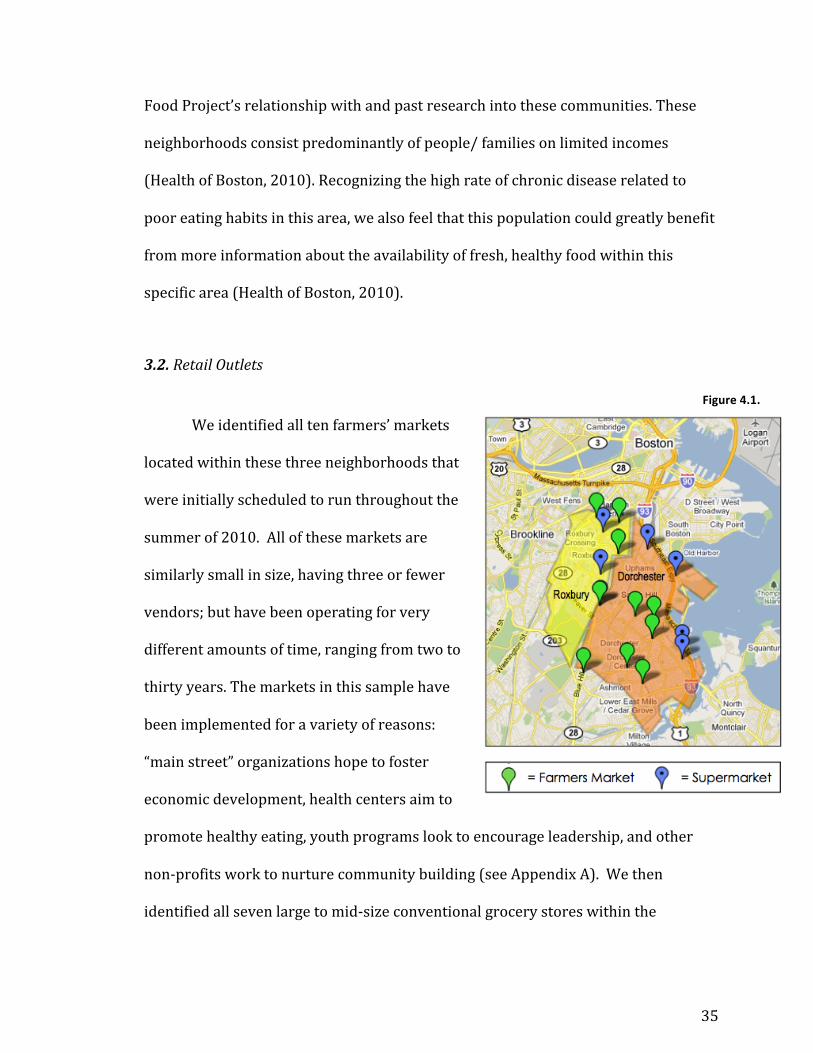
We identified all ten farmers’ markets
located within these three neighborhoods that
were initially scheduled to run throughout the
summer of 2010. All of these markets are
similarly small in size, having three or fewer
vendors; but have been operating for very
different amounts of time, ranging from two to
thirty years. The markets in this sample have
been implemented for a variety of reasons:
“main street” organizations hope to foster
economic development, health centers aim to
promote healthy eating, youth programs look to encourage leadership, and other
non-‐profits work to nurture community building (see Appendix A). We then
identified all seven large to mid-‐size conventional grocery stores within the
Figure 4.1.
36
geographic area based on conversations with residents regarding the most
frequented stores. All of the retail outlets accept EBT/ SNAP and WIC coupons; all of
the farmers’ markets also accept FMNP coupons, senior coupons (SFMNP), and
participate in the Boston’s Bounty Bucks double voucher program (which provides a
50% discount for EBT card users up to $20).
3.3. Time Periods
Using the anticipated starting and ending dates for the
markets, we identified a sixteen-‐week period from July 5 to October
24 during which all of the farmers’ markets would be open for the
2010 season. To account for predicted fluctuation in produce price
and availability throughout the market season, this period was
divided into eight separate 14-‐day periods. Data for each location
was collected exactly one time within the same time period, and is
assumed to be representative of average values during those 14
days.
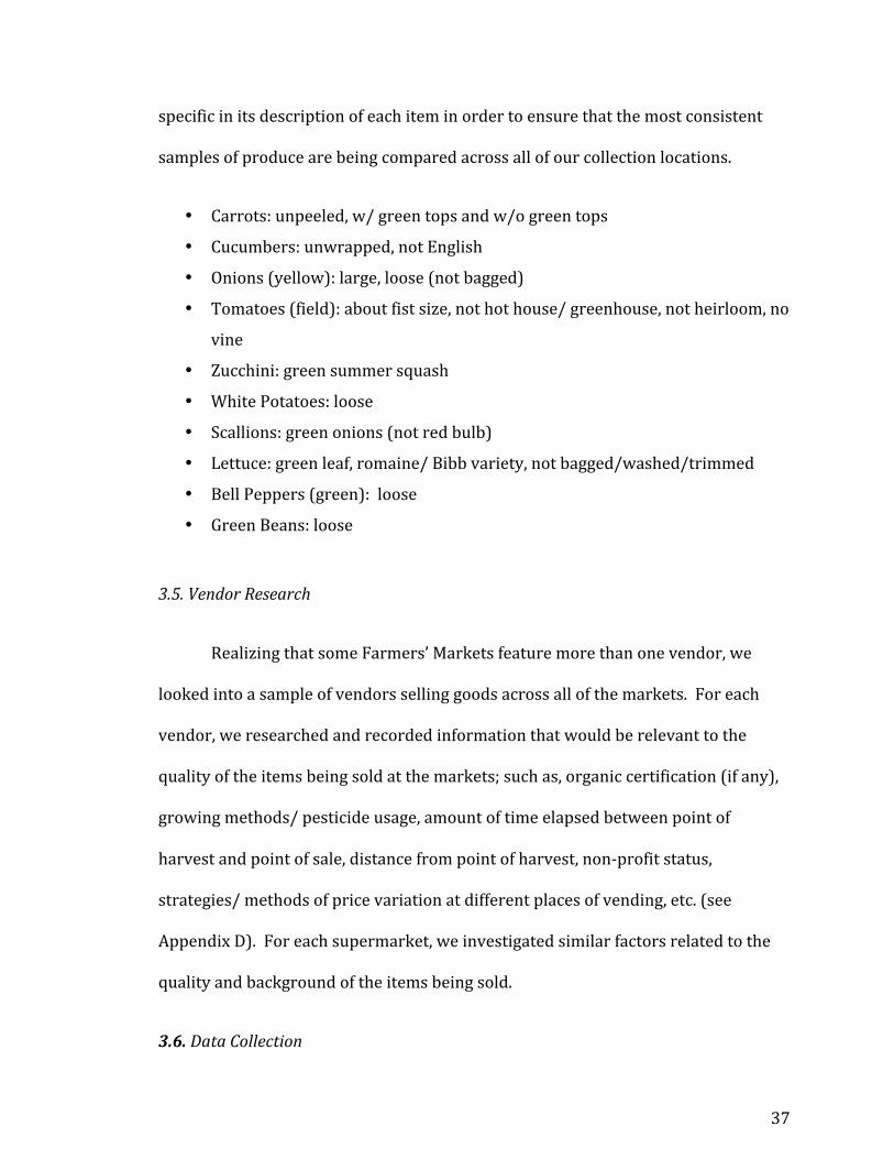
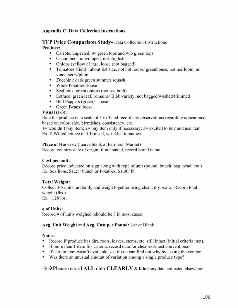
3.4. Produce Types
The study identified ten types of produce that represented common “staple”
food items for the local population. This list also reflects a selection of items that we
found, through research and inquiry with vendors in the study, would be most
readily available at markets throughout the course of the season. Further, we chose
items for which specific type/ growing conditions are not as important (compared
to the price differences among varieties of apples, for instance). This list is very
Figure 4.2.
37
specific in its description of each item in order to ensure that the most consistent
samples of produce are being compared across all of our collection locations.
• Carrots: unpeeled, w/ green tops and w/o green tops
• Cucumbers: unwrapped, not English
• Onions (yellow): large, loose (not bagged)
• Tomatoes (field): about fist size, not hot house/ greenhouse, not heirloom, no
vine
• Zucchini: green summer squash
• White Potatoes: loose
• Scallions: green onions (not red bulb)
• Lettuce: green leaf, romaine/ Bibb variety, not bagged/washed/trimmed
• Bell Peppers (green): loose
• Green Beans: loose
3.5. Vendor Research
Realizing that some Farmers’ Markets feature more than one vendor, we
looked into a sample of vendors selling goods across all of the markets. For each
vendor, we researched and recorded information that would be relevant to the
quality of the items being sold at the markets; such as, organic certification (if any),
growing methods/ pesticide usage, amount of time elapsed between point of
harvest and point of sale, distance from point of harvest, non-‐profit status,
strategies/ methods of price variation at different places of vending, etc. (see
Appendix D). For each supermarket, we investigated similar factors related to the
quality and background of the items being sold.
3.6. Data Collection
38
The study consists of first person observations and data collection (see
Appendix B) at all farmers’ markets and supermarkets throughout the course of the
2010 summer market season, defined as July 5 to October 24. All observations per
time period were taken within the same 14-‐day span, each period beginning on a
Tuesday and ending on a Monday. Based on farmer and vendor interviews, we
assumed that farmers’ market prices were consistent throughout each respective
day the market was operating and did not fluctuate from market opening to closing
on the date observations were made2. All individuals who collected data at any
point throughout the survey went through a training workshop prior to collection in
order to ensure consistency of data collection at all times and locations (see
Appendix C). All vendors were notified of our study prior to collection in order to
enable cooperation and support.
For each item at a location, the price per pound was recorded as labeled;
however, many items were sold in a unit other than pounds (per head, per bunch,
per bag, per each). In this instance, a random sample of three units was weighed on
a scale to obtain an average weight for that item at that location. The price per unit
was then converted to a price per pound based on the average weight of the item in
each random sample. An average price per pound was collected for each vendor
independently and later combined into an overall mean price per pound for each
market. At each farmers’ market, prices from all vendors were observed to the best
of our ability but may have varied according to availability of item, cooperation of
2 Several vendors frequently dropped prices at the end of the market to move produce, but we did not have the capacity to capture time discrepancies in price for each market and hope staggered collection times account for some of this potential discount opportunity.
39
vendor, and precision/accuracy of scale(s) used. If an item was not available for any
reason, its price was not recorded, even if it had been available earlier in the market.
At each conventional market, the same process was implemented with
regard to non-‐pound units. In the case that more than one option of a produce type
is on display, we recorded data for the smallest, most conventional (i.e. non-‐organic)
unit sold. This means that if loose field tomatoes were available in both organic and
non-‐organic varieties, we would record data for the non-‐organic variety; or, if
carrots without greens were available only in 2 lb., 5 lb., or 10 lb. bags, we recorded
data for the 2 lb. bag. While aware that several conventional supermarkets have
volume or “loyalty card” discounts available, we did not take these into account
because such discounts were not consistent with farmers markets’ pricing schemes
and because low-‐income households are often cash-‐constrained and not able to take
advantage of such bulk purchasing.
Data collection also included recording an indicator of visual quality.
Collectors commented on and ranked the overall visual quality of the produce type
on display using a scale of 1 to 3 where 1= “wouldn’t buy the item”, 2= buy “item
only if necessary”, and 3= “excited to buy and use item” (see Appendix E for
examples). In some cases, collectors couldn’t decide between whole numbers and
resorted to using 1.5 or 2.5. In order to treat quality consistently, all half-‐number
values (50 total) were rounded toward the mode rating for the same produce item
at the same vendor or supermarket across all time periods.
There were a few occasions when it was found at the last minute that none of
the collection proxies were able to collect the data for a certain location for a time
40
period or there was a miscommunication where a market was missed entirely. In
these cases we conducted phone interviews with each vendor immediately upon
realizing the mistake in order to collect their availability and prices from the most
recent missed market. For example, the Ashmont farmers’ market was rained out
on the second Friday of collection period 3 and the data had not been collected on
the first Friday, so we acquired information about what was available at the first
Friday’s markets and what the prices were. Since we could not be present to weigh
items sold in units other than pounds, we interpolated unit weight by averaging
average unit weights for one unit of that item across all time periods and used the
period of interest’s unit price to calculate a standardized price per pound value. So
to approximate the price per pound of carrots sold for $2.50 per bunch by Spring
Brook Farm (Vendor) at the Ashmont Farmers’ Market during time period 3, we
calculated the average unit weight of a bunch across all time periods that it was
available [(.75+1.33+. 93)/3= 1.00 lb.], then followed the standardizing calculation
used for all data [$2.50/1.00 lb. = $2.50/lb.]. While we initially withheld data for
non pound units when corresponding unit weight was not provided, because of the
number of missing data points overall due to highly varying produce availability
from week to week, we felt it was reasonable to estimate these data points because
we were certain the item was available at the time but it was logistically impossible
to obtain a unit weight. The same averaging process was also done to obtain each
items estimated visual rating. Data for a certain price in a certain time period was
never interpolated for a produce item that was not available during that period, as
41
we recognize availability is an important factor in reviewing produce at both
farmers markets and supermarkets.
4. Statistical Analysis
4.1. Statistical Method
The primary goal of this analysis was to determine the difference, if any,
between price per pound of produce items at farmers’ markets and price per pound
of produce items at supermarkets. We also wanted to determine whether the
difference between price and retail location type could be explained by other
variables, namely produce type, time period, and quality rating. Multiple regression
was used to control for these other variables.
Regression analysis uses one response/dependent variable and one or more
predictor/independent variables to estimate a mathematical model that describes
the direction and strength of the relationship between these variables of interest
(Kleinbaum et al., 1998). Forming a model with various parameters based on a
research question allows for the construction of hypotheses that can be tested to
provide information about a certain parameter’s slope estimate and its significance.
After reviewing all of the collected data, I specified a series of models and
hypotheses for the effects of single and combined variables based around mean
price per pound as the important outcome variable of interest. Statistical analyses
were performed using STATA, version 9.0 (StataCorp, College Station, TX, 2008).
4.2. Defining the Regression Model
42
In defining the regression model, I concentrated on constructing a model
most relevant to the research question of “How does the mean price per pound
(PRICE) change with variation in location type (LOCATION), while produce type
(PRODUCE), time period (TIME), and quality rating (QUALITY) are held constant?”
For this model, the dependent variable throughout the succeeding regression tests
is the standardized mean price per pound [PRICE (Y)] of a fixed amount of a
produce item. All four independent variables of interest are categorical and are
added in succession to assess relative importance and individual trends. To
distinguish between the two options for the non-‐fixed independent variable
LOCATION, the codes 1=Farmers’ Market or “FM” and 0= Supermarket or “SM” were
used. The numbers 0-‐7 correspond to the eight periods of TIME, the numbers 0-‐9
identify the ten unique types of PRODUCE, and the numbers 0-‐2 are used
categorically to denote QUALITY rating along the previously described 1-‐3 scale of
assessment. These variables were then converted into sets of dummy or indicator
variables for each time period, produce, and quality category.
Note that if a nominal variable has k categories, then k-‐1 indicator variables
are assigned to index these categories because the first level of each nominal
variable is indicated by the presence of zeros in all of the hypothetical reference
cells (i.e. there are a total of 8 time periods, but only seven indicator variables are
used because “time1” is actually the indicator variable of time period 2, “time2” is
the indicator variable for time period 3, and so on). The complete population
regression model below represents the full model of price variation between
locations while controlling for fixed effects with each set of indicator variables. As
43
was mentioned earlier, fixed effects are added in succession to provide alternative
angles of analysis. The command “robust” is added to account for the fact that there
may be heteroskedasticity in the error terms.3
The value of β0 represents the intercept and varies according to the equation,
and the reported value of β1 represents the estimated coefficient of variation for the
variable of primary interest, which is the location of the sale.
4.3. Description of Sample
Preliminary descriptive statistics (Table 4.1) relate a helpful outline of the
data before introducing and controlling for other variables. Out of 1760 possible
observations of price (and quality) at both farmers markets and supermarkets at the
outset of this study, a total of 1032 data points were actually recorded. Despite the
initial over-‐representation of possible observations at farmers’ markets due to a
higher number of vendors and collection sites, both location types have fairly equal
representation in the final data set, with 52% from farmers markets and 48% from
3 This will tend to give more conservative estimates of the standard errors (and p-‐values).
A chart of TIME vs. PRICE for each location type without accounting for
produce type or quality rating (Figure 4.4) illustrates how overall mean price at
each location type varies throughout the 8 time periods. An overall decreasing
trend in mean price per pound at farmers’ markets is contrasted with a relatively
constant and ultimately increasing trend at supermarkets. At farmers markets,
there was a 14% initial drop in mean price across time periods 1 and 2, followed by
a slight increase from period 3 to 4, and ending with another large decrease of 19%
over the final four time periods. Supermarkets reported a very constant mean price
from time periods 1 through 7, never deviating more than 0.03 from the mode 1.69,
but saw about a 10% increase during time period 8. Interestingly, the largest
differences in mean price per pound occurred during the very first and last time
periods. In time period one, mean price at farmers’ markets ($2.01) was about 18%
higher than at supermarkets ($1.70); while in time period 8, mean price at
supermarkets ($1.89) was a striking 28% higher than at farmers’ markets ($1.48).
Introduce Produce Type
Graphs of TIME vs. PRICE at each location type for each produce item
separately demonstrates how overall mean price for each type of produce varies by
location over the course of the summer season (see Appendix I). First, cucumbers
at farmers’ markets exhibited a slightly decreased price trend overall (though still
significantly more expensive than at supermarkets), marked by a notable sudden
decrease in mean price/lb. by about $0.40 during time period 6 (9/13-‐9/26). A very
similar pattern was followed by farmers’ market bell peppers, which exhibited a
momentary $0.60 decrease in mean price/lb. during the same time period 6 (see
57
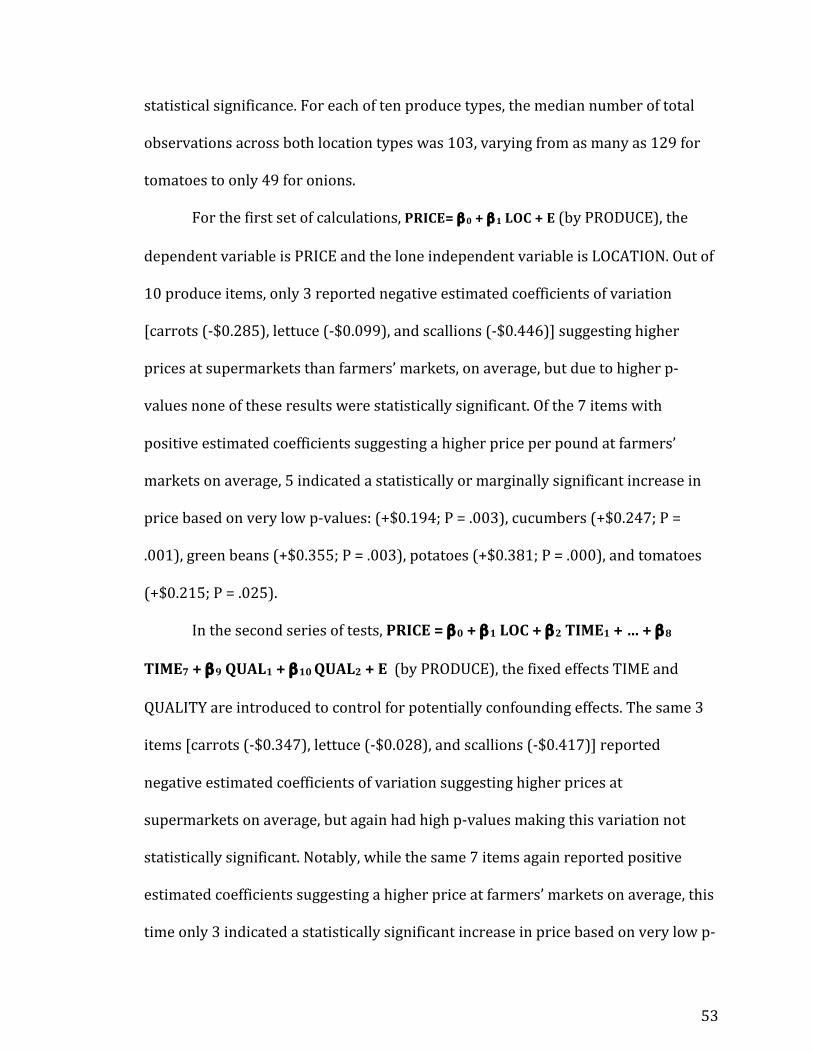
figure 4.5). Interestingly, zucchini showed an opposite pattern, with an overall
increasing trend punctuated by a momentary $0.50 increase in mean price/lb.
during week 6. The mean price/lb. of carrots dropped rapidly by $0.50 during time
period 4 (8/16 -‐8/29), recovered, then dropped rapidly again by nearly $1.00
between periods 6 and 8 (9/13-‐ 10/24). The price/lb. of scallions spiked by $1.50
during time period 4 (8/16-‐8-‐29), and the price/lb. of lettuce spiked by about $1.25
during time period 5 (8/30-‐9/12) (see figure 4.6). Onions demonstrated a rapid
decline of about $1.40 from the start of the study until time period 3 (7/5-‐8/15),
and then remained relatively stable at the decreased price/lb (around $1.00).
Potatoes acted similarly, showing a decrease of nearly $1.00 (from $2.00) between
time periods 1 and 3 (7/5-‐8/15), and then staying between $1.00 and $1.50 for the
remainder of the market season. Interestingly, the mean price/lb. of green beans
increased at farmers’ markets and decreased at supermarkets during the same time
periods (4-‐7) by about the same margin.
5. Discussion of Results 5.1. Summary
These results offer some support to the widespread consumer perception that
produce costs more at farmers’ markets than at supermarkets in the underserved
Boston neighborhoods of Roxbury and Dorchester, but the difference is not very
large. I found that when time period, quality rating, and produce type were held
constant, the mean price per pound of produce at area farmers’ markets was a
marginally significant 8.6 cents greater than at supermarkets, on average. With the
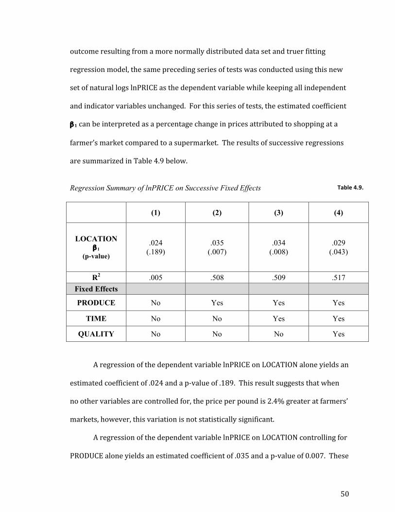
dependent variable lnPRICE, the log of price, the results suggest a significant 2.9%
58
increase in price per pound on produce at farmers’ markets compared to
supermarkets. In addition, I found that bell peppers, cucumbers, and potatoes cost
significantly more per pound at farmers’ markets when the effects of time and
quality were controlled for. A plot of time period vs. mean price per pound by
location showed that prices at farmers markets decreased markedly throughout the
sixteen-‐week season, while supermarket prices remained nearly constant before a
noticeable increase during the final time period. As anticipated, overall quality
rating was significantly greater at farmers’ markets than at supermarkets. The
robustness of the statistical results on overall price differences was also confirmed
using a natural log transformation of price.
5.2. Magnitude of Price Differences
The statistically significant 2.9% increase in mean price per pound of
vegetables at farmers’ markets (from the log of price model) indicates that farmers’
market produce is more expensive, on average, than produce purchased from
traditional grocery outlets. But what is the practical significance of this variation to
the consumer? Several researchers have found that fruit and vegetable
consumption is lower when fruit and vegetable prices are higher (Powell and Bao,
2009), yet do these results imply a noteworthy obstacle to produce consumption via
a farmers market in certain Boston neighborhoods? It may be difficult to have a
concrete sense for how much “value” or weight about 3% carries, so I will translate
this amount into an estimated total cost increase if a consumer purchased produce
only at a farmers’ market throughout the summer season. The Economic Research
Service of the USDA recently published a report of fruit and vegetable prices
59
declaring that an adult on a 2,000-‐calorie diet could satisfy recommendations for
fruit and vegetable consumption (amounts and variety) in the 2010 Dietary
Guidelines for Americans at an average of $2 to $2.50 per day (Stewart et al., 2008).
By using the mean of this range, $2.25, an increase by 3% would increase daily cost
of consuming the recommended fruit and vegetable amount by about 7-‐cents to
$2.32. Over the course of the 16-‐week/112 day summer market season used in this
study, purchasing the recommended daily amount of produce would increase from
$252.00 to $259.84-‐ nearly $8.00. Though more weighty for a price-‐sensitive
shopper, I consider an additional $8 over the course of nearly four months to be a
relatively minimal cost to the average shopper’s wallet. Of course, the ERS
estimation does not provide an entirely precise basis for analysis given that it was
derived from national data (Boston has a history of food prices higher than the
national average), that most Americans do not consume recommended amounts,
and that it also includes fruits, which were not considered in this study. Even so,
this sort of extrapolation provides an approximate number that may be helpful in
conveying a more realistic message of actual cost differences to residents of
Dorchester and Roxbury and to policymakers responsible for incentivizing the
purchasing/consumption of fresh produce.
In its measurement of price per pound of produce, a few notable limitations
are encountered by this study’s methodology. First, data was recorded based on
standardized price per pound of produce as it would be presented to a customer at a
retail outlet and was not adjusted to represent an edible equivalent (stems, skins,
greens, and other non-‐edible parts removed). The USDA’s ERS examined the
60
importance of such an adjustment and found that retail prices appeared to be a poor
indicator of prices per edible cup equivalent, though great variation based on
produce type existed. Next, this study did not differentiate between produce sold on
a random weight basis ($1.29 per pound for loose tomatoes) and produce sold in
prepackaged containers bearing retailer’/manufacturer’s name or produce sold on a
“count basis” ($2.00 per 2 lb. bag of carrots or $1.50 per head of lettuce). Overall,
the USDA’s ERS suggested that a distinction in produce marketing form was not an
important factor in price, but often prepackaged containers or bags offered bulk
discounts that are important to mention. When collecting data, this study recorded
prices for the smallest amount of the conventional type of produce and did not
include prices for bulk packages (5 lb. bag of potatoes) because it was assumed that
customers on a limited budget may not be able to take advantage of volume
discounts, and also because farmers’ markets rarely offer such discounts. This
decision is backed by Kunreuther et al. (1973), who argued that the poor are
disadvantaged because they are unable to participate in the purchase of economy-‐
sized packaged goods due to the limits of available grocery money and storage
space. While this is a legitimate assumption, many shoppers are able to take
advantage of significant bulk discounts at supermarkets that are not as readily
available at farmers’ markets; for example, Shaw’s loose onions were sold for
$1.79/lb. compared with a 2 lb. package of onions for $0.92/lb (about a 50%
discount), and Tropical Foods sold loose potatoes for $0.79/lb. compared with a 5
lb. bag for $0.34/lb (nearly a 60% discount).
61
Lastly, special discount offers were available at both location types but were
not factored into price analysis. Supermarkets offered some sort of “frequent
shopper” discount almost weekly where shoppers with say, a “Stop and Shop Card”
could benefit from special price cuts like zucchini for $0.50/lb. (regular price =
$1.49) or green beans for $0.20/lb. (regular price = $1.69). Farmers’ market
shoppers receiving SNAP assistance frequently benefited from utilizing the city-‐
wide incentive program “Boston’s Bounty Bucks” to save 50% on purchases up to
$20.00. Interestingly, when shoppers took full advantage of the Bounty Bucks
program and selected $20.00 worth of produce, they were able to save $10.00 at a
farmers’ market in just one trip-‐ the same amount that my earlier extrapolation
suggested as the total additional cost at farmers’ markets over the course of the
summer. This comparison quite clearly implies that, for low-‐income residents of
Boston who receive federal SNAP assistance, shopping at a farmers’ market may in
fact be an extremely economical way to maximize monthly benefits while reaping
the greater nutritional advantages of fresh produce.
5.3. Availability
One major drawback of farmers’ markets highlighted by the data was the
relative frequency of unavailable items. Only 45% of the initially assigned data
points were available at farmers markets, compared with 88% at supermarkets.
This result is most likely influenced by heightened time and climate sensitivity at
farmers’ markets. Vendors are limited by what they can transport to the market
from the farm, usually only assign one vendor/vehicle for small markets in these
neighborhoods, and in many cases supply quantities reflective of low demand.
62
Consequently for collectors, the later data collection took place, the more likely it
was that an item was sold out and therefore excluded from the final data set.
Enhancing this obstacle is the fact that the markets included in this study were
usually scheduled to open only one day a week (two markets opened two times a
week) for a few hours, further limiting collectors as to when data could be recorded.
Also, it must be noted that data only reflects the availability of the ten chosen
produce items rather than overall produce stock, thus in most cases it does not
adequately express the wide variety and plentiful supply of other produce items at
farmers’ markets. For example, most vendors had some sort of green leafy produce
available (spinach, calaloo, arugula), but since these items are subject to vast price
variation at supermarkets and less certain availability at farmers’ markets, they
were not included and their availability not reflected. On many occasions when a
certain item was not recorded and thus deemed unavailable, closely similar items
were in fact available at farmers’ markets (plum or cherry tomatoes, red potatoes,
“salad mix”), but were not included because they did not fit the specific criteria for
comparison. Still, the limited supply and unpredictable availability of farmers’
markets are not only obstacles to data collection and analysis, but also more
significantly are a major hindrance to their utilization and popularity among
residents and shoppers.
While this expected pattern of decreasing availability due to limited supply at
farmers’ markets is clearly a disadvantage, it is further and perhaps unfairly
exaggerated by comparing it to the endless supply of produce available to larger
distributors and supermarkets. Unlike supermarkets that rely on a continental
63
network of greenhouses, massive farm operations, and refrigerated storehouses,
farmers’ markets are directly sensitive to the day-‐to-‐day growing conditions of
specific items and can only sell what is locally available for harvest. For a growing
number of Americans, this closeness with the farm and acceptance of nature’s
unpredictability is appreciated and even favored over the dependable stock of
supermarkets (Whitacre, 2009), but I speculate that such an attitude is not a reality
for residents in low-‐income neighborhoods. Though contemporary popular and
academic culture may suggest that the enormous network of processed agricultural
commodity crops is negatively affecting our health and environment, its ability to
create a consistent, reliable supply of fresh produce is highly valuable to the lower-‐
income consumer. The truth is that low-‐income shoppers in particular tend to make
fewer monthly trips to buy groceries due to transportation, federal support, and
proximity constraints (Whitacre, 2009); therefore, a larger distributor maximizes
options for those not likely or capable of making multiple trips to buy food.
On the other hand, however, the existence of these ten farmers’ markets in the
middle of dense neighborhoods puts fresh produce closer within the reach of
households that need it most. Larsen and Gilliland (2008) showed that for residents
of low-‐income urban communities that purchase food based on proximity due to
transportation constraints, the increased access to healthy foods provided by a
farmers’ market would likely improve some household diets. Regardless of how
small any market’s selection is, the quality, freshness, and nutrition of the produce
far surpasses that of the produce and food options at other neighborhood bodegas
and corner stores that supplement trips to larger, more distant supermarkets.
64
5.4. Quality
The incorporation of a quality rating into this study was meant to assess the
common hypothesis that farmers’ market produce, while more expensive, is
undoubtedly of better quality. Results support this hypothesis, showing that
farmers’ markets received a significantly greater proportion of highest quality
ratings than did supermarkets. While this difference in quality is certainly justified
by data and first-‐hand accounts, it is necessary to note the limitations inherent in
measuring produce quality. As quality is a subjective assessment prone to all sorts
of individual preferences, studies involving produce/foodstuffs often choose to
disregard it altogether for fear of jeopardizing the objective validity of their
research. I feel that quality is an extremely important aspect of a consumer’s
decision-‐making process and it must not be dismissed or ignored but rather handled
with caution. In designing a system for measuring quality, this study aimed to
minimize subjective influences by using a limited range of values (1-‐3) and training
all collectors using reference examples for each rating. Since most people rely on it
when selecting items to purchase, visual rating is a realistic and useful form of
quality assessment that plays a particularly strong role in the discussion on food
access. It is worthwhile to acknowledge that the measure of visual quality rating
used in this study is not necessarily a parallel indicator of taste, which has been
shown repeatedly to play the most influential role in fruit and vegetable
consumption decisions (Glanz and Goldberg, 1998; Reicks et al., 1994; Treiman et
al., 1996). However, in her discussion on food-‐purchasing decisions, Cummins
(2010) remarked that perceived quality of produce, (i.e. what a shopper infers about
65
taste, freshness, and nutrition based on visual presentation) is a very important
factor, and likely acts as a mediating variable in the decision to buy fresh produce.
Additionally, a similar survey by French (2002) concluded that individuals of lower
socioeconomic status -‐like those central to this study-‐ might place greater
importance on this perceived quality than on actual taste, freshness, or nutrition.
These references assert the importance of first impressions of produce quality in the
overall perception of value and verify the decision to incorporate perceived quality
rating in this study.
Knowing that 1) lower-‐income families purchase/consume less fresh produce
than higher-‐income families and 2) lower-‐income families have reduced
accessibility to good quality fresh fruits and vegetables, these results indicate that
farmers’ markets are introducing produce items of higher perceived visual quality
into surrounding communities. Traditionally, local corner stores in Dorchester and
Roxbury tend to stock produce from Chelsea Produce Terminal, often just to fulfill
new WIC requirements on minimum produce offerings; thus, whatever produce
they sell is likely of low quality in an effort to keep prices as low as possible
(Whitacre, 2009). The likely effect of this pattern is recounted by Hendrickson et al.
(2006) found that residents in underserved Minneapolis communities felt that, even
if they had the money to spend on fresh produce, the quality of produce in their area
was so poor it would not be worth it. By making higher quality produce more
available, lower-‐income consumers are more likely to purchase fruits and
vegetables previously deemed undesirable, enjoy eating them, and continue to
include produce in their diet.
66
Though important inferences can be drawn from this study’s results, there are
countless ways in which the assessment of quality can be enhanced in future
research. Ideally, more intensive training would be required to provide all
collectors with uniform examples of each produce item at each rating level.
Collectors would also benefit from the use of a visual/pictorial reference guide when
making assessments in the field. Finally, a systematic series of blind taste tests and
shelf-‐life assessments would account for the fact that taste and perishibility are two
other very important qualitative factors in deciding overall value and whether or
not to purchase an item again.
Growing and Harvesting Methods
When discussing quality, it is also important to mention the variations in
growing methods used by supermarket producers and local farmers’ market
vendors. First, almost all supermarket produce included in this study was not
specified as “organic” or “organically grown”, and based on information provided by
produce managers at all supermarkets, is assumed to be grown according to
conventional large-‐scale agricultural methods including the active use of pesticides.
The one major exception to this assumption is the case of Stop and Shop’s scallions,
which were heavily marketed as “organic” at all stores via the name “Nature’s
Promise”. Research uncovered that Stop and Shop is able to mass-‐produce organic
scallions in Mexico for an inexpensive cost and may use them as a “loss leader” by
presenting an organic product at an unusually low price (Danielle Andrews,
personal communication, summer 2010).
67
As for the fourteen vendors at the ten farmers’ markets in Dorchester and
Roxbury, two vendors (Serving Ourselves and Langwater Farms) were certified
organic and the thirteen others all reported using organic, sustainable farming
practices but were not officially certified. In many cases these farms were practicing
“Integrated Pest Management” (IPM), which involves very minimal pesticide usage
and is required for at least a year prior to becoming certified organic. Urban farms
like The Food Project, Revision House, and Village at Work used almost entirely
organic methods, but could never become certified organic because they lie within
50 feet of the road and are too close to neighbors who may be using pesticides
(Cammy Watts, personal communication, summer 2010). The major barrier to
organic certification, however, is the enormous expense to the farmer. Following
the initial costs of transforming the agricultural structure of a farm and becoming
certified, additional costs are constantly required to renew the certification,
maintain high standards of organic practices, and change marketing strategies
accordingly. These expenses are the reason that certified organic produce almost
always costs more at any retail outlet and also create a financial barrier to the
consumption of organic produce by low-‐income shoppers. While the nutritional
benefits of organic produce are still being debated, there is some evidence to
suggest that organic produce contains higher levels of nutrients and tastes better
than produce grown using pesticides; plus, buying organic undoubtedly supports
the efforts of farmers who are aiming to improve the ecological health of the land
that they farm on (Reganold, 2001). Therefore, the fact that customers are able to
buy organically grown produce at farmers’ markets in Dorchester and Roxbury
68
without incurring the transfer of additional costs due to organic certification means
that shoppers are likely getting a higher quality item for a lower price than would be
marketed at a supermarket. While most low-‐income consumers would not usually
pay more for an organic item, there is potential for them to appreciate the idea of
being able to purchase organically grown fruits and vegetables to feed their
households, leading to an overall increased motivation to shop at and consume
produce from farmers’ markets4.
5.5. Seasonality
When proposing her dissertation research project on farmers’ market produce
in North Carolina, Natalie Valpiani, a Masters candidate at the Tufts Friedman
School of Nutrition Science and Policy noted that the widely held idea that produce
prices change according to season is a concept that many intuitively take for
granted, yet there is little data supporting such conclusions (personal
communication, July 2010). In particular, seasonal changes in price would likely be
attributed to certain produce types in certain regions and climates. The inclusion
and controlling of time effect in this study was meant to better gauge what impact, if
any, seasonality had on the prices of ten produce items over the course of a New
England summer.
4 Note: although this secondary qualitative factor was not anticipated to be a selling point to
the price-sensitive shopper featured in this study, the behavior during the summer of 2010 suggested otherwise: a report on the use of Boston Bounty Bucks found that, at Copley Square-one of Boston’s most popular and expensive markets, SNAP redemption amounts were second highest at a certified organic vendor, Atlas Farms (Cammy Watts, personal communication, March 29, 2011). This surprising statistic might indicate that when using “free money” from the Bounty Bucks program, even lower-income shoppers prefer purchasing organically grown produce.
69
Due to the temperate climate of the Northeast, most agricultural crops can
only be produced outside greenhouses during the months between late spring and
early fall. As a result, locally grown produce is subject to strong seasonal price
fluctuation during these months based on the highs and lows of each produce type’s
unique growing pattern. Generally, such seasonal price changes at the farm level
have diminished impact on retail prices at larger distributors like supermarkets due
to many more overhead costs such as advertising, packaging, and transportation
(Fisher, M., 2009). In contrast, selling directly to the consumer enables farmers to
avoid these overhead costs, allowing them more flexibility to adjust prices based on
surplus or scarcity in the supply of any individual crop. This means that the
consumer has the ability to take advantage of periodic, often significant price
reductions at farmers’ markets resulting from an overabundance of a particular
crop at the height of its growing season. By recognizing and accounting for such
potentially significant price fluctuation over the course of the market season, this
study makes improvements over previous research that ignored the effects of time
entirely and therefore may have produced misleading, skewed results (Pirog &
McCann, 2009).
The overall results of this study show greater fluctuation and a general
decreasing price pattern at farmers’ markets, while supermarket prices kept
extremely stable until a marked increase during time period 8 (see figure 4.4). This
likely suggests that supermarkets changed their producers from outdoor growers
during the summer months to pricier greenhouse growers once the weather began
to turn cold. One pattern that shows quite apparently on these individual time plots
70
is that of the consistency of price/lb. at supermarkets versus greater volatility in
price at farmers’ markets.
Plotting time period against mean price/lb by location type for each produce
item separately reveals more information as to how changes in specific crop
availability may have influenced overall price trends (see appendix I). For example,
cucumbers and bell peppers were consistently more expensive at farmers’ markets,
but both showed a notable drop in price below that of supermarkets during time
period 6, possibly indicating a surplus harvest. Likewise, the mean price per pound
values of scallions and lettuce were somewhat even at both locations up until
periods 5 and 6, respectively, when farmers’ markets became much less expensive
through the end of the season. Importantly, prices for all produce items except
scallions were higher at farmers’ markets during time period 1, and many continued
Time Period
Time Period Time Period
Time Period
Figure 4.5. Figure 4.6.
71
to be noticeably higher until period 2. This may be due to vendors’ starting prices
high and then adjusting to consumer response or because it was still early in the
season and farmers had smaller harvest. Regardless, initial impressions of a
farmers’ market as having higher prices early in the season have the potential to
deter shoppers from returning in the future when prices are lower.
5.6. Produce Type
With numerous types of produce available for purchase at most conventional
grocery outlets, the ten specific types chosen for this study reflect deliberate
planning. One thing that a majority of studies on fruit and vegetable consumption
consider when selecting which types to investigate is the National Health and
Nutrition Examination Survey (NHANES) data ranking consumption rates of the
most popular produce items. This national reference was not considered when
selecting produce types for this study, meaning that our results do not necessarily
convey information about the most popular vegetables and may therefore lack
relevance to consumer preferences. This should not be considered a serious
limitation for several reasons. First, national averages do not necessarily reflect the
preferences of ethnic minorities and/or low-‐income consumers such as those living
in Dorchester and Roxbury. Aware of farmers’ markets’ less predictable stock of
produce, the selection process did not intentionally overlook this nationally
referenced data but instead decided to choose based on farmer and farmers’ market
manager interviews regarding which produce types would be most frequently
available in order to maximize realized data collection.
72
One trend noted throughout the season at farmers’ markets was the presence
of vegetables that looked different or were of a slightly differently variation than the
conventional type of produce consumers have come to expect in supermarkets.
Some items may look slightly different or vary more in size/shape/appearance than
what you would expect to find at a supermarket because the produce at farmers’
market is not grown according to mass-‐agricultural specifications for conformity.
Similarly, produce at a farmers’ market often comes with a bit more dirt residue
than you’d expect to find at a supermarket because massive cleaning machines
aren’t feasible for farmers and vendors place lesser emphasis on the presentation of
a clean, glistening product than do supermarkets. These less-‐perfect characteristics
may be appreciated as reminders or evidence of the straight-‐from-‐the-‐ground
freshness and local origin of farmers’ market produce, but they could also deter
consumers who aren’t used to such variation in appearance and are hesitant to try
something new, or who interpret more dirt as more time and effort needed to clean
and prepare produce.
Although relatively limited compared to the selection of more traditional
fruits and vegetables at a supermarket, farmers’ markets frequently seemed to serve
an important function in enabling ethnic and cultural cooking traditions that play an
important role in food choice and meal preparation (Fisher, A., 1999). It was
apparent that shoppers of different ethnic backgrounds appreciated and purchased
certain non-‐mainstream produce types with excitement while expressing their
frustration over the absences of these culturally important items in conventional
markets or corner stores (calaloo, green tomatoes, collards). The ability for
73
farmers’ market vendors to tap into ethnic appetites not satisfied by supermarkets
is an important aspect of their ability to encourage produce consumption.
Overall, it is likely that farmer’s markets tend to offer a significantly better variety
and quality of produce items than what is currently available at nearby corner
stores in Dorchester and Roxbury. Improved selection could enhance the
purchasing experience and therefore increase the likelihood of produce
consumption.
5.7. Contributions of Methodology
This study has proved successful in accomplishing one of its major
objectives-‐ to pilot a methodology that could be used by other organizations and
policy surveyors to assess the affordability of farmers’ markets within specific
neighborhoods rather than larger, diverse metropolitan areas. Since it is yet to be
determined if national findings on socioeconomic and geographic factors relating to
food access can be broadly applied to smaller areas with similar demographics
(Whitacre, 2009), applying this methodology to a geographically, demographically,
and socioeconomically well-‐defined area will also add to the proposed “Healthy
Incentives Program” (HIP, Farm Bill 2008) research into national farmers’ market
programs by bringing attention to the importance of investigating food access issues
at a more specific community-‐level. Both farmers’ markets and supermarkets are
influenced by the respective needs of their surrounding populations. While
supermarkets have been found to be more expensive in the inner city than in
suburban areas (Ashman, 1999), farmers’ markets are particularly sensitive to the
environment in which they are located and exhibit tremendous diversity in
74
structure, size, composition, product, popularity, and purpose (Fisher, A., 1999). By
emphasizing unique characteristics of the health and diet-‐related environment in
the most local context, this study is able to examine distinct influences on
purchasing and consumption patterns that pertain directly to certain
neighborhoods.
Another significant contribution made by this study is its avoidance of
defining a healthy food-‐deficient area based on the uncertain definition of a “food
desert” or by distance to a supermarket. Nearly all of the literature on racial,
socioeconomic and geographic disparities in food access or food consumption
trends mentions access to supermarkets as an important factor when diagnosing
obstacles to healthy food access (Walker, 2010), yet Dorchester and Roxbury, like
many other urban areas, are not “food deserts” and most neighborhoods fall within
reasonable distance of at least one of the seven supermarkets in this study. These
types of neighborhoods still have needs in terms of access to and education about
healthy food and have complex socioeconomic and perceptual issues related to food
consumption that go beyond the proximity of supermarkets. Realizing that a
household’s proximity to a supermarket is not something that can easily be changed,
especially in dense inner city areas, this study explores the current status of
farmers’ markets as alternatives to supermarkets in economically disadvantaged
neighborhoods.
75
Section 3
Current and Future Implications: The Viability of Farmers’ Markets
in Underserved Boston Communities
While clarification of relative produce price and quality at farmers’ markets
and supermarkets provides an opportunity to encourage the purchase of local fruits
and vegetables in low-‐income neighborhoods, there are many other opportunities to
consider when thinking about the long-‐term potential for farmers’ markets to
positively affect diet-‐related health in underserved communities. Crucial to
understanding the overall value of farmers’ markets is a review of the individual and
community gains they make available. Equally important is a detailed account of the
unique challenges confronted by small farmers’ markets in low-‐income areas.
Drawing from first-‐hand experience and several months of involvement, I comment
on the benefits and barriers facing small farmers’ markets in communities like
Dorchester and Roxbury before proposing a few goals aimed at enhancing their
viability into the future.
1. Benefits of Farmers’ Markets
The potential benefits to be had from the presence of farmers’ markets in
underserved, low-‐income neighborhoods of Boston are numerous. First, farmers’
markets make healthy, fresh food more available to communities in terms of
proximity and convenience. Due to limited transportation and free time due to busy
work schedules, low-‐income households are less likely to travel the distance to a
76
supermarket outside of their neighborhood’s small corner stores, therefore
sacrificing cost and quality for convenience (Walker, 2010). But because the
farmers’ markets in this study are so small and feature only 1-‐3 vendors, they can be
located at closer intervals than larger scale markets and are very flexible with
regard to finding a host location. This means that, for the transportation
constrained low-‐income consumer who values proximity, outlets selling fresh,
higher quality fruits and vegetables are more conveniently available and more likely
to be considered an option when deciding where to purchase food.
Next, because credits can only be redeemed at participating farmers’ markets
(though most Boston markets now participate), the introduction of FMNP/SFMNP
and Boston Bounty Bucks make new money saving opportunities available to SNAP
users while enticing them to buy more fruits and vegetables. Since recipients of
FMNP/SFMNP must use their “free money” at farmers’ markets, the programs
essentially force them to enter a produce-‐purchasing environment that many would
not have chosen otherwise. Through this incentive program users are exposed to
different stimuli and expectations that could potentially change their previous
associations to buying produce for the better. This potential to attract new
consumers is demonstrated by McCormack et al. (2010), whose survey of SFMNP
recipients at farmers’ markets found that 68% of respondents had never shopped at
a farmers’ market before. More importantly, a majority of shoppers in the survey
found the produce quality to be much better or better than at supermarkets, and
38% of those who used SFMNP coupons continued to shop at a farmers’ market in
77
the future, indicating that many new shoppers were impressed and compelled to
return to this new environment.
Not only do farmers’ markets offer a convenient way to obtain healthy food
and an outlet for the redemption of subsidy and coupon credits, but they also do
these things in a unique environment that could change the experience of buying
produce for people in these communities. This study supports several others that
found that farmers’ markets offer produce of a higher quality than what is
conventionally available in area supermarkets and corner stores, and access to
improved quality suggests increased rates of consumption because overall value in
terms of cost and benefit to the consumer is greater (Cox et al., 1997).
Improvements in quality can be attributed to factors such as freshness, organic
growing methods, and nutritional value. Freshness: at the time of purchase, it has
usually only been 24-‐48 hours since the locally grown produce has been harvested
from the earth, making it much fresher than what is sold at most conventional
markets (Farmer Dave Dumaresq of Brox Farm, personal communication, June
2010). Grown using organic practices: all of the produce sold at these farmers’
markets was grown using organic methods or IPM (Integrated Pest Management),
meaning it has been exposed to no or minimal pesticides. Nutritional value: all
produce was harvested on farms located within two hours driving time of Boston,
which means it was not subjected long distance travel that has been shown by some
research to substantially deplete nutrients (Schoonover, 2007).
Outside of produce quality, farmers’ markets also offer positive experiential
qualities like social atmosphere, buying directly from a farmer, and supporting local
78
produce. As a public and social space, farmers’ markets facilitate mingling and
sharing of produce preparation tips by diverse community dwellers of all ages and
serve as a vehicle for community discussion and development; one sociologist even
calculated that people have ten times as many conversations at a farmers’ market
than at a supermarket (Halweil, 2002)! Through the direct sale of produce from the
farmer to the shopper, farmers’ markets also seek to connect local producers with
local consumers in a mutually beneficial educational linkage that encourages
continued patronage (Pollan, 2010). Finally, shoppers who patronize farmers’
markets not only ensure themselves of a more healthy food supply for their families,
but also go a long way toward supporting the survival of small scale sustainable
agriculture and the economy of local farmers and producers.
2. Barriers to Farmers Markets
Though the potential for benefits is large, including providing healthy food
access in these underserved communities, farmers’ markets in low-‐income urban
neighborhoods are experiencing substantial economic, administrative, and social
barriers to their success (Briggs et al., 2010). While aggressive efforts to open
farmers’ markets in underserved urban communities have been applauded and
replicated throughout the country, many of these programs are nearing collapse due
to exhausted funds and low rates of farmer retention. Initially opened as pilot
programs, these small markets are more often than not run by non-‐profit
organizations and community health centers that rely entirely on government
funding to absorb operating costs, in turn making them extremely vulnerable to any
change in funds or donations. On top of the many daily and weekly administrative
79
duties of publicity, legal paperwork, and logistical coordination, most farmers’
market managers are strained by the process of having to ceaselessly and single-‐
handedly apply for grants from federal/state programs, private donors, public
foundations, etc. in order to keep the market afloat. And though positive and
important steps forward, the addition of incentive programs like SFMNP and Boston
Bounty Bucks requires additional administrative work such as applications,
training, troubleshooting, and assistance that further burdens the farmers’ market
manager who already faces exceptional challenges.
2.1. Disproportional Operational Fees
The process and costs of registration, renewal, and retail permits present a
major barrier to small markets in low-‐income areas. There are certain fees
demanded of every market, regardless of size, to be paid to the City of Boston
and/or the Inspectional Services Department (ISD), and for non-‐profit markets that
pay to operate without earning profit, even minimal fees are a financial stressor.
For example, in Boston, there is a fee of $50 for the “Use of Premises” permit to
operate a farmers’ market even on private property. The process of obtaining this
permit involves compiling paperwork locating a certified plot plan for the property
(no easy task in some cases), and making several visits to the ISD office, which
multiple farmers’ market managers have found daunting (Cathy Wirth, personal
communication, summer 2010). Next, farmer’s market managers usually charge a
“market fee” to each farmer who wants to sell at their market in order to raise funds
for basic operating costs. For the markets in Dorchester and Roxbury, charging
farmers to come to a market is not realistic when farmers are already dropping
80
prices and dealing with low sales volume. Also, ISD requires that vendors selling
bread, granolas, or foods other than fruits and vegetables pay a $100 fee for each
market they sell at. Some market managers see breads and non-‐produce items as
ways to draw people to farmers’ markets, but this cost is prohibitive for vendors
coming to markets in low-‐income areas and discourages farmers from selling
popular non-‐produce items that could really boost attendance (Cammy Watts,
personally communication, summer 2010).
2.2. Restrictions on Educational Activities
A farmers’ market serves as an ideal vehicle for education about the health
effects of produce and can provide resources to help shoppers use produce in new,
simple ways. Demonstrations and free samples are some of the most popular
educational activities at farmers’ markets and both add to the atmosphere of the
market and attract shoppers. Unfortunately, Boston has some of the most
restrictive regulations around sampling at farmers’ markets of any city in the state.
Market managers and farmers’ market advocacy groups have been struggling with
these restrictions for years, and have brought their concerns to organizations
including the Mayor’s Food Council and the MA Department of Agriculture. (Cathy
Wirth, March 28, 2011). Efforts to work within the limits of the existing regulations
have been challenging. Last summer a group of nutritionists at UMASS Extension
wanted to conduct small food preparation demonstrations with samples at each
market to show shoppers simple methods for using available produce. Tremendous
effort and compromise was required to come to an agreement with ISD regarding
the health precautions that would be required, and it was decided that the group
81
must prepare the samples in a certified off-‐site kitchen and then offer them in
sealed, refrigerated containers (UMASS representative, personal communication,
July 2010). During the first few weeks of the market season the samples, along with
piles of colorful recipe pamphlets, were well received by shoppers as an added
bonus of the farmers’ market experience; but then, an issue with proper
refrigeration caused ISD to prohibit the distribution of samples for the remainder of
the season. Even UMASS, with its team of nutritionists and certified food
preparation spaces, could not do sampling at markets under current regulations in
Boston. These regulations need to be modified to better match the resources
available to small markets, while still maintaining important food safety standards
for the public. Safe sampling at markets of various sizes has been possible in other
parts of the state, and should be possible in Boston as well.
2.3. Low Farmer Retention
One of the most pressing dilemmas for these farmers’ markets and for the
city is how to continue to promote them as affordable for the low-‐income shopper
while also supporting the farmers that serve low-‐income neighborhoods by
lowering prices and sales volumes (relative to markets in more affluent areas).
While many of the vendors included in this study were local non-‐profit
organizations, the for-‐profit farmers that sell in Dorchester and Roxbury are mainly
coming to these neighborhoods because they have a personal commitment to
getting fresh food to underserved communities and they see the potential for
attracting a new customer base. But often the financial burden of dropping prices
and unpredictable sales volume is too much and farmers have to cancel-‐ as was the
82
case when both vendors at the Grove Hall market dropped out causing the market to
be terminated. This tendency is understandable given the nature of the family farm
business. According to the National Farmers’ Market Survey, small farms rely on
off-‐farm sources of income like farmers’ markets for 85-‐95% of what they bring in,
and more than 25% of vendors derive their sole source of income from farmers’
markets (Rogers, 2010). Plus, New England farmers’ rely on the compact summer
months for the majority of their profit, making every hour of sales count.
Furthermore, knowing that all of the farmers use organic growing methods, they
must endure the pressure of higher production costs on top of the standard
instabilities of bad weather, pests, and diseases. Low farmer retention not only puts
stress on the market manager to find replacements, but more seriously impedes the
powerful ability of a farmers’ market to enable a lasting connection between the
farmer and residents and create mutual sense of loyalty with the neighborhood. A
point worth noting, perhaps the most highly attended farmers’ market in this study
was Field’s Corner, where farmers and vendor Kotchi Berberian has been selling
produce to the same community for some 35 years!
2.4. Low Produce Consumption
Historically, income level has been shown to impact fruit and vegetable
consumption, implying that for many people, food choices are more an issue of
economics than of nutrition. That lower-‐income families rely on an intake of junk
and fast food and disregard produce, according to nutrition access warrior Adam
Drewnowksi and many others, is a product of the fact that sugary, fat, processed
foods are cheaper, more easily prepared, and taste good (Miller, 2010). Further,
83
households who rely on federal nutrition assistance programs may purchase less
produce at the end of the month due to cash flow limitations when their money runs
out, and households that make fewer monthly shopping trips have lower and less
consistent consumption rates for fruits and vegetables (Fisher, A., 1999). Specifically
in Massachusetts, only 28.7% of adults eat the recommended daily amount of
vegetables (CDC, 2009)-‐ a number that is likely lower in Dorchester and Roxbury
because, in addition to the factors above, lower-‐income adults have also been found
to eat less than the average consumption rate of vegetables (Dong and Lin, 2009).
The literature suggests that in addition to cost and transportation, other external
barriers to produce consumption in low-‐income populations include perishability,
seasonality, time, knowledge of health benefits, and preparation skills. Though this
study has shown that farmers’ markets in Dorchester in Roxbury can erode many of
these barriers, increasing availability and quality of produce does necessarily
guarantee increased consumption, especially when challenged by internal
perceptions of prices at farmers’ markets. Farmer’s markets depend solely on the
patronage of consumers for their success, so the widely-‐held belief that farmers’
markets are more expensive than conventional retail outlets presents a major
obstacle not only to the host organizations and markets, but also to low-‐income
consumers who ignore these new opportunities to purchase produce because of
their misinformed perceptions.
3. Policy Implications
The main objective of this study is to clarify popular misperceptions of
farmers’ market prices in order to better educate communities about the availability
84
of healthy food in their neighborhoods. Finding that healthy produce costs only a
minimal 3% more at farmers’ markets than at supermarkets, efforts must be
directed at making this information available to the consumer so that farmers’
markets are perceived to be an affordable option for low-‐income consumers. Price
reductions have proven to be an effective strategy to increase the purchase of more
healthful foods (French, S., 2002; Dong and Lin, 2009), and even by Powell and Bao
(2009) to predict a reduction in the prevalence of childhood obesity. Though this
report does not necessarily recommend a lowering of actual prices, it anticipates
that lowering perceived price would have a similar effect on purchasing behavior.
Beyond correcting peoples’ perceptions of prices at farmers’ markets, the focus
should become the overall value of farmers’ market produce and the farmers’
market in general as a community-‐serving method of increasing access to fresh
fruits and vegetables.
3.1. A More Practical Alternative to Supermarkets
Though a great number of studies focused on policy have aimed to emphasize
the importance of introducing more supermarkets with fresh produce into low-‐
income areas deficient in healthy food access, this study supports the claim that
farmers’ markets are a practical and viable alternative to the opening of
supermarkets in underserved Boston communities. The costs and challenges of
introducing a supermarket into a dense city neighborhood are few but immense:
security costs are much increased, traffic issues must be addressed, and above all it
is extremely difficult to acquire a big enough piece of land to accommodate such a
large building because urban property is fragmented into many small, more sellable
85
pieces of land (Walker, 2010). Because Boston has successfully worked to address
an earlier lack of supermarkets and overcome these obstacles through partnerships
with retailers and substantial financial incentives, even the most underserved
neighborhoods in Boston are still within a mile of a supermarket; therefore, the lack
of produce in low-‐income households must be addressed through alternative
means. The main point here is that people tend to make food choices based on food
outlets available in their immediate neighborhoods (Furey et al., 2001). Knowing
that this tendency becomes more problematic in poor urban neighborhoods like
Dorchester and Roxbury where there is often higher density of fast food restaurants
and corner stores filled with cheap, prepared, unhealthy meal options (Walker,
2010), it is easy to see how many small farmers’ markets in each neighborhood
corner or community have the potential to become similarly convenient, yet healthy
options. These small farmers’ markets are mobile, so they can relocate to reach
more residents if a particular corner or lot doesn’t work out, and they do not impose
any nuisance (such as construction or car traffic) to surrounding residents. In terms
of costs to the City, rather than millions of dollars in tax incentives, what these
farmers’ markets need is the continued support of the City through the proper
allocation of several smaller grants to address infrastructural and public awareness
issues that increase their viability into the future. Because they are relatively
inexpensive to sustain and can result in better long term health for Boston
communities, my research proposes that farmers’ markets are a very high-‐return
investment that must continue to receive support to maintain their momentum and
maximize this return.
86
3.2. Recommendations for Action
Recognizing that financial constraints are a legitimate concern when
recommending a plan of action, I believe there are four practical ways Boston can
tackle the barriers facing farmers’ markets and create a more sustainable system for
their continued success into the future.
1) Lower registration and permit costs for markets in certain neighborhoods:5
• Reduce or eliminate cost of “Permission to Use Premises” permit for
markets with four or fewer vendors, possibly restrict to markets
located in low-‐income neighborhoods.
• Reduce or eliminate cost of “Market Retail Permit” for vendors selling
locally produced farm products and value-‐added products other than
vegetables at markets with four or fewer vendors, possibly restrict to
markets located in low-‐income neighborhoods.
2) Offer greater support for farmers selling in low-‐income neighborhoods:
• Reinforce connections between farmers and consumers through
school or community group field trips to the farm in order to generate
a first-‐hand connection between the farm environment and produce
they can purchase. This would increase the likelihood of community
members to return to the market having met the grower of their food
and visited the land on which it was grown.
5 See Baran (2010) for example of how this was done at “Mini-‐Markets” in Minneapolis
87
• Provide farmers with financial or publicity incentives to selling in low-‐
income neighborhoods.
• Pilot programs with farmers to grow high-‐demand ethnic crops to
attract customers to the markets.
• Encourage market managers to hire an interpreter from the
community to work at the market each week to break down language
barriers and encourage questions.
3) Increase flexibility of health regulations restricting food demos at farmers’
markets
• Consider a mobile “food demo” truck outfitted with all of the properly
regulated kitchen equipment necessary to give basic lessons and
samples.
• Consider demos that don’t feature edible samples, such as washing,
peeling, slicing, and storing lessons or examples.
• Follow example of many other communities that permit tastings and
cooking demos at farmers’ markets that do.
4) Educate consumers about the affordability of neighborhood farmers’ markets
• Focus on the seasonal height of specific produce types and use time-‐
sensitive publicity to encourage purchasing when price is lowest. For
example, highlight bell peppers and cucumbers as “Top Pickings” or
“Highest Seeds” during the last two weeks of September (time period
88
6), and do the same for scallions and lettuce during the first two
weeks in October (time period 7). By emphasizing the great value of
just one item to get people there, markets can lead shoppers to
purchase other items and absorb a new environment as well.
• Create a citywide graphic that shows a visual of how much produce
$20 could get a SNAP user at farmers’ markets and how that produce
translates into a few days worth of vegetable servings.
• Create a side-‐by-‐side visual comparison of the amount of produce a
shopper could buy using $10 worth of SNAP at a supermarket, then
show that same amount doubled for farmers’ markets to demonstrate
the double voucher benefits available through Boston Bounty Bucks.
89
Conclusion
Over the last five years there has been a significant movement to increase
accessibility of healthy foods in the predominantly low-‐income, urban Boston
neighborhoods of Dorchester and Roxbury. Resulting from the combined efforts of
policy reform, community leadership, and non-‐profit organizations, one of the
movement’s most visible indicators of progress is the emergence of ten farmers’
markets within this eight square mile area (Massfarmersmarkets.org). While a
major a step in the right direction, these efforts have been challenged by a number
of operational factors in addition to a widespread local perception that farmers’
market produce is much more expensive than produce sold at conventional
supermarkets. This report aimed to clarify such perceptions, uncover persistent
barriers facing farmers’ markets in underserved Boston neighborhoods, and suggest
action-‐oriented goals to keep the City’s efforts viable in the future.
In the end, this study provides much-‐needed evidence for a campaign to
educate consumers about the economic value of farmers’ markets. Finding that
farmers’ market produce costs only a marginal 3% more and is of significantly
higher quality than supermarket produce, it offers support for the previously
dismissed message that farmers’ markets offer tremendous value to the low-‐income
Boston shopper. This cost-‐savings value of this opportunity is further increased for
SNAP recipients, who can get nearly double the fruits and vegetables they would get
at a supermarket for half the price at a farmers’ market through Boston Bounty
Bucks. In addition to launching a campaign featuring the message of affordability at
90
farmers’ markets, the City’s underserved neighborhoods could benefit from a more
consistent operational model for smaller farmers’ markets. Relaxing or negotiating
the health regulations imposed on fruit and vegetable demonstration programs
would maximize the educational potential of a farmers’ market, while lessening the
burden of basic registration fees and permits would allow market managers and
funds to be focused on more pressing administrative duties. By strengthening the
support and feedback systems between vendors and the immediate neighborhoods
in which they sell, Boston’s underserved communities will begin to build lasting,
sustainable connections that keep loyal residents and farmers returning to the
markets.
Farmers’ markets, while simple in concept, have much more to offer than the
exchange of fruits and vegetables for money. They offer a living, breathing social
space that encourages community building around a healthy lifestyle choice. Boston
has done an outstanding job in its efforts to stay at the forefront of the healthy food
access wave through incentives like Boston’s Bounty Bucks and the Boston
Collaborative for Food and Fitness, but it’s time to fill out the foundation and make
farmers’ markets really do something for these neighborhoods. The good thing
about farmers’ markets is that they’re small, mobile, and at most require a “little
dig” into the city’s pockets for some basic streamlining and infrastructural support.
The City and the Nation have applauded The Boston Food Council’s efforts to put
fresh, nutritious food on every household table and the next few years are crucial to
the lasting success of their work. The praiseworthy accomplishment of getting local
farmers with fresh produce into underserved neighborhoods is one thing, but
91
making sure their carrots and green beans make it onto dinner tables-‐ and stay
there-‐ is where Boston is next poised to take charge.
92
93
Works Cited
Ashman, Linda, et al. (1993) Seeds of Change: Strategies for Food Security for the
Inner City. UCLA. Baran, Madeleine. (Jul 20, 2010) Mini Farmers’ Markets Thrive in Minneapolis.
Minnesota Public Radio. <http://minnesota.publicradio.org/display/web/ 2010/ 07/20/mini-‐farmers-‐markets-‐thrive-‐in-‐minneapolis/>.
Bureau of Labor Statistics. March 2011.
<http://www.bls.gov/news.release/cpi.nr0.htm>. Bureau of Labor Statistics. March 2011.<
http://www.bls.gov/news.release/cpi.t03.htm>. Briggs, S., Fisher, A., Lott, M., Miller, S., and Tessman, N. (2010) Real Food: Real
Choices: Connecting SNAP Recipients with Farmers Markets. Community Food Security Coalition and Farmers Market Coalition.
Centers for Disease Control and Prevention. (2009) State Indicator Report on Fruits
and Vegetables. <http://www.fruitsandveggiesmatter.gov/health_ professionals /data_behavioral.html>.
Coleman et al. (1968) Food: Consumption, Prices, Expenditures. Agricultural
Economic Report No.138. USDA/ERS. Washington, D.C. Cox, David N., Anderson, Annie S., Lean, Michael E.J., and Mela, David. (1997) UK
consumer attitudes, beliefs and barriers to increasing fruit and vegetable consumption. Public Health Nutrition 1 (1), 61-‐68.
A.S. (2010) Neighborhood deprivation & the price and availability of fruit & vegetables in Scotland. Journal of Human Nutrition & Dietetics 23, 494-‐501.
Denison, D.C. “Rich Produce at City’s Farmers’ Markets”. The Boston Globe. 19
October 2010. <http://www.boston.com/business/articles/2010/10/19 /rich_produce_at_citys_ farmers_markets/?p1=Upbox_links>.
Dong, D., and Lin, B.H. (2009) Fruit and Vegetable Consumption by Low-‐Income
Americans: Would Price Reduction Make a Difference? Economic Research Report Number 70. ERS/USDA.
94
Fisher, Andy. (1999) Hot Peppers and Parking Lot Peaches: Evaluating Farmers’ Markets in Low Income Communities. Community Food Security Coalition. Venice, CA.
Fisher, Meredith. (2009) The Price of Food. Nova Science Publishers, Inc.: New York,
2009. French, Simone A. (2003) Pricing Effects on Food Choices. Symposium: Sugar and
Fat-‐ From Genes to Culture. American Academy for Nutritional Sciences. Furey et al., 2001 S. Furey, C. Strugnell and H. McIlveen, (2001) An investigation of
the potential existence of “Food Deserts” in rural and urban areas of Northern Ireland, Agriculture and Human Values 18, 447–457.
Glanz, K., Basil, M., Maibach, E., Godlberg, J., Snyder, D. (1998) Why Americans eat
what they do: Taste, nutrition, cost, convenience, and weight control concerns as influences on food consumption. Journal of the American Dietetic Association 98 (10), 1118-‐1126.
Government Accountability Office. Food Stamp Program: Options for Delivering
Financial Incentives to Participants for Purchasing Targeted Foods (GAO-‐08-‐415). July 2008.
Grace, C., Grace, T., Becker, N., & Lyden, J. (2005). Barriers to using urban farmers’
market: An investigation of food stamp clients’ perception. <http://www.oregonfarmersmarkets.org/EBT/docs/BarrierstoUsingFarmersMarkets102206.pdf.>.
Halweil, Brian. (2002) Homegrown: The Case for Local Food in a Global Market.
Worldwatch Institute Paper 163. “Health of Boston 2010”. Boston Public Health Commission Research Office. 2010. Hendrickson, D., Smith, C., Eikenbery, N. (2006). Fruit and vegetable access in four
low-‐income food deserts communities in Minnesota. Agriculture and Human Values 23:371-‐383.
Kaemingk, Michael. “Farmers Market Price Comparison Study”. Seattle University
Albers School of business and Economics. Spring 2010. September 2010. <http://www.capitolhillseattle.com/media/fooddrink/2010/6/16/2010_Price_Study_Kaemingk.pdf>
Kim, Gina. “Boston Bounty Bucks: Increasing Access to and Affordability of Fresh
Fruits and Vegetables for SNAP Participants”. The Food Project. Boston, MA. February 2010.
95
Kleinbaum, D., Kupper, L., Muller, K., Nizam, A. Applied Regression Analysis and Other Multivariable Methods. Duxbury Press: Pacific Grove, CA, 1998.
Larsen, K., and Gilliland, J. (2008). Mapping the evolution of 'food deserts' in a
Canadian city: Supermarket accessibility in London, Ontario, 1961-‐2005. International Journal of Health and Place 15, 1158-‐1162.
in access to healthy foods in the US. American Journal of Preventative Medicine. 36: 74-‐81.
McCormack, L.A., Laska, M.N., Larson, N.I., Story, M. (2010) Review of the nutritional
implication of farmers’ markets and community gardens: a call for evaluation and research efforts. Journal of the American Dietetic Association 110, 399-‐408.
Miller, Lisa. (November 29, 2010) Divided We Eat. Newsweek, 42-‐48. McCann, N. and Pirog, R. (2009). Is Local Food More Expensive? A Consumer Price
Perspective on Local and Non-‐Local Foods Purchased in Iowa. Leopold Center for Sustainable Agriculture. September 2010. < http://www.leopold.iastate.edu/pubs /staff/prices.html>
Neault, N., J.T. Cook, V. Morris, D.A. Frank (2005) The Real Cost of a Healthy Diet:
Healthful Foods Are Out of Reach for Low-‐ Income Families in Boston, Massachusetts. Boston Medical Center Department of Pediatrics.
Newby, P.K. “Compiled Community Assessment Reports”. Boston Collaborative for
Food and Fitness. 2010. < http://www.bcffonline.org/Learn/Pages/ default.aspx>.
Pollan, Michael. (June 10, 2010) The Food Movement, Rising. The New York Review
of Books. < http://www.nybooks.com/articles/archives/2010/jun/10/food-‐movement-‐rising/>.
Powell, Lisa M., and Bao, Yanjun. (2009) Food prices, access to food outlets and child
weight. Economics and Human Biology 7, 64-‐72. Reicks M, Randall JL, Haynes BJ. (1994) Factors affecting consumption of fruits and
vegetables by low-‐income families. Journal of the American Dietetic Association 94, 1309–1311.
Rogers, Heather. (July/August 2010) Slowed Food Revolution. The American
Prospect 21 (6), 12-‐16.
96
Schoonover, Heather. (2007) A Fair Farm Bill for Public Health. Institute for Agriculture & Trade Policy. <http://www.iatp.org/iatp/publications.cfm ?accountID =258&refID =98598>.
Schumacher, A., Winch, R., and Park, A. “Fresh, Local, Affordable: Nutrition
Incentives at Farmers’ Markets 2009 Update”. Wholesome Wave. November 2009. October 2010.
Sommer, R., Wing, M., Aitkens, S. (1980) Price savings to consumers at farmers’
markets. Journal of Consumer Affairs, 14, 452–462. Stewart, Hayden, Jeffrey Hyman, Jean C. Buzby, Elizabeth Frazão, and Andrea
Carlson. (February 2011) How Much Do Fruits and Vegetables Cost? EIB-‐71, U.S. Department of Agriculture, Economic Research Service.
Thayer, J., Murphy, C., Cook, J., Ettinger de Cuba, S., DaCosta, R., Chilton, M. “Coming
Up Short: High Food Costs Outstrip Food Stamp Benefits”. Boston Medical Center & The Philadelphia GROW Project at Drexel University. September 2008.
Theuer, Richard C. (September 2006) Do Organic Fruits and Vegetables Taste Better
Than Conventional Fruits and Vegetables? The Organic Center. Treiman, Katherine, et al. (1996) “Attitudes and Behaviors related to Fruits and
Vegetables Among Low-‐Income Women in the WIC Program.” Journal of Nutrition Education 28 (3).
“USDA National Farmers Market Directory”. Agricultural Marketing Service. Aug.
2010. Vollinger, et al. (January 2011) SNAP Access in Urban America: A City-‐by-‐City
Snapshot. Food and Research Action Center (FRAC). Walker, R., Keane, C., and Burke, J. (2010). Disparities and access to healthy food in
the United States. Health and Place 16: 876-‐884. Whitacre, P., P. Tsai, and Mulligan J, comps. The Public Effects of Food Deserts
(Workshop Summary), Washington, D.C. National Academies, 2009. Winne, Mark (2008). Closing the Food Gap. Beacon Press, Boston.
Zarrell, Rebecca. (February 10, 2011) One Third of Dorchester Households Now Use Food Stamps. The Dorchester Reporter.
G: Histograms Showing PRICE and lnPRICE distributions
H: STATA Output
I: Time v. Price per Pound Graphs, by Produce Type and Location
98
Appendix A: Farmers Market Information
99
Appendix B: Data Collection Form
100
Appendix C: Data Collection Instructions TFP Price Comparison Study- Data Collection Instructions Produce:
• Carrots: unpeeled, w/ green tops and w/o green tops • Cucumbers: unwrapped, not English • Onions (yellow): large, loose (not bagged) • Tomatoes (field): about fist size, not hot house/ greenhouse, not heirloom, no
vine/cherry/plum • Zucchini: dark green summer squash • White Potatoes: loose • Scallions: green onions (not red bulb) • Lettuce: green leaf, romaine/ Bibb variety, not bagged/washed/trimmed • Bell Peppers (green): loose • Green Beans: loose
Visual (1-3): Rate the produce on a scale of 1 to 3 and record any observations regarding appearance based on color, size, blemishes, consistency, etc. 1= wouldn’t buy item; 2= buy item only if necessary; 3= excited to buy and use item Ex. 2-Wilted lettuce or 1-bruised, wrinkled tomatoes Place of Harvest: (Leave blank at Farmers’ Market) Record country/state of origin; if not stated, record brand name. Cost per unit: Record price indicated on sign along with type of unit (pound, bunch, bag, head, etc.) Ex. Scallions, $1.25/ bunch or Potatoes, $1.00/ lb. Total Weight: Collect 3-5 units randomly and weigh together using clean, dry scale. Record total weight (lbs.) Ex. 1.28 lbs. # of Units: Record # of units weighed (should be 3 in most cases) Avg. Unit Weight and Avg. Cost per Pound: Leave Blank Notes: • Record if produce has dirt, roots, leaves, stems, etc. still intact (initial criteria met). • If more than 1 item fits criteria, record data for cheapest/most conventional • If certain item wasn’t available, see if you can find out why by asking the vendor. • Was there an unusual amount of variation among a single produce type? Please record ALL data CLEARLY & label any data collected elsewhere
101
Appendix D: Vendor Research Questions Considered:
• Any organic certification? • Distance from point of harvest • Time elapsed since harvest; weekly schedule for harvest? • What markets are you selling at? • Do you vary price according to the market? Why? How so? • Does price vary within a 14-day period? How? Over the summer? • Does size vary within 14-day period? How? Over the summer? • What do you sell by the unit? Why? What do you sell by the pound? Why? • Are units standardized in any way?
Appendix E: Table of Quality Comments by Quality Rating and Location
1 2 3
Farmers’ Markets
“Spongy, soft” (cucumbers)
“Carrots looked fresh but weirdly shaped”; “oddly-‐shaped”;
“huge”
“Fresh looking, bright green, not wilted at all (lettuce)”; “great, full, fresh”; “very colorful, heirloom”; “huge”
Supermarkets
“Wrinkled, brown spots (green beans)”;
“very green (potatoes)”; “many spots”; “oily, covered in grease-‐so gross! (Cucumbers)”
“Clearly have been refrigerated
(tomatoes)”; “many are very green (potatoes)”
“(2.5) Best looking tomatoes I’ve seen in store all summer”
102
Appendix F: Summary Tables of Mean Price
103
Appendix G: Histograms Showing PRICE and lnPRICE distributions
Appendix H: STATA Output
Figure G.1. Figure G.2.
Table H.1. Table H.2.
104
Appendix I: Time v. Price per Pound Graphs, by Produce Type and Location
Note: Time period indicated on x-axis, mean price per pound ($) indicated on y-axis