Pattern Recognition 47 (2014) 368–387

Contents lists available at ScienceDirect

Pattern Recognition

0031-32http://d

n CorrE-m

xuyi@sjtqn001@

journal homepage: www.elsevier.com/locate/pr

HEASK: Robust homography estimation based on appearancesimilarity and keypoint correspondences

Qing Yan a, Yi Xu a, Xiaokang Yang a,n, Truong Nguyen b

a Institute of Image Communication and Network Engineering, Shanghai Key Lab of Digital Media Processing and Transmission, Shanghai Jiao TongUniversity, Shanghai, Chinab Department of Electrical and Computer Engineering, University of California at San Diego, La Jolla, CA 92093-0407, USA

a r t i c l e i n f o

Article history:Received 6 March 2012Received in revised form10 April 2013Accepted 13 May 2013Available online 20 June 2013

Keywords:Homography estimationKeypoint consensusAppearance similarityRANSAC

03/$ - see front matter & 2013 Elsevier Ltd. Ax.doi.org/10.1016/j.patcog.2013.05.007

esponding author. Tel.: +86 21 34204463.ail addresses: yanqing_amy@sjtu.edu.cn (Q. Yatu.edu.cn (Y. Xu), xkyang@sjtu.edu.cn (X. Yangucsd.edu (T. Nguyen).

a b s t r a c t

Accurate homography estimation is a classical problem with high industrial value and has beeninvestigated extensively. Most previous homography estimation methods used either appearancesimilarity or keypoint correspondences to find their best estimation. In this paper, a novel algorithm isproposed which integrates the advantages of the pixel-based and the feature-based homographyestimation approaches. We elegantly combined the probability models of appearance similarity andkeypoint correspondences in a Maximum Likelihood framework, which is named as HomographyEstimation based on Appearance Similarity and Keypoint correspondences (HEASK). In the model ofkeypoint correspondences, the distribution of inlier location error is represented by a Laplaciandistribution, which outperforms the previous Gaussian distribution in characterizing heavy-taileddistributions. And in the model of appearance similarity, the enhanced correlation coefficient (ECC) isadopted for describing image similarity, and the distribution of ECC is studied and parametricallyformulated using a truncated exponential distribution. The proposed model is solved based on animproved framework of random sample consensus (RANSAC). Several simulations summarize theperformance of the proposed approach in objective quality measurement, subjective visual quality,and computation time. The experimental results demonstrate that the proposed approach can achievemore accurate homography estimation under different image transformation degrees and with differentratios of inlier keypoint correspondences as compared to the state-of-the-art works.

& 2013 Elsevier Ltd. All rights reserved.

1. Introduction

The goal of homography estimation is to find an appropriateglobal transformation to overlay images of the same scene taken atdifferent viewpoints. It can be applied in image processing when aplanar object moves in front of a static camera and when a staticscene is captured by a moving camera or multiple cameras fromdifferent viewpoints. This technology has been widely adopted inmany applications: A series of images can be stitched together togenerate a panorama image [1,2,16]. Multiple image super-resolution approaches can be applied in the overlapped regioncalculated according to the estimated homography [3–5]. Themotion of a moving planar object can be estimated using itshomography [6]. A distributed camera network can be calibrated,where each camera's position, orientation and focal length can becalculated based on the estimated homographies [7–9].

ll rights reserved.

n),),

Previous works on homography estimation can be classifiedinto two categories: pixel-based approaches and feature-basedapproaches [10]. The basic type of homography estimation ispixel-based approaches. These approaches use error metrics ofappearance similarity (e.g. sum of squared differences and cross-correlation) to evaluate the accuracy of homography hypotheses[11–15]. An advantage of pixel-based approaches is that they makeoptimal use of every pixel's contribution to their homographyestimation. However, these methods use either gradient descenttechniques [12–14,16] or direct search techniques [11,15] to solvethe estimation problem. Gradient descent optimization is sensitiveto initial guesses, and direct searching techniques are time con-suming to reach an accurate result. Thus pixel-based approachesare less appropriate for homography estimation, where the trans-formation is complicated with eight parameters to be estimated.

Feature-based approaches do not need initial guesses. Givena pair of image, these methods extract distinctive keypointsfrom each image, establish a global correspondence by matchingthese keypoints, and finally estimate a homography using thekeypoint correspondences. This kind of approaches can handlecomplex image transformations and realize a robust homography

Q. Yan et al. / Pattern Recognition 47 (2014) 368–387 369

estimation even when the keypoint correspondences are contami-nated with outliers. With the remarkable development of keypointfeatures, e.g. SIFT (scale invariant feature transform) [17] and SURF(speeded up robust features) [18], feature-based approaches havegained great popularity in homography estimation.

There has been a lot of meaningful groundwork in feature-based homography estimation. Least Median of Square (LMedS)[21] was proposed in statistics field, which formulated the homo-graphy estimation with outliers as a minimization problem. It triedto minimize the median error value, which needed a numericaloptimization algorithm to solve such nonlinear minimizationproblem. Hough transform [22] transformed keypoint correspon-dences from data space into parameter space. It selected the mostfrequent homography parameters as its estimation, so significantmemory requirement is needed for the homography parameterspace. Among all feature-based approaches, the Random SampleConsensus (RANSAC) algorithm introduced in 1981 [19] has beenmost widely adopted and become a standard in the field ofcomputer vision [20]. Numerous approaches have been derivedfrom the RANSAC algorithm, which formed a “RANSAC Family”.Moreover, a commemorative workshop was organized in conjunc-tion with CVPR in 2006 to celebrate “25 years of RANSAC”.

The RANSAC algorithm operated in a simple hypothesize-and-verify framework. First, a minimal subset of keypoint correspon-dences were sampled randomly, and a candidate homography washypothesized using this subset. Then the candidate homographywas verified on the entire keypoint correspondence dataset, whichseparated all keypoint correspondences into inliers and outliersaccording to the degree of matching to the candidate homography.These two steps were iterated until there was a high probabilitythat an accurate homography could be found during the iterations.The homography with the largest number of inliers was consideredas the estimation result. RANSAC does not need complex optimiza-tion algorithms or huge amounts of memory, which is efficient inapplication. However, its homography verification rule dependenton the largest number of inliers is not robust enough, sincedifferent homographies could have the same number of inliers.

Various methods have been proposed to improve the RANSACalgorithm [19]. These methods can be categorized into threeclasses: faster than, or more robust to, or more accurate thanRANSAC. To accelerate the algorithm, homography verificationstep is terminated once the homography hypothesis is found farfrom the solution [23–27]. To improve robustness, guided sam-pling and consensus sampling were used to substitute randomsampling in the generation of a candidate homography [28–33]. Toimprove accuracy, optimized loss functions are proposed toreplace the number of inliers: M-estimator SAC (MSAC) [34] notonly calculated the number of outliers but also considered thefitting errors of inliers. Then Maximum Likelihood SAC (MLESAC)[34] proposed a Bayesian model by utilizing probability distribu-tion of inlier fitting error and outlier fitting error. Instead ofmaximizing the likelihood of given data, Maximum A Posteriorestimation SAC (MAPSAC) solved the problem by maximizing theposterior likelihood [35]. Moreover, Projection-based M-estimator(pbM-estimator) [36] used a non-parametric model to replace theparametric models in [34] and [35].

In all above-mentioned feature-based homography estimationapproaches, only keypoint correspondences were utilized, whilethe other pixels did not contribute to homography verification. Inreal applications, keypoint correspondences only account for asmall proportion of all pixels. Moreover, keypoint correspondencesalways have location noises and distribute unevenly. Hence theestimated homography only based on keypoint correspondencesmay be not accurate enough for the other pixels [10,37,38].

How to integrate the advantages of the pixel-based approachesand the feature-based approaches in one model is a problem with

high industrial value and great academic interest. In this paper, weelegantly combine the probability models of keypoint correspon-dences and appearance similarity in a Maximum Likelihoodframework, which is named as Homography Estimation based onAppearance Similarity and Keypoint correspondences (HEASK). Inthe probability model of keypoint correspondences, we demon-strate that a Laplacian distribution is more appropriate than thepreviously adopted Gaussian distribution in characterizing theheavy-tailed distribution of inlier keypoint correspondence fittingerror. Moreover in the probability model of appearance similarity,we utilize the Enhanced Correlation Coefficient (ECC) [39] as thefeature for appearance similarity and learn the distribution of ECCfrom the statistical analysis of registered image pairs. The pro-posed model is solved based on the practical frameworks ofRANSAC [19] and R-RANSAC.T [24]. Several simulations are con-ducted to evaluate the performance of HEASK in objective qualitymeasurement, subjective visual quality, and computation time.The experimental results demonstrate that the proposed approachcan generate more accurate homography estimation under differ-ent image transformation degrees and with different ratios ofoutlier keypoint correspondences as compared to the state-of-the-art works. Moreover, an application of panorama synthesis is alsoprovided based on the homography estimations of HEASK.

The rest of this paper is organized as follows. Section 2 providesthe formulation of our homography verification model. In Section3, the probability model of keypoint correspondence fitness isproposed based on a statistical analysis of inlier keypoint corre-spondence fitting error. In Section 4, the probability model forappearance similarity is proposed based on the distribution of ECCand the robustness of ECC is studied. Section 5 introduces thesolution framework of HEASK. Section 6 presents a comprehensiveevaluation of HEASK and the application of panorama synthesis.Finally, a conclusion is given in Section 7.

2. Formulation of homography verification model

Given a pair of images, distinctive keypoints are first extractedfrom each image, and then they were matched to establish a groupof keypoint correspondences. Denote the image pair under regis-tration as IR (the reference image) and IT (the image to betransformed), the dataset of keypoint correspondences as D, andthe homography transforming IT to IR as θTR, θTR can be estimatedaccording to the Bayesian framework as

pðθTRjD; IR; IT Þ ¼pðD; IR; IT jθTRÞ⋅pðθTRÞ

pðD; IR; IT Þ: ð1Þ

The denominator pðD; IR; IT Þ is constant in spite of varied θTR.The term p ðθTRÞ represents the prior distribution of θTR. Generally,it is assumed that there is no prior knowledge on the ground truthof homography, and θTR distributes equally in the parameter space.There are also methods, e.g. Serradell's method [33] and Blind PnP[41], which defined pðθTRÞ a particular distribution for a specificapplication. For a general analysis, we follow the idea of a uniformdistribution for pðθTRÞ. Thus the homography can be verified by thelikelihood function,

pðθTRjD; IR; IT Þ∝pðD; IR; IT jθTRÞ: ð2ÞThe likelihood pðD; IR; IT jθTRÞ can be expanded as a product of

two parts

pðD; IR; IT jθTRÞ ¼ pðDjIR; IT ; θTRÞpðIR; IT jθTRÞ: ð3ÞThe term pðDjIR; IT ; θTRÞ represents how well θTR fits the key-

point correspondences D extracted from IR and IT . And the termpðIR; IT jθTRÞ represents the appearance similarity between IR andITR (the image transformed from ITaccording to θTR).

Q. Yan et al. / Pattern Recognition 47 (2014) 368–387370

Based on (2) and (3), a homography hypothesis can be verifiedby an integration of image appearance similarity and keypointcorrespondences fitness,

pðθTRjD; IR; IT Þ∝pðDjIR; IT ; θTRÞpðIR; IT jθTRÞ: ð4ÞThe loss function for homography verification is obtained by

the negative log likelihood of (4), and the estimated homographycan be reached by minimizing the loss function

θnTR ¼ argminθTR

½−lnðpðDjIR; IT ; θTRÞÞ−lnðpðIR; IT jθTRÞÞ� ð5Þ

This loss function not only emphasizes the importance ofkeypoints, which implies the richly-textured regions that peopleinterest, but also considers the consistence of most image pixels.Thus it combines the advantages of the pixel-based and thefeature-based homography estimation methods.

3. Probability model of keypoint correspondences

3.1. Statistical analysis of inlier fitting error

Keypoint correspondences can be classified into inliers andoutliers according to their fitness to the provided homography.Given a homography θTR and a matched keypoint correspondenceððxR; yRÞ; ðxT ; yT ÞÞ, the transformed location ðxTR; yTRÞ can beobtained by transforming ðxT ; yT Þ according to θTR. If ðxTR; yTRÞ isclose enough to ðxR; yRÞ, the keypoint correspondence is classifiedas an inlier. Correspondingly, the distance between ðxTR; yTRÞ andðxR; yRÞ is considered as an inlier fitting error. If ðxTR; yTRÞ is far awayfrom ðxR; yRÞ, the keypoint correspondence is classified as anoutlier, which is inconsistent with θTR.

In other homography estimation methods [23,25,30,34,35], it iscommon to use a zero mean Gaussian model to describe thedistribution of inlier fitting error. However, whether the Gaussianmodel is appropriate for this description is seldom discussed. Inthis sub section, the distribution of inlier fitting error is investi-gated statistically for the application of homography estimation.

Inlier fitting error is affected by two main reasons includingimage content and image transformation degree. An image pairwith smooth luminance changes or severe image transformationscan make the extracted keypoint less accurate, which dramaticallyincreases inlier fitting errors. The effect of image content can beeliminated by making a statistical analysis on large number ofimage registrations. We collect 1000 natural photos from INRIA-Person [42], which includes images of almost all common imagecategories, e.g. buildings, roads, plaza, forest, animals, pedestrianand so on. Based on this image set, it is possible for us to focus onlyon the impact of image transformation degree.

The transformation degree εT is described by the ratio of trueoverlapped region SnTR account for the whole image area SR

εT ¼ 1−SnTRSR

ð6Þ

Suppose that IR has a broader view than IT , then the trueoverlapped region between IR and IT is a sub region of IR, and SnTR issmaller than SR. The transformation degree εT belongs to [0, 1],where a larger εT value implies a significant transformationbetween IR and IT .

We divide the range of εT into four subintervals: εT≤0:25,0:25oεT≤0:5, 0:5oεT≤0:75, and εT 40:75. In each subinterval,250 images are selected randomly from the image dataset as IR.Their IT images are synthesized using randomly generated trans-formations, which are consistent with the εT subinterval require-ment. In our experiment, the transformations are formed by arandom combination of four types of basic geometric operationsincluding translation, rotation, scaling and shearing. The

parameter ranges of the operations are ½−50;50� ½−π=3; π=3�, [0.5,2], and [−0.5, 0.5] respectively.

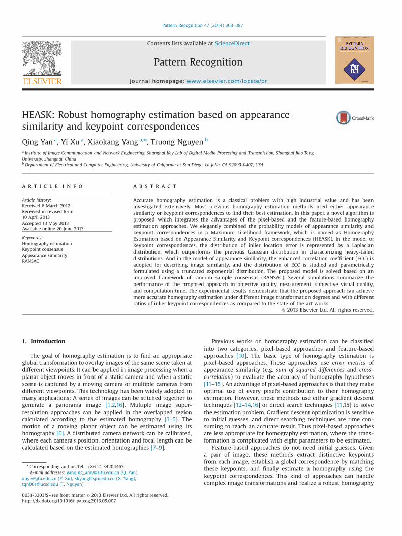
For each image pair of IR and IT , a group of keypoint corre-spondences are extracted using SURF [43]. To eliminate theinfluence of outlier, the first 50 inliers ranked according to SURFmatching scores are taken into our analysis, which produces 100inlier fitting errors (50 in horizontal direction and 50 in verticaldirection). Thus there are a total of 25000 inlier fitting errors for250 image pairs in each subinterval of transformation degree,which can well represent the statistical distribution of inlierfitting error.

The four histograms of inlier fitting error are shown in Table 1,which correspond to the four εT subintervals. To better demon-strate εT 's effect on inlier fitting error, four image pair examples arealso provided in the left column of Table 1. The extracted keypointcorrespondences ððxR; yRÞ; ðxT ; yT ÞÞ using SURF [43] are linked withred lines, and the ground truth of keypoint correspondencesððxnTR; yn

TRÞ; ðxT ; yT ÞÞ are linked with green lines, where ðxnTR; ynTRÞ

is calculated by transforming ðxT ; yT Þ according to the ground truthof θnTR. It is shown that, as the transformation degree εT increases,the extracted keypoints become less accurate, and accordingly thefitting errors become larger. From the histograms in theright column, it can be observed that inlier fitting errors aredominantly distributed around zero value and heavy-tailed dis-tributed with the increase of inlier fitting error or transformationdegree.

It is a challenge for a Gaussian model to describe such heavy-tailed distribution. However, a Laplacian model can be moresuitable for representing such distributions [44]. The fitting resultsof two models are compared in Table 1, where the red curve is theresult of Laplacian model and the green curve is the result ofGaussian model. It can be observed that the Laplacian model has abetter fitness than the Gaussian model. The fitting errors of twomodels are also compared using Kullback–Leibler (KL) divergence,which is defined as

KLðp;hÞ ¼ ∑x∈h

pðxÞlog pðxÞhðxÞ

; ð7Þ

where pðxÞ ¼ pðxÞ=ð∑s∈hðsÞÞ is the normalized fitting distributionand hðxÞ ¼ hðxÞ=ðΣs∈hhðsÞÞ is the normalized histogram. A smaller KLdivergence represents a better fit. From the calculated KL diver-gences in Table 2, it is also shown that the Laplacian modeloutperforms the Gaussian model in the distribution fitting.

3.2. Probability model of keypoint correspondences

Due to the better fitness of a Laplacian model, it is adopted inour probability model of inlier fitting error. Similar to the works ofMLESAC [34], it is assumed that the inlier fitting errors inhorizontal direction and in vertical direction are i. i. d., and theinlier fitting errors from different keypoint correspondences arealso i. i. d.. Consequently, the probability model for inlier fittingerror is a joint probability of 4Ninlier Laplacian models

pðDinlierjIR; IT ; θTRÞ ¼ ∏Ninlier

i ¼ 1

1

16b4e−

jxiTR

−xiRjþjyi

TR−yi

Rjþjxi

RT−xi

Tjþjyi

RT−yi

Tj

b ; ð8Þ

where Ninlieris the number of inliers, ðxiTR; yiTRÞ is transformedfrom ðxiT ; yiT Þ according to θTR, and ðxiRT ; yiRT Þ is transformed fromðxiR; yiRÞ according to θ−1TR. The scale parameter b is larger than zero,which is referred as the distribution diversity. For simplicity, wedenote the fitting error of jxiTR−xiRj þ jyiTR−yiRj þ jxiRT−xiT jþ jyiRT−yiT jasdisi.

If a keypoint correspondence is an outlier, its transformedkeypoints ðxiTR; yiTRÞ and ðxiRT ; yiRT Þ could locate at any position in

Table 1The distributions of inlier fitting error under different transformation degrees.

Q. Yan et al. / Pattern Recognition 47 (2014) 368–387 371

Q. Yan et al. / Pattern Recognition 47 (2014) 368–387372

the image, which follows a uniform distribution of 1=SR forðxiTR; yiTRÞ and 1=ST for ðxiRT ; yiRT Þ (SR and ST are the image area ofIR and IT ).

Thus the probability model of all keypoint correspondencesis a mixture of Laplacian distributions (8) and uniform distributions

pðDjIR; IT ; θTRÞ ¼ ∏ND

i ¼ 1γi

1

16b4e−

disib þ ð1−γiÞ

1SR⋅ST

� �; ð9Þ

where NDis the total number of keypoint correspondences, and γiis aBoolean variable indicating the inliers (γi¼1) and the outliers (γi¼0).The log likelihood of (9) is

ln pðDjIR; IT ; θTRÞ ¼ ∑Ninlier

i ¼ 1−lnð16b4Þ−disi

b

� �þ ∑

Noutlier

i ¼ 1ð−lnðSR⋅ST ÞÞ: ð10Þ

4. Probability model of appearance similarity

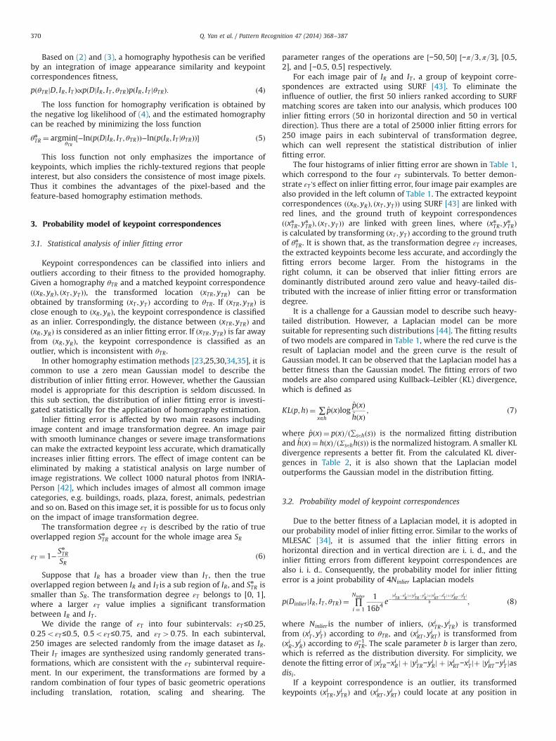
According to the pixel based image registration work of [14],the enhanced correlation coefficient (ECC) proposed in [39] was agood similarity descriptor in image alignment. Hence ECC isadopted in the proposed approach. In this section, ECC's calcula-tion is first introduced, and then the probability model of appear-ance similarity is formulated based on ECC's distribution, finallythe robustness of ECC feature is discussed.

Fig. 1. A demonstration of ECC calculation. (a) The image IT to be transformed. (b) The reIT to IRaccording to an accurate homography. (d) The transformed image ITR2 which is obblack background implies the overlapped areas (STR1 and STR2) calculated according to thtruth of overlapped region SnTR is marked with red borders in the reference image.

Table 2The KL divergences of two models under different deformation degrees.

Deformation degree KL divergence

Gaussian model Laplacian model

εT≤0:25 0.384 0.2610:25oεT≤0:5 0.597 0.4720:5oεT≤0:75 0.949 0.707εT 40:75 1.191 0.788

4.1. The ECC feature

Given a pair of image, their ECC feature can be calculated as

ECCðf;gÞ ¼ fT⋅g

jjfjj⋅jjgjj þ c; ð11Þ

where fand g are two vectors obtained by reshaping the pixels intwo images respectively, f and g are the vectors which subtractfrom f and g their corresponding arithmetic means, jjfjj is theEuclidean norm of vector f, and c is a small constant to avoid azero denominator. Here the subscript ‘T ’ is the transpose operatorof vectors.

In the application of homography estimation, ECC is calculatedbetween the reference image IR and the transformed image ITR intheir overlapped region STR. The pixels in IT that do not belong tothe overlapped region will be transformed outside the image sizeof IR. A demonstration of ECC calculation is shown in Fig. 1.

When a homography is accurately estimated, the calculatedoverlapped region STR (marked with green borders) is consistentwith the ground truth of overlapped region SnTR (marked with redborders), and IR and ITR are quite similar in STR, as shown in Fig.1(c). Otherwise, STR is different with SnTR, which makes the similaritybetween IR and ITR in STR low, as shown in Fig.1 (d).

According to the analysis in [45], a combination of a group oflocal correlations is more robust than a global correlation whenthere are nonlinear illumination changes between IT and IR. Thusthe pixels in STR are reshaped into Ksub vectors with the samelength (iiR and iiTR, i¼ 1; ⋅⋅⋅;K). And our ECC feature is a combinationof all the K local ECCs

ECC ¼ fECCiðiiR; iiTRÞ; i¼ 1⋅⋅⋅Kg ð12Þ

4.2. The formulation of probability model of appearance similarity

The probability model of appearance similarity is formulatedbased on the distribution of local ECC when images are registeredcorrectly. The registration accuracy is measured using overlap

ference image IR . (c) The transformed image ITR1, which is obtained by transformingtained according to an incorrect homography. The polygonal region centered in thee homographies. The STR1 and STR2 are marked with green borders and the ground

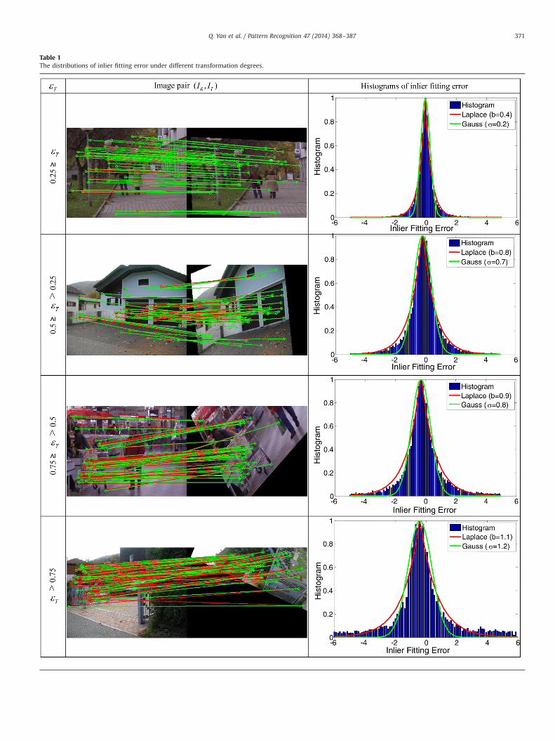
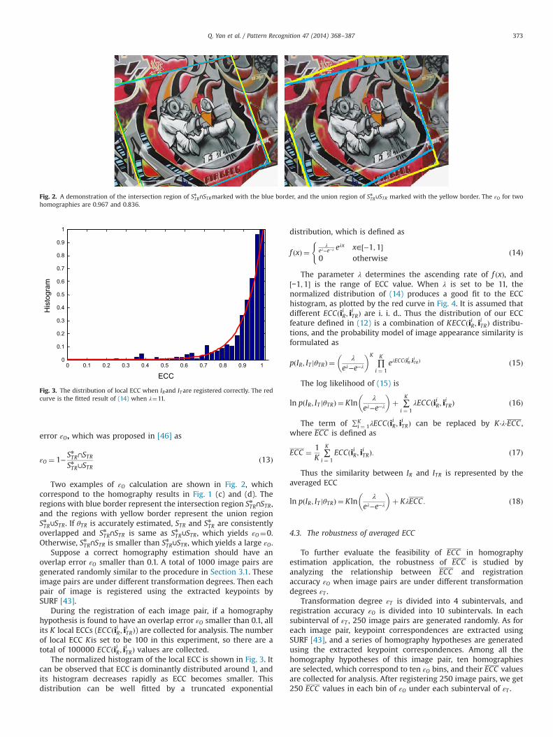
Fig. 2. A demonstration of the intersection region of SnTR∩STRmarked with the blue border, and the union region of SnTR∪STR marked with the yellow border. The εO for twohomographies are 0.967 and 0.836.

1

0 0.1 0.2 0.3 0.4 0.5 0.6 0.7 0.8 0.9 10

0.1

0.2

0.3

0.4

0.5

0.6

0.7

0.8

0.9

ECC

His

togr

am

Fig. 3. The distribution of local ECC when IRand ITare registered correctly. The redcurve is the fitted result of (14) when λ¼11.

Q. Yan et al. / Pattern Recognition 47 (2014) 368–387 373

error εO, which was proposed in [46] as

εO ¼ 1−SnTR∩STRSnTR∪STR

ð13Þ

Two examples of εO calculation are shown in Fig. 2, whichcorrespond to the homography results in Fig. 1 (c) and (d). Theregions with blue border represent the intersection region SnTR∩STR,and the regions with yellow border represent the union regionSnTR∪STR. If θTR is accurately estimated, STR and SnTR are consistentlyoverlapped and SnTR∩STR is same as SnTR∪STR, which yields εO¼0.Otherwise, SnTR∩STR is smaller than SnTR∪STR, which yields a large εO.

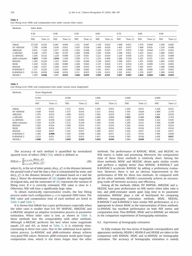
Suppose a correct homography estimation should have anoverlap error εO smaller than 0.1. A total of 1000 image pairs aregenerated randomly similar to the procedure in Section 3.1. Theseimage pairs are under different transformation degrees. Then eachpair of image is registered using the extracted keypoints bySURF [43].

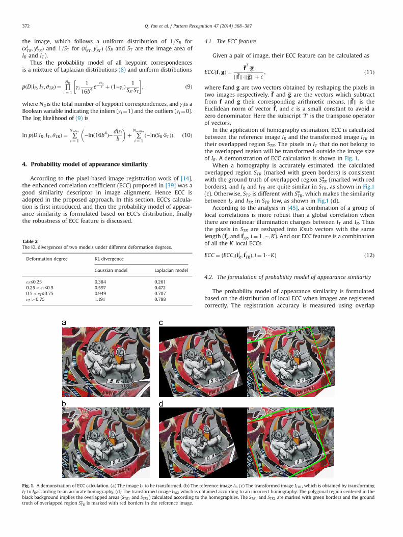
During the registration of each image pair, if a homographyhypothesis is found to have an overlap error εO smaller than 0.1, allits K local ECCs (ECCðiiR; iiTRÞ) are collected for analysis. The numberof local ECC Kis set to be 100 in this experiment, so there are atotal of 100000 ECCðiiR; iiTRÞ values are collected.

The normalized histogram of the local ECC is shown in Fig. 3. Itcan be observed that ECC is dominantly distributed around 1, andits histogram decreases rapidly as ECC becomes smaller. Thisdistribution can be well fitted by a truncated exponential

distribution, which is defined as

f ðxÞ ¼λ

eλ−e−λ eλx x∈½−1;1�

0 otherwise

(ð14Þ

The parameter λ determines the ascending rate of f ðxÞ, and½−1;1� is the range of ECC value. When λ is set to be 11, thenormalized distribution of (14) produces a good fit to the ECChistogram, as plotted by the red curve in Fig. 4. It is assumed thatdifferent ECCðiiR; iiTRÞ are i. i. d.. Thus the distribution of our ECCfeature defined in (12) is a combination of KECCðiiR; iiTRÞ distribu-tions, and the probability model of image appearance similarity isformulated as

pðIR; IT jθTRÞ ¼λ

eλ−e−λ

� �K

∏K

i ¼ 1eλECCði

iR ;i

iTRÞ ð15Þ

The log likelihood of (15) is

ln pðIR; IT jθTRÞ ¼ Klnλ

eλ−e−λ

� �þ ∑

K

i ¼ 1λECCðiiR; iiTRÞ ð16Þ

The term of ∑Ki ¼ 1λECCði

iR; i

iTRÞ can be replaced by K⋅λ⋅ECC ,

where ECC is defined as

ECC ¼ 1K

∑K

i ¼ 1ECCðiiR; iiTRÞ: ð17Þ

Thus the similarity between IR and ITR is represented by theaveraged ECC

ln pðIR; IT jθTRÞ ¼ Klnλ

eλ−e−λ

� �þ KλECC : ð18Þ

4.3. The robustness of averaged ECC

To further evaluate the feasibility of ECC in homographyestimation application, the robustness of ECC is studied byanalyzing the relationship between ECC and registrationaccuracy εO when image pairs are under different transformationdegrees εT .

Transformation degree εT is divided into 4 subintervals, andregistration accuracy εO is divided into 10 subintervals. In eachsubinterval of εT , 250 image pairs are generated randomly. As foreach image pair, keypoint correspondences are extracted usingSURF [43], and a series of homography hypotheses are generatedusing the extracted keypoint correspondences. Among all thehomography hypotheses of this image pair, ten homographiesare selected, which correspond to ten εO bins, and their ECC valuesare collected for analysis. After registering 250 image pairs, we get250 ECC values in each bin of εO under each subinterval of εT .

Q. Yan et al. / Pattern Recognition 47 (2014) 368–387374

These 250 ECCvalues are averaged to obtain the statisticallyrepresentative ECCof each εObin. The relationships between ECC andεOunder four εT subintervals are shown in Fig. 4. It can be observedthat ECC decreases as εO increases, and ECC reaches its peak when εOis close to zero and homography hypothesis is close to the groundtruth. When εT increases, there is an overall decline of ECC , but thegeneral decreasing trend is unchanged. Thus ECC is a robust feature fordescribing appearance similarity in homography estimation.

5. Implementation of HEASK framework

5.1. The loss function of HEASK

Based on the proposed probability models for keypoint corre-spondences (10) and image appearance similarity (18), the lossfunction (5) can be reformulated as

θnTR ¼ argminθ

−Klnð λ

eλ−e−λÞ−KλECC þ Ninlier lnð16b4Þ

�

þ∑Ninlieri ¼ 1

disib

þ∑Noutlieri ¼ 1 lnðSRST Þ

�; ð19Þ

which is equal to

θnTR ¼ argminθ

−Klnð λ

eλ−e−λÞ−KλECC þ NDlnð16b4Þ

�

þ∑Ninlieri ¼ 1

disib

þ∑Noutlieri ¼ 1 lnðSRST Þ−lnð16b4Þ

� ��: ð20Þ

here, the parameters λ, b and ND are chosen by user based onempirical values, so ND⋅lnð16b4Þ becomes a constant, which can beneglected in the minimization procedure. Since b is positive, it isacceptable to multiply bin (20) to yield

θnTR ¼ argminθ

−bKlnð λ

eλ−e−λÞ−bKλECC þ ð∑Ninlier

i ¼ 1 disi

�

0 0.1 0.2 0.3 0.4 0.5 0.6 0.7 0.8 0.9 10

0.1

0.2

0.3

0.4

0.5

0.6

0.7

0.8

0.9

1

EC

C

0 0.1 0.2 0.3 0.4 0.5 0.6 0.7 0.8 0.9 10

0.1

0.2

0.3

0.4

0.5

0.6

0.7

0.8

0.9

1

EC

C

Overlap Erro Oε

Overlap Error Oε

Fig. 4. The relationships of ECCand overlap error εO under different transformation

þ∑Noutlieri ¼ 1 bðlnðSRST Þ−lnð16b4ÞÞÞ

ið21Þ

The term ð∑Ninlieri ¼ 1 disi þ ∑Noutlier

i ¼ 1 bðlnðSRST Þ−lnð16b4ÞÞÞ denotes thesum of fitting errors of all keypoint correspondences. When b isempirically set to be 0.9, the value of b lnðSRST Þ−lnð16b4Þ

� �is 18.13

for the image size of 320�240. This value increases as the rise ofimage size, which equals 21.55 for the image size of 800�640. It isappropriate to use this value as the threshold for classifying inlersand outliers, since the tolerance of inlier fitting error also increasesas the rise of image size. Denote b lnðSRST Þ−lnð16b4Þ

� �as Thoutlier ,

the Eq. (21) becomes

θnTR ¼ argminθ

−bKlnλ

eλ−e−λ

� �−bλKECC þ ð∑Ninlier

i ¼ 1 disi

�

þ∑Noutlieri ¼ 1 ThoutlierÞ

i: ð22Þ

To normalize the term of keypoint fitting error, (22) is dividedby a factor of NDThoutlier

θnTR ¼ argminθ

−bKlnð λeλ−e−λÞ

NDThourlier−

bλKNDThourlier

ECC�

þ∑Ninlieri ¼ 1 disi þ∑Noutlier

i ¼ 1 Thoutlier

NDThourlier

#: ð23Þ

To ensure that the factors of appearance similarity and key-point correspondences contribute equally in (23), the term

bλKNDThourlier

ECC should also be normalized. Thus Kcan be calculated as

bλKNDThourlier

¼ 1⇒K ¼ NDThoutlierλb

: ð24Þ

Since Kcan be calculated according to (24), which is indepen-

dent with θTR, the−bKlnð λ

eλ−e−λÞ

NDThourlierterm in (23) becomes a constant. Thus

0 0.1 0.2 0.3 0.4 0.5 0.6 0.7 0.8 0.9 10

0.1

0.2

0.3

0.4

0.5

0.6

0.7

0.8

0.9

1

EC

C

0 0.1 0.2 0.3 0.4 0.5 0.6 0.7 0.8 0.9 10

0.1

0.2

0.3

0.4

0.5

0.6

0.7

0.8

0.9

1

EC

C

Overlap ErrorO

ε

Overlap Error Oε

degrees. (a) εrr0.25, (b) 0.25oεrr0.5, (c) 0.5oεrr0.75, and (d) 0.75oεr .

Q. Yan et al. / Pattern Recognition 47 (2014) 368–387 375

the final loss function of HEASK can be simplified as

θnTR ¼ argminθ

−ECC þ 1NDThoutlier

∑Ninlieri ¼ 1 disi þ∑Noutlier

i ¼ 1 Thoutlierh i�

ð25Þ

5.2. The realization framework of HEASK

The loss function (25) is optimized using a RANSAC basedframework. Due to the complex process of ITR generation in ECCcalculation, it is quite time consuming if every homographyhypothesis is verified using (25). Hence, an accelerate step isincluded in the realization framework of HEASK, which is basedon the idea of R-RANSAC.T [24].

Before the full verification of (25), a preliminary test isperformed, which evaluates the homography hypothesis on a smallsub group of keypoint correspondences. The keypoint correspon-dences in the sub group are randomly selected from D, whosenumber Nsub is much smaller than ND. Full homography verifica-tion is only performed when all Nsub keypoint correspondences areconsidered consistent with the homography hypothesis.

Based on this preliminary test, large number of homographyhypotheses is rejected if they are apparently far from the groundtruth. Thus the computing time of HEASK is dramatically reduced,while its performance is little affected. The whole framework ofHEASK is shown in Table 3, where the preliminary evaluation is instep (3.1)–(3.3) and the full verification is in step (4.1)–(4.4).

There are two terms in HEASK's loss function (25). To analyzethe two terms separately, we name the method with only the termof keypoint correspondence fitness as HEASK-I, and name themethod with only the term of image appearance similarity asHEASK-II. The realization frameworks of HEASK-I and HEASK-II aresimilar to the one of HEASK, where HEASK-I does not have step(4.2) and HEASK-II does not have step (4.1).

-10 -5 0 5 10-10

0

10

20

30

-10 -5 0 5 10-5

0

5

10

15

20

25

-

-

Fig. 5. Four examples of line fitting data. (a) ðη; sÞ¼(0.9, 0.25), (a)

Table 3The realization framework of HEASK.

Run Nitertimes:(1) Select 4 keypoint correspondences randomly(2) Fit homography θTRwith the 4 keypoint correspondences(3.1) Draw Nsubkeypoint correspondences randomly(3.2) Measure the fitting error on theNsub keypoint correspondences(3.3) If all Nsub keypoint correspondences are judged as inlier

(4.1) Calculate the fitting errors of all keypoint correspondences.(4.2) Calculate the enhanced ECC.(4.3) Calculate the cost according to (25).(4.4) If the cost is smaller than the recorded smallest costRecord θTR as the best homography, and record the cost of θTR

as the smallest cost(4.4) Go to (1)

(3.3) Go to (1)Output θnTR with the smallest cost

6. Experimental results

In this section, extensive experiments are conducted to evalu-ate HEASK's performance in different image registration situations,where the contributions of the two terms (keypoint correspon-dence term and appearance similarity term) in HEASK are inves-tigated separately.

In our probability model of keypoint correspondence, theLaplacian distribution is adopted to replace the Gaussian distribu-tion in describing the distribution of inlier fitting error. To evaluatethe performance of this model, HEASK-I is compared with twelvestate-of-the-art parameter estimation methods, which are pre-viously applied to line fitting.

Three methods which demonstrate promising performance inline fitting are selected in the comparison of image homographyestimation. To evaluate the contributions of our two terms,HEASK-I, HEASK-II and HEASK are altogether taken in the compar-ison of homography estimation. The image pairs adopted in thecomparison are under different transformation degrees and withdifferent inlier keypoint correspondence ratios.

Finally, computation time analysis of HEASK and its applicationin panorama synthesis are provided. Consistent performance ofHEASK can be expected using common parameter settings fordifferent image pairs. For all the experiments in this section, theparameters ND, b and λ in (14) are empirically set to be 50, 0.9 and11 respectively. The parameter Nsub in Table 3 is set to be 4.

6.1. Experiments of linear fitting

The twelve methods adopted in this comparison include atraditional statistical method (LMeds [21]) and eleven methodsfrom RANSAC family, where the RANSAC family methods can bedivided into four categories according to [47]. RANSAC [19], MSAC[34] and MLESAC [34] are three approaches with modified lossfunctions in their verification process. Lo-RANSAC [40] and pbM-estimator [36] added a local optimization process to RANSAC foraccuracy improvement. FH’ MAPSAC [48], AMLESAC [49] andu-MLESAC [50] employed an adaptive termination process toterminate estimation iteration. R-RANSAC.T [24] and R-RANSAC.S[26] introduced a preliminary evaluation to reduce the number ofcomplete verifications. These methods typically represent thestate-of-the-art parameter estimation approaches.

In the line fitting experiments, two hundred points are gener-ated randomly, where inliers are from the line of 0:8xþ0:6y−5:0¼ 0 (x∈½−10;10� and y∈½−5;21:67�) with unbiased Gaus-sian noise, and outliers are uniformly distributed in the space ofðx; yÞ. Experiments are performed on the sets with various inlierratio η and noise magnitude s, where η∈f0:3;0:4;0:5;0:6;0:7;0:8;0:9g and s∈f0:25;0:5;1:0;2:0;4:0g. Four examples underdifferent configurations of ðη; sÞ are shown in Fig. 5. It is shownthat more points are concentrated along the line with the increaseof η. As s increases, inlier points become more scattered aroundthe true line.

-10 -5 0 5 1020

10

0

10

20

30

-10 -5 0 5 10-5

0

5

10

15

20

25

ðη;sÞ¼(0.3, 0.5), (c) ðη; sÞ¼(0.9, 4.0) and (d) ðη; sÞ¼(0.5, 2.0).

Table 4Line fitting error (NSE) and computation time under various inlier ratios.

Methods Inlier Ratio

0.30 0.40 0.50 0.60 0.70 0.80 0.90

NSE Time (s) NSE Time (s) NSE Time (s) NSE Time (s) NSE Time (s) NSE Time (s) NSE Time (s)

LMeds 27.320 0.226 6.461 0.094 1.321 0.047 1.356 0.025 1.408 0.015 1.379 0.009 1.509 0.005FH’ MAPSAC 7.708 0.046 2.036 0.052 1.647 0.038 1.484 0.024 1.463 0.015 1.490 0.010 1.526 0.006AMLESAC 2.051 1.336 1.477 0.520 1.452 0.248 1.529 0.129 1.517 0.072 1.526 0.044 1.575 0.025u-MLESAC 5.246 1.072 1.382 0.139 1.402 0.068 1.383 0.036 1.398 0.021 1.433 0.012 1.489 0.007Lo-RANSAC 1.245 0.232 1.229 0.098 1.229 0.051 1.221 0.029 1.229 0.018 1.253 0.012 1.255 0.008pbM-estimator 1.023 3.390 1.034 1.438 1.209 0.731 1.255 0.406 1.286 0.236 1.291 0.155 1.355 0.091RANSAC 1.305 0.220 1.323 0.091 1.326 0.046 1.330 0.025 1.390 0.015 1.415 0.009 1.483 0.005MSAC 1.229 0.216 1.266 0.089 1.284 0.045 1.337 0.024 1.373 0.014 1.415 0.009 1.535 0.005MLESAC 1.248 0.257 1.269 0.107 1.289 0.053 1.316 0.029 1.358 0.017 1.410 0.011 1.446 0.006R-RANSAC.T 1.317 0.220 1.323 0.091 1.304 0.045 1.341 0.011 1.394 0.008 1.401 0.006 1.475 0.005R-RANSAC.S 15.210 0.038 1.848 0.052 1.131 0.055 1.229 0.012 1.291 0.011 1.370 0.017 1.389 0.029HEASK-I 1.205 0.046 1.097 0.032 1.062 0.019 1.055 0.011 1.057 0.007 1.062 0.004 1.068 0.003

Table 5Line fitting error (NSE) and computation time under various noise magnitudes

Methods Noise Magnitude

0.250 0.500 1.000 2.000 4.000

NSE Time (s) NSE Time (s) NSE Time (s) NSE Time (s) NSE Time (s)

LMeds 1.379 0.015 1.372 0.015 1.295 0.015 1.256 0.015 1.228 0.015FH’ MAPSAC 1.458 0.015 1.557 0.014 1.513 0.012 1.395 0.029 1.406 2.379AMLESAC 1.479 0.072 1.499 0.072 1.942 0.070 1.192 0.072 1.164 0.078u-MLESAC 1.361 0.021 1.232 0.027 1.069 0.084 1.025 0.486 1.051 2.763Lo-RANSAC 1.219 0.018 1.224 0.018 1.202 0.018 1.203 0.018 1.222 0.018pbM-estimator 1.258 0.239 1.272 0.244 1.264 0.243 1.296 0.221 1.306 0.208RANSAC 1.385 0.014 1.380 0.014 1.315 0.014 1.282 0.014 1.259 0.014MSAC 1.389 0.014 1.319 0.014 1.306 0.014 1.246 0.014 1.193 0.014MLESAC 1.364 0.017 1.341 0.017 1.309 0.017 1.262 0.017 1.218 0.017R-RANSAC.T 1.396 0.008 1.363 0.009 1.286 0.011 1.232 0.013 1.180 0.020R-RANSAC.S 1.253 0.011 1.325 0.013 1.413 0.044 1.583 0.036 1.618 0.011HEASK-I 1.046 0.011 1.043 0.010 1.043 0.010 1.084 0.010 1.218 0.012

Q. Yan et al. / Pattern Recognition 47 (2014) 368–387376

The accuracy of each method is quantified by normalizedsquared error of inliers (NSE) [50], which is defined as

NSEðθÞ ¼ ∑ðxi ;yiÞ∈Dindisðyi; yθi Þ∑ðxi ;yiÞ∈Din

disðyi; yn

i Þ; ð26Þ

where Din is the set of inlier points, disðyi; yn

i Þ is the distance betweenthe ground truth ynand the data y that is contaminated by noise, anddisðyi; yθi Þ is the distance between yθ calculated based on θ and thedata y. Hence the denominator of (26) implies the noise magnitudeof original data, and the numerator of (26) represents the variance offitting error. If θ is correctly estimated, NSE value is close to 1.Otherwise, NSE will have a significantly large value.

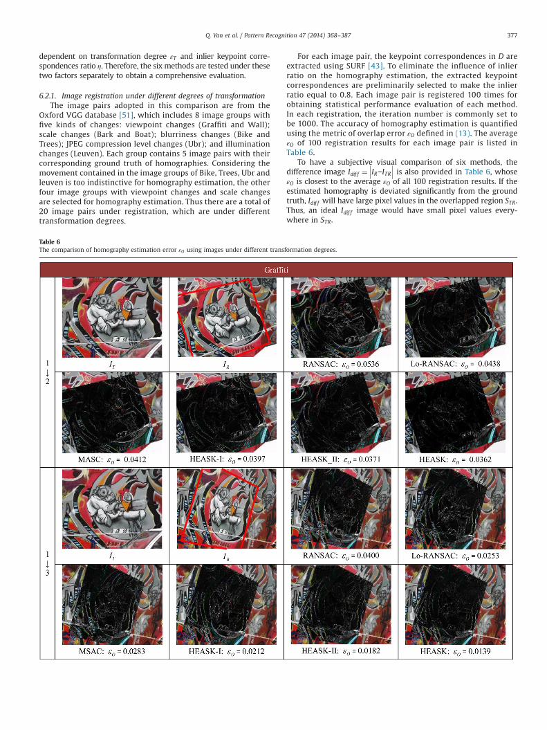
To obtain statistically representative results, the line fittingprocess under each configuration ðγ; sÞ is repeated 1000 times. TheNSE value and computation time of each method are listed inTable 4 and Table 5.

It is shown that LMeds has a poor performance especially whenthe inlier ratio is smaller than 0.4. FH’ MAPSAC, AMLESAC andu-MLESAC adopted an adaptive termination process in parameterestimation. When inlier ratio is low, as shown in Table 4,these methods lose the comparability with other methods.Although u-MLESAC performs the best when noise magnitudeequals 2.0 and 4.0, as listed in Table 5, it is relatively time-consuming in these two cases. Due to the additional local optimi-zation process, Lo-RANSAC and pbM-estimator always achievevery good NSE values. However, pbM-estimator needs quite longercomputation time, which is ten times longer than the other

methods. The performance of RANSAC, MSAC, and MLESAC onNSE metric is stable and promising. Moreover, the computationtime of these three methods is relatively short. Among thethree methods, MSAC and MLESAC obtain quite similar resultsand perform a slightly better than RANSAC. R-RANSAC.T andR-RANSAC.S accelerate RANSAC by adding a preliminary evalua-tion. However, there is not an obvious improvement in theperformance of NSE for these two methods. As compared withall the other methods, HEASK-I consistently achieve an encoura-ging trade-off between accuracy and efficiency.

Among all the methods, LMeds, FH’ MAPSAC, AMLESAC and u-MLESAC have poor performance on NSE metric when inlier ratio islow, and pbM-estimator needs quite long time in its parameterestimation. RANSAC plays a role of benchmark for comparingdifferent homography estimation methods. MSAC, MLESAC,R-RANSAC.T and R-RANSAC.S have similar NSE performance, so it isappropriate to choose MSAC as the representation of these methods.Lo-RANSAC has excellent performance on both NSE metric andcomputation time. Thus RANSAC, MSAC and Lo-RANSAC are selectedin the comparison experiments of homography estimation.

6.2. Experiments of homography estimation

To fully evaluate the two terms of keypoint correspondence andappearance similarity, HEASK-I, HEASK-II and HEASK are taken in thecomparison with RANSAC, MSAC and Lo-RANSAC on homographyestimation. The accuracy of homography estimation is mainly

Q. Yan et al. / Pattern Recognition 47 (2014) 368–387 377

dependent on transformation degree εT and inlier keypoint corre-spondences ratio η. Therefore, the six methods are tested under thesetwo factors separately to obtain a comprehensive evaluation.

6.2.1. Image registration under different degrees of transformationThe image pairs adopted in this comparison are from the

Oxford VGG database [51], which includes 8 image groups withfive kinds of changes: viewpoint changes (Graffiti and Wall);scale changes (Bark and Boat); blurriness changes (Bike andTrees); JPEG compression level changes (Ubr); and illuminationchanges (Leuven). Each group contains 5 image pairs with theircorresponding ground truth of homographies. Considering themovement contained in the image groups of Bike, Trees, Ubr andleuven is too indistinctive for homography estimation, the otherfour image groups with viewpoint changes and scale changesare selected for homography estimation. Thus there are a total of20 image pairs under registration, which are under differenttransformation degrees.

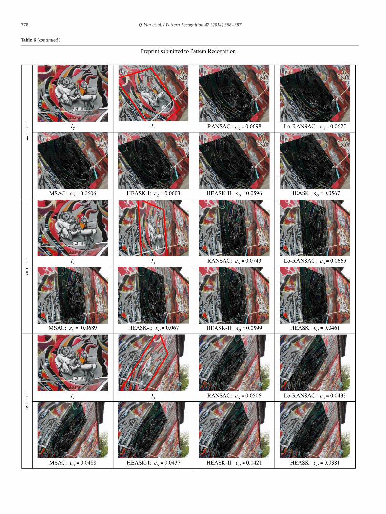
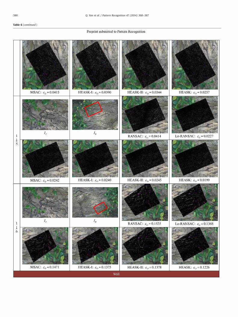
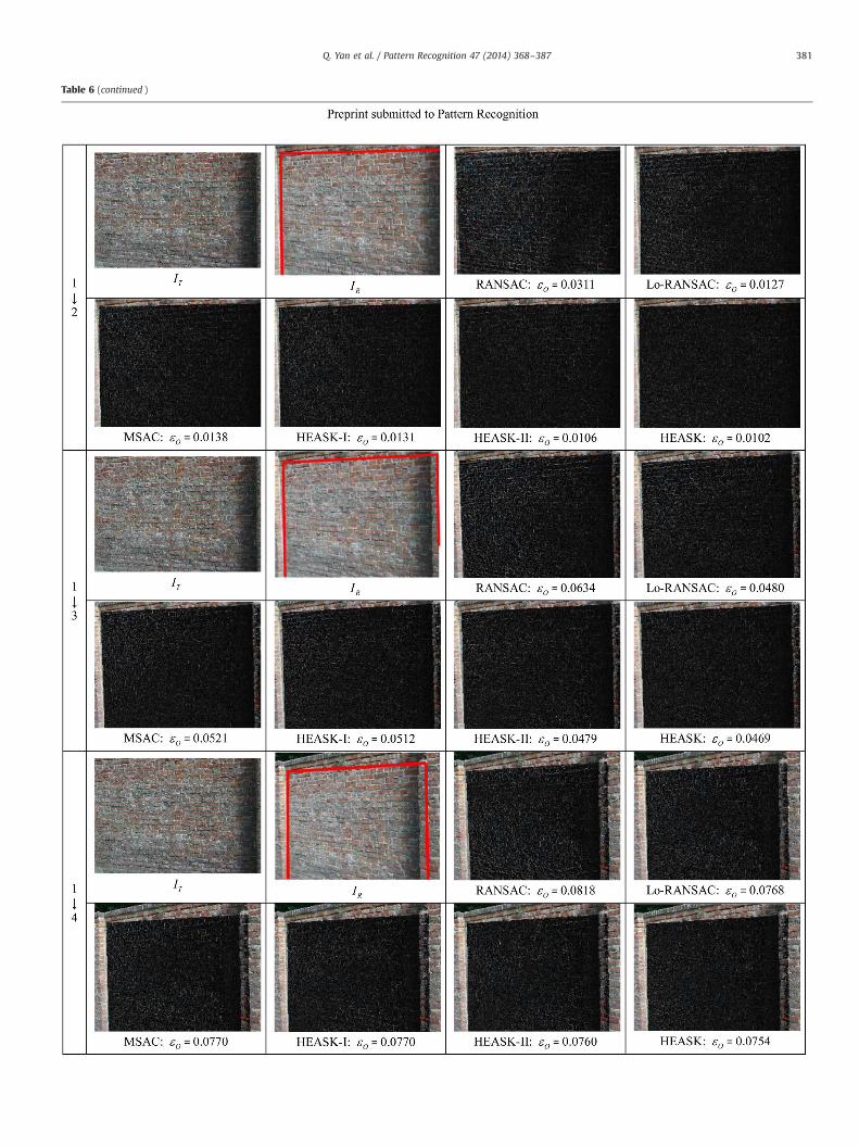
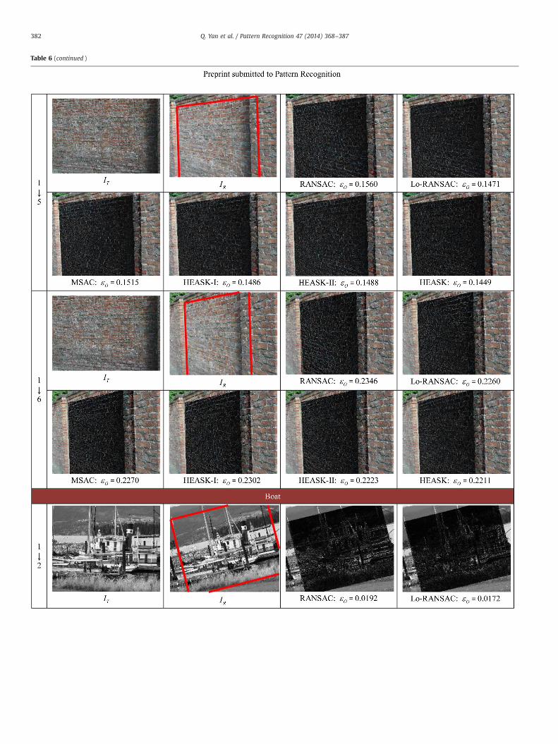
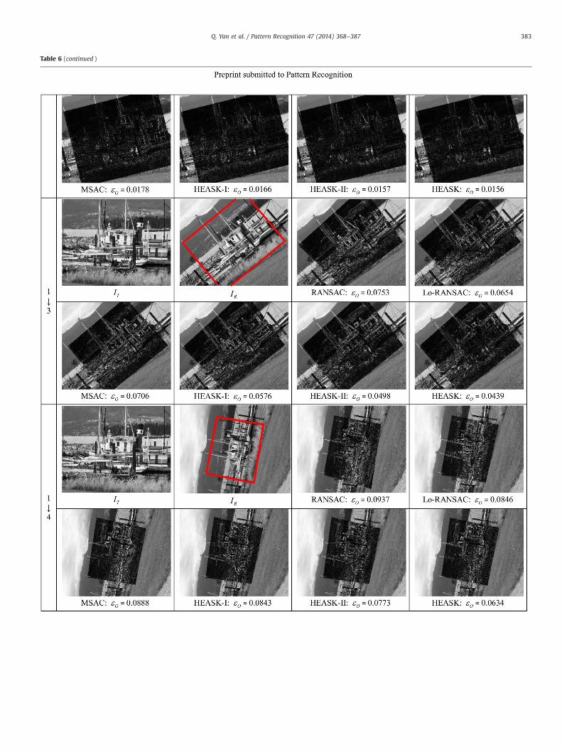
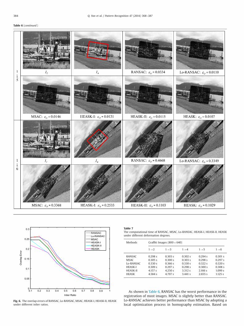
Table 6The comparison of homography estimation error εO using images under different trans

For each image pair, the keypoint correspondences in D areextracted using SURF [43]. To eliminate the influence of inlierratio on the homography estimation, the extracted keypointcorrespondences are preliminarily selected to make the inlierratio equal to 0.8. Each image pair is registered 100 times forobtaining statistical performance evaluation of each method.In each registration, the iteration number is commonly set tobe 1000. The accuracy of homography estimation is quantifiedusing the metric of overlap error εO defined in (13). The averageεO of 100 registration results for each image pair is listed inTable 6.

To have a subjective visual comparison of six methods, thedifference image Idif f ¼

IR−ITR is also provided in Table 6, whoseεO is closest to the average εO of all 100 registration results. If theestimated homography is deviated significantly from the groundtruth, Idif f will have large pixel values in the overlapped region STR.Thus, an ideal Idif f image would have small pixel values every-where in STR.

formation degrees.

Table 6 (continued )

Q. Yan et al. / Pattern Recognition 47 (2014) 368–387378

Table 6 (continued )

Q. Yan et al. / Pattern Recognition 47 (2014) 368–387 379

Table 6 (continued )

Q. Yan et al. / Pattern Recognition 47 (2014) 368–387380

Table 6 (continued )

Q. Yan et al. / Pattern Recognition 47 (2014) 368–387 381

Table 6 (continued )

Q. Yan et al. / Pattern Recognition 47 (2014) 368–387382

Table 6 (continued )

Q. Yan et al. / Pattern Recognition 47 (2014) 368–387 383

Table 6 (continued )

0.1 0.2 0.3 0.4 0.5 0.6 0.7 0.8 0.9 10

0.05

0.1

0.15

0.2

0.25

0.3

Inlier Ratio

Ove

rlap

Err

or

RANSACLo-RANSACMSACHEASK-IHEASK-IIHEASK

Fig. 6. The overlap errors of RANSAC, Lo-RANSAC, MSAC, HEASK-I, HEASK-II, HEASKunder different inlier ratios.

Table 7The computational time of RANSAC, MSAC, Lo-RANSAC, HEASK-I, HEASK-II, HEASKunder different deformation degrees.

Methods Graffiti Images (800�640)

1-2 1-3 1-4 1-5 1-6

RANSAC 0.298 s 0.303 s 0.302 s 0.294 s 0.301 sMSAC 0.305 s 0.300 s 0.303 s 0.298 s 0.297 sLo-RANSAC 0.330 s 0.366 s 0.330 s 0.322 s 0.320 sHEASK-I 0.309 s 0.297 s 0.298 s 0.300 s 0.308 sHEASK-II 4.157 s 4.250 s 3.312 s 2.166 s 1.099 sHEASK 4.584 s 4.797 s 3.441 s 2.655 s 1.125 s

Q. Yan et al. / Pattern Recognition 47 (2014) 368–387384

As shown in Table 6, RANSAC has the worst performance in theregistration of most images. MSAC is slightly better than RANSAC.Lo-RANSAC achieves better performance than MSAC by adopting alocal optimization process in homography estimation. Based on

Fig. 7. Panorama synthesis. (a) A series of images obtained by rotating a static camera horizontally in front of a building. (b) The stitched image based on the homographyestimations of HEASK. (c) The panorama obtained after geometric rectification on (b).

Q. Yan et al. / Pattern Recognition 47 (2014) 368–387 385

the improved model of keypoint correspondences, HEASK-I alwayshas better or comparable performance as compared with Lo-RANSAC. By taking image appearance similarity into consideration,HEASK-II outperforms HEASK-I in most cases. However, whenthere are many pixels with smooth luminance changes in STR, e.g. the second image group (Bark), HEASK-II may generate anunreliable homography due to ambiguity among the similar pixels.HEASK achieves a good trade-off between keypoint correspon-dences and image similarity, which consistently performs best inall the image registrations.

6.2.2. Image registration under different inlier ratiosAs for the experiments in 6.2.1, it is assumed there are 80%

inlier keypoint correspondences in the dataset D. In this subsection, RANSAC, Lo-RANSAC, MSAC, HEASK-I, HEASK-II andHEASK are evaluated when D has different inlier ratios.

The total number of keypoint correspondences in D is empiri-cally set to be 50. And the range of inlier ratio η is divided into 10

subintervals. In each subinterval, 100 image pairs are generatedusing the dataset of INRIAPerson [42]. The homographies of the100 image pairs are generated randomly, which is similar to theprocedure in Section 3.1. For each image pair, keypoint correspon-dences are extracted using SURF [43]. Then the keypoint corre-spondences are separated into inliers and outliers according to theground truth of homography. Finally, a certain number of inliersand outliers are selected randomly to comprise D and meet the ηsubinterval requirement.

The iteration number is set to be 2000 for all the methods. Theaccuracy of homography estimation using each method is evaluatedusing overlap errorεO. The relationship between εO and η is depictedusing average εO in each η subinterval, as shown in Fig. 6. It isobserved that the performance of RANSAC and MSAC is worse thanthe other methods due to their simple verification functions. Lo-RANSAC achieves a better performance by introducing a localoptimization process. Without the local optimization, HEASK-I stillachieves comparable performance to Lo-RANSAC by employing theLaplacian distribution to model inlier fitting error. Appearance

Q. Yan et al. / Pattern Recognition 47 (2014) 368–387386

similarity is another important factor to improve the accuracy ofhomography estimation. Therefore, HEASK-II is comparable or evenbetter than most of the keypoint correspondence based methods.By taking both keypoint correspondences and appearance similarityinto consideration, HEASK always achieves the best performanceespecially when the inlier ratio is smaller than 0.4.

6.3. Computational time analysis

A comparison of computational time is made to evaluate theefficiency of homography estimation methods. We provide theimage registration time of Graffiti group images, where the imagesize is 800�640 and the transformation degree increases as the IRindex grows. Each image pair is registered 100 times to obtainstatistical representative result. The iteration number of eachregistration is set to be 1000. All the experiments are realizedusing Matlab platform on a PC with Intels Core™ 2 Duo CPUE6550@2.33 GHz.

The computational time is shown in Table 7. Since the totalnumber of keypoint correspondences in D is set to be 50, thecomputational time of RANSAC, MSAC, Lo-RANSAC and HEASK-Ichanges slightly for image pairs under different transformationdegrees. Since Lo-RANSAC added a local optimization process, itscomputation time is a little longer than the other three feature-based approaches. Due to the calculation of ECC, HEASK-II andHEASK are more time consuming than the four feature-basedmethods. As the transformation degree increases, keypoint corre-spondences are contaminated with more significant noise. In thiscase, more homography hypotheses are rejected by the prelimin-ary evaluation in step (3.1) in Table 4, which reduces the computa-tion time of HEASK-II and HEASK, as shown in Table 7. Consideringthe good accuracy of HEASK, the computation time of HEASK isacceptable in many off-line applications.

6.4. Application in panorama synthesis

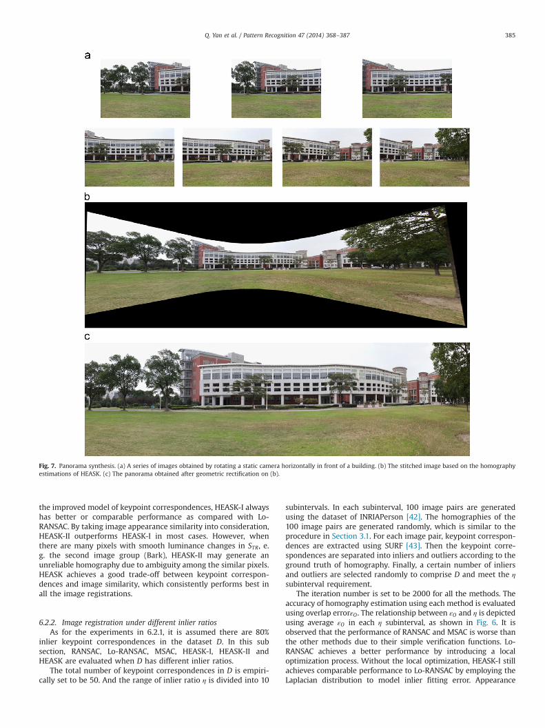
An application of panorama synthesis is also provided in thispaper. Given a series of images, a panorama image can be obtainedby registering the images pair by pair based on the homographyestimations of HEASK. An example is shown in Fig. 7. Fig. 7 (a)provides seven images, which are obtained by rotating a staticcamera horizontally in front of a building. Taking the fourth imagein Fig. 7 (a) as the reference image, the other images are transformedto the reference image pair by pair according to the estimatedhomographies. Then the stitched image is generated as shown inFig. 7 (b). It can be observed, the seven images are stitched togetherseamlessly, so the homographies estimated by the proposed algo-rithm are very accurate. After a geometrical correction on thestitched image, a panorama image can be obtained as shown inFig. 7 (c).

7. Conclusion

In this paper, we propose a novel homography estimationalgorithm. It integrates models of keypoint correspondences andappearance similarity in a Maximum Likelihood framework, which isnamed as HEASK (Homography Estimation based on AppearanceSimilarity and Keypoint correspondences). In the model of keypointcorrespondences, the distribution of inlier location error is repre-sented by a Laplacian distribution, which outperforms a Gaussiandistribution in characterizing heavy-tailed distributions. In the modelof appearance similarity, the similarity between the reference imageand the transformed image is represented by ECC feature. Thedistribution of ECC is parametrically described by a truncatedexponential distribution. We realize our algorithm in a RANSAC

based framework. Our algorithm can consistently achieve an accuratehomography estimation under different transformation degrees anddifferent inlier ratios. The performance of HEASK is highlighted bythe experimental results in both objective quality measurement andsubjective visual quality.

Acknowledgments

Art of this work has been accepted by ICME2012. This work wassupported in part by Research Fund for the Doctoral Program of HigherEducation of China(20090073110022), NSFC (60932006, 60902073,61025005), 973 Program (2010CB721401, 2010CB721406), and Qual-comm sponsored project ‘Super-resolution based on dual camerasystem’.

References

[1] R. Szeliski, H.-Y. Shum, Creating full view panoramic image mosaics andtexture-mapped models, in: Proceedings of the Computer Graphics,SIGGRAPH'97, 1997, pp. 251–258.

[2] Y. He, R. Chung, Image mosaicking for polyhedral scene and in particular singlyvisible surfaces, Pattern Recognition 31 (2008) 1200–1213.

[3] A. Akyol, M. Gökmen, Super-resolution reonstruction of faces by enhancedglobal models of shape and texture, Pattern Recognition 45 (2012) 4103–4116.

[4] H. Huang, H.T. He, X. Fan, J.P. Zhang, Super-resolution of human face imageusing canonical correlation analysis, Pattern Recognition 43 (2010)2532–2543.

[5] K. Jia, S.G. Gong, Hallucinating multiple occluded face images of differentresoltuions, Pattern Recognition Letters 27 (2006) 1768–1775.

[6] O. Deniz, G. Bueno, E. Bermejo, R. Sukthankar, Fast and accruate global motioncompensation, Pattern Recognition 44 (12) (2011) 2887–2901.

[7] E. Montijano, C. Sagues, Distributed multi-camera visual mapping usingtopological maps of planar regions, Pattern Recognition 44 (7) (2011)1528–1539.

[8] J. Su, R. Chung, L. Jin, Homography-based partitionng of curved surface forstereo correspondence establishment, Pattern Recognition Letters 28 (12)(2007) 1459–1471.

[9] T.T. Santos, C.H. Morimoto, Multiple camera people detection and trackingusing support integration, Pattern Recognition Letters 32 (1) (2011) 47–55.

[10] R. Szeliski, Image alignment and stitching: a tutorial, Foundations and Trendsin Computer Graphics and Vision 2 (1) (2006) 1–104.

[11] J. R. Bergen, P. Anandan, K. J. Hanna, R. Hingorani, Hierarchical model-basedmotion estimation, in: Proceedings of the Second European Conference onComputer Vission, 1992, pp. 237–252.

[12] S. Baker, I. Matthews, Lucas-Kanade 20 years on: a unifying framework: Part 1:The quantity approximated, the warp update rule and the gradient decentapproximation, International Journal of Computer Vision 56 (2004) 221–255.

[13] J. Kim, V. Kolmogorov and R. Zabih, Visual correspondence using energyminimization and mutual information, in: Proceedings of the Ninth Interna-tional Conference on Computer Vision, 2003, pp. 1033–1040.

[14] G.D. Evangelidis, E.Z. Psarakis, Parametric image alignment using enhancedcorrelation coefficient maximization, IEEE Transactions on Pattern Analysisand Machine Intelligence 30 (10) (2008) 1858–1865.

[15] K. Ga, Z. W. Shi, C. S. Zhang, Blind separation of superimposed images withunknown motions, in: Proceedings of the 2009 IEEE Computer SocietyConference on Computer Vision and Pattern Recognition, 2009, pp. 1881–1888.

[16] M. Brown, D.G. Lowe, Automatic panoramic image stitching using invariantfeatures, International Journal of Computer Vision (2007) 59–73.

[17] D.G. Lowe, Distinctive image features from scale-invariant keypoints, Interna-tional Journal of Computer Vision 60 (2) (2004) 91–110.

[18] H. Bay, A. Ess, T. Tuytelaars, L.V. Gool, Surf: speeded up robust features,Computer Vision and Image Understanding (CVIU) 110 (3) (2008) 346–359.

[19] M.A. Fischler, R.C. Bolles, Random sample consensus: a paradigm for modelfitting with applications to image analysis and automated cartography,Communications of the ACM 24 (6) (1981) 381–395.

[20] Proceeding IEEE International Workshop “25 years of RANSAC” in Conjunctionwith CVPR 2006, RANSAC25'06, ⟨http://cmp.felk.cvut.cz/ransac-cvpr2006/⟩.

[21] P.J. Rousseeuw, Least median of squares regression, Journal of the AmericanStatistical Association 79 (1984) 871–880.

[22] R.O. Duda, P.E. Hart, Use of the Hough transormation to detect lines and curvesin pictures, Communications of the ACM 15 (1972) 11–15.

[23] R. Raguram, J.-M. Frahm, M. Pollefeys, Exploiting uncertainty in randomsample consensus, in: Proceedings of the IEEE 12th International Conferenceon Computer Vision, 2009, pp. 2074–2081.

[24] O. Chum, J. Matas, Randomized ransac with t(d,d) test, in: Proceedings of theBritish Machine Vision Conference, BMVC, 2, 2002, pp. 448–457.

[25] D. Capel, An effective bail-out test for ransac consensus scoring, in: Proceed-ings of the British Machine Vision Conference, BMVC, 2005, pp. 629–638.

Q. Yan et al. / Pattern Recognition 47 (2014) 368–387 387

[26] J. Matas, O. Chum, Randomized ransac with sequential probability ratio test,in: Proceedings of the 10th IEEE International Conference on Computer Vision,vol. 2, 2005, pp. 1727–1732.

[27] O. Chum, J. Matas, Optimal randomized ransac, IEEE Transactions on PatternAnalysis and Image Understanding 30 (8) (2008) 1472–1482.

[28] C.-M Cheng, S.-H. Lai, A consensus sampling technique for fast and robustmodel fitting, Pattern Recognition 42 (7) (2009) 1318–1329.

[29] J.-H. Kim, J.H. Han, Outlier correction from uncalibrated image sequence usingthe trangulation method, Pattern Recognition 39 (3) (2006) 394–404.

[30] B. Tordoff, D. W. Murray, Guided sampling and consensus for motionestimation, in: Proceedings of the European Conference on Computer Vision,vol. 1, 2002, pp. 82–98.

[31] O. Chum, J. Matas, Matching with prosac-progressive sample consensus, in:IEEE Computer Society Conference on Computer Vision and Pattern Recogni-tion, Part 1, 2005, pp. 220–226.

[32] R. Raguram, J.-M. Frahm, M. Pollefeys, A comparative analysis of ransactechniques leading to adaptive real-time random sample consensus, in:Proceedings of the 10th European Coference on Computer Vision, Part 2,2008, pp. 500–513.

[33] E. Serradell, M. Zuysal, V. Lepetit, P. Fua, F. Moreno-Noguer, Combinggeometric and appearance priors for robust homography estimation, in:Proceedings of the 11th European Conference on Computer Vision, Part 3,2010, pp. 58–72.

[34] P.H.S. Torr, A. Zisserman, MLESAC: a new robust estimator with application toestimating image geometry, Computer Vision and Image Understanding 78 (1)(2000) 138–156.

[35] P.H.S. Torr, Bayesian model estimation and selection for epipolar geometryand generic manifold fitting, International Journal of Computer Vision 50 (1)(2002) 35–61.

[36] R. Subbarao, P. Meer, Subspace estimation using projection-based M-estimatorover grassmann manifolds, in: Proceedings of the 9th European Conference onComputer Vision, 2006, pp. 301–312.

[37] A. Criminisi, I. Reid, A. Zisserman, A plane measuring device, Image and VisionComputing 17 (8) (1999) 625–634.

[38] O. Chum, T. Werner, J. Matas, Two-view geometry estimation unaffected by adominant plane, in: Proceedings of the 2005 IEEE Computer Society

Conference on Computer Vision and Pattern Recognition, Part 1, 2005,pp. 772–779.

[39] E. Z. Psarakis, G. D. Evangelidis, An enhanced correlation-based method forstereo correspondence with sub-pixel accuracy, in: Proceedings of the 10thIEEE International Conference on Computer Vision, Part 1, 2005, pp. 907–912.

[40] O. Chum, J. Matas, S. Obdrzalek, Enhancing RANSAC by generalized modeloptimization, in: Proceedings of the Asian Conference on Computer Vision,ACCV, 2004.

[41] F. Moreno-Noguer, V. Lepetit, P. Fua, Pose priors for simultaneously solvingalignment and correspondence, in: Proceedigns of the 10th European Con-ference on Computer Vision: Part II, ECCV, 5303, 2008, pp. 405–418.

[42] INRIAPerson: ⟨http://pascal.inrialpes.fr/data/human/⟩.[43] Chris evans development, the opensurf computer vision library: ⟨http://www.

chrisevansdev.com/computer�vision-opensurf.html⟩.[44] J. Huang, D. Mumford, Statistics of natural images and models, in: IEEE

Computer Society Conference on Computer Vision and Pattern Recognition,vol. 2, 1999, pp. 637–663.

[45] B. Sarel, M. Irani, Separating transparent layers through layer informationexchange, in: Proceedings of the 8th European Conference on ComputerVision, vol. 3024, 2004, pp. 328–341.

[46] K. Mikolajczyk, T. Tuytelaars, C. Schmid, A. Zisserman, A comparison of affineregion detectors, International Journal of Computer Vision 65 (2005) 43–72.

[47] S. Choi, T. Kim, W. Yu, Performance evaluation of RANSAC family, in:Proceedings of the British Machine Vision Conference, BMVC, 2009.

[48] C. L. Feng and Y. S. Hung, A robust method for estimating the fundamentalmatrix, in: Proceedings of the 7th Digital Image Computing: Techniques andApplications, 2003, pp. 633–642.

[49] A. Konouchine, V. Gaganov and V. Veznevets, AMLESAC: a new maximumlikelihood robust estimator, in: Proceedings of the International Conferenceon Computer Graphics and Vison, 2005.

[50] S. Choi, J-H. Kim, Robust regression to varying data distribution and itsapplication to landmark-based localization, in: Proceedings of the IEEEConference on Systems, Man and Cybernetics, 2008.

[51] Oxford visual geometry group affine covariant regions datasets: ⟨http://www.robots.ox.ac.uk/�vgg/data/data-aff.html⟩.

Qing Yan received the B. E. degree in information engineering form China University of Mining and Technology, Xuzhou, China, in 2007, the M. E. degree in informationengineering from Shanghai Jiao Tong University, Shanghai, China, in 2009. She is currently pursuing the Ph.D. degree in information engineering in Shanghai Jiao TongUniversity. Her research interest includes image registration, superimposed image separation, and intelligent video analysis.

Yi Xu received her B. S. and M. S. degrees from Nanjing University of Science and Technology, Nanjing, China, in 1996 and 1999 respectively, and her Ph.D. degree fromShanghai Jiao Tong University, Shanghai China, in 2005. She is currently an associate professor in the Institute of Image Communication and Network Engineering,Department of Electronic Engineering, Shanghai Jiao Tong University, Shanghai, China. Her research interests include Image Processing, Intelligent Video Analysis, QuaternionWavelet Theory and Application.

Xiaokang Yang received the B. S. degree from Xiamen University, Xiamen, China, in 1994, the M. S. degree from Chinese Academy of Sciences, Shanghai, China, in 1997, andthe Ph.D. degree from Shanghai Jiao Tong University, Shanghai, China, in 2000.He is currently a professor and Vice Dean, School of Electronic Information and Electrical Engineering, and the deputy director of the Institute of Image Communication

and Information Processing, Shanghai Jiao Tong University, Shanghai, China. From August 2007 to July 2008, he visited the Institute for Computer Science, University ofFreiburg, Germany, as an Alexander von Humboldt Research Fellow. From September 2000 to March 2002, he worked as a Research Fellow in Centre for Signal Processing,Nanyang Technological University, Singapore. From April 2002 to October 2004, he was a Research Scientist in the Institute for Infocomm Research (I2R), Singapore. He haspublished over 150 refereed papers, and has filed 30 patents. His current research interests include visual signal processing and communication, media analysis and retrieval,and pattern recognition.He received National Science Fund for Distinguished Young Scholars in 2010, Professorship Award of Shanghai Special Appointment (Eastern Scholar) in 2008, the

Microsoft Young Professorship Award in 2006, the Best Young Investigator Paper Award at IS and T/SPIE International Conference on Video Communication and ImageProcessing (VCIP2003) and awards from A-STAR and Tan Kah Kee foundations. He is currently a member of Editorial Board of IEEE Signal Processing Letters, Serias Editor ofSpringer CCIS, a member of APSIPA, a senior member of IEEE, a member of Visual Signal Processing and Communications (VSPC) Technical Committee of the IEEE Circuits andSystems Society. He was the special session chair of Perceptual Visual Processing of IEEE ICME2006. He was the technical program co-chair of IEEE SiPS2007 and the technicalprogram co-chair of 3DTV workshop in junction with 2010 IEEE International Symposium on Broadband Multimedia Systems and Broadcasting.

Truong Nguyen [F'05] is currently a Professor at the ECE Dept., UCSD. His current research interests are 3D video processing and communications and their efficientimplementation. He is the coauthor (with Prof. Gilbert Strang) of a popular textbook, Wavelets & Filter Banks, Wellesley-Cambridge Press, 1997, and the author of severalmatlab-based toolboxes on image compression, electrocardiogram compression and filter bank design. He has over 300 publications. Prof. Nguyen received the IEEETransaction in Signal Processing Paper Award (Image and Multidimensional Processing area) for the paper he co-wrote with Prof. P. P. Vaidyanathan on linear-phase perfect-reconstruction filter banks (1992). He received the NSF Career Award in 1995 and is currently the Series Editor (Digital Signal Processing) for Academic Press. He served asAssociate Editor for the IEEE Transaction on Signal Processing 1994–96, for the Signal Processing Letters 2001–2003, for the IEEE Transaction on Circuits & Systems from1996–97, 2001–2004, and for the IEEE Transaction on Image Processing from 2004–2005.