MINISTRY OF TECHNOLOGY AERONAUTICAL RESEARCH COUNCIL REPORTS AND MEMORANDA R. & M. No. 3592 Heat-Transfer Calculations for the Constant-Property Turbulent Boundary Layer and Comparisons with Experiment By F. A. Dvorak and M. R. Head Cambridge UniversityEngineeringDepartment LONDON" HER MAJESTY'S STATIONERY OFFICE 1969 NINE SHILLINGS NET
Transcript
MINISTRY OF TECHNOLOGY
AERONAUTICAL RESEARCH COUNCIL
REPORTS AND MEMORANDA
R. & M. No. 3592
Heat-Transfer Calculations for the Constant-Property Turbulent Boundary Layer and Comparisons with
Experiment
By F. A. Dvorak and M. R. Head
Cambridge University Engineering Department
LONDON" HER MAJESTY'S STATIONERY OFFICE
1969 NINE SHILLINGS NET
Heat-Transfer Calculations for the Constant-Property Turbulent Boundary Layer and
Comparisons with Experiment By F. A. Dvorak and M. R. Head
Cambridge University Engineering Department
Reports and Memoranda No. 3592* December, 1967
Summary A method of calculation proposed earlier depended upon the numerical integration of the heat-
transfer equation within fields of velocity and conductivity defined by an approximate solution of the boundary-layer equations. In the present Report, some improvements are made to the original calcula- tions and comparisons with experiment are given.
The conclusion is reached that, where there are large streamwise variations in surface temperature, only methods essentially similar to the present one are capable of giving acceptably accurate results.
1. Introduction
2. Outline of Calculation Procedure
3. Improved Calculations
4. Checks on Computational Accuracy
5. Comparisons with Experiment
6. A Final Example
7. Conclusions
List of Symbols
References
Illustrations--List of Figures (Figs. 1 to 19)
Detachable Abstract Cards
CONTENTS
*Replaces A.R.C. 29 716
1. Introduction
In an earlier paper 1 a method was described for calculating heat transfer and thermal boundary-layer development in the constant property turbulent boundary layer. The method was applied to several cases of interest, including that of an adverse pressure gradient leading to separation, and has recently been extended z'3 to deal with the injection of mainstream fluid at the wall.
The purpose of the present Report is, first, to indicate how the accuracy of the earlier solutions may be improved and to present revised results; second, to outline the checks that can be applied to ensure computational accuracy ; and, finally, to show comparisons with experiment and one further example.
The general conclusion reached is that the present procedure, or one which is essentially similar, is both necessary and adequate for the accurate calculation of heat transfer and thermal boundary-layer development where variable wall temperature and free-stream velocity are involved.
2. Outline of Calculation Procedure
The present calculation method depends upon the step-by-step solution of the thermal energy equation :
for the boundary conditions Tw = Tw(x) and T~o = constant k and kt are the molecular and eddy conduc- tivities respectively.
To solve this equation, the distributions of u and kt must be known throughout the boundary layer, (k is assumed known and v follows from u by continuity). The first part of the calculation therefore consists in determining the development of the velocity boundary layer by any convenient method, a two- parameter family of velocity profiles such as that suggested by Thompson 4 then being used to represent the distribution of velocity through the boundary layer at a series of x-wise stations, u(x,y) is now determined and k~(x, y) may be found as follows.
The boundary layer equation is written in the form
~ - ~ w = U x + P U U x + ayl j dy, (1)
( fl ) and approximations to Ou/~x and hence v = - ~xx dy may be found by differencing velocity profiles
upstream and downstream of the point considered. The use of eqn. (1) then enables shear stress profiles to be determined, and these, used in conjunction with the corresponding velocity profiles, yield profiles of effective viscosity through the layer. If the laminar Prandtl number is known and a value of the turbulent Prandtl number can be assumed these can readily be converted to profiles of effective conductivity ( = k + kt). This whole procedure is of course considerably shortened if the method used to calculate boundary-layer development gives shear stress or eddy viscosity profiles directly.
With u(x, y) and (k + kt)(x , y) known, the calculation of heat transfer and thermal boundary-layer development can proceed. The calculation procedure is given in greater detail in Ref. (1).
3. Improved Calculations
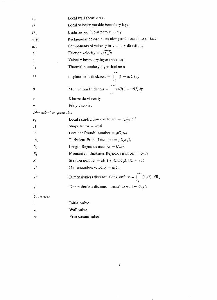
In the earlier paper it was pointed out that Thompson's profile family was inadequate for representing velocities very close to the wall. Thompson assumed that the profiles were linear up to y+ = 8, and at this point there was a discontinuity in velocity gradient. This implied that there was no contribution of eddy conductivity to the heat-transfer process for y+ < 8, and led at the same time to some lack of smoothness in the calculated temperature profiles. Both these effects were greatly enhanced for high Prandtl number fluids where, because of the low laminar conductivity, any contribution from eddy conductivity had a disproportionate effect on the heat transfer.
An improved representation of the blending region was therefore adopted. This is shown in Fig. 1, along with some other proposals, and takes the form
u + = Co + C1 logy + + C2 logZy + + C3 log3 y +,
where the constants are chosen to match sublayer and log-law velocity distributions in slope and magnitude at y+ = 4 and y+ = 30. The general form of this expression was arrived at in the course of work on boundary layers with transpiration (2) where the blending region was required to match sublayer and log laws which varied with transpiration rate. This modification, which for most purposes was quite trivial, enabled continued use to be made of Thompson's profile family which in other respects was entirely adequate.
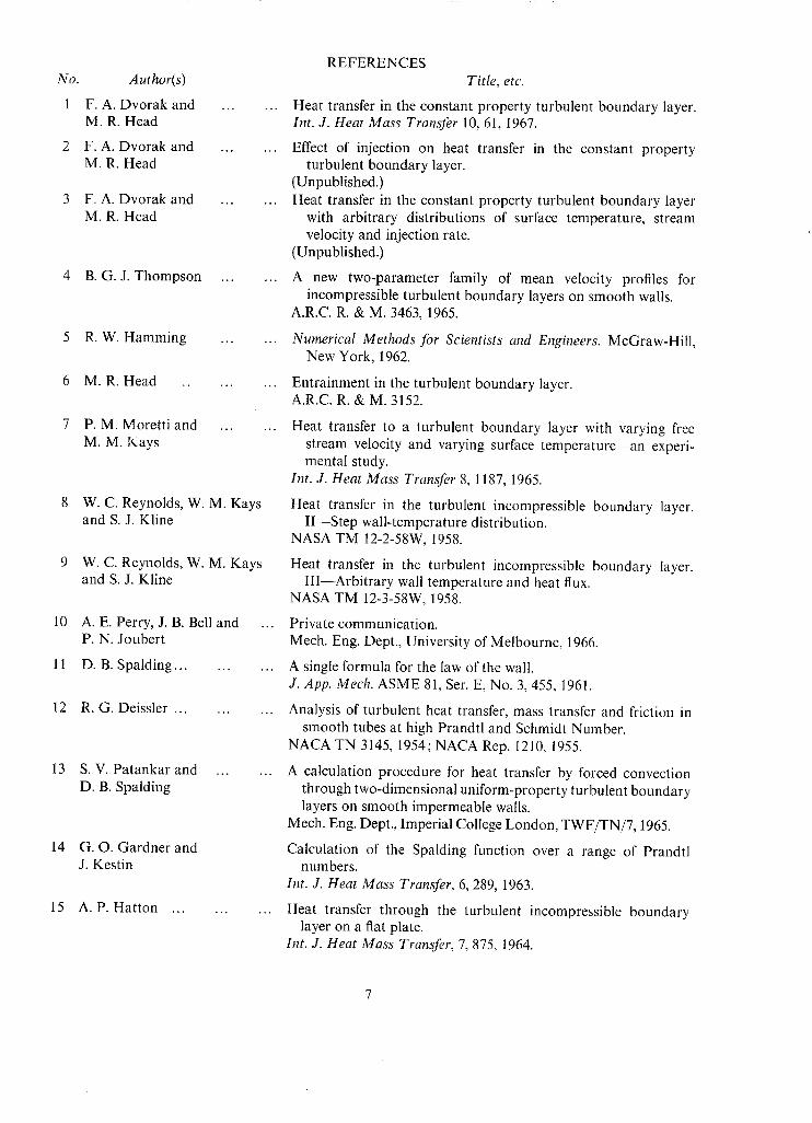
In the calculation of eddy-viscosity profiles, some unsystematic scatter of the calculated points was invariably present. This was initially ignored but it was subsequently found that the smoothness of the calculated temperature profiles was considerably improved if the basic eddy-viscosity (or eddy conductivity) data were subjected to a fairing process. The difficulty was, of course, to smooth the data adequately while leaving overall magnitudes unchanged. With the very close spacing of points in the y-direction that was invariably used, this did not constitute a very serious problem, and the following averaging process (or numerical filter) suggested by Hamming 5 proved satisfactory:
F,, = ( G n_ t + G,, + G.+ 1)/3,
H, = (F,_ 1 + F, + F,+ 0/3.
G, is the original value at y = n and H, is the final smoothed value. A typical result of applying this procedure is shown in Fig. 2.
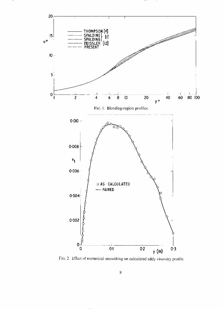
As mentioned in the earlier paper, the simple forward-difference method of Schmidt was used to start the calculation of thermal boundary-layer development. The accuracy of the solution was found to be appreciably influenced by the choice of step size even when the calculation was quite stable. For Pr = I0 it was found necessary to take extremely small intervals in the y-direction (Ay/C = 0"0000125 close to the wall) and correspondingly small increments in x (Ax/C = 0.000025). Halving the intervals in both directions at this stage produced no appreciable change, suggesting that round-off errors were unimportant. The accuracy of the solution was confirmed by checking the incremental heat flux. (See next Section.)
The results of the revised calculations for Pr = 1 and Pr = 10 are shown in Fig. 3 in terms of Stanton number.
4. Checks on Computational Accuracy
The present work has underlined the difficulty of obtaining accurate numerical solutions to the heat-transfer problem, where the effective conductivity may vary by several orders of magnitude in the wall region. Solutions may apparently be regular and well behaved but still appreciably in error. It is therefore important to have available some means of assessing the accuracy of any numerical solution.
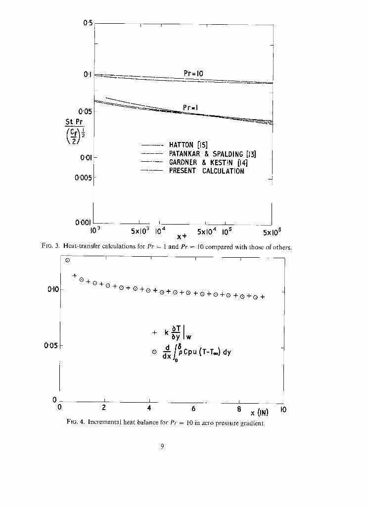
The method of checking mentioned in Ref. 1, of comparing the heat flux in the boundary layer with the heat transferred from the wall up to that position, is useful, but a more sensitive check is to compare the increase of heat flux in the boundary layer over a small interval with that transferred from the wall over the same interval. The results of this check applied to the Pr -- 10 case are shown in Fig. 4.
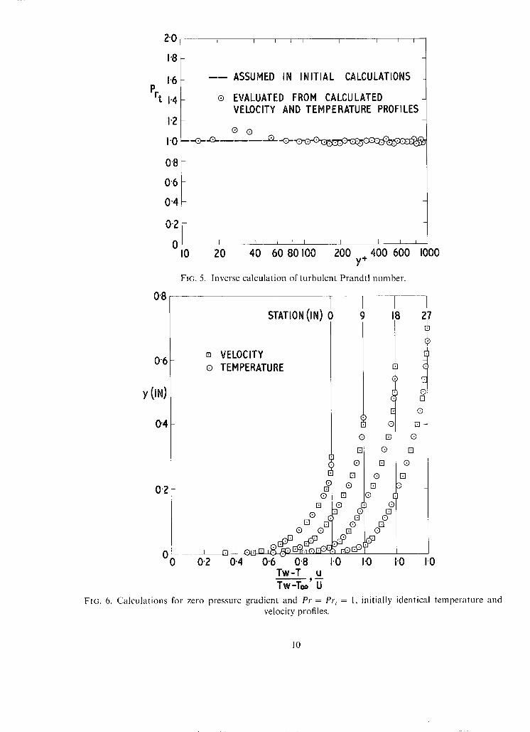
There are two further methods of checking the accuracy of the basic calculation procedure. One is to invert the calculation so that velocity profiles and temperature profiles, obtained from a calculation already performed, are used to determine (for example) the turbulent Prandtl number. If the computations have been accurate throughout, then the appropriate constant value of Pr t used in the original calculation should be recovered. The result of applying this check to a particular case is shown in Fig. 5. A second procedure for checking overall computational accuracy is to perform a calculation for Pr = Prt = 1 and zero pressure gradient. If the temperature profile at some initial station is taken as being identical with the velocity profile at that point, then the application of the full calculation procedure should produce temperature profiles at any distance downstream which are identical with the corresponding velocity
profiles. Fig. 6 shows the result of performing such a calculation, which indicates that, at least for a Prandtl number of unity, the cumulative errors involved in the calculation procedure are small.
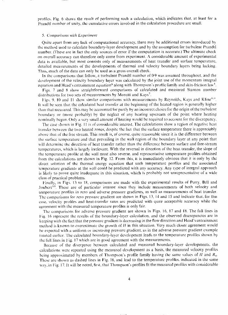
5. Comparisons with Experiment
Quite apart from any lack of computational accuracy, there may be additional errors introduced by the method used to calculate boundary-layer development and by the assumption for turbulent Prandtl number. (These are in fact the only sources of error if the computation is accurate.) The ultimate check oll overall accuracy can therefore only come from experiment. A considerable amount of experimental data is available, but most consists only of measurements of heat transfer and surface temperature, detailed measurements of the developments of thermal and velocity boundary layers being lacking. Thus, much of the data can only be used as a gross overall check.
In the comparisons that follow, a turbulent Prandtl number of 0'9 was assumed throughout, and the development of the velocity boundary layer was calculated by the joint use of the momentum integral equation and Head's entrainment equation ~' along with Thompson's profile family and skin-friction law ¢.
Figs. 7 and 8 show straightforward comparisons of calculated and measured Stanton number distributions for two sets of measurements by Moretti and Kays 7.
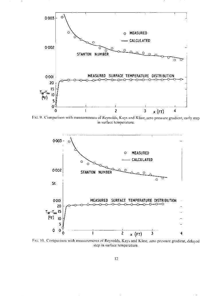
Figs. 9, 10 and 11 show similar comparisons with measurements by Reynolds, Kays and Kline s''~. It will be scen that the calculated heat transfer at the beginning of the heated region is generally higher than that measured. This may be accounted for partly by an incorrect choice for the origin of the turbulent boundary or (more probably) by the neglect of any heating upstream of the point where heating nominally began. Only a very small amount of heating would be required to account for the discrepancy.
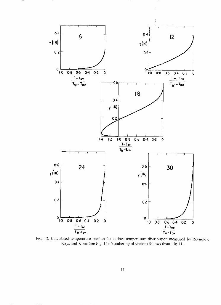
The case shown in Fig. 11 is of considerable interest. The calculations show a region of negative heat transfer between the two heated zones, despite the fact that the surface temperature there is appreciably above that of the free stream. This result is, of course, quite reasonable since it is the difference between the surface temperature and that prevailing in the wall region of the boundary layer at any point that will determine the direction of heat transfer rather than the difference between surface and free-stream temperatures, which is largely irrelevant. With the reversal in direction of the heat transfer, the slope of the temperature profile at the wall must also reverse, and representative temperature profiles obtained from the calculations are shown in Fig. 12. From this, it is immediately obvious that it is only by the direct solution of the thermal energy equation that such temperature profiles and the associated temperature gradients at the wall could be predicted with any accuracy. Any type of integral approach is likely to prove quite inadequate in this situation, which is probably not unrepresentative of a wide class of practical problems.
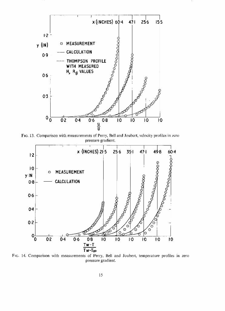
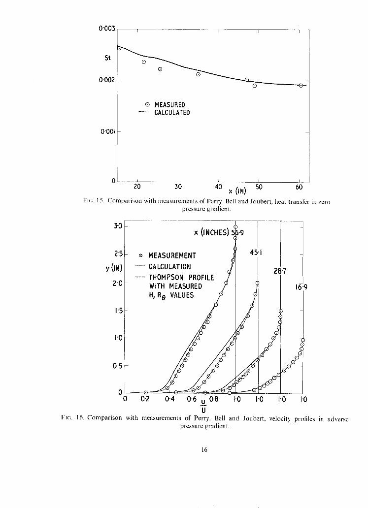
Finally, in Figs. 13 to 18, comparisons are made with the experimental results of Perry, Bell and Joubert l°. These are of particular interest since they include measurements of both velocity and temperature profiles in zero and adverse pressure gradients, as well as measurements of heat transfer. The comparisons for zero pressure gradient are shown in Figs. 13, 14 and 15 and indicate that, for this case, velocity profiles and heat-transfer rates are predicted with quite acceptable accuracy while the agreement with the measured temperature profiles is only fair.
The comparisons for adverse pressure gradient are shown in Figs. 16, 17 and 18. The full lines in Fig. 16 represent the results of the boundary-layer calculation, and the observed discrepancies are in keeping with the fact that the pressure gradient is decreasing in the flow direction and Head's entrainment method is known to overestimate the growth of H in this situation. Very much closer agreement would be expected with a uniform or increasing pressure gradient, as in the adverse pressure gradient example treated earlier. The calculated boundary-layer development leads to the temperature profiles shown by the full lines in Fig. 17 which are in good agreement with the measurements.
Because of the divergence between calculated and measured boundary-layer developments, the calculations were repeated using the measured development as a basis, the measured velocity profiles being approximated by members of Thompson's profile family having the same values of H and R 0. These are shown as dashed lines in Fig. 16, and lead to the temperature profiles, indicated in the same way, in Fig. 17. It will be noted, first, that Thompson's profiles fit the measured profiles with considerable
precision, and second, that the different boundary-layer developments lead to only a very small change in the predicted temperature profiles, which are in good agreement with the measurements.
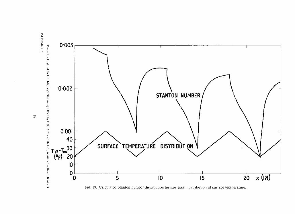
6. A Final Example
Fig. 19 shows the results of a calculation for zero pressure gradient with the saw-tooth temperature distribution indicated on the figure. The Stanton number distribution was somewhat unexpected and was thought to be of sufficient general interest to include here. It will be seen that the streamwise variation of surface temperature has a large effect on the heat transfer, and that there is an effective discontinuity in heat-transfer rate where the gradient of surface temperature changes sign.
7. Conclusions
The following are the conclusions reached from this investigation. (i) The use of precise velocity distributions in the viscous sublayer and blending region is important
for the accurate calculation of heat transfer in fluids of high Prandtl number. (ii) The incremental heat balance provides a necessary check on the accuracy of numerical solutions
of the thermal energy equation. (iii) Useful checks of overall computational accuracy are provided by the inverse calculation of
turbulent Prandtl number and by calculations for Pr t = Pr = 1.
(iv) Calculated and measured heat-transfer rates are in quite fair agreement. The agreement could probably be improved by taking into account the small amount of heating that takes place upstream of the step in temperature in some of the experiments.
(v) Where there are large variations in surface temperature only the direct solution of the heat-transfer equation is likely to yield acceptably accurate results.
(vi) Thompson's velocity-profile family gives an excellent representation of measured velocity profiles. (vii) Small errors in the calculation of the velocity boundary layer have a negligible effect on the
calculated development of the thermal boundary layer. (viii) The streamwise gradient of surface temperature is of considerable importance in determining
heat transfer.
C
Cp
Co,C1,C2,C3 ~ , G ~ , H .
k
k~
q
P
T
LIST OF SYMBOLS
Unheated entry length
Specific heat at constant pressure
Constants in polynomial representing blending region
General functions defined in text
Molecular conductivity
Eddy conductivity
Heat-transfer rate
Density
Temperature
Undisturbed free stream temperature
Local wall temperature
Shear stress
r~ Local wall shear stress
U Local velocity outside boundary layer
U~ Undis turbed free-stream velocity
x, y Rectangular co-ordinates along and normal to surface
u, v Componen t s of velocity in x- and y-directions
U~ Friction velocity = x/%/P
6 Velocity boundary- layer thickness
~r Thermal boundary- layer thickness
fo c~* displacement thickness = (1 - u/U) dy
0 M o m e n t u m thickness = u/U(1 - u/U) dy
v Kinematic viscosity
v t Eddy viscosity
Dimensionless quantities
cf
H
Pr
Prt
Rx
Ro
St
U +
X +
y+
Subscripts
i
W
Local skin-friction coefficient = Zw/½P U 2
Shape factor = 6*/0
Laminar Prandtl number = pCpv/k
Turbulent Prandt l number = pCpvt/k ~
Length Reynolds number = Ux/v
M o m e n t u m thickness Reynolds number = UO/v
Stanton number = k(~T/@)~,/pCpU(Tw - T~)
Dimensionless velocity = u/U~
f? Dimensionless distance along surface = (cl/2)~ dRx
Dimensionless distance normal to wall = U~y/v
Initial value
Wall value
Free-stream value
No. Author(s)
1 F.A. Dvorak and M. R. Head
2 F.A. Dvorak and M. R. Head
3 F.A. Dvorak and M. R. Head
4 B .G . J . Thompson . . . . . .
5 R.W. Hamming ...
6 M.R. Head . . . . .
7 P .M. Moretti and ... M. M. Kays
9
W. C. Reynolds, W. M. Kays and S. J. Kline
W. C. Reynolds, W. M. Kays and S. J. Kline
l0 A.E. Perry, J. B. Bell and P. N. Joubert
11 D.B. Spalding . . . . . .
12 R.G. Deissler . . . . . .
13 S.V. Pa tankarand ... D. B. Spalding
14 G .O. Gardner and J. Kestin
15 A.P. Hatton ...
REFERENCES Title, etc.
... Heat transfer in the constant property turbulent boundary layer. Int. J. Heat Mass Transfer 10, 61, 1967.
... Effect of injection on heat transfer in the constant property turbulent boundary layer.
(Unpublished.) ... Heat transfer in the constant property turbulent boundary layer
with arbitrary distributions of surface temperature, stream velocity and injection rate.
(Unpublished.)
A new two-parameter family of mean velocity profiles for incompressible turbulent boundary layers on smooth walls.
A.R.C.R. & M. 3463, 1965.
... Numerical Methods for Scientists and Engineers. McGraw-Hill, New York, 1962.
... Entrainment in the turbulent boundary layer. A.R.C.R. & M. 3152.
... Heat transfer to a turbulent boundary layer with varying free stream velocity and varying surface temperature--an experi- mental study.
Int. J. Heat Mass Transfer 8, 1187, 1965.
Heat transfer in the turbulent incompressible boundary layer. I I--Step wall-temperature distribution.
NASA TM 12-2-58W, 1958.
Heat transfer in the turbulent incompressible boundary layer. I l l - -Arbi t rary wall temperature and heat flux.
NASA TM 12-3-58W, 1958.
... Private communication. Mech. Eng. Dept., University of Melbourne, 1966.
... A single formula for the law of the wall. J. App. Mech. ASME 81, Ser. E, No. 3, 455, 1961.
... Analysis of turbulent heat transfer, mass transfer and friction in smooth tubes at high Prandtl and Schmidt Number.
NACA TN 3145, 1954; NACA Rep. 1210, 1955.
... A calculation procedure for heat transfer by forced convection through two-dimensional uniform-property turbulent boundary layers on smooth impermeable walls.
Mech. Eng. Dept., Imperial College London, TWF/TN/7, 1965.
Calculation of the Spalding function over a range of Prandtl numbers.
Int. J. Heat Mass Transfer, 6, 289, 1963.
... Heat transfer through the turbulent incompressible boundary layer on a flat plate.
FIG. 4. Incremental heat balance for Pr = l0 in zero pressure gradient.
I0
2"0
1"8
1"6 Prtl.
1"2
0"8
I'0
0"8
0'6
0"4
0'?
0
I I I I I I I I I
- - - - ASSUMED IN INITIAL CALCULATIONS
(3 EVALUATED FROM CALCULATED VELOCITY AND TEMPERATURE PROFILES
(3!) (3 - - -o- -o
i I L 1 I I i I
I0 20 40 60 80 I00 200 400 600 y÷
FIG. 5. Inverse ca lcula t ion of tu rbulen t Prandt l number .
I I I STATION (IN) 0 9 1,8
I
I000
0"6
yON)
[] VELOCITY (3 TEMPERATURE
0'4
0? rq
@ rq
O C
0 ° . . . w . . . . .
0"2 0"4 0"6 0"8 I'0 1t3 I'0 I0 Tw-T u T W - ~ ' U
FIG. 6. Ca lcu la t ions for zero pressure gradient and P r = Pr t = 1, ini t ial ly identical t empera tu re and velocity profiles.
10
0"003
St
0002
0"001
( ~ I I 7-- I
I t I I
02 3 4 s x (~T)
FIG. 7. Comparison with measurements of Moretti and Kays zero pressure gradient, step in surface temperature (Run 1).
0"003
St
0"002
0"001
Q) ~ I I ]
\ o \ o MEASUREMENT
oo ,-, - - CALCULATION
® ®0000 ~ O0000CX~O0 o 0 o
0 I I
2 3 4 5 x (FT} 6
FIG. 8. Comparison with measurements of Moretti and Kays, adverse and favourable pressure gradients, step in surface temperature (Run 33).
I1
I I I 1
c ) ~ c> MEASURED
0 '003-
CALCU LAT ED 0'002 o--.~.,~_ _ ~ _
STANTON NUMBER" ~ c:> ~._...c~:7_...~....~o
0001 MEASURED SURFACE TEMPERATURE DISTRIBUTION 20 15
Tw-Too (OF) 10
5 0 I ~ I I
0 I 2 3 x (FT) 4
Fl(;. 9. Comparison with measurements of Reynolds, Kays and Kline, zero pressure gradient, early step in surface temperature.
0"003
0-002
St
0001
20
Tw-Too 15
(oF) 10
5
0 0
I [ I
c > ~ , c> MEASURED e o~. ~ CALCULATED
STANTON NUMBER o o Q
MEASURED SURFACE TEMPERATURE DISTRIBUTION
I I 3 - . . . . . .
0 I 2 x (FT) 3 4
Fro;. I0. Comparison with measurements of Reynolds, Kays and Kline, zero pressure gradient, delayed step in surface temperature•
12
0"004
0"002
0
-0"002
20 T w -T® (°F) iO
FIG. l 1.
0
12
8
24
r 30 STANTON NUMBER
o MEASURED --CALCULATED
~T-- DISTRIBUTION ~ D SURFACE TEMPERATURE
,
0 I 2 X (FT) 3 z
Comparison with measurements of Reynolds, Kays and Kline, zero pressure gradient, double pulse heat input.
13
0"4
y(IN)
0"2
i I I I
6
I'0 0"8 0'6 0'4 0'2 0
T-Too
T W- Too
06
y( ' " )
0'4
I L I I
?4
0-2
o I'0 0"8 0-6 0"4 0'2 0
T - T~
0'4
y(JN)
0'2
I 0"6 I I
0"4
) / ( I N )
I I I
IZ
0~: I i I I I'0 0"8 0'6 0"4 0"2 0
T - T o o
' T W -Too
I I I I
I-4 1"2 I ' 0 0"8 0 ' 6 0 ' 4 0 -2 0 T-T~
T W -T~, L I I I
o.6 - 3 0
yON)
0"4
0"2 / I'0 0"8 0'6 0'4 0"2 0
T -Too Tw-T~ Tw-T~
FIG. 12. Calculated temperature profiles for surface temperature distribution measured by Reynolds, Kays and Kline (see Fig. l 1). Numbering of stations follows from Fig. I I.
14
J ' I I I I x(INCHES) 60"4 47-1 25"6 15"5
I'?
y (IN)
0"9
0"6
0"3
0 0 0"2 0"4 0"6 0"8 I'0 I'0 I'0 I'0 U U
FIG. 13. Comparison with measurements of Perry, Bell and Joubert, velocity profiles in zero pressure gradient.
' ' ' ' I ~ I I / I x ( INCHES) 21.S 7 5 6 35.1 47.1 4 0 . 8 60 -4