812

Heat Transfer Characteristics of Mixed Electroosmotic and

Pressure Driven Micro-Flows∗

Keisuke HORIUCHI∗∗ and Prashanta DUTTA∗∗∗

We analyze heat transfer characteristics of steady electroosmotic flows with an arbitrarypressure gradient in two-dimensional straight microchannels considering the effects of Jouleheating in electroosmotic pumping. Both the temperature distribution and local Nusselt num-ber are mathematically derived in this study. The thermal analysis takes into considerationof the interaction among advective, diffusive, and Joule heating terms to obtain the thermallydeveloping behavior. Unlike macro-scale pipes, axial conduction in micro-scale cannot benegligible, and the governing energy equation is not separable. Thus, a method that considersan extended Graetz problem is introduced. Analytical results show that the Nusselt numberof pure electrooosmotic flow is higher than that of plane Poiseulle flow. Moreover, when theelectroosmotic flow and pressure driven flow coexist, it is found that adverse pressure gradi-ent to the electroosmotic flow makes the thermal entrance length smaller and the heat transferability stronger than pure electroosmotic flow case.

Key Words: Mixed Electroosmotic and Pressure Driven Flows, Microfluidics, JouleHeating, Extended Graetz Problem

1. Introduction

The emerging lab-on-a-chip micro-fluidic devices aregetting more attention in medical, pharmaceutical, and de-fense applications due to their low-cost, less operationtime, light-weight, and small-size advantages. One ofthe key functionalities of these lab-on-a-chip devices is totransport liquid or reagent from one place to another. Arecent study shows electroosmotic pumping is applicableto working fluids of a wide range of conductivity unlikeothers, and it can develop higher head capacity than othermethods(1).

Since the discovery of the electrokinetic phenomenonby F.F. Reuss in 1809(2), there have been numerous ana-lytical, experimental, and numerical studies on this phe-nomenon. However, so far, most of the studies have beenfocused on the fluid flow behavior under steady(3) – (5) andunsteady(6), (7) electric fields with uniform wall electro-chemical conditions, and not much attention has been paid

∗ Received 14th December, 2005 (No. 05-4275)∗∗ Hitachi Ltd., Mechanical Engineering Research Labora-

tory, 832–2 Horiguchi, Hitachinaka, Ibaraki 312–0034,Japan. E-mail: keisuke.horiuchi.fy@hitachi.com

∗∗∗ School of Mechanical and Materials Engineering, Wash-ington State University, Pullman, WA 99164–2920,U.S.A.

to the thermal behavior.Because the electroosmotic flow is driven in the pres-

ence of a large external electric field, the interaction be-tween the electric field and the charged ions results ina thermal energy generation as Joule heating. In typi-cal electroosmotic flows with a fluid that has an electricalconductivity of 300 µS/m and an applied electric field of100 V/mm(8), the Joule heating contributes 3×106 W/m3.Recently Maynes and Webb have presented thermal be-haviors of fully developed combined pressure and elec-troosmotically driven micro-flows(9). However, their anal-ysis is valid only in the fully developed region.

Analysis of energy equation in the developing regionis particularly challenging for low Reynolds number flows(Re ≤ 100), primarily due to the presence of axial con-duction. This particular problem is known as an extendedGraetz problem, where the associated eigenvalue prob-lem is non-self-adjoint by referring to the standard Sturm-Liouville problem. In literature, none of the previous stud-ies associated with Graetz problem have, until now, dealtwith electroosmotic flow and/or volumetric Joule heating.

For this article, we obtained analytical solutions forthe temperature distributions and heat transfer character-istics of mixed electroosmotic and pressure driven flowsin two-dimensional microchannels. Both developing andfully developed regions have been analyzed for isothermal

Series B, Vol. 49, No. 3, 2006 JSME International Journal

813

channel walls. We have utilized the separation of variablestechnique for homogeneous energy equations introducedby Lahjomri and Oubarra, where they solved the ther-mal problem for arbitrary velocity distribution without anyheat generation(10). Our analysis takes care of the interac-tion among advective, viscous, and Joule heating terms toobtain the temperature distribution within the fluid. Thisanalysis especially identifies the effects of Joule heatingand pressure gradient in microchannels during mixed elec-troosmotic and pressure driven pumping used for design-ing “lab-on-a-chip” micro-fluidic devices.

Nomenclature

cp : specific heat at constant pressure [J/(kg K)]D : half channel height [m]

Ex : streamwise component of electric field [V/m]

1F1 : Kummer confluent hypergeometric function [–]G : normalized heat generation term,

G≡σ(E · E) D2/k(Te−Ts) [–]hξ : local heat transfer coefficient [W/(m2 K)]k : thermal conductivity [W/(m K)]

Nuξ : local Nusselt number, Dhξ/k [–]P : pressure [Pa]

PeT : thermal Peclet number based on the electroos-motic velocity [–]

Rev : ratio of Joule heating to viscous dissipation [–]T : absolute temperature [K]U : non-dimensional streamwise velocity, u/uHS [–]u : streamwise velocity component [m/s]

uHS : Helmholtz-Smoluchowski velocity, −ςεEx/µ

[m/s]x : streamwise coordinate [m]y : cross flow coordinate [m]

Greek Lettersε : permittivity of the medium [C/(V m)]Φ : viscous dissipation [W/m3]η : non-dimensional cross flow coordinate, η = y/D

[–]λn : n-th eigenvalues [–]µ : dynamic viscosity [Pa s]ν : kinematic viscosity [m2/s]θ : non-dimensional temperature, θ ≡ (T −TS )/(Te−

TS ) [–]ρ f : fluid density [kg/m3]σ : electrical conductivity of the buffer fluid [S/m]Ω : non-dimensional pressure gradient, Ω ≡ −D2/

(2µuHS )dP/dx [–]ξ : non-dimensional streamwise coordinate, ξ = x/D

[–]ζ : zeta potential [V]

Subscriptsc : value at the center (y=0)e : value at the inlet (x=0)g : general solution

p : particular solutions : value at the surface (y=D)

2. Mathematical Model

2. 1 Mixed electroosmotic and pressure drivenflows

Analysis of the electroosmotic flow in a two-dimensional microchannel has been presented in a num-ber of studies. The formation of an electric double layer(EDL) on a channel wall is required to have electroosmoticflows. The thickness of an EDL depends on the ion con-centrations. This thickness of EDL typically varies from 1to 10 nm corresponding to the 100 to 1 mM buffer concen-tration. When the thickness of EDL thickness is very thin,the electroosmotic velocity is approximated as Helmholtz-Smoluchowski velocity, uHS

(11), (12), which is a function ofthe zeta potential, ς, the permittivity of the medium, ε, theviscosity of the fluid, µ, and the applied electric field inthe streamwise direction, Ex. Although the electrokineticflow is desired in many bioanalytical applications, theremay be a pressure variation along the channel due to thefollowing reasons:• presence of an alternative pumping mechanism,• placement of a mechanical valve in the flow path,• head difference between the inlet and exit reser-

voirs.The resulting pressure gradient distorts the plug-like ve-locity distribution (Fig. 1). In the absence of an inertialterm due to a low Reynolds number (Re), the momen-tum equation becomes linear. Therefore, the steady ve-locity distribution for the mixed electroosmotic and pres-

Fig. 1 Schematic of mixed electroosmotic and pressure drivenflows: (a) adverse pressure gradient and (b) favorablepressure gradient. Under the ideal conditions of uniformzeta potential and electrolyte concentration, we canobtain pure electroosmotically driven plug flows if thereis no pressure gradient

JSME International Journal Series B, Vol. 49, No. 3, 2006

814

sure driven flow in a two-dimensional straight channel canbe obtained by considering the linear superposition of theelectroosmotic velocity (uHS ) and the plane Poiseulle flowvelocity (uPois)(5) as

u(x,y)=uHS +uPois =−ςεEx

µ− D2

2µdPdx

1−

(y

D

)2,

(1)

where P is the pressure and D is the half channel height.2. 2 Energy transport in mixed electroosmotic-

pressure driven flowsThe governing equation for the two-dimensional

steady thermal energy transport can be presented as

ρ f cPu∂T∂x=∂T∂x

(k∂T∂x

)+∂T∂y

(k∂T∂y

)+Φ+σE2

x , (2)

where ρ f is the fluid density, cP is the specific heat, Tis the absolute temperature, k is the thermal conductiv-ity, Φ≈ µ(∂u/∂y)2 is the viscous dissipation, and σ is theelectrical conductivity of the buffer fluid. The last term,the specific term for electroosmotic flows, is called Jouleheating simply because of the existence of an electric field.Since we have modeled the electrokinetic component ofthe flow velocity with the Helmholtz-Smoluchowski slipvelocity, the viscous dissipation term is mainly due to thepressure driven component of the velocity. Here we as-sume that the flow is hydraulically fully developed fromthe very beginning of the channel, but the temperaturefield is developing. This can be justified for fluid whoseReynolds number is less than one (typical in microflu-idics) and the Prandtl number is greater than one (suchas de-ionized water with a Pr = 7), respectively. There-fore, for the hydraulically fully developed mixed elec-troosmotic and pressure driven flow in a two-dimensionalstraight channel, the ratio of Joule heating to the viscousdissipation can be expressed as,

Rev=

∫ +D

−DσE2

xdy

∫ +D

−Dµ(y/µ dP/dx)2dy

≈ 34µσ

(DΩες

)2

, (3)

where Ω is the normalized pressure gradient (Ω ≡−1/2 dP∗/dξ) and P∗ is the non-dimensional pressure(P∗ ≡PD/(µuHS )). From Eq. (3), it is clear that the ratio ofthe generation terms, Rev, is independent of the externallyapplied electric field, but depends on the characteristic di-mensions, pressure gradient, zeta potential, and electricconductivity. For the flow and electrokinetic parameterranges considered for this study, the same as in our previ-ous work, the above ratio varies between 10 and 10 000.Therefore, we neglected the viscous dissipation term forthis analysis.

For the isothermal surface case, the two-dimensionalenergy equation is subjected to the following boundaryconditions.

T =Te at x=0, 0≤y≤D (4.a)

T <∞ at x→∞, 0≤y≤D (4.b)∂T∂y=0 at 0≤ x<∞, y=0 (4.c)

T =TS at 0≤ x<∞, y=D (4.d)

2. 3 Normalization schemeWe normalize streamwise and cross-stream coordi-

nates (x, y) with the half channel height D (ξ = x/D,η = y/D). Here, D is used as the characteristic lengthas opposed to the hydraulic diameter, DH = 4D. There-fore, the flow Reynolds and Nusselt numbers in this studywill be one fourth of their conventional values, wherethose numbers are calculated based on hydraulic diame-ters. For convenience, we normalize the flow velocity withthe Helmholtz-Smoluchowski velocity, U =u/uHS . Underthis normalization scheme, the non-dimensional stream-wise velocity is

U =u/uHS =1+Ω(1−η2), (5)

where Ω is the non-dimensional pressure gradient. Know-ing the inlet temperature, Te, and the surface tempera-ture, TS , we now define the normalized temperature asθ ≡ (T − TS )/(Te − TS ) and the normalized heat genera-tion term as G ≡ σ(E · E)D2/k(Te −Ts). Based on theabove normalization scheme, the energy equation and cor-responding boundary conditions can be written as fol-lows:

PeT U∂θ

∂ξ=∂2θ

∂ξ2+∂2θ

∂η2+G, (6.a)

θ=1 at ξ=0, 0≤η≤1, (6.b)

θ<∞ at ξ→∞, 0≤η≤1, (6.c)∂θ

∂η=0 at 0≤ ξ <∞, η=0, and (6.d)

θ=0 at 0≤ ξ <∞, η=1, (6.e)

where PeT is the thermal Peclet number for pure electroos-motic flow, and it can be found by multiplying the flowReynolds number based on Helmholtz-Smoluchowski ve-locity with the fluid Prandtl number as PeT = uHS D/α,where α is the thermal diffusivity. The normalized sourceterm, G, represents a ratio of the energy generation to thethermal conduction. An aqueous solution (with a Tris-EDTA buffer) of conductivity, σ=90 µS/cm(7), and an ap-plied electric field of 400 V/mm, will contribute to G = 1in a 100-µm thick microchannel for Te − TS = 5 K. Inthe above normalization process, the temperature indepen-dence of the fluid properties is assumed. Although thefluid viscosity, µ, and thermal conductivity, k, are strongfunctions of the fluid temperature, their variations can beneglected for a temperature difference of 10 K or smaller.Moreover, both the electric field, E= (Ex,0), and the elec-trical conductivity, σ, are assumed uniform throughout thechannel. The normalized energy equation presented byEq. (6.a) is a second order partial differential equation.

Series B, Vol. 49, No. 3, 2006 JSME International Journal

815

3. Analysis of Normalized Energy Equation

Let’s decompose the normalized temperature, θ, intotwo parts,

θ= θP+θg, (7)

where θP is chosen so that θg satisfies a homogeneousequation. Now, we seek a particular solution θP as a func-tion of an η subject to the boundary conditions, Eqs. (6.d)and (6.e). We obtain a solution for a particular type offunction:

θP=G2

(1−η2). (8)

On the other hand, the governing equation for θg becomeshomogeneous. Suppose the solution to the homogeneousproblem has the following form (for details see Ref. (11)):

θg=∞∑

n=1An fn(η)exp

[− λ

2n

PeTξ

], (9)

where An are the coefficients, fn are the eigenfunctions,and λn are the eigenvalues. By substituting Eqs. (7) and (9)into Eq. (6), we obtain the following nonlinear eigenvalueproblem:

d2 fndη2+λ2

n

(λn

PeT

)2

+U

fn=0, (10.a)

d fndη=0 at η=0, and (10.b)

fn=0 at η=1 (10.c)

The solution to Eq. (10.a) under a symmetric boundarycondition, Eq. (10.b), can be expressed as

fn= exp

[−1

2λn

√Ωη2

]1F1(a;b;z), (11.a)

where 1F1(a;b;z) =∞∑j=0

((a) j/(b) j)(zj/ j!) is the Kummer

confluent hypergeometric function, (a) j and (b) j areknown as the Pochhammer symbols, and the variable ofthe hypergeometric function in this particular study is

a=−λ3

n−Pe2T (λn(1+Ω)− √Ω)

4√ΩPe2

T

, (11.b)

b=1/2, and (11.c)

z=λnη2√Ω. (11.d)

The eigenfunctions fn presented by Eq. (11.a) have a se-quence of eigenvalues λn, and fn∞n=1 forms a base forthe function space L2(0,1). Our next goal is to findthe eigenvalues λn from Eq. (11.a) by utilizing the wallboundary condition given in Eq. (10.c). For this nonlin-ear eigenvalue problem, the Secant method is utilized tofind out the corresponding eigenvalues, and they are pre-sented in Table 1. Note that the eigenfunctions fn are notmutually orthogonal (by referring to the standard Sturm-Liouville problem) since the eigenvalues λn occur non-linearly in Eq. (10.a). We use the Gram-Schmidt orthogo-nal procedure in order to determine the coefficients, An,

Table 1 First ten terms of coefficients (An) and correspondingeigenvalues (λn) for PeT =1

from a set of linearly independent eigenfunctions fn∞n=1.Therefore, the normalized temperature distribution can beobtained from Eqs. (7) – (9) as

θ= θp+θg=G2

(1−η2)+∞∑

n=1An fn exp

[− λ

2n

PeTξ

]. (12)

It is important to note that the normalized temperature dis-tribution obtained in Eq. (12) is valid for Ω > −1.5. Ifthe normalized pressure gradient were less than −1.5, thenet flow would change direction, which is undesirable forthe presented mathematical model. The correspondingNusselt number for the mixed electroosmotic and pres-sure driven flow can be obtained by normalizing the heattransfer coefficient based on the Newton’s Law of Cooling(hξ = (−k∂T/∂y)y=D/(Ts−Tm)= (k/D)(−∂θ/∂η)η=1/θm).

Nuξ =Dhξ

k

=

5(3+2Ω)

(G−

∞∑n=1

An exp

[− λ

2n

PeTξ

]∂ fn∂η

∣∣∣∣∣η=1

)

G(5+4Ω)+15∞∑

n=1An exp

[− λ

2n

PeTξ

]∫ 1

0U fndη

.

(13)

4. Discussion of Results

For mixed electroosmotic and pressure driven flows,the analytical solutions of the heat transfer characteristicsare obtained with Eqs. (12) and (13). The convergence ofthe infinite series is very slow at ξ = 0, and therefore, wehave plotted our results from ξ=0.01. The analytical solu-tions presented here are for Re<1, Pr>1, and D≥1 000λwhere λ is the Debye length. Therefore, the hydrodynamicentry length is negligible, and the mixed velocity distribu-tion is justified from the very beginning of the channel. Onthe other hand, the thermally developing region can existwhile hydraulically fully developed.

JSME International Journal Series B, Vol. 49, No. 3, 2006

816

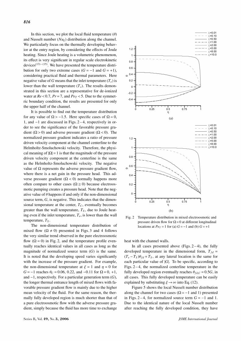
In this section, we plot the local fluid temperature (θ)and Nusselt number (Nuξ) distribution along the channel.We particularly focus on the thermally developing behav-ior at the entry region, by considering the effects of Jouleheating. Since Joule heating is a volumetric phenomenon,its effect is very significant in regular scale electrokineticdevices(13) – (15). We have presented the temperature distri-bution for only two extreme cases (G = −1 and G = +1),considering practical fluid and thermal parameters. Herenegative value of G means that the inlet temperature (Te) islower than the wall temperature (Ts). The results demon-strated in this section are a representative for de-ionizedwater at Re<0.7, Pr=7, and PeT <5. Due to the symmet-ric boundary condition, the results are presented for onlythe upper half of the channel.

It is possible to find out the temperature distributionfor any value of Ω > −1.5. Here specific cases of Ω = 0,1, and −1 are discussed in Figs. 2 – 4, respectively in or-der to see the significance of the favorable pressure gra-dient (Ω > 0) and adverse pressure gradient (Ω < 0). Thenormalized pressure gradient indicates a ratio of pressuredriven velocity component at the channel centerline to theHelmholtz-Smoluchowski velocity. Therefore, the physi-cal meaning of |Ω|=1 is that the magnitude of the pressuredriven velocity component at the centerline is the sameas the Helmholtz-Smoluchowski velocity. The negativevalue of Ω represents the adverse pressure gradient flow,where there is a net gain in the pressure head. This ad-verse pressure gradient (Ω < 0) normally happens moreoften compare to other cases (Ω ≥ 0) because electroos-motic pumping creates a pressure head. Note that the neg-ative value of θ happens if and only if the non-dimensionalsource term, G, is negative. This indicates that the dimen-sional temperature at the center, TC , eventually becomesgreater than the wall temperature, TS , due to Joule heat-ing even if the inlet temperature, Te, is lower than the walltemperature, TS .

The non-dimensional temperature distribution ofmixed flow (Ω 0) presented in Figs. 3 and 4 followsthe very similar trend observed in the pure electroosmoticflow (Ω = 0) in Fig. 2, and the temperature profile even-tually reaches identical values in all cases as long as themagnitude of normalized source term (G) is the same.It is noted that the developing speed varies significantlywith the increase of the pressure gradient. For example,the non-dimensional temperature at ξ = 1 and η = 0 forG =−1 reaches θC = 0.06, 0.22, and −0.11 for Ω= 0, +1,and −1, respectively. For a particular generation term (G),the longer thermal entrance length of mixed flows with fa-vorable pressure gradient flow is mainly due to the highermean velocity of the fluid. For the same reason, the ther-mally fully developed region is much shorter than that ofa pure electroosmotic flow with the adverse pressure gra-dient, simply because the fluid has more time to exchange

(a)

(b)

Fig. 2 Temperature distribution in mixed electroosmotic andpressure driven flow for Ω=0 at different longitudinallocations at PeT =1 for (a) G=−1 and (b) G=+1

heat with the channel walls.In all cases presented above (Figs. 2 – 4), the fully

developed temperature in the dimensional form, T f d =

(Te −TS )θ f d +TS , at any lateral location is the same foreach particular value of |G|. To be specific, according toFigs. 2 – 4, the normalized centerline temperature in thefully developed region eventually reaches θ f d,C = 0.5G, inall cases. This fully developed temperature can be easilyexplained by substituting ξ→∞ into Eq. (12).

Figure 5 shows the local Nusselt number distributionalong the channel for two cases (Ω=−1 and 1) presentedin Figs. 2 – 4, for normalized source term G = −1 and 1.Due to the identical nature of the local Nusselt numberafter reaching the fully developed condition, they have

Series B, Vol. 49, No. 3, 2006 JSME International Journal

817

(a)

(b)

Fig. 3 Temperature distribution in mixed electroosmotic andpressure driven flow for Ω=+1 at different longitudinallocations at PeT =1 for (a) G=−1 and (b) G=+1

been presented up to ξ = 100. The local Nusselt numberabruptly decays to reach a flat value within twenty char-acteristic lengths (ξ = 20 or x = 20D). The rationale forthis abrupt decay is that a thermal boundary layer devel-ops along the direction of the flow. The spike in the lo-cal Nusselt number distribution for G = −1 indicates thelocation along the channel where the mean temperatureapproaches the surface temperature. For negative normal-ized generation (G<0), the fluid temperature (T ) increasesdue to both the Joule heating and the surface thermal con-dition, until it exceeds the surface temperature. It is clearthat the fully developed Nusselt number approaches thesame value as long as the magnitude of G is identical. Forpositive normalized generation (G> 0), the fluid tempera-

(a)

(b)

Fig. 4 Temperature distribution in mixed electroosmotic andpressure driven flow for Ω=−1 at different longitudinallocations at PeT =1 for (a) G=−1 and (b) G=+1

ture (T ) decreases constantly in order to satisfy the lowerwall surface temperature boundary, whereas heat genera-tion exists inside the channel. It turns out that the entrancelength is the same for the same absolute value of normal-ized heat generation, G, due to energy balance betweenthe amount of heat generation and heat rejection, whilethe entrance length gets longer as the pressure gradient isincreased.

For each case, we also studied the dependence ofthe thermal Peclet number based on the Helmholtz-Smoluchowski velocity. For a particular flow, the fullydeveloped Nusselt number is independent of the Pecletnumber, and it does not depend on the magnitude of thesource term. The fully developed Nusselt numbers for dif-

JSME International Journal Series B, Vol. 49, No. 3, 2006

818

(a)

(b)

Fig. 5 Local Nusselt number distribution along channel fordifferent Joule heating values at different Peclet numbersfor (a) Ω=−1 and (b) Ω=+1

ferent source terms are presented in Table 2. Here, ourNusselt number values are computed based on their hy-draulic diameter (NuDH = 4NuD). For both positive andnegative source terms with the same magnitudes consid-ered in this study (G = −1 and 1), the Nusselt numberin the fully developed region becomes the same. In pureelectroosmotic flow, the Nusselt number reaches a valueof 12.0 in the fully developed region, which agrees withother researchers(16). For cases without Joule heating theheat transfer characteristics of pure electroosmotic floware identical to the classical isothermal heat transfer in aslug flow, which the fully developed Nusselt number is9.868(17). In the fully developed region, the Nusselt num-ber for the electroosmotic flow is significantly higher than

Table 2 Comparison of Nusselt numbers based on hydraulicdiameter (NuDH ) in fully developed region comparedwith existing literature

that of the Poiseuille flow. The higher heat transfer char-acteristics in a pure electroosmotic flow can be attributedto the plug-like uniform velocity. In pure Poiseuille flows,the fully developed Nusselt number also compares withthat in existing literature(10) for identical geometric condi-tions. In the fully developed region our analytical resultsexactly match the other existing studies. Note that the heatflux at the wall is the same for all cases in the fully devel-oped region, and it can be explained by the temperaturedistribution in Figs. 2 – 4. This implies that the normalizedbulk mean temperature gets higher as the pressure gradi-ent increases, which solely depends on the normalized ve-locity distribution across the channel. In other words, ahigher flow rate leads to less heat transfer.

5. Conclusions

We obtained analytical solutions for the heat transfercharacteristics of mixed electroosmotic-pressure drivenflows in two-dimensional straight microchannels for con-stant zeta potentials, buffer concentrations, and externalelectric fields. This analysis takes care of the interac-tion among advective, viscous, and Joule heating terms toobtain the temperature distribution within the fluid. Ouranalysis resulted in the following:

1. For an isothermal channel surface condition beforeit reaches an identical profile, the local fluid temperature indimensional form (T ) decreases for a positive source term(G > 0) and increases for a negative source term (G < 0)along the channel.

2. For a particular flow type (in the fully developedregion), the normalized heat transfer coefficient reachesthe same value for both the positive and negative sourceterms.

3. The Nusselt number of the mixed electroosmoticand pressure driven flow is smaller than that of the pureelectroosmotic flow for favorable pressure gradients.

4. Electroosmotic flow with adverse pressure gradi-ent provides the best heat transfer performance.

5. The temperature profile in the fully developed re-gion is independent of the Peclet number and pressure gra-dient.

Series B, Vol. 49, No. 3, 2006 JSME International Journal

819

6. In the mixed electroosmotic-pressure driven flows,the thermal entrance length increases with the imposedpressure gradient.

7. The entrance length is the same for the same mag-nitude of normalized heat generation, G.

Acknowledgements

This work has been partially funded by WashingtonState University Office of Research and partially by theNational Science Foundation (CTS 0300802). The authorswould like to thank Prof. Hong-Ming Yin for his valuablesuggestions.

References

( 1 ) Chen, C.H. and Santiago, J.G., A Planar Electroos-motic Micropump, J. Microelectromechanical Sys-tems, Vol.11 (2002), pp.672–683.

( 2 ) Reuss, F.F., Charge-Induced Flow, Proceedings ofthe Imperial Society of Naturalists of Moscow, Vol.3(1809), pp.327–344.

( 3 ) Burgreen, D. and Nakache, F.R., Electrokinetic Flow inUltrafine Capillary Silts, J. Physical Chemistry, Vol.68(1964), pp.1084–1091.

( 4 ) Rice, C.L. and Whitehead, R., Electrokinetic Flow ina Narrow Cylindrical Capillary, J. Physical Chemistry,Vol.69 (1965), pp.4017–4024.

( 5 ) Dutta, P. and Beskok, A., Analytical Solution of Com-bined Electroosmotic/Pressure Driven Flows in Two-Dimensional Straight Channels: Finite Debye LayerEffects, Analytical Chemistry, Vol.73 (2001), pp.1979–1986.

( 6 ) Soderman, O. and Jonsson, B., Electro-Osmosis: Ve-locity Profiles in Different Geometries with Both Tem-poral and Spatial Resolution, J. Chern. Phys., Vol.105(1996), pp.10300–10311.

( 7 ) Wong, P.K., Chen, C.Y., Wang, T.H. and Ho, C.M.,An AC Electroosmotic Processor for Biomolecules,Proc. of 12th International Conference on Solid StateSensors, Actuators and Microsystems, Vol.1 (2003),pp.20–23.

( 8 ) Zeng, S., Chen, C.H., Mikkelsen, J.C., Jr. and Santiago,J.G., Fabrication and Characterization of Electroos-motic Micropumps, Sensors and Actuators B, Vol.79(2001), pp.107–114.

( 9 ) Maynes, D. and Webb, B.W., Fully-Developed Ther-mal Transport in Combined Pressure and Electro-Osmotically Driven Flow in Microchannels, ASME J.Heat Transfer, Vol.125 (2003), pp.889–895.

(10) Lahjomri, J. and Oubarra, A., Analytical Solution ofthe Graetz Problem with Axial Conduction, ASME J.Heat Transfer, Vol.121 (1999), pp.1078–1083.

(11) Hunter, R.J., Zeta Potential in Colloid Science: Prin-ciples and Applications, First ed., (1981), AcademicPress Inc, New York.

(12) Probstein, R.F., Physiochemical Hydrodynamics, Sec-ond ed., (1994), Wiley and Sons Inc., New York.

(13) Arfken, G., Mathematical Methods for Physicists,Third ed., (1985), Academic Press, Florida.

(14) Gobie, W.A. and Ivory, C.F., Thermal Model of Cap-illary Electrophoresis and a Method of Counteract-ing Thermal Band Broadening, J. Chromatography,Vol.516 (1990), pp.191–210.

(15) Burgi, D.S., Salomon, K. and Chien, R.L., Methodsfor Calculating the Internal Temperature of CapillaryColumns during Capillary Electrophoresis, J. LiquidChromatography, Vol.14 (1991), pp.847–867.

(16) Maynes, D. and Webb, B.W., Fully Developed Electro-Osmotic Heat Transfer in Microchannels, Int. J. Heatand Mass Transfer, Vol.46 (2003), pp.1359–1369.

(17) Burmeister, L.C., Convective Heat Transfer, Seconded., (1993), Wiley and Sons, New York.

JSME International Journal Series B, Vol. 49, No. 3, 2006