Accepted Manuscript

HEAT transfer modelling IN exhaust systems OF high-performance two-strokeengines

JoséManuel Luján, Héctor Climent, Pablo Olmeda, Víctor Daniel Jiménez

PII: S1359-4311(14)00309-3

DOI: 10.1016/j.applthermaleng.2014.04.045

Reference: ATE 5569

To appear in: Applied Thermal Engineering

Received Date: 18 November 2013

Revised Date: 10 March 2014

Accepted Date: 19 April 2014

Please cite this article as: J. Luján, H. Climent, P. Olmeda, V.D. Jiménez, HEAT transfer modelling INexhaust systems OF high-performance two-stroke engines, Applied Thermal Engineering (2014), doi:10.1016/j.applthermaleng.2014.04.045.

This is a PDF file of an unedited manuscript that has been accepted for publication. As a service toour customers we are providing this early version of the manuscript. The manuscript will undergocopyediting, typesetting, and review of the resulting proof before it is published in its final form. Pleasenote that during the production process errors may be discovered which could affect the content, and alllegal disclaimers that apply to the journal pertain.

MANUSCRIP

T

ACCEPTED

ACCEPTED MANUSCRIPT

HEAT TRANSFER MODELLING IN EXHAUST SYSTEMS OF

HIGH-PERFORMANCE TWO-STROKE ENGINES

JoséManuel Luján, Héctor Climent*, Pablo Olmeda, Víctor Daniel Jiménez

CMT Motores Térmicos, Universitat Politècnica de València, Spain

* Corresponding author. Postal address: CMT Motores Térmicos, 2º Edificio de Investigación.

Universitat Politècnica de València. Camino de Vera s/n. 46022. Valencia. Spain.

ABSTRACT

Heat transfer from the hot gases to the wall in exhaust systems of high-performance two-stroke

engines is underestimated using steady state with fully developed flow empirical correlations.

This fact is detected when comparing measured and modelled pressure pulses in different

positions in the exhaust system. This can be explained taking into account that classical

expressions have been validated for fully developed flows, a situation that is far from the flow

behaviour in reciprocating internal combustion engines. Several researches have solved this

phenomenon in four-stroke engines, suggesting that the unsteady flow is strongly linked to the

heat transfer. This research evaluates the correlations proposed by other authors in four stroke

engines and introduces a new heat transfer model for exhaust systems in two-stroke, high

performance, gasoline engines. The model, which accounts for both the entrance length effect

and flow velocity fluctuations, is validated against experimental measurements. Comparisons of

the proposed model with other models are performed, showing not negligible differences in the

scavenge process related parameters.

Keywords: heat transfer, unsteady flow, 1D modelling, two-stroke engine

1. INTRODUCCION

In comparison with four-stroke engines, the wave propagation phenomena inside the exhaust

system in two-stroke engines is even more critical because of its influence in the cylinder

scavenging process, which determines the residual gases and trapped mass for the next engine

cycle. The instantaneous pressure in the exhaust system depends basically on the in-cylinder

thermodynamic conditions, the opening speed of the exhaust port, the geometry of the exhaust

MANUSCRIP

T

ACCEPTED

ACCEPTED MANUSCRIPTsystem and the heat transfer through the exhaust system [1]. Thus, heat transfer modelling in

exhaust systems is an important issue if accurate engine simulations are desired. The use of

conventional models to reproduce the heat transfer loss from the hot gases to the wall in

exhaust systems of high-performance two stroke engines usually leads to underestimate the

phenomenon.

This is shown in the wave propagation delays between the modelled and measured

instantaneous exhaust pressure pulses as Fig. 1 depicts. These results are obtained in a 125 cc

two-stroke engine at 12500 rpm and full load. The cylinder blow-down is observed, in both

measured and calculated pressure traces, by a rapid increase in the exhaust pressure when the

exhaust port is opened (at 100 crank angle degree). This pressure pulse travels through the

exhaust system at the local sound speed, which depends on the gas temperature and, hence,

the heat transfer to the walls. It is observed that the pressure pulses originated by the exhaust

system geometry travel faster in the calculated instantaneous pressure when using the Dittus-

Boelter correlation [2] for the estimation of the convection heat coefficient.

For the heat transfer modelling in reciprocating internal combustion engines, correlations for

fully developed turbulent flow, type Nu = f (Re, Pr), are used. Among them, the classic

expressions developed by Dittus-Boelter [2], Sieder-Tate [3] and Huber [4] are the most used.

Several researchers modelled the heat transfer in exhaust manifolds and pipes based on

classical expressions but re-calibrating their parameters [5-8].

However, in unsteady processes, those correlations are improved with dimensionless

coefficients to calculate the heat transfer in straight exhaust manifolds in four-stroke engines.

This phenomenon is modelled taking account: (i) the entrance effects of the flow blown from the

cylinder together with the development of the turbulence along the pipes [9-13], and (ii) the

highly unsteady flow with rapid velocity variations, which are not negligible [14].

The main objectives of this research are: first the evaluation and applicability of general

empirical heat transfer models in exhaust systems for high-performance two stroke engines

and, the introduction of a new heat transfer model more suitable for these engines . The

proposed model, which is added to a 1D engine simulation code, takes into account the

entrance phenomena and the highly unsteady flow inside the exhaust system. In order to verify

that the wave phenomena are reproduced with good accuracy, the instantaneous pressure

MANUSCRIP

T

ACCEPTED

ACCEPTED MANUSCRIPTtraces in different parts of the exhaust system and the gases mass flow through the engine are

compared. In a next step, the engine model can be used to obtain and analyze the scavenging

coefficients. Thus, the thermo-and fluid dynamic variables that characterize the engine

performance are calculated.

The paper is structured as follows. First, in section 2, the one-dimensional engine model and

the development of the proposed heat transfer model are presented. Then, in section 3, the

experimental methodology that will be used to calibrate and validate the proposed model is

described. After that, the calibration parameters that define the explored models are shown in

section 4. The results of the evaluation and validation of heat transfer model proposed is the

subject of section 5. Moreover, in this section, the results obtained are contrasted with

experimental measurements and compared with other models found in the literature. Finally, the

main conclusions of this research are presented.

2. MODEL DEVELOPMENT

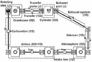
2.1 1D engine model

Wave propagation phenomena during gas exchange processes inside internal combustion

engines are assumed to be one dimensional. In the case under consideration, a wave action

model, which solves the unsteady, non linear and one dimensional flow equations using a finite

difference scheme [15], is used to model the high performance two stroke engine.

Fig. 2 shows a schematic layout of the 125 cc engine. As depicted in this figure, it is observed

that the engine is composed basically of three kinds of elements: ducts (1D), volumes (0D) and

junctions (J). Volumes (such as cylinder, crankcase, airbox and atmosphere) are calculated

using a zero dimensional approach, by solving mass and energy conservation equations.

In−cylinder heat release rate for combustion simulation is obtained by means of correlations for

Wiebe function parameters [16].

Effective area of junctions (such as exhaust and transfer ports, rotating disk or reed valves)

between ducts and volumes are solved by means of a discharge coefficient, which has to be

previously obtained in a steady flow bench. Boundary conditions are solved using the method of

characteristics and then coupled with the finite difference calculation in the ducts [17]. Exhaust

MANUSCRIP

T

ACCEPTED

ACCEPTED MANUSCRIPTsystems, silencer and airbox were characterized in an impulse test rig [18]; subsequently they

were simulated individually with the 1D code, for later setup of the complete geometry.

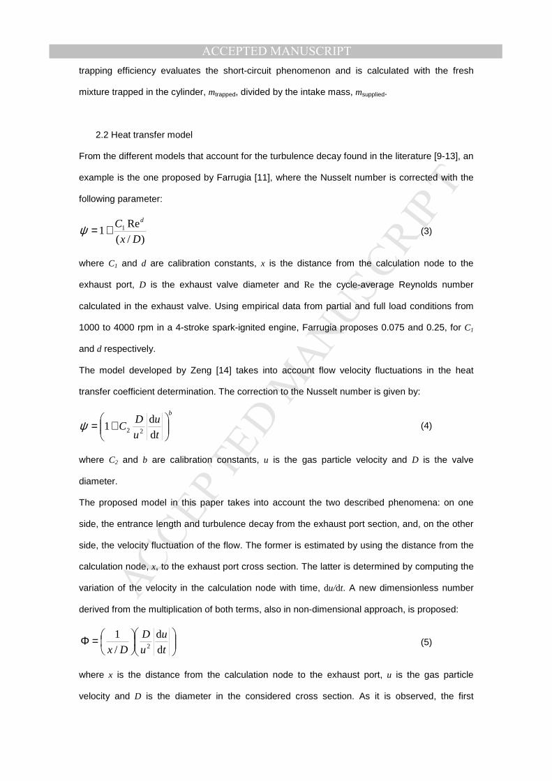
The governing equations that describe the one dimensional non homentropic gas flow, with the

consideration of transversal section change, friction and heat transfer in a pipe, form a non

homogenous hyperbolic system, and are represented in vector notation as Daneshyar [19]:

∂ ∂+ + + =∂ ∂ 1 2 0t x

W FC C (1)

This conservation law system, comprising the continuity, momentum and energy equations, is

complemented by the equation of state or the real gas properties [20]. In Eq. (1), W is the

desired state vector of the solution, F is the flux vector and C the source term separating the

effect of the area changes from the effect of friction and heat transfer. The one dimensional gas

flow governing equations was traditionally arranged in the vector form shown in Eq. (2):

( )

( ) ( )

ρρρρ

γρργγ

ρρ

ργρ ρ

γ

+ = =

++ −−

= = + − −

2

22

2

1 22

, ( )

2 12 1

01

,

2 1

u

u pux t

u pu pu

u

u dSx g

S dxu pu q

W F W

C W C W

(2)

This set of equations is solved by using the TVD method [21], which is programmed in the

computer code together with the boundary conditions.

The scavenge process inside the cylinder is an important issue in two−stroke engines. A

well−known model [22] to account for short circuit phenomenon was used in the present study.

This type of models allow the estimation of scavenge related parameters, such as: delivery

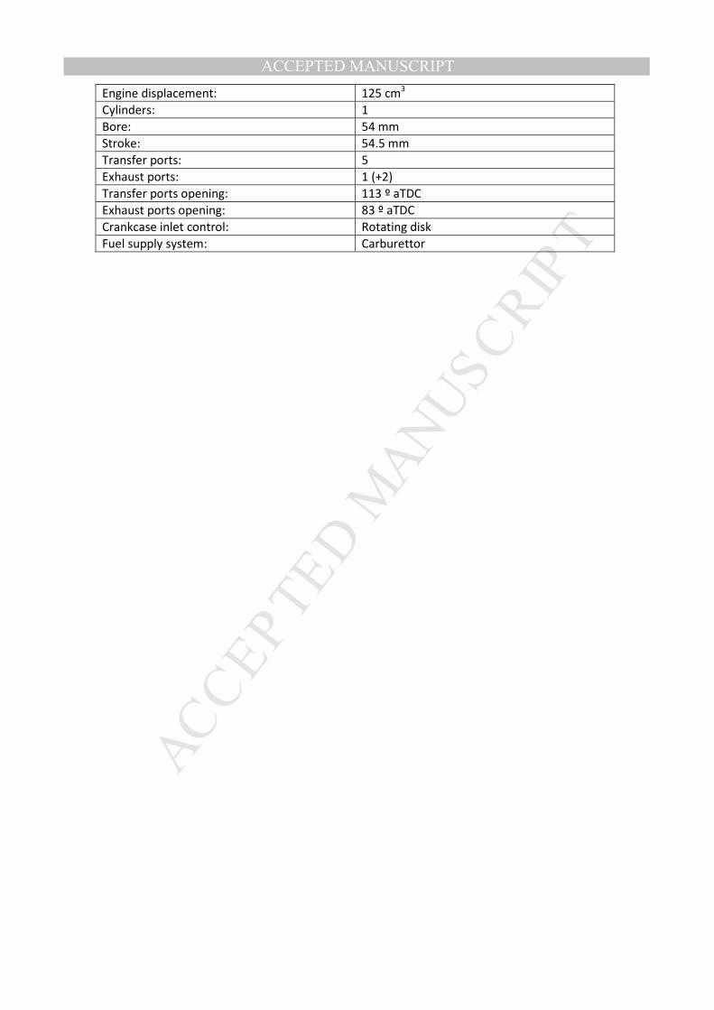
ratio, scavenge efficiency and trapping efficiency. Fig. 3 illustrates the classical representation

for scavenge evaluation. The delivery ratio is the relation between the measured mass through

the intake system, msupplied, and the mass that ideally would enter into the cylinder taking into

account the engine displacement and the density at some reference conditions, mref. The

scavenging efficiency is the ratio between the fresh mixture trapped in the cylinder, mtrapped, and

the total mass in the cylinder for the next engine cycle, mcharge. Therefore, the scavenging

efficiency evaluates the residuals that remain inside the cylinder from the previous cycle. The

MANUSCRIP

T

ACCEPTED

ACCEPTED MANUSCRIPTtrapping efficiency evaluates the short-circuit phenomenon and is calculated with the fresh

mixture trapped in the cylinder, mtrapped, divided by the intake mass, msupplied.

2.2 Heat transfer model

From the different models that account for the turbulence decay found in the literature [9-13], an

example is the one proposed by Farrugia [11], where the Nusselt number is corrected with the

following parameter:

)/(

Re1 1

Dx

C d

+=ψ (3)

where C1 and d are calibration constants, x is the distance from the calculation node to the

exhaust port, D is the exhaust valve diameter and Re the cycle-average Reynolds number

calculated in the exhaust valve. Using empirical data from partial and full load conditions from

1000 to 4000 rpm in a 4-stroke spark-ignited engine, Farrugia proposes 0.075 and 0.25, for C1

and d respectively.

The model developed by Zeng [14] takes into account flow velocity fluctuations in the heat

transfer coefficient determination. The correction to the Nusselt number is given by:

b

t

u

u

DC

+=d

d1

22ψ (4)

where C2 and b are calibration constants, u is the gas particle velocity and D is the valve

diameter.

The proposed model in this paper takes into account the two described phenomena: on one

side, the entrance length and turbulence decay from the exhaust port section, and, on the other

side, the velocity fluctuation of the flow. The former is estimated by using the distance from the

calculation node, x, to the exhaust port cross section. The latter is determined by computing the

variation of the velocity in the calculation node with time, du/dt. A new dimensionless number

derived from the multiplication of both terms, also in non-dimensional approach, is proposed:

=Φt

u

u

D

Dx d

d

/

12

(5)

where x is the distance from the calculation node to the exhaust port, u is the gas particle

velocity and D is the diameter in the considered cross section. As it is observed, the first

MANUSCRIP

T

ACCEPTED

ACCEPTED MANUSCRIPTparenthesis in Eq. (5) is related to the entrance length effects, since calculation nodes close to

the exhaust port provide higher values of Φ. In the same way, a high velocity fluctuation, which

is accounted in absolute value in the second parenthesis, lead to higher values of Φ as well.

The combination of the two effects is important for the model calibration and assessment. The

multiplication of the two parentheses in Eq. (5) means that the model will not capture the

turbulence decay effect in a situation where there is not velocity fluctuation and vice versa.

However, this model description has not limited the results as it will be later demonstrated.

Based on the Reynolds analogy, which relates the friction coefficient with dimensionless

numbers of Stanton, Nusselt, Reynolds and Prandtl, and using the Chilton-Colburn analogy, the

proposed model by Dittus-Boelter can be obtained [2]. If the proposed dimensionless number in

Eq. (5) is included in this expression we get:

2

dd

1PrRe023.0Nu

2

2

133.08.0

V

t

u

ux

DV

+=Φ (6)

where V1 and V2 are two calibration constants obtained experimentally. With the proposed

Nusselt number correction, Eq. (6) can be applied anywhere in the exhaust system, and it is

valid for both steady and pulsating flow.

The parameter q shown in Eq. (2), concerning the energy conservation equation inside the duct,

represents the heat power per unit of mass flow and it is a source term in the partial differential

equations system that is obtained using:

m

Qq

&

&

= (7)

where m& represents the mass flow through the mesh and Q& is obtained using Newton’s law of

cooling, since radiation heat transfer is neglected:

( )wg TTxDhQ −∆= Φ π& (8)

where Φh is the unsteady heat transfer coefficient, x∆ is the spatial mesh length (distance

between calculation nodes), gT the gas temperature and wT the inner wall duct temperature.

The inner wall duct temperature is assumed to be very similar to the outer wall duct temperature

due to two reasons: (i) the reduced thickness of the sheet of exhaust system (2 mm), and (ii) the

high thermal conductivity of the material. The external wall temperature is obtained

MANUSCRIP

T

ACCEPTED

ACCEPTED MANUSCRIPTexperimentally using an infrared thermal camera, which allows estimating the temperature

distribution along the exhaust system. This measured temperature profile is an input to the

engine simulation.

The local convection coefficient is obtained using the corrected Nusselt number defined in Eq.

(6) and the following expression:

D

kh Φ

Φ = Nu (7)

where k is the fluid thermal conductivity, which is assumed to be similar to the air.

3. EXPERIMENTAL SETUP

A two−stroke engine, whose main features are shown in Table 1, was employed in the present

study. The engine is a spark−ignited, crankcase−scavenged type and single−cylinder engine

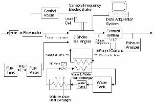
traditionally used in racing applications. A test bench, shown schematically in Fig. 4, was fully

instrumented to carry out performance measurements. Main measurement devices consisted of

an eddy−current electric brake (up to 175 kW), a hot wire anemometer to measure the air mass

flow entering the engine and a gravimetric balance to register the fuel consumption.

Firing tests were carried out at different load and engine speed conditions, since an electronic

module controlled the brake as well as the throttle position. The engine has liquid cooled

cylinder, therefore a second cooling system was designed in order to control the engine coolant

temperature.

Fluid flow properties are also relevant in checking the accuracy of the model. Cycle average

temperature and pressure were measured at the intake and exhaust pipes with thermocouples

and manometers. Also, the external wall temperature was captured with an infrared camera [23]

to aid the 1D engine model. Moreover, pressure transducers were placed in the cylinder,

crankcase, and exhaust port in order to measure its instantaneous evolution (every 0.5 crank

angle degree) following the indications given in [24].

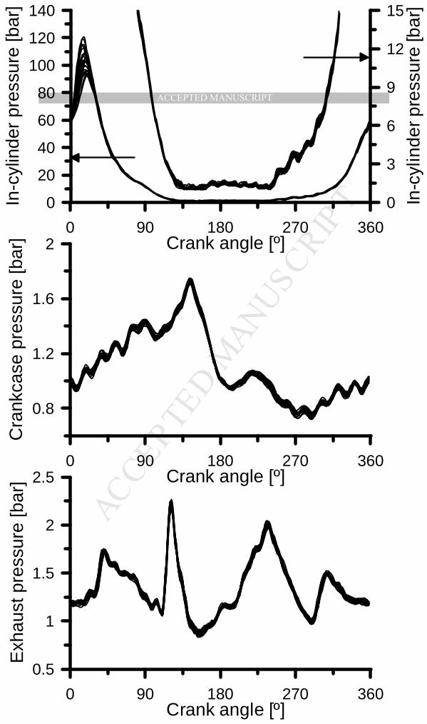
Fig. 5 shows the pressure traces for 25 consecutive engine cycles at a certain engine operating

condition. Measurements are acquired inside the cylinder (top plot), in the crankcase (middle

plot) and in the exhaust system close to the exhaust port (bottom plot), where 0 cad represents

the top dead centre of the piston. For the presented study, it is important to remark that

pressure evolutions in the exhaust system do not show the in-cylinder cycle-to-cycle variation,

MANUSCRIP

T

ACCEPTED

ACCEPTED MANUSCRIPTwhich is typical of spark-ignited engines [25]. This is due to the fact that the in-cylinder pressure

after the combustion process collapses into very similar expansion lines, and in-cylinder

conditions are comparable at the exhaust port opening angle. This behaviour is checked for all

engine running conditions presented in this research.

Concerning the exhaust instantaneous pressure, it is detected a sudden increase after 90 cad,

due to the cylinder blow down when the exhaust port opens. The generated pressure pulse

travels through the exhaust system and reflects as depression waves in a first stage when

evolving inside the divergent pipe, and as overpressure waves when the convergent pipe is

encountered. These depression and overpressure waves travel back to the cylinder and are

clearly detected by the pressure measurement (at 150 and 240 cad respectively, in the plotted

engine running condition). The exhaust pressure evolutions always follow the described pattern

and, if synchronised properly, help to extract the exhaust gases from the cylinder at the

beginning of the scavenge process and retain the fresh mixture before closing the exhaust port.

The instantaneous pressure plotted in the crank-angle domain depends mainly on the engine

speed. Although wave propagation phenomena are modified by the sound speed, exhaust

gases temperature does not change largely within tested engine conditions. Therefore, engine

performance relies very much on the design of the so-called tuned exhaust system geometry

and engine speed.

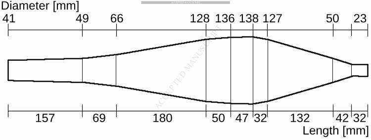
Fig. 6 represents a schematic layout of the exhaust system, where basic geometrical data are

given. Exhaust system pressure evolutions are acquired in three locations along the exhaust

system. The distances from the exhaust port are: 200, 349 and 471 mm. The choice of these

points is not arbitrary: transducer #1 was placed in a point very close to the exhaust port and,

therefore, it is very important from the unsteady flow behaviour point of view. Moreover, this

transducer is placed in the first third of the divergent pipe, where the reflected pulses are

generated. Transducer #2 was positioned in the second third of the divergent duct of the

exhaust system. Finally, transducer #3 was placed in the straight pipe between the divergent

and convergent cones of the exhaust system, where the diameter is the largest. Therefore, the

amplitude of the pressure pulses is low due to the large cross section value.

4. MODELS CALIBRATION

MANUSCRIP

T

ACCEPTED

ACCEPTED MANUSCRIPTDifferent heat transfer models are compared in order to evaluate their behaviour and show their

main advantages and disadvantages. Three models were calibrated in the simplest geometry of

an exhaust system: a constant cross section duct. In this way, modelling uncertainties related to

cross section variations are avoided. Therefore, the experimental setup consists of a straight

duct as exhaust system (39.35 mm in diameter and 458 mm in length) equipped with

piezoelectric and piezoresistive pressure transducers. These are placed on two different

sections, located at 100 and 230 mm from the exhaust port respectively. Besides, average gas

and wall temperatures are measured at the same points by means of K-type thermocouples.

This exhaust system allows engine testing under a wide range of operating conditions between

7000 and 11000 rpm. Engine operation was not steady enough outside these engine speeds

since pressure wave propagation phenomena configure a poor scavenge process with high

concentration of residual gases inside the cylinder, which promoted misfire events.

The straight exhaust system geometry is incorporated in the previously described 1D engine

model, where the following heat transfer models for the exhaust systems are tested: (i) Farrugia

[11], related to the turbulence decay and governed by Eq. (3), (ii) Zeng [14], which accounts for

the flow velocity fluctuations and controlled by Eq. (4), and (iii) the proposed model shown in

Eg. (6).

The calibration of the constants in the models, gathered in Eqs. (3), (4) and (6), is performed by

means of engine simulations. Simulations were run from 7000 to 11000 rpm every 500 rpm.

Each steady state engine running condition was tested with the three heat transfer models.

Each heat transfer model has two calibration constants, which were modified according to the

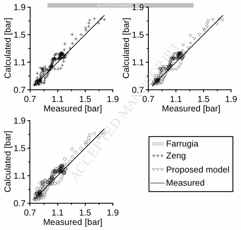
values given in Table 2. A comparison between calculated and measured exhaust

instantaneous pressure is performed for model assessment. Pressure evolutions at transducer

#1 location are analyzed since it is the most critical point for the evaluation of the heat transfer

in the exhaust system. Fig. 7 shows an example of this comparison at 10500 rpm, where the

calculated pressure evolutions in the three models for a given set of calibration constants are

plotted against the measured data. The points in the upper right zone of each plot represent the

cylinder blow down when the exhaust port opens. On the contrary, the points in the lower left

zone of the graph correspond to the cylinder scavenge process or when the exhaust port is

MANUSCRIP

T

ACCEPTED

ACCEPTED MANUSCRIPTclosed. It is observed that a representation of the results as Fig. 7 shows is not useful to provide

a good quality analysis for models comparison.

The coefficient of determination (R2) between measured and calculated data in transducer #1

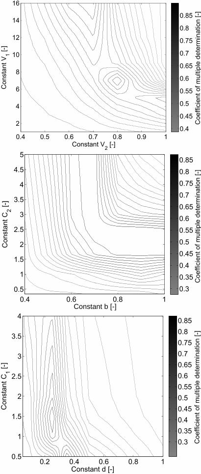
location seems to be an appropriate parameter to quantify the model prediction. Fig. 8 shows

the results in terms of R2 obtained from the simulation matrix given in Table 2, at 10500 rpm,

where the optimum values for the calibration constants are found. Other correlations for the

turbulence decay modelling found in the literature previously referenced were also evaluated

but, after recalibration of their constants values, the results provided similar or less accurate

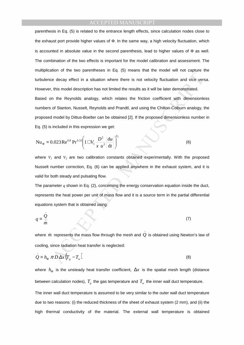
predictions than Farrugia’s correlation.

If Farrugia’s model calibration constants, C1 and d, are set to 1.5 and 0.25, there is an optimum

in the coefficient of determination at 10500 rpm, as depicted in the bottom plot. In the middle

plot, it is observed that Zeng’s model calibration constants, C2 and b, are not easily defined by a

pair of values. The optimum values resemble very much to the shape of an equilateral

hyperbola, which means that high R2 values are obtained with low b and high C2 values or vice

versa. If b value is set to 0.8, as proposed by Zeng, the value for C2 must be 2 in order to

maximize R2. Values for the proposed model are presented in the upper plot, where V1 and V2

should be set to 7 and 0.8 respectively. Overall, by looking at the colour-bar of the three plots, it

is detected that all the models provide good quality values for the coefficient of determination.

For brevity reasons, only the results at 10500 rpm are presented in the paper. However, it

should be mentioned that similar values have been obtained in different engine running

conditions with the straight duct as exhaust system.

5. RESULTS AND DISCUSSION

The predictions of the three heat transfer models using the current exhaust system geometry

are presented in this section. It is important to remark that the same constants values obtained

with the straight-duct exhaust system have been employed. Experimental information from three

sources is used for models’ assessment: the instantaneous pressure measured in locations #1,

#2 and #3 in the exhaust system, the delivery ratio and, finally, the engine BMEP.

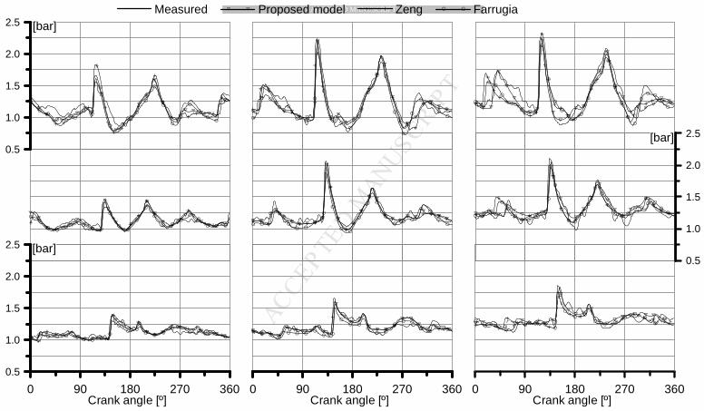
Fig. 9 shows a matrix of plots containing the exhaust pressure traces in three engine speeds:

9500 (left column), 11500 (middle column) and 12500 rpm (right column), and the different

MANUSCRIP

T

ACCEPTED

ACCEPTED MANUSCRIPTtransducers locations: #1 (top row), #2 (middle row) and #3 (bottom row). In each plot there is a

comparison between the heat transfer models together with the measured data. It is important

to remark that the parameters for the Nusselt correlation are the same as the presented before

with the straight duct as exhaust pipe. Main differences appear at 12500 rpm and location #1

(top right plot). In this case the proposed model predicts with better accuracy the measured

exhaust pressure than the other two models. This fact is observed in the prediction of the

depression wave that occurs before BDC (180 cad) and also in the pressure wave that remains

in the exhaust system when the exhaust port is closed, as detected in the overpressure wave at

40 cad.

Although, in general terms, good predictions are observed for all heat transfer models

concerning the instantaneous pressure profile in both amplitude and synchronization of

pressure pulses, it is necessary to check the influence of the slight discrepancies on the engine

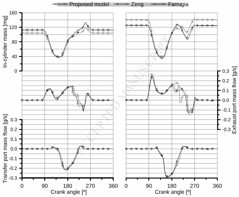
scavenge process. Fig. 10 shows a matrix of plots containing two engine speeds: 9500 (left

column) and 12500 rpm (right column), and the calculated results in terms of: the instantaneous

in-cylinder mass (top row), and the exhaust (middle row) and intake (bottom row) mass flows. A

positive value of the mass flow means that the flow is coming out from the cylinder. Negative

values occur when backflows appear. A typical situation is the exhaust mass flow going into the

cylinder before closing the exhaust port due to the overpressure wave created in convergent

pipe of the exhaust system.

Exhaust mass flows in Fig. 10 present remarkable differences between the different models in

the period from BDC and the exhaust port closing. Slight discrepancies are also found in the

same period for the intake mass flow. Both intake and exhaust mass flows configure the

evolution of the in-cylinder mass, which can lead up to 20% variation in total trapped mass as

observed in the top graphs. The differences in the exhaust mass flow evolutions in the period

from port opening to BDC are not relevant between the three models since the exhaust process

is dominated by the high values of the in-cylinder pressure during the expansion stroke. The

intake mass flow mainly depends on the pressure difference between the crankcase and the

cylinder and irrelevant differences are found until the piston arrives to the BDC. The influence of

the exhaust pressure in the cylinder becomes important once the piston achieves the BDC.

MANUSCRIP

T

ACCEPTED

ACCEPTED MANUSCRIPTFrom this point exhaust heat transfer modelling provides significant differences in the predicted

scavenge process.

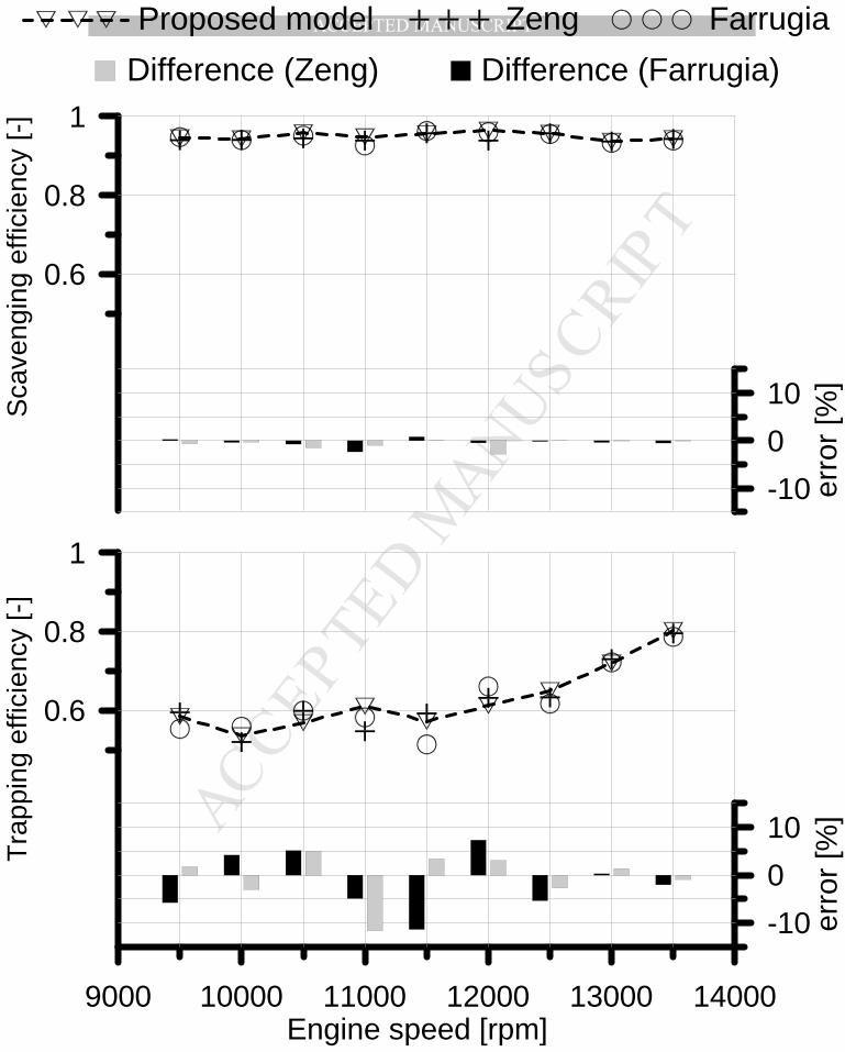
As introduced in Fig. 3, comparisons of the predicted scavenging and trapping efficiencies are

provided in Fig. 11. Each plot presents not only the absolute values but also the difference in

percentage related to the proposed model. Top graph shows the scavenging efficiency. It is

important to remark that the predicted values are between 0.9 and 1, with very reduced

differences among the three models. The design of a high-performance engine leads to

minimize the residual gases from the previous engine cycle and, as other systems, the exhaust

system geometry is conceived to promote an efficient extraction of the exhaust gases from the

cylinder. On the other side, trapping efficiency values are in the range between 0.5 and 0.8,

which means that a large amount of the supplied fresh mixture becomes short-circuit mass,

directly to the exhaust system without being burnt. Trapping efficiency increases with engine

speed as the backflow created by the convergent pipe in the exhaust system and described in

Fig. 10 is better synchronized with exhaust port closing. Besides the engine behaviour and the

absolute values of the trapping efficiency, a relevant issue is the significant differences provided

by the three exhaust heat transfer models. When compared to the proposed model, variations

up to 10% are found in the Farrugia and Zeng models depending on the engine speed. These

differences in the short-circuit prediction influence on the fuel trapped for the next engine cycle

and lead to divergences in the predicted engine performance.

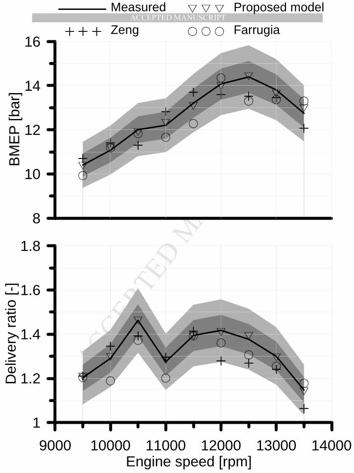
Fig. 12 compares the predicted results with measured data concerning delivery ratio (bottom)

and brake mean effective pressure (top). Measurements are plotted in solid line and two gray

zones are depicted too. Dark gray zone corresponds to points with variations less than ±5%,

while the light gray zone includes errors up to ±10%. All the models predict with great accuracy

the delivery ratio at 9500 and 11500 rpm. The majority of predicted values fall inside the ±5%

error zone. However, the model that accounts for entrance length (circle symbols) provides low

values of supplied mass at lower engines speeds. On the contrary, the model that considers the

velocity fluctuations (cross symbols) underestimate the mass flow at higher engine speeds. The

proposed model provides good predictions for all the range of engine speeds.

The explanation to these cycle-averaged results is found in the instantaneous mass flow

evolutions as shown for two engine speeds in Fig. 10. As an example, the supplied mass at

MANUSCRIP

T

ACCEPTED

ACCEPTED MANUSCRIPT12500 rpm is well captured by the proposed model while higher errors appear with the other two

models. Analyzing in more detail the plots on the right of Fig. 10 (12500 rpm) it is detected that

intake mass flow (bottom plot) is higher in the proposed model in the period after BDC. The

reason to this higher intake mass flow is closely related with the exhaust mass flow (middle plot)

evolution which, finally, is governed by the instantaneous pressure in the exhaust system (as

illustrated in the differences found in the top right corner of Fig. 9).

An interesting result of the presented work is to analyze the influence that the discrepancies in

the scavenging related parameters has in engine performance. Again, most of the predicted

results show errors below ±5% in terms of BMEP. The results from the proposed model

correlate with great accuracy the measured data. The other two models present errors higher

than ±5% at different engine speeds. It should be mentioned that BMEP and delivery ratio

results do not have to correlate since the trapping efficiency also influences on the BMEP.

6. CONCLUSIONS

The heat transfer in the exhaust system of high-performance two-stroke engines was

investigated. Different models from the literature, which take into account the entrance length

and the flow velocity fluctuations, together with a proposed one that combines the two

phenomena, were included in the frame of a 1D engine simulation code.

A 125 cc engine was tested under wide open throttle conditions in a fully instrumented engine

test bench. Three pressure transducers were placed in the exhaust system to capture wave

propagation phenomena. The calibration of the parameters of the three models was performed

with engine tests using a straight pipe with constant transversal section as exhaust system. The

constants values are valid for all the range of tested conditions.

Models assessment was carried out by comparing the predicted results with the measured

exhaust pressure traces in three locations along the exhaust system. The slight differences

found in the pressure signals are better analyzed when observing the predicted mass flows

through the transfer and exhaust ports. Models comparison is finally performed by using

scavenge process related parameters and the influence on BMEP.

Since this type of engines are designed for high performance operation, cylinder ports and

exhaust system geometry are conceived to minimize the residual burnt gases that would remain

MANUSCRIP

T

ACCEPTED

ACCEPTED MANUSCRIPTinside the cylinder for the next engine cycle. Therefore, the scavenging efficiency predicted by

the three models is higher than 0.9 and the differences between the models do not exceed 3%.

However, variations up to 12% are found when comparing the calculated trapping efficiency

among the models.

Finally, the proposed model results in terms of delivery ratio and BMEP provide differences with

measured data lower than 3% for the investigated range of engine speeds. However, the model

that accounts for entrance length and the one that relies on the flow velocity fluctuations predict

differences in the delivery ratio values between 5% and 10% at certain engine speeds. Similar

conclusion is derived for the BMEP results. The combined heat transfer model is able to predict

engine performance for a wide range of engine speeds although the number of calibration

parameters is two for all the models.

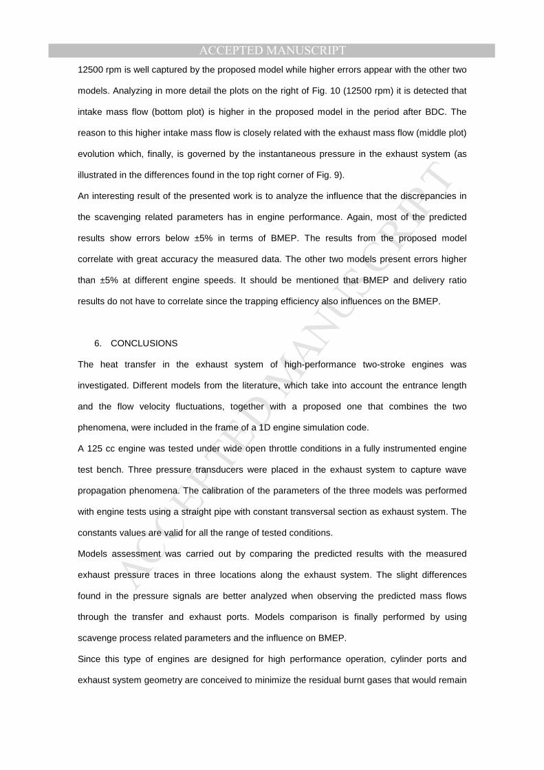
NOMENCLATURE

b constant in Zeng’s correlation

C source term vector

C1 constant in Farrugia’s correlation

C2 constant in Zeng’s correlation

d constant in Farrugia’s correlation

D diameter

F flux vector

g friction

h heat transfer coefficient

k thermal conductivity

Nu Nusselt number

p pressure

Pr Prandtl number

q heat

Re Reynolds number

S cross section

t time

MANUSCRIP

T

ACCEPTED

ACCEPTED MANUSCRIPTT temperature

u gas velocity

V1 constant in proposed correlation

V2 constant in proposed correlation

W state vector

x spatial coordinate

Greek symbols

γ specific heat ratio

ρ density

Subscripts

g gas

w wall

REFERENCES

[1]. J. Galindo, J.R. Serrano, H. Climent, A. Tiseira, Analysis of gas−dynamic effects in

compact exhaust systems of small two−stroke engines, International Journal of

Automotive Technology 8 (N4) (2007) 403−411.

[2]. F.W. Dittus, L.M.K. Boelter, Heat transfer in automobile radiators of the tubular type.

University of California, Berkley Publications on Engineering 2 (13) (1930) 443−461.

[3]. E.N. Sieder, G. E. Tate, Heat transfer and pressure drop of liquids in tubes, Ind. Eng.

Chem. 28 (12) (1936) 1429–1435.

[4]. E.W. Huber, T. Koller, Pipe Friction and Heat Transfer in the Exhaust Pipe of a Firing

Combustion Engine, Proceedings of the CIMAC Convention, Tokio, (1977) 2075−2105.

[5]. D.W. Wendland, Automobile Exhaust−System Steady−State Heat, SAE Paper (1993)

931085.

[6]. P.J.Shayler C.M. Harb, T. Ma, Time−Dependent Behaviour of Heat Transfer Coefficients

for Exhaust Systems, IMechE Paper C496/046/95, VTMS 2 Conf. Proc., 1995.

[7]. C. Depcik D. Assanis, A Universal Heat Transfer Correlation for Intake and Exhaust Flows

in a Spark−Ignition Internal Combustion Engine, SAE Paper (2002) 2002−01−0372.

MANUSCRIP

T

ACCEPTED

ACCEPTED MANUSCRIPT[8]. E.A.M. Elshafei, M. Safwat Mohamed, H. Mansour, M. Sakr, Experimental study of heat

transfer in pulsating turbulent flow in a pipe, International Journal of Heat and Fluid Flow

29 (4) (2008) 1029−1038.

[9]. J. Benajes, A.J., Torregrosa, M. Reyes, Heat Transfer Model for I.C. Engine Exhaust

Manifolds, Proc. Seminair Eurotherm 15 Transferts de Chaleur dans le Moteurs a

Combustion Interne, Tolouse, 1991.

[10]. W.D. Bauer, J. Wenisch, J.B. Heywood, Averaged and time−resolved heat transfer of

steady and pulsating entrance length flow in intake manifolds of a spark−ignition engine,

International Journal of Heat and Fluid Flow 19 (1998) 1−9.

[11]. M. Farrugia, A.C. Alkidas, P. Sangeorzan, Cycle−Average Heat Flux Measurements in

a Straight−Pipe Extension of an Exhaust Port of an SI Engine, SAE Paper (2006)

2006−01−1033.

[12]. A. Sorin, F. Bouloc, B. Bourouga, P. Anthoine, Experimental study of periodic heat

transfer coefficient in the entrance zone of an exhaust pipe, International Journal of

Thermal Sciences 47 (2008), 1665-1675.

[13]. N. Balzan, B.P. Sangeorzan, A.C. Alkidas, Steady−State Local Heat Flux

Measurements in a Straight−Pipe Extension of an Exhaust Port of a Spark Ignition

Engine, SAE Paper (2007) 2007−01−3990.

[14]. P. Zeng, D.N. Assanis, Unsteady convective heat transfer modeling and application to

engine intake manifolds, Proceedings of the ASME International Mechanical Engineering

Congress and R&D Expo (2004) Paper 2004−60068.

[15]. J. Galindo, J.R. Serrano, F.J. Arnau, P. Piqueras, Description of a Semi-Independent

Time Discretization Methodology for a One-Dimensional Gas Dynamics Model, Journal of

Engineering for Gas Turbines and Power 131 (3) (2009).

[16]. J. Galindo, H. Climent, B. Pla, V.D. Jiménez, Correlations for Wiebe Function

Parameters for Combustion Simulation in Two−Stroke Small Engines, Applied Thermal

Engineering, 31 (2011) 1190−1199.

[17]. F. Payri, J.M. Desantes, A.J. Torregrosa, Acoustic boundary conditions for unsteady

one−dimensional flow calculations, Journal of Sound and Vibration, 188 (1) (1995)

85−110.

MANUSCRIP

T

ACCEPTED

ACCEPTED MANUSCRIPT[18]. F. Payri, J.M. Desantes, A. Broatch, Modified impulse method for the measurement of

the frequency response of acoustic filters to weakly nonlinear transient excitations,

Journal of the Acoustic Society of America, 107 (2) (2000) 731−738.

[19]. H. Daneshyar, One−Dimensional Compressible Flow, Oxford, Pergamon Press, Ltd.,

1976.

[20]. D.E. Winterbone, R.J. Pearson, A Solution of the Wave Equations Using Real Gases,

International Journal of Mechanical Sciences 34 (N12) (1992) 917−932.

[21]. A. Harten, High resolution schemes for hyperbolic conservation laws, Journal of

Computational Physics, 49 (3) (1983) 357-393.

[22]. G.P. Blair, Design and simulation of two−stroke engines, R−161 Society of Automotive

Engineers, Inc. Warrendale, PA. 1995.

[23]. V.Macián, B. Tormos, P. Olmeda, R.W. Peralta, Fault detection in diesel engines using

infrared thermography Insight, 44 (2002) 228-232..

[24]. J. Benajes, V. Bermúdez, H. Climent, M.E. Rivas-Perea, Instantaneous pressure

measurement in pulsating high temperature internal flow in ducts, Applied Thermal

Engineering, 61 (2013) 48−54.

[25]. N. Ozdor, M. Dulger, E. Sher, Cyclic Variability in Spark Ingnition Engines A Literature

Survey, SAE Paper (1994) 940987.

MANUSCRIP

T

ACCEPTED

ACCEPTED MANUSCRIPTTABLES CAPTION

Table 1. Engine main characteristics.

Table 2. Simulation matrix for heat transfer models calibration.

MANUSCRIP

T

ACCEPTED

ACCEPTED MANUSCRIPTFIGURES CAPTION

Fig 1. Exhaust port instantaneous pressure at 12500 rpm and full load: measured (solid line)

and calculated (dashed line) with Dittus-Boelter correlation.

Fig 2. Schematic layout of the 1D engine model.

Fig 3. Masses definition for scavenge process evaluation.

Fig 4. Schematic layout of the engine test bench.

Fig 5. Cycle-to-cycle pressure variations in the cylinder (top), crankcase (middle) and exhaust

system (bottom) at 12500 rpm.

Fig 6. Schematic layout of the 125 cc engine exhaust system.

Fig 7. Comparison between measured and calculated exhaust pressure with the straight duct as

exhaust system at 10500 rpm.

Fig 8. Coefficient of determination in the parameters calibration process at 10500 rpm for the

heat transfer models: proposed (top), Zeng (middle) and Farrugia (bottom).

Fig 9. Measured and calculated instantaneous exhaust pressure in transducers #1 (top), #2

(middle) and #3 (bottom) at 9500 (left), 11500 (middle) and 12500 rpm (right).

Fig 10. Calculated instantaneous in-cylinder mass (top) and, exhaust (middle) and intake

(bottom) mass flows at 9500 (left) and 12500 rpm (right).

Fig 11. Calculated scavenging efficiency (top) and trapping efficiency (bottom).

Fig 12. Measured and calculated BMEP (top) and delivery ratio (bottom).

MANUSCRIP

T

ACCEPTED

ACCEPTED MANUSCRIPTEngine displacement: 125 cm

3

Cylinders: 1

Bore: 54 mm

Stroke: 54.5 mm

Transfer ports: 5

Exhaust ports: 1 (+2)

Transfer ports opening: 113 º aTDC

Exhaust ports opening: 83 º aTDC

Crankcase inlet control: Rotating disk

Fuel supply system: Carburettor

MANUSCRIP

T

ACCEPTED

ACCEPTED MANUSCRIPTModel Parameter Range

Farrugia C1 0.5-4

d 0.1-1

Zeng C2 0.4-5

b 0.4-1

Proposed V1 1-16

V2 0.4-1

MANUSCRIP

T

ACCEPTED

ACCEPTED MANUSCRIPT

0 90 180 270 360Crank angle [º]

0.5

1.0

1.5

2.0E

xha

ust

pre

ssu

re [

bar]

Measured Dittus-Boelter

MANUSCRIP

T

ACCEPTED

ACCEPTED MANUSCRIPT

MANUSCRIP

T

ACCEPTED

ACCEPTED MANUSCRIPT

mtrapped

mcharge

mresiduals

mshort-circuit

msupplied

mref

MANUSCRIP

T

ACCEPTED

ACCEPTED MANUSCRIPT

MANUSCRIP

T

ACCEPTED

ACCEPTED MANUSCRIPT

0 90 180 270 360Crank angle [º]

0

20

40

60

80

100

120

140In

-cyl

inde

r pr

essu

re [b

ar]

0.5

1

1.5

2

2.5

Exh

aust

pre

ssur

e [b

ar]

0 90 180 270 360Crank angle [º]

0.8

1.2

1.6

2

Cra

nkca

se p

ress

ure

[bar

]

0 90 180 270 360Crank angle [º]

0

3

6

9

12

15

In-c

ylin

de

r p

ress

ure

[ba

r]

MANUSCRIP

T

ACCEPTED

ACCEPTED MANUSCRIPTDiameter [mm]41 49 66 128 136 138 127 50 23

Length [mm]157 69 180 50 47 13232 42 32

MANUSCRIP

T

ACCEPTED

ACCEPTED MANUSCRIPT

0.7 1.1 1.5 1.9Measured [bar]

0.7

1.1

1.5

1.9

Ca

lcu

late

d [

ba

r]

0.7 1.1 1.5 1.9Measured [bar]

0.7

1.1

1.5

1.9C

alcu

late

d [b

ar]

0.7

1.1

1.5

1.9

Cal

cula

ted

[bar

]

0.7 1.1 1.5 1.9Measured [bar]

Measured

Zeng

Proposed model

Farrugia

MANUSCRIP

T

ACCEPTED

ACCEPTED MANUSCRIPT

Con

stan

t V1 [-

]

0.4 0.5 0.6 0.7 0.8 0.9 1

2

4

6

8

10

12

14

16

0.4

0.45

0.5

0.55

0.6

0.65

0.7

0.75

0.8

0.85C

onst

ant C

2 [-]

0.4 0.6 0.8 10.5

1

1.5

2

2.5

3

3.5

4

4.5

5

0.30.350.40.450.50.550.60.650.70.750.80.85

Constant d [-]

Con

stan

t C1 [-

]

0.2 0.4 0.6 0.8 10.5

1

1.5

2

2.5

3

3.5

4

0.30.350.40.450.50.550.60.650.70.750.80.85

Coe

ffici

ent o

f mul

tiple

det

erm

inat

ion

[-]C

oeffi

cien

t of m

ultip

le d

eter

min

atio

n [-]

Coe

ffici

ent o

f mul

tiple

det

erm

inat

ion

[-]

Constant V2 [-]

Constant b [-]

MANUSCRIP

T

ACCEPTED

ACCEPTED MANUSCRIPT

0 90 180 270 360Crank angle [º]

0.5

1.0

1.5

2.0

2.5

0 90 180 270 360Crank angle [º]

[bar]0.5

1.0

1.5

2.0

2.5 [bar]

0.5

1.0

1.5

2.0

2.5 [bar]

0 90 180 270 360Crank angle [º]

[bar]

[bar]

[bar]

Measured ZengProposed model Farrugia

MANUSCRIP

T

ACCEPTED

ACCEPTED MANUSCRIPT

0 90 180 270 360Crank angle [º]

0 90 180 270 360Crank angle [º]

0

40

80

120

160

In-c

ylin

der

mas

s [m

g]

-0.3

-0.2

-0.1

0.0

0.1

0.2

0.3

Exh

au

st p

ort

ma

ss fl

ow

[g/s

]

-0.3

-0.2

-0.1

0.0

0.1

0.2

0.3

Tra

nsfe

r po

rt m

ass

flow

[g/s

]ZengProposed model Farrugia

MANUSCRIP

T

ACCEPTED

ACCEPTED MANUSCRIPT

9000 10000 11000 12000 13000 14000Engine speed [rpm]

0.6

0.8

1

Tra

ppi

ng

eff

icie

ncy

[-]

0.6

0.8

1

Sca

ven

gin

g ef

ficie

ncy

[-]

-10

0

10

err

or [%

]

-10

0

10e

rror

[%]

ZengProposed model Farrugia

Difference (Zeng) Difference (Farrugia)

MANUSCRIP

T

ACCEPTED

ACCEPTED MANUSCRIPT

1

1.2

1.4

1.6

1.8

Deliv

ery

ratio

[-]

9000 10000 11000 12000 13000 14000Engine speed [rpm]

8

10

12

14

16

BM

EP

[ba

r]Measured

Zeng

Proposed model

Farrugia