364
1 LECTURE NOTES ON HEAT & MASS TRANSFER BY DR. T.R.SEETHARAM (NIE, Mysore, India)
| Date post: | 31-Mar-2015 |
| Category: |
Documents |
| Upload: | gary-s-goddard |
| View: | 3,785 times |
| Download: | 21 times |

1
LECTURE NOTES
ON
HEAT & MASS TRANSFER
BY
DR. T.R.SEETHARAM (NIE, Mysore, India)
2
CHAPTER 1
INTRODUCTORY CONCEPTS AND BASIC LAWS
OF HEAT TRANSFER
1.1. Introduction:- We recall from our knowledge of thermodynamics that heat is a form of energy transfer that takes place from a region of higher temperature to a region of lower temperature solely due to the temperature difference between the two regions. With the knowledge of thermodynamics we can determine the amount of heat transfer for any system undergoing any process from one equilibrium state to another. Thus the thermodynamics knowledge will tell us only how much heat must be transferred to achieve a specified change of state of the system. But in practice we are more interested in knowing the rate of heat transfer (i.e. heat transfer per unit time) rather than the amount. This knowledge of rate of heat transfer is necessary for a design engineer to design all types of heat transfer equipments like boilers, condensers, furnaces, cooling towers, dryers etc.The subject of heat transfer deals with the determination of the rate of heat transfer to or from a heat exchange equipment and also the temperature at any location in the device at any instant of time. The basic requirement for heat transfer is the presence of a “temperature difference”. The temperature difference is the driving force for heat transfer, just as the voltage difference for electric current flow and pressure difference for fluid flow. One of the parameters ,on which the rate of heat transfer in a certain direction depends, is the magnitude of the temperature gradient in that direction. The larger the gradient higher will be the rate of heat transfer. 1.2. Heat Transfer Mechanisms:- There are three mechanisms by which heat transfer can take place. All the three modes require the existence of temperature difference. The three mechanisms are: (i) conduction, (ii) convection and (iii) radiation 1.2.1Conduction:- It is the energy transfer that takes place at molecular levels. Conduction is the transfer of energy from the more energetic molecules of a substance to the adjacent less energetic molecules as a result of interaction between the molecules. In the case of liquids and gases conduction is due to collisions and diffusion of the molecules during their random motion. In solids, it is due to the vibrations of the molecules in a lattice and motion of free electrons. Fourier’s Law of Heat Conduction:- The empirical law of conduction based on experimental results is named after the French Physicist Joseph Fourier. The law states that the rate of heat flow by conduction in any medium in any direction is proportional to the area normal to the direction of heat flow and also proportional to the temperature gradient in that direction. For example the rate of heat transfer in x-direction can be written according to Fourier’s law as

3
1.2
Qx α − A (dT / dx) …………………….(1.1) Or Qx = − k A (dT / dx) W………………….. ..(1.2) In equation (1.2), Qx is the rate of heat transfer in positive x-direction through area A of the medium normal to x-direction, (dT/dx) is the temperature gradient and k is the constant of proportionality and is a material property called “thermal conductivity”. Since heat transfer has to take place in the direction of decreasing temperature, (dT/dx) has to be negative in the direction of heat transfer. Therefore negative sign has to be introduced in equation (1.2) to make Qx positive in the direction of decreasing temperature, thereby satisfying the second law of thermodynamics. If equation (1.2) is divided throughout by A we have qx = (Qx / A) = − k (dT / dx) W/m2………..(1.3) qx is called the heat flux. Thermal Conductivity:- The constant of proportionality in the equation of Fourier’s law of conduction is a material property called the thermal conductivity.The units of thermal conductivity can be obtained from equation (1.2) as follows: Solving for k from Eq. (1.2) we have k = − qx / (dT/dx) Therefore units of k = (W/m2 ) (m/ K) = W / (m – K) or W / (m – 0 C). Thermal conductivity is a measure of a material’s ability to conduct heat. The thermal conductivities of materials vary over a wide range as shown in Fig. 1.1. It can be seen from this figure that the thermal conductivities of gases such as air vary by a factor of 10 4 from those of pure metals such as copper. The kinetic theory of gases predicts and experiments confirm that the thermal conductivity of gases is proportional to the square root of the absolute temperature, and inversely proportional to the square root of the molar mass M. Hence, the thermal conductivity of gases increases with increase in temperature and decrease with increase in molar mass. It is for these reasons that the thermal conductivity of helium (M=4) is much higher than those of air (M=29) and argon (M=40).For wide range of pressures encountered in practice the thermal conductivity of gases is independent of pressure. The mechanism of heat conduction in liquids is more complicated due to the fact that the molecules are more closely spaced, and they exert a stronger inter-molecular force field. The values of k for liquids usually lie between those for solids and gases. Unlike gases, the thermal conductivity for most liquids decreases with increase in temperature except for water. Like gases the thermal conductivity of liquids decreases with increase in molar mass.

4
1.3
Fig. 1.1: Typical range of thermal conductivities of various materials
In the case of solids heat conduction is due to two effects: the vibration of lattice induced by the vibration of molecules positioned at relatively fixed positions , and energy transported due to the motion of free electrons. The relatively high thermal conductivities of pure metals are primarily due to the electronic component. The lattice component of thermal conductivity strongly depends on the way the molecules are arranged. For example, diamond, which is highly ordered crystalline solid, has the highest thermal conductivity at room temperature. Unlike metals, which are good electrical and heat conductors, crystalline solids such as diamond and semiconductors such as silicon are good heat conductors but poor electrical conductors. Hence such materials find widespread use in electronic industry. Despite their high price, diamond heat sinks are used in the cooling of sensitive electronic components because of their excellent thermal conductivity. Silicon oils and gaskets are commonly used in the packaging of electronic components because they provide both good thermal contact and good electrical insulation.
1000 100 10 1.0 0.1 0.01
k (W/m-K)
Solid metals
Liquid metals
Non- Metallic solids
Non- Metallic liquids
Insulating Materials
Non- Metallic gases
Evacuated Insulating materials
Silver
Copper
Sodium
Steel
Mercury
Oxides
Plastics
Wood
Water
Oils
Fibres
Foams
He, H2
CO2

5
1.4
One would expect that metal alloys will have high thermal conductivities, because pure metals have high thermal conductivities. For example one would expect that the value of the thermal conductivity k of a metal alloy made of two metals with thermal conductivities k1 and k2 would lie between k1 and k2.But this is not the case. In fact k of a metal alloy will be less than that of either metal. The thermal conductivities of materials vary with temperature. But for some materials the variation is insignificant even for wide temperature range.At temperatures near absolute zero, the thermal conductivities of certain solids are extremely large. For example copper at 20 K will have a thermal conductivity of 20,000 W / (m-K), which is about 50 times the conductivity at room temperature. The temperature dependence of thermal conductivity makes the conduction heat transfer analysis more complex and involved. As a first approximation analysis for solids with variable conductivity is carried out assuming constant thermal conductivity which is an average value of the conductivity for the temperature range of interest. Thermal Diffusivity:- This is a property which is very helpful in analyzing transient heat conduction problem and is normally denoted by the symbol α . It is defined as follows. Heat conducted k α = -------------------------------------- = -------- (m2/s) ……(1.4) Heat Stored per unit volume ρCp It can be seen from the definition of thermal diffusivity that the numerator represents the ability of the material to conduct heat across its layers and the denominator represents the ability of the material to store heat per unit volume. Hence we can conclude that larger the value of the thermal diffusivity, faster will be the propagation of heat into the medium. A small value of thermal diffusivity indicates that heat is mostly absorbed by the material and only a small quantity of heat will be conducted across the material. 1.2.2. Convection :- Convection heat transfer is composed of two mechanisms. Apart from energy transfer due to random molecular motion, energy is also transferred due to macroscopic motion of the fluid. Such motion in presence of the temperature gradient contributes to heat transfer. Thus in convection the total heat transfer is due to random motion of the fluid molecules together with the bulk motion of the fluid, the major contribution coming from the latter mechanism. Therefore bulk motion of the fluid is a necessary condition for convection heat transfer to take place in addition to the temperature gradient in the fluid. Depending on the force responsible for the bulk motion of the fluid, convective heat transfer is classified into “forced convection” and “natural or free convection”. In the case of forced convection, the fluid flow is caused by an external agency like a pump or a blower where as in the case of natural or free convection the force responsible for the fluid flow (normally referred to as the buoyancy force) is generated within the fluid itself due to density differences which are caused due to temperature gradient within the flow field. Regardless of the particular nature of convection, the rate equation for convective heat transfer is given by
6
1.5
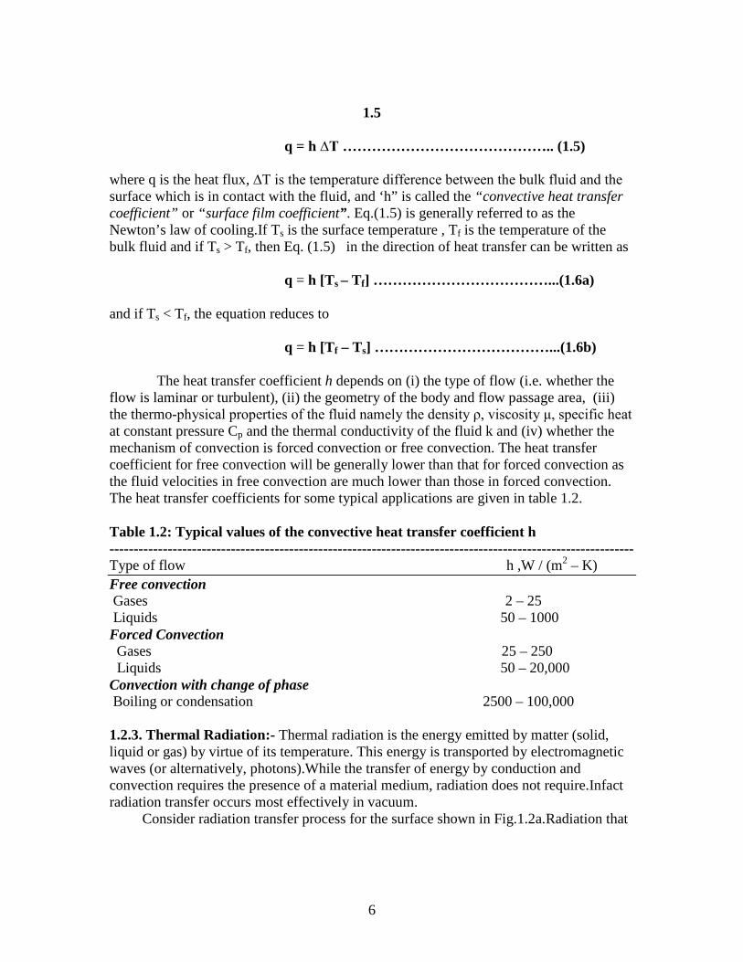
q = h ∆T …………………………………….. (1.5) where q is the heat flux, ∆T is the temperature difference between the bulk fluid and the surface which is in contact with the fluid, and ‘h” is called the “convective heat transfer coefficient” or “surface film coefficient”. Eq.(1.5) is generally referred to as the Newton’s law of cooling.If Ts is the surface temperature , Tf is the temperature of the bulk fluid and if Ts > Tf, then Eq. (1.5) in the direction of heat transfer can be written as q = h [Ts – Tf] ………………………………...(1.6a) and if Ts < Tf, the equation reduces to q = h [Tf – Ts] ………………………………...(1.6b) The heat transfer coefficient h depends on (i) the type of flow (i.e. whether the flow is laminar or turbulent), (ii) the geometry of the body and flow passage area, (iii) the thermo-physical properties of the fluid namely the density ρ, viscosity μ, specific heat at constant pressure Cp and the thermal conductivity of the fluid k and (iv) whether the mechanism of convection is forced convection or free convection. The heat transfer coefficient for free convection will be generally lower than that for forced convection as the fluid velocities in free convection are much lower than those in forced convection. The heat transfer coefficients for some typical applications are given in table 1.2. Table 1.2: Typical values of the convective heat transfer coefficient h ------------------------------------------------------------------------------------------------------------ Type of flow h ,W / (m2 – K) Free convection Gases 2 – 25 Liquids 50 – 1000 Forced Convection Gases 25 – 250 Liquids 50 – 20,000 Convection with change of phase Boiling or condensation 2500 – 100,000
1.2.3. Thermal Radiation:- Thermal radiation is the energy emitted by matter (solid, liquid or gas) by virtue of its temperature. This energy is transported by electromagnetic waves (or alternatively, photons).While the transfer of energy by conduction and convection requires the presence of a material medium, radiation does not require.Infact radiation transfer occurs most effectively in vacuum. Consider radiation transfer process for the surface shown in Fig.1.2a.Radiation that

7
1.6
is emitted by the surface originates from the thermal energy of matter bounded by the surface, and the rate at which this energy is released per unit area is called as the surface emissive power E.An ideal surface is one which emits maximum emissive power and is called an ideal radiator or a black body.Stefan-Boltzman’s law of radiation states that the emissive power of a black body is proportional to the fourth power of the absolute temperature of the body. Therefore if Eb is the emissive power of a black body at temperature T 0K, then
Eb α T 4 Or Eb = σ T 4 ………………………………….(1.7) σ is the Stefan-Boltzman constant (σ = 5.67 x 10 − 8 W / (m2 – K4) ). For a non black surface the emissive power is given by E = ε σ T 4…………………………………(1.8) where ε is called the emissivity of the surface (0 ≤ ε ≤ 1).The emissivity provides a measure of how efficiently a surface emits radiation relative to a black body. The emissivity strongly depends on the surface material and finish. Radiation may also incident on a surface from its surroundings. The rate at which the radiation is incident on a surface per unit area of the surface is calle the “irradiation” of the surface and is denoted by G. The fraction of this energy absorbed by the surface is called “absorptivity” of the surface and is denoted by the symbol α. The fraction of the
G E
Surface of emissivity ε, absorptivity α, and
temperature Ts
Surface of emissivity ε, area
A, and temperature Ts
Surroundings (black) at Tsurr (a) (b)
Fig.1.2: Radiation exchange: (a) at a surface and (b) between a surface and large surroundings
qsurr
q s
ρG

8
1.7 incident energy is reflected and is called the “reflectivity” of the surface denoted by ρ and the remaining fraction of the incident energy is transmitted through the surface and is called the “transmissivity” of the surface denoted by τ. It follows from the definitions of α, ρ, and τ that α+ ρ + τ = 1 …………………………………….(1.9) Therefore the energy absorbed by a surface due to any radiation falling on it is given by Gabs = αG …………………………………(1.10) The absorptivity α of a body is generally different from its emissivity. However in many practical applications, to simplify the analysis α is assumed to be equal to its emissivity ε. Radiation Exchange:- When two bodies at different temperatures “see” each other, heat is exchanged between them by radiation. If the intervening medium is filled with a substance like air which is transparent to radiation, the radiation emitted from one body travels through the intervening medium without any attenuation and reaches the other body, and vice versa. Then the hot body experiences a net heat loss, and the cold body a net heat gain due to radiation heat exchange between the two. The analysis of radiation heat exchange among surfaces is quite complex which will be discussed in chapter 10. Here we shall consider two simple examples to illustrate the method of calculating the radiation heat exchange between surfaces. As the first example’ let us consider a small opaque plate (for an opaque surface τ = 0) of area A, emissivity ε and maintained at a uniform temperature Ts. Let this plate is exposed to a large surroundings of area Asu (Asu >> A) whish is at a uniform temperature Tsur as shown in Fig. 1.2b.The space between them contains air which is transparent to thermal radiation. The radiation energy emitted by the plate is given by Qem = A ε σ Ts
4 The large surroundings can be approximated as a black body in relation to the small plate. Then the radiation flux emitted by the surroundings is σ Tsur
4 which is also the radiaton flux incident on the plate. Therefore the radiation energy absorbed by the plate due to emission from the surroundings is given by Qab = A α σ Tsur
4. The net radiation loss from the plate to the surroundings is therefore given by Qrad = A ε σ Ts
4 − A α σ Tsur4.

9
1.8 Assuming α = ε for the plate the above expression for Qnet reduces to Qrad = A ε σ [Ts
4 – Tsur4 ] ……………….(1.11)
The above expression can be used to calculate the net radiation heat exchange between a small area and a large surroundings. As the second example, consider two finite surfaces A1 and A2 as shown in Fig. 1.3.
The surfaces are maintained at absolute temperatures T1 and T2 respectively, and have emissivities ε1 and ε2. Part of the radiation leaving A1 reaches A2, while the remaining energy is lost to the surroundings. Similar considerations apply for the radiation leaving A2.If it is assumed that the radiation from the surroundings is negligible when compared to the radiation from the surfaces A1 and A2 then we can write the expression for the radiation emitted by A1 and reaching A2 as Q1→2 = F1− 2 A1ε1σ T1
4……………………………(1.12) where F1 – 2 is defined as the fraction of radiation energy emitted by A1 and reaching A2. Similarly the radiation energy emitted by A2 and reaching A1 is given by Q2→1 = F2− 1 A2 ε2 σ T2
4 …………………………..(1.13) where F2 – 1 is the fraction of radiation energy leaving A2 and reaching A1. Hence the net radiation energy transfer from A1 to A2 is given by Q1 – 2 = Q1→2 − Q2→1
Surroundings
A1, ε1, T1
A2, ε2, T2
Fig.1.3: Radiation exchange between surfaces A1 and A2

10
1.9 = [F1− 2 A1ε1σ T1
4] − [F2− 1 A2 ε2 σ T24]
F1-2 is called the view factor (or geometric shape factor or configuration factor) of A2 with respect to A1 and F2 - 1 is the view factor of A1 with respect to A2.It will be shown in chapter 10 that the view factor is purely a geometric property which depends on the relative orientations of A1 and A2 satisfying the reciprocity relation, A1 F1 – 2 = A2 F2 – 1.
Therefore Q1 – 2 = A1F1 – 2 σ [ε1 T1
4 − ε2 T24]………………….(1.13)
Radiation Heat Transfer Coefficient:- Under certain restrictive conditions it is possible to simplify the radiation heat transfer calculations by defining a radiation heat transfer coefficient hr analogous to convective heat transfer coefficient as Qr = hrA ΔT For the example of radiation exchange between a surface and the surroundings [Eq. (1. 11)] using the concept of radiation heat transfer coefficient we can write Qr = hrA[Ts – Tsur] = A ε σ [Ts
4 – Tsur4 ]
ε σ [Ts
4 – Tsur4 ] ε σ [Ts
2 + Tsur2 ][Ts + Tsur][Ts – Tsur]
Or hr = --------------------- = ----------------------------------------------- [Ts – Tsur] [Ts – Tsur] Or hr = ε σ [Ts
2 + Tsur2 ][Ts + Tsur] ………………………(1.14)
1.3.First Law of Thermodynamics (Law of conservation of energy) as applied to Heat Transfer Problems :- The first law of thermodynamics is an essential tool for solving many heat transfer problems. Hence it is necessary to know the general formulation of the first law of thermodynamics. First law equation for a control volume:- A control volume is a region in space bounded by a control surface through which energy and matter may pass.There are two options of formulating the first law for a control volume. One option is formulating the law on a rate basis. That is, at any instant, there must be a balance between all energy rates. Alternatively, the first law must also be satisfied over any time interval Δt. For such an interval, there must be a balance between the amounts of all energy changes. First Law on rate basis :- The rate at which thermal and mechanical energy enters a control volume, plus the rate at which thermal energy is generated within the control volume, minus the rate at which thermal and mechanical energy leaves the control volume must be equal to the rate of increase of stored energy within the control volume. Consider a control volume shown in Fig. 1.4 which shows that thermal and

11
1.10
. mechanical energy are entering the control volume at a rate denoted by Ein, thermal and
. mechanical energy are leaving the control volume at a rate denoted by Eout. The rate at . which energy is generated within the control volume is denoted by Eg and the rate at . which energy is stored within the control volume is denoted by Est. The general form of the energy balance equation for the control volume can be written as follows: . . . . Ein + Eg − Eout = Est ……………………………(1.15) . Est is nothing but the rate of increase of energy within the control volume and hence can be written as equal to dEst / dt. First Law over a Time Interval Δt :- Over a time interval Δt, the amount of thermal and mechanical energy that enters a control volume, plus the amount of thermal energy generated within the control volume minus the amount of thermal energy that leaves the control volume is equal to the increase in the amount of energy stored within the control volume. The above statement can be written symbolically as Ein + Eg – Eout = ΔEst …………………………..(1.16)
. Ein
. Eout
. Eg .
Est
Fig. 1.4: Conservation of energy for a control volume on rate basis

12
1.11 The inflow and outflow energy terms are surface phenomena. That is they are associated exclusively with the processes occurring at the boundary surface and are proportional to the surface area. The energy generation term is associated with conversion from some other form (chemical, electrical, electromagnetic, or nuclear) to thermal energy. It is a volumetric phenomenon.That is, it occurs within the control volume and is proportional to the magnitude of this volume. For example, exothermic chemical reaction may be taking place within the control volume. This reaction converts chemical energy to thermal energy and we say that energy is generated within the control volume. Conversion of electrical energy to thermal energy due to resistance heating when electric current is passed through an electrical conductor is another example of thermal energy generation Energy storage is also a volumetric phenomenon and energy change within the control volume is due to the changes in kinetic, potential and internal energy of matter within the control volume. 1.4. Illustrative Examples: A. Conduction
Example 1.1:- Heat flux through a wood slab 50 mm thick, whose inner and outer
surface temperatures are 40 0 C and 20 0 C respectively, has been determined to be 40 W/m2. What is the thermal conductivity of the wood slab?
Solution:
Assuming steady state conduction across the thickness of the slab and noting that the slab is not generating any thermal energy, the first law equation for the slab can be written as Rate at which thermal energy (conduction) is entering the slab at the surface x = 0
L
x
T1
T2
Given:- T1 = 40 0 C; T2 = 20 0 C; L = 0.05 m q = Q/A = 40 W / m2. To find: k .

13
1.12 is equal to the rate at which thermal energy is leaving the slab at the surface x = L That is Qx|x = 0 = Qx|x = L = Qx = constant By Fourier’s law we have Qx = − kA (dT / dx). Separating the variables and integrating both sides w.r.t. ‘x’ we have L T2 Qx ∫dx = − kA ∫dT . Or Qx = kA (T1 – T2) / L
0 T1
Heat flux = q = Qx / A = k(T1 – T2) / L Hence k = q L / (T1 – T2) = 40 x 0.05 / (40 – 20) = 0.1 W / (m – K) Example 1.2:- A concrete wall, which has a surface area of 20 m2 and thickness 30 cm, separates conditioned room air from ambient air.The temperature of the inner surface of the wall is 25 0 C and the thermal conductivity of the wall is 1.5 W / (m-K).Determine the heat loss through the wall for ambient temperature varying from ─ 15 0 C to 38 0 C which correspond to winter and summer conditions and display your results graphically. Solution:
Q
T1
T2
L
Data:- T1 = 25 0 C ; A = 20 m2; L = 0.3 m K = 1.5 W /(m-K) ; By Fourier’s law, Q = kA(T1 – T2) / L 1.5 x 20 x (25 – T2) = ------------------------- 0.30 Or Q = 2500 – 100 T2 ………..(1)
Heat loss Q for different values of T2 ranging from – 15 0 C to + 38 0 C are obtained from Eq. (1) and the results are plotted as shown Scale x-axis : 1cm= 5 C y-axis : 1cm =1000 W

14
1.13
Q 1.2 equation: Q= 2500-100T(2)
-2000
-1000
0
1000
2000
3000
4000
5000
1 2 3 4 5 6 7 8 9 10 11 12
T(2) , celsius
Q ,w
atts
Series2
Example 1.3:-What is the thickness required of a masonry wall having a thermal conductivity of 0.75 W/(m-K), if the heat transfer rate is to be 80 % of the rate through another wall having thermal conductivity of 0.25 W/(m-K) and a thickness of 100 mm? Both walls are subjected to the same temperature difference. Solution:- Let subscript 1 refers to masonry wall and subscript 2 refers to the other wall. By Fourier’s law, Q1 = k1A(T1 – T2) / L1 And Q2 = k2A(T1 – T2) / L2
Therefore Q1 k1 L2 ---- = ---------- Q2 k2 L1 Q2 k1 L1 = ----------- L2 Q1 k2 = (1 / 0.80) x (0.75/0.25) x 100 = 375 mm B. Convection:
Example 1.4:- Air at 40 0 C flows over a long circular cylinder of 25 mm diameter with an embedded electrical heater. In a series of tests, measurements were made of power

15
1.14 per unit length, P required to maintain the surface temperature of the cylinder at 300 0 C for different stream velocities V of the air. The results are as follows:
Air velocity, V (m/s) : 1 2 4 8 12
Power, P (W/m) : 450 658 983 1507 1963
(a) Determine the convective heat transfer coefficient for each velocity and display
your results graphically. (h = P / 20.43) (b)Assuming the dependence of the heat transfer coefficient on velocity to be of the form h = CV n , determine the parameters C and n from the results of part (a). Solution:-
If h is the surface heat transfer coefficient then the power dissipated by the cylinder by convection is given by P = hAs (Ts - T∞) Where As is the area of contact between the fluid and the surface of the cylinder. Therefore P = h πDL (Ts - T∞)
Or h = P / [πDL(Ts - T∞)] = P / [π x 0.025 x 1 x(300 – 40)] Or h = P / 20.42 W/m2-k ………………………………..(1) Values of h for different flow velocities are obtained and tabulated as follows:
V,T∞
Ts
D
Data:- D = 0.025 m : Ts = 300 0 C ; T∞ = 40 0 C;
16
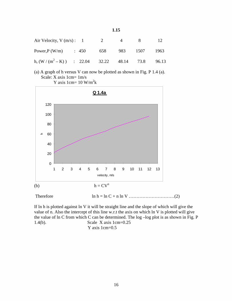
1.15 Air Velocity, V (m/s) : 1 2 4 8 12 Power,P (W/m) : 450 658 983 1507 1963 h, (W / (m2 – K) ) : 22.04 32.22 48.14 73.8 96.13 (a) A graph of h versus V can now be plotted as shown in Fig. P 1.4 (a). Scale: X axis 1cm= 1m/s Y axis 1cm= 10 W/m2k
Q 1.4a
0
20
40
60
80
100
120
1 2 3 4 5 6 7 8 9 10 11 12 13velocity, m/s
h
(b) h = CVn Therefore ln h = ln C + n ln V …………………………(2) If ln h is plotted against ln V it will be straight line and the slope of which will give the value of n. Also the intercept of this line w.r.t the axis on which ln V is plotted will give the value of ln C from which C can be determined. The log –log plot is as shown in Fig. P 1.4(b). Scale X axis 1cm=0.25 Y axis 1cm=0.5

17
1.16
1.4b Slope: 0.571
0
1
2
3
4
5
1 2 3 4 5 6 7 8 9 10 11 12
ln v
ln h
ln C = 3.1 or C = 22 (ln h – ln C) (4.55 – 3.10) and n = ----------------------- = ------------------- ln V 2.5 = 0.571 Therefore h = 22.2 V0.571 is the empirical relation between h and V. Example 1.5:- A large surface at 50 0 C is exposed to air at 20 0 C. If the heat transfer coefficient between the surface and the air is 15 W/(m2-K), determine the heat transferred from 5 m2 of the surface area in 7 hours.
18
1.17
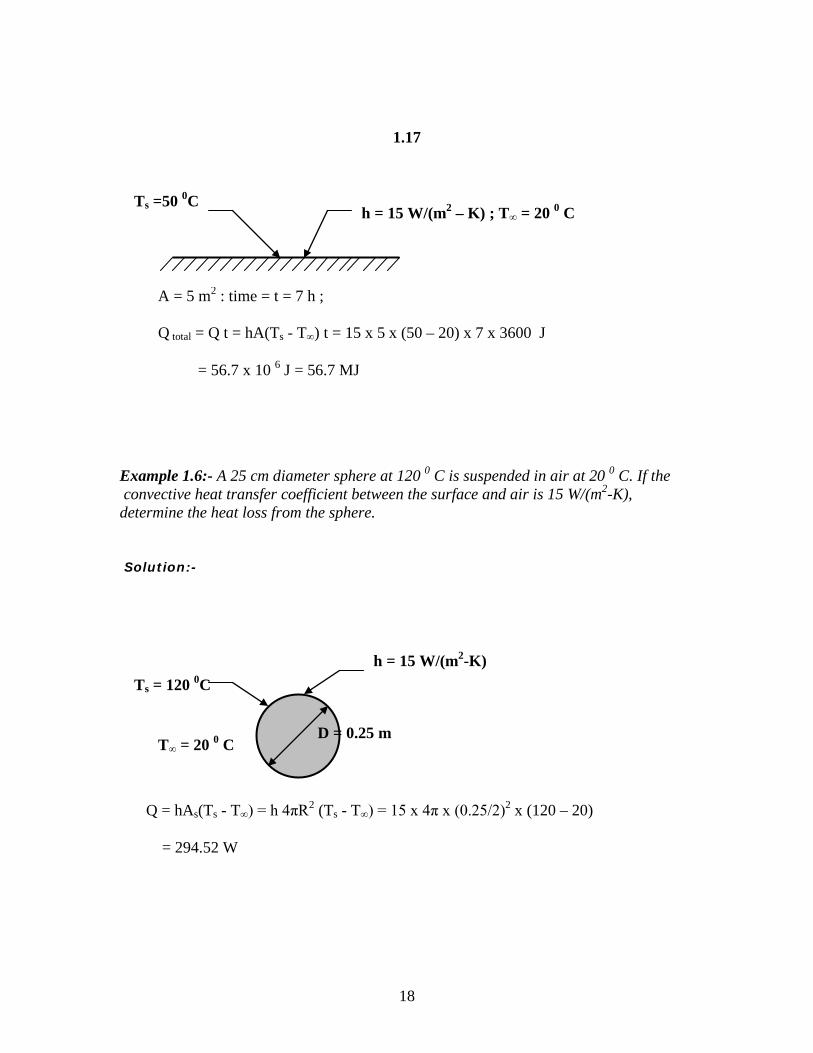
Example 1.6:- A 25 cm diameter sphere at 120 0 C is suspended in air at 20 0 C. If the convective heat transfer coefficient between the surface and air is 15 W/(m2-K), determine the heat loss from the sphere. Solution:-
Ts =50 0C h = 15 W/(m2 – K) ; T∞ = 20 0 C
A = 5 m2 : time = t = 7 h ; Q total = Q t = hA(Ts - T∞) t = 15 x 5 x (50 – 20) x 7 x 3600 J = 56.7 x 10 6 J = 56.7 MJ
D = 0.25 m
Ts = 120 0C
T∞ = 20 0 C
h = 15 W/(m2-K)
Q = hAs(Ts - T∞) = h 4πR2 (Ts - T∞) = 15 x 4π x (0.25/2)2 x (120 – 20) = 294.52 W

19
1.18 C. Radiation:
Example 1.7:- A sphere 10 cm in diameter is suspended inside a large evacuated chamber whose walls are kept at 300 K. If the surface of the sphere is black and maintained at 500 K what would be the radiation heat loss from the sphere to the walls of the chamber?. What would be the heat loss if the surface of the sphere has an emissivity of 0.8? Solution:
Example 1.8:- A vacuum system as used in sputtering conducting thin films on micro circuits, consists of a base plate maintained at a temperature of 300 K by an electric heater and a shroud within the enclosure maintained at 77 K by circulating liquid nitrogen. The base plate insulated on the lower side is 0.3 m in diameter and has an emissivity of 0.25. (a) How much electrical power must be provided to the base plate heater?
(b) At what rate must liquid nitrogen be supplied to the shroud if its latent heat of
vaporization is 125 kJ/kg?
Solution:- T1 = 300 K ; T2 = 77 K ; d = 0.3 m ; ε1 = 0.25 Surface area of the top surface of the base plate = As = (π / 4)d1
2 = (π / 4) x 0.32
T2
T1
d1
T1 = 500 K ; T2 = 300 K ; d1 = 0.10 m Surface area of the sphere = As
= 4πR12
= 4πx (0.1/2)2 = 0.0314 m2 If the surface of the sphere is black then Qblack = σ As (T1
4 – T24)
= 5.67 x 10 ─ 8x 0.0314 x (5004 – 3004) = 96.85 W If the surface is having an emissivity of 0.8 then Q = 0.8 Qblack = 0.8 x 96.85 = 77.48 W.

20
1.19 = 0.0707 m2 (a) Qr = ε1σ As (T1
4 – T24)
= 0.25 x 5.67 x 10 ─ 8 x 0.0707 x (3004 – 774) = 8.08 W . (b) If mN2 = mass flow rate of nitrogen that is vapourised then . 8.08 mN2 = Qr / hfg = ---------------- = 6.464 x 10⁻⁵ kg/s or 0.233 kg/s 125 x 1000
Example 1.9:- A flat plate has one surface insulated and the other surface exposed to the sun. The exposed surface absorbs the solar radiation at a rate of 800 W/m2 and dissipates heat by both convection and radiation into the ambient at 300 K. If the emissivity of the surface is 0.9 and the surface heat transfer coefficient is 12 W/(m2-K), determine the surface temperature of the plate. Solution:-
On simplifying the above equation we get (Ts / 100)4 + 2.35 Ts = 943 …………………………(1) Equation (1) has to be solved by trial and error.
Insulated
Qsolar
Qr
Qconv Ts ; ε = 0.9 ; h = 12 W / (m2 – K)
T∞ = 300 K ; qsolar = 800 W / m2
Energy balance equation for the top surface of the plate is given by Qsolar = Qr + Qconv qsolar As = ε σ As (Ts
4 - T∞4) + h As (Ts - T∞)
Therefore 800 = 0.9 x 5.67 x 10 ─ 8x (Ts
4 – 3004) + 12 x (Ts – 300)

21
1.20
Trial 1:- Assume Ts = 350 K. Then LHS of Eq. (1) = 972.6 which is more than RHS of Eq.(1). Hence Ts < 350 K. Trial 2 :- Assume Ts = 340 K. Then LHS of Eq. (1) = 932.6 which is slightly less than RHS. Therefore Ts should lie between 340 K and 350 K but closer to 340 K. Trial 3:- Assume Ts = 342.5 K. Then LHS of Eq.(1) = 942.5 = RHS of Eq. (1). Therefore Ts = 342.5 K Example 1.10:- The solar radiation incident on the outside surface of an aluminum shading device is 1000 W/m2. Aluminum absorbs 12 % of the incident solar energy and dissipates it by convection from the back surface and by combined convection and radiation from the outer surface. The emissivity of aluminum is 0.10 and the convective heat transfer coefficient for both the surfaces is 15 W/(m2 –K). The ambient temperature of air may be taken as 20 0 C. Determine the temperature of the shading device.
Solution:- qsolar = 1000 W / m2 ; absorptivity of aluminum = α = 0.12 ; emissivity of aluminum = ε = 0.10 ; h = 15 W /(m2 – K) ; T∞ = 20 + 273 = 293 K ; Solar radiation flux absorbed by aluminum = qa = α qsolar = 0.12 x 1000 = 120 W / m2.
q solar qr qc1
qc2
Therefore, qa = ε σ Ts4 – α σT∞
4) + h1(Ts - T∞) + h2 (Ts - T∞) Or 120 = 5.67 x 10 ─ 8x (0.10Ts
4 – 0.12 x 2934) + (Ts – 293)x (15 + 15) On simplifying we get, (Ts / 100)4 + 53 Ts = 15873 …………………………(1)
The energy absorbed by aluminum is dissipated by convection from the back surface and by combined convection and radiation from the outer surface. Hence the energy balance equation can be written as qa = qr + qc1 + qc2
22
1.21 Eq.(1) has to be solved by trial and error. Trail 1:- Assume Ts = 300 K. Then LHS = 15981 which is > RHS. Trail 2 :- Assume Ts = 295 K. Then LHS = 15710.73 which is < RHS. Hence Ts should lie between 300K and 295 K. Trial 3 :- Assume Ts = 297 K . Then LHS = 15819 which is almost equal to RHS (Within 0.34 %) Therefore Ts = 297 K. .

23
CHAPTER 2
GOVERNING EQUATIONS OF CONDUCTION
2.1.Introduction: In this chapter, the governing basic equations for conduction in Cartesian coordinate system is derived. The corresponding equations in cylindrical and spherical coordinate systems are also mentioned. Mathematical representations of different types of boundary conditions and the initial condition required to solve conduction problems are also discussed. After studying this chapter, the student will be able to write down the governing equation and the required boundary conditions and initial condition if required for any conduction problem. 2.2. One – Dimensional Conduction Equation : In order to derive the one-dimensional conduction equation, let us consider a volume element of the solid of thickness Δx along x – direction at a distance ‘x’ from the origin as shown in Fig. 2.1.Qx represents the rate
of heat transfer in x – direction entering into the volume element at x, A(x) area of heat flow at the section x ,q’’’ is the thermal energy generation within the element per unit volume and Qx+Δx is the rate of conduction out of the element at the section x + Δx. The energy balance equation per unit time for the element can be written as follows:
x
Qx Qx + Δx
q’’’
Fig. 2.1: Nomenclature for one dimensional conduction equation
O
A(x)

24
2.2 [ Rate of heat conduction into the element at x + Rate of thermal energy generation within the element − Rate of heat conduction out of the element at x + Δx ] = Rate of increase of internal energy of the element. i.e., Qx + Qg – Qx+Δx = ∂E / ∂t or Qx + q’’’ A(x) Δx – {Qx + (∂Qx / ∂x)Δx + (∂2Qx / ∂x2)(Δx)2 / 2! + …….} = ∂/ ∂t (ρA(x)ΔxCpT) Neglecting higher order terms and noting that ρ and Cp are constants the above equation simplifies to Qx + q’’’ A(x) Δx – {Qx + (∂Qx / ∂x)Δx = ρA(x)ΔxCp (∂T/ ∂t) Or − (∂Qx / ∂x) + q’’’ A(x) = ρA(x) Cp (∂T/ ∂t) Using Fourier’s law of conduction , Qx = − k A(x) (∂T / ∂x), the above equation simplifies to − ∂/ ∂x {− k A(x) (∂T / ∂x)} + q’’’ A(x) = ρA(x) Cp (∂T/ ∂t) Or {1/A(x)} ∂/ ∂x {k A(x) (∂T / ∂x)} + q’’’ = ρ Cp (∂T/ ∂t) ……………(2.1) Eq. (2.1) is the most general form of conduction equation for one-dimensional unsteady state conduction. 2.2.1.Equation for one-dimensional conduction in plane walls :- For plane walls, the area of heat flow A(x) is a constant. Hence Eq. (2.1) reduces to the form ∂/ ∂x {k (∂T / ∂x)} + q’’’ = ρ Cp (∂T/ ∂t) …………………(2.2) (i) If the thermal conductivity of the solid is constant then the above equation reduces to (∂2T / ∂x2) + (q’’’ / k) = (1/α )(∂T/ ∂t) ………………………(2.3) (ii) For steady state conduction problems in solids of constant thermal conductivity temperature within the solid will be independent of time (i.e.(∂T/ ∂t) = 0) and hence Eq. (2.3) reduces to (d2T / dx2 )+ (q’’’ / k) = 0………………………………….(2.4)

25
2.3 (iii) For a solid of constant thermal conductivity for which there is no thermal energy generation within the solid q’’’ = 0 and the governing for steady state conduction is obtained by putting q’’’ = 0 in Eq. (2.4) as (d2T / dx2 ) = 0 ………………………………(2.4) 2.2.2.Equation for one-dimensional radial conduction in cylinders:-
. For radial conduction in cylinders, by convention the radial coordinate is denoted by ‘r’ instead of ‘x’ and the area of heat flow through the cylinder of length L,at any radius r is given by A(x) = A(r) = 2πrL. Hence substituting this expression for A(x) and replacing x by r in Eq. (2.1) we have {1/(2πrL)∂/ ∂r {k 2πrL (∂T / ∂r)} + q’’’ = ρ Cp (∂T/∂t) Or (1/r) ∂/ ∂r {k r (∂T / ∂r)} + q’’’ = ρ Cp (∂T/ ∂t)…………….(2.5) (i) For cylinders of constant thermal conductivity the above equation reduces to (1/r) ∂/ ∂r { r (∂T / ∂r)} + q’’’ / k = (1 / α) (∂T/ ∂t)…………….(2.6)
R Qr
L
r
Qr

26
2.4 (ii) For steady state radial conduction (i.e. (∂T/ ∂t) = 0 ) in cylinders of constant k, the above equation reduces to (1/r) d/ dr { r (dT / ∂r)} + q’’’ / k = 0 ………………………….(2.7) (iii) For steady state radial conduction in cylinders of constant k and having no thermal energy generation (i.e. q’’’ = 0) the above equation reduces to d/ dr { r (dT / ∂r)} = 0 ………………………………(2.8) 2.2.3.Equation for one-dimensional radial conduction in spheres:- For one-dimensional radial conduction in spheres, the area of heat flow at any radius r is given by A(r) = 4πr2. Hence Eq.(2.1) for a sphere reduces to {1/(4π r2 )}∂/ ∂r {k 4π r2 (∂T / ∂r)} + q’’’ = ρCp (∂T/ ∂t) Or 1/r2 ∂/ ∂r {k r2 (∂T / ∂r)} + q’’’ = ρ Cp (∂T/ ∂t) …………………(2.9) (i) For spheres of constant thermal conductivity the above equation reduce to 1/r2 ∂/ ∂r { r2 (∂T / ∂r)} + q’’’ / k = (1 / α) (∂T/ ∂t) ……………..(2.10) (ii) For steady state conduction in spheres of constant k the above equation further reduce to 1/r2 ∂/ ∂r { r2 (∂T / ∂r)} + q’’’ / k = 0 ……………………………(2.11) (iii) For steady state conduction in spheres of constant k and without any thermal energy generation the above equation further reduces to 1/r2 d/ dr { r2 (dT / dr)} = 0 ……………………………………(2.12) Equation in compact form:- The general form of one – dimensional conduction equations for plane walls, cylinders and spheres {equations (2..2), (2.5) and (2.9)} can be written in a compact form as follows: 1/rn ∂/ ∂r {k rn (∂T / ∂r)} + q’’’ = ρ Cp (∂T/ ∂t) ………….(2.13) Where n = 0 for plane walls, n = 1 for radial conduction in cylinders n = 2 for radial conduction in spheres, and for plane walls it is customary to replace the ‘r’ variable by ‘x’ variable.

27
2.5
2.3.Three dimensional conduction equations: While deriving the one – dimensional conduction equation, we assumed that conduction heat transfer is taking place only along one direction. By allowing conduction along the remaining two directions and following the same procedure we obtain the governing equation for conduction in three dimenions. 2.3.1. Three dimensional conduction equation in Cartesian coordinate system: Let us consider a volume element of dimensions Δx, Δy and Δz in x y and z directions respectively. The conduction heat transfer across the six surfaces of the element is shown in Fig. 2.3.
Net Rate of conduction into the element in x-direction = Qx – Qx + Δx = Qx – [Qx + (∂Qx/∂x) Δx + (∂2Qx/∂x2)(Δx)2 / 2! + ….] = − (∂Qx/∂x) Δx by neglecting higher order terms. = − ∂ / ∂x [− kx Δy Δz(∂T / ∂x)] Δx = ∂ / ∂x[kx (∂T / ∂x)] Δx Δy Δz Similarly the net rate of conduction into the element in y – direction = ∂ / ∂y[ky (∂T / ∂y)] Δx Δy Δz and in z – direction = ∂ / ∂z[kz (∂T / ∂z)] Δx Δy Δz.
Δx
Δy
Δz
Qx Qx + Δx
Qz Qy
x
y z
Fig. 2.3: Conduction heat transfer across the six faces of a volume element
Qz + Δz Qy + Δy

28
2.6 Hence the net rate of conduction into the element from all the three directions Qin = {∂ / ∂x[kx (∂T / ∂x)] + ∂ / ∂y[ky (∂T / ∂y)] + ∂ / ∂z[kz (∂T / ∂z)] } Δx Δy Δz Rate of heat thermal energy generation in the element = Qg = q’’’ Δx Δy Δz Rate of increase of internal energy within the element = ∂E / ∂t = ρ Δx Δy Δz Cp (∂T / ∂t) Applying I law of thermodynamics for the volume element we have Qin + Qg = ∂E / ∂t Substituting the expressions for Qin, Qg and ∂E / ∂t and simplifying we get {∂ / ∂x[kx (∂T / ∂x)] + ∂ / ∂y[ky (∂T / ∂y)] + ∂ / ∂z[kz (∂T / ∂z)] } + q’’’ = ρ Cp (∂T / ∂t) ……………………(2.14) Equation (2.14) is the most general form of conduction equation in Cartesian coordinate system. This equation reduces to much simpler form for many special cases as indicated below. Special cases:- (i) For isotropic solids, thermal conductivity is independent of direction; i.e., kx = ky = kz = k. Hence Eq. (2.14) reduces to {∂ / ∂x[k (∂T / ∂x)] + ∂ / ∂y[k (∂T / ∂y)] + ∂ / ∂z[k (∂T / ∂z)] } + q’’’ = ρ Cp (∂T / ∂t) ……………………..(2.15) (ii) For isotropic solids with constant thermal conductivity the above equation further reduces to ∂2T / ∂x2 + ∂2T / ∂y2 + ∂2T / ∂z2 + q’’’ / k = (1 / α) (∂T / ∂t)…………………….(2.16) Eq.(2.16) is called as the “Fourier – Biot equation” and it reduces to the following forms under specified conditions as mentioned below: (iii) Steady state conduction [i.e., (∂T / ∂t) = 0] ∂2T / ∂x2 + ∂2T / ∂y2 + ∂2T / ∂z2 + q’’’ / k = 0 …………………………….(2.17) Eq. (2.17) is called the “Poisson equation”. (iv) No thermal energy generation [i.e. q’’’ = 0]: ∂2T / ∂x2 + ∂2T / ∂y2 + ∂2T / ∂z2 = (1 / α) (∂T / ∂t)……………………………..(2.18)
29
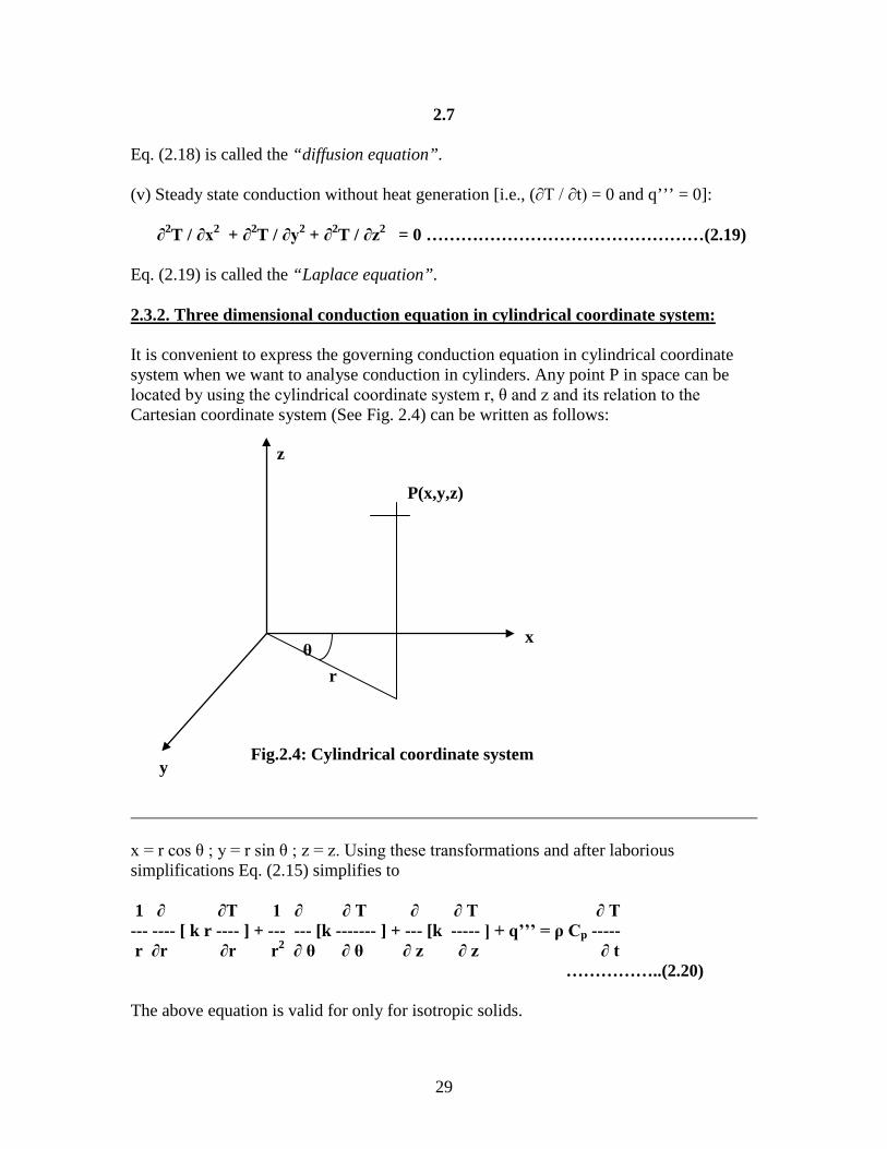
2.7 Eq. (2.18) is called the “diffusion equation”. (v) Steady state conduction without heat generation [i.e., (∂T / ∂t) = 0 and q’’’ = 0]: ∂2T / ∂x2 + ∂2T / ∂y2 + ∂2T / ∂z2 = 0 …………………………………………(2.19) Eq. (2.19) is called the “Laplace equation”. 2.3.2. Three dimensional conduction equation in cylindrical coordinate system: It is convenient to express the governing conduction equation in cylindrical coordinate system when we want to analyse conduction in cylinders. Any point P in space can be located by using the cylindrical coordinate system r, θ and z and its relation to the Cartesian coordinate system (See Fig. 2.4) can be written as follows:
x = r cos θ ; y = r sin θ ; z = z. Using these transformations and after laborious simplifications Eq. (2.15) simplifies to 1 ∂ ∂T 1 ∂ ∂ T ∂ ∂ T ∂ T --- ---- [ k r ---- ] + --- --- [k ------- ] + --- [k ----- ] + q’’’ = ρ Cp ----- r ∂r ∂r r2 ∂ θ ∂ θ ∂ z ∂ z ∂ t ……………..(2.20) The above equation is valid for only for isotropic solids.
r θ
x
y
z
P(x,y,z)
Fig.2.4: Cylindrical coordinate system
30
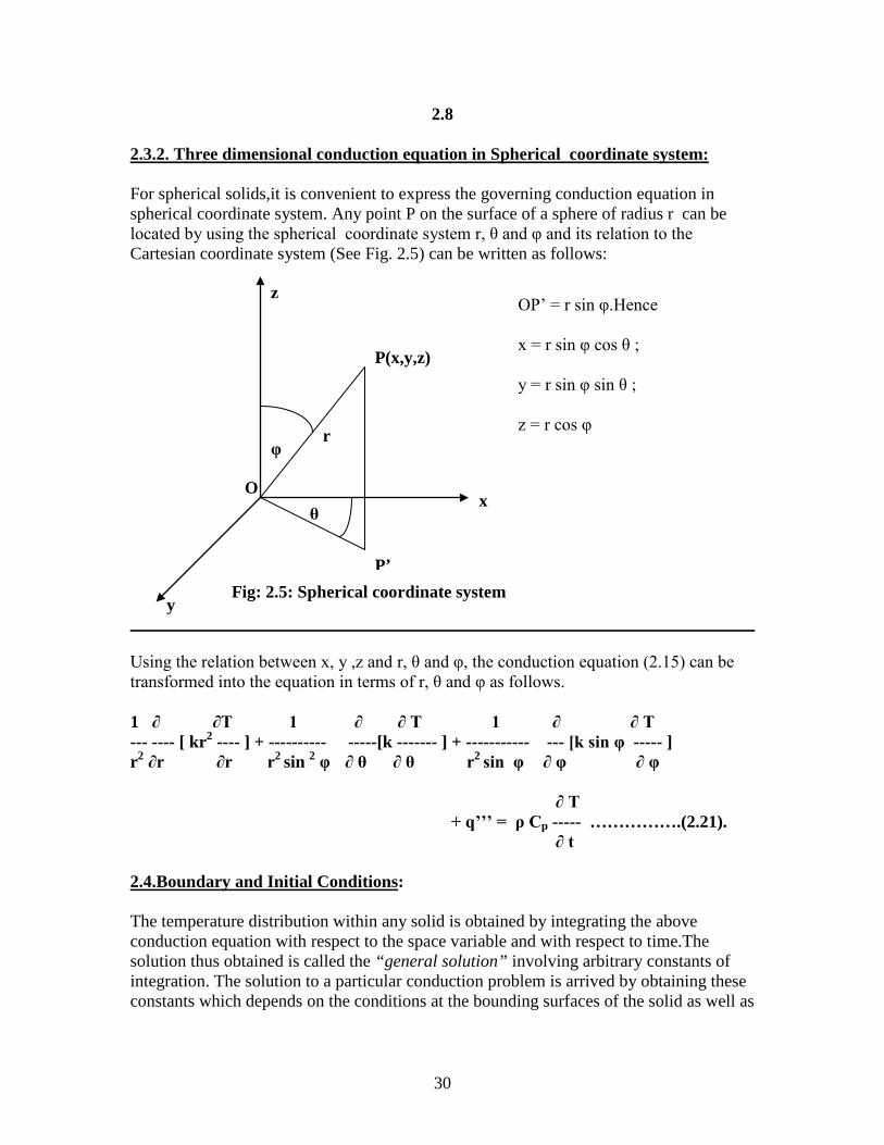
2.8 2.3.2. Three dimensional conduction equation in Spherical coordinate system: For spherical solids,it is convenient to express the governing conduction equation in spherical coordinate system. Any point P on the surface of a sphere of radius r can be located by using the spherical coordinate system r, θ and φ and its relation to the Cartesian coordinate system (See Fig. 2.5) can be written as follows:
Using the relation between x, y ,z and r, θ and φ, the conduction equation (2.15) can be transformed into the equation in terms of r, θ and φ as follows. 1 ∂ ∂T 1 ∂ ∂ T 1 ∂ ∂ T --- ---- [ kr2 ---- ] + ---------- -----[k ------- ] + ----------- --- [k sin φ ----- ] r2 ∂r ∂r r2 sin 2 φ ∂ θ ∂ θ r2 sin φ ∂ φ ∂ φ ∂ T + q’’’ = ρ Cp ----- …………….(2.21). ∂ t 2.4.Boundary and Initial Conditions: The temperature distribution within any solid is obtained by integrating the above conduction equation with respect to the space variable and with respect to time.The solution thus obtained is called the “general solution” involving arbitrary constants of integration. The solution to a particular conduction problem is arrived by obtaining these constants which depends on the conditions at the bounding surfaces of the solid as well as
P(x,y,z)
r φ
x
y
z
θ
Fig: 2.5: Spherical coordinate system P’
O
OP’ = r sin φ.Hence x = r sin φ cos θ ; y = r sin φ sin θ ; z = r cos φ

31
2.9 the initial condition. The thermal conditions at the boundary surfaces are called the “boundary conditions” . Boundary conditions normally encountered in practice are: (i) Specified temperature (also called as boundary condition of the first kind), (ii) Specified heat flux (also known as boundary condition of the second kind), (iii) Convective boundary condition (also known as boundary condition of the third kind) and (iv) radiation boundary condition. The mathematical representations of these boundary conditions are illustrated by means of a few examples below. 2.4.1. Specified Temperatures at the Boundary:- Consider a plane wall of thickness L whose outer surfaces are maintained at temperatures T0 and TL as shown in Fig.2.6. For one-dimensional unsteady state conduction the boundary conditions can be written as
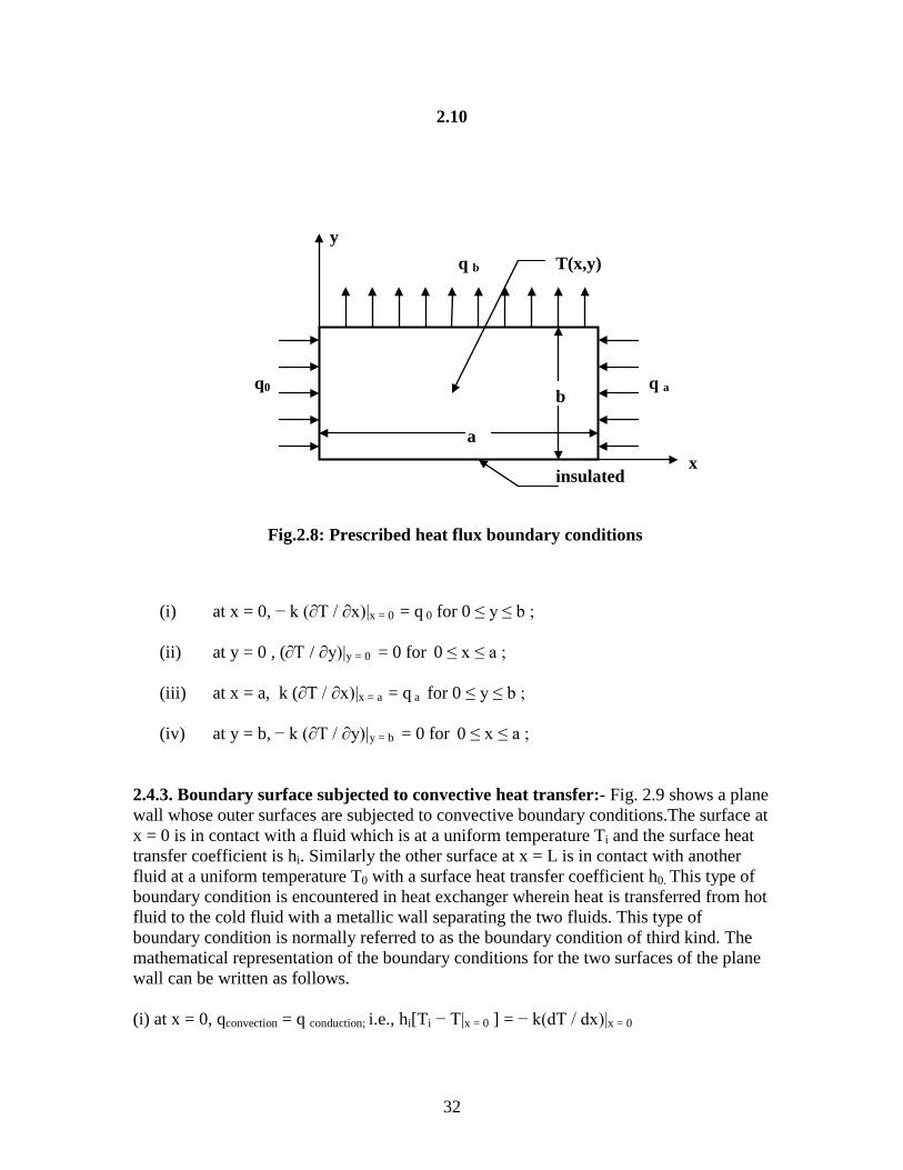
(i) at x = 0, T(0,t) = T0 ; (ii) at x = L, T(L,t) = TL. Consider another example of a rectangular plate as shown in Fig. 2.7. The boundary conditions for the four surfaces to determine two-dimensional steady state temperature distribution T(x,y) can be written as follows. (i) at x = 0, T(0,y) = Ψ(y) ; (ii) at y = 0, T(x,0) = T1 for all values of y (iii) at x = a, T(a,y) = T2 for all values of y; (iv) at y = b, T(x,b) = φ(x) 2.4.2. Specified heat flux at the boundary:- Consider a rectangular plate as shown in Fig. 2.8 and whose boundaries are subjected to the prescribed heat flux conditions as shown in the figure. Then the boundary conditions can be mathematically expressed as follows.
x
L
TL T0
T(x,t)
Fig. 2.6: Boundary condition Fig.2.7: Boundary conditions of of first kind for a plane wall first kind for a rectangular plate
x
y
a
b
T = φ(x)
T1
Ψ(y)
T2
T(x,y)
32
2.10
(i) at x = 0, − k (∂T / ∂x)|x = 0 = q 0 for 0 ≤ y ≤ b ; (ii) at y = 0 , (∂T / ∂y)|y = 0 = 0 for 0 ≤ x ≤ a ;
(iii) at x = a, k (∂T / ∂x)|x = a = q a for 0 ≤ y ≤ b ;
(iv) at y = b, − k (∂T / ∂y)|y = b = 0 for 0 ≤ x ≤ a ;
2.4.3. Boundary surface subjected to convective heat transfer:- Fig. 2.9 shows a plane wall whose outer surfaces are subjected to convective boundary conditions.The surface at x = 0 is in contact with a fluid which is at a uniform temperature Ti and the surface heat transfer coefficient is hi. Similarly the other surface at x = L is in contact with another fluid at a uniform temperature T0 with a surface heat transfer coefficient h0. This type of boundary condition is encountered in heat exchanger wherein heat is transferred from hot fluid to the cold fluid with a metallic wall separating the two fluids. This type of boundary condition is normally referred to as the boundary condition of third kind. The mathematical representation of the boundary conditions for the two surfaces of the plane wall can be written as follows. (i) at x = 0, qconvection = q conduction; i.e., hi[Ti − T|x = 0 ] = − k(dT / dx)|x = 0
a
b
x
y
q0 q a
q b
insulated
T(x,y)
Fig.2.8: Prescribed heat flux boundary conditions

33
2.11 (ii) at x = L, − k(dT / dx)|x = L = h0 [T|x = L − T0]
2.4.4.Radiation Boundary Condition:Fig. 2.10 shows a plane wall whose surface at x =L is having an emissivity ‘ε’ and is radiating heat to the surroundings at a uniform temperature Ts. The mathematical expression for the boundary condition at x = L can be written as follows:
(i) at x = L, qconduction = qradiation ; i.e., − k (dT / dx)| x = L = σ ε [( T| x = L)4 − Ts 4]
x
L
T(x)
Fig. 2.9: Boundaries subjected to convective heat transfer for a plane wall
Surface in contact with fluid at T0 with surface heat transfer coefficient h0
Surface in contact with fluid at Ti with surface heat transfer coefficient h i
x
L
T(x,t)
Fig. 2.10: Boundary surface at x = L subjected to radiation heat transfer
Surface with emissivity ε is radiating heat to the surroundings at Ts 0K

34
2.12
In the above equation both T| x = L and Ts should be expressed in degrees Kelvin. 2.4.5. General form of boundary condition (combined conduction, convection and radiation boundary condition): There are situations where the boundary surface is subjected to combined conduction, convection and radiation conditions as illustrated in Fig. 2.11.It is a south wall of a house and the outer surface of the wall is exposed to solar radiation. The interior of the room is at a uniform temperature Ti. The outer air is at uniform temperature T0 . The sky, the ground and the surfaces of the surrounding structures at this location is modeled as a surface at an effective temperature of Tsky.
Energy balance for the outer surface is given by the equation qconduction + α qsolar = qradiation + qconvection
− k (dT / dx)|x = L + αqsolar = ε σ [(T|x = L)4 − Tsky
4] + h0[T|x = L − T0]
qradiation
αqsolar
qconvection
qconduction
Fig. 2.11: Schematic for general form of boundary condition
x L

35
2.13 2.5. Illustrative Examples: A. Derivation of conduction Equations: 2.1. By writing an energy balance for a differential cylindrical volume element in
the ‘r’ variable (r is any radius), derive the one-dimensional time dependent heat conduction equation with internal heat generation and variable thermal conductivity in the cylindrical coordinate system.
2.2. By writing an energy balance for a differential spherical volume element in
the ‘r’ variable (r is any radius), derive the one-dimensional time dependent heat conduction equation with internal heat generation and variable thermal conductivity in the spherical coordinate system.
2.3. By simplifying the three-dimensional heat conduction equation, obtain one-
dimensional steady-state conduction equation with heat generation and constant thermal conductivity for the following coordinate systems:
(a) Rectangular coordinate in the ‘x’ variable. (b) Cylindrical coordinate in the r variable. (c) Spherical coordinates in the ‘r’ variable
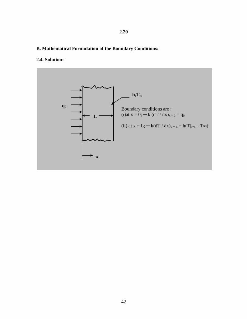
B. Mathematical Formulation of Boundary conditions: 2.4. A plane wall of thickness L is subjected to a heat supply at a rate of q0 W/m2
at one boundary surface and dissipates heat from the surface by convection to the ambient which is at a uniform temperature of T∞ with a surface heat transfer coefficient of h∞.Write the mathematical formulation of the boundary conditions for the plane wall.
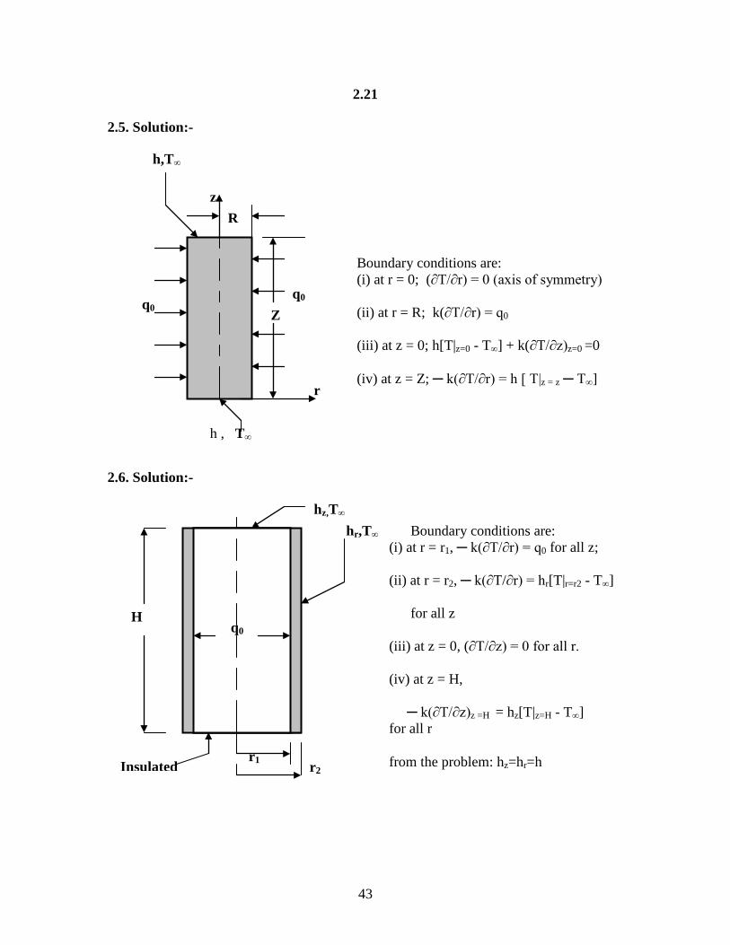
2.5. Consider a solid cylinder of radius R and height Z. The outer curved surface of
the cylinder is subjected to a uniform heating electrically at a rate of q0 W / m2.Both the circular surfaces of the cylinder are exposed to an environment at a uniform temeperature T∞ with a surface heat transfer coefficient h.Write the mathematical formulation of the boundary conditions for the solid cylinder.
2.6. A hollow cylinder of inner radius ri, outer radius r0 and height H is subjected
to the following boundary conditions. (a) The inner curved surface is heated uniformly with an electric heater at a
constant rate of q0 W/m2, (b) the outer curved surface dissipates heat by convection into an ambient at a
uniform temperature, T∞ with a convective heat transfer coefficient,h (c) the lower flat surface of the cylinder is insulated, and (d) the upper flat surface of the cylinder dissipates heat by convection into the
ambient at T∞ with surface heat transfer coefficient h. Write the mathematical formulation of the boundary conditions for the hollow cylinder.

36
2.14
C. Formulation of Heat Conduction Problems: 2.7. A plane wall of thickness L and with constant thermal properties is initially at
a uniform temperature Ti. Suddenly one of the surfaces of the wall is subjected to heating by the flow of a hot gas at temperature T∞ and the other surface is kept insulated. The heat transfer coefficient between the hot gas and the surface exposed to it is h. There is no heat generation in the wall. Write the mathematical formulation of the problem to determine the one-dimensional unsteady state temperature within the wall.
2.8. A copper bar of radius R is initially at a uniform temperature Ti. Suddenly the
heating of the rod begins at time t=0 by the passage of electric current, which generates heat at a uniform rate of q’’’ W/m2. The outer surface of the dissipates heat into an ambient at a uniform temperature T∞ with a convective heat transfer coefficient h. Assuming that thermal conductivity of the bar to be constant, write the mathematical formulation of the heat conduction problem to determine the one-dimensional radial unsteady state temperature distribution in the rod.
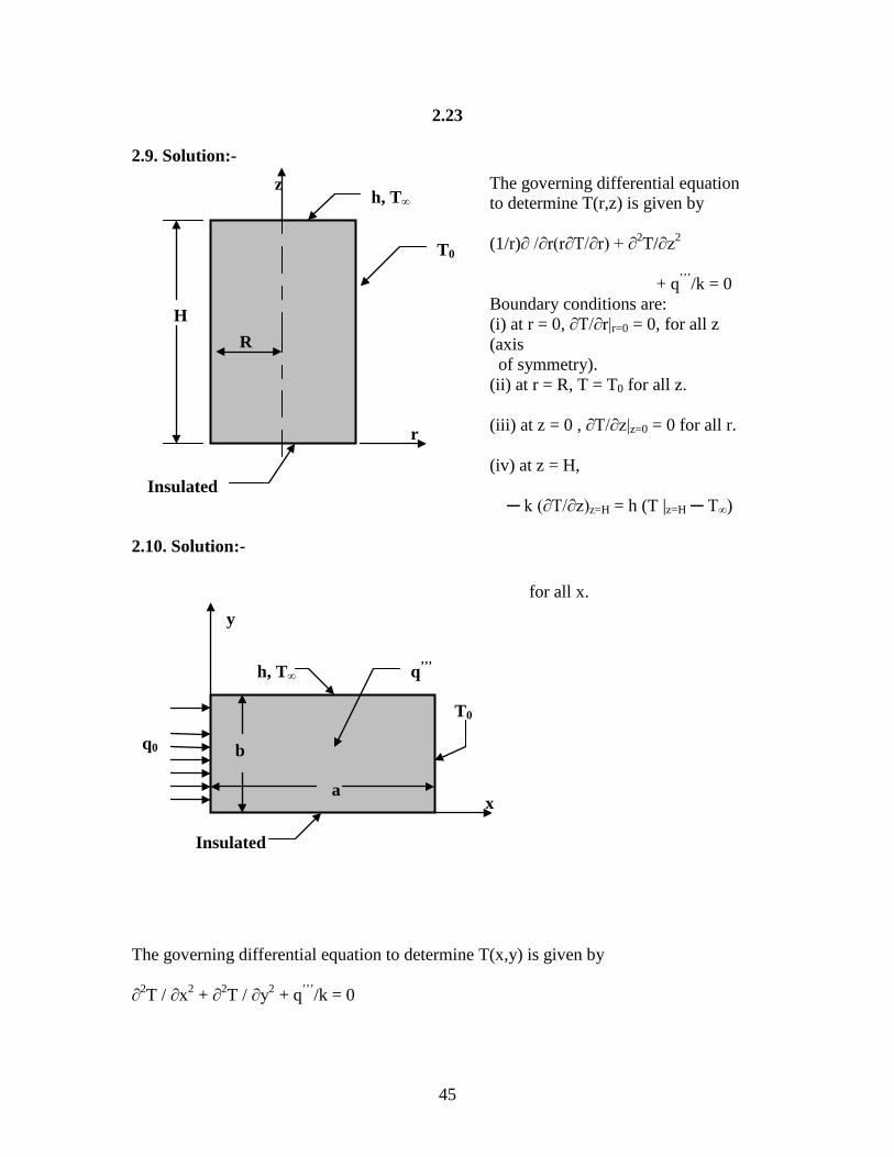
2.9. Consider a solid cylinder of radius R and height H. Heat is generated in the
solid at a uniform rate of q’’’ W/m3. One of the circular faces of the cylinder is insulated and the other circular face dissipates heat by convection into a medium at a uniform temperature of T∞ with a surface heat transfer coefficient of h. The outer curved surface of the cylinder is maintained at a uniform temperature of T0. Write the mathematical formulation to determine the two-dimensional steady state temperature distribution T(r,z) in the cylinder.
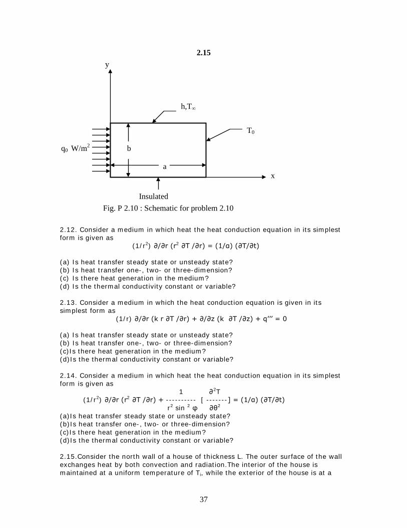
2.10. Consider a rectangular plate as shown in Fig. P2.10. The plate is generating
heat at a uniform rate of q’’’ W/m3. Write the mathematical formulation to determine two-dimensional steady state temperature distribution in the plate.
2.11. Consider a medium in which the heat conduction rquation is given in its simple form as ∂2T / ∂x2 = (1/α) (∂T / ∂t)
(a) Is heat transfer in this medium steady or transient? (b) Is heat transfer one-, two- or three-dimensional? (c) Is there heat generation in the medium? (d) Is thermal conductivity of the medium constant or variable?
2.11. Consider a medium in which the heat conduction equation is given in its simple form as (1/r) d / dr(r k dT/dr) + q’’’ = 0.
(a) Is heat transfer steady or unsteady? (b) Is heat transfer one-, two- or three-dimensional? (c) Is there heat generation in the medium? (d) Is the thermal conductivity of the medium constant or variable?
37
2.15
2.12. Consider a medium in which heat the heat conduction equation in its simplest form is given as (1/r2) ∂/∂r (r2 ∂T /∂r) = (1/α) (∂T/∂t) (a) Is heat transfer steady state or unsteady state? (b) Is heat transfer one-, two- or three-dimension? (c) Is there heat generation in the medium? (d) Is the thermal conductivity constant or variable? 2.13. Consider a medium in which the heat conduction equation is given in its simplest form as (1/r) ∂/∂r (k r ∂T /∂r) + ∂/∂z (k ∂T /∂z) + q’’’ = 0 (a) Is heat transfer steady state or unsteady state? (b) Is heat transfer one-, two- or three-dimension? (c)Is there heat generation in the medium? (d)Is the thermal conductivity constant or variable? 2.14. Consider a medium in which heat the heat conduction equation in its simplest form is given as 1 ∂2T (1/r2) ∂/∂r (r2 ∂T /∂r) + ---------- [ -------] = (1/α) (∂T/∂t) r2 sin 2 φ ∂θ2
(a)Is heat transfer steady state or unsteady state? (b)Is heat transfer one-, two- or three-dimension? (c)Is there heat generation in the medium? (d)Is the thermal conductivity constant or variable? 2.15.Consider the north wall of a house of thickness L. The outer surface of the wall exchanges heat by both convection and radiation.The interior of the house is maintained at a uniform temperature of Ti, while the exterior of the house is at a
x
T0
Insulated
h,T∞
a b b
a
Fig. P 2.10 : Schematic for problem 2.10
y
q0 W/m2
38
2.16 uniform temperature T0. The sky, the ground, and the surfaces of the surrounding structures at this location can be modeled as a surface at an effective temperature of Tsky for radiation heat exchange on the outer surface.The radiation heat exchange between the inner surface of the wall and the surfaces of the other walls, floor and ceiling are negligible.The convective heat transfer coefficient for the inner and outer surfaces of the wall under consideration are hi and h0 respectively.The thermal conductivity of the wall material is K and the emissivity of the outer surface of the wall is ‘ε0’. Assuming the heat transfer through the wall is steady and one dimensional, express the mathematical formulation (differential equation and boundary conditions) of the heat conduction problem
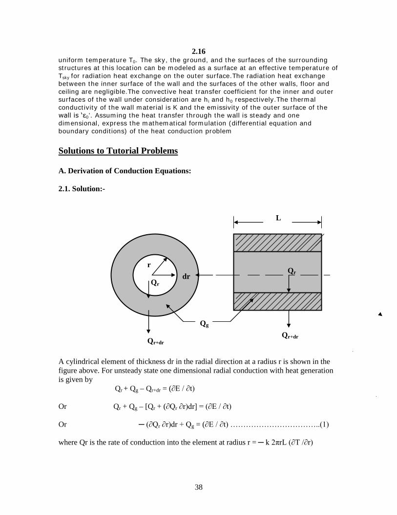
Solutions to Tutorial Problems A. Derivation of Conduction Equations: 2.1. Solution:-
A cylindrical element of thickness dr in the radial direction at a radius r is shown in the figure above. For unsteady state one dimensional radial conduction with heat generation is given by Qr + Qg – Qr+dr = (∂E / ∂t) Or Qr + Qg – [Qr + (∂Qr ∂r)dr] = (∂E / ∂t) Or ─ (∂Qr ∂r)dr + Qg = (∂E / ∂t) ……………………………..(1) where Qr is the rate of conduction into the element at radius r = ─ k 2πrL (∂T /∂r)
dr r
Qr+dr
Qr
Qg
Qr+dr
Qr
L
39
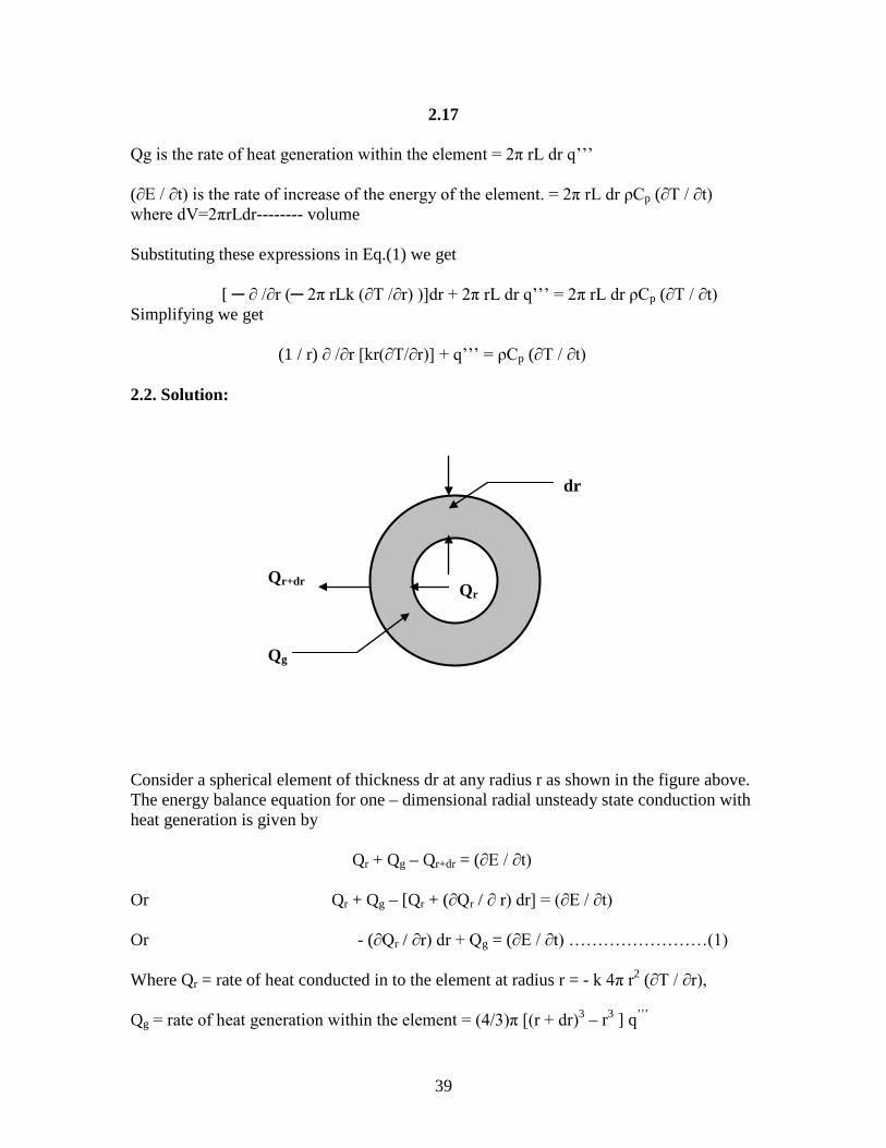
2.17 Qg is the rate of heat generation within the element = 2π rL dr q’’’ (∂E / ∂t) is the rate of increase of the energy of the element. = 2π rL dr ρCp (∂T / ∂t) where dV=2πrLdr-------- volume Substituting these expressions in Eq.(1) we get [ ─ ∂ /∂r (─ 2π rLk (∂T /∂r) )]dr + 2π rL dr q’’’ = 2π rL dr ρCp (∂T / ∂t) Simplifying we get (1 / r) ∂ /∂r [kr(∂T/∂r)] + q’’’ = ρCp (∂T / ∂t) 2.2. Solution:
Consider a spherical element of thickness dr at any radius r as shown in the figure above. The energy balance equation for one – dimensional radial unsteady state conduction with heat generation is given by Qr + Qg – Qr+dr = (∂E / ∂t) Or Qr + Qg – [Qr + (∂Qr / ∂ r) dr] = (∂E / ∂t) Or - (∂Qr / ∂r) dr + Qg = (∂E / ∂t) ……………………(1) Where Qr = rate of heat conducted in to the element at radius r = - k 4π r2 (∂T / ∂r), Qg = rate of heat generation within the element = (4/3)π [(r + dr)3 – r3 ] q’’’
Qr Qr+dr
Qg
dr

40
2.18 (∂E / ∂t) = rate of increase of energy of the element = ρ (4/3)π [ (r + dr) 3 – r3 ](∂T/∂t) Now (r + dr)3 – r3 = r3 + 3r2dr + 3r(dr)2 + (dr)3 – r3 = 3r2dr + 3r(dr)2 + (dr)3 Neglecting higher order terms like (dr)3 and (dr)2 we have (r + dr)3 – r3 = 3 r2 dr. Therefore Qg = 4 π r2 dr q’’’ And (∂E / ∂t) = ρ 4 π r2 dr Cp(∂T/∂t). Substituting the expressions for Qr, Qg and (∂E / ∂t) in Eq. (1) we have ─ [∂ /∂r{- k 4π r2 (∂T / ∂r)}]dr + 4 π r2 dr q’’’ = ρ 4 π r2 dr Cp(∂T/∂t) Simplifying the above equation and noting that if k is given to be constant we have ∂ /∂r{ r2 (∂T / ∂r)} + r2 ( q’’’/ k) = (ρ r2 Cp / k)(∂T/∂t) Or (1 / r2) ∂ /∂r{ r2 (∂T / ∂r)} + ( q’’’/ k) = (1 / α) (∂T/∂t); where α = k / (ρ Cp) 2.3. Solution:- (a) The general form of conduction equation for an isotropic solid in rectangular coordinate system is given by ∂ / ∂x (k∂T / ∂x) + ∂ / ∂y (k∂T / ∂y) + ∂ / ∂z (k∂T / ∂z) + q’’’ = (ρ Cp) (∂T / ∂t) …………..(1) For steady state conduction (∂T / ∂t) = 0 ; For one dimensional conduction in x – direction we have ∂T / ∂y = ∂T / ∂z = 0 . Therefore ∂T / ∂x = dT / dx . Therefore Eq. (1) reduces to d / dx (k dT / dx) + q’’’ = 0. For constant thermal conductivity the above equation reduces to d2 T / dx2 + q’’’/ k = 0. (b) The general form of conduction equation in cylindrical coordinate system is given by (1 / r) ∂ / ∂r (kr ∂T / ∂r) + (1 / r2) ∂ / ∂θ(k ∂T / ∂θ) + ∂ / ∂z (k∂T / ∂z) + q’’’ = ρCp( ∂T / ∂t)

41
2.19 For steady state conduction, ( ∂T / ∂t) = 0 ; For one-dimensional radial conduction we have ∂T / ∂θ = 0 and ∂T / ∂z = 0. Therefore ∂T / ∂r = dT / dr. With these simplifications the general form of conduction equation reduces to (1 / r) d / dr (kr dT/dr) + q’’’ = 0
For constant thermal conductivity the above equation reduces to (1 / r) d / dr (r dT/dr) + q’’’/ k = 0. © The general form of conduction equation in spherical coordinate system is given by (1/r2) ∂ / ∂r(kr2 ∂T / ∂r) + {1/(r2 sin 2 φ)}∂ / ∂θ (k ∂T/∂θ) + {1/(r2 sin φ)} ∂ /∂φ (k sin φ ∂T/∂φ) + q’’’ = ρCp (∂T/ ∂t) ………..(1) For steady state conduction (∂T ∂t) = 0 ; For one dimensional radial conduction we have ∂T/∂θ = 0 and ∂T/∂φ = 0. Therefore ∂T / ∂r = dT / dr. Substituting these conditions in Eq. (1) we have (1/r2) d / dr (kr2 dT / dr) + q’’’ = 0. For constant thermal conductivity the above equation reduces to (1/r2) d / dr (r2 dT / dr) + q’’’ / k = 0.
42
2.20 B. Mathematical Formulation of the Boundary Conditions: 2.4. Solution:-
h,T∞
q0
L Boundary conditions are : (i)at x = 0; ─ k (dT / dx)x = 0 = q0
(ii) at x = L; ─ k(dT / dx)x = L = h(T|x=L - T∞)
x
43
2.21 2.5. Solution:-
2.6. Solution:-
z
r
Z
R
q0
h , T∞
q0
Boundary conditions are: (i) at r = 0; (∂T/∂r) = 0 (axis of symmetry) (ii) at r = R; k(∂T/∂r) = q0 (iii) at z = 0; h[T|z=0 - T∞] + k(∂T/∂z)z=0 =0 (iv) at z = Z; ─ k(∂T/∂r) = h [ T|z = z ─ T∞]
r1
H q0
Insulated
hz,T∞
hr,T∞
Boundary conditions are: (i) at r = r1, ─ k(∂T/∂r) = q0 for all z; (ii) at r = r2, ─ k(∂T/∂r) = hr[T|r=r2 - T∞] for all z (iii) at z = 0, (∂T/∂z) = 0 for all r. (iv) at z = H, ─ k(∂T/∂z)z =H = hz[T|z=H - T∞] for all r from the problem: hz=hr=h r2
q0
h,T∞

44
2.22 C. Mathematical Formulation of Conduction Problems: 2.7. Solution:-
2.8. Solution:-
L Insulated h∞,T∞ T =
T(x,t)
T = Ti at t = 0
Governing differential equation to determine T(x,t) is given by (∂ 2T / ∂ x2) = (1 / α) (∂T / ∂t) where α is the thermal diffusivity of the wall. Initial condition is at time t = 0 T = Ti for all x.
The boundary conditions are : (i) at x = 0, (∂T / ∂x)x=0 = 0. (Insulated) for all t >0 (ii) at x = L, ─ k (∂ T / ∂ x)x=L = h∞ [T|x=L ─ T∞] for all t>0
R
h,T∞
T = Ti at t ≤ 0 q’’’ for t ≤ 0
The governing differential equation to determine T(r,t) is given by (1/r) ∂ / ∂ r (r ∂T / ∂r) + q0 / k = (1/α) (∂T / ∂t). Boundary conditions are: (i) at r = 0, (∂T / ∂r) = 0 ( Axis of symmetry) (ii) at r = R, ─ k (∂T / ∂r)|r=R = h [T |r=R ─ T∞] Initial condition is : At t = 0, T = Ti for all r
45
2.23 2.9. Solution:-
2.10. Solution:-
The governing differential equation to determine T(x,y) is given by ∂2T / ∂x2 + ∂2T / ∂y2 + q’’’/k = 0
R H
Insulated
h, T∞
T0
The governing differential equation to determine T(r,z) is given by (1/r)∂ /∂r(r∂T/∂r) + ∂2T/∂z2 + q’’’/k = 0 Boundary conditions are: (i) at r = 0, ∂T/∂r|r=0 = 0, for all z (axis of symmetry). (ii) at r = R, T = T0 for all z. (iii) at z = 0 , ∂T/∂z|z=0 = 0 for all r. (iv) at z = H,
─ k (∂T/∂z)z=H = h (T |z=H ─ T∞)
r
z
x
y
a
b
Insulated
h, T∞
T0 q0
q’’’
for all x.

46
2.24 Boundary conditions are:
(i) at x=0, ─ k(∂T / ∂x)|x=0 = q0 for all y ; (ii) at x = a, T = T0 for all y (iii) at y = 0, ∂T / ∂y = 0 for all x ; (iv) at y = b, ─ k(∂T / ∂y)|y=b = h[T |y=b ─ T∞]. 2.11. Solution: The given differential equation is ∂2T / ∂x2 = (1/α) (∂T / ∂t) It can be seen from this equation that T depends on one space variable x and the time variable t. Hence the problem is one dimensional transient conduction problem. No heat generation term appears in the equation indicating that the medium is not generating any heat.The thermal conductivity of the medium does not appear within the differential symbol indicating that the conductivity of the medium is constant. 2.12. Solution: The given differential equation is (1/r) d / dr(r k dT/dr) + q’’’ = 0. It can be seen from this equation that the temperature T depends only on one space variable ‘r’ and it does not depend on time t. Also the heat generation term q’’’ appears in the differential equation.Hence the problem is a one-dimensional steady state conduction problem with heat generation. Since the thermal conductivity appears within the differential symbol, it follows that the thermal conductivity of the medium is not a constant but varies with temperature. 2.13. Solution: The given differential equation is (1/r) ∂/∂r (k r ∂T /∂r) + ∂/∂z (k ∂T /∂z) + q’’’ = 0 It can be seen from the above equation that the temperature T depends on two space variables r and z and does not depend on time. There is the heat generation term appearing in the equation and the thermal conductivity k appears within the differential symbol ∂/∂r and ∂/∂z. Hence the problem is two-dimensional steady state conduction with heat generation in a medium of variable thermal conductivity. 2.14. Solution: The given differential equation is 1 ∂2T (1/r2) ∂/∂r (r2 ∂T /∂r) + ---------- [ -------] = (1/α) (∂T/∂t) r2 sin 2 φ ∂θ2 It can be seen from the given equation that the temperature T depends two space variables r and θ and it also depends on the time variable t. There is no heat generation term appearing in the given equation . Also the thermal conductivity k do not appear

47
2.25 within the differential symbol. Hence the given equation represents two-dimensional, steady state conduction in a medium of constant thermal conductivity and the medium is not generating any heat. 2.15. Solution:
The problem is one-dimensional steady state conduction without any heat generation and the wall is of constant thermal conductivity. Hence the governing differential equation is d2T / dx2 = 0. The boundary conditions are: (i) at x = 0, hi [Ti – T |x = 0 ] = − k (dT/dx)|x =0 ; (ii) at x = L, qconduction = qconvection + qradiation Or − k (dT/dx)|x =L = h0[T|x = L − T0] + ε0 σ [{T|x = L}4 – Tsky
4}
qradiation
surface in contact with fluid at T0 and surface heat transfer coefficient h0
qconvection
qconduction
Fig. P.2.15: Schematic for problem 2.15.
x L T (x)
Surface in contact with fluid at Ti and surface heat transfer coefficient hi
ε0
48
CHAPTER 3
ONE DIMENSIONAL STEADY STATE CONDUCTION
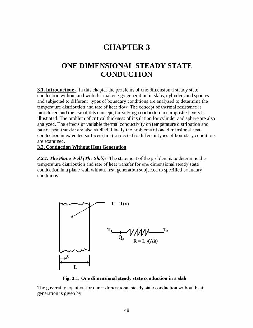
3.1. Introduction:- In this chapter the problems of one-dimensional steady state conduction without and with thermal energy generation in slabs, cylinders and spheres and subjected to different types of boundary conditions are analyzed to determine the temperature distribution and rate of heat flow. The concept of thermal resistance is introduced and the use of this concept, for solving conduction in composite layers is illustrated. The problem of critical thickness of insulation for cylinder and sphere are also analyzed. The effects of variable thermal conductivity on temperature distribution and rate of heat transfer are also studied. Finally the problems of one dimensional heat conduction in extended surfaces (fins) subjected to different types of boundary conditions are examined. 3.2. Conduction Without Heat Generation 3.2.1. The Plane Wall (The Slab):- The statement of the problem is to determine the temperature distribution and rate of heat transfer for one dimensional steady state conduction in a plane wall without heat generation subjected to specified boundary conditions.
The governing equation for one − dimensional steady state conduction without heat generation is given by
x
L
T = T(x)
Fig. 3.1: One dimensional steady state conduction in a slab
Qx
R = L /(Ak)
T2 T1

49
3.2 d2T ----- = 0 ……………………………………(3.1) dx2 Integrating Eq.(3.1) twice with respect to x we get T = C1x + C2 ………………………………(3.2) where C1 and C2 are constants which can be evaluated by knowing the boundary conditions. Plane wall with specified boundary surface temperatures:- If the surface at x = 0 is maintained at a uniform temperature T1 and the surface at x = L is maintained at another uniform temperature T2, then the boundary conditions can be written as follows: (i) at x = 0, T(x) = T1 ; (ii) at x = L, T(x) = T2. Condition (i) in Eq.(3.2) gives T1 = C2. Condition (ii) in Eq. (3.2) gives T2 = C1L + T1 T2 – T1 Or C1 = -------------. L Substituting for C1 and C2 in Eq. (3.2), we get the temperature distribution in the plane wall as x T(x) = (T2 – T1) --- -- + T1 L Or T(x) – T1 x ------------ = -------- ……………………………..(3.3) (T2 – T1) L Expression for Rate of Heat Transfer: The rate of heat transfer at any section x is given by Fourier’s law as Qx = − k A(x) (dT / dx) For a plane wall A(x) = constant = A. From Eq. (3.3), dT/dx = (T2 – T1) / L. Hence Qx = − k A (T2 – T1) / L.

50
3.3
kA(T1 – T2) Or Qx = ---------------- ………………………………..(3.4) L Concept of thermal resistance for heat flow: It can be seen from the above equation that Qx is independent of x and is a constant. Eq.(3.4) can be written as (T1 – T2) (T1 – T2) Qx = -------------- = ------------------ ………………..(3.5) {L /(kA)} R where R = L / (Ak). Eq. (3.5) is analogous to Ohm’s law for flow of electric current. In this equation (T1 – T2) can be thought of as “thermal potential”, R can be thought of as “thermal resistance”,so that the plane wall can be represented by an equivalent “thermal circuit” as shown in Fig.3.1.The units of thermal resistance R are 0 K / W. Plane wall whose boundary surfaces subjected to convective boundary conditions:
Fig.3.2: Thermal Circuit for a plane wall with convective boundary conditions Let T1 be the surface temperature at x = 0 and T2 be the surface temperature at x = L. If we assume that Ti > To, then for steady state conduction heat will transfer by convection from the fluid at Ti to the surface at x = 0, then it is conducted across the plane wall and finally heat is transferred by convection from the surface at x = l to the fluid at To.
x L
Surface in contact with a fluid at To with heat transfer coefficient ho
Surface in contact with a fluid at Ti with heat transfer coefficient hi
Qx Qx Qx Qx To
Ti Rci R Rco
T1 T2

51
3.4 The expression for rate of heat transfer Qx can be written as follows: Qx = hi A [Ti – T1] (Ti – T1) (Ti – T1) or Qx = --------------- = ---------------- ………………………(3.6a) 1 / (hi A) Rci
Rci = 1 / (hiA) is called thermal resistance for convection at the surface at x = 0 (T1 – T2) Similarly Qx = --------------- …………………………………………(3.6b) R where R = L /(Ak) is the thermal resistance offered by the wall for conduction and (T2 – To) Qx = --------------- ………………………………………..(3.6c) Rco Where Rco = 1 / (hoA) is the thermal resistance offered by the fluid at the surface at x = L for convection. It follows from Equations (3.6a), (3.6b) and (3.6c) that (Ti – T1) (T1 – T2) (T2 – T0) Qx = --------------- = ------------------ = -------------- Rci R Rco (Ti – To) Or Qx = ------------------- ……………………………………(3.7) [Rci + R + Rco] 3.2.2. Radial Conduction in a Hollow Cylinder: The governing differential equation for one-dimensional steady state radial conduction in a hollow cylinder of constant thermal conductivity and without thermal energy generation is given by Eq.(2.10b) with n = 1: i.e., d --- [r (dT / dr)] = 0 ………………………….(3.8) dr Integrating the above equation once with respect to ‘r’ we get r (dT / dr) = C1 or (dT / dr) = C1/ r

52
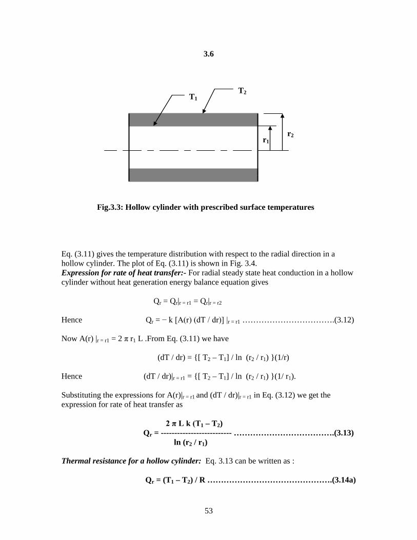
3.5 Integrating once again with respect to ‘r’ we get T(r) = C1 ln r + C2 ………………………..(3.9) where C1 and C2 are constants of integration which can be determined by knowing the boundary conditions of the problem. Hollow cylinder with prescribed surface temperatures: Let the inner surface at r = r1 be maintained at a uniform temperature T1 and the outer surface at r = r2 be maintained at another uniform temperature T2 as shown in Fig. 3.3. Substituting the condition at r1 in Eq.(3.9) we get T1 = C1 ln r1 + C2 ………………………….(3.10a) and the condition at r2 in Eq. (3.9) we get T2 = C1 ln r2 + C2 ………………………….(3.10b) Solving for C1 and C2 from the above two equations we get (T1 – T2) (T1 – T2) C1 = ---------------- = ------------------- [ln r1 – ln r2] ln (r1 / r2) (T1 – T2) and C2 = T1 − ------------------ ln r1 ln (r1 / r2) Substituting these expressions for C1 and C2 in Eq. (3.9) we have (T1 – T2) (T1 – T2) T(r) = -------------- ln r + T1 − ---------------- ln r1 ln (r1 / r2) ln (r1 / r2) or [T(r) – T1] ln (r / r1) --------------- = ------------------- …………………………………………(3.11) [ T2 – T1] ln (r2 / r1)
53
3.6
Eq. (3.11) gives the temperature distribution with respect to the radial direction in a hollow cylinder. The plot of Eq. (3.11) is shown in Fig. 3.4. Expression for rate of heat transfer:- For radial steady state heat conduction in a hollow cylinder without heat generation energy balance equation gives Qr = Qr|r = r1 = Qr|r = r2 Hence Qr = − k [A(r) (dT / dr)] |r = r1 …………………………….(3.12) Now A(r) |r = r1 = 2 π r1 L .From Eq. (3.11) we have (dT / dr) = {[ T2 – T1] / ln (r2 / r1) }(1/r) Hence (dT / dr)|r = r1 = {[ T2 – T1] / ln (r2 / r1) }(1/ r1). Substituting the expressions for A(r)|r = r1 and (dT / dr)|r = r1 in Eq. (3.12) we get the expression for rate of heat transfer as 2 π L k (T1 – T2) Qr = -------------------------- ……………………………….(3.13) ln (r2 / r1) Thermal resistance for a hollow cylinder: Eq. 3.13 can be written as : Qr = (T1 – T2) / R ……………………………………….(3.14a)
r2 r1
T1 T2
Fig.3.3: Hollow cylinder with prescribed surface temperatures

54
3.7
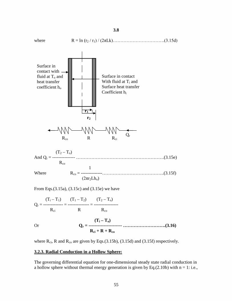
ln (r2 / r1) 1 where R = ----------------- = --------- ……………………………..(3.14b) 2 π L k k Am Where Am = (A2 – A1) / ln (A2 / A1), when A2 = 2π r2 L = Area of the outer surface of the cylinder and A1 = 2π r1 L = Area of the inner surface of the cylinder, and Am is logarithmic mean area. Hollow cylinder with convective boundary conditions at the surfaces:- Let for the hollow cylinder, the surface at r = r1 is in contact with a fluid at temperature Ti with a surface heat transfer coefficient hi and the surface at r = r2 is in contact with another fluid at a temperature To as shown in Fig.3.5.By drawing the thermal circuit for this problem and using the concept of thermal resistance it is easy and straight forward to write down the expression for the rate of heat transfer as shown. (Ti – To) Now Qr = hiAi(Ti
– T1) = 2π r1L hi (Ti – T1) = -------------- ……………..(3.15a) Rci where Rci = 1 / (2π r1Lhi)………………………………………………..(3.15b) (T1 – T2) Also Qr = -------------- …………………………………………………..(3.15c) R
1.0 r2 / r1
r / r1 0
1
(T – T1) (T2 – T1)
Fig. 3.4:Radial temperature distribution for a hollow cylinder
55
3.8 where R = ln (r2 / r1) / (2πLk)…………………………….(3.15d)
(T2 – To) And Qr = --------------- ………………………………………………….(3.15e) Rco
1 Where Rco = --------------…………………………………..(3.15f) (2πr2Lho) From Eqs.(3.15a), (3.15c) and (3.15e) we have (Ti – T1) (T1 – T2) (T2 – To) Qr = ------------- = -------------- = ---------------- Rci R Rco
(Ti – To) Or Qr = ---------------------- ……………………….(3.16) Rci + R + Rco
where Rci, R and Rco are given by Eqs.(3.15b), (3.15d) and (3.15f) respectively. 3.2.3. Radial Conduction in a Hollow Sphere: The governing differential equation for one-dimensional steady state radial conduction in a hollow sphere without thermal energy generation is given by Eq.(2.10b) with n = 1: i.e.,
Surface in contact with fluid at To and heat transfer coefficient ho
Surface in contact With fluid at Ti and Surface heat transfer Coefficient hi
r1
r2
Rco R Rci
Qr
56
3.9 d --- [r2 (dT / dr)] = 0 ………………………….(3.17) dr Integrating the above equation once with respect to ‘r’ we get
r2 (dT / dr) = C1 or (dT / dr) = C1/ r2
Integrating once again with respect to ‘r’ we get T(r) = − C1 / r + C2 ………………………..(3.18) where C1 and C2 are constants of integration which can be determined by knowing the boundary conditions of the problem. Hollow sphere with prescribed surface temperatures: (i) Expression for temperature distribution:-Let the inner surface at r = r1 be maintained at a uniform temperature T1 and the outer surface at r = r2 be maintained at another uniform temperature T2 as shown in Fig. 3.6. The boundary conditions for this problem can be written as follows: (i) at r = r1, T(r) = T1 and (ii) at r = r2, T(r) = T2. Condition (i) in Eq. (3.18) gives T1 = − C1 / r1 + C2 ………………………….(3.19a) Condition (ii) in Eq. (3.18) gives T2 = − C1 / r2 + C2 ………………………….(3.19b) Solving for C1 and C2 from Eqs. (3.19a) and (3.19b) we have (T1 – T2) (T1 – T2) C1 = ------------------- and C2 = T1 + -------------------------- [1 / r2 – 1 / r1] r1[1 / r2 – 1 / r1]
Substituting these expressions for C1 and C2 in Eq. (3.18) we get (T1 – T2) / r (T1 – T2) / r1 T(r) = − ----------------------- + T1 + ---------------------- [1 / r2 – 1 / r1] [1 / r2 – 1 / r1]

57
3.10
Or T(r) – T1 [1 / r2 – 1 / r] ----------------- = ---------------------- ……………………………(3.20) [T1 – T2] [1 / r2 – 1 / r1] (ii) Expression for Rate of Heat Transfer:- The rate of heat transfer for the hollow sphere is given by Qr = −k A(r)(d T / dr) …………………………………………..(3.21) Now at any radius for a sphere A(r) = 4π r2 and from Eq. (3.20) 1 dT / dr = [T1 – T2] ------------------ (1 / r2) [1 / r2 – 1 / r1] Substituting these expressions in Eq. (3.21) and simplifying we get 4 π k r1 r2 [T1 – T2] Qr = -------------------------- ……………………………………...(3.22) [r2 – r1] Eq.(3.22) can be written as Qr = [T1 – T2] / R ……………………………..(3.23a) Where R is the thermal resistance for the hollow sphere and is given by R = (r2 – r1) / {4 π k r1 r2} …………………………………….(3.23b)
r2
r1
Surface at temperature T2
Surface at temperature T1
Fig. 3.6: Radial conduction in a hollow sphere with prescribed surface temperatures

58
3.11 Hollow sphere with convective conditions at the surfaces:- Fig. 3.7 shows a hollow sphere whose boundary surfaces at radii r1 and r2 are in contact with fluids at temperatures Ti and T0 with surface heat transfer coefficients hi and h0 respectively.
The thermal resistance network for the above problem is shown in Fig.3.8
.Fig. 3.8: Thermal circuit for a hollow sphere with convective boundary conditions
r2
r1
Surface in contact with fluid at T0 and surface heat transfer coefficient h0
Surface in contact with fluid at Ti and surface heat transfer coefficient hi
Fig. 3.7: Radial conduction in a hollow sphere with convective conditions at the two boundary surfaces
Rci R Rco
Qci = Qr = Qco ………………(3.24)
Where Qci = heat transfer by convection from the fluid at Ti to the inner surface of the hollow sphere and is given by [Ti – T1]
Qci = hi Ai [Ti – T1] = --------------- …..(3.25) Rci
Qr
Qco
To Ti Qci

59
3.12 When T1 = the inside surface temperature of the sphere and Rci = 1 / (hiAi) = the thermal resistance for convection for the inside surface Or Rci = 1 / (4 π r1
2 hi) ……………………………………………………….(3.25b) Qr = Rate of heat transfer by conduction through the hollow sphere = [T1 – T2] / R with R = (r2 – r1) / {4 π k r1 r2} And Qco = Rate of heat transfer by convection from the outer surface of the sphere to the outer fluid and is given by [T2 – T0]
Qco = ho Ao [T2 – To] = --------------- ……………(3.26a) Rco Where T2 = outside surface temperature of the sphere and Ao = outside surface area of the sphere = 4 π r2
2 so that Rco = 1 / {4 π r2
2 ho}…………………………….(3.26b) Now Eq.(3.24) can be written as [Ti – T1] [T1 – T2] [T2 – T1] Qr = hi Ai [Ti – T1] = -------------- = ---------------- = ---------------- Rci R Rco [Ti – To] Qr = ---------------------- …………………………………………(3.27) [Rci + R + Rco] 3.2.4. Steady State conduction in composite medium: There are many engineering applications in which heat transfer takes place through a medium composed of several different layers, each having different thermal conductivity. These layers may be arranged in series or in parallel or they may be arranged with combined series-parallel arrangements. Such problems can be conveniently solved using electrical analogy as illustrated in the following sections. Composite Plane wall:- (i) Layers in series: Consider a plane wall consisting of three layers in series with perfect thermal contact as shown in Fig. 3.10.The equivalent thermal

60
3.13 resistance network is also shown. If Q is the rate of heat transfer through an area A of the composite wall then we can write the expression for Q as follows:
Fig. 3.10: A composite plane wall with three layers in series and the equivalent thermal resistance network (T2 – T3) (T1 – T2) (T1 – T2) (T2 – T3) (T3 – Tco) Q = -------------- = --------------- = ------------- = ------------ = ---------------- Rco R1 R2 R3 Rco (Ti – T0) Ti – T0) Or Q = --------------------------------- = ------------…………………………….(3.28) Rci + R1 + R2 + R3 + Rco Rtotal
Overall heat transfer coefficient for a composite wall:- It is sometimes convenient to express the rate of heat transfer through a medium in a manner which is analogous to the Newton’s law of cooling as follows: If U is the overall heat transfer coefficient for the composite wall shown in Fig. (3.10) then Q = U A (Ti – To) ………………………………...(3.29) Comparing Eq. (3.28) with Eq. (3.29) we have the expression for U as 1 U = --------------- ……………………………………..(3.30) A Rtotal
Surface in contact with fluid at Ti and surface heat transfer coefficient hi
Surface in contact with a fluid at T0 and surface heat transfer coefficient ho
L2 L1 L3
k1 k2 k3
T1 T2 T3 T4
Q Q
Rci R1 R2 R3 Rco
Ti T1 T2 T3 T4 To

61
3.14 1 1 Or U = ------------------------------------= ----------------------------------------------------- A [ Rci + R1 + R2 + R3 ] A[1/(hiA) + L1/(Ak1) + L2/(Ak2) + L3/(Ak3)] 1 Or U = --------------------------------------------……………………………………(3.31) [ 1/hi + L1 / k1 + L2 / k2 + L3 / k3 ] (ii) Layers in Parallel:- Fig.3.11 shows a composite plane wall in which three layers are
FFig. 3.11: Schematic and equivalent thermal circuit for a composite wall with layers in parallel arranged in parallel. Let ‘b’ be the dimension of these layers measured normal to the plane of the paper. Let one surface of the composite wall be in contact with a fluid at temperature Ti and surface heat transfer coefficient hi and the other surface of the wall be in contact with another fluid at temperature To with surface heat transfer coefficient ho. The equivalent thermal circuit for the composite wall is also shown in Fig. 3.11. The rate of heat transfer through the composite wall is given by Q = Q1 + Q2 + Q3 ………………………….(3.32)
L
b
H1 H2 H3
k1 k2 k3
Surface in contact with fluid at Ti with heat transfer coefficient hi
Ti
Rci
R1
R2
R3
Rco To
Q1
Q2
Q3
T1 T2
Q
Suface in contact with fluid at To and surface heat transfer coefficient ho
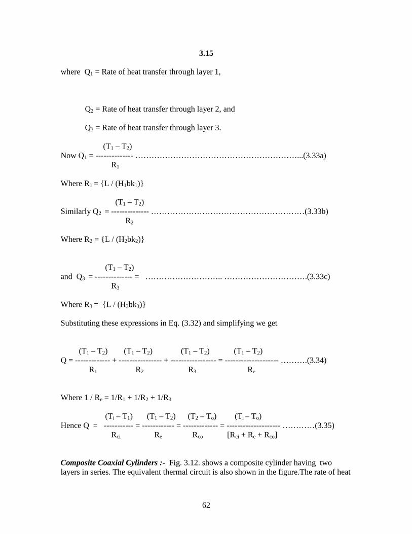
62
3.15 where Q1 = Rate of heat transfer through layer 1,
Q2 = Rate of heat transfer through layer 2, and Q3 = Rate of heat transfer through layer 3. F (T1 – T2) Now Q1 = -------------- ……………………………………………………...(3.33a) R1 Where R1 = {L / (H1bk1)} F (T1 – T2) Similarly Q2 = -------------- …………………………………………………(3.33b) R2 Where R2 = {L / (H2bk2)} and (T1 – T2) and Q3 = -------------- = ……………………….. ………………………….(3.33c) R3 Where R3 = {L / (H3bk3)} Substituting these expressions in Eq. (3.32) and simplifying we get
(T1 – T2) (T1 – T2) (T1 – T2) (T1 – T2) Q = ------------- + ---------------- + ----------------- = -------------------- ……….(3.34) R1 R2 R3 Re
Where 1 / Re = 1/R1 + 1/R2 + 1/R3
(Ti – T1) (T1 – T2) (T2 – To) (Ti – To) Hence Q = ----------- = ------------ = ------------- = -------------------- …………(3.35) Rci Re Rco [Rci + Re + Rco] Composite Coaxial Cylinders :- Fig. 3.12. shows a composite cylinder having two layers in series. The equivalent thermal circuit is also shown in the figure.The rate of heat

63
3.16 transfer through the composite layer is given by
(Ti – T1) (T1 – T2) (T2 – T3) (T3 – To) (Ti – T0) Now Q = ------------- = ------------ = ----------- = ------------- = ----------------------------- Rci R1 R2 Rco [Rci + R1 + R2 + Rco] ……………..(3.36) 1 1 Where Rci = 1 / [hiAi] = -------------- ; R1 = ---------- ln (r2 / r1) 2 π r1L hi 2 π L k1 1 1 Rco = 1 / [hoAo] = -------------- ; R2 = ---------- ln (r3 / r2) 2 π r3L ho 2 π L k2 The above expression for Q can be extended to any number of layers.
r1
r2 r3
Surface in contact with fluid at To and surface heat transfer coefficient h0
Surface in contact with fluid at Ti and surface heat transfer coefficient hi
k1
k2
Q Rci R1 R2 Rco
Ti T1 T2 T3 To
Fig. 3.12: Schematic and thermal circuit diagrams for a composite cylinder

64
3.17
Overall Heat Transfer Coefficient for a Composite Cylinder:- For a cylinder the area of heat flow in radial direction depends on the radius r we can define the overall heat transfer coefficient either based on inside surface area or based on outside surface area of the composite cylinder. Thus if Ui is the overall heat transfer coefficient based on inside surface area Ai and Uo is the overall heat transfer coefficient based on outside surface area Ao then Q = UiAi (Ti
– To) ………………………………………………………………….(3.37) From equations (3.36) and (3.37) we have (Ti – T0) Now UiAi (Ti
– To) = ----------------------------- [Rci + R1 + R2 + Rco] Substituting the expressions for Ai, Rci,R1,R2 and Rco in the above equation we have 1 2 π r1L Ui = -------------------------------------------------------------------------------------------- [1 /(2πr1Lhi) + {1/(2πLk1)}ln (r2 / r1) + {1/(2πLk2)}ln (r3 / r2) + 1/(2πr3Lho)] 1 Or Ui = ------------------------------------------------------------------------- ……..(3.38) [ 1/hi + (r1 / k1) ln (r2/r1) + (r1/k2) ln (r3/r2) + (r1/r3) (1/ho) ] Similarly it can be shown that 1 Uo = ------------------------------------------------------------------------------ …..(3.39) [(r3/ r2) (1/hi ) + (r3 / k1) ln (r2/r1) + (r3/k2) ln (r3/r2) + (1/ho) ] Composite Concentric Spheres:- Fig.3.13 shows a composite sphere having two layers with the inner surface of the composite sphere in contact with fluid at a uniform temperature Ti and surface heat transfer coefficient hi and the outer surface in contact with another fluid at a uniform temperature To and surface heat transfer coefficient ho. The corresponding thermal circuit diagram is also shown in the figure.

65
3.18
Eq. (3.36) is also applicable for the composite sphere of Fig. 3.13 except that the expression for individual resistance will be different. Thus (Ti – To) Q = --------------------------- …………………………………………….(3.40) [Rci + R1 + R2 + Rco] 1 1 (r2 – r1) where Rci = ---------- = ----------------- ; R1 = --------------- ; hi Ai 4 π r1
2 hi 4 π k1 r1r2 1 1 (r3 – r2) Rco = ---------- = ----------------- ; R2 = --------------- ; hoAo 4 π r3
2 ho 4 π k2 r2r3
r1
Surface in contact with fluid at Ti and surface heat transfer coefficient hi
k1
k2
Q Rci R1 R2 Rco
Ti T1 T2 T3 To
Fig. 3.13: Schematic and thermal circuit diagrams for a composite sphere
Surface in contact with fluid at To and surface heat transfer coefficient h0
r1 r2 r3

66
3.19
Example 3.1:- Consider a plane wall 100 mm thick and of thermal conductivity 100
W/(m-K). Steady state conditions are known to exist with T1 = 400 K and T2 = 600 K. Determine the heat flux (magnitude and direction) and the temperature gradient dT/dx for the coordinate system shown in Fig. P3.1.(2000 0C/m; - 200,00 W/m2;- 2000 0C/m,200,000 W/m2; 2000 0C/m, - 200,000 W/m2)
Solution:-
T(x) T(x) T(x)
x x x
T2
T1 T1
T2 T2
T1
Fig. P3.1 : Schematic for problem 3.1
L L L
(a) (b) (c)

67
3.20
(b)
x
T(x)
T2 T1 L
It can be seen from the figure shown that temperature is decreasing with increase in x or in other words dT/dx is – ve. Therefore dT/dx = (T1 – T2)/L = (400 – 600) / 0.1 = ─ 2000 0 C / m. qx = ─ k dT/dx = ─ 100 x (─ 2000) = + 200,000 W / m2. + ve sign for qx indicates that heat transfer is taking place in the + ve direction of x.
T(x), k=100 w/m-k
x
L
T1 T2
(a) It can be seen from the figure that the temperature is increasing with increase in x: i.e., dT/dx is +ve. Therefore dT/dx = (T2 – T1) / L = (600 – 400)/0.10 = 2000 0C / m. Heat flux = qx = ─ k dT/dx = ─ 100 x 2000 W/m2 = ─ 2 x 10 5 W / m2. The negative sign indicates that heat transfer takes place in the direction opposite to the +ve direction of x.
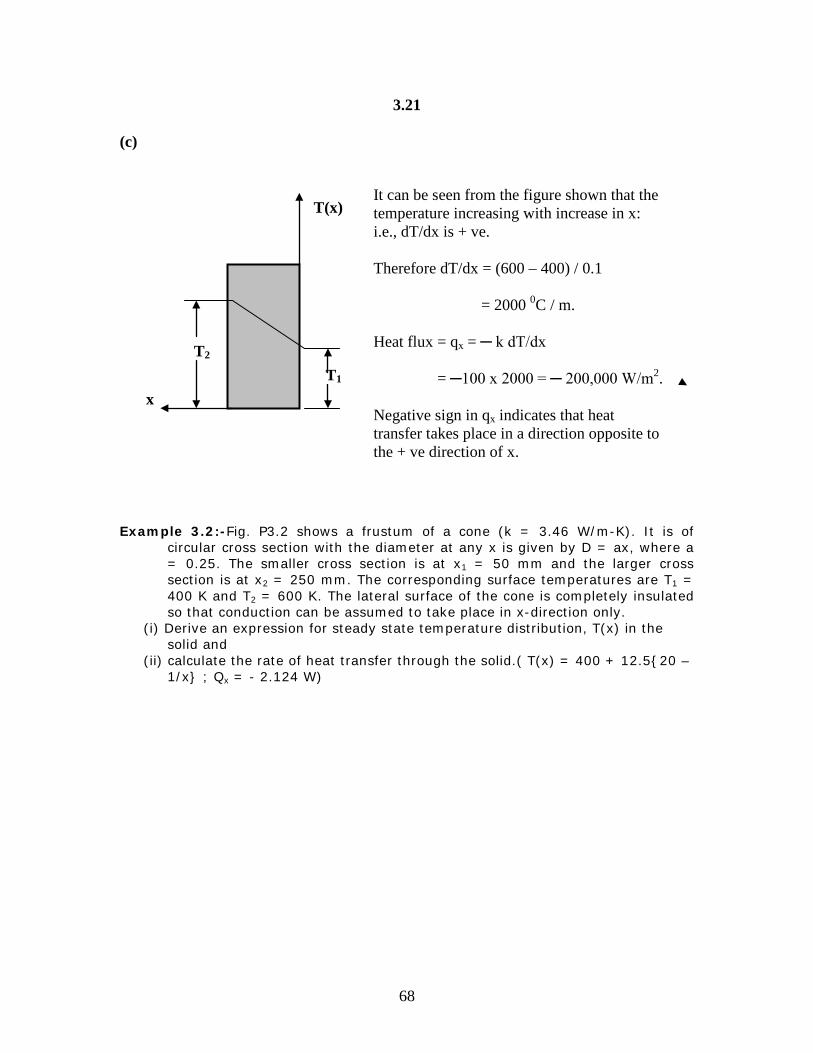
68
3.21 (c)
Example 3.2:-Fig. P3.2 shows a frustum of a cone (k = 3.46 W/m-K). It is of circular cross section with the diameter at any x is given by D = ax, where a = 0.25. The smaller cross section is at x1 = 50 mm and the larger cross section is at x2 = 250 mm. The corresponding surface temperatures are T1 = 400 K and T2 = 600 K. The lateral surface of the cone is completely insulated so that conduction can be assumed to take place in x-direction only.
(i) Derive an expression for steady state temperature distribution, T(x) in the solid and
(ii) calculate the rate of heat transfer through the solid.( T(x) = 400 + 12.5{20 – 1/x} ; Qx = - 2.124 W)
T2
T1
T(x)
x
It can be seen from the figure shown that the temperature increasing with increase in x: i.e., dT/dx is + ve. Therefore dT/dx = (600 – 400) / 0.1 = 2000 0C / m. Heat flux = qx = ─ k dT/dx = ─100 x 2000 = ─ 200,000 W/m2. Negative sign in qx indicates that heat transfer takes place in a direction opposite to the + ve direction of x.
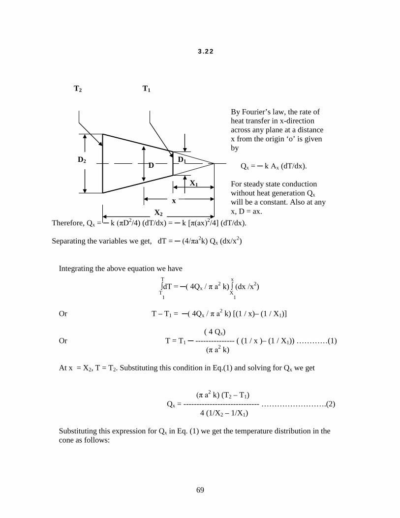
69
3.22
Integrating the above equation we have T x ∫dT = ─( 4Qx / π a2 k) ∫ (dx /x2) T1 X1 Or T – T1 = ─( 4Qx / π a2 k) [(1 / x)– (1 / X1)] ( 4 Qx) Or T = T1 ─ --------------- ( (1 / x )– (1 / X1)) …………(1) (π a2 k) At x = X2, T = T2. Substituting this condition in Eq.(1) and solving for Qx we get (π a2 k) (T2 – T1) Qx = ----------------------------- …………………….(2) 4 (1/X2 – 1/X1) Substituting this expression for Qx in Eq. (1) we get the temperature distribution in the cone as follows:
X1
x X2
D2 D1 D
By Fourier’s law, the rate of heat transfer in x-direction across any plane at a distance x from the origin ‘o’ is given by Qx = ─ k Ax (dT/dx). For steady state conduction without heat generation Qx will be a constant. Also at any x, D = ax.
T2 T1
Therefore, Qx = ─ k (πD2/4) (dT/dx) = ─ k [π(ax)2/4] (dT/dx). Separating the variables we get, dT = ─ (4/πa2k) Qx (dx/x2)

70
3.23 (T2 – T1) (1/x – 1/X1) T(x) = T1 + --------------------------------- ………………..(3) (1/X2 – 1/X1) Substituting the given numerical values for X1, X2, T1 and T2 in Eq.(3) we get the temperature distribution as follows: (600 – 400) [ 1/ x – 1/0.05] T(x) = 400 + ------------------------------------ [ 1/0.25 – 1/0.05} Or T(x) = 400 + 12.5 [ 20 – 1/x] Temperature distribution π x (0.25)2 x 3.46 x [ 600 – 400 ] And Qx = -------------------------------------------- = ─ 2.123 W 4 x [ 1/0.25 – 1/0.05 ] Example 3.3:-A plane composite wall consists of three different layers in perfect
thermal contact. The first layer is 5 cm thick with k = 20 W/(m-K), the second layer is 10 cm thick with k = 50 W/(m-K) and the third layer is 15 cm thick with k = 100 W/(m-K). The outer surface of the first layer is in contact with a fluid at 400 0C with a surface heat transfer coefficient of 25 W/(m2 – K), while the outer surface of the third layer is exposed to an ambient at 30 0C with a surface heat transfer coefficient of 15 W/(m2-K).Draw the equivalent thermal circuit indicating the numerical values of all the thermal resistances and calculate the heat flux through the composite wall. Also calculate the overall heat transfer coefficient for the composite wall.
Solution: Data :- L1 = 0.05 m ; L2 = 0.10 m ; L3 = 0.15 m ; k1 = 20 W /(m-K) ; k2 = 50 W /(m-K) ; k3 = 100 W/(m-K) ; hi = 25 W /(m2 – K) ; h0 = 15 W/(m2 – K) ;
Ti = 400 0 C ; T0 = 30 0 C. 1 Rci = 1 / (hiA1) = ---------------- = 0.04 m2 – K / W (A1 = A2 = A3 = A4 = 1 m2) 25 x 1
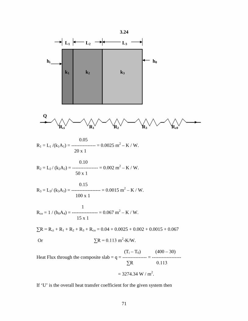
71
3.24
0.05 R1 = L1 /(k1A1) = --------------- = 0.0025 m2 – K / W. 20 x 1 0.10 R2 = L2 / (k2A2) = ---------------- = 0.002 m2 – K / W. 50 x 1 0.15 R3 = L3/ (k3A3) = ------------------ = 0.0015 m2 – K / W. 100 x 1 1 Rco = 1 / (h0A4) = ---------------- = 0.067 m2 – K / W. 15 x 1 ∑R = Rci + R1 + R2 + R3 + Rco = 0.04 + 0.0025 + 0.002 + 0.0015 + 0.067
Or ∑R = 0.113 m2-K/W. (Ti – T0) (400 – 30) Heat Flux through the composite slab = q = --------------- = ------------------ ∑R 0.113 = 3274.34 W / m2. If ‘U’ is the overall heat transfer coefficient for the given system then
L3 L2 L1
k1 k2 k3
hi h0
Rci R1 R2 R3 Rc0
Q

72
3.25
Q 1 1 U = ---------------- = ------------- = -------------- (Ti – T0) ∑R 0.113 = 8.85 W / (m2 – K). Example 3.4:-A composite wall consisting of four different materials is shown in Fig
P3.10. Using the thermal resistance concept determine the heat transfer rate per m2 of the exposed surface for a temperature difference of 300 0 C between the two outer surfaces. Also draw the thermal circuit for the composite wall.
Solution: 0.04 R1 = L1 / (A1k1) = ---------------- = 0.0002 0 C / W. 2 x 100 0.10 R2 = L2 / (A2k2) = ---------------- = 0.00143 0 C / W. 1 x 70 0.10 R3 = L3 / (A3k3) = --------------- = 0.005 0 C / W. 1 x 20
10 cm 4cm 5 cm
1 m
2 m
k1 k2 k4
k3
k1 = 100 W/(m-K) ; L1 =0.04 m; k2 = 0.04 W/(m-K) ; L2 = 0.1 m; k3 = 20 W/(m-K) ; L3 = 0.1 m ; k4 = 70 W/(m-K) ; L4 = 0.05 m; W = Width of the wall perpendicular to the plane of paper = 1 m (assumed). T1 – T4 = 300 0 C. A1 = A4 = 1 x 2 = 2 m2. A2 = A3 = 1 x 1 = 1 m2.
T1
k2
k3

73
3.26 0.05 R4 = L4 / (A4k4) = ------------------ = 0.00036 0 C / W. 2 x 70
(T1
– T4) 300 Q = --------------------- = ------------------------------------ = 86.705 x 10³ W (R1 + Re + R4) [0.002 + 0.0011 + 0.00036] Heat transfer per unit area of the exposed surface is given by q = Q / A1 = 86.705 / 2.0 = 43.35 kW. Example 3.5:-A composite cylindrical wall is composed of two materials of thermal
conductivity kA and kB. A thin electric resistance heater for which the interfacial contact resistances are negligible separates the two materials. Liquid pumped through the inner tube is at temperature Ti with the inside surface heat transfer coefficient hi. The outer surface of the Composite wall is
exposed to an ambient at a uniform temperature of To with the outside surface heat transfer coefficient ho. Under steady state conditions a uniform heat flux of qh is dissipated by the heater.
(a) Sketch the equivalent thermal circuit for the composite wall and express all thermal resistances in terms of the relevant variables
(b)Obtain an expression that may be used to determine the temperature of the heater,Th.
(b) Obtain an expression for the ratio of heat flows to the outer and inner fluid, qo/qi.
R1
R3
R4
Thermal potential = T1 – T4
R2 and R3 are resistances in parallel and they can be replaced by a single equivalent resistance Re, where R2 R3 0.00143 x 0.005 1 / Re = 1 / R2 + 1 / R3 or Re = --------------- = ----------------------- = 0.0011 0C/W (R2 + R3) (0.00143 + 0.005) Now R1, Re and R4 are resistances in series so that
R2 Q

74
3.27 Solution:
1 1 1 Ri = ------------- ln (r1/ri) ; Rci = ------------------ = --------------------- (2π LkA) hi Ai (2π ri L hi) 1 1 1 Ro = ------------- ln (ro/r1) ; Rco = ------------------ = --------------------- (2π LkB) ho Ao (2π ro L ho) Qi = (Th – Ti) / [Ri + Rci ] ; Qo = (Th – To) / [Ro + Rco] ; Qtotal = Qi + Qo = (Th – Ti) / (Ri + Rci) + (Th – To)/ (Ro + Rco) (Th – Ti) (Th – To) 2π r1L q h = -------------------------- + ----------------------- ln (r1/ri) 1 ln (ro/r1) 1 ---------- + ------------- ---------- + ------------- 2π L kA 2π L ri hi 2π L kB 2π L ro ho
ri r1
ro
heater
Qi
Q0
hi,Ti
ho,To
kA
kB
Qi
Qo
Qtotal
Ri Rci
Ro Rco
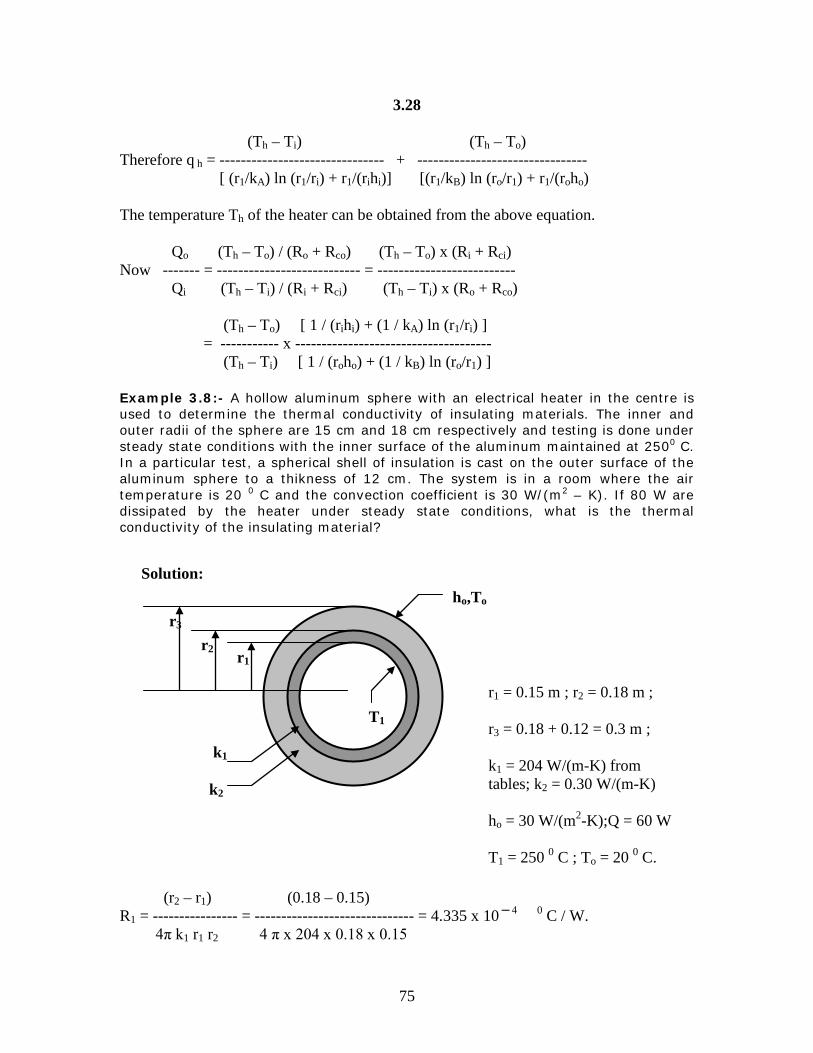
75
3.28 (Th – Ti) (Th – To) Therefore q h = ------------------------------- + -------------------------------- [ (r1/kA) ln (r1/ri) + r1/(rihi)] [(r1/kB) ln (ro/r1) + r1/(roho) The temperature Th of the heater can be obtained from the above equation.
Qo (Th – To) / (Ro + Rco) (Th – To) x (Ri + Rci) Now ------- = --------------------------- = -------------------------- Qi (Th – Ti) / (Ri + Rci) (Th – Ti) x (Ro + Rco) (Th – To) [ 1 / (rihi) + (1 / kA) ln (r1/ri) ] = ----------- x ------------------------------------- (Th – Ti) [ 1 / (roho) + (1 / kB) ln (ro/r1) ] Example 3.8:- A hollow aluminum sphere with an electrical heater in the centre is used to determine the thermal conductivity of insulating materials. The inner and outer radii of the sphere are 15 cm and 18 cm respectively and testing is done under steady state conditions with the inner surface of the aluminum maintained at 2500 C. In a particular test, a spherical shell of insulation is cast on the outer surface of the aluminum sphere to a thikness of 12 cm. The system is in a room where the air temperature is 20 0 C and the convection coefficient is 30 W/(m2 – K). If 80 W are dissipated by the heater under steady state conditions, what is the thermal conductivity of the insulating material?
(r2 – r1) (0.18 – 0.15) R1 = ---------------- = ------------------------------ = 4.335 x 10 ─ 4 0 C / W. 4π k1 r1 r2 4 π x 204 x 0.18 x 0.15
r1 r2
r3
k1 k2
T1
ho,To
r1 = 0.15 m ; r2 = 0.18 m ; r3 = 0.18 + 0.12 = 0.3 m ; k1 = 204 W/(m-K) from tables; k2 = 0.30 W/(m-K) ho = 30 W/(m2-K);Q = 60 W T1 = 250 0 C ; To = 20 0 C.
Solution:

76
3.29 (r3 – r2) (0.30 – 0.18) R2 = ---------------- = ------------------------------ = 0.177 / k2 0 C / W. 4π k2 r2 r3 4 π x k2 x 0.30 x 0.18 1 1 Rco = 1 / (hoAo) = ------------------- = --------------------- = 0.0295 0 C / W. 4π r3
2 ho 4π x (0.3)2 x 30 (T1 – To) Q = -------------------- or R2 = (T1 – To) / Q – (R1 + Rco) R1 + R2 + Rco Or R2 = (250 – 20) / 80 ─ (4.335 x 10 ─ 4 + 0.0295) = 2.874 Therefore 0.177 / k2 = 2.845 Or k2 = 0.177 / 2.845 = 0.062 W / (m-K) Example 3.8:- In a hollow sphere of inner radius 10 cm and outer radius 20, the inner surface is subjected to a uniform heat flux of 1.6 x 10 5 W/m2 and the outer surface is maintained at a uniform temperature of 0 0C.The thermal conductivity of the material of the sphere is 40 W /(m – K).Assuming one-dimensional radial steady state conduction determine the temperature of the inner surface of the hollow sphere. Solution:-
The governing equation for one-dimensional steady-state radial conduction in a sphere without heat generation is given by d/dr ( r2 dT / dr ) = 0 …………………………………..(1)
R1
R2
q0
T0

77
3.30 The boundary conditions are : (i) at r = R1, ─ k (dT/dr)|r=R1 = q0 (ii) at r = R2 T(r) = 0. Integrating Eq. (1) w.r.t. r once, we get r2 (dT/dr) = C1 or dT / dr = C1 / r2 …………………………(2) Integrating once again w.r.t. r we get T(r) = ─ C1 / r + C2 ……………….. (3) From (2) (dT/dr)r = R1 = C1 / R1
2
Hence condition (i) gives ─ kC1 / R1
2 = q0 Or C1 = ─ q0 R1
2 / k
Condition (ii) in Eq.(2) gives 0 = ─ C1 / R2 + C2 Or C2 = C1 / R2 = ─ (q0R1
2) / (kR2) Substituting the expressions for C1 and C2 in Eq. (2) we have q0 R1
2 q0 R12
T(r) = -------------- ─ ------------------- k r k R2 Substituting the numerical values for q0, k, R1 and R2 we have 1.6 x 105 x 0.12 1.6 x 105 x 0.12 T(r) = -------------------- / r ─ --------------------
40 40 x 0.2 Or T(r) = (40 / r) ─ 200

78
3.31 Therefore T(r) |r = R1 = (40 / 0.1) ─ 200 = 200 0 C. 3.2.5. Thermal Contact Resistance: In the analysis of heat transfer problems for composite medium it was assumed that there is “perfect thermal contact” at the interface of two layers. This assumption is valid only the two surfaces are smooth and they produce a perfect contact at each point.But in reality, even flat surfaces that appear smooth to the naked eye would be rather rough when examined under a microscope as shown in Fig. 3.14 with numerous peaks and valleys.
The physical significance of thermal contact resistance is that the peaks will form good thermal contact, but the valleys will form voids filled with air.As a result the air gaps act as insulation because of poor thermal conductivity of air.Thus the interface offers some resistance to heat conduction and this resistance is called the “thermal contact resistance,Rcont”. The value of Rcont is determined experimentally and is taken into account while analyzing the heat conduction problems involving multi-layer medium.The procedure is illustrated by means of a few examples below. Example 3.4:- A composite wall consists of two different materials A [k = 0.1 W/(m-k)] of thickness 2 cm and B[ k = 0.05 W/(m-K)] of the thickness 4 cm. The outer surface of layer A is in contact with a fluid at 2000C with a surface heat transfer coefficient of 15 W/(m2-K) and the outer surface of layer B is in contact with another fluid at 50 0 C with a surface heat transfer coefficient of 25 W/(m2-K). The contact resistance between layer A and layer B is 0.33 (m2-K) /W. Determine the heat transfer rate through the composite wall per unit area of the surface. Also calculate the interfacial temperatures and the inner and outer surface temperatures.
T1 Tc1
Tc2 T2
Gap between solids
T2 T1
LB LA
Rcont
Fig.3.14: Temperature drop across a contact resistance
Enlarged view of the contact surface
.

79
3.32 Solution:
R2 = LB / (kBAB) = 0.04 / (0.05 x 1) = 0.8 m2 – K / W. Rco = 1 / (hoAB) = 1 / ( 25 x 1) = 0.04 m2 – K / W. ∑R = Rci + R1 + Rcont + R2 + Rco = 0.067 + 0.2 + 0.33 + 0.8 + 0.04 = 1.437 m2 – K / W. (200 – 50) Heat flux = q = (Ti – To) / ∑R = ------------------ = 104.4 W/m2 1.437 Now q = (Ti – TA) / Rci or TA = Ti – q Rci = 200 – (104.4 x 0.067) = 193 0 C. Similarly Tc1 = TA – q R1 = 193 – (104.4 x 0.2) = 172.12 0 C. Tc2 = Tc1 – q Rcont = 172.12 – (104.4 x 0.33) = 137.67 0 C. TB = Tc2 – q R2 = 137.67 – (104.4 x 0.8) = 54.15 0 C. Check : To = TB – q Rco = 54.15 – (104.4 x 0.04) = 49.97 0 C
T1 Tc1
Tc2 T2
kA kB
h0,T0 hi,Ti Ti = 200 0 C ; T0 = 50 0 C ; hi = 15 W/(m2 – K) ; h0 = 25W/(m2– K) kA = 0.1 W/(m-K) ; kB = 0.05 W/(m-K) Rcont = 0.33 (m2 – K) /W. The equivalent thermal circuit is also shown in the figure. 1 Rci = 1/(hiAA) = ------- = 0.067 m2-K/W (15 x 1) R1 = LA/(kAAA) = 0.02 / (0.1 x 1) = 0.2 m2-K / W.
LB LA
Rcont

80
3.33 Example 3.6:- A very thin electric heater is wrapped around the outer surface of a
long cylindrical tube whose inner surface is maintained at 5 0C. The tube wall has inner and outer radii of 25 mm and 75 mm respectively and a thermal conductivity of 10 W/(m-K). The thermal contact resistance between the heater and the outer surface of the tube per unit length is 0.01 (m-K) / W. The outer surface of the heater is exposed to a fluid with a temperature of – 10 0C and a convection coefficient of 100 W/(m2-K). Determine the heater power required per length of the tube to maintain a heater temperature of 25 0C.
Solution: Data: r1 = 0.025 m ; r2 = 0.075 m ; k = 10 W /(m-K) ; T∞ = ─ 10 0 C ; h = 100 W/(m2 – K); T1 = 5 0 C ; Rcont = 0.01 m – K / W ; T2 = 25 0 C.
Fig. P3.6: Schematic and Thermal circuit for Example 3.6 1 Rco = 1 / (h Ao) = ----------------------- = 0.0212 (m- K) / W. 100 x 2π x 0.075 1 1 Rcond = ------------- ln (r2 / r1) = ------------------ ln (0.075 / 0.025) = 0.0175 (m-K) / W. 2π L k (2x π x 1 x 10)
r2 r1
T1
Heater h,T∞
Qamb
Qtube
Qtotal
Qamb
Qtube
Rco
Rcont Rcond
T2
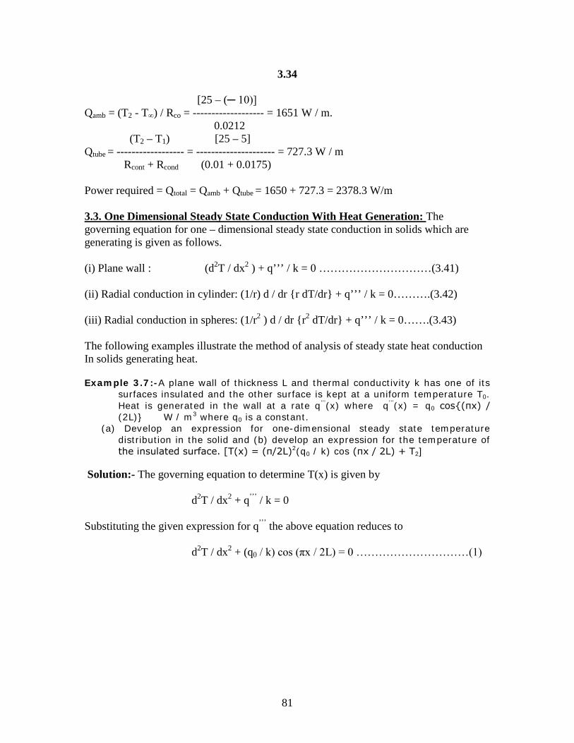
81
3.34 [25 – (─ 10)] Qamb = (T2 - T∞) / Rco = ------------------- = 1651 W / m. 0.0212 (T2 – T1) [25 – 5] Qtube = ------------------ = --------------------- = 727.3 W / m Rcont + Rcond (0.01 + 0.0175) Power required = Qtotal = Qamb + Qtube = 1650 + 727.3 = 2378.3 W/m 3.3. One Dimensional Steady State Conduction With Heat Generation: The governing equation for one – dimensional steady state conduction in solids which are generating is given as follows.
(i) Plane wall : (d2T / dx2 ) + q’’’ / k = 0 …………………………(3.41) (ii) Radial conduction in cylinder: (1/r) d / dr {r dT/dr} + q’’’ / k = 0……….(3.42) (iii) Radial conduction in spheres: (1/r2 ) d / dr {r2 dT/dr} + q’’’ / k = 0…….(3.43) The following examples illustrate the method of analysis of steady state heat conduction In solids generating heat. Example 3.7:-A plane wall of thickness L and thermal conductivity k has one of its
surfaces insulated and the other surface is kept at a uniform temperature T0. Heat is generated in the wall at a rate q’’’(x) where q’’’(x) = q0 cos{(πx) / (2L)} W / m3 where q0 is a constant.
(a) Develop an expression for one-dimensional steady state temperature distribution in the solid and (b) develop an expression for the temperature of the insulated surface. [T(x) = (π/2L)2(q0 / k) cos (πx / 2L) + T2]
Solution:- The governing equation to determine T(x) is given by d2T / dx2 + q’’’ / k = 0 Substituting the given expression for q’’’ the above equation reduces to d2T / dx2 + (q0 / k) cos (πx / 2L) = 0 …………………………(1)

82
3.35
The boundary conditions are ; (i) at x = 0 (dT/dx) = 0 (Insulated) (ii) at x = L, T = T1
Integrating Eq.(1) once w.r.t. x we get dT/dx = -(π/2L) (q0/k) sin (πx/2L) + C1 ……………(2) Integrating once again w.r.t. x we get T(x) = -(π/2L)2 (q0/k) cos (πx/2L) + C1x + C2 …………….(3) Condition (i) in Eq. (2) gives 0 = 0 + C1 or C1 = 0. Condition (ii) in Eq. (3) gives T1 = 0 + 0 + C2 or C2 = T1. Substituting the values of C1 and C2 in Eq. (3) we get the temperature distribution as T(x) = -(π/2L)2 (q0/k) cos (πx/2L) + T1 …………………..(4). At the insulated surface (x = 0) the temperature therefore is given by T(x) |x=0 = (π/2L)2 (q0/k) + T1. Example 3.8:- A long cylindrical rod of radius 5 cm and k = 10 W/(m-K) contains
radioactive material which generates heat uniformly within the cylinder at a rate of 3x10 5 W/ m3. The rod is cooled by convection from its cylindrical
L Insulated T 1
x
T = T(x) q’’’= q0 cos (πx/2L)

83
3.36 surface by ambient air at 50 0C with a heat transfer coefficient of 60 W/(m2-K).
Assuming one-dimensional radial conduction determine the temperature at the centre of the rod as well as at the outer surface of the rod.(175 0 C)
Eq. (1) can be written as d / dr (r dT/dr) + q’’’ r / k = 0. Integrating once w.r.t. r we get r dT/dr + (q’’’ r2) / 2k = C1
or dT/dr + (q’’’ r) / 2k = C1 / r ………………… (2) Integrating once again w.r.t. r we have q’’’ r2
T(r) = ─ -------------- + C1 ln r + C2 …………(3) 4 k Condition (i) in Eq. (2) gives 0 + 0 = C1 / 0 or C1 = 0. From Eq. (3) we have q’’’ R2
T(r)|r=R = ─ -------------- + C2 …………………..(3) 4 k and from Eq. (2) we have (dT/dr) |r=R = ─(q’’’ R) / 2k Therefore condition (ii) gives
R
q’’’
T = T(r)
The governing differential equation to determine one-dimensional steady state radial conduction with heat generation is given by (1/r) d / dr (r dT/dr) + q’’’ / k = 0………………………..(1) The boundary conditions are : (i) at r = 0, dT/dr = 0 (axis of symmetry) (ii0 at r= R, ─ k (dT/dr)|r=R = h [T |r= ─ T∞]
h, T∞
84
3.37 ─ k [─ (q’’’/R) / 2k] = h [ ─ (q’’’ R2 /4k) + C2 ─ T∞] q’’’ R q’’’ R2
Or C2 = ----------- + -------------- + T∞ 2 h 4 k Substituting the expressions for C1 and C2 in Eq.(3) we get the temperature distribution in the cylinder as q’’’ R2
T(r) = T∞ + ------------- [ 1 –(r/R)2 ] + (q’’’R) / 2h …………………(4) 4 k 3 x 10 5 x (0.05)2
Now q’’’R2 / (4 k) = ----------------------- = 18.75 0 C. 4 x 10 3 x 10 5 x 0.05 q’’’R / (2h) = ------------------------ = 125 0 C 2 x 60 Therefore T(r) = 50 + 18.75 [ 1 – (r/R)2] + 125 = 175 + 18.75 [ 1 – (r/R)2] At the centre T(r) |r=0 = 175 + 18.75 = 193.75 0 C. At the surface T(r) |r=R = 5 0+ 18.75 [ 1 – 1] + 125 = 175 0 C. Example 3.9:-In a cylindrical fuel element for a gas-cooled nuclear reactor, the heat
generation rate within the fuel element due to fission can be approximated by the equation
q’’’ = qo [1 – (r/R)2] W/m3,
where R is the outer radius of the fuel element and qo is a constant. The outer surface of the cylinder is maintained at a uniform temperature To. Assuming one-dimensional radial conduction obtain an expression for the temperature distribution in the element. If R = 2 cm, k = 10 W/(m-K) and qo = 1.16 x 10 5 W/m3, what would be the temperature difference between centre temperature and the outer surface temperature.(0.87 0 C)
Solution:The governing equation to determine the one-dimensional steady-state radial temperature distribution in a cylinder with heat generation is given by (1/r) d/dr(r dT/dr) + q’’’/k = 0. Multiplying by r and substituting for q’’’ the given expression we have

85
3.38 q0 r [ 1 – (r/R)2 ] d/dr(r dT/dr) + ---------------------- = 0 ……………………..(1) k
Boundary conditions are: (i) at r = 0, dT / dr = 0 (axis of symmetry) (ii) at r = R, T = T0 Integrating Eq. (1) w.r.t. r once we get q0 r2 r4
(r dT/dr) + ---- [----- ─ -----------] = C1 K 2 4R2 Or q0 r r3 C1 dT/dr + ---- [----- ─ -----------] = ----------- ………..(2) K 2 4R2 r Integrating once again w.r.t. r we have q0 r2 r4 T(r) = ─ ---------- [---------- ─ --------- ] + C1 ln r + C2 .....................(3) k 4 16R2
R
T0
q’’’ = q0 [ 1 – (r/R)2]

86
3.39 Condition(i) in Eq.(2) gives 0 + 0 = C1 / 0 or C1 = 0. Condition (ii) in Eq.(3) gives q0 R2 R4 T0 = ─ ------ [ -------- ─ ---------- ] + C2 k 4 16 R2 3 q0 R2 Or C2 = T0 + ---------------- 16 k Substituting the expressions for C1 and C2 in Eq. (3) we have q0 r2 r4 3 q0 R2
T(r) = ─ ---------- [---------- ─ ---------] + T0 + --------------- k 4 16R2 16 k Or q0 r2 r4 3 q0 R2 T(r) ─ T0 = ─ ---------- [---------- ─ ---------] + --------------- k 4 16R2 16 k 3 q0 R2 3 x 1.16 x 105 x (0.02)2
Therefore T(r) |r=0 ─ T0 = ------------------ = ------------------------------- = 0.87 0 C. 16 k 16 x 10 Example3.10:-Develop an expression for one-dimensional radial steady state
temperature distribution in a solid sphere of radius R in which heat is generated at a rate given by
q’’’ = qo [ 1 – (r/R)] W/m3.
Assume that the outer surface is maintained at a uniform temperature To.
[T(r) = T0 + (q0 R2 / 12k) { 1 – 2 (r/R)2 + (r/R)3}]

87
3.40
Solution:-
q0 r3 r4
(r2 dT/dr) + ----- [ ------ ─ ---------- ] = C1
k 3 4R q0 r r2 Or dT/dr = ─ ----- [ ------ ─ ---------- ] + C1 / r2 ………………….(2) k 3 4R Integrating once again w.r.t. r we get q0 r2 r3 Or T(r) = ─ ----- [ ------ ─ ---------- ] ─ C1 / r + C2 …………….(3) k 6 12R Condition (i) in Eq. (2) gives 0 = 0 + C1 / 0 or C1 = 0. Condition (ii) in Eq. (3) gives q0 R2 R2
T0 = ─ ------ [ ------ ─ ---------- ] + C2 k 6 12 or C2 = T0 + q0 R2 / 12k Substituting the expressions for C1 and C2 in Eq. (3) we have
T0 q’’’ = q0(1 – r/R)
The governing differential equation to find the one-dimensional radial steady state temperature distribution in a sphere with heat generation is given by (1/r2) d/dr(r2 dT/dr) + q’’’/k = 0.
Multiplying throughout by r2 and substituting the given expression for q’’’ we have d/dr (r2 dT/dr) + [q0 r2{1 ─ (r/R)}]/k = 0……………….(1). Boundary conditions are : (i) at r = 0, dT/dr = 0 (axis of symmetry) (ii) at r = R, T = T0. Integrating Eq. (1) w.r.t. r once we get
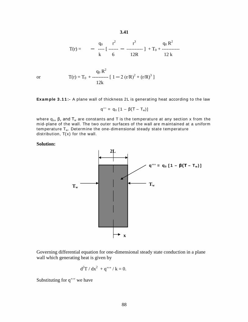
88
3.41 q0 r2 r3 q0 R2
T(r) = ─ ---- [ ------ ─ ---------- ] + T0 + ----------- k 6 12R 12 k q0 R2 or T(r) = T0 + ---------- [ 1 ─ 2 (r/R)2 + (r/R)3 ] 12k Example 3.11:- A plane wall of thickness 2L is generating heat according to the law q’’’ = q0 [1 – β(T – Tw)] where qo, β, and Tw are constants and T is the temperature at any section x from the mid-plane of the wall. The two outer surfaces of the wall are maintained at a uniform temperature Tw. Determine the one-dimensional steady state temperature distribution, T(x) for the wall. Solution:
Governing differential equation for one-dimensional steady state conduction in a plane wall which generating heat is given by d2T / dx2 + q’’’ / k = 0. Substituting for q’’’ we have
2L
x
Tw
Tw
q’’’ = q0 [1 – β(T – Tw)]
89
3.42 d2T / dx2 + qo [ 1 – β(T – Tw)] /k = 0 Defining a new variable θ = T – Tw, the above equation can be written as d2θ / dx2 + qo [ 1 – βθ] /k = 0 or d2θ / dx2 − qo βθ /k = qo / k or d2θ / dx2 − m 2θ = qo / k ……………………………..(1a) where m2 = q0 β /k ……………………………...(1b) Eq.(1a) is a second order linear non-homogeneous differential equation whose solution is given by θ (x) = θh(x) + θp(x) ………………………………….(2) where θh(x) satisfies the differential equation d2θh / dx2 − m 2θh = 0 ……………………………….(3) Solution to Eq.(3) is given by θh(x) = A1 e mx + A2 e − mx…………………………….(4) θp(x) satisfies the differential equation d2θp / dx2 − m 2θ p = qo / k…………………………..(5) The term qo/k makes the governing differential equation non-homogeneous. Since this is a constant θp(x) is also assumed to be constant. Thus let θp(x) = C, where C is a constant. Substituting this solution in Eq. (5) we get − m 2C = qo / k Or C = - qo /(km2) Substituting for m2 we get C = − 1 / β. Hence θp(x) = − 1 / β …………………………….(6) The complete solution θ(x) is therefore given by θ(x) = A1 e mx + A2 e − mx − 1 / β …………………..(7)

90
3.43
The constants A1 and A2 in Eq.(7) can be determined by using the two boundary conditions, which are: (i)at x = 0, dT / dx = 0 (axis of symmetry) i.e., dθ / dx = 0 (ii) at x = L, T = Tw ; i.e., θ = 0 From Eq.(7), dθ / dx = m[A1e mx – A2 e − mx ] Substituting condition (i) we get m[A1 – A2] = 0 Or A1 = A2.
Substituting condition (ii) in Eq.(7) we get A1[e mL + e − mL] = 1 / β (1 / β) Or A1 = ---------------------------- [e mL + e − mL] Substituting the expressions for A1 and A2 in Eq. (7) we get the temperature distribution in the plane wall as (1 / β ) θ(x) = T(x) – Tw = -------------------- [ e mx + e − mx ] − 1 / β [e mL + e − mL] 1 e mx + e − mx Or T(x) – Tw = ---- [ ----------------- − 1] β e mL + e − mL [e m(L – x) + e − m(L – x)] cosh m(L – x) or T(x) – Tw = (1 / β)---------------------------- = (1 / β)---------------------------- [e mL + e − mL] cosh mL 3.4. Critical Radius of Insulation:- For a plane wall adding more insulation will result in a decrease in heat transfer as the area of heat flow remains constant .But adding insulation to a cylindrical pipe or a conducting wire or a spherical shell will result in an increase in thermal resistance for conduction at the same will result in a decrease in the convection resistance of the outer surface because of increase in surface area for convection. Therefore the heat transfer may either increase or decrease depending on the relative magnitude of these two resistances. Critical Radius of Insulation for Cylinder:- Let us consider a cylindrical pipe of outer radius rs maintained at a constant temperature of Ts. Let the pipe now be insulated with

91
3.44 a material of thermal conductivity k and outer radius r. Let the outer surface of the insulation be in contact with a fluid at a uniform temperature T∞ with a surface heat transfer coefficient h. Then the thermal circuit for this arrangement will be as shown in Fig.3.15.
The rate of heat transfer from the pipe to the ambient is given by (Ts - T∞) (Ts – To) Q = ------------------ = ----------------------------------- …………………………...(3.44) [Rins + Rco] ln (r / rs) 1 ---------- + -------------- 2 π L k 2 π r L h It can be seen from Eq. (3.44) that if Ts and h are assumed not to vary with ‘r’ then Q depends only on r and the nature of variation of Q with r will be as shown in Fig.3.16. The value of r at which Q reaches a maximum can be determined as follows. (Ts – To) Eq. (3.44) can be written as Q = ----------- F(r) ln (r / rs) 1 where F(r) = ---------- + -------------- 2 π L k 2 π r L h Hence for Q to be maximum, F(r) has to be minimum: i.e., dF(r) / dr = 0
r
rs
Rins Rco Q Ts
T∞
Ts
Surface in contact with a fluid at T∞ and surface heat transfer coefficient h
Fig.3.15: Schematic of a cylindrical pipe covered with an insulation and exposed to an ambient and the corresponding thermal circuit
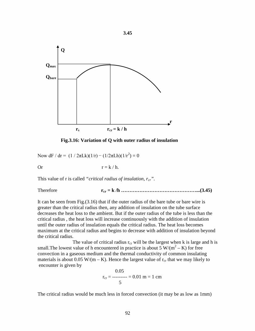
92
3.45
Now dF / dr = (1 / 2πLk)(1/r) − (1/2πLh)(1/r2) = 0 Or r = k / h. This value of r is called “critical radius of insulation, rcr”. Therefore rcr = k /h ………………………………………...(3.45) It can be seen from Fig.(3.16) that if the outer radius of the bare tube or bare wire is greater than the critical radius then, any addition of insulation on the tube surface decreases the heat loss to the ambient. But if the outer radius of the tube is less than the critical radius , the heat loss will increase continuously with the addition of insulation until the outer radius of insulation equals the critical radius. The heat loss becomes maximum at the critical radius and begins to decrease with addition of insulation beyond the critical radius. The value of critical radius rcr will be the largest when k is large and h is small.The lowest value of h encountered in practice is about 5 W/(m2 – K) for free convection in a gaseous medium and the thermal conductivity of common insulating materials is about 0.05 W/(m – K). Hence the largest value of rcr that we may likely to encounter is given by 0.05 rcr = --------- = 0.01 m = 1 cm 5 The critical radius would be much less in forced convection (it may be as low as 1mm)
r
Q
rs rcr = k / h
Qmax Qbare
Fig.3.16: Variation of Q with outer radius of insulation

93
3.46 because of large values of h associated with forced convection. Hence we can insulate hot water or steam pipes freely without worrying about the possibility of increasing the heat loss to the surroundings by insulating the pipes. The radius of electric wires may be smaller than the critical radius. Therefore, the plastic electrical insulation may enhance the heat transfer from electric wires, there by keeping their steady operating temperatures at lower and safer levels. Critical Radius Insulation for a Sphere:- The analysis described above for cylindrical pipes can be repeated for a sphere and it can be shown that for a sphere the critical radius of insulation is given by 2k rcr = ------- …………………………………..(3.46) h Example 3.12:-A conductor with 8 mm diameter carrying an electric current passes
through an ambient at 30 0 C with a convection coefficient of 120 W/(m2 – K). The temperature of the conductor is to be maintained at 130 0 C. Calculate the rate of heat loss per metre length of the conductor when (a) the conductor is bare and (b) conductor is covered with bakelite insulation [k = 1.2 W/(m-K)] with radius corresponding to the critical radius of insulation.
Solution:
(a) When the conductor is bare the rate of heat loss to the ambient is given by Q = h πD L (Ts - T∞) = 120 x π x 0.008 x 1 x (130 – 30) = 301.6 W/m. (b) When the conductor is covered with critical thickness of insulation,
Ts= 130 0 C
h = 120 W/(m2-K) T∞ = 30 0 C
D = 0.008 mm
(a) Conductor without Insulation.
Dc K = 1.2 W/(m-K)
h = 120 W/(m2 – K) T∞ = 30 0 C
Ts = 130 0 C
(b) Conductor with critical thickness of insulation

94
Dc = 2 rc = 2 (k/h) = 2 x ( 1.2 / 120) = 0.02 m. 1 1 R insulation = -------------- ln (Dc / D) = ----------------------- ln (0.02 / 0.008) 2π L k 2 π x 1.0 x 1.2 = 0.1215 (m – 0 C) / W. 1 1 Rco = 1 / (h Ac) = ---------------- = ------------------------ = 0.133 (m – 0 C)/W. π Dc L h π x 0.02 x 1 x 120 ∑R = Rinsulation + Rco = 0.1215 + 0.133 = 0.2545 (m – 0 C) / W.
(Ts - T∞) (130 – 30) Qinsulation
= ------------------- = --------------- = 392.93 W / m. ∑R 0.145 Example 3.13:-An electrical current of 700 A flows through a stainless steel cable
having a diameter of 5 mm and an electrical resistance of 6x10 ─ 4 ohms per metre length of the cable. The cable is in an environment at a uniform temperature of 30 0 C and the surface heat transfer coefficient of 25 W/(m2 – 0C). (a) What is the surface temperature of the cable when it is bare? (b)What thickness of insulation of k = 0.5 W/(m – K) will yield the lowest value of the maximum insulation temperature? What is this temperature when the thickness is used?
Solution: (a) When the cable is Bare: - Electrical Resistance = Re = 6 x 10 ─ 4 Ω / m Current through the cable = I = 700 A; D = 0.005 m ; h = 25 W/(m2-K) ; T∞ = 30 0 C. Power dissipated = Q = I2 Re = (700)2 x 6 x 10─ 4 = 294 W / m. But Q = hA(Ts - T∞) or Ts = T∞ + Q / [(πD L) x h] Or Ts = 30 + 294 / [(π x 0.005 x 1) x 25] = 779 0 C. (b) When the cable is covered with insulation: k = 0.5 W/(m-K) ; Hence critical radius = rc = k / h = 0.5 / 25 = 0.02 (m-K) / W. Thickness of insulation = rc – D/2 = 0.02 – 0.005 / 2 = 0.0175 m

95
3.48 1 1 Rinsulation = --------------- ln (rc / ro) = ------------------- ln (0.02 / 0.0025) = 0.662 (m-K)/W (2π L k) (2π x 1 x 0.5) 1 1 Rco = 1 / (hAo) = ------------------- = ------------------------------ = 0.318 (m-K) / W. (2π rcL h) (2 x π x 0.02 x 1 x 25) (Ts - T∞) Q = --------------------- or Ts = T∞ + Q (Rinsulation + Rco) Rinsulation + Rco Or Ts = 30 + 294 x (0.662 + 0.318) = 318.12 0 C. Example 3.14:- A 2 mm-diameter and 10 m-long electric wire is tightly wrapped With a 1 mm-thick plastic cover whose thermal conductivity is 0.15 W / (m-K). Electrical measurements indicate that a current of 10 A passes through the wire and there is a voltage drop of 8 V along the wire. If the insulated wire is exposed to a medium at 30 0C with a heat transfer coefficient of 24 W / (m2 – K), determine the temperature at the interface of the wire and the plastic cover in steady operation. Also determine if doubling the thickness of the plastic cover will increase or decrease this interface temperature. Given: Outer radius of the bare wire = rs = 1 mm = 0.001 m ; Length of the wire = L = 10 m ; outer radius of plastic insulation = r = 1 + 1 = 2 mm = 0.002 m ; Current through the wire = I = 10 A ; Voltage drop in the wire = V = 8 V ; Ambient temperature = T∞ = 30 0C ; Thermal conductivity of the plastic cover = k = 0.15 W /(m– K) ; Surface heat transfer coefficient = h = 24 W /(m2 – K). To find: (i) Interface temperature = Ts ; (ii) Whether Ts increases or decreases when the thickness of insulation is doubled. Solution: (i) Q = VI = 8 x 10 = 80 W. The thermal circuit for the problem is shown in Fig. P3.14. ln (r / rs) ln ( 0.002 / 0.001) Rins = ------------ = ----------------------------- = 0.0735 K / W 2 π L k 2 x π x 10 x 0.15 1 1 1 Rco = -------------- = -------------- = ------------------------------ = 0.3316 K / W h Ao 2 π L r h 2 x π x 10 x 0.002 x 24
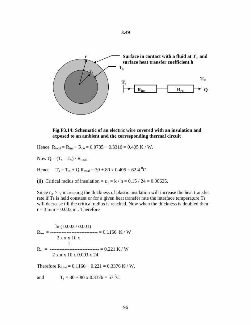
96
3.49
Hence Rtotal = Rins + Rco = 0.0735 + 0.3316 = 0.405 K / W. Now Q = (Ts - T∞) / Rtotal.
Hence Ts = T∞ + Q Rtotal = 30 + 80 x 0.405 = 62.4 0C (ii) Critical radius of insulation = rcr = k / h = 0.15 / 24 = 0.00625. Since rcr > r, increasing the thickness of plastic insulation will increase the heat transfer rate if Ts is held constant or for a given heat transfer rate the interface temperature Ts will decrease till the critical radius is reached. Now when the thickness is doubled then r = 3 mm = 0.003 m . Therefore ln ( 0.003 / 0.001) Rins = ----------------------------- = 0.1166 K / W 2 x π x 10 x 1 Rco = ------------------------------ = 0.221 K / W 2 x π x 10 x 0.003 x 24 Therefore Rtotal = 0.1166 + 0.221 = 0.3376 K / W. and Ts = 30 + 80 x 0.3376 = 57 0C
r
rs
Rins Rco Q Ts
T∞
Ts
Surface in contact with a fluid at T∞ and surface heat transfer coefficient h
Fig.P3.14: Schematic of an electric wire covered with an insulation and exposed to an ambient and the corresponding thermal circuit
97
3.50 3.5. Extended Surfaces (Fins):- Solution to tutorial problems: Example 3.15:- A steel rod of diameter 2 cm and thermal conductivity 50 W/(m – K) is exposed to ambient air at 20 0C with a heat transfer coefficient 64 W/(m2 – K). One end of the rod is maintained at a uniform temperature of 120 0C. Determine the rate of heat from the rod to the ambient and the temperature of the tip of the rod exposed to ambient if (i) the rod is very long, (ii) rod is of length 10 cm with negligible heat loss from its tip, (ii) rod is of length 25 cm with heat loss from its tip. Solution: (i) Given:- D = 0.02 m ; k = 50 W/(m-K); T∞ = 20 0C; To = 120 0C; h = 64 W/(m2-K); Very long fin (x → ∞) m = √ [(hP) / (kA) = √ [(hπD / (πD2/4)] = √[(4h) / (kD)] 4 x 64 = √ [ --------------------------- ] = 16 50 x 0.02 For a very long fin the rate of heat transfer is given by Q = kmA(T0 - T∞) = 50 x 16 x (π / 4) x 0.022 x [ 120 – 20] = 25.13 W (ii) L = 0.10 m. Hence mL = 16 x 0.1 = 1.6 Q = kmA(T0 - T∞) tanh mL = 50 x 16 x (π / 4) x 0.022 x (120 – 20) x tanh 1.6 = 23.16 W (iii) When the heat loss from the rod tip is not negligible, then we can use the same formula as in case (ii) with modified length Le given by Le = L + A /P = L + (πD2/4) /(πD) = L + D / 4 = 0.1 + 0.02/4 = 0.105 Hence mLe = 16 x 0.105 = 1.68 and tanh mLe = tanh 1.68 = 0.9329 Hence Q = 25.13 x 0.933 = 23.44 W Example 3.16:-A thin rod of uniform cross section A, length L and thermal
conductivity k is thermally attached from its ends to two walls which are maintained at temperatures T1 and T2. The rod is dissipating heat from its lateral surface to an ambient at temperature T∞ with a surface heat transfer coefficient h.
98
3.51 (a) Obtain an expression for the temperature distribution along the length of the
rod (b) Also obtain an expression for the heat dissipation from the rod to the ambient
Solution: The general solution for the one-dimensional steady-state temperature distribution along the length of a rod dissipating heat by convection from its lateral surface is given by θ(x) = C1 cosh mx + C2 sinh mx ………………………..(1) ___________ where θ(x) = T(x) - T∞ ; m = √ (hP) / (kA) : P = perimeter of the rod = π D and A = Area of cross section of the rod = π D2 / 4.
The boundary conditions are: (i) at x = 0, T = T1 or θ = T1 - T∞ = θo (say). (ii) at x = L, T = T2 or θ = T2 - T∞ = θL (say). Condition(i) in Eq. (1) gives θo = C1. Condition (ii) in Eq. (1) gives θL = θ0 cosh mL + C2 sinh mL (θL ─ θo cosh mL) C2 = ------------------------ . sinh mL Substituting for C1 and C2 in Eq. (1) we have (θL ─ θo cosh mL) θ(x) = θo cosh mx + ------------------------ sinh mx sinh mL θo cosh mx sinh mL + θL sinh mx ─ θo cosh mL sinh mx 0r θ(x) = ------------------------------------------------------------------------ sinh mL θL sinh mx + θo sinh m(L – x) 0r θ(x) = -------------------------------------- ……………………………………..(2) sinh mL Expression for the rate of heat dissipation from the rod:

99
─ m [θL + θ0 cosh mL] Therefore (dθ / dx)|x = 0 = ------------------------------- sinh mL ─ m [θL cosh mL + θ0] and (dθ / dx)|x = L = ------------------------------ sinh mL kmA [θL + θ0 cosh mL ─ θL cosh mL ─ θ0 ] Hence Qamb = --------------------------------------------------------- sinh mL kmA [(θL – θ0) ─ (θL ─ θ0) cosh mL ] = ---------------------------------------------------------- sinh mL kmA(θL – θ0) (1 ─ cosh mL) or Qamb = ------------------------------------- sinh mL Example 3.17:-Heat is generated at a constant rate of q’’’ W/m3 in a thin circular
rod of length L and diameter D by the passage of electric current. The two ends of the rod are maintained at uniform temperatures with one end at temperature T0 and the other end at 0 0 C, while heat is being dissipated from the lateral surface of the rod to an ambient at 0 0C with a surface heat transfer coefficient h.
(a) Derive the one-dimensional steady state energy equation to determine the temperature distribution along the length of the rod
(b) Solve the above equation and obtain the temperature distribution.
L
x
Q |x=L Q|x=0
Qamb
Energy balance for the rod is given by Q amb = Q |x = 0 ─ Q |x = L = ─ kA (dθ / dx)|x = 0 + kA (dθ / dx)|x = L ……………………………(3) ─ m [θLcosh mx + θ0 cosh m(L – x)] From Eq. (2) we have (dθ / dx) = -------------------------------------------------- sinh mL
3.52
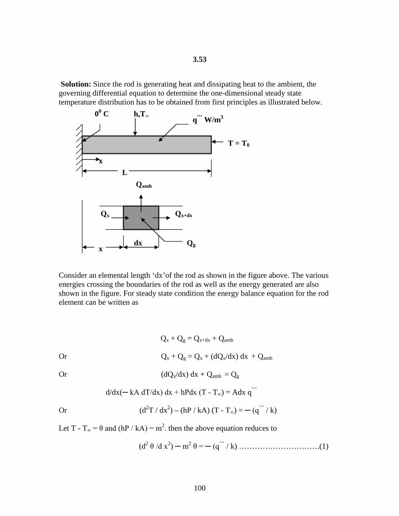
100
3.53
Solution: Since the rod is generating heat and dissipating heat to the ambient, the governing differential equation to determine the one-dimensional steady state temperature distribution has to be obtained from first principles as illustrated below.
Consider an elemental length ‘dx’of the rod as shown in the figure above. The various energies crossing the boundaries of the rod as well as the energy generated are also shown in the figure. For steady state condition the energy balance equation for the rod element can be written as
Qx + Qg = Qx+dx + Qamb
Or Qx + Qg = Qx + (dQx/dx) dx + Qamb
Or (dQx/dx) dx + Qamb = Qg
d/dx(─ kA dT/dx) dx + hPdx (T - T∞) = Adx q’’’ Or (d2T / dx2) – (hP / kA) (T - T∞) = ─ (q’’’ / k) Let T - T∞ = θ and (hP / kA) = m2. then the above equation reduces to (d2 θ /d x2) ─ m2 θ = ─ (q’’’ / k) ………………………….(1)
00 C h,T∞
T = T0
q’’’ W/m3
x L
dx x
Qx Qx+dx
Qamb
Qg
101
3.54 Eq.(1) is a non-homogeneous linear second order ordinary differential equation whose solution can be written as θ(x) = θh(x) + θp(x) ------------------------------------(2) where θh(x) satisfies the homogeneous part of the differential equation namely (d2 θh /d x2) ─ m2 θh = 0 -------------------------------------(3) and θp(x) is the particular integral which satisfies Eq. (1). Solution to Eq.(3) is given by θ(x) = C1 e mx + C2 e ─ mx -----------------------------(4) To find θp(x) :- Since the RHS of Eq.(1) is a constant let us assume θp(x) = B, where B is a constant. Substituting this solution in Eq.(1) we have 0 – m2 B = ─ (q’’’ / k) Or B = (q’’’ / km2) Therefore the complete solution for Eq. (1) can be written as θ(x) = C1 e mx + C2 e ─ mx + (q’’’ / km2) Or T(x) = T∞ + C1 e mx + C2 e ─ mx + (q’’’ / km2)………………..(5) Boundary conditions are: (i) at x = 0, T = 0 (ii) at x = L, T = T0
Condition (i) in Eq. (5) gives 0 = T∞ + C1 + C2 + (q’’’/ km2) Or C1 + C2 = ─ T∞ ─ (q’’’/km2) ------------------------------- (a) Condition(ii) in Eq.(5) gives T0 = T∞ + C1 e mL + C2 e ─ mL + (q’’’/km2) Or C1 e mL + C2 e ─ mL = T0 ─ T∞ ─ (q’’’/km2) ----------------------------- (b) From Eq.(a) C2 = ─ C1 ─ T∞ ─ (q’’’/km2). Substituting this expression in Eq.(b) we have C1 e mL ─ [C1 + T∞ + (q’’’/km2)] e ─ mL = T0 ─ T∞ ─ (q’’’/km2)

102
3.55
T0 ─ {T∞ + (q’’’/km2)}{1 ─ e ─ mL } Solving for C1 we get C1 = -------------------------------------------------- { e mL ─ e ─ mL } T0 ─ {T∞ + (q’’’/km2)}{1 ─ e ─ mL } C2 = ─{ T∞ + (q’’’/km2) }─ -------------------------------------------------- { e mL ─ e ─ mL } ─{ T∞ + (q’’’/km2) }{ e mL ─ e ─ mL } ─ T0 + {T∞ + (q’’’/km2)}{1 ─ e ─ mL } C2 = ------------------------------------------------------------------------------------------------ { e mL ─ e ─ mL } { T∞ + (q’’’/km2) }[ ─ e mL + e ─ mL + 1 ─ e ─ mL] ─ T0 C2 = ----------------------------------------------------------------------------------------------- { e mL ─ e ─ mL } { T∞ + (q’’’/km2) }[ 1 ─ e mL] ─ T0 C2 = ---------------------------------------------- { e mL ─ e ─ mL } Substituting the expressions for C1 and C2 in Eq. (5) and simplifying we get [T0 ─ {T∞ + (q’’’/km2)}{1 ─ e ─ mL }] e mx
T(x) = T∞ + (q’’’/km2) + ------------------------------------------------- { e mL ─ e ─ mL } [ { T∞ + (q’’’/km2) }[ 1 ─ e mL] ─ T0] e ─ mx + ---------------------------------------------------- { e mL ─ e ─ mL }
T0(e mx - e ─ mx) T(x) = T∞ + (q’’’/km2) + --------------------- + { e mL ─ e ─ mL } [ ─{T∞ + (q’’’/km2)}{ 1 ─ e ─ mL }] e mx + { T∞ + (q’’’/km2) }[ 1 ─ e mL] e ─ mx] ---------------------------------------------------------------------------------------------- { e mL ─ e ─ mL } Example 3.18:- Two very long slender rods of the same diameter are given. One
rod is of aluminum (k = 200 W/(m-K)). The thermal conductivity of the other

103
3.56
rod is not known. To determine this, one end of each rod is thermally attached to a metal surface maintained at a uniform temperature T0. Both
rods are losing heat to the ambient air at T∞ by convection with a surface heat transfer coefficient h. The surface temperature of each rod is measured at various distances from hot base surface. The temperature of the aluminum rod at 40 cm from the base is same as that of the rod of unknown thermal conductivity at 20 cm from the base. Determine the unknown thermal conductivity.
Solution:
For rod A Eq.(1) can be written as θa(x) = θ0 e ─ ma xa …………………………...(2) And for rod B it can be written as θb(x) = θ0 e ─ mb xb ……………………………(3) It is given that when xa = 0.4 m and xb = 0.2 m, θa(xa) = θb(xb) Therefore we have θ0 e ─ 0.4 ma = θ0 e ─ 0.2 mb Or mb = 2 ma Or √ [(hPb) / (kbAb)] = 2√[ (hPa) / (kaAa)] Since Pa = Pb and Aa = Ab, we have √ ka = 2 √ kb or ka = 4 kb
Therefore kb = 200/4 = 50 W/(m-K).
xa
xb
ka = 200 W/(m-K)
kb = ?
Ta
Tb = Ta
For very long slender rods the steady-state one-dimensional temperature distribution along the length of the rod is given by θ (x) = θ0 e ─ mx ……………………………..(1) where θ(x) = T(x) - T∞ and θ0 = T0
- T∞.
104
3.57 Example 3.19:- Show that for a finned surface the total heat transfer rate is given by Qtotal = [η β + (1 – β)] a h θ0 = ή a h θ0
Where η = fin efficiency ; β= af / a : af = surface area of the fin, a = total heat transfer area (i.e. finned surface + unfinned surface) ; θ0 = T0 - T∞, with T0 = fin base temperature and T∞ = ambient temperature, and ή = area – weighted fin efficiency.
Solution: Qtotal = Qfin + Qbare Where Qtotal = Total heat transfer rate, Qfin = Heat transfer rate from the finned surface and Qbare = Heat transfer rate from the bare surface. Therefore Qtotal = η h af θ0 + h(a – af) θ0 = h a θ0 [(η af) / a + (1 – af/a)] here, β= af/a = ha θ0 [ηβ + (1 – β)] = ή ha θ0 , where ή = [ηβ + (1 – β)] Example 3.20:- The handle of a ladle used for pouring molten lead at 327 0 C is 30 cm long and is made of 2.5 cm x 1.5 cm mild steel bar stock (k = 43 W/(m-K)). In order to reduce the grip temperature, it is proposed to make a hollow handle of mild steel plate 1.5 mm thick to the same rectangular shape. If the surface heat transfer coefficient is 14.5 W/(m2-K) and the ambient temperature is 27 0C, estimate the reduction in the temperature of the grip. Neglect the heat transfer from the inner surface of the hollow shape. Solution: (a) When the handle is made of solid steel bar:

105
3.58
Therefore mL = 8.48 x 0.3 = 2.54. When the heat loss from the tip of the handle is neglected the temperature at any point along the length of the handle is given by cosh m(L – x) θ(x) = θ0
---------------------- cosh mL
Therefore θ(x)|x=L = θ0 / cosh mL = 300 / cosh 2.54 = 47 0 C.
Or T(x)|x=L = 47 + 27 = 74 0 C. (b) When the handle is hollow made out of a sheet:
2.5 cm
1.5 cm
h = 14.5 W/(m2-K) ; k = 43 W/(m-K) θ0 = 327 – 27 = 300 0 C
Area of cross section of the bar = A = 2.5 x 1.5 x 10 ─ 4 m2 = 3.75 x 10 ─ 4 m2
Perimeter of the bar = P = 2 [ 2.5 + 1.5] x 10 ─ 2 m = 8 x 10 ─ 2 m ( hP)(1/2) √ [14.5 x 8 x 10 ─ 2] Therefore m = ------ = -------------------------- = 8.48 (1/m) (kA)(1/2) √[43 x 3.75 x 10 ─ 4]
Cross section of the handle

106
3.59
Or m = 15.59 1/m. Therefore mL = 15.59 x 0.3 = 4.68 θ0 (327 – 27) θ(x)|x=L = -------------------- = ----------------- = 5.57 0 C. cosh mL cosh 4.68 Therefore T(x)|x=L = 5.57 + 27 = 32.57 0 C. Reduction in grip temperature = 74 – 32.57 = 41.43 0 C. Example 3.21:- Derive an expression for the overall heat transfer coefficient across a plane wall of thickness ‘b’ and thermal conductivity ‘k’ having rectangular fins on both sides. Given that over an overall area A of the wall, the bare area on both sides, not covered by the fins are Au1 and Au2, the fin efficiencies are η1 and η2, and the heat transfer coefficients h1 and h2. Solution: Let Ti be the temperature of the fluid in contact with the surface 1, T0 be the temperature of the fluid in contact with surface 2, T1 be the temperature of surface 1 and T2 be the temperature of surface 2.Let Ti >T0. Then the rate of heat transfer from Ti to T0 is given by Q = Qbare + Q fin = hiAu1 (Ti – T1) + hi η1Af1(Ti – T1)
2.5 cm
1.5 cm
1.5 mm thick
Area of the cross section of the fin is A = [(2.5 x 1.5) – (2.5 – 0.3) x (1.5 – 0.3)] = 1.11 cm 2 = 1.11 x 10 − 4 m2 P = 2 x [ 2.5 + 1.5 ] = 8 cm = 8 x 10 − 2 m _________ √(14.5 x 8 x 10 − 2) m = √(hP) / (kA) = ---------------------------- √( 43 x 1.11 x 10 − 4)

107
3.60
(Ti – T1) (Ti – T1) Or Q = --------------- − ------------------- (1 /h1Au1) (1/h1η1Af1) (Ti – T1) Q = ------------------ ---------------- …………………………(1) [(1 /h1Au1) + (1/h1η1Af1) ] (T2 – T0) Q = ------------------ ---------------- …………………………(2) [(1 /h2Au2) + (1/h2η2Af2) ] Rate of heat transfer is also given by (T1 – T2) Q = ---------------- …………………………………………(3) (b/Ak) Therefore as A/B = C/D = E/F = (A+C+E)/(B+D+F) (Ti – T1) + (T1 – T2) + (T2 – T0) Q = -------------------------------------------------------------------------- [(1 /h1Au1) + (1/h1η1Af1) + (1 /h1Au1) + (1/h1η1Af1) +(b/Ak)] (Ti – T0) Q = -------------------------------------------------------------------------- ……(4) [(1 /h1Au1) + (1/h1η1Af1) + (1 /h1Au1) + (1/h1η1Af1) +(b/Ak)] If U = overall heat transfer coefficient for the plane wall then Q = UA(Ti – T0) (Ti – T0) = ----------------- ………………………………….(5) (1/UA) From Eqs. (4) and (5) we have 1 U = ------------------------------------------------------------------------------ A [(1 /h1Au1) + (1/h1η1Af1) + (1 /h1Au1) + (1/h1η1Af1) +(b/Ak)]

108
3.61
Example 3.22:- Calculate the effectiveness of the composite pin fin shown in
Fig.P3.22. Assume k1 = 15 W/(m-K), k2 = 50 W/(m-K) and h = 12 W/(m2 – K). Solution:
Energy balance equation for the fin element is given by Qx = Qx+dx + Qc = Qx + (dQx/dx) dx + Qc Or dQx / dx + Qc = 0 ………………………………………..(1) Qx consists of two components namely the heat transfer Qx1 through the material of thermal conductivity k1 and the rate of heat transfer Qx2 through the material of conductivity k2. Therefore Qx = Qx1 + Qx2 = − k1A1 (dT / dx) − k2A2 (dT / dx) = − (k1A1 + k2A2) (dT / dx) And Qc = (hP2 dx) (T - T∞). Substituting these expressions for Qx and Qc in equation (1) we get
3 mm = d1
d2 = 10 mm k1
k2
L
dx
Qx Qx+dx
Qc K1=15 W/m-k , K2=50W/m-k, K3=12 W/m-k. (b) Energy transfer across the surfaces of the fin element
x

109
3.62
hP2 (d2T / dx2) − ------------------- (T – T∞) = 0 (k1A1 + k2A2)
Or (d2θ / dx2) − m2 θ = 0 …………………………(2) Where θ = T – T∞ and m = √ [ hP2 / (k1A1 + k2A2) ]. When the heat loss from the fin tip is negligible , the solution to equation (2) is given by cosh [m(L – x)] θ(x) = θ0 ---------------------- ………..(3) cosh mL The rate of heat transfer from the fin base is given by Qx|x=0 = − (k1A1 + k2A2) (dθ / dx)|x=0 − (k1A1 + k2A2) sinh [m(L – x)]x=0 (- m) θ0 = ---------------------------------------------------- cosh mL = mθ0 (k1A1 + k2A2) tanh mL Now η = Qx|x=0 / Qmax mθ0 (k1A1 + k2A2) tanh mL = ---------------------------------------- hP2L θ0 Noting that hP2 / (k1A1 + k2A2) = m2, the above expression for η simplifiers to tanh mL η = ------------------------ ……………………(4) mL In the given problem A1 = (π / 4) x (0.003)2 = 7.1 x 10 − 6 m2. A2 = (π / 4) x [ (0.01)2 – (0.003)2] = 7.15 x 10 − 5 P2 = π x 0.01 0.0314 m.
110
3.63
√ [ 12 x 0.0314] m = ----------------------------------------------------- = 10.12 √[(15 x 7.1 x 10 − 6 ) + (50 x 7.15 x 10 − 5)] Therefore mL = 10.12 x 0.1 = 1.012
tanh (1.012) η = ------------------ = 0.757 1.012 Example 3.23:- Why is it necessary to derive a fresh differential equation for
determining the one-dimensional steady state temperature distribution along the length of a fin?
Solution:- While deriving the conduction equation in differential form we will have considered a differential volume element within the solid so that the heat transfer across the boundary surfaces of the element is purely by conduction. But in the case of a fin the lateral surface is exposed to an ambient so that the heat transfer across the lateral surfaces is by convection. Therefore we have to derive the differential equation afresh taking into account the heat transfer by convection across the lateral surfaces of the fin. Solutions to Problems on Conduction in solids with variable thermal conductivity Example 3.24:- A plane wall 4 cm thick has one of its surfaces in contact with a fluid at 130 0C with a surface heat transfer coefficient of 250 W/(m2 – K) and the other surface is in contact with another fluid at 30 0C with a surface heat transfer coefficient of 500 W/(m2-K). The thermal conductivity of the wall varies with temperature according to the law k = 20 [ 1 + 0.001 T] where T is the temperature. Determine the rate of heat transfer through the wall and the surface temperatures of the wall. Given:- L = 0.04 m; Ti = 130 0C; hi = 250 W/(m2-k); To = 30 0C; ho = 500 W/(m2-K); k = 20 [ 1 + 0.001 T]. To find:- (i) Qx (ii) T1 and T2 Solution: Rci = Thermal resistance for convection at the surface at Ti = 1/(hiA) = 1 / (250 x 1) = 0.004 m2 – K /W Rco = Thermal resistance for convection at the surface at To = 1/(hoA) = 1/(500 x 1)
111
3.64 Or Rco = 0.002 m2-K/W Now Q = (Ti – T1) / Rci, where T1 = Surface temperature in contact with fluid at Ti. Hence T1 = Ti – QRci = 130 – 0.004 Q ………………………………………….(1) Similarly Q = (T2 – To) / Rco Or T2 = To + QRco = 30 + 0.002Q ……………………………………………(2) From equations (1) and (2) we have T1 – T2 = 100 – 0.006Q ………………………………………………………….(3) And Tm = ( T1 + T2) / 2 = 80 – 0.001Q ...……………………………………….(4) Hence km = ko [ 1 + βTm] = 20 x [1 + 0.001x {80 – 0.001Q}] = 21.6 – 2 x 10 − 5Q Hence thermal resistance offered by the wall = R = L/(Akm) 0.04 Or R = --------------------------- [21.6 – 2 x 10 − 5Q] [T1 – T2] [100 – 0.006Q] [21.6 – 2 x 10 − 5Q] Q = --------------------- = ---------------------------x -------------------------- R 0.04 Cross multiplying we have 0.04Q = 2160 – 0.1316Q + 1.2 x 10 − 7 Q2
Or Q2 – 1.41 x 10 6 Q + 1.8 x 10 10 = 0.Hence Q = (1.41 x 10 6 ±1.39 x 10 6) / 2 For physically meaningful solution T1 should lie between Ti and To. This is possible only If Q = (1.41 x 10 6 − 1.39 x 10 6) / 2 = 10000 W. Now T1 = Ti – QRci = 130 – 10000 x 0.004 = 90 0C and T2 = T0 + Q Rco = 30 + 10000 x 0.002 = 50 0C.

112
3.65 Example 3.25:- The thermal conductivity of a plane wall varies with
temperature according to the equation k(T) = k0 [ 1 + β T2 ] where k0 and β are constants.
(a) Develop an expression for the heat transfer through the wall per unit area of the wall if the two surfaces are maintained at temperatures T1 and T2 and the thickness of the wall is L.
(b) Develop a relation for the thermal resistance of the wall if the heat transfer area is A.
Solution:
L T2 ∫Qxdx = − k0A ∫[1 +βT2]dT
0 T1
Or QxL = − k0A [(T2 – T1) + (β/3)(T23 – T1
3)] Or Qx = (k0A / L)(T1 – T2) [1 + (β/3)(T1
2 +T1T2 + T22)]
(T1 – T2) Qx = ------------------------------------------------------- 1 --------------------------------------------------- (k0A/L) [1 + (β/3)(T1
2 +T1T2 + T22)]
Therefore thermal resistance of the wall is given by
x
T1 T2
K = k0 [ 1 + βT2]
L
For steady state conduction we have Qx = − kA(dT / dx) = constant. Or Qx = − k0[1 +βT2]A(dT/dx) Qxdx = − k0[1 +βT2]A dT Integrating the above equation between x = 0 and x = L we have
L

113
3.66 1 R = --------------------------------------------------- (k0A/L) [1 + (β/3)(T1
2 +T1T2 + T22)]
Example 3.26:- Find the steady-state heat flux through the composite slab made up of two materials as shown in Fig. P 3.26. Also find the interfacial temperature. The thermal conductivities of the two materials vary linearly with the temperature in the following manner: k1 = 0.05 [1 + 0.008 T] W/m-K and k2 = 0.04 [1 + 0.0075 T] W/m-K
10 cm 5 cm
k1 k2
600 0 C 30 0 C
Fig. P 3.26: Schematic for problem 3.26
L2 L1
k1 k2 T1
T3 T2
Data:- T1 = 600 0 C ; T2 = 30 0 C ; L1 = 0.05 m ; L2 = 0.10 m ; k1 = 0.05 [ 1 + 0.008T ] ; k2 = 0.04 [ 1 + 0.0075T ] To find T3 and q
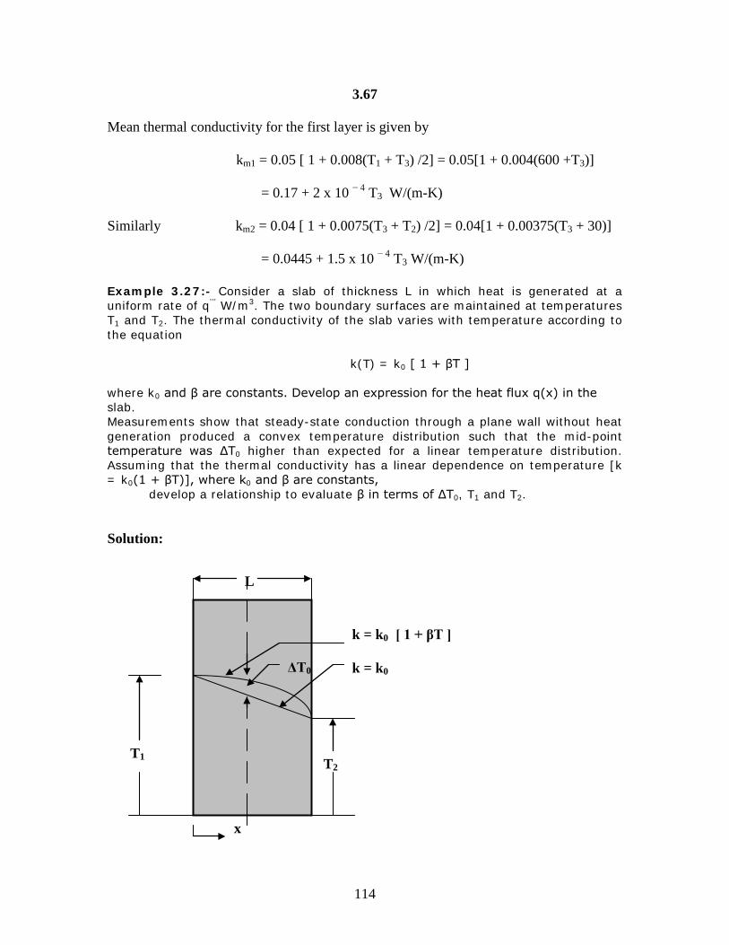
114
3.67 Mean thermal conductivity for the first layer is given by km1 = 0.05 [ 1 + 0.008(T1 + T3) /2] = 0.05[1 + 0.004(600 +T3)] = 0.17 + 2 x 10 − 4 T3 W/(m-K) Similarly km2 = 0.04 [ 1 + 0.0075(T3 + T2) /2] = 0.04[1 + 0.00375(T3 + 30)] = 0.0445 + 1.5 x 10 − 4 T3 W/(m-K) Example 3.27:- Consider a slab of thickness L in which heat is generated at a uniform rate of q’’’ W/m3. The two boundary surfaces are maintained at temperatures T1 and T2. The thermal conductivity of the slab varies with temperature according to the equation k(T) = k0 [ 1 + βT ] where k0 and β are constants. Develop an expression for the heat flux q(x) in the slab. Measurements show that steady-state conduction through a plane wall without heat generation produced a convex temperature distribution such that the mid-point temperature was ΔT0 higher than expected for a linear temperature distribution. Assuming that the thermal conductivity has a linear dependence on temperature [k = k0(1 + βT)], where k0 and β are constants, develop a relationship to evaluate β in terms of ΔT0, T1 and T2. Solution:
L
T1 T2
ΔT0
k = k0 [ 1 + βT ] k = k0
x
115
3.68
For constant thermal conductivity k0, the temperature distribution in the wall is linear and is given by T(x) = T1 – (T1 – T2) x / L Therefore T(x)|x=L/2 = (T1 + T2) / 2 ……………………………………….(1) When the thermal conductivity varies with temperature the temperature distribution in the wall is determined as follows. Qx = − kA(dT/dx) = − k0(1 + βT)A (dT/dx) Therefore Qx dx = − k0A(1 + βT) dT ……………………………………..(2) Integrating the above equation between x = 0 and any x at which the temperature is given by T*(x) we have x T* ∫Qxdx = ∫− k0A(1 + βT) dT
0 T1
Or Qx x = − k0A [(T* - T1) + (β/2)(T*2 – T12)] ……………(3)
If equation is integrated between x = 0 and x = L we get Qx L = − k0A [(T2 - T1) + (β/2)(T2
2 – T12)]
Or Qx = (k0A)[1 + β(T1 + T2) / 2] (T1 – T2) / L Or Qx = kmA (T1 – T2) / L ……………………………………….(4) Where km = k0 [1 + β(T1 + T2) / 2]. Substituting this expression for Qx in equation (3) we get km (T1 – T2) (x / L) = − k0[(T* - T1) + (β/2)(T*2 – T1
2)] The above equation simplifies to T*2 + (2/β)T* + [ (2/β){(km/k0)(T1 – T2)(x/L) – T1} – T1
2 ] = 0. Therefore

116
3.69 ___________________________________________ T* = − (1/β) ± √ (1/β2) – (2km / βk0)(x / L)(T1 – T2) + T1
2 + (2 / β)T1 _____________________________________ T*|x=L/2 = − (1/β) ± √ (1/β2) – (km / βk0)(T1 – T2) + T1
2 + (2 / β)T1 __________________________________________________ = − (1/β) ± √ (1/β2) – [k0{1 + β(T1 + T2)/2}/ βk0](T1 – T2) + T1
2 + (2 / β)T1 _______________________________________________ = − (1/β) ± √ (1/β2) – [{1 + β(T1 + T2)/2}/β ](T1 – T2) + T1
2 + (2 / β)T1 But T*|x=L/2 = T(x)|x=L/2 + ΔT0 = (T1 + T2) / 2 + ΔT0. Hence we have ______________________________________________ (T1 + T2)/2 +ΔT0 = − (1/β) ± √ (1/β2) – [{1 + β(T1 + T2)/2}/β ](T1 – T2) + T1
2 + (2 / β)T1 Example 3.28:- A slab of thickness ‘L’ has its two surfaces at x=0 and x = L maintained at uniform temperatures of T0 and TL respectively. The thermal conductivity of the slab has spatial variation according to the law k = k0 [1 + α x], where ko and α are constants. Obtain expressions for (i) temperature distribution in the slab, and (ii) rate of heat transfer through the slab assuming one dimensional steady state conduction. Solution:
The governing differential equation for one dimensional steady state conduction without heat generation is given by
x
T1 T2
k = k0 [1 + α x]
L
Fig. E3.28 : Figure for Example 3.28

117
3.70 d / dx [k dT/dx] = 0 substituting for k we have d / dx [k0 (1 + α x) dT/dx] = 0 ………………………………..(1) Let 1 + α x = y ; Then α dx = dy or dy/dx = α. Then Eq.(1) can be written in terms of the variable ‘y’ as follows. {d / dy [k0 y (dT/dy) α ] }α = 0. Or {d / dy [k0 y (dT/dy) α ] } = 0 Integrating w.r.t ‘y’ once we get [k0 y (dT/dy) α ] = C1
Or dT = [C1 /(α k0)] (dy / y) Integrating once we have, T = [C1 /(α k0)] ln y + C2 Substituting for ‘y’ in terms of ‘x’ we have T = [C1 /(α k0)] ln (1 + α x) + C2 ………………..(2) Eq.(2) is the general solution of Eq.(1). The values of C1 and C2 can be obtained from the two boundary conditions at x = 0 and at x = L as follows.
(i) at x = 0, T = T1; and (ii) at x = L, T = T2 ; Condition (i) in Eq. (2) gives T1 = C2; Condition (ii) in Eq. (20 gives T2 = [C1 /(α k0)] ln (1 + α L) + T1 Or C1 = (T2 – T1) (α k0) / ln (1 + α L) . Substituing the values of C1and C2 in Eq.(2) we get the temperature distribution as: T(x) = (T2 – T1) ln ((1 + α x) / ln (1 + α L) + T1 Expression for rate of heat transfer: At any ‘x’ Qx = - k A (dT/dx)
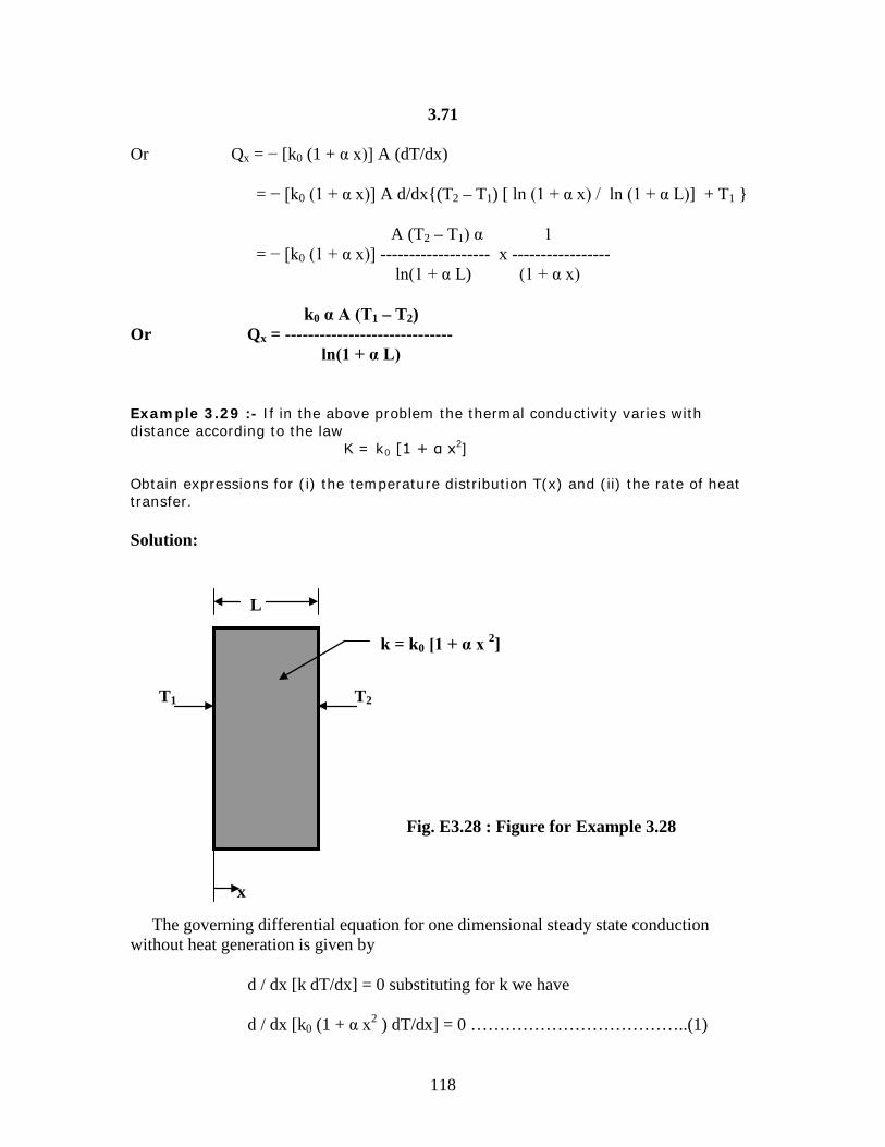
118
3.71 Or Qx = − [k0 (1 + α x)] A (dT/dx) = − [k0 (1 + α x)] A d/dx{(T2 – T1) [ ln (1 + α x) / ln (1 + α L)] + T1 } A (T2 – T1) α 1 = − [k0 (1 + α x)] ------------------- x ----------------- ln(1 + α L) (1 + α x) k0 α A (T1 – T2) Or Qx = ----------------------------- ln(1 + α L) Example 3.29 :- If in the above problem the thermal conductivity varies with distance according to the law K = k0 [1 + α x2] Obtain expressions for (i) the temperature distribution T(x) and (ii) the rate of heat transfer. Solution:
The governing differential equation for one dimensional steady state conduction without heat generation is given by d / dx [k dT/dx] = 0 substituting for k we have d / dx [k0 (1 + α x2 ) dT/dx] = 0 ………………………………..(1)
x
T1 T2
k = k0 [1 + α x 2]
L
Fig. E3.28 : Figure for Example 3.28

119
3.72
Eq. (2) can be solved by using the following substitution. Let √α x = tan y. Differnatiating both sides w.r.t.’x’ we have √α = sec 2 y (dy/dx) √α or (dy/dx) = √α / sec 2 y = ------------------- . [ 1 + α x2 ] Or [ 1 + α x2 ] (dy / dx) = √α. Eq. (1) can be written in terms of variable ‘y’ as d / dy[k0 (1 + α x2) (dy/dx) (dT/dy)] (dy/dx) = 0 Substituting for (1 + α x2) (dy/dx) we get d/ dy [k0 √α (dT/dy)] [√α / sec 2 y] = 0. Or d/ dy [k0 √α (dT/dy)] = 0. Integrating w.r.t.’y’ we have, k0 √α (dT / dy) = C1 Or dT = [C1 /( k0 √α)] dy. Integrating we get T = [C1/ (k0 √α )] y + C2
Or T(x) = [C1/(k0 √α)] tan −1(√α x) + C2 ………………………….(3) Boundary conditions are: (i) at x = 0 T (x) = T1 and (ii) at x = L ,T = T2. Condition (i) in Eq. (3) gives C2 = T1.
Condition (ii) in Eq. (3) gives T2 = [C1/(k0 √α)] tan −1(√α L) + T1
[T2 – T1]k0 √α Or C1 = ------------------ tan −1(√α L) Substituting the values of C1 and C2 we have tan −1 (√α x) T(x) = [T2 – T1] ----------------- tan −1 (√α L)

120
3.73 Expression for Rate of Heat Transfer: Qx = − k0 [1 + α x2] A (dT/dx) √α = − k0 [1 + α x2] A [T2 – T1] --------------------------- [1 + α x2] tan −1 (√α L) k0 A √α [T1 – T2] Or Qx = ------------------------------- tan −1 (√α L) Example 3.30:- A hollow cylinder has its internal surface at radius r1 maintained at a uniform temperature T1 and external surface at radius r2 maintained at a uniform temperature T2. The thermal conductivity of the material of the cylinder varies with radius according to the law k = k0 [1 + α r], where k0 and α are constants. Derive expressions for (i) radial temperature distribution in the cylinder and (ii) rate of heat transfer through the cylinder. Assume one-dimensional radial steady state conduction in the cylinder. Example 3.31:- A hollow cylinder has its internal surface at radius r1 maintained at a uniform temperature T1 and external surface at radius r2 maintained at a uniform temperature T2. The thermal conductivity of the material of the cylinder varies with radius according to the law k = k0 [1 + α r2], where k0 and α are constants. Derive expressions for (i) radial temperature distribution in the cylinder and (ii) rate of heat transfer through the cylinder. Assume one-dimensional radial steady state conduction in the cylinder. Example 3.32:- A hollow sphere has its internal surface at radius r1 maintained at a uniform temperature T1 and external surface at radius r2 maintained at a uniform temperature T2. The thermal conductivity of the material of the cylinder varies with radius according to the law k = k0 [1 + α r], where k0 and α are constants. Derive expressions for (i) radial temperature distribution in the cylinder and (ii) rate of heat transfer through the cylinder. Assume one-dimensional radial steady state conduction in the cylinder. Example 3.33:- A hollow sphere has its internal surface at radius r1 maintained at a uniform temperature T1 and external surface at radius r2 maintained at a uniform temperature T2. The thermal conductivity of the material of the cylinder varies with radius according to the law k = k0 [1 + α r2], where k0 and α are constants. Derive expressions for (i) radial temperature distribution in the cylinder and (ii) rate of heat transfer through the cylinder. Assume one-dimensional radial steady state conduction in the cylinder.

121
Chapter 4
Transient Conduction
4.1.Introduction:- In general, the temperature of a body varies with time as well as position.In chapter 3 we have discussed conduction in solids under steady state conditions for which the temperature at any location in the body do not vary with time. But there are many practical situations where in the surface temperature of the body is suddenly altered or the surface may be subjected to a prescribed heat flux all of a sudden. Under such circumstances the temperature at any location within the body varies with time until steady state conditions are reached. In this chapter, we take into account the variation of temperature with time as well as with position.However there are many practical applications where in the temperature variation with respect to the location in the body at any instant of time is negligible. The analysis of such heat transfer problems is called the “lumped system analysis”. Therefore in lumped system analysis we assume that the temperature of the body is a function of time only. 4.2. Lumped system analysis:- Consider a solid of volume V, surface area A, density ρ, Specific heat Cp and thermal conductivity k be initially at a uniform temperature Ti.Suddenly let the body be immersed in a fluid which is maintained at a uniform temperature T∞, which is different from Ti.The problem is illustrated in Fig.4.1.Now if
V = volume A=surface area ρ = density Cp = specific heat k = conductivity
Surface in contact with fluid at T∞ with surface heat transfer Coefficient h
Fig.4.1: Nomenclature for lumped system analysis of transient Conduction heat transfer

122
4.2 T(t) is the temperature of the solid at any time t, then the energy balance equation for the solid at time t can be written as Rate of increase of energy of the solid = Rate of heat transfer from the fluid to the solid i.e., ρVCp (dT / dt ) = hA[T∞ - T(t)] h A Or dT / dt = ---------- [T∞ − T(t)] ρ V Cp For convenience, a new temperature θ(t) = T(t) - T∞ is defined and denoting m = (hA)/(ρVCp) the above equation can be written as (dθ /dt ) = − m θ ………………………………………..(4.1) Eq.(4.1) is a first order linear differential equation and can be solved by separating the variables. Thus dθ / θ = − m dt Integrating we get ln θ = − mt + ln C, where ln C is a constant.
Or θ = C e − mt ………………………………………...(4.2) At time t = 0 , T(t) = Ti or θ = Ti − T∞ = θi (say). Substituting this condition in Eq. (4.2) we get C = θi. Substituting this value of C in eq. (4.2) we get the temperature θ(t) as follows. θ(t) = θi e − mt or θ(t) ----- = e – mt …………………………………………(4.3) θi Since LHS of Eq.(4.3) is dimensionless, it follows that 1/m has the dimension of time and is called the time constant.Fig. 4.2 shows the plot of Eq.(4.3) for different values of m. Two observations can be made from this figure and Eq. (4.3).
1. Eq. (4.3) can be used to determine the temperature T(t) of the solid at any time t or to determine the time required by the solid to reach a specified temperature.

123
4.3
2. The plot shows that as the value of m increases the solid approaches the surroundings temperature in a shorter time.That is any increase in m will cause the solid to respond more quickly to approach the surroundings temperature.
The definition of m reveals that increasing the surface area for a given volume and the heat transfer coefficient will increase m. Increasing the density, specific heat or volume decreases m. 4.2.2.Criteria for Lumped System Analysis:- To establish a criterion to neglect internal temperature gradient of the solid so that lumped system analysis becomes applicable, a Characteristic length Ls is defined as Ls = V /A …………………………………(4.4) and the Biot. number Bi as h Ls Bi = --------- ……………………………..(4.5) k For solids like slabs, infinite cylinder, and sphere, it has been found that the error by neglecting internal temperature gradients is less than 5 %, if Bi < 0.1 ……………………………………(4.6) The physical significance of Biot number can be understood better by writing the expression for Biot number as follows
t
θ(t) θi
1.0
Fig.4.2: Dimensionless temperature as a function of time for a solid with negligible internal temperature gradients
m
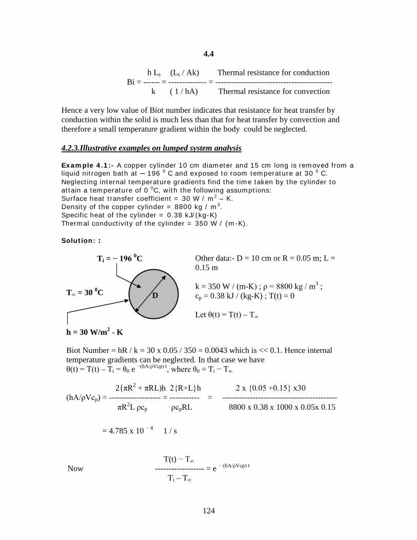
124
4.4 h Ls (Ls / Ak) Thermal resistance for conduction Bi = ------ = -------------- = ------------------------------------------- k ( 1 / hA) Thermal resistance for convection Hence a very low value of Biot number indicates that resistance for heat transfer by conduction within the solid is much less than that for heat transfer by convection and therefore a small temperature gradient within the body could be neglected. 4.2.3.Illustrative examples on lumped system analysis Example 4.1:- A copper cylinder 10 cm diameter and 15 cm long is removed from a liquid nitrogen bath at ─ 196 0 C and exposed to room temperature at 30 0 C. Neglecting internal temperature gradients find the time taken by the cylinder to attain a temperature of 0 0C, with the following assumptions: Surface heat transfer coefficient = 30 W / m2 – K. Density of the copper cylinder = 8800 kg / m3. Specific heat of the cylinder = 0.38 kJ/(kg-K) Thermal conductivity of the cylinder = 350 W / (m-K). Solution: :
= 4.785 x 10 − 4 1 / s T(t) − T∞ Now ------------------ = e − (hA/ρVcp) t Ti – T∞
D
Ti = − 196 0C
h = 30 W/m2 - K
T∞ = 30 0C
Other data:- D = 10 cm or R = 0.05 m; L = 0.15 m k = 350 W / (m-K) ; ρ = 8800 kg / m3 ; cp = 0.38 kJ / (kg-K) ; T(t) = 0 Let θ(t) = T(t) – T∞
Biot Number = hR / k = 30 x 0.05 / 350 = 0.0043 which is << 0.1. Hence internal temperature gradients can be neglected. In that case we have θ(t) = T(t) – Ti = θ0 e −(hA/ρVcp) t, where θ0 = Ti − T∞ 2{πR2 + πRL)h 2{R+L}h 2 x {0.05 +0.15} x30 (hA/ρVcp) = ------------------- = ----------- = ------------------------------------------
πR2L ρcp ρcpRL 8800 x 0.38 x 1000 x 0.05x 0.15

125
4.5 0 − 30 Hence ------------------- = exp (− 4.785 x 10 − 4 x t) − 196 – 30 Solving for t we get t = 4226 s = 1 hr 10.43 mins. Example 4.2:- A thin copper wire having a diameter D and length L (insulated at the ends) is initially at a uniform temperature of T0. Suddenly it is exposed to a gas stream, the temperature of which changes with time according to the equation Tg = Tf (1 ─ e─ ct) + T0 where Tf, T0 and c are constants. The surface heat transfer coefficient is h. Obtain an expression for the temperature of the wire as a function of time t. Solution: Let T(t) be the temperature of the cylinder at any time t. Energy balance for the cylinder for a time interval dt is given by hA [T∞ - T(t)] dt = ρVCp dT where dT is the increase in temperature of the cylinder in time dt.
dT / dt + m T(t) = m [T0 + Tf (1 – e - ct)] or dT / dt + m [T(t) – T0] = mTf (1 – e – ct )
L
D
T(0) = T0
h,T∞
Or dT / dt = (hA/ρVCp) [T∞ - T(t)] Putting m = (hA/ρVCp), the above equation reduces to dT / dt + m T(t) = m T∞ Substituting the given expression for T∞ we have
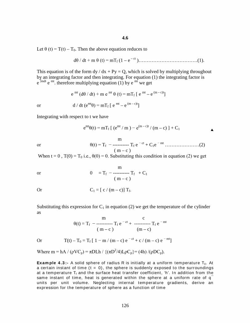
126
4.6
Let θ (t) = T(t) – T0. Then the above equation reduces to dθ / dt + m θ (t) = mTf (1 – e – ct )………………………………(1). This equation is of the form dy / dx + Py = Q, which is solved by multiplying throughout by an integrating factor and then integrating. For equation (1) the integrating factor is e ∫mdt e mt. therefore multiplying equation (1) by e mt we get e mt (dθ / dt) + m e mt θ (t) = mTf [ e mt – e (m – c)t] or d / dt (emtθ) = mTf [ e mt – e (m – c)t] Integrating with respect to t we have emtθ(t) = mTf [ (emt / m ) − e(m – c)t / (m – c) ] + C1 m or θ(t) = Tf − ---------- Tf e − ct + C1e − mt …………………(2) ( m – c ) When t = 0 , T(0) = T0 i.e., θ(0) = 0. Substituting this condition in equation (2) we get m or 0 = Tf − ---------- Tf + C1 ( m – c ) Or C1 = [ c / (m – c)] Tf. Substituting this expression for C1 in equation (2) we get the temperature of the cylinder as m c θ(t) = Tf − ---------- Tf e − ct + ---------- Tf e − mt ( m – c ) (m – c) Or T(t) – T0 = Tf [ 1 − m / (m – c) e − ct + c / (m – c) e − mt] Where m = hA / (ρVCp) = πDLh / {(πD2/4)LρCp}= (4h) /(ρDCp). Example 4.3:- A solid sphere of radius R is initially at a uniform temperature T0. At a certain instant of time (t = 0), the sphere is suddenly exposed to the surroundings at a temperature Tf and the surface heat transfer coefficient, ‘h’. In addition from the same instant of time, heat is generated within the sphere at a uniform rate of q’’’ units per unit volume. Neglecting internal temperature gradients, derive an expression for the temperature of sphere as a function of time

127
4.7
Solution:
Multiplying equation (1) by the integrating factor e mt we have emt (dθ / dt) + emt mθ = q0 emt or d / dt(θemt) = q0emt
Integrating throughout w.r.t. t we get θemt = (q0 / m) emt + C1 or θ = (q0
/ m) + C1e − mt …………………...(2) At t = 0 , T = T0 or θ = T0 – Tf = θ0 (say). Substituting this condition in equation (2) we get C1 = (T0 – Tf) – (q0 / m). Therefore the temperature in the sphere as a function of time is given by θ(t) = [(T0 – Tf) – (q0 / m)] e − mt + (q0 / m) or θ(t) = (q0 / m)[ 1 – e − mt ] + (T0 – Tf) e − mt
R
T(0) = T0
Q``` for t > 0
h,Tf
Energy balance equation for the sphere at any time t can be written as (4/3)πR3 q’’’ + 4πR2h [Tf – T(t)] =(4/3)πR3 ρCp (dT/dt)
Or (dT/dt) + (3h/ ρRCp)[T(t) – Tf] = (q```/ρCp) Let θ(t) = T(t) – Tf. Then the above equation reduces to (dθ / dt) + mθ = q0 ………………………………..(1) Where m = (3h/ ρRCp) and q0 = (q```/ρCp)

128
4.8 q’’’ (ρ R Cp) where (q0 / m) = ----------- x --------------- = (q’’’ R / 3h) (ρ Cp) 3h Example 4.4:- A solid steel ball (ρ =8000 kg/m3 ; cp = 0.42 kJ/kg-K) 5 cm in diameter is at a uniform temperature of 450 0 C. It is quenched in a controlled environment which is initially at 90 0C and whose temperature increases linearly with time at the rate of 10 0C per minute. If the surface heat transfer coefficient is 58 W/(m2-K), determine the variation of the temperature of the ball with time neglecting internal temperature gradients. Find the value of the minimum temperature to which the ball cools and the time taken to reach this minimum temperature. Solution:
Or (dT / dt) = (hA/ ρVCp) [Tf(t) – T(t)] Letting m = (hA/ ρVCp) the above equation can be written as (dT / dt) + mT(t) = m Tf(t)
Substituting for Tf(t) from equation (1) we have (dT / dt) + mT(t) = m [90 + t / 6 ] Multiplying the above equation with the integrating factor e mt we get
R
T(0) = Ti = 4500C
h,Tf
Other data:- h = 58 W / (m2 – K) ; Cp = 0.42 kJ / (kg – K) ; ρ = 8000 kg / m3 ; Tf = a + bt, where a and b are constants ; at t = 0, Tf = 90 0C;(dTf / dt) = 10 0C / min = (1/6) 0 C / s
Therefore a = 90 0 C and b = ;(dTf / dt) = (1/6) 0 C / s. Or Tf = 90 + t / 6 , t in seconds……………….(1) Energy balance equation for the sphere at any time t can be written as ρVCp(dT / dt) = hA [Tf(t) – T(t)]
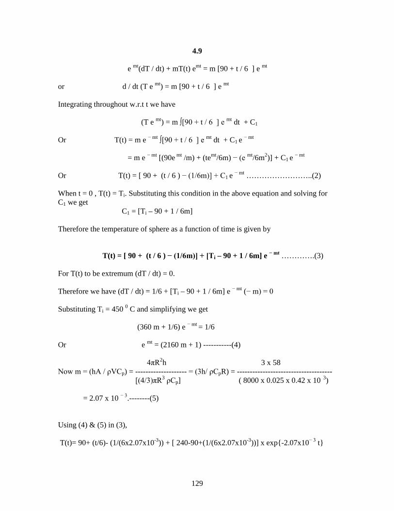
129
4.9 e mt(dT / dt) + mT(t) emt = m [90 + t / 6 ] e mt or d / dt (T e mt) = m [90 + t / 6 ] e mt Integrating throughout w.r.t t we have (T e mt) = m ∫[90 + t / 6 ] e mt dt + C1 Or T(t) = m e − mt ∫[90 + t / 6 ] e mt dt + C1 e − mt = m e − mt [(90e mt /m) + (temt/6m) − (e mt/6m2)] + C1 e − mt Or T(t) = [ 90 + (t / 6 ) − (1/6m)] + C1 e − mt ……………………..(2) When t = 0 , T(t) = Ti. Substituting this condition in the above equation and solving for C1 we get C1 = [Ti – 90 + 1 / 6m] Therefore the temperature of sphere as a function of time is given by T(t) = [ 90 + (t / 6 ) − (1/6m)] + [Ti – 90 + 1 / 6m] e − mt ………….(3) For T(t) to be extremum (dT / dt) = 0. Therefore we have (dT / dt) = 1/6 + [Ti – 90 + 1 / 6m] e − mt (− m) = 0 Substituting Ti = 450 0 C and simplifying we get (360 m + 1/6) e − mt = 1/6 Or e mt = (2160 m + 1) -----------(4) 4πR2h 3 x 58 Now m = (hA / ρVCp) = -------------------- = (3h/ ρCpR) = ------------------------------------- [(4/3)πR3 ρCp] ( 8000 x 0.025 x 0.42 x 10 3) = 2.07 x 10 − 3.--------(5)
Using (4) & (5) in (3), T(t)= 90+ (t/6)- (1/(6x2.07x10-3)) + [ 240-90+(1/(6x2.07x10-3))] x exp{-2.07x10− 3 t}
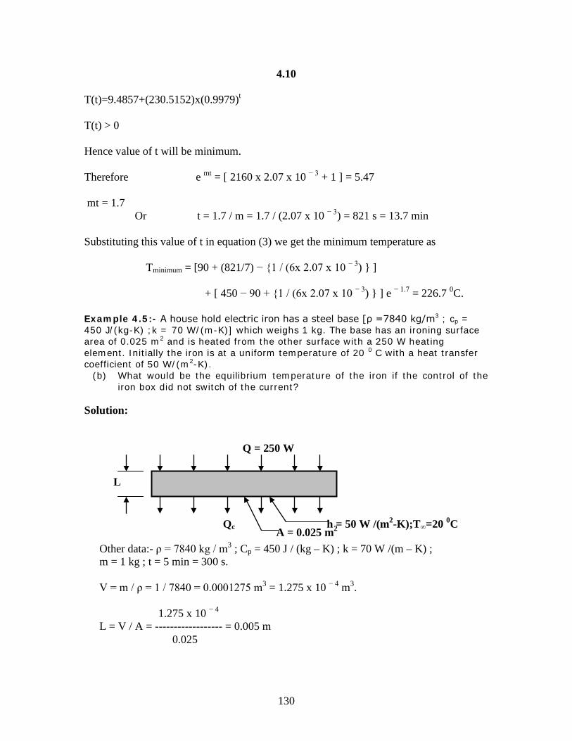
130
4.10 T(t)=9.4857+(230.5152)x(0.9979)t
T(t) > 0 Hence value of t will be minimum. Therefore e mt = [ 2160 x 2.07 x 10 − 3 + 1 ] = 5.47 mt = 1.7 Or t = 1.7 / m = 1.7 / (2.07 x 10 − 3) = 821 s = 13.7 min Substituting this value of t in equation (3) we get the minimum temperature as Tminimum = [90 + (821/7) − {1 / (6x 2.07 x 10 − 3) } ] + [ 450 − 90 + {1 / (6x 2.07 x 10 − 3) } ] e − 1.7 = 226.7 0C. Example 4.5:- A house hold electric iron has a steel base [ρ =7840 kg/m3 ; cp = 450 J/(kg-K) ;k = 70 W/(m-K)] which weighs 1 kg. The base has an ironing surface area of 0.025 m2 and is heated from the other surface with a 250 W heating element. Initially the iron is at a uniform temperature of 20 0 C with a heat transfer coefficient of 50 W/(m2-K).
(b) What would be the equilibrium temperature of the iron if the control of the iron box did not switch of the current?
Solution:
L
Qc
Q = 250 W
h = 50 W /(m2-K);T∞=20 0C A = 0.025 m2
Other data:- ρ = 7840 kg / m3 ; Cp = 450 J / (kg – K) ; k = 70 W /(m – K) ; m = 1 kg ; t = 5 min = 300 s. V = m / ρ = 1 / 7840 = 0.0001275 m3 = 1.275 x 10 − 4 m3. 1.275 x 10 − 4 L = V / A = ------------------ = 0.005 m 0.025
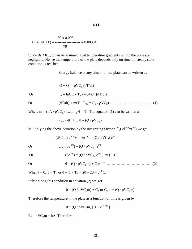
131
4.11 50 x 0.005 Bi = (hL / k) = -------------------- = 0.00364 70 Since Bi < 0.1, it can be assumed that temperature gradients within the plate are negligible. Hence the temperature of the plate depends only on time till steady state condition is reached. Energy balance at any time t for the plate can be written as
Q − Qc = ρVCp (dT/dt) Or Q – hA(T - T∞) = ρVCp (dT/dt) Or (dT/dt) + m(T - T∞) = (Q / ρVCp) ……………………………..(1) Where m = (hA / ρVCp). Letting θ = T - T∞, equation (1) can be written as (dθ / dt) + m θ = (Q / ρVCp) Multiplying the above equation by the integrating factor e mt,( e∫mdt=emt) we get (dθ / dt) e mt + m θe mt = (Q / ρVCp) emt Or d/dt (θe mt) = (Q / ρVCp) emt Or (θe mt) = (Q / ρVCp) emt (1/m) + C1 Or θ = (Q / ρVCpm) + C1e − mt ……………………………….(2) When t = 0, T = Ti or θ = Ti - T∞ = 20 – 20 = 0 0 C. Substituting this condition in equation (2) we get 0 = (Q / ρVCpm) + C1 or C1 = − (Q / ρVCpm) Therefore the temperature in the plate as a function of time is given by θ = (Q / ρVCpm) [ 1 − e − mt ] But ρVCpm = hA. Therefore

132
4.12 θ = (Q / hA) [ 1 − e − mt ] …………………………………..(3) 250 50 x 0.025 Q / hA = ------------------- = 200 ; m = ------------------- = 2.8 x 10⁻³
50 x 0.025 1 x 450 Therefore θ = 200 [ 1 – e −0.028t] When t = 300 s, θ = T - T∞ = 200 x [ 1 − e − 0.028 x 300] = 113.7
Or T = 113.7 + 20 = 133.7 0 C. (b) When the control switch is not switched off and the iron is left in the ambient, steady state condition will be attained as t tends to ∞ so that the heat transferred to the baseplate will be convected to the ambient. i.e., Q = Qc Therefore 250 = 50 x 0.025 x [T – 20 ] Or T = 220 0 C. This answer can also be obtained by putting t = ∞ in equation (3) and solving for T. 4.3 One-dimensional Transient Conduction ( Use of Heissler’s Charts): There are many situations where we cannot neglect internal temperature gradients in a solid while analyzing transient conduction problems. Then we have to determine the temperature distribution within the solid as a function of position and time and the analysis becomes more complex. However the problem of one-dimensional transient conduction in solids without heat generation can be solved readily using the method of separation of variables.The analysis is illustrated for solids subjected to convective boundary conditions and the solutions were presented in the form of transient – temperature charts by Heissler. These charts are now familiarly known as “Heissler’s charts”. 4.3.1.One-dimensional transient conduction in a slab:- Let us consider a slab of thickness 2L, which is initially at a uniform temperature Ti. Suudenly let the solid be exposed to an environment which is maintained at a uniform temperature of T∞ with a surface heat transfer coefficient of h for time t > 0.Fig.4.3 shows the geometry , the coordinates and the boundary conditions for the problem. Because of symmetry in the problem with respect to the centre of the slab the ‘x’ coordinate is measured from the centre line of the slab as shown in the figure.
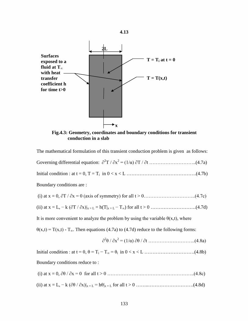
133
4.13
The mathematical formulation of this transient conduction problem is given as follows: Governing differential equation: ∂2T / ∂x2 = (1/α) ∂T / ∂t ………………………..(4.7a) Initial condition : at t = 0, T = Ti in 0 < x < L …………………………………….(4.7b) Boundary conditions are : (i) at x = 0, ∂T / ∂x = 0 (axis of symmetry) for all t > 0…………………………..(4.7c) (ii) at x = L, − k (∂T / ∂x)|x = L = h(T|x = L − T∞) for all t > 0 ……………………….(4.7d) It is more convenient to analyze the problem by using the variable θ(x,t), where θ(x,t) = T(x,t) - T∞. Then equations (4.7a) to (4.7d) reduce to the following forms: ∂2θ / ∂x2 = (1/α) ∂θ / ∂t ………………………..(4.8a) Initial condition : at t = 0, θ = Ti − T∞ = θi in 0 < x < L ………………………….(4.8b) Boundary conditions reduce to : (i) at x = 0, ∂θ / ∂x = 0 for all t > 0 ………………….…………………………..(4.8c) (ii) at x = L, − k (∂θ / ∂x)|x = L = hθ|x = L for all t > 0 ……..……………………….(4.8d)
x
2L
T = Ti at t = 0
T = T(x,t)
Surfaces exposed to a fluid at T∞ with heat transfer coefficient h for time t>0
Fig.4.3: Geometry, coordinates and boundary conditions for transient conduction in a slab

134
4.14
Eq.(4.8a) can be solved by the method of separation of variables as shown below. Let θ(x,t) = X(x) Y(t) ……………………………………………………………..(4.9) Substituting this in Eq. (4.8a) we get Y (d2X / dx2) = (X/α) (dY / dt) Or 1 1 --- (d2X / dx2) = ------ (dY / dt) …………………….(4.10) X (Yα) LHS of Eq. (4.10) is a function of x only and the RHS of Eq. (4.10) is a function of t only.They can be equal only to a constant say − λ 2.(The reason to choose the negative sign is to get a physically meaningful solution as explained later in this section).Hence we have two equations namely (1 / X) (d2X / dx2) = − λ2 and [1/(Yα)] ((dY / dt) = − λ2 Or (d2X / dx2) + λ2X = 0 ………………………………………………….(4.11) and (dY/dt) = −αλ2 Y ………………………………………………………(4.12) Solution to Eq. (4.11) is X(x) = C1 cos (λx) + C2 sin (λx) …………………….(4.13) and solution to Eq. (4.12) is Y(t) = D exp (− αλ2t) ………………………..(4.14) with C1, C2 and D as constants of integration. Substituting these solutions in Eq.(4.9) we have θ(x,t) = D exp (− αλ2t) [C1 cos (λx) + C2 sin (λx)] or θ(x,t) = exp (− αλ2t) [A1 cos (λx) + A2 sin (λx)]………..(4.15) Eq.(4.15) is the general solution involving the constants A1, A2 and λ which can be determined using the two boundary conditions and the initial condition as illustrated below. Now from Eq. (4.15), ∂θ / ∂x = λ exp (− αλ2t) [ −A1 sin (λx) + A2 cos (λx)] Substituting boundary condition (i) we have 0 = λ exp (− αλ2t) [0 + A2] for all t. Hence A2 = 0. Therefore Eq. (4.15) reduce to

135
4.15 θ(x,t) = A1 exp (− αλ2t) cos (λx) ……………………….(4.16) Now θ(L,t) = A1 exp (− αλ2t) cos (λL) and ∂θ / ∂x = λ exp (− αλ2t) [ −A1 sin (λx) ] Hence [∂θ / ∂x ] x = L = −λ A1 exp (− αλ2t) sin (λL) Therefore boundary condition (ii) can be written as k λ A1 exp (− αλ2t) sin (λL) = h A1 exp (− αλ2t) cos (λL) or tan (λL) = h / (kλ) or λL tan (λL) = Bi ……………………………………………(4.17) where Bi = hL / k. Equation (4.17) is called the “characteristic equation” and has infinite number of roots namely λ1, λ2, λ3, ..............Corresponding to each value of λ we have one solution and hence there are infinite number of solutions. Sum of all these solutions will also be a solution as the differential equation is linear. Therefore the solution θ(x,t) can be written as follows. θ(x,t) = ∑ An exp (− αλn 2t) cos (λnx) …………………….(4.18) To find An:- The constants An in Eq. (4.18) can be found using the orthogonal property of trigonometric functions as shown below.Substituting the initial condition we have θi = ∑ An cos (λnx) Multiplying both sides of Eq.(4.18) by cos λmx and integrating w.r.t ‘x’ between the limits 0 and L we have L L ∫ θi cos (λmx) dx = ∫ ∑ An cos (λmx) cos (λnx) dx
1 1
Using the orthogonal; property ∫ An cos (λmx) cos (λnx) dx = 0 for λn ≠ λm
The above equation reduce to L L ∫ θi cos (λnx) dx = ∫ An cos 2(λnx) dx
0 0
L θi 0 ∫cos (λnx) dx Or An = ----L------------------- ∫ cos 2 (λnx)dx 0

136
4.16 It is very convenient to express Eq. (4.18) in dimension less form as follows: θ(x,t) ----- = ∑ (An
* exp (− λn* 2 Fo) cos (λn* x / L) ………………………………(4.19)
θi where An
* = An / θi ; λn* = λnL ; Fo = Fourier Number = α t / L2 ;
4.3.2.Heissler’s Charts for transient conduction:- For values of Fo > 0.2 the above series solution converges rapidly and the solution will be accurate within 5 % if only the first term in the series is used to determine the temperature. In that case the solution reduces to θ(x,t) ----- = A1
* exp (− λ1* 2 Fo) cos (λ1* x /L) ……………………………………(4.20)
θi From the above equation the dimensionless temperature at the centre of the slab (x =0) can be written as θ(0,t)
----- = A1* exp (− λ1
* 2 Fo) ………………………………………………….(4.21) θi The values of A1
* and λ1* for different values of Bi are presented in the form of a table
(See Table 4.1). These values are evaluated using one term approximation of the series solution.It can also be concluded from Eq.(4.20) at any time ‘t’ the ratio θ(x,t) / θ(0,t) will be independent of temperature and is given by θ(x,t) ------ = cos (λ1* x /L) ……………………………………………………………(4.22) θ(0,t) Heissler has represented Eq. (4.21) and (4.22) in the form of charts and these charts are normally referred to as Heissler’s charts. Eq. (4.21) is plotted as Fourier number Fo versus dimensionless centre temperature θ(0,t) / θi using [Fig.4.4(b)]. reciprocal of Biot number1 / Bi as the parameter [Fig.4.4(a)], where as Eq. (4.22) is plotted as θ(x,t) / θ(0,t) versus reciprocal of Biot number using the dimensionless distance x / L as the parameter.In Fig.[4.4(a)], the curve for 1/Bi = 0 corresponds to the case h → ∞, or the outer surfaces of the slab are maintained at the ambient temperature T∞. For large values of 1 / Bi, the Biot number is small, or the internal conductance is large in comparison with the surface heat transfer coefficient. This in turn, implies that the temperature distribution within the solid is sufficiently uniform and hence lumped system analysis becomes applicable.
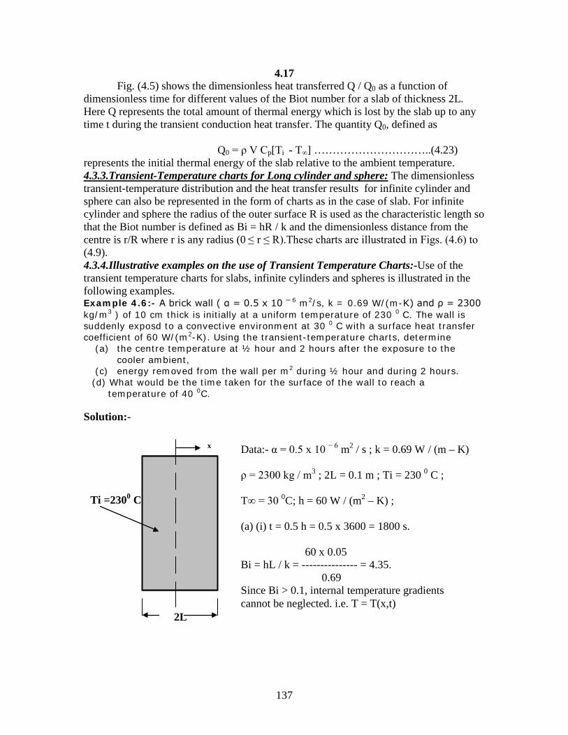
137
4.17 Fig. (4.5) shows the dimensionless heat transferred Q / Q0 as a function of dimensionless time for different values of the Biot number for a slab of thickness 2L. Here Q represents the total amount of thermal energy which is lost by the slab up to any time t during the transient conduction heat transfer. The quantity Q0, defined as Q0 = ρ V Cp[Ti - T∞] …………………………..(4.23) represents the initial thermal energy of the slab relative to the ambient temperature. 4.3.3.Transient-Temperature charts for Long cylinder and sphere: The dimensionless transient-temperature distribution and the heat transfer results for infinite cylinder and sphere can also be represented in the form of charts as in the case of slab. For infinite cylinder and sphere the radius of the outer surface R is used as the characteristic length so that the Biot number is defined as Bi = hR / k and the dimensionless distance from the centre is r/R where r is any radius (0 ≤ r ≤ R).These charts are illustrated in Figs. (4.6) to (4.9). 4.3.4.Illustrative examples on the use of Transient Temperature Charts:-Use of the transient temperature charts for slabs, infinite cylinders and spheres is illustrated in the following examples. Example 4.6:- A brick wall ( α = 0.5 x 10 ─ 6 m2/s, k = 0.69 W/(m-K) and ρ = 2300 kg/m3 ) of 10 cm thick is initially at a uniform temperature of 230 0 C. The wall is suddenly exposd to a convective environment at 30 0 C with a surface heat transfer coefficient of 60 W/(m2-K). Using the transient-temperature charts, determine
(a) the centre temperature at ½ hour and 2 hours after the exposure to the cooler ambient,
(c) energy removed from the wall per m2 during ½ hour and during 2 hours. (d) What would be the time taken for the surface of the wall to reach a temperature of 40 0C.
Solution:-
2L
x Data:- α = 0.5 x 10 − 6 m2 / s ; k = 0.69 W / (m – K) ρ = 2300 kg / m3 ; 2L = 0.1 m ; Ti = 230 0 C ; T∞ = 30 0C; h = 60 W / (m2 – K) ; (a) (i) t = 0.5 h = 0.5 x 3600 = 1800 s. 60 x 0.05 Bi = hL / k = --------------- = 4.35. 0.69 Since Bi > 0.1, internal temperature gradients cannot be neglected. i.e. T = T(x,t)
Ti =2300 C

138
4.18
Hence Heissler’s transient temperature charts are to be used. ( 0.5 x 10 − 6 x 1800)
1/ Bi = 1 / 4.35 = 0.23 ; Fo = (αt / L2) = -------------------------- = 0.36 2 From the Heissler’s chart for a slab of thickness 2L,
(T0 - T∞) θ0 = --------------- = 0.8 (T0 = Centre temperature of the slab) (Ti - T∞) Therefore T0 = T∞ + 0.8 (Ti - T∞) = 30 + 0.8 x (230 – 30) =190 0 C. (0.5 x 10 − 6 x 7200) (ii) when t = 2 h = 7200 s we have Fo = ---------------------------- = 1.44. (0.052) (T0 – T∞) From chart, -------------- = 0.125. (Ti – T∞) Therefore T0 = T∞ + 0.125 (T0 – T∞) = 30 + 0.125 x (230 – 30)= 55 0 C. (b) (i) t = 1800 s. At the surface x / L = 1.0 ; k / hL = 0.23 ; (T|x=L – T∞) Hence from the chart ---------------- = 0.275 (T0 – T∞) Or T|x=L = T∞ + 0.275 (T0 – T∞) = 30 + 0.275 x (190 – 30) = 74 0 C. (ii) t = 7200 s. Hence T|x=L = T∞ + 0.275 (T0 – T∞) = 30 + 0.275 x (55 – 30) = 36.9 0 C. (c) (i) Bi2 Fo = 4.35 2 x 0.36 = 6.81; From chart Q / Qmax = 0.50 . 0.69 x 1 x 0.1 Qmax = ρCpV(Ti – T∞) = (k / α)V(Ti – T∞) = ------------------- x (230 – 30) x 10 − 6
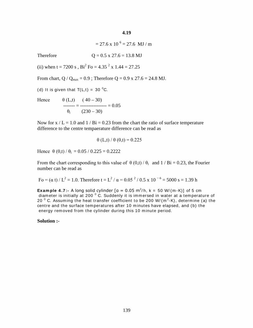
139
4.19
= 27.6 x 10 6 = 27.6 MJ / m Therefore Q = 0.5 x 27.6 = 13.8 MJ (ii) when t = 7200 s , Bi2 Fo = 4.35 2 x 1.44 = 27.25 From chart, Q / Qmax = 0.9 ; Therefore Q = 0.9 x 27.6 = 24.8 MJ. (d) It is given that T(L,t) = 30 0C. Hence θ (L,t) ( 40 – 30) ------- = ---------------- = 0.05 θi (230 – 30) Now for x / L = 1.0 and 1 / Bi = 0.23 from the chart the ratio of surface temperature difference to the centre tempaerature difference can be read as θ (L,t) / θ (0,t) = 0.225 Hence θ (0,t) / θi = 0.05 / 0.225 = 0.2222 From the chart corresponding to this value of θ (0,t) / θi and 1 / Bi = 0.23, the Fourier number can be read as Fo = (α t) / L2 = 1.0. Therefore t = L2 / α = 0.05 2 / 0.5 x 10 − 6 = 5000 s = 1.39 h Example 4.7:- A long solid cylinder [α = 0.05 m2/h, k = 50 W/(m-K)] of 5 cm diameter is initially at 200 0 C. Suddenly it is immersed in water at a temperature of 20 0 C. Assuming the heat transfer coefficient to be 200 W/(m2-K), determine (a) the centre and the surface temperatures after 10 minutes have elapsed, and (b) the energy removed from the cylinder during this 10 minute period. Solution :-
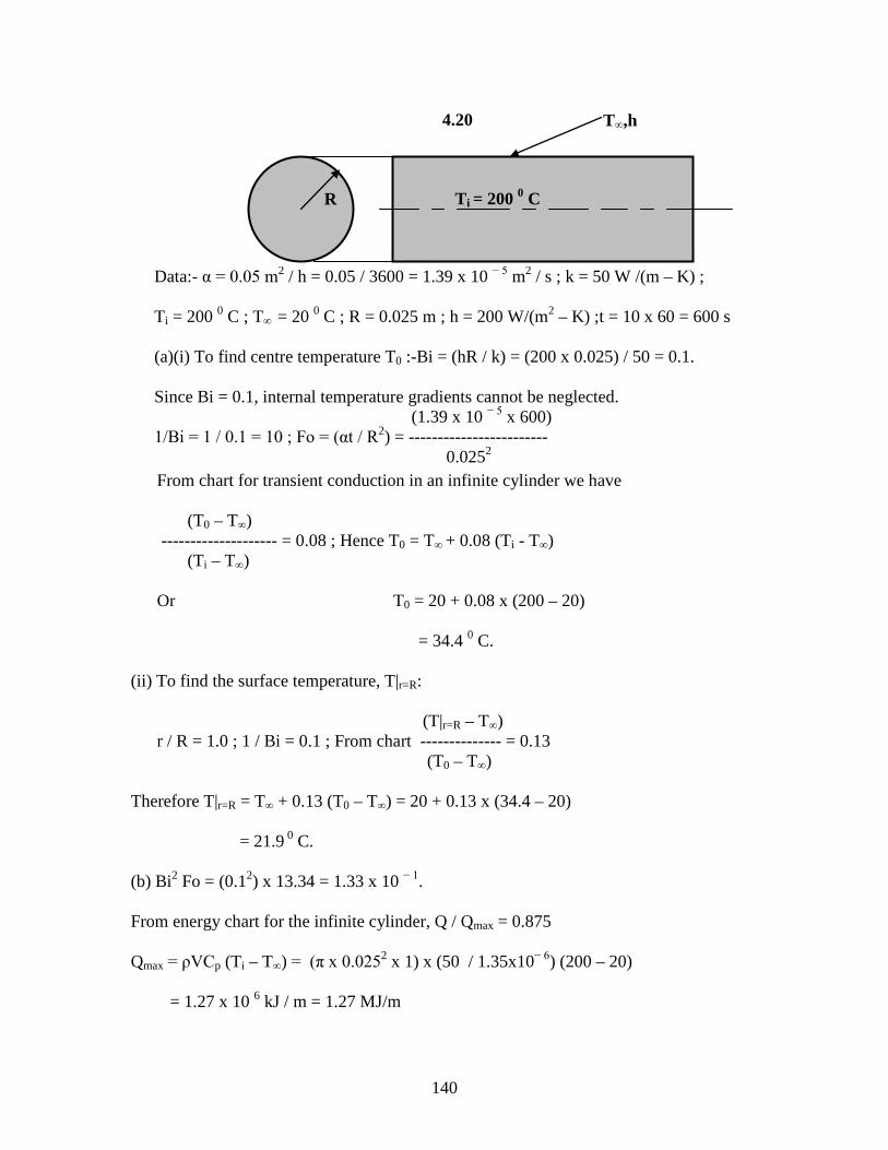
140
From chart for transient conduction in an infinite cylinder we have (T0 – T∞) -------------------- = 0.08 ; Hence T0 = T∞ + 0.08 (Ti - T∞) (Ti – T∞) Or T0 = 20 + 0.08 x (200 – 20) = 34.4 0 C. (ii) To find the surface temperature, T|r=R: (T|r=R – T∞) r / R = 1.0 ; 1 / Bi = 0.1 ; From chart -------------- = 0.13 (T0 – T∞) Therefore T|r=R = T∞ + 0.13 (T0 – T∞) = 20 + 0.13 x (34.4 – 20) = 21.9 0 C. (b) Bi2 Fo = (0.12) x 13.34 = 1.33 x 10 − 1. From energy chart for the infinite cylinder, Q / Qmax = 0.875 Qmax = ρVCp (Ti – T∞) = (π x 0.0252 x 1) x (50 / 1.35x10− 6) (200 – 20) = 1.27 x 10 6 kJ / m = 1.27 MJ/m
R
Data:- α = 0.05 m2 / h = 0.05 / 3600 = 1.39 x 10 − 5 m2 / s ; k = 50 W /(m – K) ; Ti = 200 0 C ; T∞ = 20 0 C ; R = 0.025 m ; h = 200 W/(m2 – K) ;t = 10 x 60 = 600 s (a)(i) To find centre temperature T0 :-Bi = (hR / k) = (200 x 0.025) / 50 = 0.1. Since Bi = 0.1, internal temperature gradients cannot be neglected. (1.39 x 10 − 5 x 600) 1/Bi = 1 / 0.1 = 10 ; Fo = (αt / R2) = ------------------------ 0.0252
Ti = 200 0 C
T∞,h 4.20
141
4.21 Therefore Q = 0.875 x 1.27 = 1.11 MJ / m. Example 4.8:-An orange of 10 cm diameter is initially at a uniform temperature of 30 0C. Suddenly it is placed in a refrigerator in which the air temperature is 2 0 C. If the surface heat transfer coefficient is 50 W/(m2-K), determine the time required for the centre of the orange to reach 10 0 C. Assume for the orange α = 1.4 x 10 ─ 7 m2/s and k = 0.59 W/(m-K). Solution: Orange is assumed to be in the shape of a sphere.
Solution using Tables: - For the given problem we have Bi = 4.24. Therefore from Table 4 – 1 , by interpolation λ1 = 2.4831 and A1 = 1.7362. (T0 – T∞) Therefore -------------- = 0.286 = 1.7362 exp[− λ1
2Fo] (Ti – T∞) Solving for λ1
2Fo we get λ12Fo = 1.804 or Fo = 1.804 / (2.48312) = 0.2925.
Therefore αt / (R2) = 0.2925 (0.2925 x 0.052) Or t = 0.2925 R2 / α = -------------------- = 5223 s = 1 hr 27 mins. 1.4 x 10 − 7
R
R = 0.05 m ; Ti = 30 0 C ; T∞ = 2 0 C ; T0 = 10 0 C ; h = 50 W/(m2 –K);k = 0.59 W/(m – K); α =1.4 x10⁻⁷ m2/s (T0 - T∞) (10 – 2) Now ----------- = θ0 = ---------- = 0.286 (Ti – T∞) (30 – 2 )
1 / Bi = k / hR = 0.59 / (50 x 0.05 ) = 0.24 ; From chart for transient conduction in Sphere we have Fo = (αt / R2) = 0.3. (0.3 x 0.05 2) Therefore t = ------------------ = 5357 s = 1.5 h (1.4 x 10 − 7)

142
4.22 4.3.1. Transient conduction in semi-infinite solids:- A semi-infinite solid is an idealized body that has a single plane surface and extends to infinity in all directions.The transient conduction problems in semi-infinite solids have numerous practical applications in engineering. Consider, for example, temperature transients in a slab of finite but large thickness, initiated by a sudden change in the thermal condition at the boundary surface. In the initial stages, the temperature transients near the boundary surface behave similar to those of semi-infinite medium, because some time is required for the heat to penetrate the slab before the other boundary condition begins to influence the transients.The earth for example, can be considered as a semi-infinite solid in determining the variation of its temperature near its surface We come across basically three possibilities while analyzing the problem of one-dimensional transient conduction in semi-infinite solids.These three problems are as follows: Problem 1:- The solid is initially at a uniform temperature Ti and suddenly at time t>0 The boundary-surface temperature of the solid is changed to and maintained at a uniform temperature T0 which may be greater or less than the initial temperature Ti. Problem 2:- The solid is initially at a uniform temperature Ti and suddenly at time t>0 the boundary surface of the solid is subjected to a uniform heat flux of q0 W/m2. Problem 3:- The solid is initially at a uniform temperature Ti. Suddenly at time t>0 the boundary surface is exposed to an ambience at a uniform temperature T∞ with the surface heat transfer coefficient h. T∞ may be higher or lower than Ti. Solution to Problem 1:- The schematic for problem 1 is shown in Fig. 4.10. The mathematical formulation of the problem to determine the unsteady temperature distribution in an infinite solid T(x,t) is as follows: The governing differential equation is ∂2T / ∂x2 = (1/α) (∂T /∂t) …………………… 4.24(a) The initial condition is at time t = 0, T(x,0) = Ti ………………………………..4.24(b) and the boundary condition is at x = 0, T(0,t) = T0................................................ 4.24(c) It is convenient to solve the above problem in terms of the variable θ(x,t), where θ(x,t) is defined as T(x,t) − T∞ θ(x,t) = ---------------- ………...…………………4.25 Ti − T∞ The governing differential equation in terms of θ(x,t) will be

143
4.23 ∂2θ / ∂x2 = (1/α) (∂θ /∂t) ……………………4.26(a)
The initial condition will be at time t = 0, θ(x,0) = Ti − T∞ …………………….4.26(b) And the boundary condition will be at x = 0, θ(0,t) = T0 − T∞ …………………4.26(c) This problem has been solved analytically and the solution θ(x,t) is represented graphically as θ(x,t) as a function of the dimensionless variable x / [2√(αt)] as shown in Fig. 4.11. In engineering applications, the heat flux at the boundary surface x = 0 is also of interest. The analytical expression for heat flux at the surface is given by k(T0 – Ti) qs(t) = -------------- ……………………..4.27 √(παt) Solution to problem 2:- The schematic for this problem is shown in Fig. 4.12.
x
Initially (t=0), solid at Ti
0
For t > 0, the surface at T0
Fig. 4.10: Semi-infinite solid with specified surface temperature T0 for t > 0
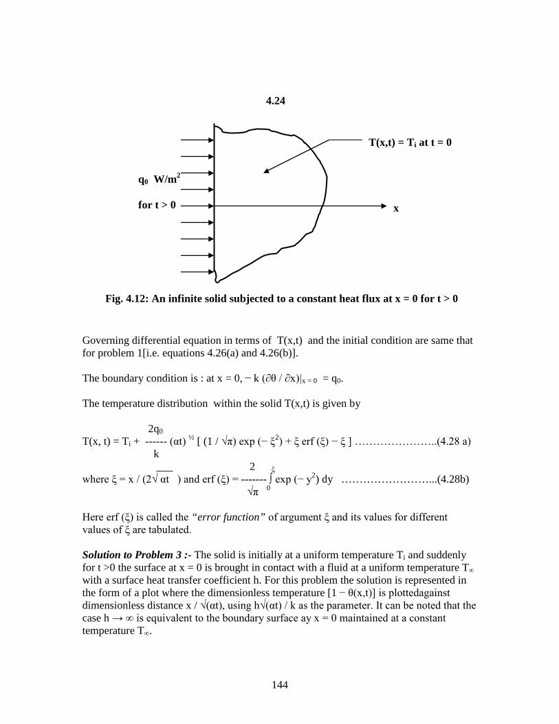
144
Governing differential equation in terms of T(x,t) and the initial condition are same that for problem 1[i.e. equations 4.26(a) and 4.26(b)]. The boundary condition is : at x = 0, − k (∂θ / ∂x)|x = 0 = q0. The temperature distribution within the solid T(x,t) is given by 2q0 T(x, t) = Ti + ------ (αt) ½ [ (1 / √π) exp (− ξ2) + ξ erf (ξ) − ξ ] …………………..(4.28 a) k ___ 2 ξ where ξ = x / (2√ αt ) and erf (ξ) = ------- ∫ exp (− y2) dy ……………………...(4.28b) √π 0 Here erf (ξ) is called the “error function” of argument ξ and its values for different values of ξ are tabulated. Solution to Problem 3 :- The solid is initially at a uniform temperature Ti and suddenly for t >0 the surface at x = 0 is brought in contact with a fluid at a uniform temperature T∞ with a surface heat transfer coefficient h. For this problem the solution is represented in the form of a plot where the dimensionless temperature [1 − θ(x,t)] is plottedagainst dimensionless distance x / √(αt), using h√(αt) / k as the parameter. It can be noted that the case h → ∞ is equivalent to the boundary surface ay x = 0 maintained at a constant temperature T∞.
T(x,t) = Ti at t = 0
q0 W/m2 for t > 0
Fig. 4.12: An infinite solid subjected to a constant heat flux at x = 0 for t > 0
x
4.24
145
4.25 4.3.2. Illustrative examples on Transient Conduction in Semi – Infinite solids Example 4.9:-A thick stainless steel slab [α = 1.6 x 10 ─ 5 m2/s and k = 61 W/(m-K)] is initially at a uniform temperature of 150 0 C. Its surface temperature is suddenly lowered to 20 0 C. By treating this as a one-dimensional transient conduction problem in a semi-infinite medium, determine the temperature at a depth 2 cm from the surface and the heat flux 1 minute after the surface temperature is lowered Solution: Ti = 150 0 C ; T0 = T|x=0 = 20 0 C ; α = 1.6 x 10 − 5 m2 / s ; k = 61 W/(m – K) ; x = 0.02 m ; T = 1 min = 60 s x 0.02 ξ = -------------- = --------------------------------- = 0.323 2 √ (αt) 2 x √ ( 1.6 x 10 − 5 x 60) T(x,t) – T0 From chart, --------------------- = 0.35 Ti – T0 Therefore T(x,t) = T0 + 0.35 (Ti – T0) = 20 + 0.35 x (150 – 20) = 65.5 0 C. k(T0 – Ti) 61 x (20 - 150 qs(t) = --------------------- = ------------------------------ = − 435.5 W / m2
√ (παt) √ (π x 1.6 x 10 − 5 x 60)
Example 4.10:- A semi-infinite slab of copper (α = 1.1 x 10 ─ 4 m2/s and k = 380 W/(m-K) is initially at a uniform temperature of 10 0 C. Suddenly the surface at x = 0 is raised to 100 0C. Calculate the heat flux at the surface 5 minutes after rising of the surface temperature . How long will it take for the temperature at a depth of 5 cm from the surface to reach 90 0 C? Solution: Ti = 10 0 C ; T0 = 100 0 C ; k = 380 W / (m – K) ; α = 1.1 x 10 − 4 m2 / s; t = 300 s ; k(T0 – Ti) 380 x (100 – 10) qs(t) = ------------------- = -------------------------------- = 11012 W / m2 = 11.012 kW/m2
√ (παt) √ (π x 1.1 x 10 − 4 x 300) T(x,t) – T0 90 – 100 θ(x,t) = ------------------ = --------------------- = 0.11 . From chart ξ = 0.1 Ti – T0 10 – 100

146
4.26 x x2 0.05 2
ξ = -------------- or t = ------------------- = ------------------------------ 2√ (αt) 4 α ξ 2 4 x 1.1 x 10 − 4 x (0.1) 2 = 586 s = 9.46 min Example 4.11:-A thick bronze [α = 0.86 x 10 ─ 5 m2/s and k = 26 W/(m-K)] is initially at 250 0 C. Suddenly the surface is exposed to a coolant at 25 0 C. If the surface heat transfer coefficient is 150 W/(m2-K), determine the temperature 5 cm from the surface 10 minutes after the exposure. Solution: Ti = 250 0 C; T∞ = 25 0 C; h = 150 W/(m2 – K) ; k = 26 W /(m – K) ; α = 0.86 x 10 −5 m2/s t = 600 s ; x = 0.05 m ; x 0.05 ξ = ---------------- = ------------------------------------ = 0.35 2 √(α t) 2 x √ ( 0.86 x 10 − 5 x 600) ____ __________________ h √(α t) 150 x √ [ 0.86 x 10 − 5 x 600] -------------- = -------------------------------------- = 0.414 K 26 [T(x,t) – T∞] Therefore from chart 1 − ------------------------ = 0.15 (Ti – T∞) Solving for T(x,t) we have T(x,t) = T∞ + (1 – 0.15)(Ti – T∞) = 25 + 0.85 x (250 – 25 ) = 216.25 0 C. Example 4.12:- A thick wood [α = 0.82 x 10 ─ 7 m2/s and k = 0.15 W/(m-K)] is initially at 20 0 C. The wood may ignite at 400 0 C. Suddenly the surface of the wood is exposed to gases at 500 0 C. If the surface heat transfer coefficient is 45 W/(m2- K), how long will it take for the surface of the wood to reach 400 0 C ? Solution: Ti
= 20 0 C ; T∞ = 500 0C ; h = 45 W /(m 2 – K) ; k = 0.15 W /(m – K) ; α = 0.82 x 10 − 7 m2 / s.

147
4.27 ____ _______________ h √ (α t) 45 x √ (0.82 x 10 − 7 x t) ---------- = ------------------------------- = 0.086 √t k 0.15 ____ T(x,t) – T∞ (400 – 500) x / 2√( α t) = 0. Also 1 − -------------------- = 1 − ------------------- = 0.9799 Ti – T∞ (20 – 5000) ___ Hence from chart h √(α t) / k = 2.75. _ Therefore 0.086 √ t = 2.75 or t = 1023 s = 17 min.

148
Chapter 5
Basic Concepts of Convective Heat Transfer
5.1. Definition of Convective Heat Transfer:- When a fluid flows over a body or inside a channel and if the temperatures of the fluid and the solid surface are different, heat transfer will take place between the solid surface and the fluid due to the macroscopic motion of the fluid relative to the surface. This mechanism of heat transfer is called as “convective heat transfer”.If the fluid motion is due to an external force (by using a pump or a compressor) the heat transfer is referred to as “forced convection”. If the fluid motion is due to a force generated in the fluid due to buoyancy effects resulting from density difference (density difference may be caused due to temperature difference in the fluid) then the mechanism of heat transfer is called as “natural or free convection”.For example, a hot plate suspended vertically in quiescent air causes a motion of air layer adjacent to the plate surface because the temperature gradient in the air gives rise to a density gradient which in turn sets up the air motion. 5.2. Heat Transfer Coefficient:- In engineering application, to simplify the heat transfer calculations between a hot surface say at temperature Tw and a cold fluid flowing over it at a bulk temperature T∞ as shown in Fig. 5.1 a term called “heat transfer coefficient,h” is defined by the equation
q = h(Tw – T∞)………………………………………………..5.1(a)
where q is the heat flux (expressed in W / m2) from the surface to the flowing fluid. Alternatively if the surface temperature is lower than the flowing fluid then the heat transfer takes place from the hot fluid to the cold surface and the heat flux is given by
q = h(T∞ – Tw)………………………………………………..5.1(b)
The heat flux in this case takes place from the fluid to the cold surface.If in equations 5.1(a) and 5.1(b) the heat flux is expressed in W / m2, then the units of heat transfer coefficient will be W /(m 2 – K) or W / (m 2 – 0 C). The heat transfer coefficient is found to vary with (i) the geometry of the body, (ii) the type of flow (laminar or turbulent), (iii) the transport properties of the fluid (density, viscosity and thermal conductivity),(iv) the average temperature, (v) the position along the surface of the body, and (vi) whether the heat transfer is by forced convection or free convection. For convection problems involving simple geometries like flow over a flat plate or flow inside a circular tube, the heat transfer coefficient can be

149
determined analytically. But for flow over complex configurations, experimental / numerical approach is used to determine h.There is a wide difference in the range of values of h for various applications.Typical values of heat transfer coefficients encountered in some applications are given in Table 5.1. Table 5.1: Typical Values of heat transfer coefficients Type of flow h [W /(m2 – K) ] Free convection air 5 – 15 -----do --------- oil 25 – 60 -----do--------- water 400 –800 Forced Convection air 15 –300 -------do------------ oil 50 –1700 -------do----------- water 300 – 12000 Boiling water 3000 – 55000 Condensing steam 5500 – 120000
u∞, T∞ T∞
Tw
Fluid Temperature Profile
x
Fig. 5.1: Temperature distribution of the fluid at any x for Tw > T∞

150
5.3. Basic concepts for flow over a body:- When a fluid flows over a body, the velocity and temperature distribution at the vicinity of the surface of the body strongly influence the heat transfer by convection.By introducing the concept of boundary layers (velocity boundary layer and thermal boundary layer) the analysis of convective heat transfer can be simplified. 5.3.1.Velocity Boundary Layer:- Consider the flow of a fluid over a flat plate as shown in Fig. 5.2. The fluid just before it approaches the leading edge of the plate has a velocity u∞ which is parallel to the plate surface.As the fluid moves in x-direction along the plate,
those fluid particles that makes contact with the plate surface will have the same velocity as that of the plate. Therefore if the plate is stationary, then the fluid layer sticking to the plate surface will have zero velocity.But far away from the plate (y = ∞) the fluid will have the velocity u∞.Therefore starting from the plate surface (y = 0) there will be retardation of the fluid in x-direction component of velocity u(x,y).This retardation effect is reduced as we move away from the plate surface.At distances sufficiently long from the plate(y = ∞) the retardation effect is completely reduced: i.e. u → u∞ as y → ∞. This means that there is a region surrounding the plate surface where the fluid velocity changes from zero at the surface to the velocity u∞ at the outer edge of the region. This region is called the velocity boundary layer. The variation of the x-component of velocity u(x,y) with respect to y at a particular location along the plate is shown in Fig. 5.2.The distance measured normal to the surface from the plate surface to the point at which the fluid attains 99% of u∞ is called “velocity boundary layer thickness” and denoted by δ(x) Thus for flow over a flat plate, the flow field can be divided into two distinct regions, namely, (i) the boundary layer region in which the axial component of velocity u(x,y) varies rapidly with y with the result the velocity gradient (∂u /∂y) and hence the shear
x
y
Laminar Region Transition Turbulent Region
Fig. 5.2: Velocity boundary layer for flow over a flat plate
u∞
u(x, y)
xcr
u(x, y)
151
stress are very large and (ii) the potential flow region which is outside the boundary layer region, where the velocity gradients and shear stresses are negligible. The flow in the boundary layer, starting from the leading edge of the plate will be initially laminar in which the fluid particles move along a stream line in an orderly manner. In the laminar region the retardation effect is due to the viscosity of the fluid and therefore the shear stress can be evaluated using Newton’s law of viscocity.The laminar flow continues along the plate until a critical distance ‘xcr’ is reached. After this the small disturbances in the flow begin to grow and fluid fluctuations begin to develop. This characterizes the end of the laminar flow region and the beginning of transition from laminar to turbulent boundary layer. A dimensionless parameter called Reynolds number is used to characterize the flow as laminar or turbulent. For flow over a flat plate the Reynolds number is defined as u∞ x Rex = ---------- …………………………….5.2 ν where u∞ = free-stream velocity of the fluid, x = distance from the leading edge of the plate and ν = kinematic viscosity of the fluid. For flow over a flat plate it has been found that the transition from laminar flow to turbulent flow takes place when the Reynolds number is ≈ 5 x 10 5.This number is called as the critical Reynolds number Recr for flow over a flat plate.Therefore u∞ xcr Recr = -------------- = 5 x 10 5 ……………….5.3 ν The critical Reynolds number is strongly dependent on the surface roughness and the turbulence level of the free stream fluid. For example, with very large disturbances in the free stream, the transition from laminar flow to turbulent flow may begin at Rex as low as 1 x 10 5 and for flows which are free from disturbances and if the plate surface is smooth transition may not take place until a Reynolds number of 1 x 10 6 is reached.But it has been found that for flow over a flat plate the boundary layer is always turbulent for Rex ≥ 4 x 10 6.In the turbulent boundary layer next to the wall there is a very thin layer called “the viscous sub-layer”, where the flow retains its viscous flow character. Next to the viscous sub-layer is a region called “buffer layer” in which the effect of fluid viscosity is of the same order of magnitude as that of turbulence and the mean velocity rapidly increases with the distance from the plate surface.Next to the buffer layer is “the turbulent layer” in which there is large scale turbulence and the velocity changes relatively little with distance. 5.3.2. Drag coefficient and Drag force:- If the velocity distribution u(x,y) in the boundary layer at any ‘x’ is known then the viscous shear stress at the wall can be determined using Newton’s law of viscosity. Thus if τw(x) is the wall-shear stress at any location x then
152
τw(x) = μ(∂u / ∂y)y = 0 ………………….5.4 where μ is the absolute viscosity of the fluid.The drag coefficient is dimensionless wall shear stress. Therefore the local drag coefficient, Cx at any ‘x’ is defined as τw(x) Cx = ------------- ……………………….5.5 (1/2) ρu∞
2 Substituting for τw(x) in the above equation from Eq. 5.4 and simplifying we get 2ν (∂u / ∂y)y = 0 Cx = ---------------------- ……………….5.6 u∞
2 Therefore if the velocity profile u(x,y) at any x is known then the local drag coefficient Cx at that location can be determined from Eq. 5.6.The average value of Cx for a total length L of the plate can be determined from the equation L Cav = (1/L) ∫Cx dx ……………………5.7 0 Substituting for Cx from Eq. 5.5 we have L ∫ τw(x)dx Cav = ------------------------ L (1/2) ρu∞
2 _ τw Or Cav = -------------------- ……………….5.8 (1/2) ρu∞
2 _ Where τw is the average wall-shear stress for total length L of the plate. The total drag force experienced by the fluid due to the presence of the plate can be written as _ FD = As τw …………………………….5.9 Where As is the total area of contact between the fluid and the plate. If ‘W’ is the width of the plate then As = LW if the flow is taking place on one side of the plate and As = 2LW if the flow is on both sides of the plate. 5.3.3.Thermal boundary layer:- Similar to the velocity boundary layer one can visualize the development of a thermal boundary layer when a fluid flows over a flat
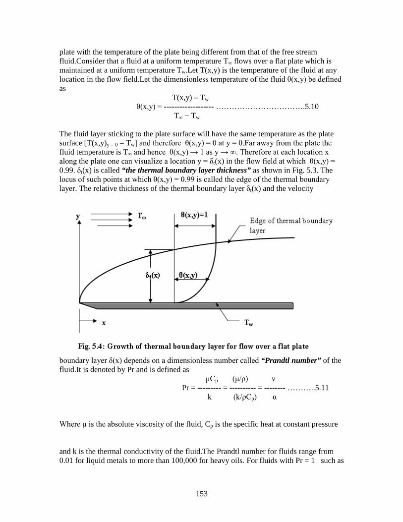
153
plate with the temperature of the plate being different from that of the free stream fluid.Consider that a fluid at a uniform temperature T∞ flows over a flat plate which is maintained at a uniform temperature Tw.Let T(x,y) is the temperature of the fluid at any location in the flow field.Let the dimensionless temperature of the fluid θ(x,y) be defined as T(x,y) – Tw θ(x,y) = ------------------- …………………………….5.10 T∞ − Tw The fluid layer sticking to the plate surface will have the same temperature as the plate surface [T(x,y)y = 0 = Tw] and therefore θ(x,y) = 0 at y = 0.Far away from the plate the fluid temperature is T∞ and hence θ(x,y) → 1 as y → ∞. Therefore at each location x along the plate one can visualize a location y = δt(x) in the flow field at which θ(x,y) = 0.99. δt(x) is called “the thermal boundary layer thickness” as shown in Fig. 5.3. The locus of such points at which θ(x,y) = 0.99 is called the edge of the thermal boundary layer. The relative thickness of the thermal boundary layer δt(x) and the velocity
boundary layer δ(x) depends on a dimensionless number called “Prandtl number” of the fluid.It is denoted by Pr and is defined as μCp (μ/ρ) ν Pr = --------- = ---------- = -------- ………..5.11 k (k/ρCp) α Where μ is the absolute viscosity of the fluid, Cp is the specific heat at constant pressure
and k is the thermal conductivity of the fluid.The Prandtl number for fluids range from 0.01 for liquid metals to more than 100,000 for heavy oils. For fluids with Pr = 1 such as

154
gases δt(x) = δ(x), for fluids with Pr << 1such as liquid metals δt(x) >> δ(x) and for fluids with Pr >> 1, like oils δt(x) << δ(x). 5.3.4. General expression for heat transfer coefficient:- Let us assume that Tw > T∞.Then heat is transferred from the plate to the fluid flowing over the plate.Therefore at any ‘x’ the heat flux is given by q = − k (∂T /∂y)y=0 ………………………..5.12(a) In terms of the local heat transfer coefficient hx, the heat flux can also be written as q = hx (Tw − T∞) …………………………..5.12(b) From equations 5.12(a) and 5.12(b) it follows that − k (∂T /∂y)y=0 hx = ------------------ ………………………5.13 (Tw − T∞) From equation 5.10 we have (∂T /∂y)y=0 = [T∞ − Tw] (∂θ /∂y)y=0. Substituting this expression in Eq.5.13 and simplifying we get the general expression for hx as hx = k (∂θ /∂y)y=0 ………………………….5.14 The same expression for hx could be obtained even when Tw < T∞. Equation 5.14 can be used to determine the local heat transfer coefficient for flow over a flat plate if the dimensionless temperature profile θ(x,y) is known. Average heat transfer coefficient:- For a total length L of the plate the average heat transfer coefficient is given by L hav = (1 /L) ∫hxdx ………………………….5.15 0
Substituting for hx from Eq. 5.14 we get L hav = (1 /L) ∫ k (∂θ /∂y)y=0 dx ………………….5.15 0
Since (∂θ /∂y)y=0 at any x depends on whether the flow at that section is laminar or turbulent the expression for hav can be written as xcr L hav = (1 /L) { ∫ k [(∂θ /∂y)y=0]laminar dx + ∫ k [(∂θ /∂y)y=0]turbulent dx }……5.16 0 xcr

155
5.3.5. Illustrative examples on flow over a flat plate: Example 5.1:- Assuming the transition from laminar to turbulent flow takes place at a Reynolds number of 5 x 10 5, determine the distance from the leading edge of a flat plate at which transition occurs for the flow of each of the following fluids with a velocity of 2 crm/s at 40 0 C.(i) Air at atmospheric pressure;(ii)Hydrogen at atmospheric pressure;(iii) water;(iv) Engine oil;(v) mercury.Comment on the type of flow for the 5 fluids if the total length of the plate is 1 m. Solution: Data:- Recr = 5 x 10 5; u∞ = 2 m/s ; T∞ = 40 0 C (i)Air at atmospheric pressure :- At 40 0 C, ν = 17 x 10 − 6 m2/s. u∞ xcr Recr ν 5 x 10 5 x 17 x 10 − 6
Recr = ----------- or xcr = -------------------- = ---------------------------- = 4.25 m. ν u∞ 2 (ii) Hydrogen :- For hydrogen at 40 0 C, ν = 117.9 x 10 − 6 m2/s. 5 x 10 5 x 117.9 x 10 − 6
Therefore xcr = ------------------------------- = 29.5 m 2 (iii) Water :- For water at 40 0 C, ν = 0.658 x 10 − 6 m2/s. 5 x 10 5 x 0.658 x 10 − 6
Therefore xcr = ------------------------------- = 0.1645 m 2 (iv) Engine oil :- For engine oil at 40 0 C, ν = 0.24 x 10 − 3 m2/s. 5 x 10 5 x 0.24 x 10 − 3
Therefore xcr = ------------------------------- = 60 m 2 (v) Mercury :- For mercury at 40 0 C, ν = 0.107 x 10 − 6 m2/s. 5 x 10 5 x 0.107 x 10 − 6
Therefore xcr = ------------------------------- = 0.027 m 2 Comments on the type of flow

156
Sl.No Type of fluid xcr xcr vs L Type of Flow 1 Air 4.25 xcr > L Flow is Laminar for entire length 2 Hydrogen 29.5 xcr>> L Flow is laminar for entire length 3 Water 0.1645 xcr < L Flow is partly Laminar & Partly Turbulent 4 Engine oil 60 xcr >> L Flow is laminar for entire length 5 Mercury 0.027 xcr << L Flow is turbulent for almost entire length Example 5.2:- An approximate expression for the velocity profile u(x,y) for laminar boundary layer flow along a flat plate is given by u(x, y)/ u∞ =2[y / δ(x)] − 2[y / δ(x)] 3+ [y / δ(x)] 4 where δ(x) is the velocity boundary layer thickness given by the expression δ(x) / x = 5.83 / (Rex)1/2
(a) Develop an expression for the local drag coefficient. (b) Develop an expression for the average drag coefficient for a length L of the plate. (c) Determine the drag force acting on the plate 2 m x 2 m for flow of air with a free
stream velocity of 4 m /s and a temperature of 80 0C. Solution:- (a) The velocity profile u(x,y) is given as
u(x, y) = u∞ {2[y / δ(x)] − 2[y / δ(x)] 3+ [y / δ(x)] 4 } Therefore (∂u / ∂y)y=0 = 2u∞ / δ(x)
τw(x) = μ (∂u / ∂y)y=0 = (2 μu∞) / δ(x) (2 μu∞) Rex (2 μu∞) [(u∞x) / ν]1/2 = ----------------- = ------------------------ = 0.343 (μu∞) [u∞ /(x ν)]1/2 ….(1 ) 5.83 x 5.83 x

157
The local drag coefficient at any x is given by τw(x) 0.343 (μu∞) [u∞ /(x ν)]1/2 Cx = ----------------- = ------------------------------------------- (1/2) ρu∞
2 (1/2) ρu∞2
0.686 0.686 = ---------------------- = ----------------- {(u∞x) / ν}1/2 (Rex) ½ (b) The average drag coefficient is given by L L Cav = (1/L) ∫ Cx dx = (1/L) ∫ 0.686 (Rex) − ½ dx
0 0
{ 0.686 (u∞/ν) − ½} L = ----------------------- ∫ x − ½ dx L 0 Or 2 x 0.686 1.372 Cav = --------------- = ------------------ (u∞L / ν) ½ (ReL) ½ (c) At 80 0 C for air ν = 20.76 x 10 − 6 m2 / s ; ρ = 1.00 kg / m 3 u∞L 4 x 2 ReL = ----------------- = ------------------- = 3.793 x 10 5
ν 21.09 x 10 − 6 1.372 1.372 Average drag coefficient = Cav = ------------------- = ------------------------ = 2.228 x 10 − 3
ReL0.5 (3.793 x 10 5)0.5
Drag force assuming that the flow takes place on one side of the plate is given by
_ FD = τw LW = (1/2)ρ u∞
2 Cav LW for flow over one side of the plate = (1/2) x 1.00 x 42 x 2.2228 x 10 − 3 x 2 x 2 =0.071 N

158
Example 5.3:- An approximate expression for temperature profile θ(x,y) in the thermal boundary layer region is given by θ(x,y) = 2y / δt −[y / δt]2 where the thermal boundary layer thickness δt is given by 5.5 δt / x = ----------------- ; Rex is the Reynolds number based on ‘x’ and Rex
0.5Pr 1/3 Pr is the Prandtl number of the fluid. Develop an expression for (i) the local heat transfer coefficient hx and (ii) the average heat transfer coefficient for total length L of the plate. Solution: (i) The local heat transfer coefficient hx is given by hx = k (∂θ / ∂y)|y = 0.
Now θ(x,y) = 2y / δt −[y / δt]2 2 Rex
0.5Pr 1/3 Hence (∂θ / ∂y)|y = 0. = 2 / δt = --------------------- 5.5.x 2 k Rex
0.5Pr 1/3 Or hx = ------------------------ = 0.364 (k / x) Rex
0.5 Pr 1/3
5.5.x Or hx x ----- = 0.364 Rex
0.5 Pr 1/3
K hx x ---- is a dimensionless number involving local heat transfer coefficient and is called k “local Nusselt number”. (ii) The average heat transfer coefficient for a total length L of the plate is given by L hav = (1 / L) ∫hx dx = (1 / L) ∫ 0.364 (k / x) Rex
0.5 Pr1/3 dx 0 L Or = (1 / L) 0.364 Pr1/3 k (U∞ / ν)0.5 ∫ x − 0.5 dx 0 L 0.5
= (1 / L) ----------- 0.364 Pr1/3 k (U∞ / ν)0.5 0.5 = 0.728 (k / L) (U∞L / ν) 0.5 Pr 1/3
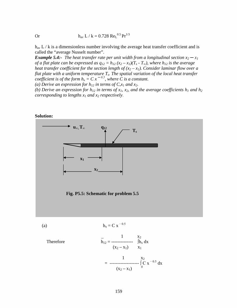
159
Or hav L / k = 0.728 ReL
0.5 Pr1/3 hav L / k is a dimensionless number involving the average heat transfer coefficient and is called the “average Nusselt number”. Example 5.4:- The heat transfer rate per unit width from a longitudinal section x2 ─ x1 of a flat plate can be expressed as q12 = h12 (x2 – x1)(Ts - T∞), where h12 is the average heat transfer coefficient for the section length of (x2 – x1). Consider laminar flow over a flat plate with a uniform temperature Ts. The spatial variation of the local heat transfer coefficient is of the form hx = C x ─ 0.5, where C is a constant. (a) Derive an expression for h12 in terms of C,x1 and x2. (b) Derive an expression for h12 in terms of x1, x2, and the average coefficients h1 and h2 corresponding to lengths x1 and x2 respectively. Solution:
(a) hx = C x − 0.5 _ 1 x2 Therefore h12 = -------------- ∫hx dx (x2 – x1) x1 1 x2 = ------------------- ∫ C x − 0.5 dx (x2 – x1) 0
x1
x2
u∞, T∞ Ts
Fig. P5.5: Schematic for problem 5.5
q12

160
2C = ------------------ [ x2
0.5 – x1 0.5]
(x2 – x1) _ x1
(b) h1 = (1/x1) ∫C x − 0.5 dx 0 = 2C / √ x1 _ ___ Similarly h2 = 2C / √ x2 x1 _ 1 x2 x1
Therefore Since ∫ hxdx = x1h1, h12 = -------------- [ ∫ hxdx - ∫ hxdx ] 0 ( x2 – x1) 0 0
_ _ _ h2x2 - h1x1 h12 = ----------------- x2 – x1
5.4. Basic Concepts For Flow Through Ducts :- The basic concepts developed on the development of velocity and thermal boundary layers for flow over surfaces are also applicable to flows at the entrance region of the ducts. 5.4.1.Velocity Boundary Layer:- Consider the flow inside a circular tube as shown in Fig.5.4. Lat uo be the uniform velocity with which the fluid approaches the tube. As the fluid enters the tube, a “velocity boundary layer” starts to develop along the wall-surface. The velocity of the fluid layer sticking to the tube-surface will have zero velocity and the fluid layer slightly away from the wall is retarded. As a result the velocity in the central portion of the tube increases to satisfy the continuity equation (law of conservation of mass).The thickness of the velocity boundary layer δ(z) continuously grows along the tube-surface until it fills the entire tube. The region from the tube inlet up to little beyond the hypothetical location where the boundary layer reaches the tube centre is called “hydrodynamic entrance region or hydrodynamically developing region” and the
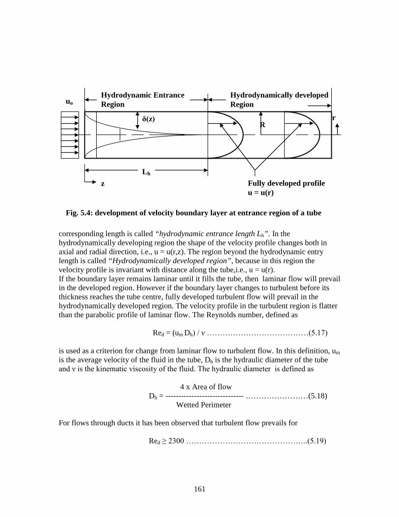
161
corresponding length is called “hydrodynamic entrance length Lh”. In the hydrodynamically developing region the shape of the velocity profile changes both in axial and radial direction, i.e., u = u(r,z). The region beyond the hydrodynamic entry length is called “Hydrodynamically developed region”, because in this region the velocity profile is invariant with distance along the tube,i.e., u = u(r). If the boundary layer remains laminar until it fills the tube, then laminar flow will prevail in the developed region. However if the boundary layer changes to turbulent before its thickness reaches the tube centre, fully developed turbulent flow will prevail in the hydrodynamically developed region. The velocity profile in the turbulent region is flatter than the parabolic profile of laminar flow. The Reynolds number, defined as Red = (um Dh) / ν …………………………………(5.17) is used as a criterion for change from laminar flow to turbulent flow. In this definition, um is the average velocity of the fluid in the tube, Dh is the hydraulic diameter of the tube and ν is the kinematic viscosity of the fluid. The hydraulic diameter is defined as 4 x Area of flow Dh = ------------------------------ ……………………(5.18) Wetted Perimeter For flows through ducts it has been observed that turbulent flow prevails for Red ≥ 2300 ………………………………………..(5.19)
uo
Lh
z
Hydrodynamic Entrance Region
Hydrodynamically developed Region
Fully developed profile u = u(r)
δ(z) R
Fig. 5.4: development of velocity boundary layer at entrance region of a tube
r

162
But this critical value is strongly dependent on the surface roughness, the inlet conditions and the fluctuations in the flow. In general, transition may occur in the range 2000 < Red < 4000. It is a common practice to assume a value of 2300 fro transition from laminar flow to turbulent flow. 5.4.2. Friction Factor and Pressure Drop Relations For Hydrodynamically Developed Laminar Flow In engineering applications, the pressure gradient (dp / dz) associated with the flow is a quantity of interest, because this decides the pumping power required to overcome thr frictional losses in the pipe of a given length. Consider a differential length dz of the tube at a distance z from the entrance and let this length be in the fully developed region. The various forces acting on the fluid element in the direction of flow are shown in Fig.5.5. Resultant force in the direction of motion = F = (pA)z –(pA)z+dz – τw Sdz where S is the perimeter of the duct. Using Taylor’s series expansion and neglecting higher order terms we can write (pA)z+dz = (pA)z + d/dz(pA) dz Therefore F = d/dz(pA) dz − τw Sdz Rate of change of momentum in the direction of flow = 0 because the velocity u does not vary with respect to z in the fully developed region. Hence d/dz(pA) dz − τw Sdz = 0 For duct of uniform cross section A is constant. Therefore the above equation reduces to dp/dz = − τw S /A ……………………………….(5.20) For laminar flow τw = − μ (du / dr)|wall. Hence Eq. (5.20) reduces to dp μS ------ = -------- (du/dr)|wall ……………………….(5.21) dz A Eq.(5.21) is not practical for the determination of (dp/dz), because it requires the evaluation f the velocity gradient at the wall. Hence for engineering applications a parameter called “friction factor, f ” is defined as follows:

163
(dp/dz) Dh f = − ------------------- ………………………….(5.22a) ½ (ρum
2) Substituting for (dp/dz) from Eq. (5.21) we have (μS/A) (du/dr)|wall Dh f = − ---------------------------- …………………..(5.22b) ½ (ρum
2) For a circular tube S = πDi, and A = πDi
2 / 4. Hence Dh = Di
Hence for a circular tube Eq. (5.22b) reduces to 8μ f = − ------- (du/dr)|wall …………………………(5.22c) (ρum
2) Also from Eq. (5.22a) we have (½ ) (ρum
2) f dp = − ----------------- dz Dh Integrating the above equation over a total length L of the tube we have
p2 (½ ) (ρum
2) f L ∫dp = − ------------------- ∫dz p1 Dh 0 or pressure drop = Δp = (p1 – p2) = ( ½ ) (L/Dh) f ρum
2 …………………………(5.23) . Pumping power is given by P = V Δp ………………………………………...(5.24) . where V = volume flow rate of the fluid. 5.4.3. Thermal Boundary Layer: In the case of temperature distribution in flow inside a tube, it is more difficult to visualize the development of thermal boundary layer and the existence of thermally developed region. However under certain heating or cooling conditions such as constant wall-heat flux or constant wall-temperature it is possible to have thermally developed region. Consider a laminar flow inside a circular tube subjected to uniform heat flux at the wall. Let ‘r’ and ‘z’ be the radial and axial coordinates respectively and T(r,z) be the local fluid temperature. A dimensionless temperature θ(r,z) is defined as T(r,z) – Tw(z) θ(r,z) = ------------------- ………………………………..(5.25a) Tm(z) – Tw(z)
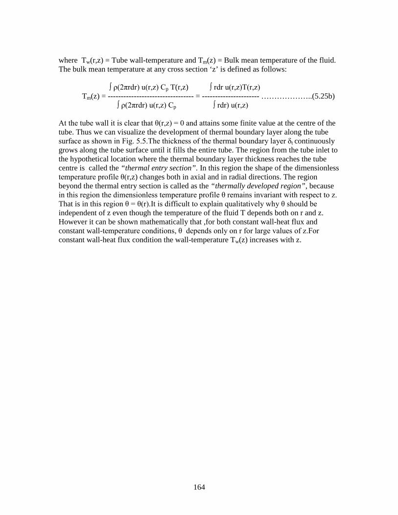
164
where Tw(r,z) = Tube wall-temperature and Tm(z) = Bulk mean temperature of the fluid. The bulk mean temperature at any cross section ‘z’ is defined as follows: ∫ ρ(2πrdr) u(r,z) Cp T(r,z) ∫ rdr u(r,z)T(r,z) Tm(z) = --------------------------------- = ---------------------- ………………..(5.25b) ∫ ρ(2πrdr) u(r,z) Cp ∫ rdr) u(r,z) At the tube wall it is clear that θ(r,z) = 0 and attains some finite value at the centre of the tube. Thus we can visualize the development of thermal boundary layer along the tube surface as shown in Fig. 5.5.The thickness of the thermal boundary layer δt continuously grows along the tube surface until it fills the entire tube. The region from the tube inlet to the hypothetical location where the thermal boundary layer thickness reaches the tube centre is called the “thermal entry section”. In this region the shape of the dimensionless temperature profile θ(r,z) changes both in axial and in radial directions. The region beyond the thermal entry section is called as the “thermally developed region”, because in this region the dimensionless temperature profile θ remains invariant with respect to z. That is in this region θ = θ(r).It is difficult to explain qualitatively why θ should be independent of z even though the temperature of the fluid T depends both on r and z. However it can be shown mathematically that ,for both constant wall-heat flux and constant wall-temperature conditions, θ depends only on r for large values of z.For constant wall-heat flux condition the wall-temperature Tw(z) increases with z.
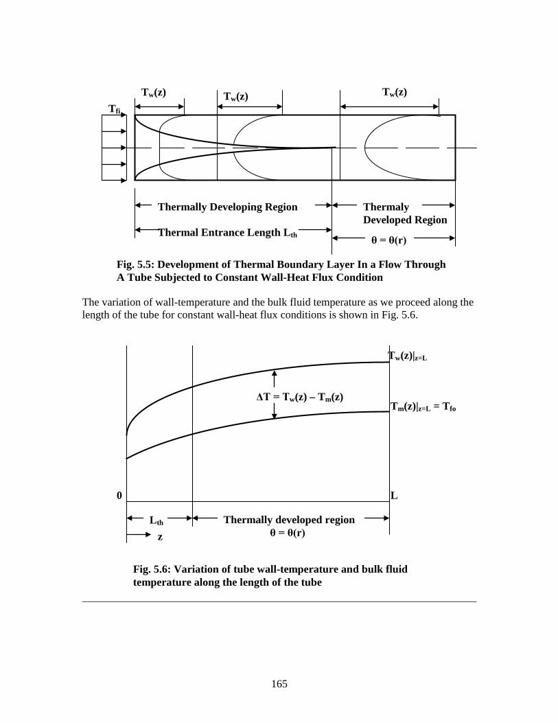
165
The variation of wall-temperature and the bulk fluid temperature as we proceed along the length of the tube for constant wall-heat flux conditions is shown in Fig. 5.6.
Lth
z
ΔT = Tw(z) – Tm(z)
Fig. 5.6: Variation of tube wall-temperature and bulk fluid temperature along the length of the tube
Tw(z)|z=L Tm(z)|z=L = Tfo
Thermally developed region θ = θ(r)
0 L
Tfi
Tw(z) Tw(z)
Tw(z)
Thermally Developing Region Thermal Entrance Length Lth
Thermaly Developed Region
θ = θ(r)
Fig. 5.5: Development of Thermal Boundary Layer In a Flow Through A Tube Subjected to Constant Wall-Heat Flux Condition

166
It can be shown that for constant wall-heat flux condition the temperature difference ΔT between the tube wall and the bulk fluid remains constant along the length of the tube. The growth of the thermal boundary layer for constant wall-temperature conditions is similar to that for constant wall-heat flux condition except that the wall temperature does not vary with respect to z. Therefore the temperature profile T(r,z) becomes flatter and flatter as shown in Fig. 5.7 as we proceed along the length of the tube and eventually the fluid temperature becomes equal to the wall temperature. Since the
wall-temperature remains constant and the bulk fluid temperature varies along the length
Tfi Tw
Tw Tw Tw
z Thermally developing region Thermal entrance length Lth
Thermally developed region
Fig.5.7: Growth of thermal boundary layer for flow through a tube with constant wall-temperature

167
the temperature difference between the tube wall and the bulk fluid varies along the length of the tube as shown in Fig. 5.8. 5.4.4. Mean Temperature Difference, ΔTm: If Q is the total heat transfer rate between the fluid and the tube surface , As is the area of contact between the fluid and the surface, hm is the average heat transfer coefficient for the total length of the tube then we can write Q = hm As ΔTm …………………………….(5.26) Where ΔTm = mean temperature difference between the tube wall and the bulk fluid. For a tube with constant wall-heat flux condition, since the temperature difference between the fluid and the tube surface remains constant along the length of the tube it follows that ΔTm = [Tw(z)|z=0 − Tfi] = [Tw(z)|z=L − Tfo] …………………(5.27a) For a tube with constant wall-temperature condition the mean temperature difference is given by ΔTi – ΔTo ΔTm = ----------------------- ………………………………….(5.27b) ln (ΔTi / ΔTo) 5.4.5. General expression for heat transfer coefficient : Let the fluid be heated as it flows through the tube. Then at any z the heat flux from the tube surface to the fluid is given by Fourier’s law as
z
Tw
Tfi
Tfo
L 0
ΔTi
ΔTo
Fig. 5.8: Variation of bulk fluid temperature along the length of the tube for tube with constant wall-temperature

168
qw(z) = k (∂T / ∂r)|wall ……………………(5.28) [Note that when the fluid is heated Tw> Tm so that (∂T / ∂r)|wall will be positive). If hz is the heat transfer coefficient then qw(z) = hz [Tw(z) – Tm(z) …………….(5.29) Therefore from Eq. (5.28) and (5.29) we have k (∂T / ∂r)|wall hz = ------------------- ……………………(5.30) [Tw(z) – Tm(z)] [T(r,z) – Tw(z)] Now θ(r,z) = -------------------- [Tm(z) – Tw(z)] Therefore (∂T / ∂r)|wall = [Tm(z) – Tw(z)] (∂θ / ∂r)|wall
5.21 Substituting this expression in Eq. (5.30) and simplifying we get hz = − k (∂θ / ∂r)|wall ………………………….(5.31) In the thermally developed region θ depends only on r. Hence hz = − k (dθ / dr)|wall …………………………(5.32) Since (dθ / dr)|wall is independent of z it follows that the heat transfer coefficient hz is independent of z. This is true both for constant wall-temperature and constant wall-heat flux conditions. 5.4.6.Illustrative Examples on Flow Through Ducts: Example 5.5:- The velocity profile for hydrodynamically developed laminar flow inside a circular tube of radius R is given by u(r) = 2um[ 1 – (r/R)2] where um is the average velocity of the fluid in the tube.Develop an expression for the friction factor f and express it in terms of the Reynolds number Red where Red is defined as Red = (umD) / ν. Solution: u(r) = 2um[ 1 – (r/R)2] Therefore (du / dr) = 2um [ 0 – 2r /R2]

169
Or (du / dr)|wall = (du / dr)|r = R = − 4um / R = − 8um / D Therefore (dp/dz) = − (S/A)τw = −[(πD) /(πD2/4)] {−μ(du / dr)|wall} = (4μ/D)( −8um / D ) = − 32 μum /D2
− (dp/dz) D 32 μum /D 64 Friction factor = f = ----------------- = --------------- = -------------- ½ (ρum
2) ½ (ρum2) (ρumD / μ)
Or f = 64 / Red Example 5.6:- The velocity profile u(y) for hydro dynamically developed laminar flow between two parallel plates a distance 2L apart is given by u(y) / um = (3 / 2) [1– (y /L) 2]where um is the mean flow velocity and the coordinate axis y is as shown in Fig. P5.6.
(a)Develop an expression for the friction factor f. (b) Write the expression for calculating the pressure drop Δp over a length H of the channel.
y
2L
o
Fig. P 5.6 : Schematic for problem 5.6
H
x

170
Solution:
Consider a fluid element of length dz at a distance z from the origin as shown in the figure. Resultant force acting on the fluid element is given by
F = p ( 2L x 1) – [p + (dp/dz) dz] (2L x 1) – τw1 (dz x 1) – τw2
(dz x 1) = − 2L (dp/dz)dz − (τw1 + τw2) dz For fully developed flow there is no change in the momentum of the fluid in z-direction. Hence by Newton’s second law F = 0. Therefore we have − 2L (dp/dz)dz − (τw1 + τw2) dz = 0 Or (dp/dz) = − (τw1 + τw2) / 2L ………………………….(1). It is given that, u = (3/2) um [ 1 – (y/L)2 ] Therefore (du / dy) = − (3/2)(2y / L2) By Newton’s law of viscosity τw1 = − μ(du/dy)|y=L = − μ [ − 3um / L] = (3μum)/L Similarly τw2 = + μ(du/dy)|y=−L = + μ [ + 3um / L]
z
y
H
Fig. P5.6 : Schematic for problem 5.6
p p+ (dp/dz)dz
z
dz
τw1
τw2
2L

171
= (3μum)/L Substituting these expressions for τw1 and τw2 we have (dp/dz) = − [(3μum)/L + (3μum)/L ] / 2L = − [(3μum)/ L2] (a) The friction factor f is given by − (dp/dz) dh [(3μum)/ L2] dh f = --------------------- = ------------------------ (1/2) ρum
2 (1/2) ρum2
4 x 2L as ( dp/dz) = (1/2) ρ um
2 f (1/dh), dh = hyd. Diameter = -------------- = 4L 2 12 x 2 24 = ------------------- = ---------------- (ρumL)/μ ReL
b) The total pressure drop for length H of the plate is given by p2 Δp = p1 − p2 = − ∫dp p1 H =− ∫ −[(3μum) / L2]dz = 3 (H/L)(μum / L) 0 3 (H/L) (ρum
2) = --------------------- = 3 (H/L) (ρum
2) / ReL (ρumL/μ)
Example 5.7:-The friction factor for hydro dynamically developed laminar flow through a circular tube is given by f = 64 / Red ; Red = (umd) / ν. Water at a mean temperature of 60 0 C and a mean velocity of 10 cm/s flows inside a tube of 1 cm ID. Calculate the pressure drop for a length of 10 m of the tube and also the corresponding pumping power required. Solution:
Properties of water at 60 0 C are : ρ = 985 kg/m3 ; μ = 0.78 x 10 − 3 kg / (m – s);

172
Mean velocity of water = um = 0.1 m/s ; Di = 0.01 m ; L = 10 m. 985 x 0.1 x 0.01 Red = (ρumDi ) / μ = ------------------------- = 2060.7 or 2061
0.78 x 10 − 3 Friction factor = f = 64/Red = 64 / 2061 = 0.031 0.031 x 10 x 985x (0.1)2
Pressure drop = Δp = f (L/Di) (1/2)ρum2 = ----------------------------------
2 x 0.01 = 152.68 N / m2. . π x (0.01)2 x 0.1 Volume flow rate = V = (πDi
2/4) um = ------------------------ = 7.85 x 10 − 6 m3/s 4 . Pumping power = Δp V = 152.68 x 7.85 x 10 − 6 = 1198.5 x 10 − 6 J / s. Example 5.8:- Engine oil [ν = 0.8 x 10 ─ 4 m2/s and k = 0.14 W /(m-K)] is in laminar flow between two parallel plates a distance 3 cm apart and subjected to a constant heat flux of 2500 W/m2. The average heat transfer coefficient for the hydro dynamically and thermally developed flow is given by (hm 4L)/k = 8.235, where 2L is the distance between the plates. Calculate the temperature difference between the plate surface and the mean fluid temperature. Solution: 2L = 0.03 m ; ν = 0.8 x 10 − 4 m2 / s ; k = 0.14 W /(m-K) ; q = 2500 W / m2; (hm4L) / k = 8.235 Therefore hm = (8.235 k) / (2 x 2L) = (8.235 x 0.14)/(2 x 0.03) = 19.215 W / (m2 – K)
Temperature difference = ΔT = q / hm = 2500 / 19.215 = 130.11 0 C. Example 5.9:-Consider a special case of parallel flow of an incompressible fluid between two parallel plates where one plate is stationary and the other plate is moving with an uniform velocity U.A distance L separates the two plates (refer Fig. P5.9). The stationary plate is maintained at temperature To and the moving plate at temperature TL. This type of flow is referred to as COUETTE flow and occurs, for
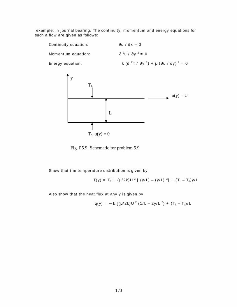
173
example, in journal bearing. The continuity, momentum and energy equations for such a flow are given as follows:
Continuity equation: ∂u / ∂x = 0
Momentum equation: ∂ 2u / ∂y 2 = 0
Energy equation: k (∂ 2T / ∂y 2) + μ (∂u / ∂y) 2 = 0
Show that the temperature distribution is given by
T(y) = To + (μ/2k)U 2 [ (y/L) – (y/L) 2] + (TL – To)y/L
Also show that the heat flux at any y is given by q(y) = ─ k [(μ/2k)U 2 (1/L – 2y/L 2) + (TL – To)/L
L
u(y) = U
To, u(y) = 0
TL
y
Fig. P5.9: Schematic for problem 5.9

174
It is given that the momentum equation is (∂2u / ∂y2) = 0 …………………………(1) With the boundary conditions : (i) at y = 0, u(y) = 0 and (ii) at y = L, u(y) = U. Integrating equation (1) twice, we have u(y) = C1y + C2 ………………………(2). Condition (i) in equation (2) gives C2 = 0. Condition (ii) in equation (2) gives U = C1L or C1= U / L. Substituting these values of C1 and C2 in equation (2) we get the velocity distribution as u(y) = (Uy) / L ………………………(3)
The energy equation is given by k(∂2T / ∂y2) = − μ (∂u / ∂y)2 …………..(4)
U
TL
T0, u(y) = 0
y
L
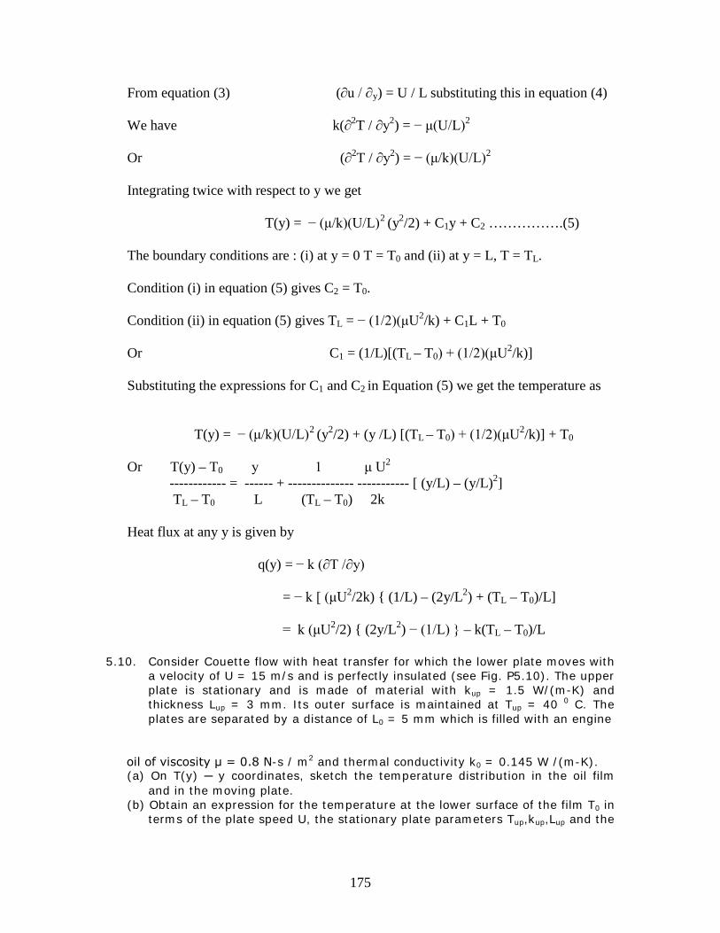
175
From equation (3) (∂u / ∂y) = U / L substituting this in equation (4) We have k(∂2T / ∂y2) = − μ(U/L)2 Or (∂2T / ∂y2) = − (μ/k)(U/L)2 Integrating twice with respect to y we get T(y) = − (μ/k)(U/L)2 (y2/2) + C1y + C2 …………….(5) The boundary conditions are : (i) at y = 0 T = T0 and (ii) at y = L, T = TL. Condition (i) in equation (5) gives C2 = T0. Condition (ii) in equation (5) gives TL = − (1/2)(μU2/k) + C1L + T0 Or C1 = (1/L)[(TL – T0) + (1/2)(μU2/k)] Substituting the expressions for C1 and C2 in Equation (5) we get the temperature as T(y) = − (μ/k)(U/L)2 (y2/2) + (y /L) [(TL – T0) + (1/2)(μU2/k)] + T0 Or T(y) – T0 y 1 μ U2 ------------ = ------ + -------------- ----------- [ (y/L) – (y/L)2] TL – T0 L (TL – T0) 2k Heat flux at any y is given by q(y) = − k (∂T /∂y) = − k [ (μU2/2k) { (1/L) – (2y/L2) + (TL – T0)/L] = k (μU2/2) { (2y/L2) − (1/L) } – k(TL – T0)/L
5.10. Consider Couette flow with heat transfer for which the lower plate moves with a velocity of U = 15 m/s and is perfectly insulated (see Fig. P5.10). The upper plate is stationary and is made of material with kup = 1.5 W/(m-K) and thickness Lup = 3 mm. Its outer surface is maintained at Tup = 40 0 C. The plates are separated by a distance of L0 = 5 mm which is filled with an engine
oil of viscosity μ = 0.8 N-s / m2 and thermal conductivity k0 = 0.145 W /(m-K).
(a) On T(y) ─ y coordinates, sketch the temperature distribution in the oil film and in the moving plate.
(b) Obtain an expression for the temperature at the lower surface of the film T0 in terms of the plate speed U, the stationary plate parameters Tup,kup,Lup and the

176
oil parameters μ, k0, L0. Calculate this temperature for the prescribed conditions.
Solution: For Couette flow the momentum equation is : d2u /dy2 = 0. Integrating twice with respect to y we have u(y) = C1y + C2 ……………………………………(1) The boundary conditions are (i) at y = 0, u(y) = U ; And (ii) at y = L0, u(y) = 0. Condition (i) in equation (1) gives C2 = U and condition (ii) in equation (1) gives C1 = − U / L0. Substituting the expressions for C1 and C2 in equation (1) we get the velocity distribution as u(y) = U [1 – (y/L0)] ……………………………..(2) The energy equation for Couette flow is
L0
Lup
oil
Stationary Plate
U
y
Fig. P5.10: Schematic for problem 5.10
Tup
Moving plate
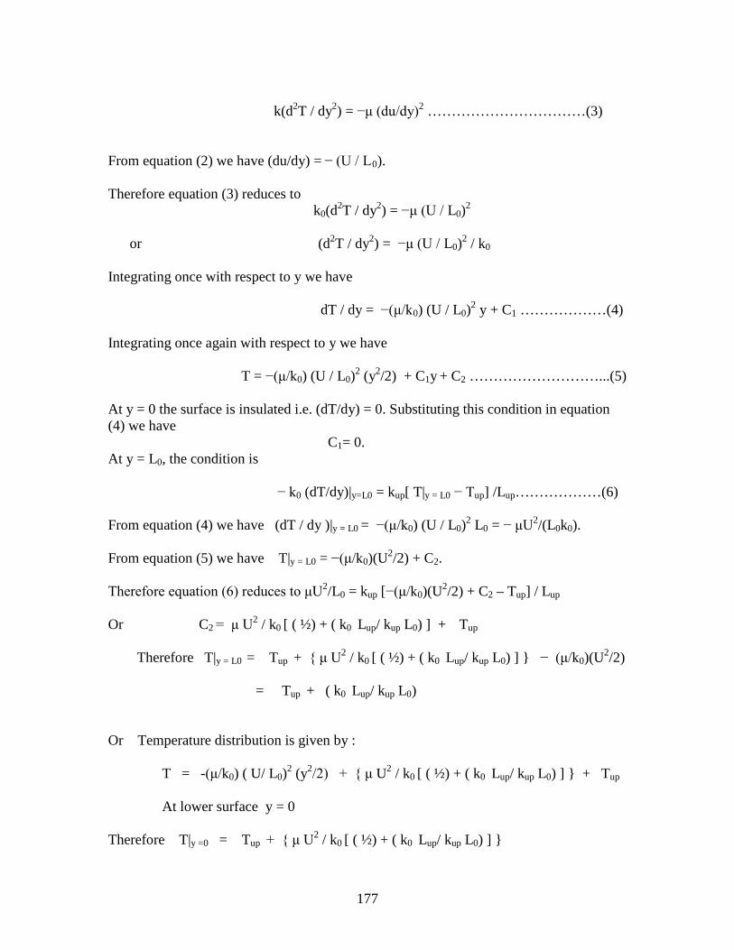
177
k(d2T / dy2) = −μ (du/dy)2 ……………………………(3)
From equation (2) we have (du/dy) = − (U / L0). Therefore equation (3) reduces to
k0(d2T / dy2) = −μ (U / L0)2 or (d2T / dy2) = −μ (U / L0)2 / k0
Integrating once with respect to y we have dT / dy = −(μ/k0) (U / L0)2 y + C1 ………………(4) Integrating once again with respect to y we have T = −(μ/k0) (U / L0)2 (y2/2) + C1y + C2 ………………………...(5) At y = 0 the surface is insulated i.e. (dT/dy) = 0. Substituting this condition in equation (4) we have C1= 0. At y = L0, the condition is − k0 (dT/dy)|y=L0 = kup[ T|y = L0 − Tup] /Lup………………(6) From equation (4) we have (dT / dy )|y = L0 = −(μ/k0) (U / L0)2 L0 = − μU2/(L0k0). From equation (5) we have T|y = L0 = −(μ/k0)(U2/2) + C2. Therefore equation (6) reduces to μU2/L0 = kup [−(μ/k0)(U2/2) + C2 – Tup] / Lup Or C2 = μ U2 / k0 [ ( ½) + ( k0 Lup/ kup L0) ] + Tup Therefore T|y = L0 = Tup + { μ U2 / k0 [ ( ½) + ( k0 Lup/ kup L0) ] } − (μ/k0)(U2/2) = Tup + ( k0 Lup/ kup L0) Or Temperature distribution is given by : T = -(μ/k0) ( U/ L0)2 (y2/2) + { μ U2 / k0 [ ( ½) + ( k0 Lup/ kup L0) ] } + Tup At lower surface y = 0 Therefore T|y =0 = Tup + { μ U2 / k0 [ ( ½) + ( k0 Lup/ kup L0) ] }

178
Chapter 6 : Forced Convection Heat Transfer
A. Hydro dynamically and thermally developed flow through tubes: 6.1. Determine the friction factor, the pressure drop and pumping power for fully
developed laminar flow of water at 21 0 C [μ = 9.8 kg/(m-s) ; ρ = 997.4 kg/m3]through a 2.5 cm diameter, 100 m long tube for a mass flow rate of 0.015 kg/s. What are the mean and maximum velocities of flow?
6.2. Determine the friction factor, the pressure drop and pumping power required
for the flow of water at 0.5 kg/s and 40 0 C through a tube of square cross section of 2 cm x 2 cm and 12 m long. What would be the corresponding values if the pipe is of equilateral-triangular cross section of side 2 cm and length 5 m ?
6.3. Water at 30 0 C with a mass flow rate of 2 kg/s enters a 2.5 cm-ID tube
whose wall is maintained at a uniform temperature of 90 0 C. Calculate the length of the tube required to heat the water to 70 0 C.
6.4. Water at 20 0 C with a mass flow rate of 5 kg/s enters a circular tube of 5 cm-
ID and 10 m long. If the tube surface is maintained at 80 0 C, determine the exit temperature of water.
6.5. Air at 27 0 C with a flow rate of 0.01 kg/s enters a rectangular tube 0.6 cm x
1.0 cm in cross section and 2 m long. The duct wall is subjected to a uniform heat flux of 5 kW/m2. Determine the outlet temperature of air and the duct surface temperature at the exit assuming that the flow is hydro dynamically and thermally developed.
6.6. Three kg/min of liquid sodium is heated from a bulk mean temperature of 400
0 C to 500 0 C, as it flows through a stainless steel tube of 5 cm-ID and 2 mm thick. The sodium is heated by a constant wall-heat flux, which maintains the tube-wall temperature at 30 0 C above the bulk mean temperature of sodium all along the length of the tube. Calculate the length of the tube required. Assume the following properties for liquid sodium. ρ = 846.7 kg/m3 ; k = 68.34 W/(m-K) ; Cp = 1.274 kJ/(kg-K) ; Pr = 0.00468
; ν =0.2937 x 10 ─ 6 m2 /s.
6.7. Consider hydro dynamically and thermally developed turbulent flow of water
with a mass flow rate of M kg/s inside a circular tube of inside diameter ‘D’. The Dittus-Boelter equation can be used to determine the heat transfer coefficient. If the tube’s inside diameter is changed from D to D/2 while the mass flow remains same, determine the resulting change in the heat transfer coefficient.
6.8. Mercury at a temperature of 100 0 C and with a velocity of 1 m/s enters a
1.25 cm ID tube, which is maintained at a uniform temperature of 250 0 C. Determine the length of the tube required.
179
B. Hydrodynamic and thermal entry lengths: 6.9. Determine the hydro dynamic entry lengths for flow at 60 0 C and at a rate of
0.015 kg/s of water, ethylene glycol and engine oil through a circular tube of 2.5 cm ID.
6.10. Determine the hydro dynamic entry length, thermal entry length and the heat
transfer coefficient for fully developed flow for engine oil at 60 0 C flowing at a rate of 0.01 kg/s through a square duct 1 cm x 1cm cross section and subjected to a uniform wall-temperature. Assume the following physical properties for the engine oil: ρ = 864 kg/m3 ; Cp = 2047 J/(kg-K) ; k = 0.14 W/(m-K) ; μ = 0.0725 kg/(m-s) ; Pr = 1050
C. Flow over a flat plate: 6.11. Atmospheric air at 25 0 C flows over both the surfaces of a flat plate 1 m long
with a velocity of 5 m/s. The plate is maintained at a uniform temperature of 750C.
(a) Determine the velocity boundary layer thickness, the surface shear stress and the heat flux at the trailing edge of the plate.
(b) Determine the drag force on the plate and the total heat transfer from the plate to air.
6.12. Air at 30 0 C flows with a velocity of 10 m/s along a flat plate 4 m long. The
plate is maintained at a uniform temperature of 130 0 C. Assuming a critical Reynolds number of 2 x 10 5 and width of plate to be 1 m determine (a) the heat flux at the trailing edge of the plate, (b) the heat transfer from the laminar portion of the plate, (c) the total heat transfer from the plate and (d) the heat transfer from the turbulent portion of the plate.
6.13. A highly conducting thin wall 2 m long separates the hot and cold air streams
flowing on both sides parallel to the plate surface. The hot stream at 250 0 C is flowing with a velocity of 50 m/s while the cold stream at 50 0 C is flowing with a velocity of 15 m/s. Calculate (a) the average heat transfer coefficients for both the air streams and the heat transfer between the two streams per metre width of the plate and (b) the local heat flux at the mid point of the plate. Assume that the wall is at the arithmetic mean of the temperature of the two streams for the purposes of calculating the physical properties of the two streams and the critical Reynolds number to be 2 x 10 5.
6.14. A flat plate of width 1 metre is maintained at a uniform temperature of 150 0
C by using independently controlled heat generating rectangular modules of thickness 10 mm and length 50 mm. Each module is insulated from its neighbours, as well as its back side.(see Fig. P 6.14). Atmospheric air at 25 0 C flows over the plate at a velocity of 30 m/s. The thermo-physical properties of the module are : k = 5.2 W/(m-K) ; Cp = 320 kJ/(kg-K) ; ρ = 2300 kg / m3.

180
(a) Find the required power generation in W/m2 in a module positioned at a
distance of 700 mm from the leading edge of the plate. (b) Find the maximum temperature in the heat generating module.
D. Flow across a cylinder: 6.15. A circular pipe of 25 mm OD is placed in an air stream at 25 0 C and 1 atm
pressure. The air moves in cross flow over the pipe at 15 /s, while the outer surface of the pipe is maintained at 115 0 C. What is the drag force exerted on the pipe per unit length of the pipe? What is the rate of heat transfer per unit length of the pipe?
6.16. A long cylindrical heating element [k = 240 W/(m-K), ρ = 2700 kg/m3 and Cp
= 900 kJ/(kg-K)] of diameter 10 mm is installed in a duct in which air moves in cross flow over the heating element at a temperature of 27 0 C with a velocity of 10 m/s.
(a) Estimate the steady state surface temperature of the heater when electrical energy is being generated at a rate of 1000 W per metre length of the cylinder.
(b) If the heater is activated from an initial temperature of 27 0 C, estimate the time required for the surface temperature to come to within 10 0 C of its steady state value.
6.17. Air at 40 0 C flows over a long 25 mm diameter cylinder with an embedded
electrical heater. Measurements of the effect of the free stream velocity V on the power per unit length P, required to maintain the cylinder surface temperature at 300 0 C yielded the following results:
V (m/s) : 1 2 4 8 12 P (W/m) : 450 658 983 1507 1963
700 mm
50 mm
150 0 C T∞ = 25 0 C u∞ = 30 m/s
10 mm
Fig. P 6.14 : Schematic for problem 6.14
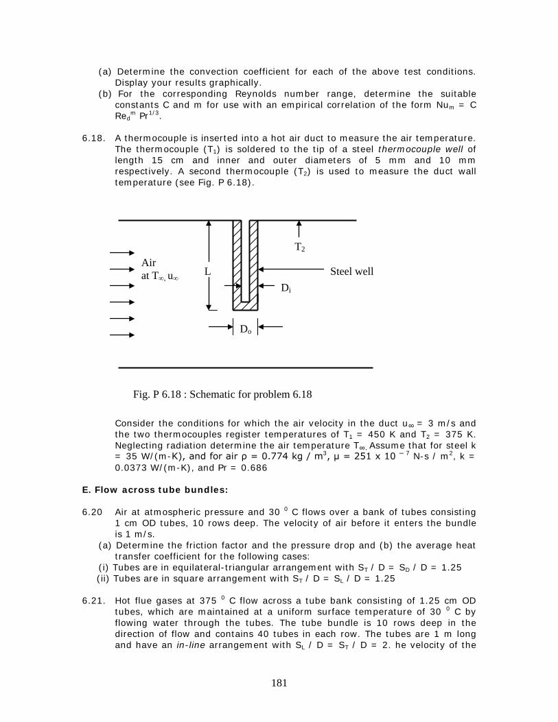
181
(a) Determine the convection coefficient for each of the above test conditions. Display your results graphically.
(b) For the corresponding Reynolds number range, determine the suitable constants C and m for use with an empirical correlation of the form Num = C Red
m Pr1/3. 6.18. A thermocouple is inserted into a hot air duct to measure the air temperature.
The thermocouple (T1) is soldered to the tip of a steel thermocouple well of length 15 cm and inner and outer diameters of 5 mm and 10 mm respectively. A second thermocouple (T2) is used to measure the duct wall temperature (see Fig. P 6.18).
Consider the conditions for which the air velocity in the duct u∞ = 3 m/s and the two thermocouples register temperatures of T1 = 450 K and T2 = 375 K. Neglecting radiation determine the air temperature T∞. Assume that for steel k = 35 W/(m-K), and for air ρ = 0.774 kg / m3, μ = 251 x 10 ─ 7 N-s / m2, k = 0.0373 W/(m-K), and Pr = 0.686
E. Flow across tube bundles: 6.20 Air at atmospheric pressure and 30 0 C flows over a bank of tubes consisting
1 cm OD tubes, 10 rows deep. The velocity of air before it enters the bundle is 1 m/s.
(a) Determine the friction factor and the pressure drop and (b) the average heat transfer coefficient for the following cases:
(i) Tubes are in equilateral-triangular arrangement with ST / D = SD / D = 1.25 (ii) Tubes are in square arrangement with ST / D = SL / D = 1.25
6.21. Hot flue gases at 375 0 C flow across a tube bank consisting of 1.25 cm OD
tubes, which are maintained at a uniform surface temperature of 30 0 C by flowing water through the tubes. The tube bundle is 10 rows deep in the direction of flow and contains 40 tubes in each row. The tubes are 1 m long and have an in-line arrangement with SL / D = ST / D = 2. he velocity of the
L
Do
Di
T2
Air at T∞, u∞ Steel well
Fig. P 6.18 : Schematic for problem 6.18
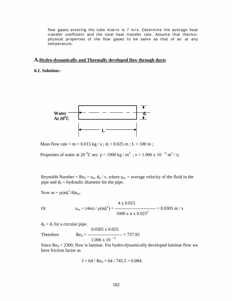
182
flow gases entering the tube matrix is 7 m/s. Determine the average heat transfer coefficient and the total heat transfer rate. Assume that thermo-physical properties of the flow gases to be same as that of air at any temperature.
A.Hydro-dynamically and Thermally developed flow through ducts 6.1. Solution:-
Reynolds Number = Red = uav dh / ν, where uav = average velocity of the fluid in the pipe and dh = hydraulic diameter for the pipe. Now m = ρ(πdi
2/4)uav.
4 x 0.015 Or uav = (4m) / ρ(πdi
2) = --------------------------- = 0.0305 m / s 1000 x π x 0.0252 dh = di for a circular pipe. 0.0305 x 0.025 Therefore Red = ----------------------- = 757.95 1.006 x 10 − 6 Since Red < 2300, flow is laminar. For hydro-dynamically developed laminar flow we have friction factor as f = 64 / Red = 64 / 745.5 = 0.084.
di
L
Water At 200C
Mass flow rate = m = 0.015 kg / s ; di = 0.025 m ; L = 100 m ; Properties of water at 20 0C are: ρ = 1000 kg / m3 ; ν = 1.006 x 10 − 6 m2 / s;
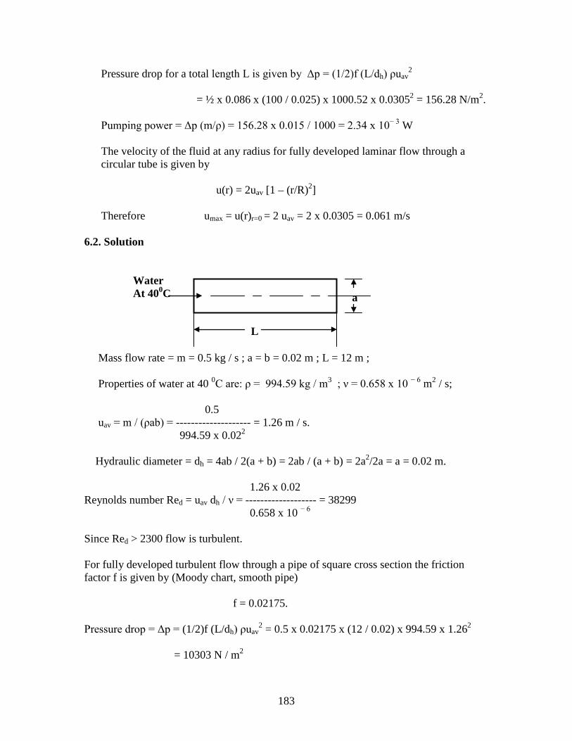
183
Pressure drop for a total length L is given by Δp = (1/2)f (L/dh) ρuav2
= ½ x 0.086 x (100 / 0.025) x 1000.52 x 0.03052 = 156.28 N/m2.
Pumping power = Δp (m/ρ) = 156.28 x 0.015 / 1000 = 2.34 x 10− 3 W
The velocity of the fluid at any radius for fully developed laminar flow through a circular tube is given by u(r) = 2uav [1 – (r/R)2] Therefore umax = u(r)r=0 = 2 uav = 2 x 0.0305 = 0.061 m/s
6.2. Solution
Mass flow rate = m = 0.5 kg / s ; a = b = 0.02 m ; L = 12 m ; Properties of water at 40 0C are: ρ = 994.59 kg / m3 ; ν = 0.658 x 10 − 6 m2 / s; 0.5 uav = m / (ρab) = -------------------- = 1.26 m / s. 994.59 x 0.022 Hydraulic diameter = dh = 4ab / 2(a + b) = 2ab / (a + b) = 2a2/2a = a = 0.02 m. 1.26 x 0.02 Reynolds number Red = uav dh / ν = ------------------- = 38299 0.658 x 10 − 6 Since Red > 2300 flow is turbulent. For fully developed turbulent flow through a pipe of square cross section the friction factor f is given by (Moody chart, smooth pipe) f = 0.02175. Pressure drop = Δp = (1/2)f (L/dh) ρuav
2 = 0.5 x 0.02175 x (12 / 0.02) x 994.59 x 1.262 = 10303 N / m2
a
L
Water At 400C

184
Pumping power = Δp x m / ρ = 10303 x 0.5 / 994.59 = 5.18 W For a tube of equilateral triangular cross section, dh = 4 {√3 x a2/4} / 3a, where a is the side of the triangle.
Hence dh = a /√3 = 0.02 / √3 = 0.0115 m 0.5 Average velocity = uav = ----------------------------- = 2.9 m/s 994.59 x (√3/4) x 0.02 2 2.9 x 0.0115 Reynolds number = Red = --------------------- = 50684 0.658 x 10 − 6 Since Red > 2300, flow is turbulent. Hence from Moody chart we have f = 0.02 Pressure drop = Δp = 0.5 x 994.59 x 2.9 2 x 0.02 x (5 / 0.0115) = 36367.4 N / m2
Pumping power = 36367.4 x 0.5 / 994.59 = 18.28 W. 6.3. Solution:
Bulk mean temperature of water = Tm = ½(Tfi + Tfo) = 0.5 x (30 + 70) = 50 0 C.
L
di Tfo Tfi
Tw
Data :- Tfi = 30 0C ; Tfo = 70 0C ; Tw = 90 0C ; m = 2 kg / s ; di = 2.5 cm = 0.025 m. To find L , assuming flow is hydrodynamically and thermally developed. For pipe of circular cross section hydraulic diameter = dh = di = 0.025.
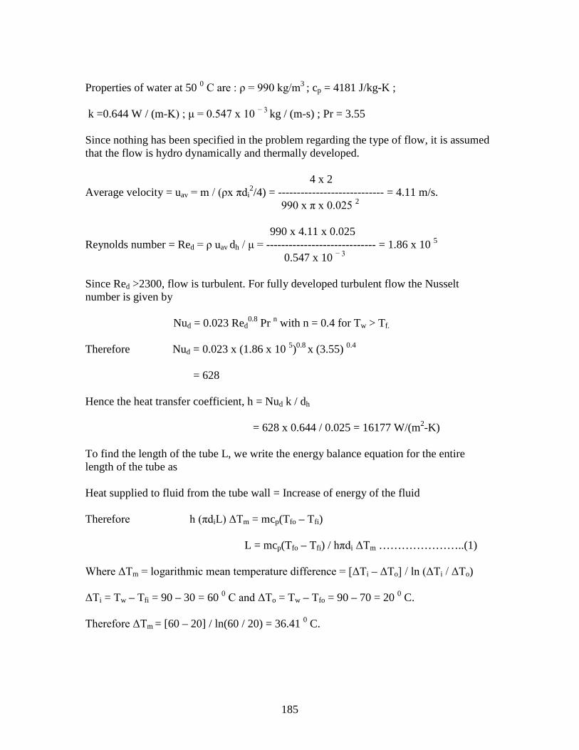
185
Properties of water at 50 0 C are : ρ = 990 kg/m3 ; cp = 4181 J/kg-K ;
k =0.644 W / (m-K) ; μ = 0.547 x 10 − 3 kg / (m-s) ; Pr = 3.55 Since nothing has been specified in the problem regarding the type of flow, it is assumed that the flow is hydro dynamically and thermally developed. 4 x 2 Average velocity = uav = m / (ρx πdi
2/4) = ---------------------------- = 4.11 m/s. 990 x π x 0.025 2 990 x 4.11 x 0.025 Reynolds number = Red = ρ uav dh / μ = ----------------------------- = 1.86 x 10 5 0.547 x 10 − 3 Since Red >2300, flow is turbulent. For fully developed turbulent flow the Nusselt number is given by Nud = 0.023 Red
0.8 Pr n with n = 0.4 for Tw > Tf. Therefore Nud = 0.023 x (1.86 x 10 5)0.8 x (3.55) 0.4 = 628 Hence the heat transfer coefficient, h = Nud k / dh = 628 x 0.644 / 0.025 = 16177 W/(m2-K) To find the length of the tube L, we write the energy balance equation for the entire length of the tube as Heat supplied to fluid from the tube wall = Increase of energy of the fluid Therefore h (πdiL) ΔTm = mcp(Tfo – Tfi) L = mcp(Tfo – Tfi) / hπdi ΔTm …………………..(1) Where ΔTm = logarithmic mean temperature difference = [ΔTi – ΔTo] / ln (ΔTi / ΔTo) ΔTi = Tw – Tfi = 90 – 30 = 60 0 C and ΔTo = Tw – Tfo = 90 – 70 = 20 0 C. Therefore ΔTm = [60 – 20] / ln(60 / 20) = 36.41 0 C.

186
[2 x 4181x (70 – 30)] Hence L = -------------------------------- = 7.23 m. 16171 x π x 0.025 x 36.41
6.4. Solution:
Trial No. 1:- Assume suitable value for Tfo noting that Tfo < Tw. Let Tfo = Tw = 60 0 C. Hence bulk mean temperature = Tm = ½(Tfi + Tfo) = 0.5 x (20 + 60) = 40 0 C. Properties of water at 40 0 C are : ρ = 994.59 kg/m3 ; cp = 4178.4 J/kg-K ; Pr = 4.34 ; ν = 0.658 x 10 − 6 m2 / s ; k = 0.628 W /(m-K). 4 x 5 Average velocity of water = uav = 4m /( πdi
2ρ) = -------------------------- π x (0.05)2 x 994.59 = 2.56 m/s. For a circular tube dh = di = 0.05 m. 2.56 x 0.05 Reynolds number = Red = uavdh / ν = ------------------------ = 1.945 x 10 5
0.658 x 10 − 6 Since Red > 2300, flow is turbulent.
Tfo Tfi water
L
di
Tw
Data :- Tfi = 20 0C ; m = 5 kg / s ; di = 0.05 m ; L = 10 m ; Tw = 80 0 C. To find Tfo.
Since Tfois not known we cannot determine the bulk fluid mean temperature to know the properties of the fluid. Hence this problem has to be solved by trial and error method as shown below.

187
Assuming the flow to be thermally and hydrodynamically developed, Nud = 0.023 Red
0.8 Pr n with n = 0.4 (as the fluid is heated) = 0.023 x (1.945 x 10 5) 0.8 (4.34) 0.4 = 704.5 704.5 x 0.628 Heat transfer coefficient = h = Nud k / dh = ---------------------- = 8848.5 W /(m2 – K). 0.05 Heat balance equation for the total length of the tube can be written as
h πdiL ΔTm = mcp[Tfo – Tfi] or h πdiL [ΔTi – ΔTo] ---------------------------- = mcp [ΔTi – ΔTo] ln[ΔTi / ΔTo] or ΔTo = ΔTi / exp {( h πdiL)/(mcp)} [80 – 20] = ---------------------------------------------------- exp{(8848.5 x π x 0.05 x 10) / (5 x 4178.4)} = 30.85 0 C. Therefore Tfo = 80 – 30.85 = 49.15 0 C. Trial 2:- Assume Tfo = 49 0 C. Therefore Tm = (49+20)/2 = 34.5 0 C. Properties of water at 34.5 0 C are : ρ = 996.22 kg/m3; cp = 4179.3 J/kg-K; Pr = 5.077; k = 0.6195 W/(m-K); ν = 0.7537 x 10 − 6 m2/s. 4 x 5 2.556 x 0.05 uav = ------------------ ------ = 2.556 m/s; Red = -------------------- = 1.696 x 10 5
π x 0.05 2 x 996.22 0.7537 x 10 − 6 Therefore Nud = 0.023 x (1.696 x 10 5) 0.8 x (5.077) 0.4 = 672.2 Hence h = 672.2 x 0.6195 / 0.05 = 8328.6 W/(m2 – K)

188
[80 – 20] Therefore Tfo = 80 − --------------------------------------------------------- exp {(8328.6 x π x 0.05 x 10) / (5 x 4179.3)} = 48 0 C which is very close to the assumed value of Tfo. Hence the iteration can be stopped. Therefore Tfo = (49 + 48) / 2 = 48.5 0 C. 6.5. Solution:
Energy balance equation for total length of the tube can be written as mcp(Tfo – Tfi) = qw 2(a+b)L Or Tfo = Tfi + [qw 2(a+b)L] / (mcp) Since Tfo is not known the property cp is read at Tfi. Therefore cp = 1005.7 J/kg-K. 2 x (0.01 + 0.006) x 2 x 5000 Therefore Tfo = 27 + -------------------------------------
0.01 x 1005.7 = 58.8 0 C. Therefore Tm = ½(Tfi + Tfo) = 0.5 x (27 + 58.8) = 42.9 0 C.
Tfo Tfi
L
qw a
b
Data :- Fluid is air ; Tfi = 27 0 C ; m = 0.01 kg/s; a = 0.01 m; b = 0.006 m; L = 2 m; qw = 5000 W / m2. find (i) Tfo ; (ii) Tw|z = L

189
Properties of air at 42.9 0 C are : ρ = 1.12 kg / m3; 1006.8 J/kg-K; ν = 17.30 x 10 − 6 m2/s; Pr = 0.7045 ; k = 0.02745 W/(m-K).(It should be noted that the variation of cp with temperature between Tfi
and Tm is very negligible and hence this problem does not require trial and error solution) 4ab 2ab 2 x 0.01 x 0.006 Hydraulic diameter = dh = ------------ = ------------- = ------------------------- 2[a + b] [a + b] [0.01 + 0.006] = 0.0075 m. 0.01 Average velocity = uav = m / [ρab] = ------------------------- = 149 m /s. 1.12 x 0.01 x 0.006 149 x 0.0075 Reynolds number = Red = uavdh / ν = --------------------- = 64595 17.3 x 10 − 6 Since Red >2300 flow is turbulent. Assuming that the flow is hydrodynamically and thermally developed we have Nud = 0.023 Red
0.8Pr n, with n = 0.4 as air is being heated. Therefore Nud = 0.023 x [64595] 0.8 x [0.7045] 0.4
= 140.9 140.9 x 0.02745 Heat transfer coefficient = h = Nud k / dh = ---------------------- = 515.7 W/(m2 – K). 0.0075 At the exit of the tube we have qw = h [Tw|z=l – Tfo] Therefore Tw|z=l = qw / h + Tfo = 5000 / 515.7 + 58.8 = 68.5 0 C 6.6.Solution: Data: Fluid is liquid sodium; m = 3/60 =0.05 kg/s; Tfi = 400 0 C; Tfo = 500 0C;di = 0.05 m ΔTi = ΔTm = ΔTo= 30 0 C; ρ = 846.7 kg/m3; k = 68.34 W/(m-K); Pr = 0.00468
cp = 1274 J/kg-K; ν = 0.2937 x 10 − 6 m2/s.
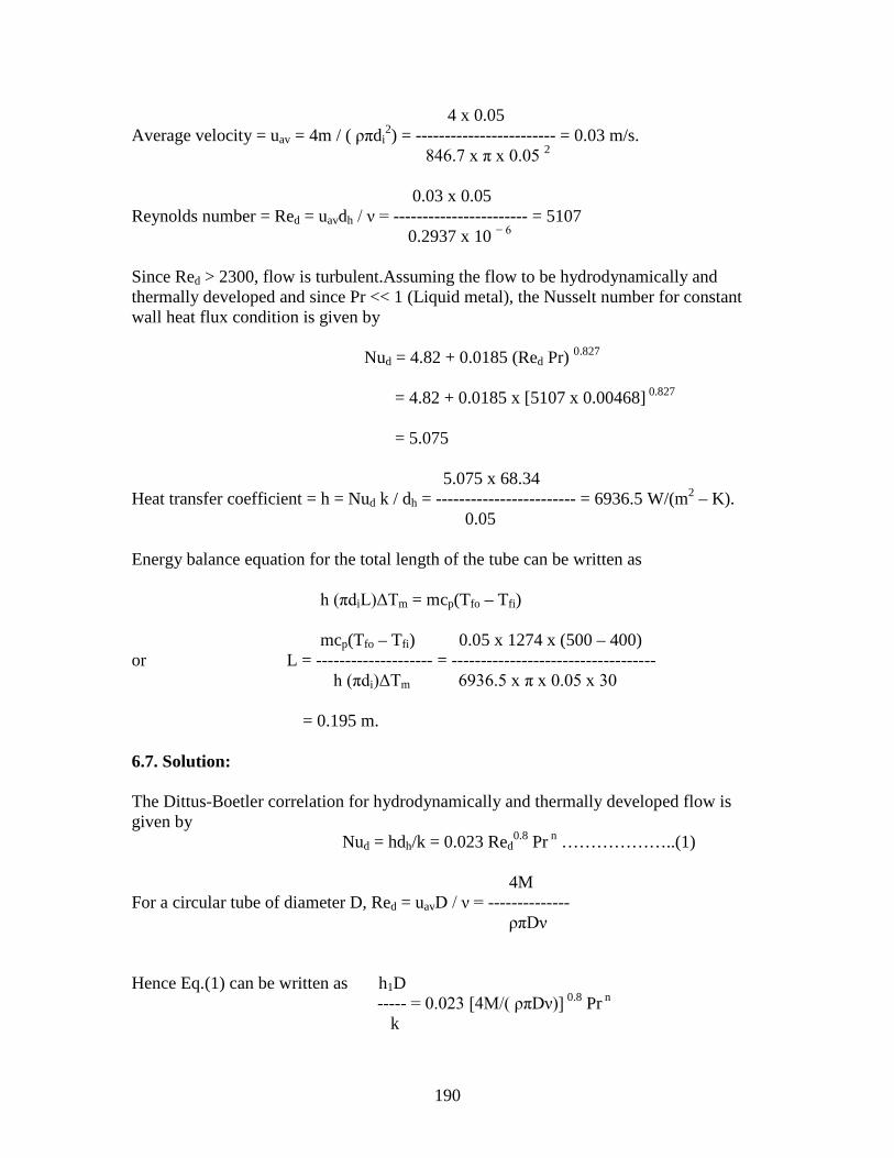
190
4 x 0.05 Average velocity = uav = 4m / ( ρπdi
2) = ------------------------ = 0.03 m/s. 846.7 x π x 0.05 2 0.03 x 0.05
Reynolds number = Red = uavdh / ν = ----------------------- = 5107 0.2937 x 10 − 6 Since Red > 2300, flow is turbulent.Assuming the flow to be hydrodynamically and thermally developed and since Pr << 1 (Liquid metal), the Nusselt number for constant wall heat flux condition is given by Nud = 4.82 + 0.0185 (Red Pr) 0.827 = 4.82 + 0.0185 x [5107 x 0.00468] 0.827 = 5.075 5.075 x 68.34 Heat transfer coefficient = h = Nud k / dh = ------------------------ = 6936.5 W/(m2 – K). 0.05 Energy balance equation for the total length of the tube can be written as h (πdiL)ΔTm = mcp(Tfo – Tfi) mcp(Tfo – Tfi) 0.05 x 1274 x (500 – 400) or L = -------------------- = ----------------------------------- h (πdi)ΔTm 6936.5 x π x 0.05 x 30 = 0.195 m. 6.7. Solution: The Dittus-Boetler correlation for hydrodynamically and thermally developed flow is given by Nud = hdh/k = 0.023 Red
0.8 Pr n ………………..(1) 4M For a circular tube of diameter D, Red = uavD / ν = -------------- ρπDν
Hence Eq.(1) can be written as h1D ----- = 0.023 [4M/( ρπDν)] 0.8 Pr n
k
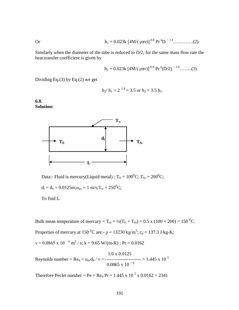
191
Or h1 = 0.023k [4M/( ρπν)] 0.8 Pr nD − 1.8………….(2) Similarly when the diameter of the tube is reduced to D/2, for the same mass flow rate the heat transfer coefficient is given by h2 = 0.023k [4M/( ρπν)] 0.8 Pr n(D/2) − 1.8……..(3) Dividing Eq.(3) by Eq.(2) we get h2/ h1 = 2 1.8 = 3.5 or h2 = 3.5 h1. 6.8. Solution:
Bulk mean temperature of mercury = Tm = ½(Tfi + Tfo) = 0.5 x (100 + 200) = 150 0C. Properties of mercury at 150 0C are:- ρ = 13230 kg/m3; cp = 137.3 J/kg-K; ν = 0.0865 x 10 − 6 m2 / s; k = 9.65 W/(m-K) ; Pr = 0.0162 1.0 x 0.0125 Reynolds number = Red = uavdh / ν = ----------------------- = 1.445 x 10 5 0.0865 x 10 − 6 Therefore Peclet number = Pe = Red Pr = 1.445 x 10 5 x 0.0162 = 2341
Tfi Tfo
Tw
L
di
Data:- Fluid is mercury(Liquid metal) ; Tfi = 1000C; Tfo = 2000C; di = dh = 0.0125m;uav = 1 m/s;Tw = 2500C; To find L

192
Since Red > 2300, flow is turbulent. Therefore for liquid metal flow subjected to uniform wall-temperature Nusselt number is given by Nud = 5.0 + 0.025 Pe 0.8 = 5.0 + 0.025 x 2341 0.8 = 17.4 15.97 x 11.425 Heat transfer coefficient, h = Nudk/dh = -------------------- = 13433 W/(m2-K) 0.0125 ΔTi = Tw – Tfi = 250 – 100 = 150 0 C ; ΔTo = Tw – Tfo = 250 – 200 = 50 0 C. Mean temperature difference = ΔTm = [ΔTi − ΔTo] / ln(ΔTi / ΔTo) = [150 – 50] / ln(150 / 50) = 91 0 C Mass flow rate of mercury = m = ρ(πdi
2/4)uav = 13230 x (π x 0.0125 2/4) x 1.0 = 1.624 kg/s Energy balance equation for the total length of the pipe is given by h πdiL ΔTm = mcp(Tfo – Tfi) mcp(Tfo – Tfi) 1.624 x 137.3 x (200 – 100) Therefore L = ------------------ = ------------------------------------ h πdi ΔTm 13433 x π x 0.0125 x 91 = 0.465 B Hydrodynamic and Thermal Entry Lengths 6.9. Solution: Data:- Tfi = 60 0C ; m = 0.015 kg / s; di = dh = 0.025 m.
(i) Fluid is water. Hence at 60 0 C, ρ = 985.46 kg / m3 ; ν = 0.478 x 10 − 6 m2 / s. 4 x 0.015 Average velocity = uav = 4m / ρπdi
2 = -------------------------- = 0.032 m/s. 985.46 x π x 0.025 2 0.031 x 0.025 Reynolds number = Red = uavdh / ν = --------------------- = 1674 0.478 x 10 − 6

193
Since Red < 2300, flow is laminar. Hence the hydrodynamic entrance length Lh for a circular pipe is given by Lh / dh -------- = 0.056 Red Therefore Lh = 0.056 Red dh = 0.056 x 1674 x 0.025 = 2.34 m (ii)Fluid is ethylene glycol: ρ = 1087.66 kg/m3 ; ν = 4.75 x 10 − 6 m2/s. 4 x 0.015 Average velocity = uav = 4m / ρπdi
2 = -------------------------- = 0.0281 m/s. 1087.66 x π x 0.025 2 0.0281 x 0.025 Reynolds number = Red = ---------------------------- = 147.9 4.75 x 10 − 6 Since Red < 2300, flow is laminar. Therefore Lh = 0.056 Red dh = 0.056 x 147.9 x 0.025 = 0.21 m. (iii) Fluid is engine oil; ρ = 864.04 kg/m3 ; ν = 0.839 x 10 − 4 m2/s. 4 x 0.015 Average velocity = uav = 4m / ρπdi
2 = -------------------------- = 0.0354 m/s. 864.04 x π x 0.025 2 0.0354 x 0.025 Reynolds number = Red = ---------------------------- = 10.55 0.839 x 10 − 4 Therefore Lh = 0.056 Red dh = 0.056 x 10.55 x 0.025 = 0.013 m. 6.10.Solution: Data: Fluid is engine oil ; Tfi = 60 0C; m = 0.01 kg/s; square duct with a = 0.01m ; ρ = 864 kg/m 3; cp = 2047 J/kg-K; k = 0.14 W/(m-K); μ = 0.0725 kg/(m-s); Pr = 1050. To find (i) Lh ;(ii)Lt ; (iii) h for fully developed flow. (i) Hydraulic diameter = dh = 4a 2 /(4a) = a = 0.01 m.
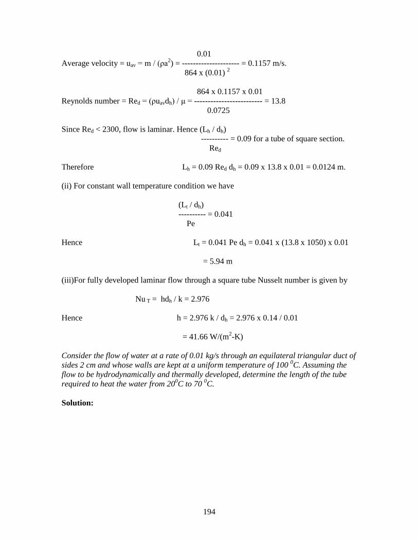
194
0.01 Average velocity = uav = m / (ρa2) = --------------------- = 0.1157 m/s. 864 x (0.01) 2 864 x 0.1157 x 0.01 Reynolds number = Red = (ρuavdh) / μ = ------------------------- = 13.8 0.0725 Since Red < 2300, flow is laminar. Hence (Lh / dh) ---------- = 0.09 for a tube of square section. Red Therefore Lh = 0.09 Red dh = 0.09 x 13.8 x 0.01 = 0.0124 m. (ii) For constant wall temperature condition we have (Lt / dh) ---------- = 0.041 Pe Hence Lt = 0.041 Pe dh = 0.041 x (13.8 x 1050) x 0.01 = 5.94 m (iii)For fully developed laminar flow through a square tube Nusselt number is given by Nu T = hdh / k = 2.976 Hence h = 2.976 k / dh = 2.976 x 0.14 / 0.01 = 41.66 W/(m2-K) Consider the flow of water at a rate of 0.01 kg/s through an equilateral triangular duct of sides 2 cm and whose walls are kept at a uniform temperature of 100 0C. Assuming the flow to be hydrodynamically and thermally developed, determine the length of the tube required to heat the water from 200C to 70 0C. Solution:
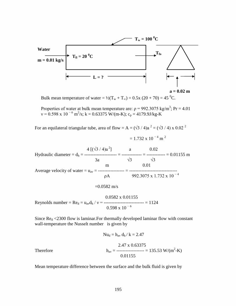
195
For an equilateral triangular tube, area of flow = A = (√3 / 4)a 2 = (√3 / 4) x 0.02 2 = 1.732 x 10 − 4 m 2 4 [(√3 / 4)a 2] a 0.02 Hydraulic diameter = dh = --------------------- = ------------- = ------------ = 0.01155 m 3a √3 √3 m 0.01 Average velocity of water = uav = ----------------- = ------------------------------- ρA 992.3075 x 1.732 x 10 − 4 =0.0582 m/s 0.0582 x 0.01155 Reynolds number = Red = uavdh / ν = -------------------------- = 1124 0.598 x 10 − 6 Since Red <2300 flow is laminar.For thermally developed laminar flow with constant wall-temperature the Nusselt number is given by Nud = hav dh / k = 2.47 2.47 x 0.63375 Therefore hav = ------------------ = 135.53 W/(m2-K) 0.01155 Mean temperature difference between the surface and the bulk fluid is given by
Tfi = 20 0C Tfo
L = ?
a = 0.02 m
Tw = 100 0C
Water m = 0.01 kg/s
Bulk mean temperature of water = ½(Tw + T∞) = 0.5x (20 + 70) = 45 0C. Properties of water at bulk mean temperature are: ρ = 992.3075 kg/m3; Pr = 4.01 ν = 0.598 x 10 − 6 m2/s; k = 0.63375 W/(m-K); cp = 4179.9J/kg-K

196
ΔTm = [ΔTi – ΔTo] / ln[ΔTi / ΔTo] Now ΔTi = Tw – Tfi = 100 – 20 = 80 0C; ΔTo = Tw – Tfo = 100 – 70 = 30 Hence ΔTm = [80 – 30] / ln{80/30} = 50.1 0C. Rate of heat transfer to water = Q = mcp(Tfo – Tfi) = 0.01 x 4179.9 x (70 – 20) = 2090 W But Q = havPL ΔTm, where P is the perimeter of the duct = 3a Hence Q = hav 3aL ΔTm Q 2090 Or L = -------------------- = ------------------------------ hav 3a ΔTm 135.53 x 3 x 0.02 x 50.1 = 5.13 m
C Flow over a flat plate: 6.11. Solution:
x L
Tw
u∞, T∞
Data:- Fluid is air; u∞ = 5 m/s; T∞ = 25 0 C; L = 1 m; Tw = 75 0 C. Mean temperature = ½(Tw + T∞) = 0.5 x (75 + 25) = 50 0 C. Properties of air at 50 0 C are : ρ = 1.093 kg/m3; ν = 18.02 x 10 − 6 m
2 /s; Pr =0.703 k = 0.028 W/(m-K).
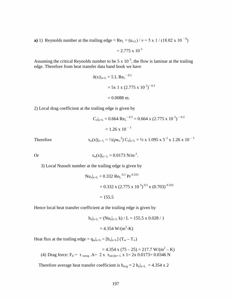
197
a) 1) Reynolds number at the trailing edge = ReL = (u∞L) / ν = 5 x 1 / (18.02 x 10 − 6) = 2.775 x 10 5 Assuming the critical Reynolds number to be 5 x 10 5, the flow is laminar at the trailing edge. Therefore from heat transfer data hand book we have δ(x)|x=L = 5 L ReL
− 0.5 = 5x 1 x (2.775 x 10 5)− 0.5 = 0.0088 m. 2) Local drag coefficient at the trailing edge is given by Cx|x=L = 0.664 ReL
− 0.5 = 0.664 x (2.775 x 10 5) − 0.5 = 1.26 x 10 − 3
Therefore τw(x)|x= L = ½(ρu∞
2) Cx|x=L = ½ x 1.095 x 5 2 x 1.26 x 10 − 3 Or τw(x)|x= L = 0.0173 N/m 2.
3) Local Nusselt number at the trailing edge is given by Nux|x=L = 0.332 ReL
0.5 Pr 0.333 = 0.332 x (2.775 x 10 5) 0.5 x (0.703) 0.333 = 155.5 Hence local heat transfer coefficient at the trailing edge is given by hx|x=L = (Nux|x=L k) / L = 155.5 x 0.028 / 1 = 4.354 W/(m2-K) Heat flux at the trailing edge = qw|x=L = [hx|x=L] (Tw – T∞) = 4.354 x (75 – 25) = 217.7 W/(m2 – K)
(4) Drag force: Fd = τ wavg .A= 2 x τw(x)|x= L x 1= 2x 0.0173= 0.0346 N
Therefore average heat transfer coefficient is havg = 2 hx|x=L = 4.354 x 2

198
=8.708 W/(m2 – K) and Average heat flus = qw = [havg] (Tw – T∞)= 8.708 x 50 = 435.4 W/(m2 – K) 6.12. Solution:-
10 x 4 ReL = u∞L / ν = -------------------------- = 1.86 x 10 − 6
21.48 x 10 − 6
Since ReL > Recr flow is turbulent at the trailing edge. For turbulent flow of air over a flat plate the local Nusselt number is given by Nux = 0.0296 Rex
0.8 Pr 1/3. Hence Nux|x=L = 0.0296 x [1.86 x 10 6] 0.8 (0.692) 1/3 = 2721 2721 x 0.03047 Therefore [hx|x=L] L / k = 2803 or hx|x=L = ---------------------- = 21 W /(m2-K) 4 Heat flux at the trailing edge = qw(x)|x=L = [hx|x=L] (Tw – T∞)
L = 4 m x
u∞ = 10 m/s (air) T∞ = 30 0 C Tw = 130 0 C
To find :- (a) qw(x)|x=L; (b) Qlaminar; (c) Qturbulent assuming Recr = 2 x 10 5
Mean film temperature = ½(Tw + T∞) = 0.5 x (130 + 30) = 80 0C. Properties of air at mean film temperature are: ν =21.48 x 10 − 6 m2/s; Pr = 0.692 k = 0.03047 W /(m-K).
W=1 m

199
= 21 x (130 – 30) = 2100 W / m2.
(b) Recr = u∞ xcr / ν. Recr ν 2 x 10 5 x 20.76 x 10 − 6 Or xcr = --------- = ------------------------------- = 0.415 m u∞ 10 Hence flow is laminar up to xcr. Average Nusselt number for the laminar region is given by [Nuav] laminar = 0.664 Recr
0.5 Pr 1/3
= 0.664 x [2 x 10 5] 0.5(0.697) 1/3 = 263.3 Hence average heat transfer coefficient for the laminar region is 263.3 x 0.03003 [hav]laminar = [Nuav] laminar k / xcr = ----------------------- 0.415 = 19.00 W /(m2 –K) Heat transfer rate from laminar portion = Qlaminar = [hav]laminar [x cr W] (Tw – T∞) = 19.0 x [ 0.415 x 1] x (130 – 30) = 789.0 W (c)Average Nusselt number for the entire length of the plate is given by Nuav = Pr 1/3 [ 0.037ReL
0.8 – A] Where A = 0.037Recr
0.8 – 0.664Recr0.5.
For this problem A = 0.037 x [2 x 10 5] 0.8 – 0.664 x [2 x 10 5] 0.5 = 356 Therefore Nuav = (0.697) 1/3 [0.037 x {1.93 x 10 6} 0.8 – 356] = 3180 3180 x 0.03047 Hence hav = Nuav k / L = ----------------------- 4 = 24.2 W/(m2 – K)

200
Qtotal = hav (LW)(Tw – T∞) = 24.2 x (4 x 1) x (130 – 30) = 9680 W Qturbulent = Qtotal – Qlaminar = 9680 – 789 = 8891 W 6.13. Solution:
(i) Mean film temperature for the hot fluid = ½(Tw + T∞1) = 0.5 x (150 + 250) = 200 0C. Properties of air at 200 0C are: ν = 34.85 x 10 − 6 m2 / s;k = 0.03931 W/(m-K);Pr = 0.68 Reynolds number at the trailing edge of the plate = ReL = u∞1L / ν 50 x 2 Or ReL = ------------------- 34.85 x 10 − 6 = 2.865 x 10 6
Since ReL > Recr, flow is partly laminar and partly turbulent. Therefore the average Nusselt number is given by Nuav = Pr 1/3[0.037 ReL
0.8 – A] Where A = 0.037 Recr
0.8 – 0.664 Recr 0.5.
Or A = 0.037 x [2 x 10 5]0.8 – 0.664 x [2 x 10 5] 0.5 = 347.25
Hot air at T∞1 =250 0 C, u∞1 = 50 m/s
Cold air at T∞2 = 50 0C, u∞2 = 15 m / s
Tw = ½( T∞1+ T∞2) = 150 0 C
L = 2 m
Additional data:- Recr = 2 x 10 5 To find (i) hav for the hot surface ; (ii) hav for the cold surface ; (iii) qw(x)|x=L/2

201
Hence Nuav = (0.68) 1/3 [0.037 x (3.028 x 10 6) 0.8 – 347.25] = 4465 4465 x 0.0391 Hence for the hot surface [hav] hot = Nuav k / L = ---------------------- 2 = 987.76 W/(m2-K) (ii) Mean film temperature for the cold surface = ½(150 + 50) = 100 0C. Properties of air at the mean film temperature are: ν = 23.33 x 10 − 6 m2/s; Pr = 0.693 k = 0.03184 W/(m-K) 15 x 2 ReL = u∞2L / ν = -------------------------- = 1.286 x 10 6
23.33 x 10 − 6 Therefore Nuav = (0.693) 1/3[0.037 x (1.286 x 10 6) 0.8 – 347] = 2219 2219 x 0.03184 Hence for the cold surface [hav]cold = -------------------- = 35.33 W/(m2-K). 2 (iii) The rate of heat transfer from the hot air stream to cold air stream is given by Q = (T∞1 - T∞2) / [Rc1 + R + Rc2] Where Rc1 = Thermal resistance offered by hot surface for convection, Rc2 = Thermal resistance offered by cold surface for convection, and R = Thermal resistance offered by the plate for conduction. 1 Now Rc1 = 1 / [hav]hot A = ------------------- = 0.00554 m2 – K / W. 90.3 x (2 x 1) 1 Similarly Rc2 = 1 / [hav]cold A = -------------------- = 0.01415 m2 – K / W. 35.33 x (2 x 1) R = L / Ak . Since k is not given it is assumed that k is very large i.e R = 0.

202
Therefore Q = [250 – 50] / [ 0.00554 + 0.01415] = 10,157 W. (iv) At mid point of the plate x = L / 2. Therefore for the hot fluid Re|x=L/2 = ½ ReL = 0.5 x 2.865 x 10 6 = 1.4325 x 10 6 which is > Recr. Therefore flow is turbulent at mid point of the plate. Hence [Nu|x=L/2]hot = 0.037 [Re|x=L/2] 0.8 Pr 1/3
= 0.037 x [1.5014 x 10 6] 0.8 x (0.6815) 1/3 = 2739 Hence [hx|x=L/2]hot = 2739 x 0.03931 / 1 = 107.7 W/(m2-K). Similarly [Nu|x=L/2]cold = 0.037 x [0.5 x 1.286 x 10 6] 0.8 x (0.693) 1/3 = 1451 Hence [hx|x=L/2]cold = 1451 x 0.03184 / 1 = 46.2 Heat flux at the mid point of the plate is given by qw(x)|x=L/2 = [hx|x=L/2]hot [T∞1 – Tw] = [hx|x=L/2]cold [Tw - T∞2] CT∞1 + T∞2 [hx|x=L/2]hot 107.7 Therefore Tw = ----------------------- ; C = ---------------- = ---------- = 2.33 1 + C [hx|x=L/2]cold 46.2 (2.33 x 250) + 50 Hence Tw = -------------------------- = 187.41 0C 1 + 2.375 Therefore qw(x)|x=L/2 = 107.7 x [250 –187.41] = 6743 W/m2 Also check for qw(x)|x=L/2 ; qw(x)|x=L/2 = 46.2 x (187.41 – 50) = 6348.34 W/m2 6.14. Solution:

203
Reynolds number at x1 = Rex1 = u∞x1/ ν = 30 x 0.7 / (21.79 x 10 − 6) = 9.637 x 10 5. Similarly Rex2 = u∞x2 / ν = 30 x 0.75 / (21.79 x 10 − 6) = 10.325 x 10 5 Since Rex1 > Recr, the flow is turbulent at x1 and the flow will be turbulent over the module under consideration. Therefore the average heat transfer coefficient for the module can be written as x2 [hav]m = {1 / (x2 – x1)} ∫ hxdx
x1
= {1 / (x2 – x1)} ∫(Nux k/x)dx x2 = {1 / (x2 – x1)} ∫{k[ 0.037 (Rex)0.8 – 871]Pr 1/3 /x}dx x1 k Pr 1/3 x2
= ---------------- { ∫ [0.037 (u∞/ν)0.8 x − 0.2 – 871/x]dx } (x2 – x1) x1 k Pr 1/3 = ---------------- {0.037 (u∞/ν)0.8 ∫ x − 0.2 dx - 871∫ (dx /x) } (x2 – x1) k Pr 1/3 = ---------------- { 0.04625[Rex2
0.8 – Rex10.8] – 871 ln (x2 / x1)}
(x2 – x1)
X1 = 700 mm
X2 = 750 mm
Tw = 150 0 C Air with u∞ = 30 m/s,T∞ = 25 0C
10 mm
Insulated
Properties of the module: km = 5.2 W/(m-K); cpm = 320 kJ/kg-K; ρm = 2300 kg/m3. Mean film temperature = ½(Tw + T∞) = 0.5 x(25 + 150) = 87.5 0C. Properties of air at 87.5 0C are : ν = 21.79 x 10 − 6 m2/s; k = 0.03075 W/(m-K); Pr = 0.695. Assume Recr = 5 x 10 5

204
0.03075 x (0.695)1/3{0.04625[(10.327 x105)0.8 –(9.325 X 10⁵)0.8] – 871 ln (0.75/0.7)} = ------------------------------------------------------------------------------------------------------- (0.75 – 0.7) = 95.16 W / (m2-K) For the module, power generation = qw = [hav]m {Tw - T∞} = 95.16 x (150 – 25) = 11895 W/m2 = 11.895 kW/ m2 (b) Since the bottom surface of the module is insulated, all the heat generated in the module is transferred to air from the top surface of the module. Hence if q’’’ is the heat generated per unit volume then q’’’ (x2 – x1)δW = qw(x2 – x1)W, where δ is the thickness of the module. Therefore q’’’ = qw / δ = 11895 / 0.001 = 11.895 x 10 6 W/m3. For the module the governing conduction equation is d2T/dy2 + q’’’ / k = 0 ………………………….(a) where y is the coordinate measured in the direction of the thickness of the module. The boundary conditions are (i) at y = 0, the surface is insulated i.e. dT/dy = 0 and at y = δ, T = Tw. The solution of Eq.(a) subject to the boundary conditions is given by T(y) + q’’’y2 / 2k = Tw + q’’’δ2 / 2k Since the bottom surface is insulated, the maximum temperature of the module will be at the bottom surface (y = 0) and is therefore given by Tmax = Tw + q’’’δ2 / 2k 11.895 x 106 x (0.001)2
= 150 + ----------------------------- 2 x 5.2 = 151.1 0C D) Flow across a cylinder

205
6.15. Solution:
(i) Reynolds number = Red = u∞d / ν = 15 x 0.025 / 20.05 x 10 −6 = 18703 From the chart the drag coefficient ,CD = 1.2 Therefore drag force = FD = ½(ρu∞
2)LD CD = 0.5 x 1.0231 x 152 x 1 x 0.025 x 1.2 = 3.453 N (ii) From Heat transfer data hand book for gases the average Nusselt number is given by ( μw = μ∞ can be considered for air ) Nuav = havD/k = (0.4Red
0.5 + 0.06 Red 2/3) Pr0.4
= (0.4 x 18703 0.5 + 0.06 x 18703 2/3) x (0.699) 0.4 = 84.04 84.04 x 0.0295 Therefore hav = Nuav k/d = -------------------- = 99.17 W/(m2-K) 0.025 Heat transfer = Q = havπdL(Tw – T∞) = 99.17 x π x 0.025 x 1 x (115 – 25) = 701 W
d = 0.025 m L
u∞ = 15 m/s; T∞ = 25 0 C Tw = 1150C
Mean film temperature = ½ (Tw + T∞) = 0.5 x (115 + 25) = 70 0C. Properties of air at 70 0C are: ρ = 1.0231 kg/m3; ν = 20.05 x 10 −6m2/s; Pr = 0.699; k = 0.0295 W/(m-K); To find (i) Drag force FD ; (ii) Q

206
6.16 Solution:
Since Tw is not known it is not possible to read the properties at the mean film temperature. Hence the problem has to be solved by trail and error procedure. Trial 1:- Calculations are started using the properties of air at T∞. Properties of air at 270C are: ρ = 1.1774 kg/m3; cp = 1.0057 kJ/kg-K; ν = 15.68 x 10 − 6 m2/s; k = 0.02624 W/(m-K); Pr = 0.708 10 x 0.01 Red = u∞D / ν = ---------------------- = 6377.5 15.68 x 10 − 6
( μw = μ∞ can be considered for air ) Therefore Nuav = havD/k = (0.4Red
0.5 + 0.06 Red 2/3) Pr0.4
= (0.4 x 6377.50.5 + 0.06 x 6377.5 2/3) x (0.708) 0.4 = 45.79 45.79 x 0.02624 Therefore hav = Nuav k/D = ------------------------- = 120.15 W/(m2- K) 0.01 Now Qw = hav πDL (Tw – T∞)
u∞ = 10 m/s; T∞ = 27 0C
D = 0.01 m
Qw
Given:- Qw = 1000 W/m; ks = 240 W/(m-K); ρs = 2700 kg/m3; Cps = 900 kJ/kg-K To find (i) Tw under steady state condition (ii) time ‘t’ required for the surface to reach a temperature of (Tw – 10) 0C
L

207
Or Tw = T∞ + Qw /hav πDL = 27 + 1000 / (120.15 x π x 0.01 x 1) = 291.930 C Trial 2:- Assume Tw = 291.93 0C .Mean film temperature = ½(291.93 +27) = 159.5 0C. Properties of air at 159.50C are: ν = 30.09 x 10 − 6 m2/s; k = 0.03640 W/(m-K); Pr = 0.682. 10 x 0.01 Red = u∞D / ν = ---------------------- = 3323.4 30.09 x 10 − 6 Nuav = (0.4 x 3323.4 0.5 + 0.06 x 3323.4 2/3) x (0.682) 0.4 = 31.25 Hence hav = 31.25 x 0.03640 / 0.01 = 113.75 W/(m2-K) Therefore Tw = 27 + 1000 / (113.75 x π x 0.01 x 1) = 306.8 0C. Since this value of Tw is considerably different from the value got in the first trial, one more iteration is required. Trial 3:- Assume Tw = 303 0 C. Mean film temperature = 0.5 (303 + 27) = 165 0 C. Properties of air at 165 0 C are: ν = 30.88 x 10 − 6 m2/s; k = 0.0369 W/(m-K); Pr = 0.682 10 x 0.01 Red = u∞D / ν = ---------------------- = 3238.34 30.88x 10 − 6 Nuav = (0.4 x 3238.34 0.5 + 0.06 x 3238.34 2/3) x (0.682) 0.4 = 30.8 Hence hav = 30.8 x 0.0369 / 0.01 = 113.65W/(m2-K) Therefore Tw = 27 + 1000 / (113.65 x π x 0.01 x 1) = 307 0C which is very close to the assumed value of 303 0 C and hence the iteration can be stopped. Therefore Tw = 307 0C. E. Flow across tube bundles

208
6.20.Solution: Case (i) Square Arrangement
Since the surface temperature of the tubes is not known properties of air are evaluated at T∞. Hence properties of air at 30 0C are: ρ = 1.1774 kg/m3; μ = 1.983 x 10 − 5 kg/(m-s); cp = 1005.7 J/kg-K; k = 0.02624 W/(m-K); Pr = 0.708 (i) For square arrangement the maximum velocity is given by ST / D 1.25 Umax = u∞ ------------------ = 1 x ---------------- [ST / D – 1] [ 1.25 – 1] = 5 m/s. Gmax = ρUmax = 1.1774 x 5 = 5.887 kg/(m2-s) 0.01 x 5.887 Reynolds number = Re = DGmax / μ = ------------------------ = 2969 1.983 x 10 − 5 From the graph friction factor f = 5.5 and Z = 1 for square arrangement as ST = SL.
N (Gmax) 2 10 x (5.887) 2
Now Δp = f ---------------- Z = 5.5 x ------------------------- x 1.0 ρ 1.1774
SL
ST
Row 1 Row 2 Row 3
D
Data:- T∞ = 30 0 C; D = 0.01 m; N = 10; u∞ = 1 m/s; ST / D = SL / D = 1.25 To find (i) friction factor,f; (ii) pressure drop Δp ; (iii) hav
u∞,T∞∞

209
= 1619 N / m2 (ii) For N ≥ 20 the average Nusselt number is given by Nuav = c2Rem Pr0.36 (Pr/Prw)n Here c2 = 0.27 ; m = 0.63 ; n = 0. Therefore Nuav = 0.27 x (2969) 0.63 (0.708)0.36 = 36.74 Since N <20, the above value of Nuav has to be multiplied by a correction factor. Hence [ Nuav] N=10 = c3[Nuav]N≥ 20 For Re = 2969 and N = 10 from the graph c3 = 0.98 Therefore [ Nuav] N=10 = 0.98 x 36.74 = 36 Therefore hav = 36 x 0.02624 / 0.01 = 94.5 W/(m2-K) Case (ii); Equilateral Triangular Arrangement:
ST / D Maximum velocity Umax = u∞ ------------------ = 5 m/s as calculated above [ST / D – 1]
ST SD
u∞,T∞
Given: ST / D = SD / D = 1.25
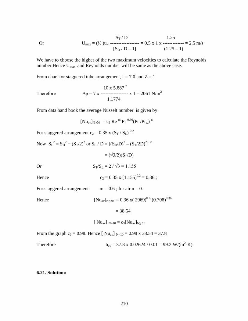
210
ST / D 1.25 Or Umax = (½ )u∞ ------------------ = 0.5 x 1 x ------------- = 2.5 m/s [SD / D – 1] (1.25 – 1) We have to choose the higher of the two maximum velocities to calculate the Reynolds number.Hence Umax and Reynolds number will be same as the above case. From chart for staggered tube arrangement, f = 7.0 and Z = 1 10 x 5.887 2
Therefore Δp = 7 x ----------------- x 1 = 2061 N/m2
1.1774 From data hand book the average Nusselt number is given by [Nuav]N≥20 = c2 Re m Pr 0.36(Pr /Prw) n For staggered arrangement c2 = 0.35 x (ST / SL) 0.2 Now SL
2 = SD2 − (ST/2)2 or SL / D = [(SD/D)2 – (ST/2D)2] ½
= (√3/2)(ST/D) Or ST/SL = 2 / √3 = 1.155 Hence c2 = 0.35 x [1.155]0.2 = 0.36 ; For staggered arrangement m = 0.6 ; for air n = 0. Hence [Nuav]N≥20 = 0.36 x( 2969)0.6 (0.708)0.36 = 38.54 [ Nuav] N=10 = c3[Nuav]N≥ 20 From the graph c3 = 0.98. Hence [ Nuav] N=10 = 0.98 x 38.54 = 37.8 Therefore hav = 37.8 x 0.02624 / 0.01 = 99.2 W/(m2-K).
6.21. Solution:

211
Mean film temperature = 0.5 x (375 + 30) = 202.5 0C. Properties of air at 202.5 0C are: ρ = 0.9403 kg/m3; cp = 1.0115 kJ/(kg-K); μ = 2.1805 x 10 − 5 m2/s; k = 0.03184 W/(m-K); Pr = 0.693 For inline arrangement Umax = u∞ (ST/D) / [(ST/D) − 1] = 7 x 2 /(2 – 1) = 14 m/s. Mass velocity = Gmax = ρ Umax = 0.9403 x 14 = 13.164 kg/(m2-s) 0.0125 x 13.164 Reynolds number = Re = DGmax / μ = ---------------------- = 7546 2.1805 x 10 − 5 The average Nusselt number for N ≥ 20 is given by [Nuav]N≥20 = c2 RemPr0.36 For in-line arrangement from data hand book, c2 = 0.27 and m = 0.63 Therefore [Nuav]N≥20 = 0.27 x (7546) 0.63 x (0.693)0.36 = 170 [ Nuav] N=10 = c3[Nuav]N≥ 20 with c3 = 0.96 Hence [ Nuav] N=10 = 0.96 x 170 = 163.2 163.2 x 0.03184 Average heat transfer coefficient = hav = [ Nuav] N=10 k / D = ---------------------- 0.0125
Hot gases at u∞,T∞
ST
SL
D
Data:- T∞ = 375 0C; u∞ = 7 m/s; Tw = 30 0C; Number of rows = N = 10 ; D = 0.0125 m; number of tubes in each row = m = 40; L = 1 m ; In-line arrangement; SL/D = ST/D = 2. To find:- (i) hav ; (ii) Q
212
= 416 W/(m2-K). Energy balance between the tubes surfaces and hot gases can be written as Heat transfer from hot gases to the tube surfaces = Q = (πDLNm)hav(T∞ - Tw) Or Q = π x 0.0125 x 1 x 10 x 40 x 416 x (375 – 30) = 2254 x103 W = 2254 kW
213
Chapter 7 : Free Convective Heat Transfer A. Free convection from/to plane surfaces: 7.1. A vertical plate 30 cm high and 1 m wide and maintained at a uniform
temperature of 120 0 C is exposed to quiescent air at 30 0 C.Calculate the average heat transfer coefficient and the total heat transfer rate from the plate to air.
7.2. An electrically heated vertical plate of size 25 cm x 25 cm is insulated on one
side and dissipates heat from the other surface at a constant rate of 600 W/m2 by free convection into quiescent atmospheric air at 30 0 C. Determine the surface temperature of the plate.
7.3. Determine the heat transfer by free convection from a plate 30 cm x 30 cm
whose surfaces are maintained at 100 0 C and exposed to quiescent air at 20 0 C for the following conditions: (a) the plate is vertical. (b) Plate is horizontal
7.4. A circular plate of 25 cm diameter with both surfaces maintained at a uniform
temperature of 100 0 C is suspended in horizontal position in atmospheric air at 20 0 C. Determine the heat transfer from the plate.
7.5. Consider an electrically heated plate 25 cm x 25 cm in which one surface is
thermallt insulated and the other surface is dissipating heat by free convection into atmospheric air at 30 0 C. The heat flux over the surface is uniform and results in a mean surface temperature of 50 0 C. The plate is inclined making an angle of 50 0 from the vertical. Determine the heat loss from the plate for (i) heated surface facing up and (ii) heated surface facing down.
7.6. A thin electric strip heater of width 20 cm is placed with its width oriented
vertically. It dissipates heat by free convection from both the surfaces into atmospheric air at 20 0 C. If the surface temperature of the heater is not to exceed 225 0 C, determine the length of the heater required in order to dissipate 1 kW of energy into the atmospheric air.
7.7. A plate 75 cm x 75 cm is thermally insulated on the one side and subjected to
a solar radiation flux of 720 W/m2 on the other surface. The plate makes an angle of 60 0 with the vertical such that the hot surface is facing upwards. If the surface is exposed to quiescent air at 25 0 C and if the heat transfer is by pure free convection determine the equilibrium temperature of the plate.
B. Free convection from/to Cylinders: 7.8. A 5 cm diameter, 1.5 m long vertical tube at a uniform temperature of 100 0C is exposed to quiescent air at 20 0 C. calculate the rate of heat transfer from the surface to air. What would be the heat transfer rate if the tube were kept horizontally? 7.9. A horizontal electrical cable of 25 mm diameter has a heat dissipation rate of
30 W/m. If the ambient air temperature is 27 0 C, estimate the surface temperature of the cable.
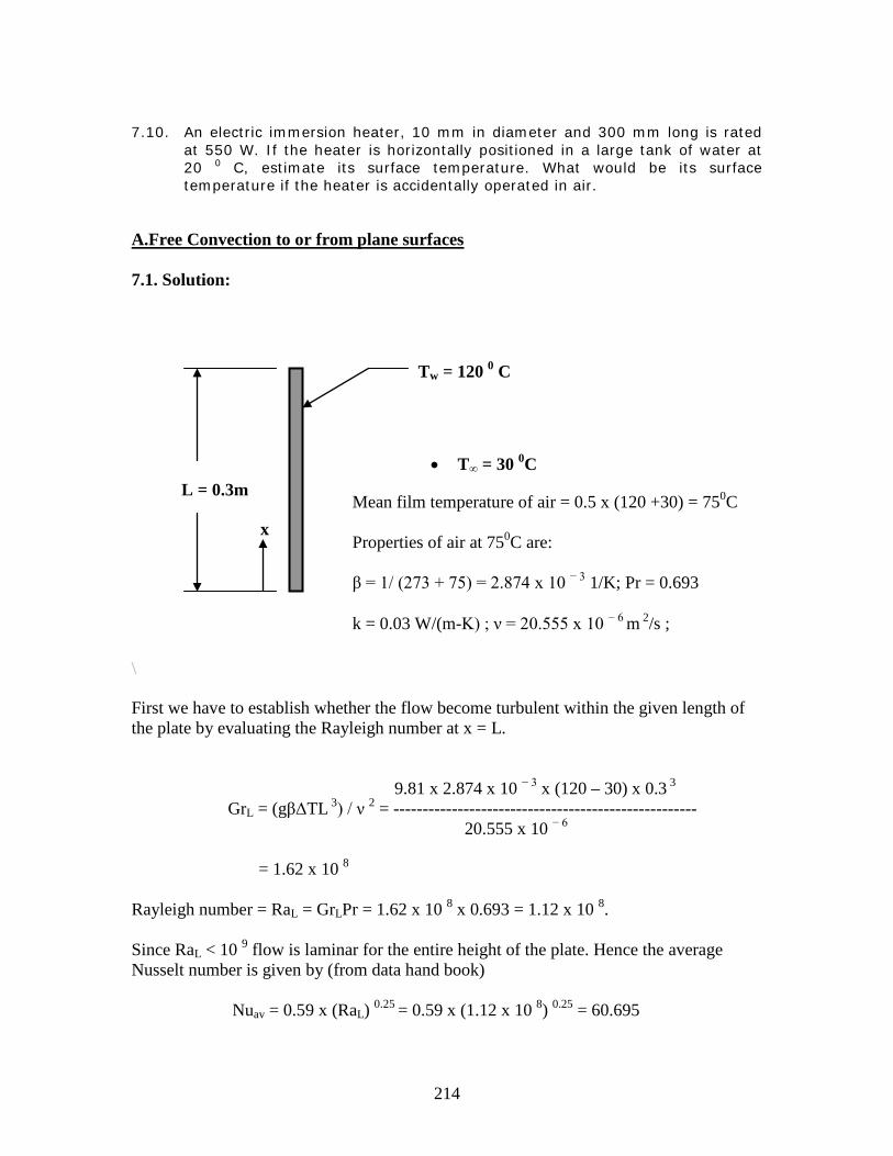
214
7.10. An electric immersion heater, 10 mm in diameter and 300 mm long is rated
at 550 W. If the heater is horizontally positioned in a large tank of water at 20 0 C, estimate its surface temperature. What would be its surface temperature if the heater is accidentally operated in air.
A.Free Convection to or from plane surfaces 7.1. Solution:
\ First we have to establish whether the flow become turbulent within the given length of the plate by evaluating the Rayleigh number at x = L. 9.81 x 2.874 x 10 − 3 x (120 – 30) x 0.3 3 GrL = (gβΔTL 3) / ν 2 = ---------------------------------------------------- 20.555 x 10 − 6 = 1.62 x 10 8 Rayleigh number = RaL = GrLPr = 1.62 x 10 8 x 0.693 = 1.12 x 10 8. Since RaL < 10 9 flow is laminar for the entire height of the plate. Hence the average Nusselt number is given by (from data hand book) Nuav = 0.59 x (RaL) 0.25 = 0.59 x (1.12 x 10 8) 0.25 = 60.695
L = 0.3m
x
Tw = 120 0 C
• T∞ = 30 0C
Mean film temperature of air = 0.5 x (120 +30) = 750C Properties of air at 750C are: β = 1/ (273 + 75) = 2.874 x 10 − 3 1/K; Pr = 0.693 k = 0.03 W/(m-K) ; ν = 20.555 x 10 − 6 m 2/s ;

215
60.6 x 0.03 Therefore hav
= Nuav k / L = ---------------- = 6.069 W /(m2 – K). 0.3
Total heat transfer fro both sides of the plate per unit width of the plate is given by Qtotal = hav(2LW) ΔT = 6.06 x (2 x 0.3 x 1) X (120 – 30) = 327.726 W/m. 7.2. Solution:
Since Tw is not known, it is not possible to determine the mean film temperature at which fluid properties have to be evaluated. Hence this problem requires a trial and error solution either by assuming Tw and then calculate Tw by using the heat balance equation and check for the assumed value or assume a value for hav ,calculate Tw and then calculate hav and check for the assumed value of hav.Since it is difficult to guess a reasonable value for Tw to reduce the number of iterations, it is preferable to guess a reasonable value for hav for air as we know that for air hav varies anywhere between 5 and 15 W/(m2-K). Trial 1:- Assume hav = 10 W/(m2-K). Now qw = hav[Tw – T∞] or Tw = T∞ + qw / hav = 30 + 600 / 10 = 900C. Hence mean film temperature = 0.5 x [90 + 30] = 60 0C. Properties of air at 60 0C are: β = 1 / (60 + 273 ) = 3.003 x 10 − 3 1/K; Pr = 0.696; k = 0.02896 W/(m-K); ν = 18.97 x 10 − 6 m2/s.
Insulated
qw = 600 W/m2
• T∞ = 30 0C
L = 0.25 m

216
9.81 x 3.003 x 10 − 3 x 600 x (0.25)4
RaL* = GrL*Pr =[(gβqwx4) /(kν2)]Pr = ----------------------------------------------x 0.696
0.02896 x (18.97 x 10 − 6) 2 Or RaL
* = 4.61 x 10 9. Since RaL
* >10 9 flow is turbulent for the entire length of the plate Hence Nuav = 1.25 Nux|x=L = 1.25 x 0.17 x (4.61 x 10 9) 0.2 = 55.37 Therefore hav = 55.37 x 0.02896 / 0.25 = 6.41 W/(m2 – K) Since the calculated value of hav deviates from the assumed value by about 34 %, one more iteration is required. Trial 2:- Assume hav = 6.41 W/(m2-K) Hence Tw = 30 + 600 / 6.41 = 123.6 0C ≅120 0 C Mean film temperature = 0.5 x (120 + 30) = 75 0 C Properties of air at 75 0C are:- β = 1/(75 + 273) = 2.873 x 10 − 3 1/K. Pr = 0.686 k = 0.03338 W /(m-K); ν = 25.45 x 10 − 6 m 2 /s. 9.81 x 2.873 x 10 − 3 x 600 x 0.25 4 RaL* = ------------------------------------------- x 0.686 = 2.06 x 10 9 0.03338 x (25.45 x 10 − 6) 2 Flow is turbulent for the entire length of the plate. Hence Nuav = 1.25 Nux|x=L = 1.25 x 0.17 x (2.06 x 10 9) 0.25 = 45.27 Therefore hav = 45.27 x 0.03338 / 0.25 = 6.04 W/(m2 – K). Since the calculated value of hav is very close to the assumed value, the iteration is stopped. The surface temperature of the plate is therefore given by Tw = 30 + 600 / 6.04 = 129.3 0 C. 7.3. Solution:- Case(i) When the plate is vertical Data:- Characteristic length = L = height of the plate = 0.3 m; Tw = 100 0C;T∞= 20 0C; Mean film temperature = 0.5 x (100 + 20) = 60 0C.
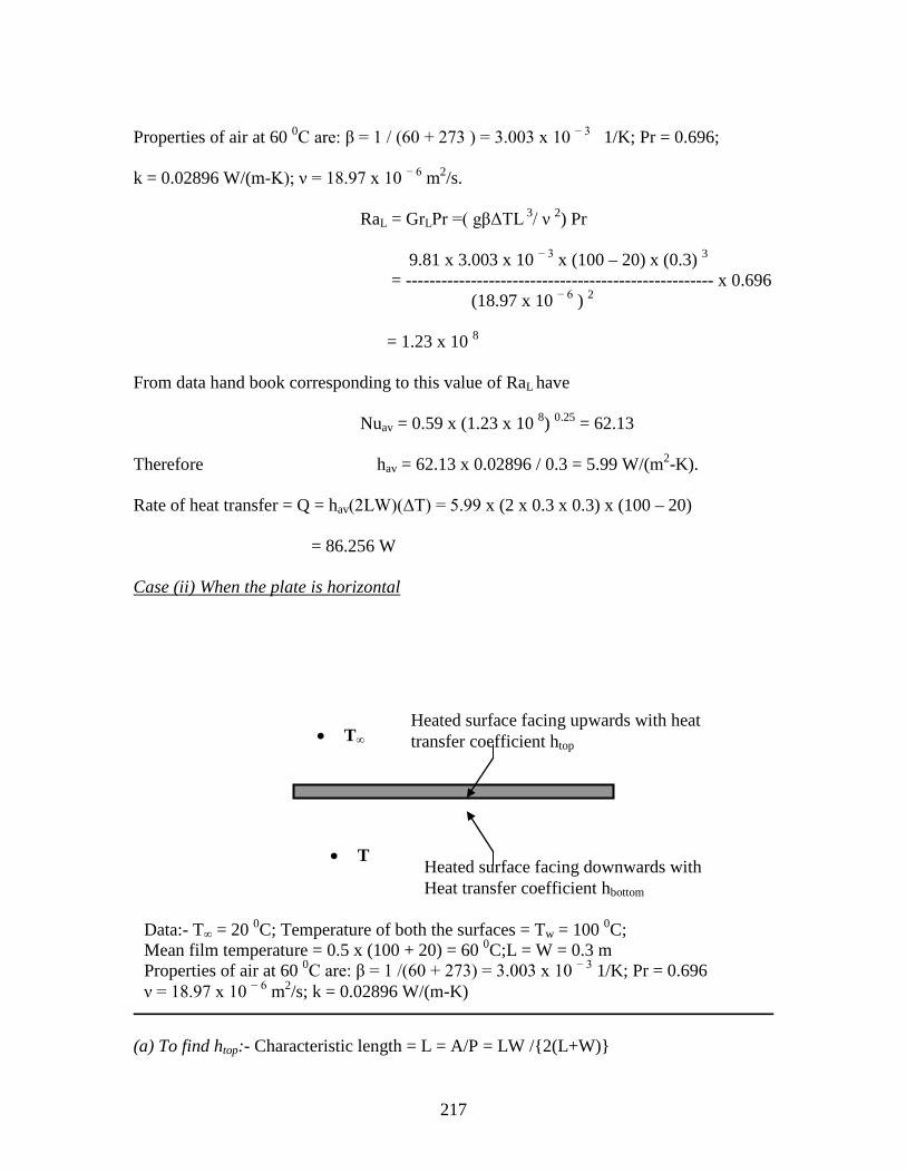
217
Properties of air at 60 0C are: β = 1 / (60 + 273 ) = 3.003 x 10 − 3 1/K; Pr = 0.696; k = 0.02896 W/(m-K); ν = 18.97 x 10 − 6 m2/s. RaL = GrLPr =( gβΔTL 3/ ν 2) Pr 9.81 x 3.003 x 10 − 3 x (100 – 20) x (0.3) 3 = ---------------------------------------------------- x 0.696 (18.97 x 10 − 6 ) 2 = 1.23 x 10 8 From data hand book corresponding to this value of RaL have Nuav = 0.59 x (1.23 x 10 8) 0.25 = 62.13 Therefore hav = 62.13 x 0.02896 / 0.3 = 5.99 W/(m2-K). Rate of heat transfer = Q = hav(2LW)(ΔT) = 5.99 x (2 x 0.3 x 0.3) x (100 – 20) = 86.256 W Case (ii) When the plate is horizontal
(a) To find htop:- Characteristic length = L = A/P = LW /{2(L+W)}
Heated surface facing upwards with heat transfer coefficient htop
Heated surface facing downwards with Heat transfer coefficient hbottom
• T∞
• T
Data:- T∞ = 20 0C; Temperature of both the surfaces = Tw = 100 0C; Mean film temperature = 0.5 x (100 + 20) = 60 0C;L = W = 0.3 m Properties of air at 60 0C are: β = 1 /(60 + 273) = 3.003 x 10 − 3 1/K; Pr = 0.696 ν = 18.97 x 10 − 6 m2/s; k = 0.02896 W/(m-K)
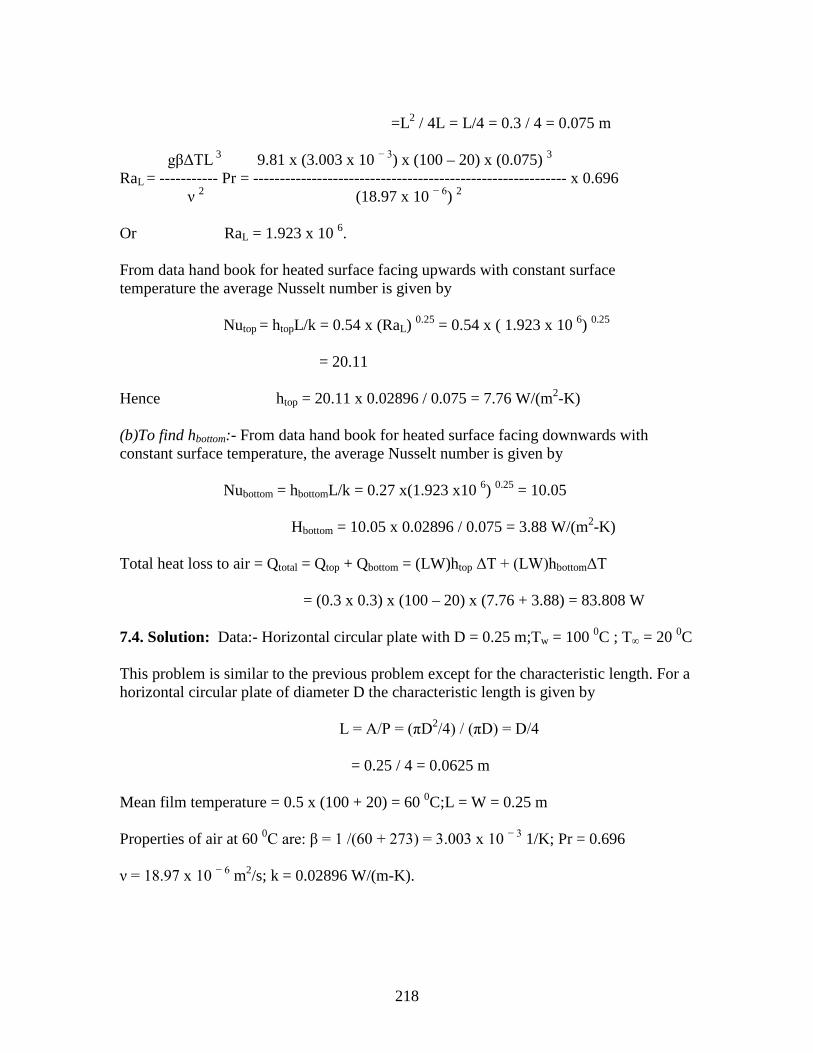
218
=L2 / 4L = L/4 = 0.3 / 4 = 0.075 m gβΔTL 3 9.81 x (3.003 x 10 − 3) x (100 – 20) x (0.075) 3 RaL = ----------- Pr = ----------------------------------------------------------- x 0.696 ν 2 (18.97 x 10 − 6) 2 Or RaL = 1.923 x 10 6. From data hand book for heated surface facing upwards with constant surface temperature the average Nusselt number is given by Nutop = htopL/k = 0.54 x (RaL) 0.25 = 0.54 x ( 1.923 x 10 6) 0.25 = 20.11 Hence htop = 20.11 x 0.02896 / 0.075 = 7.76 W/(m2-K) (b)To find hbottom:- From data hand book for heated surface facing downwards with constant surface temperature, the average Nusselt number is given by Nubottom = hbottomL/k = 0.27 x(1.923 x10 6) 0.25 = 10.05 Hbottom = 10.05 x 0.02896 / 0.075 = 3.88 W/(m2-K) Total heat loss to air = Qtotal = Qtop + Qbottom = (LW)htop ΔT + (LW)hbottomΔT = (0.3 x 0.3) x (100 – 20) x (7.76 + 3.88) = 83.808 W 7.4. Solution: Data:- Horizontal circular plate with D = 0.25 m;Tw = 100 0C ; T∞ = 20 0C This problem is similar to the previous problem except for the characteristic length. For a horizontal circular plate of diameter D the characteristic length is given by L = A/P = (πD2/4) / (πD) = D/4 = 0.25 / 4 = 0.0625 m Mean film temperature = 0.5 x (100 + 20) = 60 0C;L = W = 0.25 m Properties of air at 60 0C are: β = 1 /(60 + 273) = 3.003 x 10 − 3 1/K; Pr = 0.696 ν = 18.97 x 10 − 6 m2/s; k = 0.02896 W/(m-K).

219
gβΔTL 3 9.81 x (3.003 x 10 − 3) x (100 – 20) x (0.0625) 3 RaL = ----------- Pr = ----------------------------------------------------------- x 0.696 ν 2 (18.97 x 10 − 6) 2
Or RaL = 1.112 x 10 6. From data hand book for heated surface facing upwards with constant surface temperature the average Nusselt number is given by Nutop = htopL/k = 0.54 x (RaL) 0.25 = 0.54 x ( 1.112 x 10 6) 0.2 = 17.53 Hence htop = 17.53 x 0.02896 / 0.0625 = 8.12 W/(m2-K) (b)To find hbottom:- From data hand book for heated surface facing downwards with constant surface temperature, the average Nusselt number is given by Nubottom = hbottomL/k = 0.27 x (1.112 x10 6) 0.25 = 8.76 hbottom = 8.76 x 0.02896 / 0.0625 = 4.059 W/(m2-K) Total heat loss to air = Qtotal = Qtop + Qbottom = (πDL)htop ΔT + (πDL)hbottomΔT = (π x 0.25 x 1)x (100 – 20) x (8.76 + 4.059) = 805.44 W 7.5. Soloution: Data:- L = W = 0.25 m; T∞ = 30 0C; Tw = 50 0C; Mean film temperature = 50 − 0.25 x (50 - 30) = 45 0C;Properties of air at 45 0C are: Pr = 0.6835; k = 0.02791 W/(m-K); ν = 17.455 x 10 − 6 m2/s. β = 1/[{30 +0.25x(50-30)} +273] =3.25 x 10 − 3
(i) Inclined plate with heated surface facing upwards:

220
Nuav = 0.145 [RaL
1/3 − (GrcPr)1/3] + 0.56(GrcPrcosθ)1/4 The above correlation is valid only if GrL > Grc. From data hand book for θ = − 50 0, Grc = 4 x 10 8 which is more than GrL.Hence the above correlation cannot be used. Instead the following correlation has to be used. Nuav = 0.59 (GrLcos θ Pr) ¼ = 0.59 x (2.23 x 107 x cos 500) ¼ = 36.3 Hence hav = 36.3 x 0.02791 / 0.25 = 4.05 W/(m2 – K). Therefore Q = 4.05 x (0.25 x 0.25) x (50 – 30) = 5.062 W (ii) Inclined plate with heated surface facing downwards: The correlation for Nusselt number when the heated surface is facing downwards is given by Nuav = 0.56 (GrLcos θ Pr) ¼ = 0.56 x (2.23 x 107 x cos 500) ¼ = 34.45 hav = 34.45 x 0.02791 / 0.25 = 3.84 W/(m2-K). Hence Q = 3.84 x (0.25 x 0.25) x (50 – 30) = 4.8 W 7.6. Solution:
Insulated
θ = − 50 0
Characteristic length = L = 0.25 m gβΔTL3 GrL = ----------- ν 2 9.81 x (50 – 30) x 3.25 x 10−3 x(0.25)3
= ------------------------------------------------- (17.455 x 10 − 6)2 = 3.27 x 10 7 Hence RaL = 3.27 x 10 7 x 0.6835 = 2.23x10⁷
From data hand book, for inclined plate with heated surface facing upwards the Nusselt number is given by

221
9.81 x 2.5 x 10 − 3 x(225 – 20) x 0.2 3 GrL = ---------------------------------------------- = 5.99 x 10 7
(25.9 x 10 − 6) 2 RaL = 5.99 x 10 7 x 0.6865 = 4.11 x 10 7 Hence Nuav = 0.59 x (4.11 x 10 7) 0.25 = 47.24 Therefore hav = 47.24 x 0.03365/0.2 = 7.94 W/(m2-K) 1000 Now Q = havLWΔT or W = Q / (havLΔT) = ----------------------------- 7.94 x 0.2 x (225 – 20) = 3.0718 m 7.7. Solution:
L=0.2 m
W
• T∞=200C
Tw = 225 0 C
Mean film temperature = 0.5 x (225 + 20) = 122.5 0C. Properties of air at 122.50C are: β = 1/(122.5 + 273) = 2.5 x 10 − 3 1/K; ν = 25.90 x 10 − 6 m2/s; Pr = 0.6865; k = 0.03365 W/(m-K).
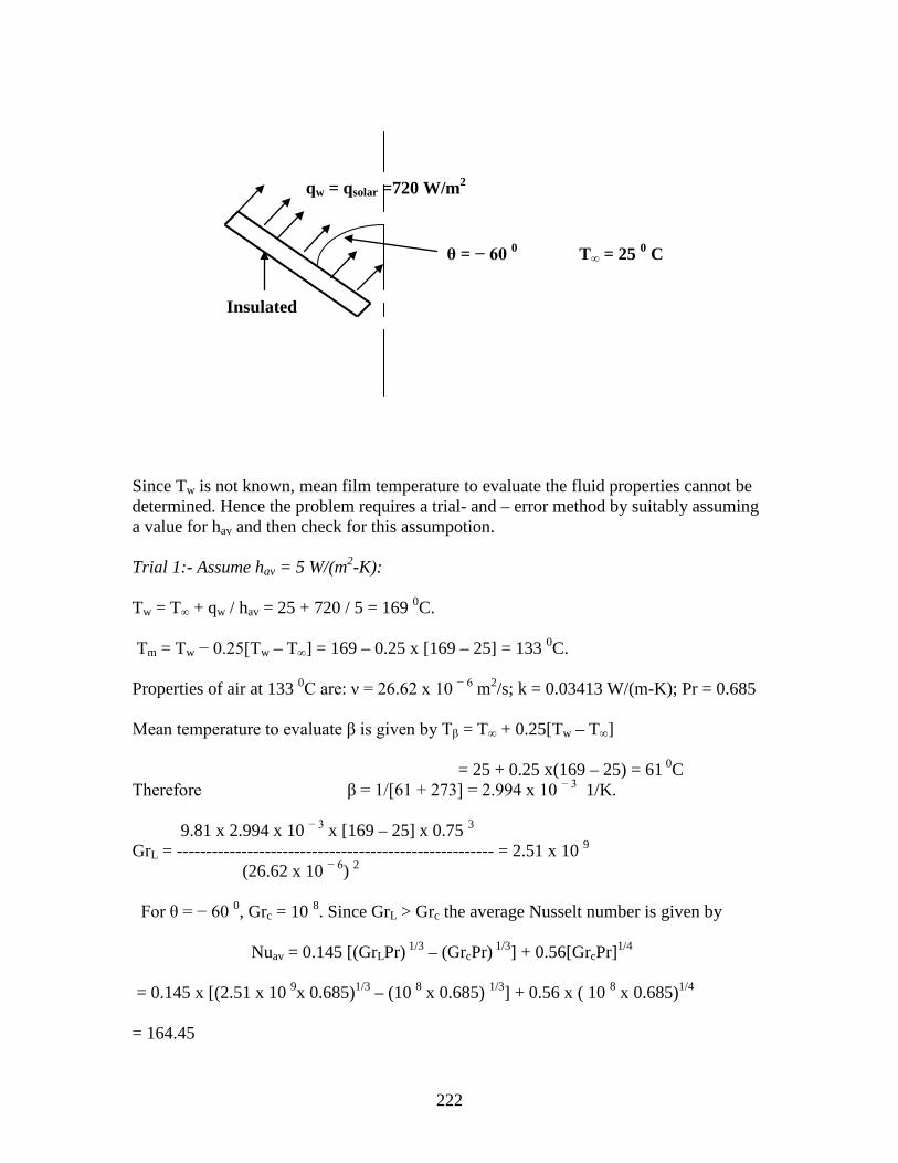
222
Since Tw is not known, mean film temperature to evaluate the fluid properties cannot be determined. Hence the problem requires a trial- and – error method by suitably assuming a value for hav and then check for this assumpotion. Trial 1:- Assume hav = 5 W/(m2-K): Tw = T∞ + qw / hav = 25 + 720 / 5 = 169 0C. Tm = Tw − 0.25[Tw – T∞] = 169 – 0.25 x [169 – 25] = 133 0C. Properties of air at 133 0C are: ν = 26.62 x 10 − 6 m2/s; k = 0.03413 W/(m-K); Pr = 0.685
Mean temperature to evaluate β is given by Tβ = T∞ + 0.25[Tw – T∞] = 25 + 0.25 x(169 – 25) = 61 0C Therefore β = 1/[61 + 273] = 2.994 x 10 − 3 1/K. 9.81 x 2.994 x 10 − 3 x [169 – 25] x 0.75 3
GrL = ------------------------------------------------------ = 2.51 x 10 9
(26.62 x 10 − 6) 2 For θ = − 60 0, Grc = 10 8. Since GrL > Grc the average Nusselt number is given by Nuav = 0.145 [(GrLPr) 1/3 – (GrcPr) 1/3] + 0.56[GrcPr]1/4 = 0.145 x [(2.51 x 10 9x 0.685)1/3 – (10 8 x 0.685) 1/3] + 0.56 x ( 10 8 x 0.685)1/4 = 164.45
Insulated
qw = qsolar =720 W/m2
θ = − 60 0 T∞ = 25 0 C
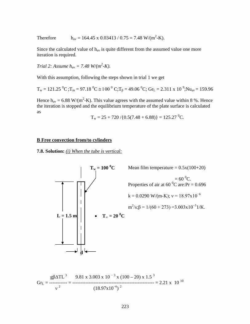
223
Therefore hav = 164.45 x 0.03413 / 0.75 = 7.48 W/(m2-K). Since the calculated value of hav is quite different from the assumed value one more iteration is required. Trial 2: Assume hav = 7.48 W/(m2-K). With this assumption, following the steps shown in trial 1 we get Tw = 121.25 0C ;Tm = 97.18 0C ≅ 100 0 C;Tβ = 49.06 0C; GrL = 2.311 x 10 9;Nuav = 159.96
Hence hav = 6.88 W/(m2-K). This value agrees with the assumed value within 8 %. Hence the iteration is stopped and the equilibrium temperature of the plate surface is calculated as Tw = 25 + 720 /{0.5(7.48 + 6.88)} = 125.27 0C.
B Free convection from/to cylinders 7.8. Solution: (i) When the tube is vertical:
gβΔTL 3 9.81 x 3.003 x 10 − 3 x (100 – 20) x 1.5 3 GrL = ----------- = -------------------------------------------------- = 2.21 x 10 10 ν 2 (18.97x10⁻⁶) 2
L = 1.5 m
d
Tw = 100 0C
• T∞ = 20 0C
Mean film temperature = 0.5x(100+20) = 60 0C. Properties of air at 60 0C are:Pr = 0.696 k = 0.0290 W/(m-K); ν = 18.97x10⁻⁶ m2/s;β = 1/(60 + 273) =3.003x10⁻³¹/K.

224
(L/d) [ 1.5 / 0.05 ] Now ------------ = --------------------------- = 0.0078 GrL
1/4 [2.21 x 10 10] ¼ (L/d) Since ------- < 0.025, the vertical tube/cylinder can be treated as a vertical flat surface GrL
1/4 For calculating the Nusselt number. Now RaL = GrLPr = 2.21 x 10 10 x 0.696 = 1.538 x 10 10
Hence Nuav = 0.1 x (1.538 x 10 10) 1/3 = 248.7 Therefore hav = 248.7 x 0.029 / 1.5 = 4.81 W/(m2 – K). Rate of heat transfer = Q = πdLhavΔT = π x 0.05 x 1.5 x (100 – 20) x 4.81 = 90.67 W (ii) When the pipe is horizontal:- When the pipe is horizontal, the characteristic length is the diameter. Hence gβΔTd 3 9.81 x 3.003 x 10 − 3 x (100 – 20) x 0.05 3 Grd = ----------- = -------------------------------------------------- = 8.185 x 10 5 ν 2 (18.97x10⁻⁶) 2 Rad = 8.185 x 10 5 x 0.696 = 5.697 x 10 5
From data hand book the average Nusselt number is given by 1/6 Rad
[Nuav] ½ = 0.60 + 0.387 ----------------------------------- [1 + (0.559/Pr)9/16] 8/27 1/6 (5.697x 10⁵)
[Nuav] ½ = 0.60 + 0.387 ----------------------------------- = 4.01 or Nuav = 16.08 [1 + (0.559/0.696)9/16] 8/27 Therefore hav = 16.08 x 0.029 / 0.05 = 9.32W/(m2 – K). Q = π x 0.05 x 1.5 x (100 – 20) x 9.32 = 175.67 W 7.9. Solution:
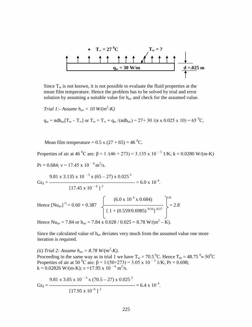
225
Mean film temperature = 0.5 x (27 + 65) = 46 0C. Properties of air at 46 0C are: β = 1 /(46 + 273) = 3.135 x 10 − 3 1/K; k = 0.0280 W/(m-K) Pr = 0.684; ν = 17.45 x 10 − 6 m2/s. 9.81 x 3.135 x 10 − 3 x (65 – 27) x 0.025 3 Grd = ---------------------------------------------------- = 6.0 x 10 4. [17.45 x 10 − 6 ] 2 (6.0 x 10 4 x 0.684) 1/6 Hence [Nuav] ½ = 0.60 + 0.387 ------------------------------------ = 2.8 [ 1 + (0.559/0.6985) 9/16] 8/27 Hence Nuav = 7.84 or hav = 7.84 x 0.028 / 0.025 = 8.78 W/(m2 – K). Since the calculated value of hav deviates very much from the assumed value one more iteration is required. (ii) Trial 2: Assume hav = 8.78 W/(m2-K). Proceeding in the same way as in trial 1 we have Tw = 70.5 0C. Hence Tm = 48.75 0≈ 500C
Properties of air at 50 0C are: β = 1/(50+273) = 3.05 x 10 − 3 1/K; Pr = 0.698; k = 0.02826 W/(m-K); ν =17.95 x 10 − 6 m2/s. 9.81 x 3.05 x 10 − 3 x (70.5 – 27) x 0.025 3 Grd = ---------------------------------------------------- = 6.4 x 10 4. [17.95 x 10⁻⁶ ] 2
Tw = ?
d =.025 m
• T∞ = 27 0C
qw = 30 W/m
Since Tw is not known, it is not possible to evaluate the fluid properties at the mean film temperature. Hence the problem has to be solved by trial and error solution by assuming a suitable value for hav and check for the assumed value. Trial 1:- Assume hav = 10 W/(m2-K) qw = πdhav[Tw – T∞] or Tw = T∞ + qw /(πdhav) = 27+ 30 /(π x 0.025 x 10) = 65 0C.

226
1/6 (6.4 x 104x 0.698)
[Nuav] ½ = 0.60 + 0.387 ----------------------------------- = 2.89 or Nuav = 8.35 [1 + (0.559/0.698)9/16] 8/27 Hence hav = 8.35 x 0.02865 / 0.025 = 9.5691 W/(m2-K). The calculated value of hav agrees with the assumed value within 5 % iteration is stopped. The equilibrium temperature of the surface = Tw = 27 + 30 /(π x 0.025 x 9.5691) = 67 0C. 7.10. Solution:
Case(i):- When the heater is immersed in water For free convection in liquids the order of heat transfer coefficient is around 10 to 1000 W/(m2-K).Let us assume hav = 1000 W/(m2-K). Hence Tw = T∞ + qw / hav = 20 + 58357 / 1000 = 78.4 0C. Mean film temperature = 0.5 x (20 + 78.4) = 49.2 0C. Properties of water at 49.2 0C are: β = 3.103 x 10 − 3 1 / K; Pr = 3.68; k = 0.639 W/(m-K) ; ν = 0.5675 x 10 − 6 m2/s;
d L
Qw
Data:- L = 0.3 m; d = 0.01 m; Qw = 550 W; T∞ = 20 0C; 550 Wall heat flux = qw = Qw /(πdL) = ---------------------- = 58357 W/m2
(π x 0.01 x 0.3) Since Tw is not known, fluid properties cannot be evaluated at the mean temperature and hence the problem has to be solved by trial and error procedure by assuming a suitable value for hav and then check for the assumed value.

227
9.81 x 3.103 x 10 − 3 x (78.4 – 20) x (0.01) 3
Grd = ------------------------------------------------------- = 5.519 x 10 6
(0.5675 x 10 − 6) 2 Rad = 5.519 x 10 6 x 3.68 = 2.03 x 10 7. For horizontal cylinders Nusselt number is given by Nud = C Rad n with C = 0.125 and n = 1/3 for this value of Rad. Hence Nud = 0.125 x (2.03 x 10 7) 1/3 = 33.908 Hence hav = 33.908 x 0.639 / 0.01 = 2166.21 W/(m2 –K) Trial 2:- Assume hav = 2166.21 W/(m2-K) Tw = 20 + 58357 / 2166.21 = 46.940C. Hence mean film temperature =0.5x(20 + 46.94) = 33.47 0C. Properties of water at 33 0C ≈ 300C are : k = 0.6129 W/(m-K); Pr = 5.68; β = 3.3 x 10 − 3; ν = 0.831 x 10 − 6 m2 /s. 9.81 x 3.3 x 10 − 3 x (46.94 – 20) x (0.01) 3
Grd = ----------------------------------------------------- = 2.2 x 10⁶. (0.831 x 10 − 6) 2 Rad = 2.2 x 106 x 5.68 = 1.24 x 10 7 Hence, Nuav = 0.125 x (1.24 x 10 7) 0.333 = 28.77 Therefore, hav = 28.77 x 0.6129 / 0.01 = 1763.3 W/(m2 – K) Trial 3:- Assume hav =1763 W/(m2-K) Tw = 20 + 58357 / 1763 = 53.1 0C. Mean film temperature = 0.5 x (20 + 53.1) = 36.55 0C. Properties of water at 400C are: k = 0.6280 W/(m-K); Pr = 4.34; β = 3.19 x 10 −3 1/K; ν = 0.657 x 10 − 6 m2/s. 9.81 x 3.19 x 10 − 3 x (53 – 20) x (0.01) 3
Rad = ------------------------------------------------- x 4.34 = 1.03 x 10 7 (0.657 x 10 − 6) 2 Hence, Nuav = 0.125 x (1.03 x 10 7) 0.333 = 27.05 Therefore, hav = 27.05x 0.6280 x / 0.01 = 1698.74 W/(m2-K) Since the calculated value of hav agrees with the assumed value within 4%, iteration is stopped and the equilibrium temperature of the heater is calculated as
228
Tw = 20 + 58357 / 1698.74 = 54.35 0C Case (ii):- When the heater is exposed to air When a heated surface is exposed to air the order of heat transfer coefficient varies between 5 and 20 W/(m2-K). Trial 1:- Assume hav = 20 W/(m2-K) Tw = 20 + 58357 / 20 = 2938 0C. Mean film temperature = 0.5 x (20 + 2938) = 1479 0C Properties of air at 1479 0C are : β = 1/(1479 +273) = 5.71 x 10 − 4 1/K; Pr = 0.7045; k = 0.108 W/(m-K); ν = 294.3 x 10 − 6 m2/s. 9.81 x 5.71 x 10 − 4 x (2938 – 20) x (0.01) 3 Rad = ------------------------------------------------- --- x 0.7045 = 133 (294.3 x 10 − 6) 2 Nuav = 0.850 x (133) 0.188 = 2.13 Hence hav = 2.13 x 0.108 / 0.01 = 23 W/(m2-K) This is 13% away from the assumed value and hence one more iteration is required. Trial2:- Assume hav = 23 W/(m2-K) Tw = 20 + 58357 / 23 = 2557 0C ; Mean film temperature = 0.5 x ( 20 + 2557) = 1289 0C Properties of air at 1289 0C are: β = 6.4 x 10 − 4 1/K; ν = 244.34 x 10 − 6 m2/s;Pr = 0.705; k = 0.0978 W/(m-K) 9.81 x 6.4 x 10 − 4 x (2557 – 20) x (0.01) 3 Rad = ------------------------------------------------- --- x 0.705 = 188 (244.34 x 10 − 6) 2 Nuav = 0.850 x (188) 0.188 = 2.275.Hence hav = 2.275 x 0.0978 / 0.01 = 22.25 W/(m2 – K). This value of hav agrees with the assumed value within 4% and hence the iteration is stopped. The equilibrium temperature of the heater is therefore given by Tw = 20 + 58357 / 22.25 = 2643 0C.

229
Chapter 8 : Condensation & Boiling
8.1. Introduction: Knowledge of heat transfer occurring during change of phase i.e. during condensation and boiling is very useful in a number of ways. For example in all power and refrigeration cycles, it is necessary to convert a liquid into a vapour and vice-versa. This is accomplished in boilers or evaporators and condensers. Heat transfer coefficients in both condensation and boiling are generally much higher than those encountered in single phase processes. Values greater than 1000 W/(m2-K) are almost always obtained. This fact has been used in several recent applications where it is desired to transfer high heat fluxes with modest temperature differences. An example is the “heat pipe” which is a device capable of transferring a large quantity of heat with very small temperature differences. 8.2. Film-wise and Drop-wise condensation:- Condensation occurs whenever a vapour comes into contact with a surface at a temperature lower than the saturation temperature of the vapour corresponding to its vapour pressure. The nature of condensation depends on whether the liquid thus formed wets the solid surface or does not wet the surface. If the liquid wets the surface, the condensate flows on the surface in the form of a film and the process is called “film-wise condensation”. If on the other hand, the liquid does not wet the surface, the condensate collects in the form of droplets, which either grow in size or coalesce with neighboring droplets and eventually roll of the surface under the influence of gravity. This type of condensation is called “drop-wise condensation”. The rate of heat transfer during the two types of condensation processes is quite different. For the same temperature difference between the vapour and the surface, the heat transfer rates in drop-wise condensation are significantly higher than those in film-wise condensation. Therefore it is preferable to have drop-wise condensation from the designer’s point of view if the thermal resistance on the condensing side is a significant part of the total thermal resistance. However it is generally observed that, although drop-wise condensation may be obtained on new surfaces, it is difficult to maintain drop-wise condensation continuously and prolonged condensation results in a change to film-wise condensation. Therefore it is still the practice to design condensers under the conservative assumption that the condensation is of film type. 8.3. Nusselt’s theory for laminar film-wise condensation on a plane vertical surface:- The problem of laminar film-wise condensation on a plane vertical surface was first analytically solved by Nusselt in 1916.He made the following simplifying assumptions in his analysis. (i) The fluid properties are constant. (ii) The plane surface is maintained at a uniform temperature, Tw which is less than the saturation temperature Tv of the vapour.

230
8.2 (iii) The vapour is stationary or has a very low velocity and so it does not exert any drag on the motion of the condensate: i.e., the shear stress at the liquid-vapour interface is zero. (iv) The flow velocity of the condensate layer is so low that the acceleration of the condensate is negligible. (v) The downward flow of the condensate under the action of gravity is laminar. (vi) Heat transfer across the condensate layer is purely by conduction; hence the liquid temperature distribution is linear.
Fig. 8.1 : Laminar film condensation on a vertical plate Consider the film-wise condensation on a vertical plate as illustrated in Fig.8.1. Here ‘x’ is the coordinate measured downwards along the plate, and ‘y’ is the coordinate measured normal to the plate from the plate surface. The condensate thickness at any x is represented by δ [ δ = δ(x)]. The velocity distribution u(y) at any location x can be determined by making a force balance on a condensate element of dimensions dx and dy in x and y directions as shown in Fig. 8.1(a). Since it is assumed that there is no acceleration of the liquid in x direction, Newton’s second law in x direction gives ρLdxdyg + pdy + [τ + (∂τ/∂y)dy]dx −τdx − (p + dp)dy = 0 or (∂τ/∂y) = (dp/dx) −ρLg …………………………………..(8.1) Expression for (dp/dx) in terms of vapour density ρv can be obtained by making a force
x
dx
δ
pdy
(p+dp)dy
ρLdxdyg
pdy
(p+dp)dy
ρvdxdyg
y
τdx [τ + (∂τ/∂y)dy]dx
(a) Force balance on a condensate (b) Force balance on a vapour element element at the same distance x from top

231
8.3
balance for a vapour element as shown in Fig. 8.1(b). The force balance gives ρvdxdyg + pdy = (p + dp) dy or (dp/dx) = ρvg Substituting this expression for dp/dx in Eq. (8.1) we have (∂τ/∂y) = (ρv−ρL)g Since the flow is assumed to be laminar, τ = μL(∂u/∂y) Therefore ∂/∂y{μL (∂u/∂y)} = (ρv−ρL)g Integrating with respect to y we have μL (∂u/∂y) = (ρv−ρL)g y + C1 (ρv−ρL)g y C1 Or (∂u/∂y) = --------------- + ------- ……(8.2) μL μL Integrating once again with respect to y we get (ρv−ρL)g y2 C1 y u(y) = ---------------- + ------------- + C2 ......(8.3) 2 μL μL The boundary conditions for the condensate layer are: (i) at y = 0, u = 0; (ii) at y = δ, (∂u/∂y) = 0. Condition (i) in Eq. (8.3) gives C2 = 0 and condition (ii) in Eq. (8.2) gives (ρv−ρL)g δ C1 0 = ------------- + --------- 2 μL μL (ρv−ρL)g δ Therefore C1 = − -------------- 2 Substituting for C1 and C2 in Eq.(8.3) we get the velocity distribution in the condensate layer as

232
8.4 g(ρL − ρv) u(y) = --------------- [ δy – (y2/2)] …………………(8.4) μL If ‘m’ is the mass flow rate of the condensate at any x then δ m = ∫ρLudy 0 δ m = ∫ ρL{ g(ρL − ρv) / μL}[ δy – (y2/2)]dy 0 g ρL (ρL − ρv) δ 3
= ------------------ ………………………………..(8.5) 3 μL g ρL (ρL − ρv) δ 2 dδ Hence dm = ---------------------- μL Amount of heat transfer across the condensate element = dq = dm hfg g ρL (ρL − ρv) δ 2 dδ hfg Or dq = ------------------------- ………………………….(8.6) μL Energy balance for the condensate element shown in the figure can be written as dq = kL(Tv – Tw)dx / δ g ρL (ρL − ρv) δ 2 dδ hfg Or ------------------------- = kL(Tv – Tw)dx / δ………….(8.6) μL kL μL (Tv – Tw)dx or δ 3dδ = ---------------------- g ρL (ρL − ρv) hfg Integrating we get

233
8.5
δ 4 kL μL (Tv – Tw)x ----- = --------------------- + C 3
4 g ρL (ρL − ρv) hfg At x = 0, δ = 0. Hence C3 = 0. Therefore δ 4 kL μL (Tv – Tw)x ----- = ---------------------
4 g ρL (ρL − ρv) hfg 4 kL μL (Tv – Tw)x or δ = [-------------------------- ] 1/ 4……………………(8.7) g ρL (ρL − ρv) hfg Now kL (Tv – Tw)dx ----------------- = hx dx [Tv – Tw] δ kL g ρL (ρL − ρv) hfg kL
3
Therefore hx = --------- = [ --------------------------] 1 / 4
δ 4 μL (Tv – Tw)x g ρL (ρL − ρv) hfg kL
3
Or hx = 0.707[ --------------------------] 1 / 4 ...............................(8.8) μL (Tv – Tw)x The local Nusselt number Nux can therefore be written as hxx g ρL (ρL − ρv) hfg x3
Nux = ----- = 0.707[ --------------------------] 1 / 4 ...............................(8.8) kL μL (Tv – Tw)kL The average heat transfer coefficient for a length L of the plate is given by L hav = (1/L) ∫ hxdx ………………………………………(8.9) 0 It can be seen from Eq. (8.8) that hx = C x − ¼ , where C is a constant given by g ρL (ρL − ρv) hfg kL
3
Or C = 0.707[ --------------------------] 1 / 4 …………………(8.10) μL (Tv – Tw)

234
8.6 L Hence hav = (1/L) C ∫ x − ¼ dx = (C / L) (4/3) L− ¼ = (4/3)C L− ¼ 0 Substituting for C from Eq. (8.10) we have g ρL (ρL − ρv) hfg kL
3
hav = 0.943[ --------------------------] 1 / 4 = (4/3)hx|x = L.........................(8.11) μL (Tv – Tw)L 8.4. Condensation on Inclined Surfaces : Nusselt,s analysis given above can readily be extended to inclined plane surfaces making an angle θ with the horizontal plane as shown in Fig. 8.2.
g sin θρL (ρL − ρv) hfg kL
3
and hav = 0.943[ ----------------------------------] 1 / 4 = (4/3)hx|x = L μL (Tv – Tw)L …………………………(8.13) 8.5. Condensation on a horizontal tube: The analysis of heat transfer for condensation on the outside surface of a horizontal tube is more complicated than that for a vertical
θ
y
g
Fig. 8.2 : Condensation on an inclined plane surface
The component of the gravitational force along the length of the pate is g sin θ.The expressions for local and average heat transfer coefficients can therefore be written as g sin θρL (ρL − ρv) hfg kL
3 hx = 0.707[ ------------------------------------] 1 / 4
μL (Tv – Tw)x …………….......(8.12)
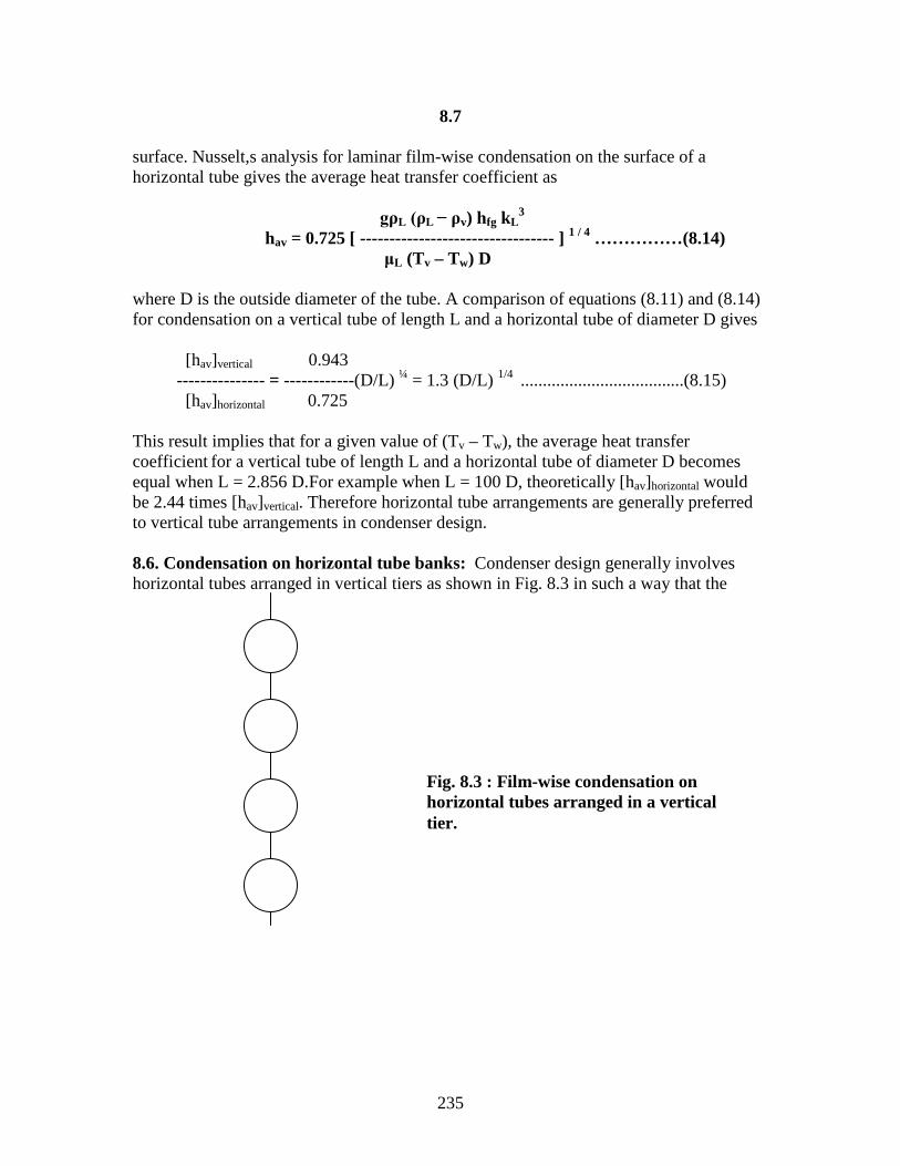
235
8.7 surface. Nusselt,s analysis for laminar film-wise condensation on the surface of a horizontal tube gives the average heat transfer coefficient as gρL (ρL − ρv) hfg kL
3
hav = 0.725 [ --------------------------------- ] 1 / 4 ……………(8.14) μL (Tv – Tw) D where D is the outside diameter of the tube. A comparison of equations (8.11) and (8.14) for condensation on a vertical tube of length L and a horizontal tube of diameter D gives [hav]vertical 0.943 --------------- = ------------(D/L) ¼ = 1.3 (D/L) 1/4 .....................................(8.15) [hav]horizontal 0.725 This result implies that for a given value of (Tv – Tw), the average heat transfer coefficient for a vertical tube of length L and a horizontal tube of diameter D becomes equal when L = 2.856 D.For example when L = 100 D, theoretically [hav]horizontal would be 2.44 times [hav]vertical. Therefore horizontal tube arrangements are generally preferred to vertical tube arrangements in condenser design. 8.6. Condensation on horizontal tube banks: Condenser design generally involves horizontal tubes arranged in vertical tiers as shown in Fig. 8.3 in such a way that the
Fig. 8.3 : Film-wise condensation on horizontal tubes arranged in a vertical tier.

236
8.8 condensate from one tube drains on to tube just below. If it is assumed that the drainage from one tube flows smoothly on to the tube below, then for a vertical tier of N tubes each of diameter D, the average heat transfer coefficient for N tubes is given by gρL(ρL – ρv)hfg kL
3 1 [hav]N tubes = 0.725 [ ----------------------- ] ¼ = ------------ [hav] 1 tube ……………(8.16) μL(Tv – Tw) N D N 1/ 4 This relation generally gives a conservative value for the heat transfer coefficient. Since some turbulence and some disturbance of condensate are unavoidable during drainage, the heat transfer coefficient would be more than that given by the above equation. 8.7. Reynolds number for condensate flow: Although the flow hardly changes to turbulent flow during condensation on a single horizontal tube, turbulence may start at the lower portions of a vertical tube. When the turbulence occurs in the condensate film, the average heat transfer coefficient begins to increase with the length of the tube in contrast to its decrease with the length for laminar film condensation. To establish a criterion for transition from laminar to turbulent flow, a “Reynolds number for condensate flow” is defined as follows. ρL uav Dh Re = ----------------- …………………..(8.17) μL where uav is the average velocity of the condensate film and Dh is the hydraulic diameter for the condensate flow given by 4 x (Cross sectional area for condensate flow) 4A Dh = --------------------------------------------- --------- = ------- Wetted Perimeter P 4A ρL uav 4M Therefore Re = -------------------- = ---------------……………..(8.18) P μL P μL where M is mass flow rate of condensate at the lowest part of the condensing surface in kg/s. The wetted perimeter depends on the geometry of the condensing surface and is given as follows. πD …..For vertical tube of outside diameter D ………….(8.19 a) P = 2L …...For horizontal tube of length L …………………(8.19 b) W ….. For vertical or inclined plate of width W………...(8.19 c) Experiments have shown that the transition from laminar to turbulent condensation takes place at a Reynolds number of 1800. The expression for average heat transfer coefficient for a vertical surface [Eq.(8.11)] can be expressed as follows.

237
8.9 g ρL(ρL – ρv) kL
3 hfg hav = 0.943 [ ----------------------------- ] 1 / 4 μL(Tv – Tw) Generally ρL >> ρv. Therefore g ρL
2 kL3 hfg
hav = 0.943 [ ----------------------------- ] 1 / 4 ………………..(8.20) μL(Tv – Tw) The above equation can be arranged in the form hav [νL
2 / (gkL3) ] 1 / 3 = 1.47 Re L
− 1/ 3 ………………………(8.21) The above equation is valid for ReL < 1800. It has been observed experimentally that when the value of the film Reynolds number is greater than 30, there are ripples on the film surface which increase the value of the heat transfer coefficient. Kutateladze has proposed that the value of the local heat transfer coefficient be multiplied by 0.8(RE / 4)0.11 to account for the ripples effect. Using this correction it can be shown that ReL (hav / kL)( νL
2 / g) 1 / 3 = ------------------------ ………………(8.22) [1.08 ReL
1.22 – 5.2] 8.8. Turbulent film condensation: For turbulent condensation on a vertical surface, Kirkbride has proposed the following empirical correlation based on experimental data. hav [νL
2 / (gkL3) ] 1 / 3 = 0.0077 (ReL) 0.4 ……………………(8.23)
In the above correlation the physical properties of the condensate should be evaluated at the arithmetic mean temperature of Tv and Tw. 8.9. Film condensation inside horizontal tubes: In all the correlations mentioned above, it is assumed that the vapour is either stationary or has a negligible velocity. In practical applications such as condensers in refrigeration and air conditioning systems, vapour condenses on the inside surface of the tubes and so has a significant velocity. In such situations the condensation phenomenon is very complicated and a simple analytical treatment is not possible. Consider, for example, the film condensation on the inside surface of a long vertical tube. The upward flow of vapour retards the condensate flow and causes thickening of the condensate layer, which in turn decreases the condensation heat transfer coefficient. Conversely the down ward flow of vapour decreases the thickness of the condensate film and hence increases the heat transfer coefficient.

238
8.10
Chato recommends the following correlation for condensation at low vapour velocities inside horizontal tubes: g ρL(ρL – ρv) kL
3 h*fg hav = 0.555 [ --------------------------- ] 1 / 4 ……………..(8.24 –a) μL(Tv – Tw) D where h*fg = hfg + (3/8)cp,L(Tv – Tw) ………………………….(8.24 –b) This result has been developed for the condensation of refrigerants at low Reynolds number [Rev = (ρvuvD) / μv < 35,000 ; Rev should be evaluated at the inlet conditions.] For higher flow rates, Akers, Deans and Crosser propose the following correlation for the average condensation heat transfer coefficient on the inside surface of a horizontal tube of diameter D: hav D ------ = 0.026 Pr 1 / 3 [ReL + Rev(ρL / ρv) ½ ] 0.8 ………..(8.25) k where ReL = (4ML) / (πDμL) : Rev = (4Mv) / (πDμv) …………………….(8.26) The above equation correlates the experimental data within 50 % for ReL > 5000 and Rev > 20,000. 8.10. Illustrative examples on film wise condensation: Example 8.1: Saturated steam at 1.43 bar condenses on a 1.9 cm OD vertical tube which is 20 cm long. The tube wall is at a uniform temperature of 109 0C . Calculate the average heat transfer coefficient and the thickness of the condensate film at the bottom of the tube. Solution: Data:- Tv = Saturation temperature at 1.43 bar = 110 0 C (from steam tables) Tw = 109 0C ; Characteristic length = L = 0.2 m ; D = 0.019 m ; To find : (i) hav ; (ii) δ(x)|x=L; Mean film temperature of the condensate (water) = 0.5 x (110 + 109) = 109.5 0C. Properties of water at 109.5 0C are: ρL = 951.0 kg/m3; μL = 258.9 x 10 − 6 N-s / m2; k = 0.685 W/(m-K); ν = 0.2714 x 10 − 6 m2/s; hfg = 2230 kJ/kg. Also ρL >>> ρv.

239
8.11
Let us assume that the condensate flow is laminar and later check for this assumption. g ρL
2 kL3 hfg
hav = 0.943 [ ----------------------------- ] 1 / 4
μL(Tv – Tw) L 9.81 x (951)2x (0.685)3 x 2230 x 103
Hence hav = 0.943 x [--------------------------------------------] 1/ 4 258.9 x 10 − 6 x (110 – 109) x 0.2 = 17,653 W / (m2-K)
(ii) hav = (4 / 3)hx|x=L or hx|x=L = ¾ x hav = 0.75 x 17,653 = 13,240 W/(m2-K). Therefore δ(x)|x=L = kL / hx|x=L = 0.685 / 13240 = 5.174 x 10 − 5 m = 0.0517 mm. Check for Laminar flow assumption:- The relation between hav and Reynolds number at the bottom of the tube is given by hav [νL
2 / (gkL3) ] 1 / 3 = 1.47 Re L
− 1/ 3 or ReL = (1.47 / hav)3(gkL3 / νL
2) Hence ReL = (1.47 / 17,653) 3 [9.81 x 0.685 3 / {0.2714 x 10 − 6}2] = 24.72 Since ReL < 1800, our assumption that condensate flow is laminar is correct. Example 8.2:- Saturated steam at 80 0C condenses as a film on a vertical plate 1 m high. The plate is maintained at a uniform temperature of 70 0C. Calculate the average heat transfer coefficient and the rate of condensation. What would be the corresponding values if the effect of ripples is taken into consideration. Solution:Data:- Tv = 80 0C; Tw = 70 0C; Mean film temperature =0.5 x (80 + 70) = 75 0C. Properties of condensate (liquid water) at 75 0C are: ρL = 974.8 kg/m3; kL = 0.672 W /(m-K) ; μL = 381 x 10 − 6 N-s/m2; hfg at 80 0C = 2309 kJ/kg-K; νL = 0.391 x 10 − 6 m2/s.Charecteristic length = L = 1.0 m. Assuming laminar film condensation the average heat transfer coefficient is given by

240
8.12 g ρL
2 kL3 hfg
hav = 0.943 [ ----------------------------- ] 1 / 4
μL(Tv – Tw) 9.81 x (974.8)2 x (0.672)3 x 2309 x 103
= 0.943 x [ ------------------------------------------------] 1/ 4 = 6066.6 W /(m2 – K). 381.6 x 10 − 6 x (80 – 70 ) x 1.0 hav L (Tv – Tw) 6066.6 x 1.0 x (80 – 70) Condensate rate = M = --------------------- = ------------------------------- 0.0263 kg/s. hfg 2309 x 10 3 4M Check for laminar flow assumption :- ReL = --------------, where P = width of the plate for μL P 4 x 0.0263 vertical flat plate. Hence ReL = ------------------------- = 276 381 x 10 − 6
Since ReL < 1800, the condensate flow is laminar. Since ReL > 30, it is clear that the effects of ripples have to be considered. 4M 4 hav L (Tv – Tw) Now ReL = ------------ = ----------------------- μL P μL P hfg ReL μL P hfg Hence hav = ------------------ …………………………………………….(1) 4L(Tv – Tw) When the effects of ripples are considered the relation between ReL and hav is given by Eq.(8.22) as follows: ReL 1.08 ReL
1.22 – 5.2 = ----------------------- Substituting for hav from Eq.(1) we have (hav/kL)(νL
2 /g)1 /3 4L (Tv – Tw) kL (g / νL
2) 1/3
1.08 ReL1.22 – 5.2 = --------------------------------
μL P hfg 4 x 1 x (80 – 70) x 0.672 x {9.81 /( 0.391 x 10 − 6)2}1/3 1.08 ReL
1.22 – 5.2 = ---------------------------------------------------------------------- 381.6 x 10 − 6 x 1.0 x 2309 x 10 3

241
8.13
1.08 ReL
1.22 – 5.2 = 1221.3. Or ReL = 319.4 319.4 x 381.6 x 10 − 6 x 1.0 x 2309 x 10 3
Hence from Eq.(1) we have hav = ---------------------------------------------------- 4 x 1.0 x (80 – 70) = 7036 W /(m2 – K). hav L (Tv – Tw) 7036 x 1.0 x (80 – 70) Hence M = --------------------- = ---------------------------- = 0.03047 kg / s. hfg 2309 x 10 3 [ It can be seen that the ripples on the surface increase the heat transfer coefficient by about 15 %]. Example 8.3:- Air free saturated steam at 65 0C condenses on the surface of a vertical tube of OD 2.5 cm. The tube surface is maintained at a uniform temperature of 35 0C. Calculate the length of the tube required to have a condensate flow rate of 6 x 10 −3kg/s. Solution:Data:- Tv = 65 0C; Tw = 35 0C; D0 = 0.025 m; M = 6 x 10 − 3 kg/s. To find length of the tube, L. Mean film temperature = 0.5 x (65 + 35) = 50 0C.Properties of condensate (liquid water) at 50 0C are: kL = 0.640 W/(m-K); μL = 0.562 x 10 − 3 N-s/m2; ρL = 990 kg/m3; At 65 0C, hfg = 2346 x 10 3 J/(kg-K). 4M 4 x 6 x 10 − 3
Reynolds number = Re = --------------- = ------------------------------- = 544 μL πDo 0.562 x 10 − 3 x π x 0.025 Since Re < 1800 flow is laminar. It is more convenient to use Eq.(8.21) hav [νL
2 / (gkL3) ] 1 / 3 = 1.47 Re L
− 1/ 3 or (gkL
3) 1.47 x (544)− 1/3 x [9.81 x 0.643] 1/3
hav = 1.47 Re L− 1/ 3 [ ---------- ] 1/3 = ----------------------------------------------
νL2 (0.562 x 10 − 3/ 990)2
= 3599 W/(m2 – K)

242
8.14
Heat balance equation gives M hfg = hav πDoL [Tv – Tw] M hfg 6 x 10 − 3 x 2346 x 10 3
Therefore L = ---------------------- = ------------------------------------ hav πDo [Tv – Tw] 3599 x π x 0.025 x (65 – 35) = 1.66 m Example 8.4:- Air free saturated steam at 85 0C condenses on the outer surfaces of 225 horizontal tubes of 1.27 cm OD, arranged in a 15 x 15 array. Tube surfaces are maintained at a uniform temperature of 75 0C. Calculate the total condensate rate per one metre length of the tube. Solution: Data:- Tv = 85 0C; Tw = 75 0C; Do = 0.0127 m; L = 1 m; Number of tubes in vertical tier = N = 15 ; Total number of tubes = n = 225; Mean film temperature = 0.5 x (85 + 75) = 80 0C. Properties of the condensate (liquid water) are: kL = 0.668 W/(m-K); μL = 0.355 x 10 − 3 N-s/m2; ρL= 974 kg/m3; At 85 0C, hfg = 2296 x 10 3 J/(kg-K). For N horizontal tubes arranged in a vertical tier, hav is given by g ρL
2 hfg kL3
hav = 0.725 [ --------------------- ] 1 / 4
μL(Tv – Tw)NDo 0.725 x [9.81 x (974)2 x (0.668)3] 1/4
hav = ------------------------------------------------------ = 7142 W/(m2 – K) [0.355 x 10 − 3 x (85 – 75) x 15 x 0.0127] ¼ Q = hav Atotal (Tv – Tw) = hav n π DoL (Tv – Tw) = 7142 x 225 x π x 0.0127 x 1 x (85 – 75) = 641.14 x 10 3 W Mass flow rate of condensate = M = Q / hfg = 641.14 x 10 3 / 2296 x 10 3 = 0.28 kg/ (s-m) Example 8.5:- Superheated steam at 1.43 bar and 200 0C condenses on a 1.9 cm OD vertical tube which is 20 cm long. The tube wall is maintained at a uniform temperature of 109 0C. Calculate the average heat transfer coefficient and the thickness of the condensate at the bottom of the tube. Assume cp for super heated steam as 2.01 kJ/(kg-K).

243
8.15
Solution: With a superheated vapour, condensation occurs only when the surface temperature is less than the saturation temperature corresponding to the vapour pressure. Therefore for a superheated vapour, the amount of heat to be removed per unit mass to condense it is given by Q / M = hfg + cpv(Tv – Tsat) Where cp is the specific heat of superheated steam and Tsat is the saturation temperature corresponding to the vapour pressure. If it is assumed that the liquid – vapour interphase is at the saturation temperature, then Eq.(8.20 ) still holds good with hfg replaced by hfg + cpv(Tv – Tsat). Hence g ρL
2 kL3 { hfg + cpv(Tv – Tsat)}
hav = 0.943 [ --------------------------------------- ] 1/ 4
μL(Tsat – Tw)L At 1.43 bar, Tsat = 110 0C.Mean film temperature = 0.5 x (110 + 109) = 109.5 0C. Properties of the condensate at 109.5 0C are: kL = 0.685W/(m-K); μL = 0.259 x 10 − 3 N- s/m2; ρL= 951 kg/m3;At 1.43 bar, hfg = 2230 x 10 3 J/(kg-K). 9.81 x (951)2 x (0.685)3x {2230 x 103 + 2010 x (200 – 110)} hav = 0.943 x [ -------------------------------------------------------------------------- ] 1/ 4
0.259 x 10 − 3 x (110 – 109) x 0.2 = 18,000 W /(m2 – K). Hence hx|x=L = (¾) x 18000 = 13,500 W / (m2 – K). δ(x)|x=L = kL / hx|x=L = 0.685 / 13,500 = 5.07 x 10 − 5m Example 8.6:- Air free saturated steam at 70 0C condenses on the outer surface of a 2.5 cm OD vertical tube whose outer surface is maintained at a uniform temperature of 50 0C. What length of the tube would produce turbulent film condensation? Solution: Data:- Tv = 70 0C; Tw = 50 0C; Do = 0.025 m; Vertical tube. To find L such that Re = 1800. Mean film temperature = 0.5 x (70 + 50) = 60 0C. Properties of the condensate (liquid water) are : kL = 0.659W/(m-K); μL = 0.4698 x 10 − 3 N-s/m2; ρL= 983.2 kg/m3;

244
8.16 At 70 0C hfg = 2358 x 10 3 J/(kg-K). Re (μLπDo) 1800 x 0.4698 x 10 − 3 x π x 0.025 Re = 4M / (μLπDo) or M = ------------------- = ---------------------------------------------
4 4 = 0.0166 kg / s. For turbulent flow hav [νL
2 / (gkL3) ] 1 / 3 = 0.0077 (ReL) 0.4
Or hav = 0.0077 (ReL) 0.4[νL
2 / (gkL3) ] − 1 / 3
Hence hav
= 0.0077 x (1800)0.4 x [ (0.4698 x 10 − 3/983.2)2 / (9.81 x 0.6593) ] − 1 / 3 = 3563.4 W / (m2 – K). Heat balance equation is M hfg = hav π DoL (Tv – Tw) M hfg 0.0166 x 2358 x 10 3
Hence L = ----------------------- = ------------------------------------- hav π Do (Tv – Tw) 3563.4 x π x 0.025 x (70 – 50) = 7 m Example 8.7:- Saturated steam at 100 0C condenses on the outer surface of a 2 m long vertical plate. What is the temperature of the plate below which the condensing film at the bottom of the plate will become turbulent? Solution: Data:- Tv = 100 0C; L = 2 m. Since Tw is not known, properties of the condensate at the mean film temperature cannot be determined and therefore the problem has to be solved by trial and error procedure as follows: Trial 1:- The properties of the condensate are read at Tv = 100 0C. The properties are kL = 0.683 W/(m-K); μL = 0.2824 x 10 − 3 N-s/m2; ρL= 958.4 kg/m3; At 100 0C, hfg = 2257 x 10 3 J/kg-K. Since the flow has to become turbulent at the bottom of the plate we have hav = 0.0077 (ReL) 0.4[νL
2 / (gkL3) ] − 1 / 3 with ReL = 1800

245
8.17 9.81 x 0.683 3
Hence hav = 0.0077 x (1800)0.4 x [ ------------------------------ ] 1 / 3
(0.2824 x 10 − 3 / 958.4) 2 = 5098 W / (m2 – K) Now M hfg = hav L W (Tv – Tw) Or Tw = Tv – (M/W)hfg / (hav L). But ReL = 4M / (μLW) or M/W = ReL μL / 4. ReL μL hfg 1800 x 0.2824 x 10 − 3 x 2257 x 10 3 Therefore Tw = Tv − -------------------- = 100 − ---------------------------------------------- 4 hav L 4 x 5098 x 2 = 72 0C Trial 2:- Assume Tw = 72 0C. Mean film temperature = 0.5 x (100 + 72) = 86 0C. Properties of the condensate at 86 0C ; kL = 0.677 W/(m-K); μL = 0.3349 x 10 − 3 N-s/m2; ρL= 968.5kg/m3; At 100 0C, hfg = 2257 x 10 3 J/(kg-K). 9.81 x 0.677 3
Hence hav = 0.0077 x (1800)0.4 x [ ------------------------------ ] 1 / 3
(0.3349 x 10 − 3 / 968.5) 2 = 4541 W /(m2 – K). 1800 x 0.3349 x 10 − 3 x 2257 x 10 3 Therefore Tw = 100 − ----------------------------------------------- = 60 0C 4 x 4541 x 2 Since the calculated value of Tw is quite different from the assumed value, one more iteration is required. Trial 3:- Assuming Tw = 60 0C and proceeding on the same lines as shown in trial 2 we get hav = 4365 W /(m2 – K) and hence Tw = 590C. This value is very close to the value assumed (difference is within 2 % ). The iteration is stopped. Hence Tw = 59 0C. Example 8.8:- Air free saturated steam at 90 0C condenses on the outer surface of a 2.5 cm OD, 6 m long vertical tube, whose outer surface is maintained at a uniform temperature of 60 0C. Calculate the total rate of condensation of steam at the tube surface.

246
8.18 Solution: Data:- Tv = 90 0C; Tw = 30 0C; Do = 0.025 m; L = 6 m. Vertical tube. Mean film temperature = 0.5 x (90 + 60) = 75 0C. Properties of the condensate at 75 0C are: kL = 0.671 W/(m-K); μL = 0.3805 x 10 − 3 N-s/m2; ρL= 974.8 kg/m3; At 90 0C, hfg = 2283 x 10 3 J/(kg-K). We do not know whether the condensate flow is laminar or turbulent. We start the calculations assuming laminar flow and then check for laminar flow condition. For laminar flow g ρL
2 kL3 hfg
hav = 0.943 [ ----------------------------- ] 1 / 4
μL(Tv – Tw) L 9.81 x (974.8)2 x (0.671)3 x 2283 x 10 3 Hence hav = 0.943 x [--------------------------------------------------] 1 / 4
0.3805 x 10 − 3 x (90 – 60) x 6 = 2935.3 W /(m2 – K). For laminar flow hav [νL
2 / (gkL3) ] 1 / 3 = 1.47 Re L
− 1/ 3 Or ReL = (1.47 / hav)3(gkL
3 / νL2)
= (1.47 / 2935.3)3 x [9.81 x 0.6713 x 974.82 / (0.3805 x 10 − 3)2] = 2443 Since ReL > 1800, flow is turbulent. For turbulent flow hav [νL
2 / (gkL3) ] 1 / 3 = 0.0077 (ReL) 0.4
Or hav = 0.0077 (ReL) 0.4 / [νL
2 / (gkL3) ] 1 / 3……….(1)
ReL = 4M / (μLπDo). But Mhfg = havπDoL (Tv – Tw) or M / (πDo) = havL (Tv – Tw) / hfg 4 havL (Tv – Tw) Therefore ReL = ---------------------- hfg μL Substituting this expression for ReL in equation (1) we have

247
8.19 4 havL (Tv – Tw) hav = 0.0077 [------------------------- ] 0.4 [νL
2 / (gkL3) ] − 1 / 3
hfg μL 4 L (Tv – Tw) (hav )0.6 = 0.0077 [------------------------- ] 0.4 [νL
2 / (gkL3) ] − 1 / 3
hfg μL 4 x 6 x (90 – 60) (0.3805 x 10 − 3)2
= 0.0077 x [--------------------------------------- ] 0.4 x [ --------------------------------- ] − 1 / 3
2283 x 10 3 x 0.3805 x 10 − 3 974.82 x 9.81 x (0.671)3 = 192. Hence hav = [192] 1 / 0.6 = 6390 W /(m2 – K). havπDoL (Tv – Tw) 6390 x π x 0.025 x 6 x(90 – 60) Therefore M = ----------------------- = ------------------------------------------ = 0.0396 kg/s hfg 2283 x 10 3 8.11.Dropwise Condensation: Experimental investigations on condensation have indicated that, if traces of oil are present in steam and the condensing surface is highly polished , the condensate film breaks into droplets. This type of condensation is called “drop wise condensation”. The droplets grow, coalesce and run off the surface, leaving a greater portion of the condensing surface exposed to the incoming steam. Since the entire condensing surface is not covered with a continuous layer of liquid film, the heat transfer rate for ideal drop wise condensation is much higher than that for film wise condensation. The heat transfer coefficient may be 2 to 3 times greater for drop wise condensation than for film wise condensation. Hence considerable research has been done with the objective of producing long lasting drop wise condensation. Various types of chemicals have been tried to promote drop wise condensation. Continuous drop wise condensation, obtainable with different promoters varies between 100 to 300 hours with pure steam and are shorter with industrial steam. Failure occurs because of fouling or oxidation of the surface, or by the flow of the condensate or by a combination of these effects. It is unlikely that long lasting drop wise condensation can be produced under practical conditions by a single treatment of any of the promoters currently available. Therefore in the analysis of a heat exchanger involving condensation of steam, it is recommended that film wise condensation be assumed for the condensing surface. 8.12. Boiling Types: When evaporation occurs at a solid-liquid interface, it is called as “boiling”. The boiling process occurs when the temperature of the surface Tw exceeds the saturation temperature Tsat corresponding to the liquid pressure. Heat is transferred from the solid surface to the liquid, and the appropriate form of Newton’s law of cooling is
248
8.20 qw = h [Tw – Tsat] = h ∆Te …………………………(8.27)
Where ∆Te = [Tw - Tsat] and is termed as the “excess temperature”. The boiling process is characterized by the formation of vapour bubbles which grow and subsequently detach from the surface. Vapour bubble growth and dynamics depend, in a complicated manner, on the excess temperature ∆Te, the nature of the surface, and the thermo-physical properties of the fluid, such as its surface tension. In turn the dynamics of vapour bubble growth affect fluid motion near the surface and therefore strongly influence the heat transfer coefficient. Boiling may occur under varying conditions. For example if the liquid is quiescent and if its motion near the surface is due to free convection and due to mixing induced by bubble growth and detachment, then such a boiling process is called “pool boiling”. In contrast in “forced convection boiling”, the fluid motion is induced by an external means as well as by free convection and bubble induced mixing. Boiling may also be classified as “sub-cooled boiling” and “saturated boiling”. In sub-cooled boiling, the temperature of the liquid is below the saturation temperature and the bubbles formed at the surface may condense in the liquid. In contrast, in saturated boiling, the temperature of the liquid slightly exceeds the saturation temeperature, Bubbles formed at the surface are then propelled through the liquid by buoyancy forces, eventually escaping from a free surface. 8.13. Pool Boiling Regimes: The first investigator who established experimentally the different regimes of pool boiling was Nukiyama. He immersed an electric resistance wire into a body of saturated water and initiated boiling on the surface of the wire by passing electric current through it. He determined the heat flux as well as the temperature from the measurements of current and voltage. Since the work of Nukiyama, a number of investigations on pool boiling have been reported. Fig. 8.4 illustrates the characteristics of pool boiling for water at atmospheric pressure. This boiling curve illustrates the variation of heat flux or the heat transfer coefficient as a function of excess temperature ∆Te. This curve pertains to water at 1 atm pressure.From Eq. (8.27) it can seen that qw depends on the heat transfer coefficient h and the excess temperature ∆Te. Free Convection Regime(up to point A):- Free convection is said to exist if ∆Te ≤ 5 0 C. In this regime there is insufficient vapour in contact with the liquid phase to cause boiling at the saturation temperature. As the excess temperature is increased, the bubble inception will eventually occur, but below point A (referred to as onset of nucleate boiling,ONB), fluid motion is primarily due to free convection effects.Therefore,according to whether the flow is laminar or turbulent, the heat transfer coefficient h varies as ∆Te
1/4 or as ∆Te
1/3 respectively so that qw varies as ∆Te5/4 or as ∆Te
4/3. Nucleate Boiling Regime(Between points A and C):- Nucleate boiling exists in the range 5 0 C ≤ ∆Te ≤ 30 0 C. In this range, two different flow regimes may be distinguished. In the region A – B, isolated bubbles form at nucleation sites and separate from the surface, substantially increasing h and qw. In this regime most of the heat exchange is through

249
8.21 direct transfer from the surface to liquid in motion at the surface, and not through vapour bubbles rising from the surface. As ∆Te is increased beyond 10 0C (Region B-C), the nucleation sites will be numerous and the bubble generation rate is so high that continuous columns of vapour appear. As a result very high heat fluxes are obtainable in this region. In practical applications, the nucleate boiling regime is most desirable, because large heat fluxes are obtainable with small temperature differences. In the nucleate boiling regime, the heat increases rapidly with increasing excess temperature
∆Te until the peak heat flux is reached. The location of this peak heat flux is called the burnout point, or departure from nucleate boiling (DNB), or the critical heat flux (CHF). The reason for calling the critical heat flux the burnout point is apparent from the Fig. 8.4. Such high values of ∆Te may cause the burning up or melting away of the heating element. Film Boiling Regime:- It can be seen from Fig. 8.4 that after the peak heat flux is reached, any further increase in ∆Te results in a reduction in heat flux. The reason for this curious phenomenon is the blanketing of the heating surface with a vapour film which restricts liquid flow to the surface and has a low thermal conductivity. This regime is called the film boiling regime. The film boiling regime can be separated into three distinct regions namely (i) the unstable film boiling region, (ii) the stable film boiling region and (iii) radiation dominating region. In the unstable film boiling region, the vapour film is unstable, collapsing and reforming under the influence of convective currents and the
107 106
105 104 103
qw, W/m2
120
1.0 5.0 10 30 100 1000 10000 ∆Te = Tw − Tsat Fig. 8.4: Typical boiling curve for water at 1 atm; surface heat flux qw as function of excess temperature ∆Te

250
8.22 surface tension. Here the heat flux decreases as the surface temperature increases, because the average wetted area of the heater surface decreases. In the stable film boiling region, the heat flux drops to a minimum, because a continuous vapour film covers the heater surface.In the radiation dominating region, the heat flux begins to increase as the excess temperature increases, because the temperature at the heater surface is sufficiently high for thermal radiation effects to augment heat transfer through the vapour film. 8.14. Pool Boiling Correlations: Correlation for The Nucleate Boiling Regime:- The heat transfer in the nucleate boiling regime is affected by the nucleation process, the distribution of active nucleation sites on the surface, and the growth and departure of bubbles.Numerous experimental investigations have been reported and a number of attempts have been made to correlate the experimental data corresponding to nucleate boiling regime.The most successful and widely used correlation was developed by Rohsenow. By analyzing the significance of various parameters in relation to forced - convection effects. He proposed the following empirical relation to correlate the heat flux in the entire nucleate boiling regime: Cpl ∆Te qw _______________ ------------- = Csf [ --------- √ σ* / {g (ρl – ρv)} ] 0.33 ………………. (8.28) hfg Prl
n (μl hfg) where Cpl = specific heat of saturated liquid, J /(kg -0C) Csf = constant to be determined from experimental data depending upon Heating surface – fluid combination hfg = latent heat of vapourization, J / kg g = acceleration due to gravity, m / s2 Prl = Prandtl number of saturated liquid qw = boiling heat flux, W / m2 ∆Te = excess temperature as defined in Eq. (8.27) μl = viscosity of saturated liquid, kg / (m – s) ρl, ρv = density of liquid and saturated vapour respectively, kg / m3 σ* = surface tension of liquid – vapour interface, N / m.

251
8.23 In Eq. (8.28) the exponent n and the coefficient Csf are the two provisions to adjust the correlation for the liquid – surface combination. Table 8-1 gives the experimentally determined values Csf for a variety of liquid – surface combinations. The value of n should be taken as 1 for water and 1.7 for all other liquids shown in Table 8 – 1. Table 8 – 1: Values of Csf of Eq. (8.28) for various liquid – surface combinations Liquid – surface combination Csf
Water – Copper 0.0130 Water – scored copper 0.0068 Water – chemically etched stainless steel 0.0130 Water – mechanically polished stainless steel 0.0130 Water – ground and polished stainless steel 0.0060 Water – brass 0.0060 Water – nickel 0.0060 Water – platinum 0.0130 n-Pentane – polished copper 0.0154 n-Pentane – lapped copper 0.0049 Benzene – chromium 0.1010 Ethyl alcohol – chromium 0.0027 Correlations for Peak Heat Flux:- The correlation given by Eq. (8.28) provides information for the heat flux in nucleate boiling, but it cannot predict the peak heat flux.Based on stability considerations, Kutateladze and Zuber veloped the following correlation to calculate the peak heat flux in pool boiling from an infinite horizontal plate facing up. Π σ* g (ρl – ρv) qmax = ----- ρv hfg [ ---------------------- ] ¼ [ 1 + ρv / ρl ] ½ ………….(8.29)
24 ρv2
where σ * = surface tension of liquid – vapour interface, N / m g = acceleration due to gravity, m / s2 ρl, ρv = density of liquid and vapour respectively, kg / m3 hfg = latent heat of vapourization, J / kg qmax = peak heat flux, W / m2 It is apparent from this equation that large values of hfg, ρv, g and σ * are desirable for a large value of the peak heat flux. For example, water has a large value of hfg; hence the peak heat flux obtainable with boiling water is high. This equation also shows that a reduced gravitational field decreases the peak heat flux. For most situations, the quantity [ 1 + ρv / ρl ] ½ is approximately equal to unity. Hence Eq. (8.29) can be written as
252
8.24
π qmax = ----- ρv
1/2 hfg [σ* g (ρl – ρv) ] ¼ ………………………..(8.30)
24 Lienhard and Dhir improved the analysis and considered the effect of the size of the horizontal plate. They showed that qmax = 0.149 hfg ρv
1/2 [σ* g (ρl – ρv) ] ¼ ……………………….(8.31) The above expression was shown to be valid as long as the plate is large and the dimensionless quantity L [g (ρl – ρv) / σ* ] ½ ≥ 2.7, where L is the characteristic dimension of the plate. For circular plate L is taken as the diameter, while for a square plate it is taken as the side of the plate. For the case of horizontal cylinders of radius R, Lienhard & Sun recommended the following modified form of Eq. (8.30). π qmax = ----- ρv
1/2 hfg [σ* g (ρl – ρv) ] ¼ f(L’) ……………………..(8.32)
24 where f(L’) = 0.89 + 2.27 exp { − 3.44 √L’ }, and L’ = R [g (ρl – ρv) / σ* ] ½. Eq. (8.32) is valid for situations in which L’ ≥ 0.15. This equation cal also be used for large spheres in which case f(L’) = 0.84 and L’ = 4.26. For small spheres f(L’) = 1.734 / √L’, where 0.15 ≤ L’ ≤ 4.26. Correlations for Film boiling Regime:- No satisfactory correlation exists for the unstable film boiling region. For the stable film boiling region, Bromley has derived the following correlation for horizontal cylinders: kv
3 ρv (ρl – ρv) g hfg*
ho = 0.62 [ ----------------------------------- ] ¼ ……………………………………(8.33) D μv ∆Te Where ho = average boiling heat transfer coefficient in the absence of radiation W/(m2 –K), D = outside diameter of the tube, hfg
* = Difference between the enthalpy of the vapour at the mean film temperature,Tm (Tm = [Tw + Tsat] / 2) and the enthalpy of the liquid at the saturation temperature ≈ hfg
+ 0.8 Cpv ∆Te.

253
8.25
In the above correlation, all the vapour properties are evaluated at the mean film temperature while the liquid density is evaluated at the saturation temperature. Since radiation is significant in film boiling, the radiation component has to be added in order to obtain the total heat transfer. Brmoley has shown that the total heat transfer coefficient h is given by the relation h = ho [ho / h ] 1/3 + hr …………………………….(8.34) where hr is the radiation heat transfer coefficient which is calculated from the formula for the radiation heat exchange between parallel planes; 1 σ [ Tw
4 – Tsat4 ]
hr = ----------------------- ------------------------- ……(8.35) [ 1 / ε + 1 / α – 1] [Tw – Tsat where α = absorptivity of liquid and ε = emissivity of the hot tube . Eq.(8.34) is difficult to use because a trial and error approach is needed to determine h. When hr is smaller than ho, Eq. (8.34) can be replaced by h = ho + ¾ hr ………………………………………(8.36) 8.15. Illustrative examples on pool boiling Example 8.9:- Saturated water at 100 0C is boiled with a copper heating element having a heating surface area of 0.04 m2which is maintained at a uniform temperature of 115 0C. Calculate the surface heat flux and the rate of evaporation of water. Also calculate the critical flux. Solution: Given:- Tsat = 100 0C; Tw = 115 0C; Surface area = A = 0.04 m2; Properties of liquid water at 100 0C are: Cpl = 4216 J/(kg – K); hfg = 2257 x 10 3 J/kg; ρl = 960.6 kg/m3; ρv = 0.5977 kg/m3; Prl = 1.75; μl = 282.4 x 10 − 6 kg/(m – s); σ* = 58.8 x 10 − 3 N/m ; ∆Te = 115 – 100 = 15 0C. Since ∆Te lies between 5 0C and 30 0C, the boiling is in the nucleate regime. Csf = 0.0130 for water – copper combination and for water n = 1.For nucleate boiling region we can use Eq. (8.28) which is as follows:
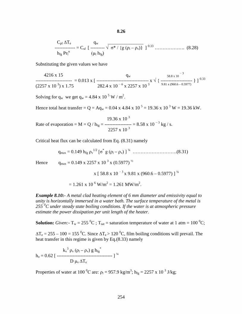
254
8.26
Cpl ∆Te qw _______________ ------------- = Csf [ --------- √ σ* / {g (ρl – ρv)} ] 0.33 ………………. (8.28) hfg Prl
n (μl hfg) Substituting the given values we have 4216 x 15 qw 58.8 x 10
− 3 ----------------------- = 0.013 x [ --------------------------------- x √ { -------------------- } ] 0.33
(2257 x 10 3) x 1.75 282.4 x 10 − 6 x 2257 x 10 3 9.81 x (960.6 – 0.5977)
Solving for qw we get qw = 4.84 x 10 5 W / m2. Hence total heat transfer = Q = Aqw = 0.04 x 4.84 x 10 5 = 19.36 x 10 3 W = 19.36 kW. 19.36 x 10 3
Rate of evaporation = M = Q / hfg = ----------------- = 8.58 x 10 − 3 kg / s. 2257 x 10 3 Critical heat flux can be calculated from Eq. (8.31) namely qmax = 0.149 hfg ρv
1/2 [σ* g (ρl – ρv) ] ¼ ……………………….(8.31) Hence qmax = 0.149 x 2257 x 10 3 x (0.5977) ½ x [ 58.8 x 10 − 3 x 9.81 x (960.6 – 0.5977) ] ¼ = 1.261 x 10 6 W/m2 = 1.261 MW/m2. Example 8.10:- A metal clad heating element of 6 mm diameter and emissivity equal to unity is horizontally immersed in a water bath. The surface temperature of the metal is 255 0C under steady state boiling conditions. If the water is at atmospheric pressure estimate the power dissipation per unit length of the heater. Solution: Given:- Tw = 255 0C ; Tsat = saturation temperature of water at 1 atm = 100 0C; ∆Te = 255 – 100 = 155 0C. Since ∆Te > 120 0C, film boiling conditions will prevail. The heat transfer in this regime is given by Eq.(8.33) namely kv
3 ρv (ρl – ρv) g hfg*
ho = 0.62 [ ----------------------------------- ] ¼ D μv ∆Te
Properties of water at 100 0C are: ρl = 957.9 kg/m3; hfg = 2257 x 10 3 J/kg;

255
8.27
ρv = 4.808 kg/m3; Cpv = 2.56 x 10 3 J/(kg-K); kv = 0.0331 W / (m-0C); μv = 14.85 x 10 − 6 kg / (m-s). Substituting these values in the expression for ho we have (0.0331)
3x 4.808 x (957.9 – 4.808) x 9.81 x {2257 x 10
3 + 0.8 x 2.56 x 10 3
x 155 } ho = 0.62 x [---------------------------------------------------------------------- ] ¼
14.85 x 10 − 6 x 0.006 x 155 = 460 W/(m2 – K) 1 σ {Tw
4 – Tsat4}
hr = ---------------------- x ------------------------------ [1/ε + 1/α − 1 ] {Tw – Tsat} 1 5.67 x 10 − 8 x { 528 4 – 373 4} = ------------------------ x ------------------------------------------- [ 1 / 1 + 1 / 1 − 1 ] { 528 – 373} = 21.3 W / (m2-K). Now h ≈ ho + ¾ hr = 460 + ¾ x 21.3 = 476 W /(m2 – K). Hence Q = h A ∆Te = 476 x (π x 0.006 x 1)x 155 = 1.36 x 10 3 W / m. Example 8.11:- A vessel with a flat bottom and 0.1 m2 in area is used for boiling water at atmospheric pressure. Find the temperature at which the vessel must be maintained if a boiling rate of 80 kg/h is desired. Assume that the vessel is made of copper and the boiling is nucleate boiling. Take ρv = 0.60 kg/m3. Solution: Given:- A = 0.1 m2; Tsat = 100 0C; M = 80 kg/h = 0.022 kg/s; Prl = 1.75 hfg = 2257 x10 3 J /kg; Cpl = 4216 J/(kg-K); ρl = 960.6 kg/m3; σ* = 58.8 x 10 − 3 N/m; μl = 282.4 x 10 − 6 kg / (m-s); n = 1; For water-copper combination Csf = 0.0130; M hfg 0.022 x 2257 x 10 3
qw = Q / A = -------- = ---------------------------- = 4.965 x 10 3 W/m2
A 0.1 For nucleate boiling Eq.(8.28) is used to calculate the excess temperature .∆Te

256
8.28
Cpl ∆Te qw _______________ ------------- = Csf [ --------- √ σ* / {g (ρl – ρv)} ] 0.33 hfg Prl
n (μl hfg) 4216 x ∆Te ----------------------- = 0.013 x {4.965 x 10 5/(282.4 x 10− 6x 2257 x 103) 2257 x 10 3 x 1.75 _____________________________ x √ 58.8 x 10 − 3 / [9.81 x (960.6 – 0.6)] } 0.33 Or ∆Te = 15.2 0C Hence Tw = 100 + 15.2 = 115.2 0C. Example 8.12:- Calculate the heat transfer coefficient during stable film boiling of water from a 0.9 cm diameter horizontal carbon tube. The water is saturated and at 100 0C and the tube surface is at 1000 0C. Take the emissivity of the carbon surface to be 0.8 and assume that at the average film temperature, the steam has the following properties. kv = 0.0616 W/(m-K); ρv = 0.266 kg/m3; μv = 28.7 x 10 −6 kg/(m-s); Cpv = 2168 J/(kg-K); ρl = 958.4 kg/m3
Solution: Given:- D = 0.009 m; ∆Te = Tw – Tsat = 1000 – 100 = 900 0C; ε = 0.8; α = 1.0 hfg
* = hfg + 0.8 Cpv ∆Te = 2257 x 10 3 + 0.8 x 2168 x 900 = 3818 x 10 3 J/kg. For stable film boiling the convection coefficient is given by Eq.(8.33) kv
3 ρv (ρl – ρv) g hfg*
ho = 0.62 [ ----------------------------------- ] ¼ D μv ∆Te
(0.0616)3 x 0.266 x (958.4 – 0.266) x 9.81 x 3818 x 10 3 ho = 0.62 x [ ---------------------------------------------------------------------- ] ¼ 0.009x (28.7 x 10 − 6) x 900 = 194 W/(m2 – K) Radiation heat transfer coefficient is given by 1 σ (Tw
4 – Tsat4)
hr = ---------------------- ------------------------- [ 1/ε + 1/α – 1] (Tw – Tsat)

257
8.29
1 5.67 x 10 − 8 (1273 4 − 373 4) hr = ---------------------- x -------------------------------------- [ 1/0.8 + 1/1 – 1] (1273 – 373) = 131.4 W/(m2 – K). Hence h = ho + ¾ hr = 194 + ¾ x 131.4 = 292.5

258
Chapter 9 : Heat Exchangers A. Overall heat transfer coefficient: 9.1. Water at 25 0 C and a velocity of 1.5 m/s enters a brass condenser tube 6 m
long, 1.34 cm ID, 1.58 cm OD and k = 110 W/(m-K). Steam is condensing on the outer surface of the tube with a heat transfer coefficient of 12,000 W/(m2 – K). The fouling factors for the inner and outer surfaces are both equal to 0.00018 (m2 – K) / W. Calculate the overall heat transfer coefficient based on (i) the inside surface area and (ii) the outside surface area.
9.2. A stainless steel tube [k = 45 W/(m-K)] of inner and outer diameters of 22
mm and 27 mm respectively, is used in a cross flow heat exchanger (see Fig. P 9.2). The fouling factors for the inner and outer surfaces are estimated to be 0.0004 and 0.0002 (m2–K) /W respectively
Determine the overall heat transfer coefficient based on the outside surface area of the tube. Compare the thermal resistances due to convection, tube-wall conduction and fouling and make comments.
B. Mean Temperature Difference Method: 9.3. In a heat exchanger hot fluid enters at 60 0 C and leaves at 48 0 C, where as
the cold fluid enters at 35 0 C and leaves at 44 0 C. Calculate the mean temperature difference for (a) parallel flow, (b) counter flow, (c) single pass cross flow (both fluids unmixed),
(d) single pass cross flow (hot side fluid mixed, cold side fluid unmixed), and (e)
single pass cross flow (hot side fluid unmixed, cold side fluid mixed). 9.4. A simple heat exchanger consisting of two concentric flow passages is used
for heating 1110 kg/h of oil (Cp = 2.1 kJ/kg-K) from a temperature of 27 0 C
D0 = 27 mm Di = 22 mm
Air at 15 0 C & 20 m/s
Water at 75 0C & 0.5 m/s
Fig. P 9.2 : Schematic for problem 9.2
259
to 49 0 C.The oil flows through the inner pipe made of copper (k = 350 W/m-K) with2.54 cm ID and 2.86 cm OD. The surface heat transfer coefficient on the oil side is 635 W/m2 –K. The oil is heated by water supplied at a rate of 390 kg/h and at an inlet temperature of 93 0 C. The water side heat transfer coefficient is 1270 W/m2-K. the fouling factors o the oil side and water side are 0.0001 and 0.0004 m2-K/W respectively. What is the length of the heat exchanger required for (i) parallel flow, and (ii) counter flow arrangements?
9.5. A one-shell pass, two-tube pass exchanger is to be designed to heat 0.5 kg/s
of water entering the shell side at 10 0 C. The hot fluid oil enters the tube at 80 0 C with a mass flow rate of 0.3 kg/s and leaves the exchanger at 30 0 C. The overall heat transfer coefficient is 250 W/m2-K. Assuming the specific heat of oil to be 2 kJ/kg-K, calculate the surface area of the heat exchanger required.
9.6. A single pass cross flow heat exchanger uses hot gases (mixed) to heat water
(unmixed) from 30 0 C to 80 0 C at a rate of 3 kg/s.The exhaust gases, having thermo-physical properties similar to air enter and leave the exchanger at 225 and 100 0 C respectively. If the overall heat transfer coefficient is 200 W/m 2-K, determine the required surface area of the exchanger.
9.7. A two-shell pass, four-tube pass heat exchanger is used to heat water with
oil. Water enters the tubes at a flow rate of 2 kg/s and at 20 0 C and leaves at 80 0 C. Oil enters the shell side at 140 0 C and leaves at 90 0 C. If the overall heat transfer coefficient is 300 W/m2-K, calculate the heat transfer area required.
9.8. A shell and tube heat exchanger is to be designed for heating water from 25
0 C to 50 0 C with the help of steam condensing at atmospheric pressure. The water flows through the tubes (2.5 cm ID, 2.9 cm OD and 2 m long) and the steam condenses on the outside of the tubes. Calculate the number of tubes required if the water flow rate is 500 kg/min and the individual heat transfer coefficients on the steam and water side are 8000 and 3000 W/ m2-K respectively. Neglect all other resistances.
C. Effectiveness – NTU method: 9.9. Show that for counter flow heat exchanger with capacity ratio C = 1, the
effectiveness is given by ε = NTU / (1 + NTU)
9.10. The following data refer to a heat exchanger.
Mass flow rate of the hot fluid = 4 kg/min. Mass flow rate of the cold fluid = 8 kg/min. Specific heat of hot fluid = 4.20 kJ/kg-K. Specific heat of the cold fluid = 2.52 kJ/kg-K. Inlet temperature of hot fluid = 100 0 C. Inlet temperature of cold fluid = 20 0 C.
What is the maximum possible effectiveness if the arrangement is (i) parallel flow and (ii) counter flow?

260
9.11. Calculate the exit temperature of the hot fluid and inlet temperature of the
cold fluid for a counter flow heat exchanger having the following specifications. Mass flow rate of hot fluid = 3 kg/s. Mass flow rate of cold fluid = 0.75 kg/s. Cp for hot fluid = 1.05 kJ/kg-K. Cp for cold fluid = 4.2 kJ/kg-K. Inlet temperature of hot fluid = 500 0 C. Exit temperature of cold fluid = 85 0 C. Overall heat transfer coefficient = 450 W/m2-K. Total surface area of the exchanger = 1 m2.
9.12. In a gas turbine power plant, heat is transferred in an exchanger from the hot
gases leaving the turbine to the air leaving the compressor. The air flow rate is 5000 kg/h and the fuel-air ratio is 0.015 kg/kg. The inlet temperatures on the air side and the gas side are 170 0 C and 450 0 C respectively. The overall heat transfer coefficient for the exchanger is 52 W/m2-K and the surface area of the exchanger is 50 m 2. If the arrangement is cross flow with both fluids unmixed determine the exit temperatures of both the fluids and the rate of heat transfer. Take the specific heats of both the fluids as 1.05 kJ/kg-K.
9.13. A concentric-tube heat exchanger operates on the counter flow mode. The
fluid flowing in the annular space enters the exchanger at 20 0 and leaves at 70 0 C. The fluid flowing through the inner tube enters at 110 0 C and leaves at 65 0 C. The length of the exchanger is 30 m. It is desired to increase the outlet temperature of the cold fluid to 80 0 C by increasing only the length while maintaining the same mass flow rates, inlet temperatures and tube diameters. Make any justifiable assumption and calculate the new length.
9.14. It is proposed to cool 1000 kg/h of oil from150 0 C to 50 0 C in a heat
exchanger using 1667 kg/h of water at an inlet temperature of 30 0 C. Calculate the surface required assuming a single pass cross flow arrangement in which the oil is mixed and the water unmixed. Assume Cp for oil to be 2.087 kJ/kg-K and the overall heat transfer coefficient to be 550 W/m2-K. Solve the problem by the mean temperature difference method as well as by the ε – NTU method.
9.15. Two identical counter flow heat exchangers are available. Water at the rate of
5000 kg/h and at 30 0 C is to be heated by cooling an oil (Cp = 2.1 kJ/kg-K) at 90 0 C. The oil flow rate is 2000 kg/h. The heat transfer area is 3 m 2. From the point of view of maximizing the heat transfer rate, which of the following is the best arrangement?
(a) Both the fluids flow in series. (b)The oil flow is split up equally between the two exchangers, while the water
flows in series. (c) Both oil and water flows are split up equally in both the exchangers.
9.16. A counter flow double pipe heat exchanger is used to heat 1.25 kg/s of water
from 35 0 C to 80 0 C by cooling an oil (Cp = 2.0 kJ/kg-K) from 150 0 C to 85 0 C. The overall heat transfer coefficient is 850 W/m2-K. A similar arrangement is to be built at another location, but it is desired to compare the performance of the single counter flow heat exchanger with two smaller counter flow heat

261
exchangers connected in series on the water side and in parallel on the oil side as shown in Fig. P 9.16. The oil flow is split equally between the two exchangers and it may be assumed that the overall heat transfer coefficient for the smaller exchangers is the same as for the large exchanger. If the smaller exchanger costs 20 % more per unit surface area, which would be the most economical arrangement – the one large exchanger or the two equal-sized small exchangers?

262
A.Overall heat transfer coefficient: 9.1 Solution:
To find : i. Ui ; ii. Uo i. Overall heat transfer coefficient based on inside surface area is given by 1 Ui = ----------------------------------------------------------------------------------- (1/hi )+Fi +[di/2k]loge(do/di)+(di/do)Fo + (di/do)(1/ho) To find hi: Properties of water at 250C are: k = 0.6805 W/(m-K) ; ν = 0.945x 10 − 6 m 2/s ; Pr = 6.22 Red = Uavdi/ ν = 1.5x0.0134/0.945x10 − 6 = 21270 Since Red > 2300, flow is turbulent. Nud = hidi/k = 0.023(Red)0.8 x (Pr)0.4 = 138.5 hi = 138.5 x 0.6085 / 0.0134 = 6289.5 W/(m2-K)
9.1
di do water
ho= 12000 W/m2k Fo= 0.00018 m2-k/W
k=110 W/m-k
hi , Fi = 0.00018 m2-k/W
Tfi = 25oC Uav = 1.5 m
di = 0.0134m do= 0.0158m

263
1 Ui =------------------------------------------------------------------------------------------------------ (1/6289.5)+0.00018+[0.0134/2x110]loge(0.0158/0.0134)+(0.0134/0.0158)x0.00018 Ui = 1747 W/(m2-K) ii. Ui x Ai = Uo x Ao Hence Ui x π di L = Uo x π do L Or Uo = Ui (di/do) = 1747 x (0.0134/0.0158) = 1481.6 W/(m2-K) 9.2 Solution:
To find hi: Properties of water at 750C are:
Di Do water
ho Fo= 0.0002 m2-k/W
hi , Fi = 0.0004 m2-k/W
Di = 0.022m Do= 0.027m
Tfi = 75oC Uav = 0.5 m
k=45 W/m-k
Air at T∞ = 15oC Uav = 20m/s
Q

264
9.3
k = 0.6715 W/(m-K) ; ν = 0.39x 10 − 6 m 2/s ; Pr = 2.38 Red = Uavdi/ ν = 0.5x0.022/0.39 x 10 − 6 = 28205 Since Red > 2300, flow is turbulent. Nud = hidi/k = 0.023(Red)0.8 x (Pr)0.4 = 118.2 hi = 118.2 x 0.6715/ 0.022 = 3608 W/(m2-K) Rci = 1/(hiAi) = 1/ hi π di L = 1/ ( π x 0.022 x 1 x 3608) = 4.01 x 10− 3 k/W To find ho: Air is flowing across the cylinder. Properties of air at 150C are : k = 0.0255 W/(m-K) ; ν = 14.61x 10 − 6 m 2/s ; Pr = 0.704 Red = U∞do/ ν = 20 x 0.027/14.61 x 10 − 6 = 36961 From data hand book, Nud = hodo/k = [ 0.4 Red 0.5 + 0.06 Red
0.6667] x Pr0.4 x ( µ ∞/µ w )0.25
For gases, ( µ ∞/µ w ) = 1 Hence hodo/k = [ 0.4 x (36961)0.5 + 0.06 (39961)
0.6667] x 0.7040.4 = 130.4 ho = 130.4 x 0.0255/0.027 = 123 W/(m2-K) Rco = 1/(h0A0) = 1/ h0 π d0 L = 1/ ( π x 0.027 x 1 x 123) = 0.096 k/W Rfi = FiAi = π di LFi = π x 0.022 x 1 x 0.004 = 2.765 x 10⁻⁵ k/W

265
R = ( 1/ 2 π L k ) x log e (do/di ) = ( 1 / 2 x π x 1 x 45 ) log e (0.027/0.022) = 7.24 x 10⁻³ k/W Rfo = FoAo = π do LFo = π x 0.027 x 1 x 0.0002 = 1.697 x 10⁻⁵ k/W Total thermal resistance = ∑R = 4.01 x 10⁻³ + 2.765 x 10⁻⁵ + 7.24 x 10⁻³ + 1.697 x 10⁻⁵ + 0.096 = 0.1073 k/W If Uo is the overall heat transfer coefficient based on outside area then, Uo Ao = 1/ ∑R Uo = 1 / Ao ∑R = 1 / ( π x 0.027 x 0.1073) = 110 W/(m2-K) Comparison between various resistances:
Rci Thermal resistance for convection at the inside
surface.
4 x 10⁻³
Rfi Resistance due to fouling at the inside surface
0.028 x 10⁻³
R Resistance of the tube wall for conduction
7.24 x 10⁻³
Rfo Resistance due to fouling at the outside surface
0.017 x 10⁻³
Rco Thermal resistance for convection at the outside
surface
96 x 10-3
The comparison shows that the thermal resistance for convection heat transfer ifrom the outer surface of the tube due to air is very large compared to the other resistances i.e, ∑R ≈ Rco

266
9.5 B.Mean temperature difference method: 9.3 Solution:
Thi = 60o C ; Tho = 48o C ; Tci = 35o C ; Tco = 44o C (a). MTD for parallel flow: ∆Ti = Thi – Tci = 60-35 = 25 ∆To = Tho – Tco = 48-44 = 04 hence MTD = ∆Ti - ∆To / loge (25/4) = 11.5 o C
a) MTD for parallel flow:
b) MTD for counter flow:
∆Ti = Thi-Tci
∆To= Tho-Tco
∆Ti = Thi-Tco
∆To = Tho-Tci
Direction Of flow
Thi
Tci
Tho
Tco
Thi
Tho
Tci
Tco
9.3
267
9.6 (b). MTD for counter flow: ∆Ti = 60 – 44 = 16o C ∆To = 48 – 35 = 13o C hence MTD = ∆Ti - ∆To / loge (16/13) = 14.45 o C (c). Single pass cross flow (both fluids unmixed): T1 = Thi = 60o C ; T2 = Tho = 48o C ; t1 = Tci = 35o C ; t2 = Tco = 44o C R = T1 - T2 / t2 – t1 = 60 – 48 / 44 – 35 = 1.33 P = t2 - t1 / T1 – t1 = 44 – 35 / 60 – 35 = 0.36 From chart , F = 0.94 Hence MTD = F x (MTD)c.f = 0.94 x 14.45 = 13.583oC (d). Single pass cross flow (hot fluid mixed ; cold fluid unmixed): R = T1 – T2 / t2 – t1 = 60 – 48 / 44 – 35 = 1.33 P = t2 – t1 / T1 – T2 = 44 – 35 / 60 – 35 = 0.36 From chart , F = 0.98 Hence MTD = F x (MTD)c.f = 0.98 x 14.45 = 14.16oC 9.4 Solution:
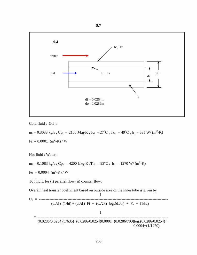
268
9.7
Cold fluid : Oil : mc = 0.3033 kg/s ; Cpc = 2100 J/kg-K ;Tci = 27oC ; Tco = 49oC ; hi = 635 W/ (m2-K) Fi = 0.0001 (m2-K) / W Hot fluid : Water : mh = 0.1083 kg/s ; Cph = 4200 J/kg-K ;Thi = 93oC ; ho = 1270 W/ (m2-K) Fo = 0.0004 (m2-K) / W To find L for (i) parallel flow (ii) counter flow: Overall heat transfer coefficient based on outside area of the inner tube is given by 1 Uo = ---------------------------------------------------------------------------------------------------- (do/di) (1/hi) + (do/di) Fi + (do/2k) loge(do/di) + Fo + (1/ho) 1 = ----------------------------------------------------------------------------------------------------- (0.0286/0.0254)(1/635)+(0.0286/0.0254)0.0001+(0.0286/700)loge(0.0286/0.0254)+ 0.0004+(1/1270)
9.4
di do oil
ho, Fo
k
hi , Fi
di = 0.0254m do= 0.0286m
water

269
9.8 = 325 W/(m2-K) Heat balance equation can be written as Q = mc x Cpc (Tco – Tci) = 0.3083 x 2100 ( 49 – 27 ) = 14243.5 W Also Q = mh Cph (Thi – Tho) Or Tho = Thi – Q/mh Cph = 93 – [14243.5/(0.1083x4200)] = 61.7oC (i) Parallel flow arrangement : ∆Ti = Thi – Tci = 93 – 27 = 66oC ∆To = Tho – Tco = 61.7 – 49 = 12.7oC hence MTD = ∆Tm = ∆Ti - ∆To / loge (66/12.7) = 32.34 o C Q = Uo π do L π ∆Tm Or L = Q / (Uo π do∆Tm) = 14243.5/(325 x π x 0.0286 x 32.34) = 15.1 m. (ii) Counter flow arrangement : ∆Tm = (93 – 49) – (61.7 – 27) / loge [(93 – 49) / (61.7 – 27)] = 39.2oC Hence L = 14243.5 / (325 x π x 0.0286 x 39.2) = 12.5 m

270
9.5 Solution: Shell side fluid : water : mc = 0.5 kg/s ; Cpc = 4200 J/kg-K ;Tci = 10oC ; Tube side fluid : Oil : mh = 0.3 kg/s ; Cph = 2000 J/kg-K ;Thi = 80oC ; Tho = 30oC U = 250 W/(m2-K) Heat balance equation is Q = mh Cph (Thi – Tho) = 0.3 x 2000 x (80 – 30) = 30000 W Also Q = mc x Cpc (Tco – Tci) Or Tco = Tci + Q/ mc Cpc = 10 + 30000/(0.5 x 4200) = 24.3oC (∆Tm)c.f = (80 – 24.3) – (30 – 10) / loge [(80 – 24.3) / (30 – 10)] = 34.35oC Single shell pass - two tube pass HE : T1 = 10 oC ; T2 = 24.3 oC ; t1 = 80 oC ; t2 = 30 oC R = T1 – T2 / t2 – t1 = 10 – 24.3 / 30 – 80 = 0.29 P = t2 – t1 / T1 – t1 = 30 – 80 / 10 – 80 = 0.714 From chart , F = 0.875 Hence (∆Tm) = F x (MTD)c.f = 0.875 x 34.85 = 30.5oC Q = U A (∆Tm) Or A = Q / U (∆Tm) = 30000/(250 x 30.5) = 3.93 m2

271
9.6 Solution: Cross flow HE : Cold water (Unmixed) : mc = 3 kg/s ; Cpc = 4200 J/kg-K ;Tci = 30oC ; Tco = 80oC ; Hot gases (Mixed) : Cph = 1005 J/kg-K ;Thi = 225oC ; Tho = 100oC U = 200 W/(m2/K) Q = mc x Cpc (Tco – Tci) = 3 x 4200 (80 – 30 ) = 630000 W Also P = t2 – t1 / T1 – t1 = 80 – 30 / 225 – 30 = 0.256 R = T1 – T2 / t2 – t1 = 225 – 100 / 80 – 30 = 2.5 From chart, F = 0.93 (∆Tm)c.f = (225 – 80) – (100 – 30) / loge [(225 – 80) / (100 – 30)] = 54.62oC (∆Tm) = 0.93 x 54.62 = 50.8oC Q = U A (∆Tm) or A = Q / A (∆Tm) = 630000 / (200 x 54.62) = 57.7 m2. 9.7 Solution: Water : mc = 2 kg/s; Cpc = 4200 J/kg-K ; Tci = 20oC ;Tco = 80oC ; Oil : Thi = 140oC ; Tho = 90oC U = 300 W / (m2 – K ) Q = mc x Cpc (Tco – Tci) = 2 x 4200 (80 – 20 )

272
= 504000 W Tube side fluid is water. Hence t1 = 20oC ; t2 = 80 oC Shell side fluid is oil. Hence T1 = 140 oC ; T2 = 90 oC P = t2 – t1 / T1 – t1 = 80 – 20 / 140 – 20 = 0.5 R = T1 – T2 / t2 – t1 = 140 – 90 / 80 – 20 = 0.83 From chart F = 0.97 (∆Tm)c.f = (140 – 80) – (90 – 20) / loge [(140 – 80) / (90 – 20)] = 64.87oC (∆Tm) = 0.97 x 64.87 = 60.9oC Q = U A (∆Tm) or A = Q / A (∆Tm) = 504000 / (300 x 62.9) = 26.7 m2. 9.8 Solution: Shell and Tube HE : Cold fluid : Water : mc = 8.33 kg/s ;Tci = 25oC ; Tco = 50oC ; Hot fluid : Steam condensing at atmospheric pressure. Hence Thi = Tho = Tsat at atmospheric pressure = 99.6o C (from steam tables) hfg = 2257 x 103 J / kg – K Tube side fluid is water. Hence hi = 3000 W / m2 – K Shell side fluid is oil. Hence ho = 8000 W / m2 – K Inside dia of tube = di = 0.025 m Outside dia of tube = do = 0.029 m

273
Length of the tube = L = 2 m Overall heat transfer coefficient based on outside surface area is given by 1 Uo = ---------------------------------------------------------------------------------------------------- (do/di) (1/hi) + (do/2k) loge(do/di) + (1/ho) As (do/2k) loge(do/di) = 0 1 = ----------------------------------------------------------------------------------------------------- (0.029 / 0.025) (1/3000) + ( 1 / 8000 ) = 1954 W/(m2-K) Since Thi = Tho , both parallel flow and counter flow arrangement will give the same value of (∆Tm). Hence (∆Tm) = (99.6 – 25) – (99.6 – 50 ) / loge [(99.6 – 25) / (99.6 – 50 ) ] = 61.2 oC Q = mc x Cpc (Tco – Tci) = 8.33 x 4200 (50 – 25 ) = 874650 W Q = Uo Ao (∆Tm) or Ao = Q / Uo (∆Tm) = 874650 / (1954 x 61.2) = 7.314 m2. Surface area of each tube = ao = π do L = π x 0.029 x 2 = 0.1822 m2 Hence number of tubes = n = Ao / ao = 7.314 / 0.1822 = 40.14 ≈ 41 B. Effectiveness - NTU method:
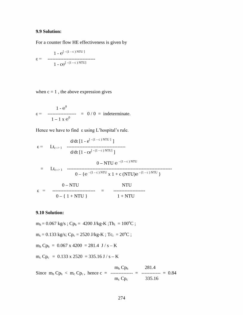
274
9.9 Solution: For a counter flow HE effectiveness is given by 1 - ℮[ - (1 – c ) NTU ] ε = ------------------------------ 1 - c℮[ - (1 – c ) NTU] when c = 1 , the above expression gives 1 - ℮0 ε = ------------------ = 0 / 0 = indeterminate. 1 – 1 x ℮0 Hence we have to find ε using L’hospital’s rule. d/dt [1 - e[ - (1 – c ) NTU ] ] ε = Ltc--> 1 ------------------------------------- d/dt [1 - ce[ - (1 – c ) NTU] ] 0 – NTU ℮ - (1 – c ) NTU = Ltc--> 1 ------------------------------------------------------------------ 0 – {℮ - (1 – c ) NTU x 1 + c (NTU)℮ - (1 – c ) NTU } 0 – NTU NTU ε = --------------------------- = -------------------- 0 – { 1 + NTU } 1 + NTU 9.10 Solution: mh = 0.067 kg/s ; Cph = 4200 J/kg-K ;Thi = 100oC ; mc = 0.133 kg/s; Cpc = 2520 J/kg-K ; Tci = 20oC ; mh Cph = 0.067 x 4200 = 281.4 J / s – K
mc Cpc = 0.133 x 2520 = 335.16 J / s – K mh Cph 281.4 Since mh Cph < mc Cpc , hence c = -------------- = ------------ = 0.84 mc Cpc 335.16
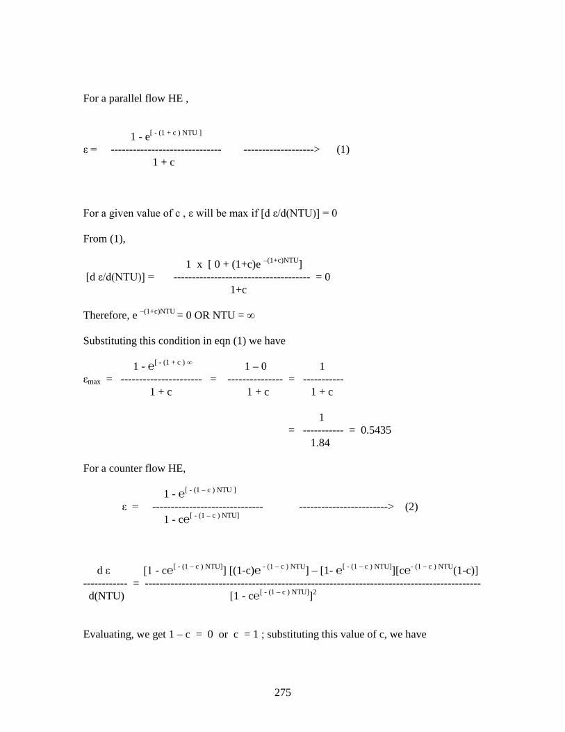
275
For a parallel flow HE , 1 - e[ - (1 + c ) NTU ] ε = ------------------------------ -------------------> (1) 1 + c For a given value of c , ε will be max if [d ε/d(NTU)] = 0 From (1), 1 x [ 0 + (1+c)e –(1+c)NTU] [d ε/d(NTU)] = ------------------------------------- = 0 1+c Therefore, e –(1+c)NTU = 0 OR NTU = ∞ Substituting this condition in eqn (1) we have 1 - ℮[ - (1 + c ) ∞ 1 – 0 1 εmax = ---------------------- = --------------- = ----------- 1 + c 1 + c 1 + c 1 = ----------- = 0.5435 1.84 For a counter flow HE, 1 - ℮[ - (1 – c ) NTU ] ε = ------------------------------ ------------------------> (2) 1 - c℮[ - (1 – c ) NTU] d ε [1 - c℮[ - (1 – c ) NTU]] [(1-c)℮ - (1 – c ) NTU] – [1- ℮[ - (1 – c ) NTU]][c℮- (1 – c ) NTU(1-c)] ------------ = ------------------------------------------------------------------------------------------- d(NTU) [1 - c℮[ - (1 – c ) NTU]]2
Evaluating, we get 1 – c = 0 or c = 1 ; substituting this value of c, we have

276
ε = 1 [ from (2) ] 9.11 Solution: Counter flow HE : mh = 3 kg/s ; Cph = 1050 J/kg-K ;Thi = 500oC ; mc = 0.75 kg/s; Cpc = 4200 J/kg-K ; Tco = 85oC ; U = 450 W / (m2- K ) mh Cph = 3 x 1050 = 3150 J / s – K mc Cpc = 0.75 x 4200 = 3150 J / s – K mh Cph = mc Cpc Hence Thi – Tho = Tco – Tci and c = 1 UA UA Also NTU = ------------------ or --------------------- mc Cpc mh Cph 450 x 1 = -------------- = 0.1428 3150 For a counter flow HE, 1 - ℮[ - (1 – c ) NTU ] ε = ------------------------------ 1 - c℮[ - (1 – c ) NTU]
NTU 0.1428 Since c = 1, ε = ---------------- = ------------------- = 0.1250 1 + NTU 1.1428 Thi – Tho Tco – Tci But ε = --------------- or ------------------ when c = 1 Thi – Tci Thi – Tci 85 - Tci Hence 0.1250 = ----------------- 500 - Tci
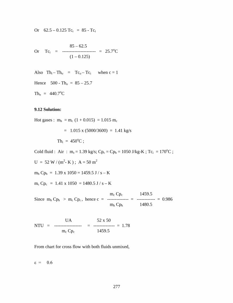
277
Or 62.5 – 0.125 Tci = 85 - Tci
85 – 62.5 Or Tci = ---------------------- = 25.7oC (1 – 0.125) Also Thi – Tho = Tco – Tci when c = 1 Hence 500 - Tho = 85 – 25.7 Tho = 440.7oC 9.12 Solution: Hot gases : mh = mc (1 + 0.015) = 1.015 mc = 1.015 x (5000/3600) = 1.41 kg/s Thi = 450oC ; Cold fluid : Air : mc = 1.39 kg/s; Cpc = Cph = 1050 J/kg-K ; Tci = 170oC ; U = 52 W / (m2- K ) ; A = 50 m2
mh Cph = 1.39 x 1050 = 1459.5 J / s – K mc Cpc = 1.41 x 1050 = 1480.5 J / s – K mc Cpc 1459.5 Since mh Cph > mc Cpc , hence c = -------------- = ------------ = 0.986 mh Cph 1480.5 UA 52 x 50 NTU = ------------------ = -------------- = 1.78 mc Cpc 1459.5 From chart for cross flow with both fluids unmixed, ε = 0.6

278
when mh Cph > mc Cpc , Tco – Tci ε = ------------------ Thi – Tci Or Tco = Tci + ε (Thi – Tci ) = 170 + 0.6 x [450 – 170 ] = 338 oC Also mc x Cpc (Tco – Tci) = mh x Cph (Thi – Tho) mc Cpc Hence Tho = Thi – ------------- x [ Tco – Tci ] mh Cph
= 450 - 0.986 [ 338 – 170 ] = 284.35 oC 9.13 Solution: Counter flow HE : case (i) Thi = 110o C ; Tho = 65o C ; Tci = 20o C ; Tco = 77oC ; L = 30 m ; U1 case (ii) Tci = 20o C ; Tco = 80oC ; Thi = 110o C ; U2 = U1 (assumed) For case (i) Q1 = mc x Cpc (Tco – Tci) = mc x Cpc ( 70 – 20 ) For case (ii) Q2 = mc x Cpc ( 80 – 20 ) Q1 mc x Cpc ( 70 – 20 ) 5 Hence, ------ = -------------------------------- = ------ Q2 mc x Cpc ( 80 – 20 ) 6 Also for case (i) mc x Cpc ( 70 – 20 ) = mh x Cph ( 110 – 65 ) Also for case (ii) mc x Cpc ( 80 – 20 ) = mh x Cph [ ( 110 – (Tho)2 ]

279
110 – 65 70 – 20 Hence --------------------- = -------------- 110 - (Tho)2 80 – 20 hence (Tho)2 = 110 – (6/5) [ 110 – 65 ] = 56
o C (110 – 70 ) – (65 – 20 ) Hence for case (i) (∆Tm)1 = ----------------------------------------- = 42.45oC loge [(110 – 70 ) / (65 – 20 )] (110 – 80 ) – (56 – 20 ) Hence for case (ii) (∆Tm)2 = ----------------------------------------- = 32.9 oC loge [(110 – 80 ) / (56 – 20 )] Q1 U1 π d L1 (∆Tm)1 5 hence , --------- = ---------------------- = ------- Q2 U2 π d L2 (∆Tm)2 6 L1 (∆Tm)1 5
Hence --------------------------- = ---------- L2 (∆Tm)2 6 Or L2 = (6/5) x [ (∆Tm)1 / (∆Tm)2 ] x L1
= (6/5) x (42.45/32.90) x 30 = 46.45 m 9.14 Solution: Solution by MTD method: Cross flow HE with oil mixed and water unmixed; Hot fluid : oil : mh = 0.278 kg/s ; Cph = 2087 J/kg-K ;Thi = 150oC ; Tho = 50oC Cold fluid : water : mc = 0.463 kg/s ; Cpc = 4200 J/kg-K ;Tci = 30oC; U = 550 W / (m2 – K ) Q = mc x Cpc (Tco – Tci) = 0.278 x 2087 [150 – 50 ] = 58019 W

280
Also Q = mh x Cph (Thi – Tho) Or Tco = Tci + (Q / mc Cpc) = 30 + [58019 / (0.463 x 4200 ) ] = 59.8 oC (∆Tm)c.f = (150 – 59.8) – (50 – 30) / loge [(150 – 59.8) / (50 – 30) ] = 46.6 oC R = (150 – 50 ) / (59.8 – 30 ) = 3.35 P = (59.8 – 30 ) / ( 150 – 30 ) = 0.25 From chart F = 0.80 (∆Tm) = 0.8 x 46.6 = 37.3 oC Q 58019 A = ------------- = --------------- = 2.83 m2 U (∆Tm) 550 x 37.3 Solution by ε – NTU method : mh Cph = 0.278 x 2087 = 580.2 J / s – K
mc Cpc = 0.463 x 4200 = 1944.6 J / s – K mh Cph 580.2 Since mh Cph < mc Cpc , hence c = -------------- = ------------ = 0.29 mc Cpc 1944.6 when mh Cph < mc Cpc , Thi – Tho 150 – 50 ε = ------------------ = ---------------- = 0.83 Thi – Tci 150 – 30 From chart, NTU = 2.8 = UA / (mCp)min = UA / mh Cph

281
Hence A = 2.8 x 530.2 / 550 = 2.95 m2 9.15) Cold: water: mc= 5000/3600 = 1.39 kg/s ; Tci= 30 oC ;Cpc= 4200 J/(kg-K) assumed Hot : oil : mh = 2000/3600 = 0.555 kg/s ;Cph = 2100 J/(kg-K) ;Thi= 90oC A= 3m2 ; U = 465 W/(m2-K) Case 1) Both the fluids flow in series. The arrangement for this case will be as shown with figure below:
As mcCpc = (5000/3600) x 4200 = 5833.3 J/(s-K) And mhCph= (2000/3600) x 2100 = 1166.7 J/(s-K) therefore mcCpc< mhCph
pipelines
Thi , mhcph
Tco
Tci , mhcph
Th*
Tho
Tc*
EXCHANGER 2
EXCHANGER 1
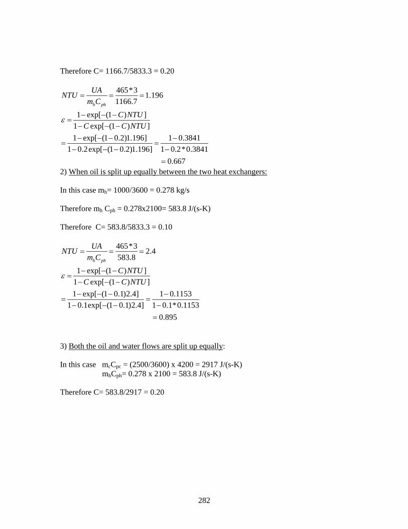
282
Therefore C= 1166.7/5833.3 = 0.20
465*3 1.1961166.7
1 exp[ (1 ) ]1 exp[ (1 ) ]1 exp[ (1 0.2)1.196] 1 0.3841
1 0.2exp[ (1 0.2)1.196] 1 0.2*0.38410.667
h ph
UANTUm C
C NTUC C NTU
ε
= = =
− − −=
− − −− − − −
= =− − − −
=
2) When oil is split up equally between the two heat exchangers: In this case mh= 1000/3600 = 0.278 kg/s Therefore mh Cph = 0.278x2100= 583.8 J/(s-K) Therefore C= 583.8/5833.3 = 0.10
465*3 2.4583.8
1 exp[ (1 ) ]1 exp[ (1 ) ]1 exp[ (1 0.1)2.4] 1 0.1153
1 0.1exp[ (1 0.1)2.4] 1 0.1*0.11530.895
h ph
UANTUm C
C NTUC C NTU
ε
= = =
− − −=
− − −− − − −
= =− − − −
=
3) Both the oil and water flows are split up equally: In this case mcCpc = (2500/3600) x 4200 = 2917 J/(s-K) mhCph= 0.278 x 2100 = 583.8 J/(s-K) Therefore C= 583.8/2917 = 0.20

283
465*3 2.4583.8
1 exp[ (1 ) ]1 exp[ (1 ) ]1 exp[ (1 0.2)2.4] 1 0.1467
1 0.2exp[ (1 0.2)2.4] 1 0.02930.879
h ph
UANTUm C
C NTUC C NTU
ε
= = =
− − −=
− − −− − − −
= =− − − −
=
Since ε is the highest in case (2), this arrangement is the best for ” maximizing heat transfer” point of view. 9.16 Solution:
U1 = U2 = U = 850 W / (m2 – K ) Case (i) single counter flow HE : Q = mc x Cpc (Tco – Tci) = 1.25 x 4200 [80 – 35 ] = 236250 W Q = mh x Cph (Thi – Tho)
9.16
EXCHANGER 1
EXCHANGER 2
Oil (mh), Cph= 2000 J/kg-k Thi= 150oC
mh/2 mh/2 Tci = 35oC mc =1.25 kg/s
Tc*
Thi
Tho=85oC
Th1* Th2*
Tco=80oC
284
Q 236250 Hence mh = ------------------------ = ---------------------------- = 1.817 kg/s Cp [Thi – Tho] 2000 x [150 – 85 ] mh Cph = 1.817 x 2000 = 3634.6 J / s – K
mc Cpc = 1.25 x 4200 = 5250 J / s – K mh Cph 3634.6 Since mh Cph < mc Cpc , hence c = -------------- = ------------ = 0.7 mc Cpc 5250 Thi – Tho 150 – 85 ε = ------------------ = ------------------- = 0.565 Thi – Tci 150 – 35 From chart, NTU = 1.0 = UA / (mCp)min = UA / mh Cph Hence A = 1 x 3634.6 / 850 = 4.276 m2
Case (ii) When two smaller heat exchangers are used: For this case mh = 1.317 / 2 = 0.9085 kg/s mh Cph = 0.9085 x 2000 = 1817 J / s – K
mc Cpc = 1.25 x 4200 = 5250 J / s – K Hence c = 1817 / 5250 = 0.35 To find ‘ε’ , we should know the exit temperatures of hot and cold fluids for at least one HE. Since UA and (mCp)min is the same for both the exchangers NTU should be same for both the exchangers. Thi – Th1* Thi – Th2* Thus ε1 = ------------------ = ε2 = ---------------- Thi – Tci Thi – Tc*
Therefore *
21 2*
150 150 ..............................(1)150 35 150
hi h
c
T TT
ε ε− −= = =
− −

285
Since the oil flow is the same in each exchanger and the average exit oil temperature must be 85oC …..it follows that
* *
1 2 85 ........................................(2)2
oh hT T C+=
Energy balance on the second heat exchanger gives
* *25250(80 ) 1817(150 )..................................(3)c hT T− = −
Equations 1,2 ,3 may be solved for the three unknowns Th1
* , Th2* , Tc
* . The solutions are as follows: Eqn 1can be rearranged after cross multiplying as:
* * * * *1 2 1150 115 150 5250........................(4)h h c h cT T T T T− + − =
Eqn 2……………… * *1 2 170........................................(5)h hT T+ =
Eqn 3……………….. * *2 2.9 82.....................................(6)h cT T− = −
From eqn 6………………
** *2
282 0.345 28.3
2.9h
c hTT T+
= = +
From eqn 5………………. * *1 2170h hT T= −
Substituting these expressions in Eqn 4 we have: * * * * *
2 2 2 2 2150(170 ) 115 150(0.345 28.3) (170 )(0.345 28.3) 5250h h h h hT T T T T− − + + − − + = Or *2 *
2 2706 57055 0h hT T− + =
Therefore 2
*2
706 706 4*57055 93 6132hT or± −
= =
Th2* cannot be 613 oC.
Therefore………. *
2 93ohT C=
Therefore……….. *
1 170 93 77ohT C= − =
And…………….. * 0.345*93 28.3 60.4o
cT C= + =
Therefore……………. 1 2150 77 0.635150 33
ε ε −= = =
−
Therefore from chart, 1.16NTU =

286
Therefore…………….. 21 2
1817*1.16 2.48850
A m A= = =
Therefore total area required to meet the heat load = 2.482*2= 4.92m2 This is more than the 4.276 m2 required in the one larger heat exchanger. In addition the cost per unit area is greater so that the most economical choice from the heat transfer point of view would be the single large heat exchanger.
287
CHAPTER: 10
RADIATION HEAT TRANSFER
10.1. INTRODUCTORY CONCEPTS AND DEFINITIONS 10.1.1 THERMAL RADIATION When a body is placed in an enclosure whose walls are at temperatures below that of the body, the temperature of the body will decrease even if the enclosure is evacuated. This process by which heat is transferred from a body by virtue of its temperature, without the aid of any intervening medium is called “THERMAL RADIATION”. The actual mechanism of radiation is not yet completely understood. There are at present two theories by means of which radiation propagation is explained. According to Maxwell’s electromagnetic theory, Radiation is treated as electromagnetic waves, while Max Planck’s theory treats radiation as “Photons” or “Quanta of energy”. Neither theory completely describes all observed phenomena. It is however known that radiation travels with the speed of light, c (c = 3x10⁸ m/s) in a vacuum. This speed is equal to the product of the frequency of the radiation and the wavelength of this radiation, OR c = λν ………………………………….(10.1) Where λ = wavelength of radiation (m) and ν = frequency (1/s). Usually, it is more convenient to specify wavelength in micrometer, which is equal to 10-6 m. From the viewpoint of electromagnetic wave theory, the waves travel at the speed of light, while from the quantum theory point of view, energy is transported by photons which travel at the speed of light. Although all the photons have the same velocity, there is always a distribution of energy among them. The energy associated with a photon, ep = hν where h is the Planck’s constant equal to 6.6256 x 10⁻³⁴ Js. The entire energy spectrum can also be described in terms of the wavelength of radiation. Radiation phenomena are usually classified by their characteristic wavelength, λ. At temperatures encountered in most engineering applications, the bulk of the thermal energy emitted by a body lies in the wavelengths between λ= 0.1 and 100 μm. For this reason, the portion of the wavelength spectrum between λ= 0.1 and 100 μm is generally referred to as “THERMAL RADIATION”. The wavelength spectrum in the range λ= 0.4 and 0.7 μm is visible to the naked eye, and this is called ‘light rays’. The wavelength spectrum of radiation is illustrated in Fig 10.1

288
Fig. 10.1 Typical Spectrum of electromagnetic radiation
In the study of radiation transfer, a distinction should be made between bodies
which are “semi-transparent” to radiation and those which are “opaque”. If the material is semitransparent to radiation, such as glass, salt crystals, and gases at elevated temperatures, then the radiation leaving the body from its outer surfaces results from emissions at all depths within the material. The emission of radiation for such cases is a “BULK” or a “VOLUMETRIC PHENOMENON”. If the material is opaque to thermal radiation, such as metals, wood, rock etc. then the radiation emitted by the interior regions of the body cannot reach the surface. In such cases, the radiation emitted by the body originates from the material at the immediate vicinity of the surface (i.e. within about 1μm) and the emission is regarded as a “SURFACE PHENOMENON”. It should also be noted that a material may behave as a semi transparent medium for certain temperature ranges, and as opaque for other temperatures. Glass is a typical example for such behaviour. It is semi transparent to thermal radiation at elevated temperatures and opaque at intermediate and low temperatures. 10.1.2 DEFINITIONS OF TERMS USED IN THERMAL RADIATION
• Monochromatic Emissive Power (Eλ): The monochromatic emissive power of a surface at any temperature T and wavelength λ is defined as the quantity which when multiplied by dλ gives the radiant flux in the wavelength range - λ to λ+dλ.
• Emissive Power (E): The emissive power of a surface is the energy emitted by a
surface at a given temperature per unit time per unit area for the entire wavelength range, from λ = 0 to λ = ∞.
10.2
Thermal Radiation
( 0.1 μm to 100 μm )
Light Rays (0.1 μm to 0.3 μm)
Infrared Radiation (0.7 to 103 μm)
Ultra violet radiation (10 −2 to 0.4 μm)
λ , μm
10−5 10
−4 10−3
10−2 10
−1 100
10 102
103 10
4 10
5

289
10.3
∞ E = ∫Eλdλ ……………………………………………(10.2)
0
• Absorptivity, Reflectivity and Transmissibility of a body:
Fig.10.2: Effects of radiation incident on a surface
When a radiant energy strikes a material surface, part of the radiation is reflected,
part is absorbed, and part is transmitted, as shown in Fig. 10.2. Reflectivity (ρ) is defined as the fraction of energy which is reflected, Absorptivity (α) as the fraction absorbed, and Transmissivity (τ) as the fraction transmitted. Thus, ρ + α + τ = 1.
Most solid bodies do not transmit thermal radiation, so that for many applied problems, the transmissivity may be taken as zero. Then ρ + α = 1 ……………………………………(10.3)
Incident Radiation Energy reflected
Energy Absorbed
Energy transmitted

290
10.4
• Specular Radiation and Diffuse Radiation:
Fig.10.3: Specular and Diffuse Radiation
When radiation strikes a surface, two types of reflection phenomena may be
observed. If the angle of incidence is equal to the angle of reflection, the radiation is called Specular. On the other hand, when an incident beam is distributed uniformly in all directions after reflection, the radiation is called Diffuse Radiation. The two types of radiation are depicted in Fig. 10.3. Ordinarily, no real surface is either specular or diffuse. An ordinary mirror is specular for visible light, but would not necessarily be specular over the entire wavelength range. A rough surface exhibits diffuse behaviour better than a highly polished surface. Similarly, a highly polished surface is more specular than a rough surface. • Black Body:
A body which absorbs all incident radiation falling on it is called a blackbody. For
a blackbody, α = 1, ρ = τ = 0. For a given temperature and wavelength, no other body at the same temperature and wavelength, can emit more radiation than a blackbody. Blackbody radiation at any temperature T is the maximum possible emission at that temperature. A blackbody or ideal radiator is a theoretical concept which sets an upper limit to the emission f radiation. It is a standard with which the radiation characteristics of other media are compared. • Emissivity of a Surface (ε):
The emissivity of a surface is the ratio of the emissive power of the surface to the emissive power of a black surface at the same temperature. It is denoted by the symbol ε.
Ф2 = Φ1
(a) Specular Radiation (b) Diffuse Radiation
Source
Φ1 Φ2
Source

291
10.5
i.e. ε = [E/Eb]T. • Monochromatic Emissivity of a Surface (ελ):
The monochromatic emissivity of a surface is the ratio of the monochromatic
emissive power of the surface to the monochromatic emissive power of a black surface at the same temperature and same wavelength.
ελ = [Eλ / Ebλ ] λ,T.
• Gray Body: A gray body is a body having the same value of monochromatic emissivity
at all wavelengths. i.e. ε = ελ, for a gray body. • Radiosity of a Surface (J):
This is defined as the total energy leaving a surface per unit time per unit area of
the surface. This definition includes the energy reflected by the surface due to some radiation falling on it.
• Irradiation of a surface(G):
This is defined as the radiant energy falling on a surface per unit time, per unit
area of the surface. Therefore if E is the emissive power, J is the radiosity, ε is the irradiation and ρ
the reflectivity of a surface, then, J = E + ρG
For an opaque surface, ρ + α = 1 or ρ = (1 – α) J = E + (1-α)G …………………………………………. (10.4)
10.2 LAWS OF RADIATION 10.2.1 STEFAN – BOLTZMANN LAW: This law states that the emissive power of a blackbody is directly proportional to the fourth power of the absolute temperature of the body.
i.e., Eb α T4
Or Eb = σT4 ---------------------------------- (10.5) where σ is called the Stefan – Boltzmann constant.
In SI units σ = 5.669x10⁻⁸ W/(m2-K4).
292
10.6 10.2.2 PLANCK’S LAW: This law states that the monochromatic power of a blackbody is given by C1
Ebλ = ------------------------------ ………………………..(10.6) λ5 [ e (C2
/ λT) – 1] where C1 and C2 are constants whose values are found from experimental data;
C1 = 3.7415 x 10⁻¹⁶ Wm2 and C2 = 1.4388 x 10⁻² m-K. λ is the wavelength and T is the absolute temperature in K.
10.2.3 WEIN’S DISPLACEMENT LAW: It can be seen from Eq. 10.6 that at a given temperature, Ebλ depends only on λ. Therefore the value of λ which gives maximum value of Ebλ can be obtained by differentiating Eq(10.6) w.r.t λ and equating it to zero. Let C2/λT = y . Then Eq. (10.6) reduces to C1 Ebλ = -----------------------------
[C2 / (yT)] 5 [ e y – 1] Then dEbλ C1 d / dy {[C2 / (yT)] 5 [ e y – 1]} ------ = ------------------------------------------ dy {[C2 / (yT)] 5 [ e y – 1]} 2 or d / dy {[C2 / (yT)] 5 (e y – 1)} = 0
Or ey(5 – y) = 5 By trial and error, y = 4.965 Therefore, if λm denotes the value of λ which gives maximum Ebλ, then
C2/λmT = 4.965 Or λmT = C2/4.965 = 1.4388x10⁻² /4.965
λmT = 0.002898 m-K ………………………………. (10.7)

293
10.7 Equation (10.7) is called the Wein’s displacement law. From this equation it can be seen that the wavelength at which the monochromatic emissive power is a maximum decreases with increasing temperature. This is also illustrated in Fig 10.4(a). Fig 10.4(b) gives a comparison of monochromatic emissive powers for different surfaces at a particular temperature for different wavelengths.
Fig. 10.4 (a) Black body emissive power as a function of wave length
and Temperature
Fig. 10.4 (b) Comparison of emissive powers of different types o
surfaces as a function of wavelength at a given temperature
Ebλ
0 1 2 3 4 5 6
300 250 200 150 100
1990 K
1360 K
Wavelength
Monochromatic emissive power
Wavelength
Black body (ελ = ε = 1)
Gray body (ελ = ε < 1)
Real Surface

294
10.8 10.2.4 KIRCHOFF’S LAW: This law states that the emissivity of a surface is equal to its absorptivity when the surface is in thermal equilibrium with the surroundings. Proof: Consider a perfect black enclosure i.e. the one which absorbs all the incident radiation falling on it (see Fig 10.5). Now let the radiant flux from this enclosure per unit area arriving at some area be qi W/m2.
Fig. 10.5 : Model used for deriving Kirchoff law Now suppose that a body is placed inside the enclosure and allowed to come to thermal equilibrium with it. At equilibrium, the energy absorbed by the body must be equal to the energy emitted; otherwise there would be an energy flow into or out of the body, which would raise or lower its temperature. At thermal equilibrium we may write
EA = qi A α ………………………………….(10.8) If we now replace the body in the enclosure with a black body of the same size and shape and allow it to come to thermal equilibrium with the enclosure, EbA = qi A .......………………………………(10.9) Since α = 1 for a blackbody. If Eq. 10.8 is divided by Eq. 10.9 we get E/Eb = α But by definition E/Eb = ε, the emissivity of the body, so that ε = α…………(10.10)
Sample
Black Enclosure
qi.A.α
EA

295
10.9
Equation 10.10 is called Kirchoff’s law and is valid only when the body is in thermal equilibrium with the surroundings. However, while analyzing radiation problems in practice we assume that Kirchoff’s law holds good even if the body is not in thermal equilibrium with the surroundings, as the error involved is not very significant. 10.3 ILLUSTRATIVE EXAMPLES ON BASIC CONCEPTS Example 10.1: The emission of radiation from a surface can be approximated as blackbody radiation at 1000K.
(a) What fraction of the total energy emitted is below λ = 5μm (b) What is the wavelength below which the emission is 10.5% of the total emission at
1000K. (c) What is the wavelength at which the maximum spectral emission occurs at 1000K.
Solution: The radiation flux emitted by the blackbody over the wavelength interval 0 – λ is given by λ [Eb]0 – λ = ∫Ebλdλ
0 The integration required in the above equation has been done numerically and the results are presented in the form of a table. The table gives the value of D 0-λ where λ ∫Ebλdλ 1 λ D0-λ = ---0-∞----------- = ------- ∫ Ebλ dλ ∫Ebλdλ σ T4 0 0
(a) From Table of Radiation properties, for λT = 5 x 1000 = 5000, D0-λ = 0.6337. This means that 63.37 % of the total emission occurs below λ = 5 μm.
(b) From the same table, for D0-λ = 0.105, λT = 2222. Hence λ = 2222/1000 = 2.222 μm. (c) From Wein’s displacement law, λmT = 0.002898. Hence for T = 1000 K, λm =0.002898 / 1000 = 2.898 x 10 −6 m = 2.898 μm. Example 10.2: The monochromatic emissivity of a surface varies with the wavelength in the following manner: ελ = 0 for λ < 0.3μm = 0.9 for 0.3μm < λ < 1μm = 0 for λ > 1μm Calculate the heat flux emitted by the surface if it is at a temperature of 1500 K

296
10.10
Solution: Eλ = ε λ Ebλ
∞ 0.3 μm 1 μm ∞ Therefore E = ∫ ε λ Ebλ = ∫ 0.0 Ebλ dλ + ∫ 0.9 Ebλ dλ + ∫ 0.0 Ebλ dλ
0 0
0.3 μm 1 μm
1 μm 1 μm 0.3 μm = 0.9 ∫Ebλ dλ = 0.9 [ ∫ Ebλ dλ − ∫ Ebλ dλ ]
0.3 μm
0 0 = 0.9 σ T 4 [ D0-1 – D0 – 0.3]
For λ = 1μm, λT = 1500 μm-K, therefore D0-1 = ½ (0.01972 + 0.00779) = 0.93755 For λ = 0.3μm, λT = 450 μm-K, therefore D0-3 = 0 Thus E = 0.9x5.67x10-8x15004 [0.013755 – 0] = 3553 W/m2 Example 10.3: Calculate the heat flux emitted due to thermal radiation from a black surface at 60000 C. At what wavelength is the monochromatic emissive power maximum and what is the maximum value? Solution:Temp of the black surface = 6273K Heat Flux emitted = Eb = σT4 = 5.67x10-8x62734 = 87798 KW/m2 Wavelength corresponding to max monochromatic emissive power is given by λmT = 0.002898 m-K λm = 0.002898/6273 = 4.62x10⁻⁷ m
The maximum monochromatic emissive power is given by 2 π C1 (Ebλ)max = ------------------------------------ λmax [ exp {C2 / (λmaxT)} – 1] 2 x π x 0.596 x 10 − 16
= --------------------------------------------------------------- (4.62 x 10 − 7) 5 x [ exp{ 0.014387 / 0.002898} – 1] = 1.251 x 10 14 W / m2
297
10.11 Example 10.4: The spectral hemispherical emissivity (monochromatic emissivity) of fire brick at 750K as a function of wavelength is as follows: ε1 = 0.1 for 0 < λ < 2μm ε2 = 0.6 for 2μm < λ < 14μm ε3 = 0.8 for14 < λ < ∞ Calculate the hemispherical emissivity, ε for all wavelengths. Solution: ∞ E ∫ελ Ebλ dλ 1 λ1 λ2 λ3 ε = ------ = -0------------- = ------ [ ε1 ∫ Ebλ dλ + ε2 ∫ Ebλ dλ + ε3 ∫ Ebλ dλ ] Eb σ T 4 σ T 4 0 λ1 λ2 Where λ1 = 2μm, λ2 = 14μm, λ3 = ∞ Thus = ε1D0-λ1 + ε2[D0-λ2 – D0-λ1] + ε3[D0-∞ – D0-λ2] Now, λ1T = 2x750 = 1500; D0-λ1 = 0.013 λ2T = 14x750 = 10500; D0-λ2 = 0.924 λ3T = ∞; D0-λ3 = 1 Hence ε = 0.1 x 0.013 + 0.6 x [ 0.924 – 0.013] + 0.8 x [1 – 0.924] = 0.609 Example 10.5: the filament of a light bulb is assumed to emit radiation as a black body at 2400K. if the bulb glass has a transmissivity of 0.90 for radiation in the visible range, calculate the percentage of the total energy emitted by the filament that reaches the ambient as visible light. Solution: The wavelength range corresponding to the visible range is taken as λ1 = 0.38μm to λ2 = 0.76μm. Therefore the fraction F of the total energy emitted in this range is given by λ2 ∫ Ebλ dλ λ2 λ1 F = τ [λ1--------- ] = τ [ ∫Ebλ dλ − ∫Ebλ dλ ] / Eb Eb (T)
0 0
= τ [D0-λ2 – D0-λ1]. Now λ1T = 0.38 x 2400 = 912. Hence D0-λ11 = 0.0002 and λ2T = 0.76 x 2400 = 1824. Hence D0-λ2 = 0.0436 Therefore F = 0.9 x [0.0436 – 0.0002] =0.039 .
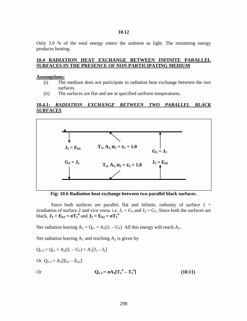
298
10.12 Only 3.9 % of the total energy enters the ambient as light. The remaining energy produces heating. 10.4 RADIATION HEAT EXCHANGE BETWEEN INFINITE PARALLEL SURFACES IN THE PRESENCE OF NON PARTICIPATING MEDIUM Assumptions:
(i) The medium does not participate in radiation heat exchange between the two surfaces.
(ii) The surfaces are flat and are at specified uniform temperatures. 10.4.1: RADIATION EXCHANGE BETWEEN TWO PARALLEL BLACK SURFACES
Fig: 10.6 Radiation heat exchange between two parallel black surfaces.
Since both surfaces are parallel, flat and infinite, radiosity of surface 1 = irradiation of surface 2 and vice versa. i.e. J1 = G2 and J2 = G1. Since both the surfaces are black, J1 = Eb1 = σT1
4 and J2 = Eb2 = σT24
Net radiation leaving A1 = Qr1 = A1(J1 – G1) All this energy will reach A2. Net radiation leaving A1 and reaching A2 is given by Q1-2 = Qr1 = A1(J1 – G1) = A1[J1 – J2]
Or Q1-2 = A1[Eb1 – Eb2]
Or Q1-2 = σA1[T14 – T2
4] (10.11)
J1 = Eb1
G2 = J1
G1 = J2
J2 = Eb2
T1, A1, α1 = ε1 = 1.0
T2, A2, α2 = ε2 = 1.0

299
10.13
10.4.2 RADIATION HEAT EXCHANGE BETWEEN TWO PARALLEL INFINITE GRAYSURFACES:
Fig: 10.7 Radiation Heat Exchange Between 2 Parallel Infinite Gray Surfaces.
Since the net radiation leaving A1 will reach A2, Q1-2 = Qr1 = A1[J1 – G1] (10.12a) J1 = E1 + (1-α1)G1 (10.12b) J2 = E2 + (1-α2)G2 (10.12c) J1 = G2 (10.12d) J2 = G1 (10.12e) Equation (10.12b) can be written as J1 – (1 – α1)G1 = E1 ……………………………..(4.12f) Equation (4.12c) with the help of Eqns. (10.12d) and Eqns. (10.12e) can be rewritten as
– (1 – α2)J1 + G1 = E2 (10.12g)
J1
G2 = J1
G1 = J2
J2
T1, α1= ε1, A1
T2, α2 = ε2, A2
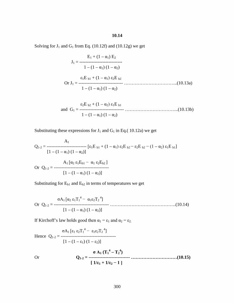
300
10.14
Solving for J1 and G1 from Eq. (10.12f) and (10.12g) we get E1 + (1 – α1) E2 J1 = ---------------------------- 1 – (1 – α1) (1 – α2) ε1E b1 + (1 – α1) ε2E b2 Or J1 = ----------------------------- ……………………………..(10.13a) 1 – (1 – α1) (1 – α2) ε2E b2 + (1 – α2) ε1E b1 and G1 = ----------------------------- ……………………………..(10.13b) 1 – (1 – α1) (1 – α2) Substituting these expressions for J1 and G1 in Eq.( 10.12a) we get A1 Q1-2 = -------------------------- [ε1E b1 + (1 – α1) ε2E b2 − ε2E b2 − (1 – α2) ε1E b1] [1 – (1 – α1) (1 – α2)] A1 [α2 ε1Eb1 − α1 ε2Eb2 ] Or Q1-2 = ------------------------------------ [1 – (1 – α1) (1 – α2)] Substituting for Eb1 and Eb2 in terms of temperatures we get σA1 [α2 ε1T1
4 − α1ε2T2 4]
Or Q1-2 = ------------------------------------ …………………………………….(10.14) [1 – (1 – α1) (1 – α2)] If Kirchoff’s law holds good then α1 = ε1 and α2 = ε2. σA1 [ε1 ε2T1
4 − ε1ε2T2 4]
Hence Q1-2 = ------------------------------------ [1 – (1 – ε1) (1 – ε2)] σ A1 (T1
4 – T24)
Or Q1-2 = --------------------------- …………………………(10.15) [ 1/ε1 + 1/ε2 − 1 ]

301
10.15 10.4.3 PLANE RADIATION SHIELDS: It is possible to reduce the net radiation heat exchange between two infinite parallel gray surfaces by introducing a third surface in between them. If the third surface, known as the radiation shield is assumed to be very thin, then both sides of this surface can be assumed to be at the same temperature.
Fig.10.8 shows a scheme for radiation heat exchange between two parallel infinite
gray surfaces at two different temperatures T1 and T2 in presence of a radiation shield at a uniform temperature, T3.
Now Q1-3 σ (T1
4 – T34)
------ = --------------------------- ………………………..(10.16a) A1 [ 1/ε1 + 1/ε13 – 1] Q3-2 σ (T3
4 – T24)
And ------ = --------------------------- ………………………..(10.16b) A1 [ 1/ε32 + 1/ε2 – 1]
Fig: 10.8 Radiation Heat Exchange Between Two Parallel Infinite Gray surfaces in presence of a radiation shield
For steady state conditions, these two must be equal..Therefore we have (T1
4 – T34) (T3
4 – T24)
--------------------------- = ---------------------------- [ 1/ε1 + 1/ε13 – 1] [ 1/ε32 + 1/ε2 – 1] Let X = [ 1/ε1 + 1/ε13 – 1] and Y = [ 1/ε32 + 1/ε2 – 1]
T1, α1= ε1, A1
T2, α2 = ε2, A2
T3, ε13, A3 = A1
T3, ε23, A3 = A1

302
10.16 Then, (T1
4 – T34) (T3
4 – T24)
--------------- = ------------------ X Y Solving for T3 we get T1
4 + (X/Y)T24
T3 = [ ----------------------------- ] 1 / 4 …………………(10.16c) (1 + X /Y)
Substituting this value of T3 in Eq. (10.16a) we get
Q1-3 / A1 = Q3-2 / A1 = (Q1-2 / A)1 Rad.Shield = σ { T24 – [{T1
4 +(X/Y)T24}/(1 + X/Y)] } / X
…………………….(10.17a) Special case: When ε1 = ε2 = ε13 = ε32 = ε, then X = Y = (2/ε) − 1 Hence, T3 = [(T1
4+ T24) / 2 ] ¼ ………………………..(10.18a)
σ{ T1
4 − [(T14 + T2
4) / 2 ] and [Q1-2 / A ]1 rad shield = ------------------------------------- [2/ε − 1] σ [T1
4 − T24]
= ------------------------ ………………………………(10.18b) 2 [2/ε − 1]
It can be seen from the above equation that when the emissivities of all surfaces are equal, the net radiation heat exchange between the surfaces in the presence of single radiation shield is 50% of the radiation heat exchange between the same two surfaces without the presence of a radiation shield. This statement can be generalised for N radiation shields as follows: 1 [Q1-2 / A]N shields = --------- [Q1-2 / A] without shield ……………(10.18c) (N + 1)

303
10.17 4.5: ILLUSTRATIVE EXAMPLES ON PLANE RADIATION SHIELDS Example 10.6: Two parallel infinite grey surfaces of emissivities 0.5 are at temperatures of 400K and 300K. Determine the net radiation heat flux between the two surfaces. Also determine the reduction in radiation flux when a plane radiation shield having emissivity of 0.5 on both its surfaces is placed between the two grey surfaces. Also determine the steady state temperature of the shield. Solution: The radiation flux between two gray surfaces is given by σ (T1
4 – T2 4) q = Q1-2 / A = -------------------------- .
[ 1 / ε1 + 1 / ε2 – 1]
5.67 x 10 − 8 x (400 4 – 300 4) Since ε1 = ε2 = ε = 0.5, we have q = ------------------------------------- (2 / 0.5 – 1) Or q = 330.75 W / m2. When a radiation shield of same emissivity is placed between two grey surfaces, the temperature of the shield T3 is given by T3 = [(T1
4 + T24) / 2 ] ¼
Hence T3 = [(400 4 + 300 4) / 2] ¼ Or, T3 = 360.3 K Also, since the emissivities of the plates and shield are equal we have (q)1 shield = q / 2 = 330.75 / 2 = 163.375 W /m2
Example 10.7: Two parallel plates are at temperatures T1 and T2 and have emissivities ε1 = 0.8 and ε2 = 0.5. A radiation shield having the same emissivity ε3 on both sides is placed between the plates. Calculate the emissivity ε3 of the shield in order to reduce the radiation heat loss from the system to one tenth of that without shield. Solution: Radiation flux between the two plates without the presence of a radiation shield is given by

304
10.18 σ [ T1
4 − T24 ] σ [ T1
4 − T24 ]
q1-2 = ------------------------- = --------------------------- [ 1 / ε1 + 1 / ε2 − 1 ] [ 1 / 0.8 + 1 / 0.5 − 1] σ [ T1
4 − T24 ]
or q1-2 = -------------------- …………………………(1) 2.25 When a shield is placed between the plates, the radiation flux is given by
( )
( )
( ) ( )
4 44 1 2
1
1
1 3 3 3
3 2 3 3
4 4 41 1 2
1
4 41 2
1
( / )1 /
1 1 1 1 11 1 0.250.8
1 1 1 1 11 1 10.5
(1 / ) ( / )(1 / )
radshield
radshield
radshield
T x y TTx y
qx
x
y
x y T T x y Tq
x x y
T Tq
x y
σ
ε ε ε ε
ε ε ε ε
σ
σ
+− + =
= + − = + − = +
= + − = + − = +
+ − − ∴ =+
−=
+
But (q)1radshield = 0.1 x q1-2
( ) ( )4 4 4 41 2 1 2
3 3
33
1 1 122.5 0.25 1 22.510 2.25
2 221.25 0.09421.25
T T T Tx y
x yσ σ
ε ε
εε
− −∴ = ⇒ + = ⇒ + + + =
+
⇒ = ⇒ = =
Example 10.8: Two large parallel plates are at 800K and 600K have emissivities of 0.5 and 0.8 respectively. A radiation shield having emissivity of 0.1 on the surface facing 800K plate and 0.05 on the surface facing 600K plate is placed between the plates. Calculate the heat transfer rate per m2 with and without the shield. Also calculate the temperature of the shield. Solution: The radiation flux without the radiation shield is given by σ (T1
4 – T24) 5.67 x 10 − 8 x (800 4 – 600 4)
q = ------------------------ = -------------------------------------- = 7056 W / m 2
[ 1 / ε1 + 1 / ε2 – 1] [ 1 / 0.5 + 1 / 0.8 – 1]

305
10.19 When a radiation field is placed between thick plates the radiation flux is given by σ (T1
4 – T34)
(q)1 Rad. shield = ------------------------- where x = [ 1 / ε1 + 1 / ε13 – 1] x T1
4 + (x/y) T24
and T3 = [ ------------------ ] ¼ where y = [ 1 / ε32 + 1 / ε2 – 1] 1 + (x/y) Now x = [ 1 / 0.5 + 1 / 0.1 – 1] = 11 and y = [1 / 0.05 + 1 / 0.8 – 1] = 20.25 800 4 + (11/20.25) x 600 4 Therefore T3 = [------------------------------- ] 1/4
1 + (11 / 20.25) = 746.8 K 5.67 x 10 − 8 x (800 4 – 746.8 4) Hence (q)1 Rad. shield = ---------------------------------------- = 508 W / m 2
11 Example 10.9: Find an expression for the net radiant flux between two infinite parallel diffuse grey surfaces at temperatures T1 and T2 degrees Kelvin when an infinite opaque plate of thickness b and thermal conductivity K is placed between them. Assume that all surfaces have the same emissivity. Solution: The schematic for the problem is shown in Fig. E10.9. For steady state heat transfer we have q = Q1-2 / A = Q1-3 / A = Q3-4 / A = Q4-2 / A σ (T1
4 – T34)
Now Q1-3 / A = ------------------------ …………………………………………….(1) (2/ε – 1) Q3-4 / A = k (T3 – T4) / b ……………………………………………………(2)
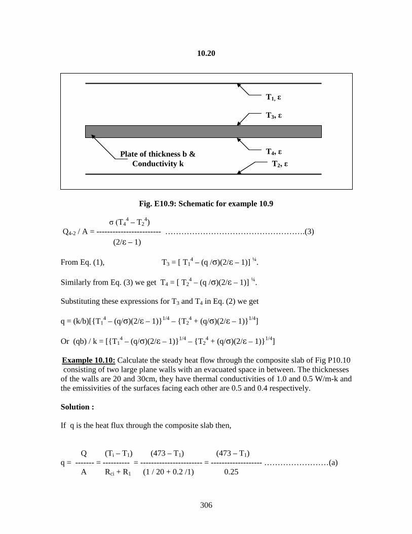
306
10.20
Fig. E10.9: Schematic for example 10.9
σ (T4
4 – T24)
Q4-2 / A = ------------------------ …………………………………………….(3) (2/ε – 1) From Eq. (1), T3 = [ T1
4 – (q /σ)(2/ε – 1)] ¼. Similarly from Eq. (3) we get T4 = [ T2
4 – (q /σ)(2/ε – 1)] ¼. Substituting these expressions for T3 and T4 in Eq. (2) we get q = (k/b)[{T1
4 – (q/σ)(2/ε – 1)}1/4 – {T24 + (q/σ)(2/ε – 1)}1/4]
Or (qb) / k = [{T1
4 – (q/σ)(2/ε – 1)}1/4 – {T24 + (q/σ)(2/ε – 1)}1/4]
Example 10.10: Calculate the steady heat flow through the composite slab of Fig P10.10 consisting of two large plane walls with an evacuated space in between. The thicknesses
of the walls are 20 and 30cm, they have thermal conductivities of 1.0 and 0.5 W/m-k and the emissivities of the surfaces facing each other are 0.5 and 0.4 respectively. Solution : If q is the heat flux through the composite slab then, Q (Ti – T1) (473 – T1) (473 – T1) q = ------- = ---------- = ----------------------- = ------------------- ……………………(a) A Rci + R1 (1 / 20 + 0.2 /1) 0.25
T1, ε
T2, ε Plate of thickness b &
Conductivity k
T3, ε
T4, ε

307
10.21
Fig. E10.10: Schematic for example 10.10
σ (T1
4 – T24) 5.67 x 10 − 8 x [ T1
4 – T24]
Also q = ---------------------------- = ----------------------------------- (1 / ε1 + 1 / ε2 – 1) [ 1 / 0.5 + 1 / 0.4 – 1] 5.67 x 10 − 8 x [ T1
4 – T24]
Or q = ------------------------------------ ……………………………………………(b) 3.5 (T2 – T0) (T2 – 313) (T2 – 313) and q = --------------------- = --------------------------- = --------------- ……………..(c) R2 + Rco (0.3 / 0.5) + (1 /10) 0.7 From Eq. (a) T1 = 473 – 0.25 q, and from Eq. (c) T2 = 313 + 0.7q. Substituing these expressions for T1 and T2 in Eq. (b) we get 5.67 x 10 − 8 [ (473 – 0.25q) 4 – (313 + 0.7q) 4] q = ------------------------------------------------------------ 3.5 Solving the above equatin by trial and error method we get q = 139 W / m 2.
L1 L2
k1 k2
surface in contact with fluid at T0, h0
Surface in contact with fluid at Ti, hi
vacuum
T1
T2

308
10.22
10.6 VIEW FACTOR OR CONFIGURATION FACTOR: In engineering applications, we come across problems involving radiation heat exchange between two or more finite surfaces. When the surfaces are separated from each other by a non participating medium that does not absorb, emit or reflect radiation, then the radiation heat exchange is not affected by the medium. A vacuum is a perfect non participating medium. However, air and many gases closely approximate this condition. For any two surfaces, the orientation of them with respect to each other affects the fraction of the radiation energy leaving one surface and striking the other directly. The concept of “VIEW FACTOR” (also called as CONFIGURATION FACTOR/SHAPE FACTOR) has been utilised to formalise the effects of orientation in the radiation heat exchange between surfaces. Before the concept of view factor is introduced, two more terms have to be defined. 10.6.1 SOLID ANGLE AND INTENSITY OF RADIATION: Solid Angle: The solid angle dw subtended by an elemental area dA surrounding point P with respect to any other point O in space is defined as the component of the area dA in the direction OP divided by the square of the distance between O and P. This is illustrated in Fig. 10.9. Solid angle is measured in Steradian (Sr).
Fig 4.9: Definition of Solid Angle
Based on this definition, it can be readily inferred that the solid angle subtended by a hemispherical surface from its centre is 2π (dw = 2πxr2/r2) and by a full glass sphere from its centre is 4π.
n
r
dA
O
P n
r
φ
dω
dω = dA / r2 dω = dA cos φ / r2
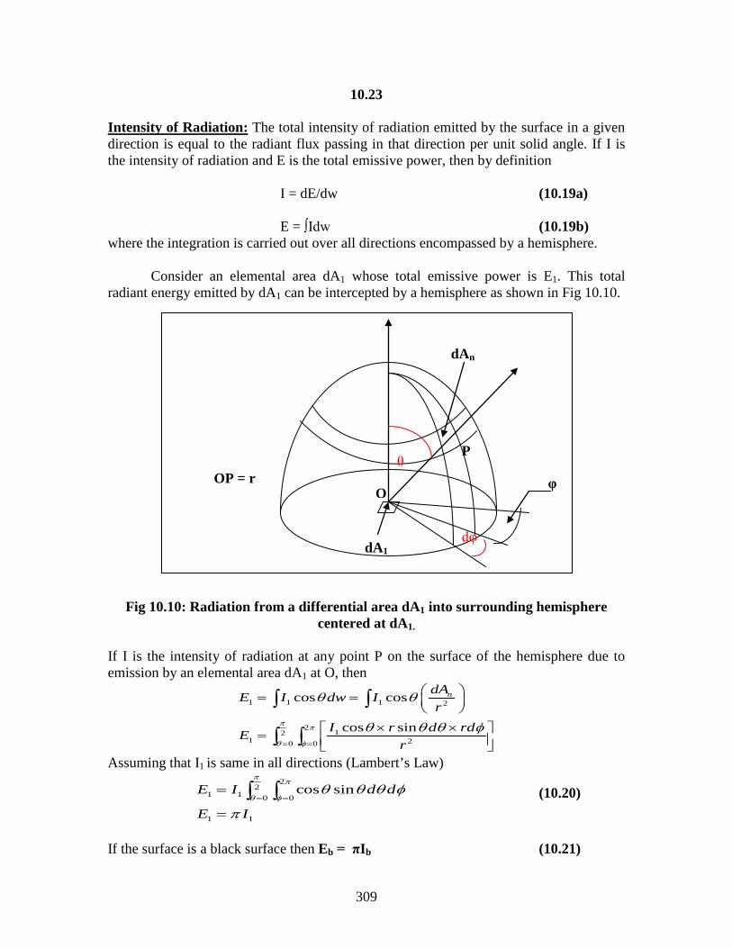
309
10.23 Intensity of Radiation: The total intensity of radiation emitted by the surface in a given direction is equal to the radiant flux passing in that direction per unit solid angle. If I is the intensity of radiation and E is the total emissive power, then by definition
I = dE/dw (10.19a) E = ∫Idw (10.19b)
where the integration is carried out over all directions encompassed by a hemisphere. Consider an elemental area dA1 whose total emissive power is E1. This total radiant energy emitted by dA1 can be intercepted by a hemisphere as shown in Fig 10.10.
Fig 10.10: Radiation from a differential area dA1 into surrounding hemisphere centered at dA1.
If I is the intensity of radiation at any point P on the surface of the hemisphere due to emission by an elemental area dA1 at O, then
1 1 1 2
212
1 20 0
cos cos
cos sin
ndAE I dw Ir
I r d rdEr
π π
θ φ
θ θ
θ θ θ φ= =
= =
× × =
∫ ∫
∫ ∫
Assuming that I1 is same in all directions (Lambert’s Law) 2
21 1 0 0
1 1
cos sinE I d d
E I
π π
θ φθ θ θ φ
π= =
=
=
∫ ∫ (10.20)
If the surface is a black surface then Eb = πIb (10.21)
O
P
dA1
dAn
φ θ
dφ
OP = r
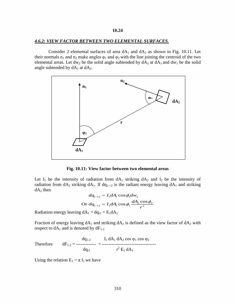
310
10.24 4.6.2: VIEW FACTOR BETWEEN TWO ELEMENTAL SURFACES. Consider 2 elemental surfaces of area dA1 and dA2 as shown in Fig. 10.11. Let their normals n1 and n2 make angles φ1 and φ2 with the line joining the centroid of the two elemental areas. Let dw2 be the solid angle subtended by dA2 at dA1 and dw1 be the solid angle subtended by dA1 at dA2.
Fig. 10.11: View factor between two elemental areas Let I1 be the intensity of radiation from dA1 striking dA2 and I2 be the intensity of radiation from dA2 striking dA1. If dq1->2 is the radiant energy leaving dA1 and striking dA2 then
1 2 1 1 1 2
2 21 2 1 1 1 2
coscosOr cos
dq I dA dwdAdq I dA
r
φφφ
→
→
=
=
Radiation energy leaving dA1 = dqr1 = E1dA1 Fraction of energy leaving dA1 and striking dA2 is defined as the view factor of dA2 with respect to dA1 and is denoted by dF1-2 dq1-2 I1 dA1 dA2 cos φ1 cos φ2 Therefore dF1-2 = ------------- = ----------------------------------- dqr1 r2 E1 dA1 Using the relation E1 = π I1 we have
n1
n2
φ1
φ2
dA1
dA2
r
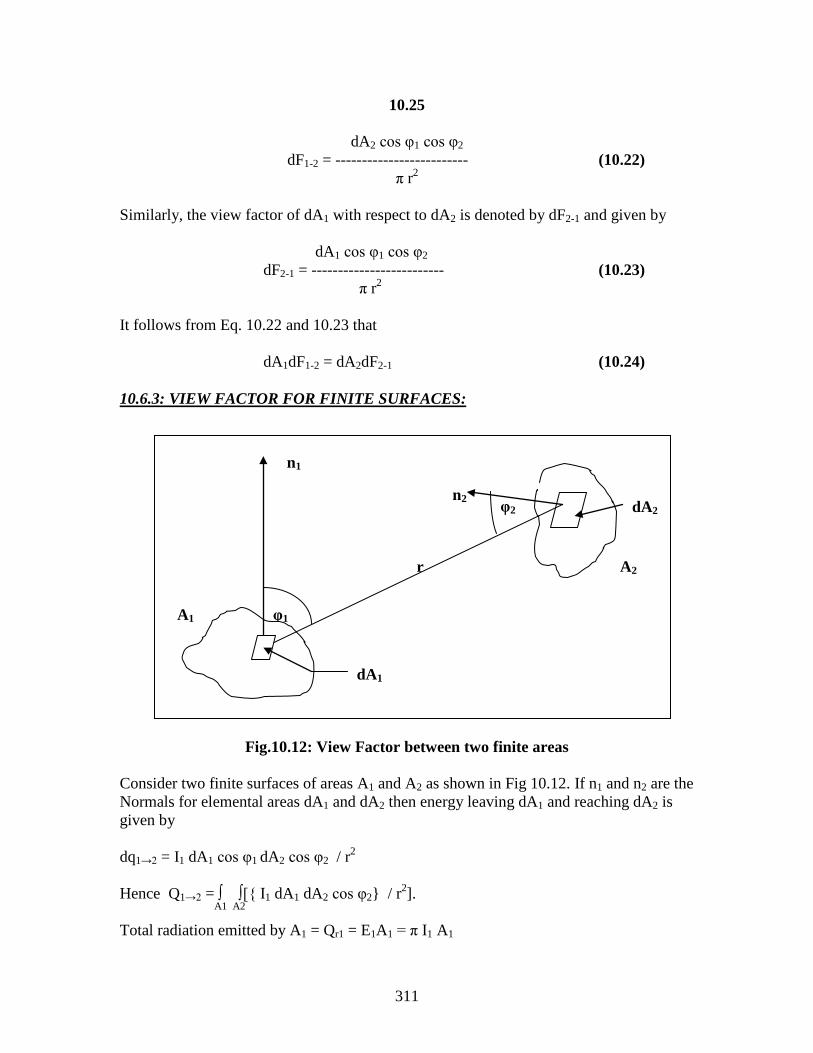
311
10.25
dA2 cos φ1 cos φ2 dF1-2 = ------------------------- (10.22)
π r2 Similarly, the view factor of dA1 with respect to dA2 is denoted by dF2-1 and given by dA1 cos φ1 cos φ2
dF2-1 = ------------------------- (10.23) π r2
It follows from Eq. 10.22 and 10.23 that
dA1dF1-2 = dA2dF2-1 (10.24)
10.6.3: VIEW FACTOR FOR FINITE SURFACES:
Fig.10.12: View Factor between two finite areas
Consider two finite surfaces of areas A1 and A2 as shown in Fig 10.12. If n1 and n2 are the Normals for elemental areas dA1 and dA2 then energy leaving dA1 and reaching dA2 is given by dq1→2 = I1 dA1 cos φ1 dA2 cos φ2 / r2 Hence Q1→2 = ∫ ∫[{ I1 dA1 dA2 cos φ2} / r2]. A1 A2
Total radiation emitted by A1 = Qr1 = E1A1 = π I1 A1
n1
n2
dA1
r
dA2
φ1
φ2
A1
A2
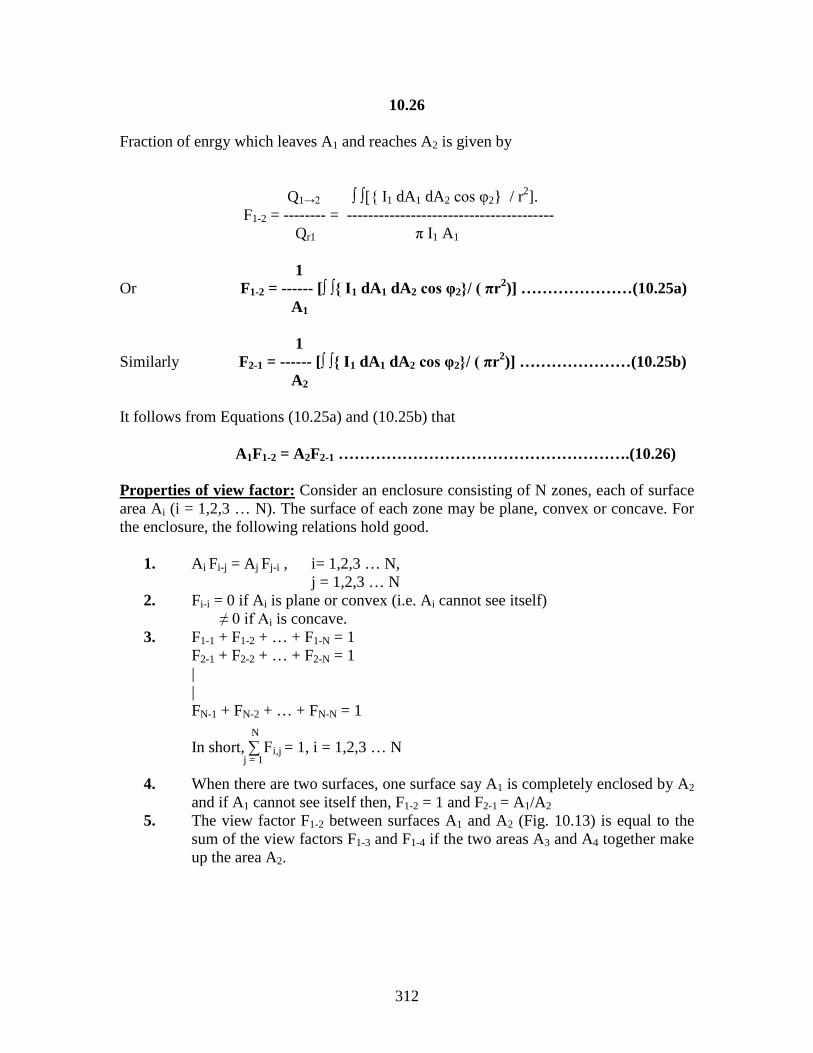
312
10.26 Fraction of enrgy which leaves A1 and reaches A2 is given by Q1→2 ∫ ∫[{ I1 dA1 dA2 cos φ2} / r2]. F1-2 = -------- = --------------------------------------- Qr1 π I1 A1 1 Or F1-2 = ------ [∫ ∫{ I1 dA1 dA2 cos φ2}/ ( πr2)] …………………(10.25a) A1
1 Similarly F2-1 = ------ [∫ ∫{ I1 dA1 dA2 cos φ2}/ ( πr2)] …………………(10.25b) A2
It follows from Equations (10.25a) and (10.25b) that A1F1-2 = A2F2-1 ……………………………………………….(10.26) Properties of view factor: Consider an enclosure consisting of N zones, each of surface area Ai (i = 1,2,3 … N). The surface of each zone may be plane, convex or concave. For the enclosure, the following relations hold good.
1. Ai Fi-j = Aj Fj-i , i= 1,2,3 … N, j = 1,2,3 … N
2. Fi-i = 0 if Ai is plane or convex (i.e. Ai cannot see itself) ≠ 0 if Ai is concave.
3. F1-1 + F1-2 + … + F1-N = 1 F2-1 + F2-2 + … + F2-N = 1 | | FN-1 + FN-2 + … + FN-N = 1 N In short, ∑ Fi,j = 1, i = 1,2,3 … N j = 1
4. When there are two surfaces, one surface say A1 is completely enclosed by A2 and if A1 cannot see itself then, F1-2 = 1 and F2-1 = A1/A2
5. The view factor F1-2 between surfaces A1 and A2 (Fig. 10.13) is equal to the sum of the view factors F1-3 and F1-4 if the two areas A3 and A4 together make up the area A2.

313
10.27
Fig. 10.13 : Additive relation between view factors i.e., F1-2 = F1-3 + F1-4 . It should however be noted that F2-1 ≠ F3-1 + F3-4 View factors for standard configurations: The determination of view factors has been the object of considerable research. In cases where the integrals in Eq. 10.25 and Eq. 10.26 cannot be solved analytically, numerical methods have been used. Some of these results are represented graphically for certain standard configurations like
(i) Shape factors between parallel rectangles of equal size. (ii) Shape factors between rectangles perpendicular to each other and having a
common edge (iii) Shape factor from an elemental area dA1 to a rectangular area A2 (iv) Shape factor between two coaxial parallel discs (v) Shape factors for concentric cylinders of finite length etc.
With the help of those charts and View Factor algebra, shape factors between surfaces not covered above can be determined. 10.7 ILLUSTRATIVE EXAMPLES ON VIEW FACTORS: Example 10.11: Determine the view factor between an elemental area A1 and a circular disc A2 of radius R. The two areas are parallel to each other and positioned at a distance L form each other such that the perpendicular to A1 passes through the centre of A2.
A1
A3 A4
A2 = A3 + A4

314
10.28
Fig.E10.11: Figure for example 10.11
( ) ( )
1 2
2
1 2 1 21 1 2 2
1 2 1 2
2 22
1 1 2 1 1 22 20
2 21 2 2
22
1 2 2 2 2 20
cos cos
Since and , the above exp can be written as
cos 2 cos
Now cos cos and
2
A A
R
A
R
dA dAA Fr
A A
dA dA F A Fr r
L r LL
d LF LL L
φ φπ
φ φ φ
φ πρ ρ φπ π
φ φ ρρ
πρ ρρ π ρ
−
− −
−
=
<< = =
= ⇒ =
= = = ++
∴ = =+ +
∫ ∫
∫ ∫
∫ ( )22 20
22
1 2 2 2
2
sin
R d
L
RFL R
ρ ρρ
α−
+
∴ = =+
∫
Example 10.12: Obtain an expression for the shape factor for a conical cavity with respect to itself. The height of the cavity is H and the semi vertex angle of the cavity is α (See Fig. E10.12a) Solution:
R ρ
r L
α
Φ2
Φ1

315
10.29
Refering to Fig. 10.12(b) we have A1 and A2 form an enclosure. Hence F1-1 + F1-2 = 1, and F2-1 + F2-2 = 1. Since A2 cannot see itself, F2-2 = 0. Hence F2-1 = 1.0 But A1F1-2 = A2F2-1. Therefore F1-2 = A2 / A1.
___________ From Fig. E10.12(b), dA1 = 2π r ds = 2 π √ (dr2 + dz2) ____________ Or dA1 = 2 π z tan α dz √ [(dr / dz)2 + 1] _______________ = 2 π z tan α dz √ [ tan 2 α + 1 ] = 2 π z dz tan α sec α H Therefore A1 = ∫2 π z dz tan α sec α = πH2 tan α sec α 0
πH 2 tan 2 α Hence F1-1 = 1 – F1-2 = 1 − ------------------------- = 1 – sin α πH2 tan α sec α Example 10.13: Consider 3 small surfaces each of area dA1 = dA2 = dA3 = 2 cm2 as shown in fig E10.13. (a) Calculate the solid angle subtended by dA2 with respect to a point on dA1 (b) The solid angle subtended by dA3 with respect to a point on dA1 and (c) The elemental Diffuse factors dFdA1-dA2 and dFdA1-dA3.
H α
Fig. E10.12(a) : Figure for Example 10.12
dz
A2
z
r ds
Fig. E10.12 (b):

316
10.30
1 2
2 1 2 10
52 22 1 2 2
12
03 33 1 32
13
533 1 2 2
13
2
If is the solid angle subtended by w.r.t a point on then
cos 2cos 45 1.57 10 sr300
cosSimilarly (but 0 )
2 5 10 sr200
cosdA dA
dw dA dAdAdw
rdAdw
rdAdwrdAdF
φ
φ φ
φ
−
−−
−
−−
−
= = = ×
= =
∴ = = = ×
=( )
1 3
0 0612 2
2212
2 053 13 3
2 213
cos 2 cos30 cos 45 4.33 10300
cos cos 2 cos 0Similarly 1.59 10200dA dA
r
dAdFr
φππ
φ φπ π
−
−−
× ×= = ×
×
×= = = ×
×
Example 10.14: Determine the view factor F1-2 between an elemental surface dA1 and the finite rectangular surface A2 for the geometric arrangements shown in Fig E10.14
dA2
dA3
dA1
n2 n3
n1
Φ2
Φ1
r13
r12
Φ1 = 30 0; Φ2 = 45 0 ; r12 = 300 cm ; r13 = 200 cm ; dA1 = dA2 = dA3 = 2 cm2 ;
Fig. E10.13: Figure for example 10.13

317
10.31
Soluiton : (a) The configuration in Fig. E10.14(a) is a standard configuration for which the analytical expression for F1-2 is given by 1 x y y x F1-2 = ---- [ ------------ tan − 1 {------------- } + ------------- tan − 1 { ----------------} ] 2π √(1 + x2) √(1 + x2) √(1 + y2) √(1 + y2) Where x = L1 / D = 3 / 3 = 1 ; and y = L2 / D = 4 / 3 = 1.33 Substituting these values in the expression for F1-2 we get 1 1 1.33 1.33 1 F1-2 = ---- [ ------------ tan − 1 {------------- } + ------------- tan − 1 { ----------------} ] 2π √(1 + 12) √(1 + 12) √(1 + 1.332) √(1 + 1.332) Or F1-2 = 0.154 (a) The area A2 is divided into two equal areas A3 and A4 both having the common edge of width L1 = 3 m.Then F1-2 = F1-3 + F1-4 = 2 F1-3 (Because F1-3 = F1-4) = 2 x 0.15 v4 = 0.308
4 m
A2 A2
A2
8 m 8 m
4 m 4 m
3 m 3 m
3 m
3 m
6 m
3 m
(a) (b) (c) Fig. E10.14: Figures for example 10.14

318
10.32
(c) In this case A2 is divided into three equal areas A3,A4, and A5 as shown below
Example 10.15: Determine the Shape factor F1-2 for the configuration shown in Fig E10.15 Solution:
A3
A4 A5
Now F1-2 = F1-3 + F1-4 + F1-5 = 3 F1-3 = 3 x 0.154 = 0.462
A1
A2
1 m
1 m
3 m
1 m 1 m
Fig. E10.15: Figure for example 10.15

319
10.33 A6 F6-1 A4 F4-1 F1-2 = F1-6 − F1-4
= ---------- − -------------- A1 A1
A6 A4 = ------ [ F6-5 − F6-3 ] − ---------- [ F4-5 − F4-3 ] A1 A1
Values of F6-5, F6-3, F4-5 and F4-3 can be obtained from chart as follows.
To find F6-5:
Example 10.16: Find F1-2 for the configuration shown in Fig. E10.16
3 m
2 m
2 m
A5
A6
A5 = A6 = 3 x 2 = 6 m 2 ; L1 / W = L2/W = 2/3 = 0.667; From chart F6-5 = 0.22. Similarly we Get F6-3 = 0.16; F4-5 = 0.32 ; F4-3 = 0.27
6 3 x 1 Hence F1-2 = ------- [ 0.22 − 0.16 ] − ------- [ 0.32 − 0.27 ] 1 x 3 3 x 1 Thus F1-2 = 0.07
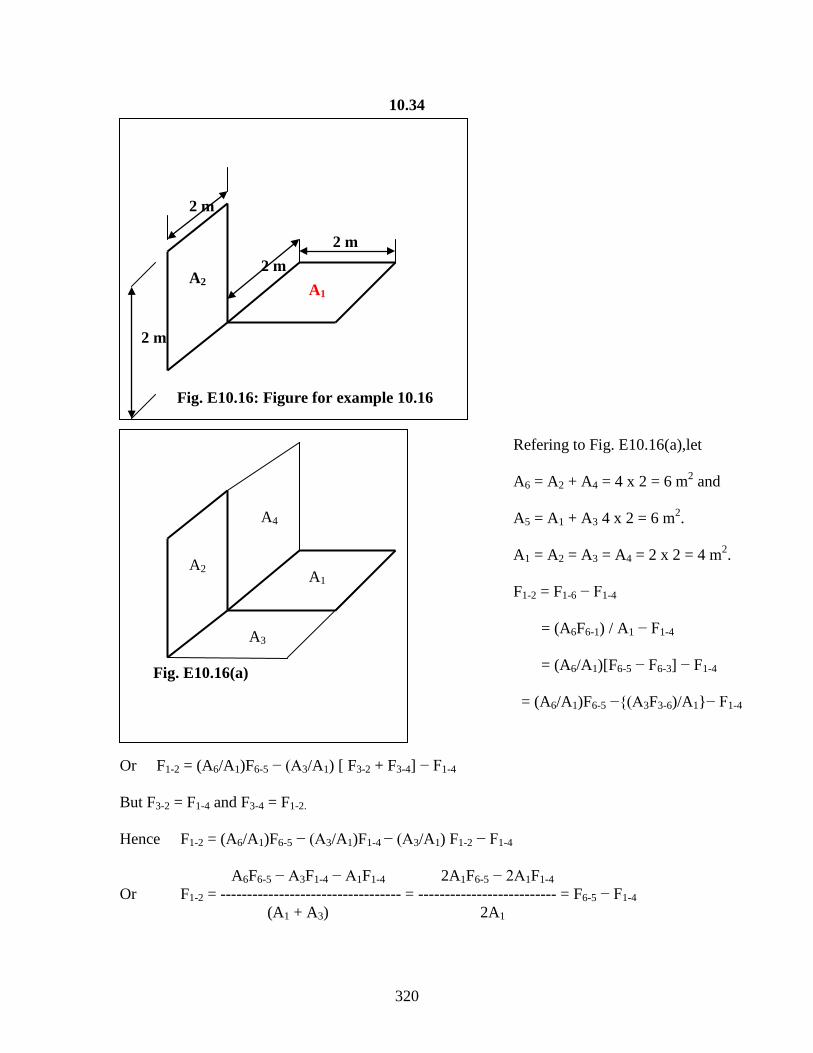
320
10.34
Or F1-2 = (A6/A1)F6-5 − (A3/A1) [ F3-2 + F3-4] − F1-4 But F3-2 = F1-4 and F3-4 = F1-2.
Hence F1-2 = (A6/A1)F6-5 − (A3/A1)F1-4 − (A3/A1) F1-2 − F1-4 A6F6-5 − A3F1-4 − A1F1-4 2A1F6-5 − 2A1F1-4 Or F1-2 = ---------------------------------- = -------------------------- = F6-5 − F1-4 (A1 + A3) 2A1
2 m
2 m
2 m 2 m
A1 A2
Fig. E10.16: Figure for example 10.16
A1 A2
A3
A4
Fig. E10.16(a)
Refering to Fig. E10.16(a),let A6 = A2 + A4 = 4 x 2 = 6 m2 and A5 = A1 + A3 4 x 2 = 6 m2. A1 = A2 = A3 = A4 = 2 x 2 = 4 m2. F1-2 = F1-6 − F1-4 = (A6F6-1) / A1 − F1-4
= (A6/A1)[F6-5 − F6-3] − F1-4 = (A6/A1)F6-5 −{(A3F3-6)/A1}− F1-4

321
10.35
To find F6-5:- L2 = L1 = 2 m; W = 4 m. L1 / W = L2 / W = 2 / 4 = 0.5. From chart F5-6 = 0.25 = F6-5 since A5 = A6. Similarly F1-4 = 0.2. Hence F1-2 = 0.25 – 0.20 = 0.05 Example 10.17: Find the Shape Factor F2-1 for the configuration shown in fig E10.17
Solution: Refer to Fig. 10.17 (a) F2-1 = F2-3 + F2-5 = F2-3 + (A5 F5-2) / A2 = F2-3 + (A5 / A2) [ F5-6 – F5-4] = F2-3 + (A6F6-5) / A2 − (A5F5-4) / A2 = F2-3 + (A6 / A2) [F6-1 − F6-3] − (A5F5-4) / A2 = F2-3 + (A6 / A2)F6-1 − (A3F3-6) / A2 − (A5F5-4) / A2 = F2-3 + (A6 / A2)F6-1 − (A3F2-1) / A2 − (A5F5-4) / A2 Or [( 1 + (A3 / A2) ] F2-1 = F2-3 + (A6 / A2)F6-1 − (A5F5-4) / A2
A1
A2
0.5 2 m
2 m
2 m
Fig. E10.17: Figure for example 10.17

322
10.36
F2-3 + (A6 / A2)F6-1 − (A5F5-4) / A2 Or F2-1 = ----------------------------------------------------- [( 1 + (A3 / A2) ] From chart : F2-3 = 0.06 ; F5-4 = 0.17 ; F6-1 = 0.2 0.06 + 4 x 0.2 − 3 x 0.17 Hence F2-1 = --------------------------------- = 0.175 ( 1 + 1) Example 10.18: Find the Shape factor F1-2 for the configuration shown in Fig E10.18 Solution: Refer Fig. E10.18(a). F1-2 = F1-8 + F1-4 + F1-6. But F1-4 = F1-6. Hence F1-2 = F1-8 + 2F1-4 = F1-8 + 2 (A4F4-1) / A1 From example 10.16 we have F4-1 = F7-10 − F4-3
Hence F1-2 = F1-8 + 2 (A4 /A1) [F7-10 − F4-3] From chart F1-8 =0.15 ; F7-10 = 0.23 ; F4-3 = 0.2
A2
Fig. E10.17(a)
A4
A5 A3
A1 = A3 + A5; A6 = A2 + A4 A2 = A3 = 0.5 x 2 = 1 m 2 A4 = A5 = 1.5 x 2 = 3 m 2 A1 = A6 = 2 x 2 = 4 m2

323
10.37
a2
Hence F1-2 = 0.15 + 2 x -------------- x [0.23 – 0.20] = 0.27 [(a/2) x a]
A1
A2 a
a a/2
a Fig. E10.18: Figure for example 10.18
A1
A8
Fig. E10.18 (a)
A5
A6
A4
A3 A7 = A1 + A3 ; A10 = A4 + A8

324
`10.38 Example 10.19 A1 and A2 are two rectangular flat surfaces having a common edge and inclined at an arbitrary angle α to each other. They are very long along the common edge and have lengths of ab and ac respectively in the other direction. Show that F1-2 = (ab +ac) – bc 2ab Solution: Refer Fig. E10.19
Or F1-3 = (A3 / A1) – (A2F2-3) / A1 = (A3 / A1) – (A2 / A1) [1 – F2-1] = (A3 / A1) – (A2 / A1) + F1-2 Substituting this expression in Eq. (d) we get F1-2 = 1 – [(A3 / A1) – (A2 / A1) + F1-2] Solving for F1-2 we get (A1 + A2) – A3 (ab x 1) + (ac x 1) – (bc x 1) F1-2 = ---------------------- = ----------------------------------- 2A1 2 x (ab x 1) (ab + ac – bc) = ------------------- 2 ab
a b A1
c
A2 A3
A1,A2 and A3 form an enclosure. Hence F1-1 + F1-2 + F1-3 = 1. But F1-1 = 0. Hence F1-2 + F1-3 = 1 ………………….(a) similarly F2-1 + F2-3 = 1 ………………….(b) F3-1 + F3-2 = 1…………………..(c)
Fig. E10.19 From Eq. (a) we get F1-2 = 1 – F1-3 …...(d) From (c) we get F3-1 = 1 – F3-2 Or (A1F1-3) / A3 = 1 – (A2F2-3)/A3

325
10.39
Example 10.20: (Hottel’s cross string formula) Obtain an expression for the view factor between two flat surfaces, which extend to infinity in one direction. Solution: Refer Fig. E10.20
Fig. E10.20 : Figure for example 10.20 Consider unit width perpendicular to the plane of the paper. A1, A2, A3 and A4 form an enclosure. Hence we have F1-1 + F1-2 + F1-3 + F1-4 = 1 and F1-1 = 0. Therefore F1-2 + F1-3 + F1-4 = 1 …………………………(a) Similarly A1, A3 and A5 form an enclosure. Therefore we have F1-3 + F1-5 = 1 ………………………………..(b) Also F3-1 + F3-5 = 1 ………………………………..(c) and F5-1 + F5-3 = 1 ………………………………..(d) From Eq. (b) we have F1-3 = 1 – F1-5 = 1 – (A5F5-1) / A1
= 1 – (A5 / A1) [ 1 – F5-3] = 1 – (A5 / A1) + (A3F3-5) / A1
A1 = L1 x 1
A2 = L2 x 1
A4 = L4 x 1
A3 = L3 x 1
A6 = L6 x 1
A5 = L5 x 1

326
10.40
Or F1-3 = 1 – (A5 / A1) + (A3 / A1) [1 – F3-1] = 1 – (A5 / A1) + (A3 / A1) – F1-3 1 – (A5 / A1) + (A3 / A1) A1 – A5 + A3 Hence F1-3 = --------------------------------- = --------------------------- 2 2A1 A1 – A6 + A4 Similarly F1-4 = ------------------------ 2A1 Now from Eq. (a) we have F1-2 = 1 – [F1-3 + F1-4] Substituting the expressions obtained for F1-3 and F1-4 we get A1 – A5 + A3 A1 – A6 + A4 F1-2 = 1 – ------------------- − ------------------- 2A1 2A1 (A5 + A6) – (A3 + A4) (L5 + L6) – (L3 + L4) = ---------------------------- = ---------------------------- 2A1 2L1 Example 10.21: A truncated cone has top and bottom diameters of 10cm and 20cm and a height of 10cm. Calculate the shape factor between the top surface and the side and the side and itself. Solution: To find (i) F2-3 and (ii) F3-3 . Refer to Fig. E4.21.
(i) F2-1 = (A1F1-2) / A2. F1-2 can be directly obtained fom chart as follows:
L1 / r = 10 / 10 = 1 ; and L2 / r = 5 / 10 = 0.5. Hence fromchart F1-2 = 0.12. π x (10)2
Therefore F2-1 = -------------- x 0.12 = 0.48 π x (5)2 F2-3 = 1 – F2-1 = 1 – 0.48 = 0.52
(ii) F2-1 + F2-2 + F2-3 = 1 and F2-2 = 0.
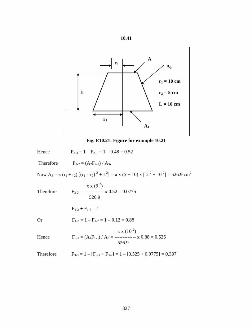
327
10.41
Fig. E10.21: Figure for example 10.21 Hence F2-3 = 1 – F2-1 = 1 – 0.48 = 0.52 Therefore F3-2 = (A2F2-3) / A3. Now A3 = π (r1 + r2) [(r1 – r2) 2 + L2] = π x (5 + 10) x [ 5 2 + 10 2] = 526.9 cm2 π x (5 2) Therefore F3-2 = ------------ x 0.52 = 0.0775 526.9 F1-2 + F1-3 = 1 Or F1-3 = 1 – F1-2 = 1 – 0.12 = 0.88 π x (10 2) Hence F3-1 = (A1F1-3) / A3 = ------------- x 0.88 = 0.525 526.9 Therefore F3-3 = 1 – [F3-1 + F3-2] = 1 – [0.525 + 0.0775] = 0.397
r2
r1
L
r1 = 10 cm r2 = 5 cm L = 10 cm
A1
A A3

328
10.42 Example 10.22: Determine the shape factors for the geometries shown in Fig. E10.23(a) to E10.23(i)
Fig. E 10.23 (a)
Long duct A1
A2
Find F1-2, F2-1 and F1-1
Long groove, A1 Surroundings, A2
Find F1-2, F2-1 and F1-1
Fig. E 10.23 (b)
2.0
1.0 A1 Surroundings, A3
Fig. E 10.23 (c)
Find F1-1 and F1-3
1.0
A1
Fig. E 10.23 (d)
A1 is covered by a hemispherical surface A2 of radius 1.5. Find F1-2, F1-3, F2-1 and F2-2

329
10.43
(e) F1-3 F2-3 F2-2 F2-1 F1-2 for disc (f) F1-2 F2-1 fro sphere on infinite surrounded by a short cylinder plane (g)F1-2 F2-1 F2-3 (h) F1-2 F2-1 F1-3 F2-3 (i) F1-2 F2-1 F1-1 F1-3 hemisphere 1 enclosing a small sphere 2 surrounded by a large enclosure 3
1.0
3.0
2.0
1
2
1
2
1.5 1.5
1.5
Surroundings 3
1.0 1
2
3
1.0 3.0

330
10.44 Solution:
( ) ( )
( )
1 1 1 2
2 1 2 2
2 2
2 1 1 1 2 2 2 1
2 21 2 2 1
1 1
1 1 1 2
1 and 2 form an enclosure11
since 2 is a flat surface, 01 but
2 1 12 1
1 11 1
F FF F
FF A F A F
A A RF FA A R
F F
π ππ
π π
− −
− −
−
− − −
− −
− −
∴ + =+ =
=
∴ = =×
∴ = = = =×
−∴ = − = − =
All the radiation from (1) which goes to the surroundings can be intercepted by an imaginary surface 21 as shown in Fig. Now 1 and 21 form an enclosure. Therefore from the above example
2 1 2 1 1 2 1 2 1 11 11; ; F F F F F ππ π′ ′− − − − −
−= = = = =
All the radiation from (1) which goes to the surroundings can be intercepted by an imaginary surface 2 and 4 as shown in Fig. Now, 1, 2 and 4 form an enclosure.
1 1 1 2 1 4
1 4 1 2
1but
F F FF F
− − −
− −
∴ + + ==
( ) ( )
1 1 1 2
2 1 2 2 2 4 2 2
2 1 2 4 2 1 2 4
2 4
2 12
2 2 11 2
1
1 2 ( )also 1 and 0
1 1from chart for two parallel coaxial discs 2 and 4
0.3831 0.383 0.617
1.00.617 0.62 2 1.0
F F aF F F F
F F F F
FF
A F RFA RL
ππ
− −
− − − −
− − − −
−
−
−−
∴ = − − − − − − − − − −+ + = =
∴ + = ⇒ = −
== − =
∴ = = × = ××
1 1
1 3 1 1
17 0.309
1 2 0.309 0.3831 1 0.383 0.617F
F F−
− −
=
∴ = − × == − = − =
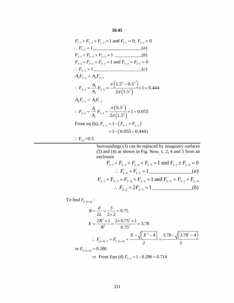
331
10.45
1 1 1 2 1 3 1 1 1 3
1 2
2 1 2 2 2 3
3 1 3 2 3 3 3 3 3 1
3 2
3 3 2 2 2 3
2 23
2 3 3 22
1 and 0; 01____________________( )
1 ___________( )1 and 0
1____________________( )
1.5 0.5
F F F F FF a
F F F bF F F F F
F cA F A F
AF FA
π
− − − − −
−
− − −
− − − − −
−
− −
− −
+ + = = =∴ =
+ + =+ + = = =
∴ ==
− ∴ = =( )
( )( )
( )( )
2
2 2 1 1 1 2
21
2 1 1 2 22
2 2 2 1 2 3
2-2
1 0.4442 1.5
0.51 0.055
2 1.5
From eq (b), 1
1 0.055 0.444F =0.5
A F A F
AF FA
F F F
π
π
π
− −
− −
− − −
× =
=
∴ = = × =
= − +
= − +
∴ Surroundings (3) can be replaced by imaginary surfaces (5) and (4) as shown in Fig. Now, 1, 2, 4 and 5 form an enclosure
1 1 1 2 1 4 1 5 1 1 1 4
1 2 1 5
2 1 2 2 2 4 2 5 2 5 2 1 2 4
2 2 2 5
1 and 01________________( )
1 and 2 1_______________( )
F F F F F FF F a
F F F F F F FF F b
− − − − − −
− −
− − − − − − −
− −
+ + + = ± =∴ + =
+ + + = = +∴ + =
( )
( ) ( )
( )
5 1 4
2 2
2 2
2 2
1 4 5 5 1 4
5 1 4
5 2
To find :
3 0.752 2 22 1 2 0.75 1 3.78
0.75
4 3.78 3.78 4
2 2or 0.286
From Eqn (d) 1 0.286 0.714
F
dRLRXR
X XF F
F
F
− +
+ − − +
− +
−
= = =×
+ × += = =
− − − − ∴ = = =
=
⇒ = − =

332
10.46
( )
( ) ( )
( )( )
( )( )
25 5 2
2 52
2 2
1 1 55 4 5 15 1 4 5 1 4
5
2
2
25 5 4
4 5 2 24
4 2
1.50.714 0.268
2 1.5 2From (b) 1 2 0.268 0.465
Now
0.50.286 0.35 0.247
1.5
1.50.247 0.278
1.5 0.5
From (c) 1 0.278 0.
A FFAF
A FF F F FA
A FFA
F
π
π
π
π
π
π
−−
−
−− −− + − +
−−
−
∴ = = × =× ×
∴ = − × =
= − = −
= − × =
∴ = = × =−
= − =
( )
( )
2 24 4 2
2 42
2 1 2 5 2 4
2 1
2 3 2 5 2 52 1 4
2 3
722
1.5 0.50.722 0.24
2 1.5 20.268 0.240
0.0282 2 0.268
0.536
A FFA
F F FF
F F F F
F
π
π−
−
− − −
−
− − −− +
−
−∴ = = × =
× ×= − = −∴ == + = = ×
∴ =
10.8 RADIATION HEAT EXCHANGE BETWEEN FINITE SURFACES 10.8.1 RADIATION HEAT EXCHANGE BETWEEN FINITE BLACK SURFACES Consider two black surfaces of area A1 and A2 and at temperatures T1 and T2 as shown in Fig 10.14. Then radiation leaving A1 and reaching A2 can be written as
Fig 10.14: Radiation between two Finite Block Surfaces.
A1,T1
A2,T2

333
10.47
Q1->2 = A1 J1 F1-2 Since A1 is a black surface, J1 = Eb1 thus,
Q1->2 = A1 Eb1 F1-2 Similarly radiation leaving A2 and reaching A1 is given by
Q2->1 = A2 Eb2 F2-1 Net heat exchange between A1 and A2 can be written as
Q12 = Q1->2 – Q2->1 = A1 F1-2 Eb1 – A2 F2-1 Eb2 But, A1 F1-2 = A2 F2-1 Thus, Q1-2 = A1F1-2 (Eb1 – Eb2)
Q1-2 = σA1F1-2(T14
– T24) -----------------(10.27)
10.8.2 RADIATION HEAT EXCHANGE BETWEEN FINITE GREY SURFACES (NET WORK METHOD) The calculation of radiation heat transfer between black surfaces is relatively easy because all the radiant energy which strikes a surface is absorbed by it. When non black bodies are involved, the situation is much more complex because all the energy striking a surface will not be absorbed: part will be reflected back to another heat transfer surface, and part may be reflected out of the system entirely. The problem can become complicated because the radiant energy can be reflected back and forth between heat transfer surfaces several times. While deriving the expression for radiation exchange between any two finite grey surfaces the following assumptions are made
i. All the surfaces are diffuse and uniform in temperature. ii. The reflection and emissive properties are constant over all the surface
iii. Radiosity and irradiation are uniform over each surface. This assumption is not strictly correct even for ideal grey diffuse surfaces, but the problems become exceedingly complex when this restriction is not imposed.
iv. The surfaces are opaque (i.e. Transmissivity is zero) Now the net radiation from a surface is given by

334
10.48
( )( )
( )
( )
( )( ) ( )
but 1
assuming , 1
or 1
11 1
________________________ 4.2811
r
b
b
bbr
b b br
Q A J G
J E G
J E GJ EG
J J EJ EQ A J A
A E J E J E JQR
A
α
α ε ε εεε
ε εεε ε
εεε
ε
= −
= + −
= = + −
−=
−− − + − ∴ = − = − −
− − −= = =
−−
Eq. 4.28 can be interpreted as follows… (Eb-J) can be thought of as thermal potential, R = (1-ε)/εA can be thought of as thermal resistance offered by the surface for radiation, as Qr is the radiation heat flow rate. Therefore a radiating surface can be replaced by an element as shown in Fig 10.15
Fig 10.15: Element representing surface resistance in the Radiation network method Now let us consider the radiation heat exchange between two surfaces A1 and A2. Radiation which leaves A1 and strikes A2 is given by
1 2 1 1 1 2Q A J F→ −= Similarly Radiation which leaves A2 and strikes A1 is given by
2 1 2 2 2 1Q A J F→ −= Therefore net radiation heat transfer from A1 to A2 is given by
Qr Eb J
1-ε R = ----------
Aε
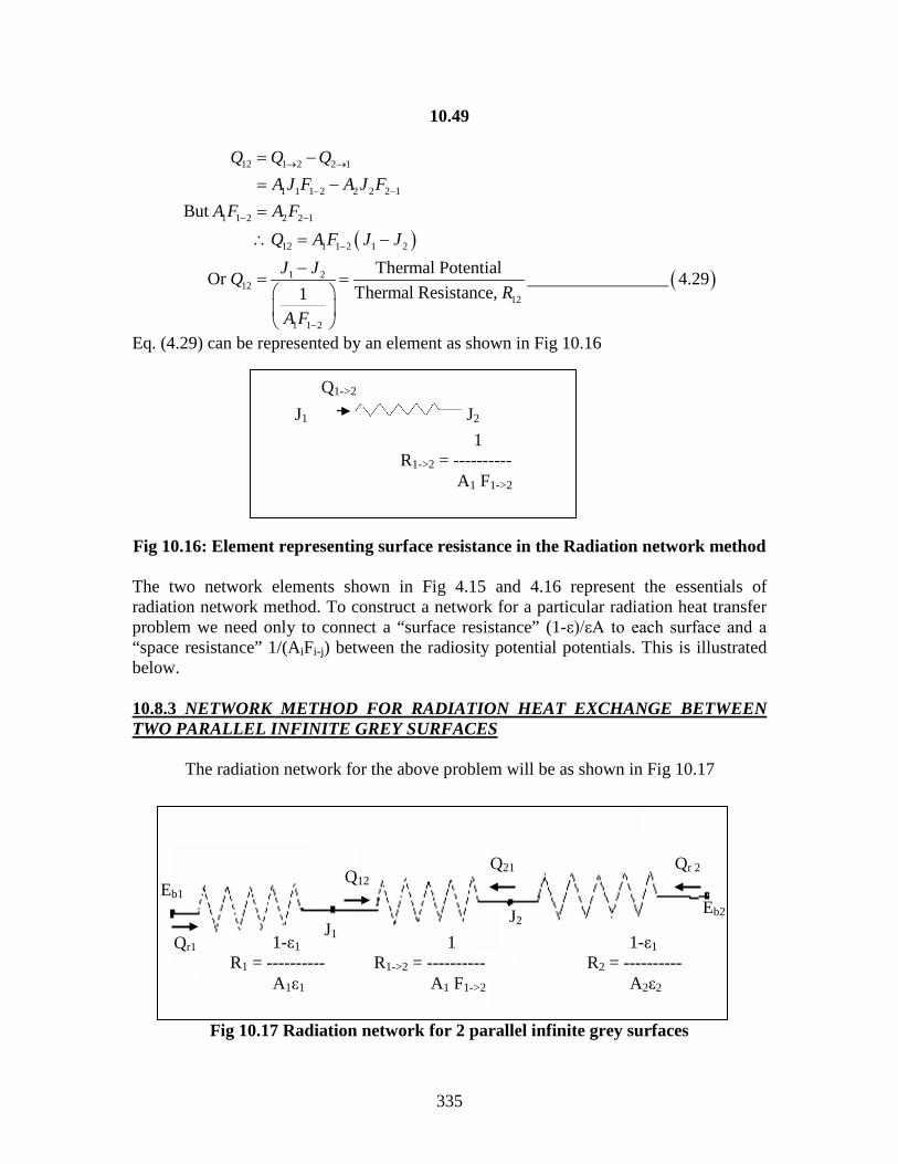
335
10.49
( )
( )
12 1 2 2 1
1 1 1 2 2 2 2 1
1 1 2 2 2 1
12 1 1 2 1 2
1 212
12
1 1 2
But
Thermal PotentialOr ________________ 4.29Thermal Resistance, 1
Q Q QA J F A J F
A F A FQ A F J J
J JQR
A F
→ →
− −
− −
−
−
= −= −=
∴ = −
−= =
Eq. (4.29) can be represented by an element as shown in Fig 10.16 Fig 10.16: Element representing surface resistance in the Radiation network method The two network elements shown in Fig 4.15 and 4.16 represent the essentials of radiation network method. To construct a network for a particular radiation heat transfer problem we need only to connect a “surface resistance” (1-ε)/εA to each surface and a “space resistance” 1/(AiFi-j) between the radiosity potential potentials. This is illustrated below. 10.8.3 NETWORK METHOD FOR RADIATION HEAT EXCHANGE BETWEEN TWO PARALLEL INFINITE GREY SURFACES The radiation network for the above problem will be as shown in Fig 10.17
Fig 10.17 Radiation network for 2 parallel infinite grey surfaces
Q1->2 J1 J2
1 R1->2 = ---------- A1 F1->2
Qr1 1-ε1 R1 = ----------
A1ε1
1-ε1 R2 = ----------
A2ε2
1 R1->2 = ---------- A1 F1->2
Qr 2 Q21 Q12
J1 J2
Eb1 Eb2
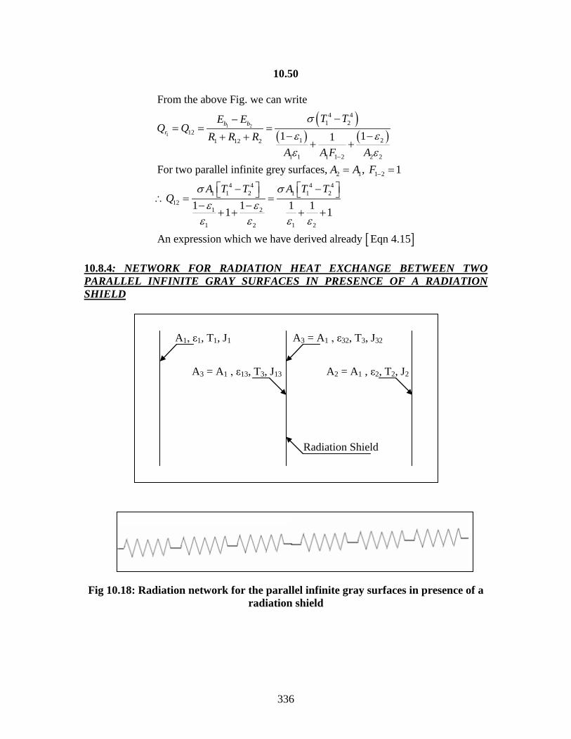
336
10.50
( )( ) ( )
1 2
1
4 41 2
121 21 12 2
1 1 1 1 2 2 2
2 1 1 2
4 4 4 41 1 2 1 1 2
121 2
1 21 2
From the above Fig. we can write
1 11
For two parallel infinite grey surfaces, , 1
1 1 1 11
b br
T TE EQ Q
R R RA A F A
A A F
A T T A T TQ
σε εε ε
σ σε ε
ε εε ε
−
−
−−= = =
− −+ ++ +
= =
− − ∴ = =− −
++ +
[ ]
1
An expression which we have derived already Eqn 4.15
+
10.8.4: NETWORK FOR RADIATION HEAT EXCHANGE BETWEEN TWO PARALLEL INFINITE GRAY SURFACES IN PRESENCE OF A RADIATION SHIELD
Fig 10.18: Radiation network for the parallel infinite gray surfaces in presence of a
radiation shield
A1, ε1, T1, J1
A2 = A1 , ε2, T2, J2 A3 = A1 , ε13, T3, J13
A3 = A1 , ε32, T3, J32
Radiation Shield

337
10.51
From Fig 10.18 the net radiation heat transfer from A1 to A2 is given
by
1 212
1 13 3 3 32 2
4 41 2
13 321 2
1 1 1 13 3 13 3 32 3 32 2 2
13 32 1 2 3
4 41 1 2
1213 321 2
1 13 32 2
4 41 1 2
12
1 2
1 11 11 1
But 1;
1 11 11 1
1 1
b bE EQ
R R R R R R
T T
A A F A A A F AF F A A A
A T TQ
A T TQ
σε εε ε
ε ε ε ε
σε εε ε
ε ε ε ε
σ
ε ε
′
−=
+ + + + +
− =− −− −
+ + + + +
= = = =
− ∴ =− −− −
+ + + + +
− =+ −
( )
13 32
________________ 4.301 11 1
ε ε
+ + −
10.8.5: RADIATION NETWORK FOR HEAT EXCHANGE BETWEEN TWO SURFACES, ONE SURFACE COMPLETELY ENCLOSING THE OTHER (The enclosed surface cannot see itself)
1 1 1 2 1 1
1 2
11 1 2 2 2 1 2 1
2
1 and 01
F F FF
AA F A F FA
− − −
−
− − −
+ = =∴ =
= ⇒ =
( )
1 2
1
4 41 2
121 21 12 2
1 2 1 1 2 2 2
4 41 1 2
121
1 2 2
1 11
__________________ 4.311 1 1
b br
T TE EQ Q
R R RA A F A
A T TQ
AA
σε εε ε
σ
ε ε
−
−− = = =− −+ + + +
− ∴ =
+ −
A1, ε1, T1
A2, ε2, T2
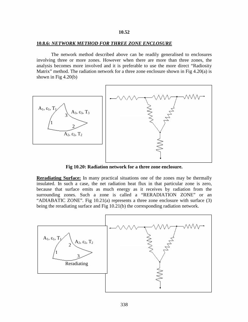
338
10.52 10.8.6: NETWORK METHOD FOR THREE ZONE ENCLOSURE The network method described above can be readily generalised to enclosures involving three or more zones. However when there are more than three zones, the analysis becomes more involved and it is preferable to use the more direct “Radiosity Matrix” method. The radiation network for a three zone enclosure shown in Fig 4.20(a) is shown in Fig 4.20(b)
Fig 10.20: Radiation network for a three zone enclosure. Reradiating Surface: In many practical situations one of the zones may be thermally insulated. In such a case, the net radiation heat flux in that particular zone is zero, because that surface emits as much energy as it receives by radiation from the surrounding zones. Such a zone is called a “RERADIATION ZONE” or an “ADIABATIC ZONE”. Fig 10.21(a) represents a three zone enclosure with surface (3) being the reradiating surface and Fig 10.21(b) the corresponding radiation network.
A1, ε1, T1
A2, ε2, T2
A3, ε3, T3
1 2
3
A1, ε1, T1 A2, ε2, T2
Reradiating
1 3
2
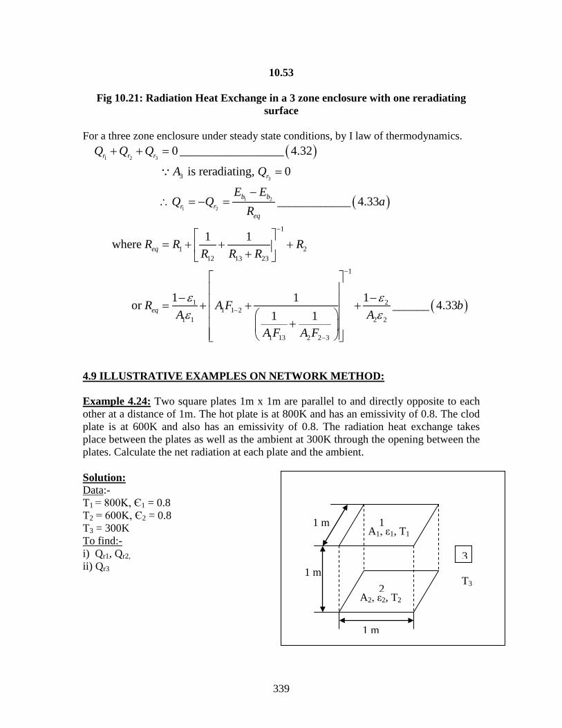
339
10.53
Fig 10.21: Radiation Heat Exchange in a 3 zone enclosure with one reradiating surface
For a three zone enclosure under steady state conditions, by I law of thermodynamics.
( )
( )
1 2 3
3
1 2
1 2
3
1
1 212 13 23
1
1 21 1 2
1 1 2
1 13 2 2 3
0 _________________ 4.32
is reradiating, 0
____________ 4.33
1 1where
1 11or 1 1
r r r
r
b br r
eq
eq
eq
Q Q Q
A Q
E EQ Q a
R
R R RR R R
R A FA A
A F A F
ε εε
−
−
−
−
+ + =
=
−∴ = − =
= + + + +
− − = + + +
+
( )2
______ 4.33bε
4.9 ILLUSTRATIVE EXAMPLES ON NETWORK METHOD: Example 4.24: Two square plates 1m x 1m are parallel to and directly opposite to each other at a distance of 1m. The hot plate is at 800K and has an emissivity of 0.8. The clod plate is at 600K and also has an emissivity of 0.8. The radiation heat exchange takes place between the plates as well as the ambient at 300K through the opening between the plates. Calculate the net radiation at each plate and the ambient. Solution: Data:- T1 = 800K, Є1 = 0.8 T2 = 600K, Є2 = 0.8 T3 = 300K To find:- i) Qr1, Qr2, ii) Qr3
1 m
1 m
1 m
1
2
A1, ε1, T1
A2, ε2, T2
3
T3

340
11
1 1
22
2 2
33 3 3
3 3
3
1 2 2 1
1 1 0.8 0.251 1 0.8
1 1 0.8 0.251 1 0.8
1 : is the area of the suroundings 1
0The radiation network for this problem will be as shown below
From chart 0
RA
RA
R A AA
R
F F
εεεε
εε
− −
− −= = =
× ×− −
= = =× ×
−= ∴
∴ =∴
= =
( )
( )
( )
1
2
1 1 1 2 1 3 1 1
1 3 1 2 2 3
121 1 2
131 1 3
231 2 3
4 8 4 2 21
4 8 42
.20But 1 and 0
1 1 0.2 0.81 1 5
1 1 0.21 1 1.25
1 1 0.81 1 1.25
1 1 0.8
5.67 10 800 23224 / 23.224 /
5.67 10 600 7b
b
F F F FF F F
RA F
RA F
RA F
E T W m KW m
E T
σ
σ
− − − −
− − −
−
−
−
−
−
+ + = =∴ = − = − = =
= = =×
= = =×
= = =×
= = × × = =
= = × × =
3
1
1
2 2
4 8 4 2 23
1 2 3
12 13
12 13
348 / 7.348 /
5.67 10 300 459 / 0.459 /
For steady state radiation, radiation energy cannot accumulate at nodes J , J and J
or 0
b
r
r
W m KW m
E T W m KW m
Q Q Q
Q Q Q
σ −
=
= = × × = =
∴ = +
− − =

341
( )
( ) ( ) ( )
( )
( ) ( ) ( )
1
2 2
32
1 1 2 1 3
1 12 13
1 2 11
21 23 21 23
22 2 1
2 12 23
2 1 22
0
0.45923.224or 0 _______0.25 5 1.25
similarly 0
0
0.4597.348 0 _______0.25 5 1.25
Solving Eqn (a) and
b
r r
bb
E J J J J JR R R
J J JJ a
Q Q Q Q Q Q
J EE J J JR R R
J J JJ b
− − −∴ − − =
− −−− − =
= + ⇒ − − =
−− −− − =
− −−− − =
[ ]
1
1
2
2
1 2 3 3 1 2
3
2 21 2
1
1
2
2
(b) simultaneously we get18.921 / ; 6.709 /
23.224 18.921 17.2120.25
7.348 6.709 2.5570.25
But 0 17.212 2.557
19.769
br
br
r r r r r r
r
J KW m J KW mE J
Q KWR
E JQ KW
R
Q Q Q Q Q Q
Q KW
= =− −
∴ = = =
− −= = =
+ + = ⇒ = − + = − + = −
Example 4.25 The configuration of a furnace can be approximated as an equilateral triangular duct which is sufficiently long that the end efforts are negligible. The hot wall is at 900K with an emissivity of 0.8 and the cold wall is at 400K with emissivity of 0.8. The third wall is a reradiating wall. Determine the net radiation flux leaving the hot wall. Solution: A1 = A2 = A3 = 1m2 (assumed) T1 =900K, Є1 = 0.8 T2 = 400K, Є2 = 0.8
A1, ε1, T1 A2, ε2, T2
600 600
A3, Reradiating Surface

342
10.56 The radiation network for the above problem will be as shown below
( ) ( )
11
1 1
22
2 2
1 2 31 2 1 3 2 3
1
12 23 131 1 2
1
1 212 13 23
1 1 0.8 0.251 0.8
1 1 0.8 0.251 0.8
Using Hottel's cross string formula, we have1 1 1
0.52 2 1
1 1 21 0.5
1 1
0.
eq
RA
RA
A A AF F F
A
R R RA F
R R RR R R
εεεε
− − −
−
−
− −= = =
×− −
= = =×
+ − + −= = = = =
×
∴ = = = = =×
= + + + +
=
( )1 2
1
1 2 3 3 2 1
1
4 4 8 4 41 2
2
2
1 125 0.25 1.8332 2 2
5.67 10 900 4001.833
19503 /0 and 0 19503 /
b br
eq eq
r r r r r r
T TE EQ
R R
W mQ Q Q Q Q Q W m
σ
−
−
+ + + = + − × × −− = = =
=
+ + = = ⇒ = − = −

343
10.57 Example 4.26 A short cylindrical enclosure is maintained at the temperatures as shown in Fig P4.26. Assuming Є2= Є3=1; Є1=0.8 determineQr1 and Qr2 Solution: From chart, F1-2 = 0.175 = F2-1 (A2=A1) Also, F1-1 + F1-2 + F1-3 = 1 and F1-1 = 0 So, F1-3 = 1 – F1-2 = 1 – 0.175 or
F1-3 = 0.825 = F2-3
The radiation network for the above problem will be as shown below
A1, ε1, T1 A2, ε2, T2
Reradiating Surface
1 m
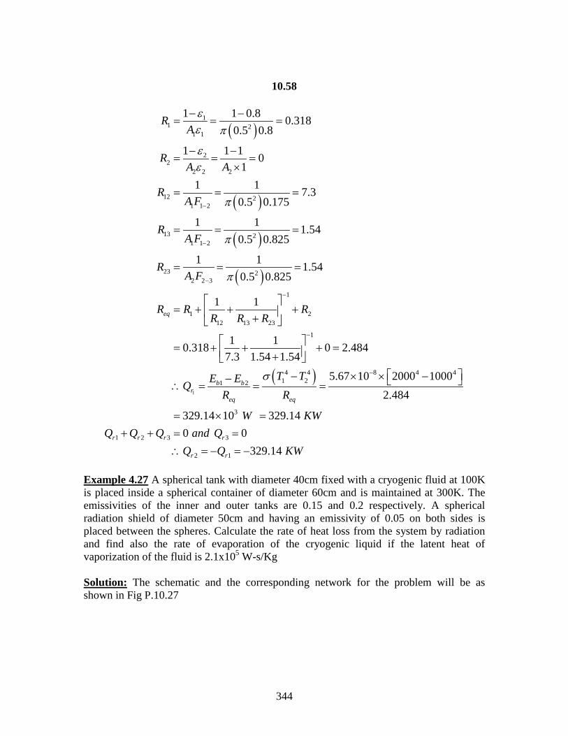
344
10.58
( )
( )
( )
( )
11 2
1 1
22
2 2 2
12 21 1 2
13 21 1 2
23 22 2 3
1
1 212 13 23
1
1 1 0.8 0.3180.5 0.8
1 1 1 01
1 1 7.30.5 0.175
1 1 1.540.5 0.825
1 1 1.540.5 0.825
1 1
1 10.318 0 27.3 1.54 1.54
eq
RA
RA A
RA F
RA F
RA F
R R RR R R
εε π
εε
π
π
π
−
−
−
−
−
− −= = =
− −= = =
×
= = =
= = =
= = =
= + + + +
= + + + = +
( )1
4 4 8 4 41 21 2
3
1 2 3 3
2 1
.484
5.67 10 2000 10002.484
329.14 10 329.14 0 0
329.14
b br
eq eq
r r r r
r r
T TE EQR R
W KWQ Q Q and Q
Q Q KW
σ − − × × −− ∴ = = =
= × =+ + = =
∴ = − = −
Example 4.27 A spherical tank with diameter 40cm fixed with a cryogenic fluid at 100K is placed inside a spherical container of diameter 60cm and is maintained at 300K. The emissivities of the inner and outer tanks are 0.15 and 0.2 respectively. A spherical radiation shield of diameter 50cm and having an emissivity of 0.05 on both sides is placed between the spheres. Calculate the rate of heat loss from the system by radiation and find also the rate of evaporation of the cryogenic liquid if the latent heat of vaporization of the fluid is 2.1x10⁵ W-s/Kg Solution: The schematic and the corresponding network for the problem will be as shown in Fig P.10.27
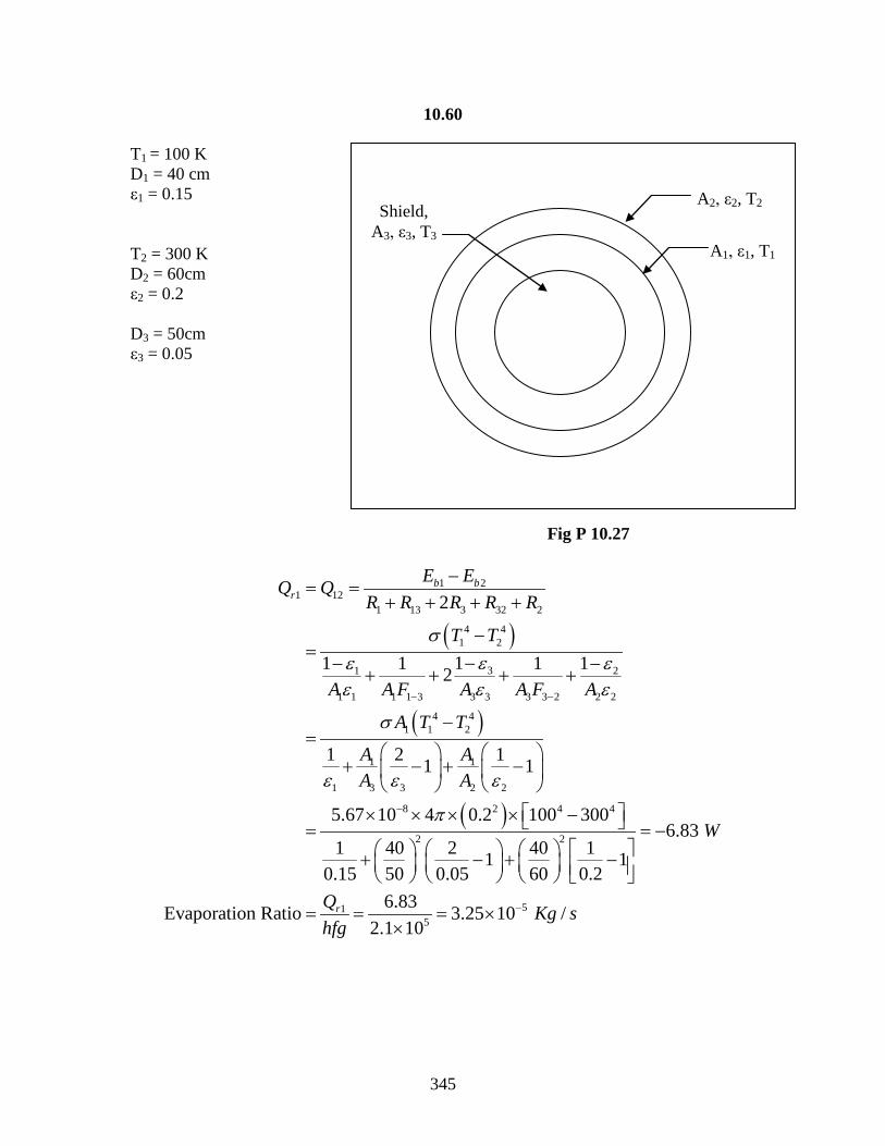
345
10.60 T1 = 100 K D1 = 40 cm ε1 = 0.15 T2 = 300 K D2 = 60cm ε2 = 0.2 D3 = 50cm ε3 = 0.05
Fig P 10.27
( )
( )
( )
1 21 12
1 13 3 32 2
4 41 2
31 2
1 1 1 1 3 3 3 3 3 2 2 2
4 41 1 2
1 1
1 3 3 2 2
8 2 4 4
2
2
11 11 12
1 2 11 1
5.67 10 4 0.2 100 300
1 40 2 4010.15 50 0.05 60
b br
E EQ QR R R R R
T T
A A F A A F A
A T T
A AA A
σεε ε
ε ε ε
σ
ε ε ε
π
− −
−
−= =
+ + + +
−=
−− −+ + + +
−=
+ − + −
× × × × − =
+ − +
2
515
6.83 1 1
0.26.83Evaporation Ratio 3.25 10 /
2.1 10r
W
Q Kg shfg
−
= − −
= = = ××
A1, ε1, T1
A2, ε2, T2 Shield, A3, ε3, T3

346
10.61 4.10 RADIOSITY- MATRIX METHOD FOR RADIATION IN ENCLOSURES The network method is quite easy to apply for determining the radiation exchange in enclosures having not more than 3 zones. As the number of zones forming the enclosure increases, the manipulations involved in the network method becomes enormous and the method is not so practical. Whereas the radiosity-matrix method is very straight forward and the method transforms the problem to the solution of an algebraic matrix equation for the unknown radiosities Ji [i=1,2,3,…….N] once these equations are solved for Ji then the net radiation flux or the zone temperature at any zone (i) can be immediately determined. This is illustrated below.
Consider an enclosure made up of N zones. Let Gi be the irradiation at zone i Let Ji be the Radiosity at zone i Net radiation heat flux from zone i is given by
( )_________ 4.34rii i i
i
Qq J GA
= = −
Radiation leaving and striking is given byj i
j i j j i j
i i j j
A AQ A F J
A F J− −
−
=
=
Zone i Ai, εi, Ti
Gi
Qri
Ji
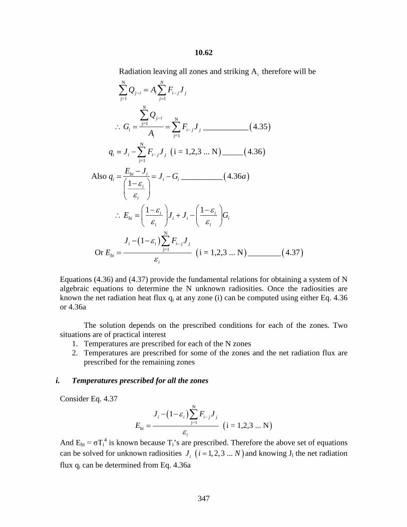
347
10.62
( )
( ) ( )
iN
j=1 1
Nj=1
j=1
N
j=1
Radiation leaving all zones and striking A therefore will be
___________ 4.35
i = 1,2,3 ... N _____ 4.36
Also 1
N
j i i i j jj
N
j i
i i j ji
i i i j j
bi ii i i
i
i
Q A F J
QG F J
A
q J F J
E Jq J Gε
ε
− −=
−
−
−
=
∴ = =
= −
−= = −
−
∑ ∑
∑∑
∑
( )
( )( ) ( )
N
j=1
__________ 4.36
1 1
1Or i = 1,2,3 ... N ________ 4.37
i ibi i i i
i i
i i i j j
bii
a
E J J G
J F JE
ε εε ε
ε
ε
−
− −∴ = + −
− −=
∑
Equations (4.36) and (4.37) provide the fundamental relations for obtaining a system of N algebraic equations to determine the N unknown radiosities. Once the radiosities are known the net radiation heat flux qi at any zone (i) can be computed using either Eq. 4.36 or 4.36a The solution depends on the prescribed conditions for each of the zones. Two situations are of practical interest
1. Temperatures are prescribed for each of the N zones 2. Temperatures are prescribed for some of the zones and the net radiation flux are
prescribed for the remaining zones
i. Temperatures prescribed for all the zones Consider Eq. 4.37
( )( )
N
j=11
i = 1,2,3 ... Ni i i j j
bii
J F JE
ε
ε
−− −=
∑
And Ebi = σTi4 is known because Ti’s are prescribed. Therefore the above set of equations
can be solved for unknown radiosities ( ) 1, 2,3 ... iJ i N= and knowing Ji the net radiation flux qi can be determined from Eq. 4.36a

348
10.63 Eq 4.37 can be rewritten as
( )
[ ]{ } { } ( )
[ ] ( )
{ }
N4
j=1
11 1N
N1 NN
1
2
N
1 _____________ 4.38
Equation (4.38) is of the form _________________________ 4.39
Where ___________ 4.39
____________
i ii j j i
i i
J F J T
M J T
m mM a
m m
JJ
J
J
ε σε ε −
−− =
=
= =
∑
( )
{ } ( )
[ ]( ) ( )
414
24
3
4N
ij
ij
ij
4.39
___________ 4.39
The elements of m of matrix M can be determined from
1______ 4.39
where 1 for i = j
0 for i j is known as KRONECKER del
ij i ijij
i
c
TT
T dT
T
Fm c
σσσ
σ
δ εε
δ
δ
=
− −=
=
= ≠
ta
ii. Temperature prescribed for some zones and net heat flux prescribed for others
In many practical situations, temperatures are prescribed for some of the zones and net heat fluxes for the remaining zones of an enclosure. In such problems we have to determine the net heat fluxes for the zones for which temperatures are specified and temperatures for the zones for which the net heat fluxes are prescribed. This can be done using the same equations (4.36) and (4.37) and illustrated below.
Let us assume that temperatures Ti are prescribed for zones i=1, 2, 3 ….k and the net heat fluxes qi are prescribed for the remaining zones i=k+1, k+2….n For zones 1 to k since temperatures are prescribed we can use eq. 4.38 that is

349
10.64
( )N
4
j=1
1 ________ 4.39i ii j j i
i i
J F J Tε σε ε −
−− =
∑
For zones i = k+1, k+2, … N with prescribed heat fluxes we can use Eq (4.36) namely
( ) ( )N
j=1 i = K+1, K+2, ... N _______ 4.40i i i j jq J F J−= − ∑
It is more convenient to express Eq. 4.39 and 4.40 in matrix form as
[ ]{ } { } ( )
[ ] ( )
( ) ( )
( )
11 1N
N1 NN
_________________________ 4.41
Where ___________ 4.41
1 for 1, 2,3 ... K ________ 4.41
for k+1, k+2, ... N___________ 4.41
where 1 for
ij i i jij
i
ij ij i j
ij
M J S a
m mM b
m m
Fm i c
m F i d
δ εε
δ
δ
−
−
=
=
− −= =
= − =
=
( )
{ } ( )
[ ] ( )
1
2
N
414
24
3
4K
1
2
N
0 for ____________________________ 4.41
____________ 4.41
___________ 4.39
k
k
i j
i j e
JJ
J f
J
TTT
S dTqq
q
σσσ
σ
+
+
=
= ≠
= =
Ones these equations are solved for unknown radiosities Ji, then the unknown radiation fluxes can be determined from the equation

350
10.65
[ ] ( )
( )4
i4
, 1, 2,3 _______ 4.411
The unknown temperatures can be determined using1 1,2,3 _________ 4.41
Noting that for a reradiating surface q 0
for a reradiating surfac
ii bi i
i
ii i i
i
i i
q E J i K h
T J q i K i
T J
εε
εσε
σ
= − =−
−= + =
=
=
( )e_________ 4.41j
4.10: ILLUSTRATIVE EXAMPLES ON RADIOSITY MATRIX METHOD Example 4.28:- Solve Example 4.24 using radiosity matrix method. Solution: Data:- T1 = 800K, Є1 = 0.8 T2 = 600K, Є2 = 0.8 T3 = 300K, J3 = Eb3 = σT3
4 F1-2 = F2-1 = 0.2 F1-1 = F2-2 =0 F1-3 = F2-3 = 0.8 Since J3 is already known, we have to solve only for J1 and J2. Thus the matrix form of equation for radiosities J1 and J2 can be written as
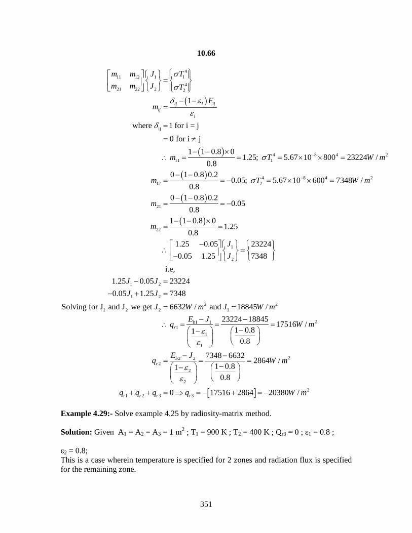
351
10.66
( )
( )
( )
4111 12 14
21 22 2 2
ij
4 8 4 211 1
4 8 412 2
1
where 1 for i = j
0 for i j1 1 0.8 0
1.25; 5.67 10 800 23224 /0.8
0 1 0.8 0.20.05; 5.67 10 600 7348 /
0.8
ij i ijij
i
Tm m Jm m J T
Fm
m T W m
m T W m
σ
σ
δ εε
δ
σ
σ
−
−
=
− −=
=
= ≠
− − ×∴ = = = × × =
− −= = − = × × =
( )
( )
2
21
22
1
2
1 2
1 22 2
1 2 2 1
1
0 1 0.8 0.20.05
0.81 1 0.8 0
1.250.8
1.25 0.05 232240.05 1.25 7348
i.e, 1.25 0.05 232240.05 1.25 7348
Solving for J and J we get 6632 / and 18845 /
r
m
m
JJ
J JJ J
J W m J W m
q
− −= = −
− − ×= =
− ∴ = −
− =− + =
= =
∴
[ ]
21 1
1
1
22 22
2
2
21 2 3 3
23224 18845 17516 /1 0.81
0.8
7348 6632 2864 /1 0.81
0.8
0 17516 2864 20380 /
b
br
r r r r
E J W m
E Jq W m
q q q q W m
εε
εε
− −= = =
− −
− −= = =
− −
+ + = ⇒ = − + = −
Example 4.29:- Solve example 4.25 by radiosity-matrix method. Solution: Given A1 = A2 = A3 = 1 m2 ; T1 = 900 K ; T2 = 400 K ; Qr3 = 0 ; ε1 = 0.8 ; ε2 = 0.8; This is a case wherein temperature is specified for 2 zones and radiation flux is specified for the remaining zone.

352
10.67 δij − (1 – εi) Fij
mij = ------------------------ for i = 1,2 and mij = δij − Fij for i = 3 εi 0 – (1 – 0.8) x 0.5 Therefore m11 = (1 – 0) / 0.8 = 1.25 ; m12 = ------------------------- = - 0.125 = m21
0.8 (1 – 0) 0 – (1 – 0.8) x 0.5 m22 = ------------ = 1.25 ; m13 = ------------------------ = − 0.125 = m23 0.8 0.8 m31= 0 – F31 = − 0.5 ; m32 = 0 – F32 = − 0.5 ; m33 = 1 – F33 = 1.0 The radiosity matrix equation can now be written as follows: σ T1
4
[mij]{Ji} = {S} where {S} = σ T24
0 In expanded form the above equation can be written as: m11 J1 + m12 J2 + m13 J3 = σ T1
4 m21 J1 + m22 J2 + m23 J3 = σ T2
4 m31 J1 + m32 J2 + m33 J3 = 0 Substituting the numerical values fo mij , T1, T2 and σ the above three equations can be solved for J1, J2 and J3.
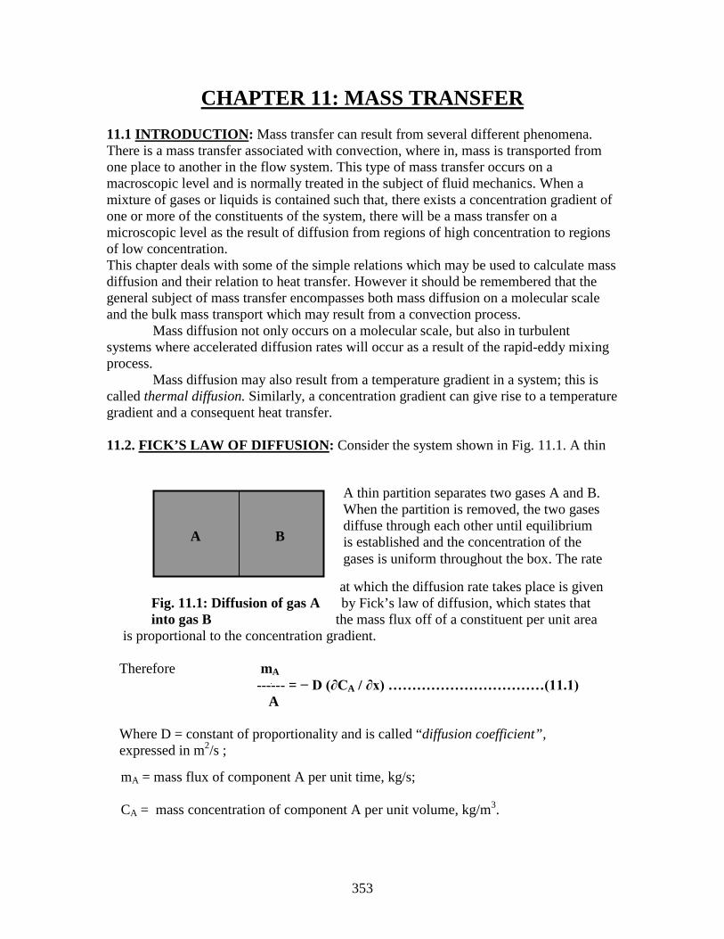
353
CHAPTER 11: MASS TRANSFER 11.1 INTRODUCTION: Mass transfer can result from several different phenomena. There is a mass transfer associated with convection, where in, mass is transported from one place to another in the flow system. This type of mass transfer occurs on a macroscopic level and is normally treated in the subject of fluid mechanics. When a mixture of gases or liquids is contained such that, there exists a concentration gradient of one or more of the constituents of the system, there will be a mass transfer on a microscopic level as the result of diffusion from regions of high concentration to regions of low concentration. This chapter deals with some of the simple relations which may be used to calculate mass diffusion and their relation to heat transfer. However it should be remembered that the general subject of mass transfer encompasses both mass diffusion on a molecular scale and the bulk mass transport which may result from a convection process. Mass diffusion not only occurs on a molecular scale, but also in turbulent systems where accelerated diffusion rates will occur as a result of the rapid-eddy mixing process. Mass diffusion may also result from a temperature gradient in a system; this is called thermal diffusion. Similarly, a concentration gradient can give rise to a temperature gradient and a consequent heat transfer. 11.2. FICK’S LAW OF DIFFUSION: Consider the system shown in Fig. 11.1. A thin
mA = mass flux of component A per unit time, kg/s; CA = mass concentration of component A per unit volume, kg/m3.
A B
A thin partition separates two gases A and B. When the partition is removed, the two gases diffuse through each other until equilibrium is established and the concentration of the gases is uniform throughout the box. The rate
at which the diffusion rate takes place is given Fig. 11.1: Diffusion of gas A by Fick’s law of diffusion, which states that into gas B the mass flux off of a constituent per unit area is proportional to the concentration gradient. Therefore mA
------ = − D (∂CA / ∂x) ……………………………(11.1) A Where D = constant of proportionality and is called “diffusion coefficient”, expressed in m2/s ;
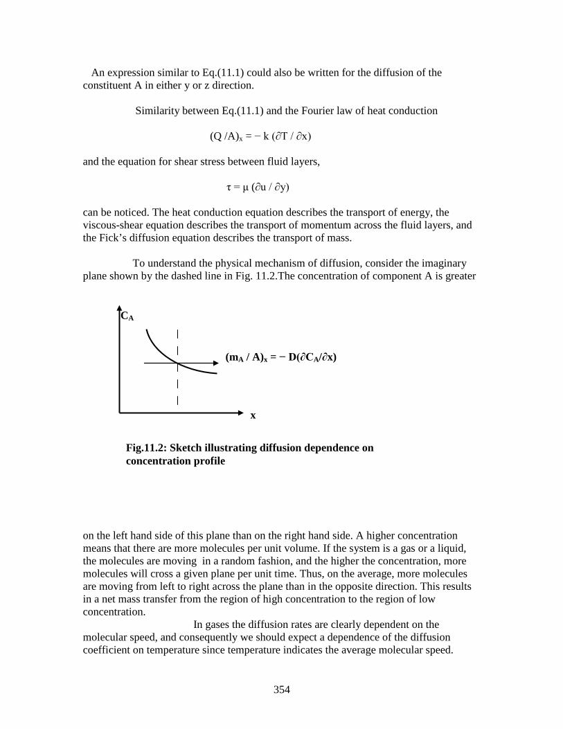
354
An expression similar to Eq.(11.1) could also be written for the diffusion of the constituent A in either y or z direction. Similarity between Eq.(11.1) and the Fourier law of heat conduction (Q /A)x = − k (∂T / ∂x) and the equation for shear stress between fluid layers, τ = μ (∂u / ∂y) can be noticed. The heat conduction equation describes the transport of energy, the viscous-shear equation describes the transport of momentum across the fluid layers, and the Fick’s diffusion equation describes the transport of mass. To understand the physical mechanism of diffusion, consider the imaginary plane shown by the dashed line in Fig. 11.2.The concentration of component A is greater
on the left hand side of this plane than on the right hand side. A higher concentration means that there are more molecules per unit volume. If the system is a gas or a liquid, the molecules are moving in a random fashion, and the higher the concentration, more molecules will cross a given plane per unit time. Thus, on the average, more molecules are moving from left to right across the plane than in the opposite direction. This results in a net mass transfer from the region of high concentration to the region of low concentration. In gases the diffusion rates are clearly dependent on the molecular speed, and consequently we should expect a dependence of the diffusion coefficient on temperature since temperature indicates the average molecular speed.
(mA / A)x = − D(∂CA/∂x)
x
CA
Fig.11.2: Sketch illustrating diffusion dependence on concentration profile

355
11.3. DIFFUSION IN GASES: GILLILAND has proposed a semi-empirical equation for the diffusion coefficient in gases: T 3 / 2 __________________ D = 435.7 ---------------------------- √[ (1 / MA) + (1 / MB) ] p [ VA
1/3 + VB1/3 ]
……………………….(11.2) In the above equation D is in cm 2/s, T is in degrees Kelvin, p is the total system pressure in pascals, and VA and VB are the molecular volumes of constituents A and B and MA and MB are the molecular weights of constituents A and B. Equation (11.2) offers a convenient expression for calculating the diffusion coefficients for various compounds and mixtures, but should not be used as a substitute for experimental values of the diffusion coefficients when they are available for a particular system. With reference to Fig.11.1, it can be stated that the diffusion process is occurring in two ways at the same time; that is gas A is diffusing into gas B and at the same time gas B is diffusing into gas A. We , therefore, could refer to the diffusion coefficient for either of these processes. While working with Eq. (11.1), one can use mass flux per unit area and mass concentrations, or the equation may be expressed in terms of molal concentrations and fluxes. There is no general rule to say which type of expression will be most convenient, and the specific problem under consideration will determine the one to be used. For gases Fick’s law may be expressed in terms of partial pressures by making use of the ideal-gas equation of state The ideal-gas equation of state can be written as p = ρRT ………………………………(11.3) The density ρ represents the mass concentration to be used in Fick’s law. The gas _ constant R for a particular gas may expressed in terms of the universal gas constant R and the molecular weight of the gas: _ R RA = ------- …………………………….(11.4) MA _ Where R = 8314 J/(kg-mol-K) _ or R = 0.08205 m3.atm/(kg-mol – K)

356
Consequently Fick’s law of diffusion for component A into component B can be written as follows: _ CA = ρA = (pAMA) / (R T) _ Hence ( ∂CA / ∂x) = [MA / (R T)] (dpA/dx) if isothermal diffusion is considered. Substituting this expression in Eq.(11.1) we have mA _
------ = − DAB [MA / (R T)] (dpA/dx) ………………..(11.5) A Similarly we can also write for the diffusion of component B into component A as mB _
------ = − DBA [MB / (R T)] (dpB/dx) ………………..(11.6) A Equation (11.6) also assumes isothermal diffusion process. Equimolal counter diffusion in gases:- Consider a physical situation as shown in Fig. 11.3: NA and NB represent the steady-state molal diffusion rates of components A and B,
respectively. In this steady-state situation each molecule of A is replaced by a molecule of B, and vice versa. The molal diffusion rates are given by
Δx 1 2
NA NB
Reservoir of B Reservoir of A
Fig. 11.3: Sketch illustrating equimolal diffusion

357
mA _
NA = ------ = − DAB [A / (R T)] (dpA/dx) MA mB _
NB = ------ = − DBA [A / (R T)] (dpB/dx) MB The total pressure of the system p remains constant at steady state, so that p = pA + pB = constant where pA and pB are partial pressures of gas A and gas B respectively. Therefore it follows that (dpA/dx) + (dpB/dx) = 0 or (dpA/dx) = − (dpB/dx) ………………………….(11.7) Since each molecule of A is replacing a molecule of B, the molal diffusion rates are equal:
− NA = NB Therefore DAB [A / (R T)] (dpA/dx) = − DBA [A / (R T)] (dpB/dx) Using Eq. (11.7), the above equation can be written as DAB = DBA = D …………………………………(11.8) Integration of Eq.(11.5) between section 1 and section 2 of Fig. 11.3 we get mA − DMA (pA2 – pA1) ----- = ---_---- ------------------ …………………..(11.9) A R T Δx Illustrative example 11.1:- Consider two large vessels, each containing uniform mixtures of nitrogen and carbon dioxide at 1 atm, and 288.9 K, but at different concentrations. Vessel 1 contains 90 mole percent N2 and 10 mole percent CO2, where as vessel 2 contains 20 mole percent N2 and 80 mole percent CO2. The two vessels are connected by a duct of 0.1524 m inside diameter and length of 1.22 m. Determine the rate of transfer of nitrogen between the two vessels by assuming that steady-state transfer takes place. The mass diffusivity for the N2 – CO2 mixture at 1 atm and 288.9 K is 0.16 x 10 − 4 m 2/s. Solution: In this mass transfer process, N2 is transferred from vessel 1 containing higher concentration of N2 to vessel 2 having lower concentration. In the early stages of mass transfer, the partial pressure of N2 in both vessels is considered to remain constant so that
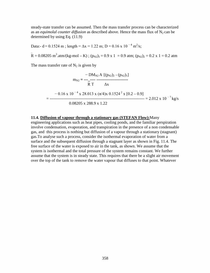
358
steady-state transfer can be assumed. Then the mass transfer process can be characterized as an equimolal counter diffusion as described above. Hence the mass flux of N2 can be determined by using Eq. (11.9) Data:- d = 0.1524 m ; length = Δx = 1.22 m; D = 0.16 x 10 − 4 m2/s; _ R = 0.08205 m3.atm/(kg-mol – K) ; (pN2)1 = 0.9 x 1 = 0.9 atm; (pN2)2 = 0.2 x 1 = 0.2 atm The mass transfer rate of N2 is given by − DMN2 A [(pN2)2 - (pN2)1] mN2 = ---_---- ----------------------- R T Δx − 0.16 x 10 − 4 x 28.013 x (π/4)x 0.1524 2 x [0.2 – 0.9] = --------------------------------------------------------------------- = 2.012 x 10 − 7 kg/s 0.08205 x 288.9 x 1.22 11.4. Diffusion of vapour through a stationary gas (STEFAN Flow):Many engineering applications such as heat pipes, cooling ponds, and the familiar perspiration involve condensation, evaporation, and transpiration in the presence of a non condensable gas, and this process is nothing but diffusion of a vapour through a stationary (stagnant) gas.To analyse such a process, consider the isothermal evaporation of water from a surface and the subsequent diffusion through a stagnant layer as shown in Fig. 11.4. The free surface of the water is exposed to air in the tank, as shown. We assume that the system is isothermal and the total pressure of the system remains constant. We further assume that the system is in steady state. This requires that there be a slight air movement over the top of the tank to remove the water vapour that diffuses to that point. Whatever

359
air movement may be necessary to accomplish this, it is assumed that it does alter the concentration profiles in the air in the tank.We further assume that air and water vapour behave as ideal gases. As the water evaporates, it will diffuse upward through the air, and at steady state this upward movement must be balanced by a downward diffusion of air so that the concentration at any x will remain constant. But at the surface of the water there can be no net mass movement of air downward. Consequently there must be a bulk mass movement upward with a velocity just large enough to balance the diffusion of air downward. This bulk mass movement then produces an additional mass flux of water vapour upward. The diffusion of air downward is given by (see Eq. 11.5) _
mA = − DAB A [MA / (R T)] (dpA/dx) ………………..(11.10) where A denotes the cross sectional area of the tank. This must be balanced by the bulk-mass transfer upward. If u is the bulk-mass velocity then pAMA mA = − ρAAu = − -------- Au R T DAW or u = -------- (dPA/dx) ……………………….(11.11) pA Mass diffusion of water vapour is given by
Water 1
2 Air
x
p
pw pA
Fig. 11.4: Diffusion of water vapour into air
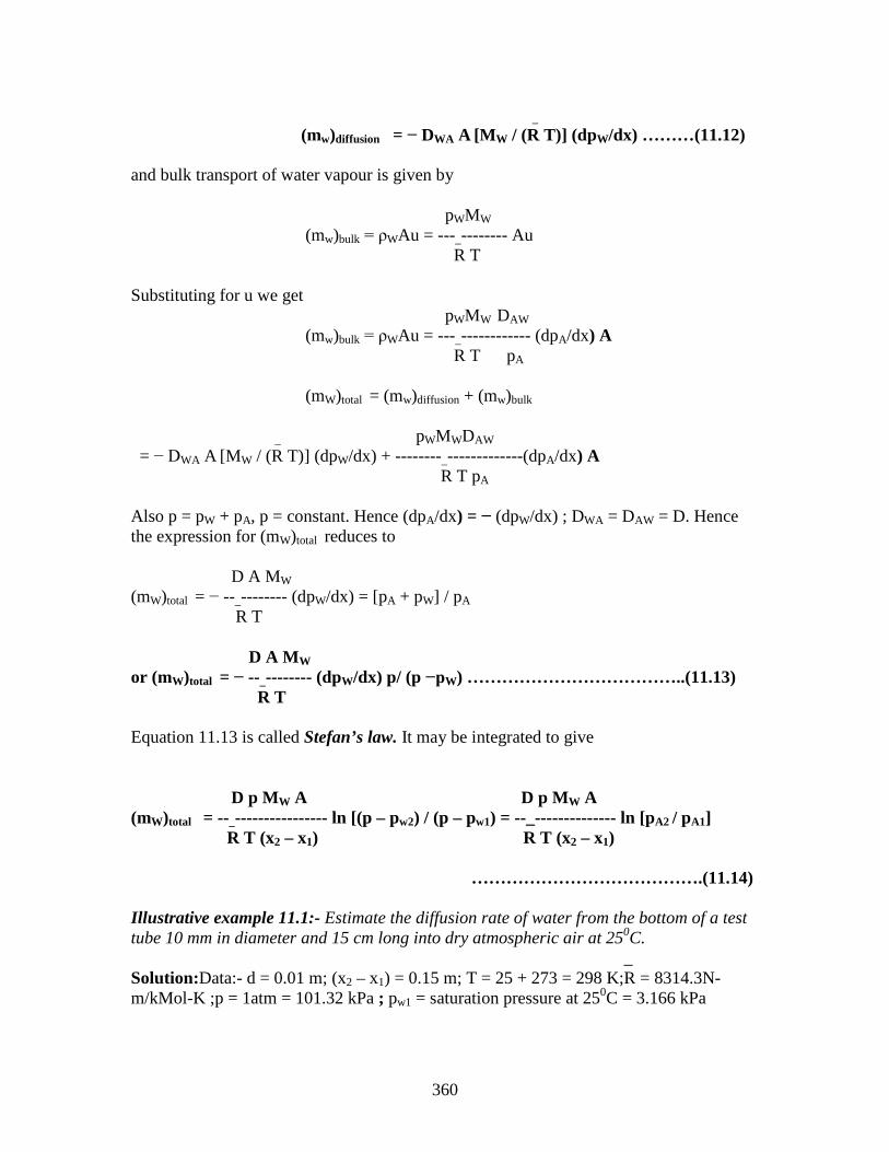
360
_ (mw)diffusion = − DWA A [MW / (R T)] (dpW/dx) ………(11.12) and bulk transport of water vapour is given by pWMW (mw)bulk = ρWAu = ---_-------- Au R T Substituting for u we get pWMW DAW (mw)bulk = ρWAu = ---_------------ (dpA/dx) A R T pA (mW)total = (mw)diffusion + (mw)bulk _ pWMWDAW = − DWA A [MW / (R T)] (dpW/dx) + --------_-------------(dpA/dx) A R T pA Also p = pW + pA, p = constant. Hence (dpA/dx) = − (dpW/dx) ; DWA = DAW = D. Hence the expression for (mW)total reduces to D A MW (mW)total = − --_-------- (dpW/dx) = [pA + pW] / pA R T D A MW or (mW)total = − --_-------- (dpW/dx) p/ (p −pW) ………………………………..(11.13) R T Equation 11.13 is called Stefan’s law. It may be integrated to give D p MW A D p MW A (mW)total = --_---------------- ln [(p – pw2) / (p – pw1) = --_-------------- ln [pA2 / pA1] R T (x2 – x1) R T (x2 – x1) ………………………………….(11.14) Illustrative example 11.1:- Estimate the diffusion rate of water from the bottom of a test tube 10 mm in diameter and 15 cm long into dry atmospheric air at 250C. _ Solution:Data:- d = 0.01 m; (x2 – x1) = 0.15 m; T = 25 + 273 = 298 K;R = 8314.3N-m/kMol-K ;p = 1atm = 101.32 kPa ; pw1 = saturation pressure at 250C = 3.166 kPa

361
From tables for diffusion of water into air D = 0.256 cm 2/s; We use Eq.(11.14) to calculate the mass flux. The partial pressure of water vapour at the bottom of the test tube is the saturation temperature of water at 250C and at the top the partial pressure of water vapour is zero as the air is dry (i.e. pw2 = 0). Substituting the values in Eq.(11.14) we have (0.256 x 10 − 4) x 18 x (π x 0.005 2) (mw)total = ------------------------------------------- ln [(101.32 – 0) / (101.32 – 3.166)] 8314.3 x298 x 0.15 = 3.131 x 10 − 10 kg/s 11.5. Steady State Diffusion in Liquids: Steady state Equimolal Counter Diffusion in Liquids:- The analysis for steady state counter diffusion in liquids follows the same approach as that for gases. In terms of number of mole flux of species A ,Fick’s law can be written as NA = (mA / MA) = − D (∂CA / ∂x) ……………………..(11.15) The integration of Eq.(11.15) from x = x1 to x = x2 with CA varying from CA1 to CA2,gives (CA1 − CA2 ) NA = D ---------------- ………………………………….(11.16) (x2 – x1) The above equation can also be expressed in terms of mole fractions of species at locations x1 and x2 as follows. Mole fraction at x1 = (CA1 / C ) = χA1; Mole fraction at x2 = χA2 = CA2 /C. Where C = Total molal concentration of the mixture. Eq.(11.16) can be written in terms of mole fraction as (χA1 − χA2) NA = DC -------------- kg-mol /(m2-s) …………………(11.17) (x2 – x1) Steady State Unidirectional Diffusion in liquids:- The analysis for the determination of the concentration distribution during steady state unidirectional diffusion in liquids is exactly same as that for gases except that in the case of liquids the equation is derived in terms of molal concentrations CA and CB instead of partial pressures.

362
If NA = molal flux of species A per unit area, then C ( CB2 – CB1) C ( CA1 – CA2) NA = D ---------------- ------------------ = D ----------------- ------------------ ……(11.18 a) ( x2 – x1 ) CB ln ( x2 – x1 ) CB ln Where the logarithmic mean concentration CB ln of component B is defined as ( CB2 – CB1) CB ln = -------------------- ……………………..(11.18 b) ln (CB2 / CB1) Also C = CA + CB and CB2 – CB1 = ( CA1 – CA2). Equations (11.18) can also be written in terms ox mole fractions: C ( χB2 – χB1) C ( χA1 – χA2) NA = D ---------------- ------------------ = D ----------------- ------------------ ……(11.19 a) ( x2 – x1 ) χB ln ( x2 – x1 ) χB ln Where the logarithmic mean mole fraction χB ln of component B is defined as ( χB2 – χB1) χB ln = -------------------- ……………………..(11.19 b) ln (χB2 / χB1) In Eqs.(11.18) and (11.19), the units of various quantities may be taken as Ci = molal concentration, i = A, or B, kg-mol/m3 χi = Ci / C = mole fraction of component i C = molal concentration of the mixture, kg-mol/m3 D = mass diffusivity, m2/s NA = molal flux of species A, kg-mol /(m2-s) X = distance,m
11.6. Solution to tutorial problems: 11.1 Solution: Data:- p = 1 atm; T = 273 K; (CA)1 = 0.8; (Cso2)1 = 0.20; (CA)2 = 0.30; (Cso2)1 = 0.70; d = 0.1 m ; Δx = 1.8 m
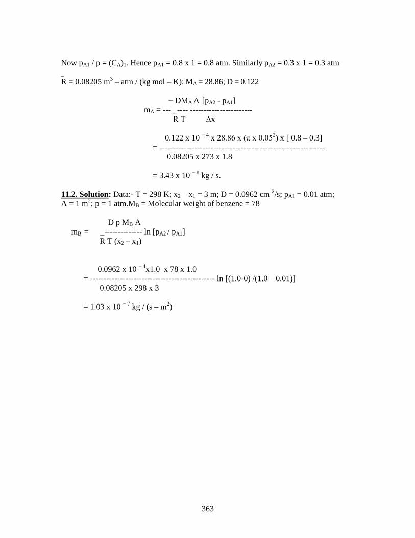
363
Now pA1 / p = (CA)1. Hence pA1 = 0.8 x 1 = 0.8 atm. Similarly pA2 = 0.3 x 1 = 0.3 atm _ R = 0.08205 m3 – atm / (kg mol – K); MA = 28.86; D = 0.122 − DMA A [pA2 - pA1] mA = --- _---- ----------------------- R T Δx 0.122 x 10 − 4 x 28.86 x (π x 0.052) x [ 0.8 – 0.3] = ------------------------------------------------------------- 0.08205 x 273 x 1.8 = 3.43 x 10 − 8 kg / s. 11.2. Solution: Data:- T = 298 K; x2 – x1 = 3 m; D = 0.0962 cm 2/s; pA1 = 0.01 atm; A = 1 m2; p = 1 atm.MB = Molecular weight of benzene = 78 D p MB A mB = _-------------- ln [pA2 / pA1] R T (x2 – x1) 0.0962 x 10 − 4x1.0 x 78 x 1.0 = ---------------------------------------------- ln [(1.0-0) /(1.0 – 0.01)] 0.08205 x 298 x 3 = 1.03 x 10 − 7 kg / (s – m2)

364


