HEAT TRANSFER SIMULATION FROM FINS OF AN AIR-COOLED ENGINE … · engine. This force moves the...

HEAT TRANSFER SIMULATION FROM

FINS OF AN AIR-COOLED ENGINE BY USING CFD

A PROJECT REPORT

Submitted by

ARAVIND.B 12008114006

DASAN SISIL RAJ.G 12008114021

DINESH.R 12008114024

SURESH KUMAR.K 12008114101

In partial fulfilment for the award of the degree

Of

BACHELOR OF ENGINEERING

IN

MECHANICAL ENGINEERING

VELAMMAL ENGINEERING COLLEGE, CHENNAI

ANNA UNIVERSITY: CHENNAI – 600 025

APRIL 2012

ANNA UNIVERSITY: CHENNAI 600 025

BONAFIDE CERTIFICATE

Certified that this project report “Heat Transfer Simulation from Fins of an

Air-cooled Engine by Using CFD” is the bonafide work of “Aravind.B,

Dinesh.R, Dasan Sisil Raj.G, Suresh Kumar.K” who carried out the project

work under my supervision.

SIGNATURE SIGNATURE

Dr. M. Balasubramanian Mr. M. Karthick

HEAD OF THE DEPARTMENT SUPERVISOR

Department of Mechanical Engineering Assistant Professor

Velammal Engineering College Department of Mechanical Engineering

Velammal Engineering College

CERTIFICATE OF EVALUATION

College Code and Name : 120, Velammal Engineering College, Chennai.

Branch & Semester : Mechanical Engineering / VIII Semester.

S.

NO

NAME OF THE

STUDENTS

REG

NUMBER TITLE OF PROJECT

1 ARAVIND.B

12008114006 HEAT TRANSFER

SIMULATION BY

CFD FROM FINS OF

AN AIR-COOLED

ENGINE

2 DASAN SISIL RAJ.G

12008114021

3 DINESH.R

12008114024

4 SURESH KUMAR.K 12008114101

The report of the project work submitted by the above students in partial

fulfilment for the award of Bachelor of Engineering Degree in MECHANICAL

ENGINEERING of Anna University, Chennai was evaluated and confirmed to

be the report of work done by above students and then evaluated

INTERNAL EXAMINER EXTERNAL EXAMINER

ACKNOWLEDGEMENT

We express our sincere thanks to Shri. M.V. Muthuramalingam, Chairman,

Mr. M.V.M. Velmurugan, CEO, Dr.R.S. Kumar, Principal and

Dr.G.Prabhakaran, Vice-Principal of Velammal Engineering College for

their support and creating a comfortable atmosphere required for this project.

We are very much grateful to Dr.M. Balasubramanian, Professor and Head

of Department of Mechanical Engineering, Velammal Engineering College

for his encouraging support and useful suggestions during this work.

We express our profound sense of gratitude to Mr. M. Karthick, Assistant

Professor, Department of Mechanical Engineering, Velammal Engineering

College for his excellent guidance, help and constant encouragement throughout

the project work as our project guide.

We take this opportunity to thank all teaching members of our department for

their suggestion and help. We also thank all non-teaching staff for their co-

operation and help during this project work.

Last but not the least; we thank our parents who have been the source of

inspiration and support for us throughout this project work. We also thank all

those who have either directly or indirectly helped during this project work.

ABSTRACT

The main objective of this project is to analyze the various

cross-sections of fins which are currently being used in air cooled engines

for heat transfer by using CFD.Initially various details about the current

trends in engine designing were studied. The various dimensions of all the

components of the engine are measured using standard measurement tools

such as Vernier callipers, metre scale, etc. Various preliminary designs were

obtained which were then subjected to different analysis and finally a

modified design will thus be arrived.

The various parameters taken into consideration for optimization are

✓ Heat transfer rate

✓ Air Flow & Resistance Offered To Flow

✓ Surface Area

✓ Weight of the component

✓ Cost

The proposed design of the fin is considered to be far more effective and

efficient than the existing design. It also involves least amount of material

among all different alternatives and hence it requires less cost for production.

This project aims to achieve an optimized design for engine fins.

CONTENTS

Chapter no. Title Page no.

List of Figures

List of Tables

List of Symbols & Notations

i

ii

iii

1. Introduction

1.1 About IC Engines

1.2 Brief History of IC Engines

1.3 Types of IC Engines

1.4 Working of IC Engines

1.5 IC Engine – Cooling System

1.6 Heat Transfer

1.7 Heat Transfer through Fins

1.8 Fin Cross-Sections

1.9 Fin Materials

1.10 Fin Uses

1

1

2

2

3

4

6

8

10

11

11

2. Literature review 12

3. Single-Cylinder Four Stoke SI Engine

3.1 Engine Specifications

3.2 Cylinders

3.3 Pistons

3.4 Crankshaft & Connecting Rod

3.5 Flywheel

3.6 Heat Sink

16

16

17

18

18

18

4. Software’s Used

4.1 Introduction to Pro/E Wildfire 5.0

4.2 ANSYS CFX

19

21

5. Design of Fins

5.1 Rectangular Fin

5.2 Parabolic Fin

26

28

6. Modeling & Analysis

6.1 Pro/ENGINEER Modeling

6.1.1 Rectangular Fin

6.1.2 Trapezoidal Fin

6.1.3 Parabolic-1 Fin


33

34

36

37

6.2 Analysis in ANSYS





6.3 Bajaj Pulsar 150cc Engines

39

45

51

57

63

7. Results & Discussions

7.1 Comparison of Various Fin Parameters

7.2 Results

References

71

72

73

List of Figures

Fig no. Description Page no.

1.1 Stages of IC Engine Combustion 3

1.2 Triangular, Rectangular & Trapezoidal Fins 10

1.3 Parabolic & Cylindrical Fins 10

3.1

4.1

4.2

Single Cylinder 4-Stroke Engine

Spray Development in IC Engines

BorgWarner Turbo & Emission Systems

17

23

24

5.1 Rectangular Fin 26

5.2 Parabolic Fin (Case 1) 28

5.3 Parabolic Fin Efficiency 29

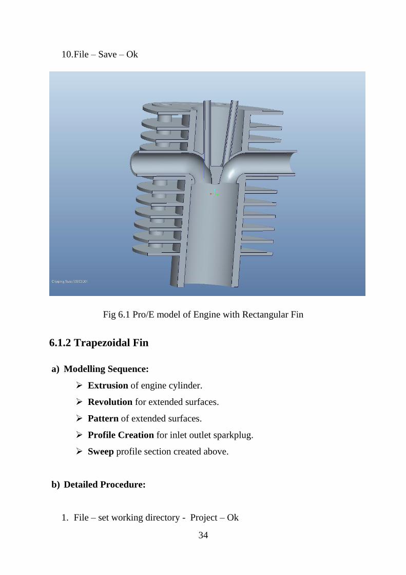
6.1 Pro/E model of Engine w/ Rectangular Fin 34

6.2 Pro/E model of Engine w/ Trapezoidal Fin 35

6.3

6.4

Pro/E model of Engine w/ Parabolic-1 Fin

Pro/E model of Engine w/ Parabolic-2 Fin

37

38

6.5

6.6

6.7

6.8

6.9

6.10

6.11

6.12

6.13

6.14

6.15

6.16

Meshed View (Rectangular Fin)

Temperature Contour (Rectangular Fin)

Heat Flux Contour (Rectangular Fin)

Stream Flow (Rectangular Fin)

Temperature Bar chart (Rectangular Fin)

Heat Flux Bar Chart (Rectangular Fin)

Temperature Vs Length (Rectangular Fin)

Velocity Vs Length (Rectangular Fin)

h Vs Length (Rectangular Fin)

Meshed View (Trapezoidal Fin)

Temperature Contour (Trapezoidal Fin)

Heat Flux Contour (Trapezoidal Fin)

40

41

41

42

42

43

43

44

44

46

47

47

6.17

6.18

6.19

6.20

6.21

6.22

6.23

6.24

6.25

6.26

6.27

6.28

6.29

6.30

6.31

6.32

6.33

6.34

6.35

6.36

6.37

6.38

6.39

6.40

6.41

6.42

6.43

6.44

Stream Flow (Trapezoidal Fin)

Temperature Bar chart (Trapezoidal Fin)

Heat Flux Bar Chart (Trapezoidal Fin)

Temperature Vs Length (Trapezoidal Fin)

Velocity Vs Length (Trapezoidal Fin)

h Vs Length (Trapezoidal Fin)

Meshed View (Parabolic-1 Fin)

Temperature Contour (Parabolic-1 Fin)

Heat Flux Contour (Parabolic-1 Fin)

Stream Flow (Parabolic-1 Fin)

Temperature Bar chart (Parabolic-1 Fin)

Heat Flux Bar Chart (Parabolic-1 Fin)

Temperature Vs Length (Parabolic-1 Fin)

Velocity Vs Length (Parabolic-1 Fin)

h Vs Length (Parabolic-1 Fin)

Meshed View (Parabolic-2 Fin)

Temperature Contour (Parabolic-2 Fin)

Heat Flux Contour (Parabolic-2 Fin)

Stream Flow (Parabolic-2 Fin)

Temperature Bar chart (Parabolic-2 Fin)

Heat Flux Bar Chart (Parabolic-2 Fin)

Temperature Vs Length (Parabolic-2 Fin)

Velocity Vs Length (Parabolic-2 Fin)

h Vs Length (Parabolic-2 Fin)

Pulsar Engine (Original)

Temperature Contour (Original)

Temperature Contour (Case 1)

Temperature Contour (Case 2)

48

48

49

49

50

50

52

53

53

54

54

55

55

56

56

58

59

59

60

60

61

61

62

62

63

63

64

64

6.45

6.46

6.47

6.48

6.49

6.50

6.51

6.52

6.53

6.54

6.55

6.56

Heat Flux Contour (Original)

Heat Flux Contour (Case 1)

Heat Flux Contour (Case 2)

Stream flow (Original)

Stream flow (Case 1)

Stream flow (Case 2)

Temperature vs. Length (Original)

Temperature vs. Length (Case 1)

Temperature vs. Length (Case 2)

Velocity vs. Length (Original)

Velocity vs. Length (Case 1)

Velocity vs. Length (Case 2)

65

65

66

66

67

67

68

68

69

69

70

70

i

List of Tables

Table

no.

Description Page no.

1

2

Mesh Information (Rectangular Fin)

Mesh Information (Trapezoidal Fin)

40

46

3 Mesh Information (Parabolic-1 Fin) 52

4 Mesh Information (Parabolic-2 Fin) 58

5

Comparison of various Profiles

71

ii

List of Symbols & Notations

Term Symbol/Notation

Efficiency η

Convective heat transfer coefficient

Fin Effectiveness

Fin Efficiency

Overall Surface Efficiency

Thermal Conductivity

Heat transfer along the length of Fin

Heat transfer at the base of Fin

Heat transfer without Fin

Fin Base Temperature

Surrounding Temperature

Bare Surface Area

Surface area of fin

Surface area of engine without fin

h

𝜖𝑓

𝜂𝑓

𝜂𝑜

K

𝑄𝑙

𝑄𝑏

𝑄𝑤𝑓

𝑇𝑏

𝑇∞

𝐴𝑏

𝐴𝑠

𝐴𝑤𝑓

iii

1

CHAPTER 1

1. Introduction

A fin is a surface that extends from an object to increase the rate of

heat transfer to or from the environment by increasing convection. Increasing

the temperature difference between the object and the environment, increasing

the convection heat transfer coefficient, or increasing the surface area of the

object increases the heat transfer. Sometimes it is not economical or it is not

feasible to change the first two options. Adding a fin to an object, however,

increases the surface area and can sometimes be an economical solution to heat

transfer problems. The Selection of a proper fin is very essential in establishing

the heat transfer as the fin’s shape and dimensions affect the heat transfer to

great extent. Our project deals with the design and analysis of various fin cross-

sections by CFD to determine the heat transfer for each fin and to find out the

effective cross-section.

1.1 About IC Engines

The internal combustion engine is an engine in which the

combustion of a fuel occurs with air inside a combustion chamber. In an internal

combustion engine, the expansion of the high-temperature and high –pressure

gases produced by combustion apply direct force to some component of the

engine. This force moves the component over a distance, transforming chemical

energy into useful mechanical energy.

The internal combustion engine can work in two, four and even in

six strokes. Commonly two-stroke IC engine are used in motor cycles and four-

stroke IC engine are used in automobiles, trucks etc.

2

The IC engines use fossil fuels like petrol (gasoline), diesel and some gaseous

fuels and a mixture of liquid-gas fuel.

1.2 Brief History of IC Engines

Christiaan Huygens designs gunpowder to drive water pumps, to

supply 3000 cubic meters of water/day for the Versailles palace gardens,

essentially creating the first idea of a rudimentary internal combustion piston

engine in 17th century. The engine was based on the Stirling cycle which is a

closed cycle regenerative cycle. Hence all engines having working principle

based on the Stirling cycle were named Stirling engines. In 1823, Samuel

Brown patented the first internal combustion engine to be applied industrially.

It was compression less and based on what Hardenberg calls the “Leonardo

cycle,” which, as the name implies, was already out of date at that time. Later in

1862, German inventor Nikolaus Otto was the first to build and sell the engine.

He designed an indirect-acting free-piston compression less engine whose

greater efficiency won the support of Eugen Langen and then most of the

market, which at that time was mostly for small stationary engines fuelled by

lighting gas. Rudolf Diesel demonstrated the diesel engine in the 1900 using

peanut oil (biodiesel)

1.3 Types of IC Engines

There are generally 2 main types of Stirling engines.

a) Reciprocating IC Engine

A Reciprocating IC engine consists of a piston in a cylinder which

is free to slide inside the cylinder along the stroke length. The piston has piston

rings which are in contact with cylinder walls.

3

The reciprocating output of the piston is converted to the rotational motion

using connecting rod and crank shaft. The rotational power generated is utilized

for useful purposes.

b) Rotary IC Engine

Wankel engine is a rotary IC engine. The Wankel engine (rotary

engine) does not have piston strokes. It operates with the same separation of

phases as the four-stroke engine with the phases taking place in separate

locations in the engine. In thermodynamic terms it follows the Otto engine

cycle, so may be thought of as a “four-phase” engine. While it is true that three

power strokes typically occur per rotor revolution due to the 3:1 revolution ratio

of the rotor to the eccentric shaft, only one power stroke per shaft revolution

actually occurs; this engine provides three power ‘strokes’ per revolution per

rotor giving it a greater power-to-weight ratio than piston engines.

1.4 Working of IC Engines

Fig 1.1 Stages of IC engine Combustion

4

Internal combustion engines have four basic steps that repeat with every two

revolutions for four-stroke and one revolution for two-stroke engine:

1. Intake stroke: The first stroke of the internal combustion engine is also

known as the suction stroke because the piston moves to the maximum volume

position (downward direction in the cylinder). The inlet valve opens as a result

of piston movement, and the vaporized fuel mixture enters the combustion

chamber. The inlet valve closes at the end of this stroke.

2. Compression stroke: In this stroke, both valves are closed and the piston

starts its movement to the minimum volume position (upward direction in the

cylinder) and compresses the fuel mixture. During the compression process,

pressure, temperature and the density of the fuel mixture increases.

3. Power stroke: When the piston reaches the minimum volume position, the

spark plug ignites the fuel mixture and burns. The fuel produces power that is

transmitted to the crank shaft mechanism.

4. Exhaust stroke: In the end of the power stroke, the exhaust valve opens.

During this stroke, the piston starts its movement in the minimum volume

position. The open exhaust valve allows the exhaust gases to escape the

cylinder. At the end of this stroke, the exhaust valve closes, the inlet valve

opens, and the sequence repeats in the next cycle. Four-stroke engines require

two revolutions.

Many engines overlap these steps in time: Jet engines do all steps

simultaneously at different parts of the engines.

1.5 IC Engine – Cooling System

In the Combustion Chamber, the fuel along with air is burned to

produce thermal energy.

5

This thermal energy is converted into mechanical energy by the piston &

cylinder setup and utilized to run the vehicle. Not all the thermal energy that is

produced is converted to useful work. Some energy is absorbed by the piston &

cylinder which raises the heat of the engine. The heating of engine parts is not

desired as it will damage the engine parts and burn the lubricants. So, cooling

must be done.

Engines with higher efficiency have more energy leave as

mechanical motion and less as waste heat. Some waste heat is essential: it

guides heat through the engine, much as a water wheel works only if there is

some exit velocity (energy) in the waste water to carry it away and make room

for more water. Thus, all heat engines need cooling to operate. Cooling is also

needed because high temperatures damage engine materials and lubricants.

Internal-combustion engines burn fuel hotter than the melting temperature of

engine materials, and hot enough to set fire to lubricants. Engine cooling

removes energy fast enough to keep temperatures low so the engine can survive.

Air-cooled and liquid-cooled engines are both used commonly.

Each principle has advantages and disadvantages, and particular applications

may favour one over the other. For example, most cars and trucks use liquid-

cooled engines, while many small airplane and low-cost engines are air-cooled.

a) Air-Cooled Engine

Cars and trucks using direct air cooling uses atmospheric air to

remove the heat from the engine. Fins are used for increasing the area of

exposure of the engine to the flowing air. The air at very high velocity flows

over the surface of the fins and collects the heat and it gets exhausted back into

the atmosphere. This uses both the conduction and forced convection mode of

heat transfer.

6

Advantage: “AIR” is naturally available in atmosphere. So, the coolant is

cheap and abundant. It also eliminates the need for some complex circuits

to handle the coolant. Thus making the engine more compact in size and

light in weight.

Disadvantage: The machining of fin follows number of processes and it is

considered to be tedious process. The heat transfer rate is not stable and

changes with temperature and pressure.

b) Liquid-Cooled Engine

Liquid-Cooling is mostly employed in marine vehicles which uses sea

water to remove the heat from engine. In some cases, chemical coolants are also

employed (in closed systems) or they are mixed with seawater cooling.

Advantage: Heat transfer from the engine to the sea water is high.

Disadvantage: Because of the high temperature and pressure of sea water

acquired by collecting the heat from the engine cylinder, the sea water

becomes an agent to cause severe corrosion in the coolant pipes. When the

atmospheric temperature is very low, it freezes the coolant and it stuck in

the pipelines. Thus causing a trouble to start the engine.

1.6 Heat Transfer

Heat transfer is concerned with the generation, use, conversion

and exchange of thermal energy and heat between physical systems. The heat

exchanging aspect found its application in most of the cooling systems in

automobile and various manufacturing machines used in workshops. So, the

exchange of heat between the system and surrounding must be effective in order

to reduce the power input and increases the power output.

7

The Heat transfer can takes place through all the phases of matter

i.e. Solids, liquids, gases and even through vacuum. Depending on the mode of

heat transfer, it is classified as:

➢ Conduction

➢ Convection

➢ Radiation

The convection mode of heat transfer found its application in most

of the automobile parts and in almost all the industries in the present world.

Convection is defined as transfer of heat from one place to

another through the bulk motion of the fluids. The fluid collects the heat from a

solid or another fluid through diffusion and transfers it to other substrate.

Among the three mode of heat transfer, the behaviour of the

convective heat transfer is complicated and the rate of heat transfer is not

constant. The rate of heat transfer is influenced by a number of parameters

which change with time. So, the design of the convective system must be

optimized to improve the efficiency and effectiveness of the system.

Mathematically the convective heat transfer is represented by

Newton’s law of Cooling: which states that “The rate of heat loss of a body is

proportional to difference in temperatures between the body and its

surroundings”. It is given by

𝑑𝑄

𝑑𝑡 = �̇� = ℎ. 𝐴. (𝑇𝑒𝑛𝑣 − 𝑇(𝑡)) = −ℎ. 𝐴∆𝑇(𝑡)

Where,

Q is thermal energy in joules

h is heat transfer co-efficient

8

A is surface area of heat being transferred

T is temperature of objects surface and interior

Tenv is the temperature of environment

ΔT(t) is the time-dependent thermal gradient between

environment and object.

One possible approach for development is to vary the surface area

and the heat transfer co-efficient to improve the rate of heat transfer.

1.7 Heat Transfer through Fins

The Rate of heat transfer in the fin is affected by number of fixed

and variable parameters which makes it more complex to determine the

performance of the fin. The performance varies independently. The heat transfer

from a fin is influenced by many fixed and variable parameters such as air flow

velocity, temperature, heat flux at cylinder wall, fin geometry, size, shape,

material etc.

Fin performance can be described in three different ways. To

optimize the fin performance, modifications are done to improve all the

following factors.

Fin Effectiveness: It is the ratio of the fin heat transfer rate to

the heat transfer rate of the object if it had no fin. It is denoted by εf.

𝜖𝑓 = 𝑞𝑓

ℎ. 𝐴𝑐,𝑏 . 𝜃𝑏

Where Ac.b is the fin cross-sectional area at the base.

9

Fin Efficiency: It is the ratio of the fin heat transfer rate to the

heat transfer rate of the fin if the entire fin were at the base temperature. It is

denoted by ηf.

𝜂𝑓 = 𝑞𝑓

ℎ. 𝐴𝑓 . 𝜃𝑏

Af in this equation is equal to the surface area of the fin. Fin

efficiency will always be less than one.

This is because assuming the temperature throughout the fin is at

the base temperature would increase the heat transfer rate.

Overall Surface Efficiency: It is the efficiency for an array of

fins. It is denoted by ηo.

𝜂𝑜 = 𝑞𝑡

ℎ. 𝐴𝑡 . 𝜃𝑏

Where At is the total area and qt is the sum of the heat transfer

rates of all the fins.

The fin performance and the heat transfer rate can be increased

in two different ways:

➢ To increase convection heat transfer coefficient h.

➢ To increase the surface area As.

Increasing h may require the installation of a pump or fan, or

replacing the existing pumps or fans with a larger ones. This approach in some

cases may or may not be practical. Besides in some cases, it may not be

adequate. The alternative is to increase the surface area by modifying the cross-

section of the fin.

10

1.8 Fin Cross-Sections

According to the Newton’s law of cooling,

Q=-h.A.ΔT

the rate of heat transfer is proportional to the surface area. So as the surface area

increases, the heat transfer and hence the fin performance increases. The cross-

section must be chosen in such a way that the surface area is more in order to

improve the area of contact with the fluid.

Some commonly used fins based on their cross-section is shown

below:

11

1.9 Fin Materials

Another way to increase the heat transfer is by selecting a proper

material which has a high thermal conductivity and less weight.

Aluminium is commonly used in making fin because of its

lighter weight. Aluminium is remarkable for the metal’s low density and for its

ability to resist corrosion due to the phenomenon of passivation.

Structural components made from aluminium and its alloys are

vital to the aerospace industry and are important in other areas of transportation

and structural materials. The most useful compounds of aluminium, at least on a

weight basis, are the oxides and sulphates. The thermal conductivity of

aluminium is 237 W·m−1·K−1

Other materials such as Copper ( 401 W·m−1·K−1 ), Steel etc. can

also be used.

1.10 Fin Uses

Fins are most commonly used in heat exchanging devices such

as radiators in cars and heat exchangers in power plants. They are also used in

newer technology such as hydrogen fuel cells. Nature has also taken advantage

of the phenomena of fins. The ears of jackrabbits and Fennec Foxes act as fins

to release heat from the blood that flows through them.

12

CHAPTER 2

2. Literature Review

Pulkit Agarwal, Mayur Shrikhande and P. Srinivasan [4].An air-cooled

motorcycle engine releases heat to the atmosphere through the mode of forced

convection. To facilitate this, fins are provided on the outer surface of the

cylinder. The heat transfer rate depends upon the velocity of the vehicle, fin

geometry and the ambient temperature. Many experimental methods are

available in literature to analyze the effect of these factors on the heat transfer

rate. However, an attempt is made to simulate the heat transfer using CFD

analysis. The heat transfer surface of the engine is modeled in GAMBIT and

simulated in FLUENT software. An expression of average fin surface heat

transfer coefficient in terms of wind velocity is obtained. It is observed that

when the ambient temperature reduces to a very low value, it results in

overcooling and poor efficiency of the engine.

Dhritiman Subha Kashyap [2].In the quest for designing better, more powerful

and fuel efficient engines, engine thermal management system design plays a

pivotal part. Optimal engine operating efficiency demands optimal heat transfer,

which, in turn, demands on accurate determination of the heat transfer co-

efficient. This parameter depends on a variety of factors like air flow speed over

the fins, operating temperature, fin width and pitch. Factors like air flow and

operating temperature change frequently, so predicting an all-encompassing

formula for predicting the heat transfer co-efficient is highly non-trivial in

nature. This paper looks at some efforts, both experimental and computer

simulations, to formulate this. Moreover, it also tries to evaluate the

assumptions used for deriving the formulas, in an effort to find the

shortcomings plaguing each of these in some aspect.

13

Rosli Abu Bakar, Chiew Chen Wee, Gan Leong Ming [6].The extended

surfaces for the cooling purpose were removable where it is attached onto the

engine block using fasteners. Two types of analyses were carried out, which are

the thermal analysis and the static analysis using the results from the thermal

analysis. The results showed that the removable fins are transferring heats like

normal fins but have higher temperature and the deformations are rather small.

The high temperature causes high thermal stresses on the cylinder assembly.

S.H. Barhatte, M. R. Chopade, V. N. Kapatkar [5].Extended surfaces,

commonly known as fins, often offer an economical and trouble free solution in

many situations demanding natural convection heat transfer. Heat sinks in the

form of fin arrays on horizontal and vertical surfaces used in variety of

engineering applications, studies of heat transfer and fluid flow associated with

such arrays are of considerable engineering significance. The main controlling

variable generally available to designer is geometry of fin arrays. Considering

the above fact, natural convection heat transfer from vertical rectangular fin

arrays with and without notch at the center have been investigated

experimentally and theoretically. Moreover notches of different geometrical

shapes have also been analyzed for the purpose of comparison and optimization.

In the present study, the fin flats are modified by removing the central fin

portion by cutting a notch. This paper presents an experimental analysis of the

results obtained over a range of, fin heights and heat dissipation rate. Attempts

are made to establish a comparison between the experimental results and results

obtained by using CFD software.

S. V. Naidu, V. Dharma Rao, B. Govinda Rao, A. Sombabu and B.

Sreenivasulu [1].The problem of natural convection heat transfer from fin arrays

with inclination is studied experimentally and theoretically to find the effect of

inclination of the base of the fin array on heat transfer rate.

14

A numerical model is developed by taking an enclosure, which is formed by

two adjacent vertical fins and horizontal base. Results obtained from this

enclosure are used to predict heat transfer rate from the fin array. All the

governing equations related to fluid in the enclosure, together with the heat

conduction equation in both the fins are solved by using Alternate Direct

Implicit method. Numerical results are obtained for temperature along the

length of the fin and in the fluid in the enclosure. The experimental studies have

been also carried out on two geometric orientations viz., (a) vertical base with

vertical fins (vertical fin array) and (b) horizontal base with vertical fins

(horizontal fin array), with the five different inclinations like 00, 300, 450, 600,

and 900. The experimental results are compared with the numerical results

computed by the theoretical analysis shows the good agreement”.

Esmail M.A. Mokheimer [7].Performance of annular fins of different profiles

subject to locally variable heat transfer coefficient is investigated in this paper.

The performance of the fin expressed in terms of fin efficiency as a function of

the ambient and fin geometry parameters has been presented in the literature in

the form of curves known as the fin-efficiency curves for different types of fins.

These curves, that are essential in any heat transfer textbook, have been

obtained based on constant convection heat transfer coefficient. However, for

cases in which the heat transfer from the fin is dominated by natural convection,

the analysis of fin performance based on locally variable heat transfer

coefficient would be of primer importance. The local heat transfer coefficient as

a function of the local temperature has been obtained using the available

correlations of natural convection for plates. Results have been obtained and

presented in a series of fin-efficiency curves for annular fins of rectangular,

constant heat flow area, triangular, concave parabolic and convex parabolic

profiles for a wide range of radius ratios and the dimensionless parameter m

based on the locally variable heat transfer coefficient.

15

The deviation between the fin efficiency calculated based on constant heat

transfer coefficient, reported in the literature, and that presently calculated based

on variable heat transfer coefficient, has been estimated and presented for all fin

profiles with different radius ratios.

Masao Yoshida, Soichi Ishihara, Yoshio Murakami, Kohei Nakashima and

Masagao Yamamoto [3].Effects of the number of fins, pitch, and wind velocity

were investigated using various experimental cylinders of air-cooled engine

motorcycle. Experimental cylinder that had different number of fins and pitches

were tested in a wind-tunnel. Then the temperature inside the cylinder, surface

of the fin and the in space between the fins were measured. Results indicated

that the heat transfer from the cylinder didn’t improve when the cylinder had

more no. of fins and too narrow a fin pitch at low velocities as it was difficult

for the air to flow into the narrower space between the fins and hence the

temperature increased. We also obtained the expression for the average surface

heat transfer coefficient derived from the fin pitch and wind velocity. This

expression is useful in fin design of an air-cooled engine.

16

CHAPTER 3

3. Single-Cylinder Four Stroke SI Engine

Various parts of the engine are described below.

3.1 Engine Specifications

Power: 9.7KW

Speed: 8700rpm

Torque: 11.68N @ 6500rpm

Compression Ratio: 9.5 ± 0.5:1

3.2 Cylinders

Cylinder is made of aluminium. In this cylinder, the actual

displacement of the piston due to expansion of the working fluid, namely air-

fuel mixture, takes place. This cylinder will have an extended surface for heat

transfer to take place. The cylinder will also have holes that will enable it to be

mounted on a stand by means of bolts. Various details about the engine cylinder

are as follows:

Cylinder Bore: 57mm

Cylinder Stroke: 57mm

Cylinder Thickness: 16mm

Engine Displacement: 150cc

17

3.3 Pistons

This piston is actually a hollow thin walled cylinder, made hollow

in order to reduce the weight. It is designed to function inside the displacement

piston.

It is made up of aluminium. The displacement piston has a long piston rod that

connects it to the connecting rod. The piston rod and the connecting rod are

connected to each other through a fork and pin arrangement.

Piston Outer Diameter: 57mm

Piston Inner Diameter: 50mm

Fig 3.1 Single Cylinder 4-Stroke Engine

18

3.4 Crankshaft & Connecting Rod

A connecting rod is used in this engine. The connecting rods are

attached to a crank shaft. The crank shaft converts the motion of the connecting

rods to a rotary motion.

Crankshaft is a shaft that transmits the motion generated by the

pistons to the flywheel. The purpose of connecting it to the flywheel is to have a

steady output, without any pulsation in output torque.

3.5 Flywheel

Flywheel is the inertial mass of the engine that makes the output

torque of an engine constant. The output torque of an engine does not stay

constant in all stages of operation of the engine, but varies at each stage. Such

pulsations will not result in desired working of the engine. Hence the flywheel

provides momentum to the crankshaft, making the whole operation smooth.

3.6 Heat Sink

The heat sink is a series of circumferential aluminium fins are a

part of the outer wall of the cylinder. Fins are extended surfaces that enhance

the heat transfer rate. The heat sink will lower the steady state temperature of

the cylinder.

Length of Fin: 38.5mm

Width of Fin: 1 – 3mm

Pitch: 10mm

No. of Fins: 12

19

CHAPTER 4

4.1 Introduction to Pro/ENGINEER Wildfire 5.0

Pro/ENGINEER Wildfire 5.0.release offers numerous

enhancements that set the bar for product development efficiency and

productivity. With a full range of integrated 3D CAD/CAM/CAE applications,

Pro/ENGINEER connects and ensures the seamless flow of digital product

information to cross-functional teams as well as to customers, partners, and

suppliers, whether or not they are Pro/ENGINEER users. Simple, powerful,

connected, Pro/ENGINEER Wildfire 5.0 improves both personal and process

productivity. A few of the enhancements in this new release are highlighted

below:

a) Streamline Detailed Design Processes

➢ Create and edit designs faster with a more intuitive user interface, real-

time model regeneration, simplified detailing workflows, and more.

➢ Accommodate design changes more confidently with greatly enhanced

failure diagnostics and recovery tools.

➢ Create spot, plug, fillet, and groove welds with ease using new weld

features, annotations, and simulation enhancements.

➢ Improve your design efficiency for plastic parts with a new rib tool,

curvature continuous rounds, sketch points and coordinate systems for

patterns, real-time previews for UDFs, and dynamic editing capabilities.

20

➢ Prevent product failures earlier in the design process with a new module

for electromechanical clearance and creepage analysis. You can identify

where an electrical current will jump gaps and creep along conductive

surfaces.

➢ Create pipes faster on the fly with a new Piping Design user interface.

➢ Bring products to life with enhanced, real-time photorealistic rendering.

Added support for shadows and reflections, perspective views, and

exploded-state animations shows your products to your advantage.

➢ Extend data exchange capabilities to leverage the most from imported

designs, including free support for Autodesk Inventor and Solid Works.

With industry-leading non geometric data exchange, you can preserve

3D notes, annotations, and metadata in neutral formats.

b) Easier Simulation, Verification, and Validation

➢ Create machine design simulation easier. You can drive slot motor

components along curves, quickly create belts to show kinematic and

dynamic coupling, analyze dynamic gears, and show 3D contact

simulations.

➢ Verify and validate designs faster with expanded analysis capabilities

such as heterogeneous units and support for materials plasticity. You can

streamline your workflow with an intuitive dashboard user interface for

surface and volume regions.

➢ Improved display for icons and labels enhances your visual cues.

21

➢ Provide more intuitive workflows, an easy-to-use tool manager, and

HTML-based process documentation for greater efficiency in production

machining. You can quickly and easily duplicate tool paths and leverage

the Process Manager for turning operations such as area turning,

grooving, and profile turning.

4.2 ANSYS CFX

ANSYS CFX software is a high-performance, general purpose

fluid dynamics program that has been applied to solve wide-ranging fluid flow

problems for over 20 years. At the heart of ANSYS CFX is its advanced solver

technology, the key to achieving reliable and accurate solutions quickly and

robustly. The modern, highly parallelized solver is the foundation for an

abundant choice of physical models to capture virtually any type of phenomena

related to fluid flow. The solver and its many physical models are wrapped in a

modern, intuitive, and flexible GUI and user environment, with extensive

capabilities for customization and automation using session files, scripting and a

powerful expression language.

ANSYS CFX is integrated into the unified ANSYS Workbench

platform, which forms the foundation for the industry’s broadest and deepest

suite of advanced engineering simulation technology. This easy-to-use platform

provides access to bi-directional parametric CAD connections, powerful

geometry and meshing tools, an automated project-level update mechanism,

pervasive parameter management, multiphysics simulation management, and

integrated optimization tools. As a result of these tight connections, ANSYS

CFX delivers benefits that include the ability to:

➢ Quickly prepare product/process geometry for flow analysis without

tedious rework

http://www.ansys.com/Products/Workflow+Technology/ANSYS+Workbench+Platform

http://www.ansys.com/Products/Workflow+Technology/ANSYS+Workbench+Platform

22

➢ Avoid duplication through a common data model that is persistently

shared across physics — beyond basic fluid flow

➢ Easily define a series of parametric variations in geometry, mesh, physics

and post-processing, enabling automatic new CFD results for that series

with a single mouse click

➢ Improve product/process quality by increasing the understanding of

variability and design sensitivity

➢ Easily set up and perform multiphysics simulations

The bottom line: ANSYS CFX delivers unprecedented

productivity in CFD simulation, enabling Simulation Driven Product

Development

a) Proven Solver Technology

ANSYS CFX runs robustly and efficiently for all physical

models and flow types including steady-state or transient, incompressible or

compressible flows (from low subsonic to hypersonic), laminar or turbulent

flows, Newtonian or non-Newtonian flows, and ideal or real gases.

For decades, ANSYS CFX software has focused on a solution strategy using

coupled algebraic multi-grid techniques that delivers fast and reliable

convergence that is completely scalable with mesh size, one that requires no

user input or numerical adjustments. In addition, it is insensitive to high-aspect

ratio mesh cells to allow boundary layers to be captured efficiently and

accurately. For maximum accuracy in all simulations, it uses second-order

advection schemes by default.

23

The solver delivers excellent performance on all types of problems and is

particularly powerful in flows in which inter-equation coupling is significant.

Examples of this include rotating flow with strong Coriolis terms, combusting

flows and high-speed flow with strong pressure gradients.

Careful discretization is necessary to provide robust and accurate

answers to the range of situations encountered in industrial CFD. ANSYS CFX

software's default high-resolution discretization delivers on both counts. The

adaptive central bounded numeric scheme locally adjusts the discretization to be

as close to second order as possible while ensuring stable simulation.

Fig.4.1 Spray development in internal combustion engines

b) Heat Transfer

Optimizing heat transfer can be critical in many types of

industrial equipment, like turbine blades, engine blocks and combustors, as well

as in the design of buildings and structures. In such applications, an accurate

prediction of convective heat transfer is essential. In many of these cases, the

diffusion of heat in solids and/or heat transfer by radiation also plays an

important role.

24

ANSYS CFX software features the latest technology for

combining fluid dynamics solutions using conjugate heat transfer (CHT) for the

calculation of thermal conduction through solid materials. The solid domain

meshes for CHT regions can be created independently, and then general grid

interfaces (GGI) used to attach any non-conformal meshes that are created.

Additional related features include the ability to account for heat conduction

through thin baffles, thermal resistance at contact areas between solids and

through coatings on solid surfaces, and advection in CHT solids due to motion.

ANSYS CFX incorporates a wealth of models to capture all types of radiative

heat exchange in and between fluids and solids — from fully and semi-

transparent to radiation, or opaque. The most flexible model is the Monte Carlo

model that simulates the physical interactions between photons and their

environment by tracing a representative number of rays through the simulation

domain. It can simulate any variation from optically thick to thin (or

transparent) media, both in fluids and solids. To maximize efficiency, the

radiation mesh can be automatically coarsened in regions in which changes in

the radiation field are small.

Fig 4.2 Detailed analysis of fluid flow through automotive turbocharger turbine

ANSYS CFX Courtesy BorgWarner Turbo & Emission Systems.

25

c) Improved Design Point Behaviour

Only design points affected by a change to the project will be

marked as out of date. Any change that is not relevant to the parametric study,

such as adding a standalone system or making a change downstream of the

parametric study, will not cause design points to go out of date. Likewise, only

the out-of-date components and systems will be updated during a design point

update operation. The improved behaviour often reduces the amount of time and

computer resources necessary for a design point update.

You can now specify whether design points will be updated

beginning from the current design point (DP0) or starting from the previous

design point. In some situations, it may be more efficient to update design

points starting from parameter values from the previous design point, rather

than starting from DP0 each time.

Output parameter values are now displayed in the Table of

Design Points and Details views as they are calculated. In previous releases, no

updated values were shown until the entire design point update was complete.

This capability allows design points that are only partially updated to show up-

to-date parameter values for those parameters which were updated successfully.

d) Using Excel with ANSYS Workbench Products

Leveraging the calculation capabilities of Microsoft Office Excel, you can now

perform parametric analyses to create design points and design exploration

studies via the Microsoft Office Excel option in the Component Systems

toolbox of ANSYS Workbench.

26

CHAPTER 5

5. Design of Fins: Thermal Analysis

5.1 Rectangular Fin

The Rectangular fin considered is 38.5mm long and 3mm thick.

This Rectangular fin is a circumferential fin which revolves around the engine

cylinder up to 360 degree.

Fig 5.1 Rectangular Fin

Efficiency of the rectangular fin from HMT data Book [17] is given by

η =

tan h [ml√(1 + r2r1

) 2⁄ ]

ml√(1 + r2r1

) 2⁄

Where m = √2h

kt

27

Heat transfer co-efficient, h = 100 W/m2K

Thermal Conductivity for Aluminium, k = 221.8 W/mK

Outer radius, 𝑟2 = 0.075m

Inner radius, 𝑟1 = 0.0365m

𝑚 = √2 x 100

221.8 x 0.003 = 17.33

Efficiency,

η =

tan h [17.33 x 0.0385√(1 + 0.0750.0365) 2⁄ ]

17.33 x 0.0385√(1 + 0.0750.0365) 2⁄

= 82.1%

Heat transfer along the length of fin, HMT data Book [17]

𝑄𝑙 = 𝜂 𝐴𝑠 ℎ (𝑇𝑏 − 𝑇∞)

As=0.30m2(Using Pro/E Software)

𝑄𝑙 = 0.821 x 0.30 x 100 x 74.038 = 1848.23W

Heat transfer at the base of the fin

𝑄𝑏 = 𝐴𝑏 ℎ (𝑇𝑏 − 𝑇∞)

Ab=.028m2(Using Pro/E Software)

𝑄𝑏 = 0.028 x 100 x 74.038 = 208.106W

28

Heat transfer from the system without fin

𝑄𝑤𝑓 = 𝐴𝑤𝑓 ℎ (𝑇𝑏 − 𝑇∞)

𝑄𝑤𝑓 = 𝜋 x 0.073 x 0.15 x 100 x 74.038 = 254.56W

Effectiveness, 𝜖 = 𝑄𝑓

𝑄𝑤𝑓 =

𝑄𝑙+𝑄𝑏

𝑄𝑤𝑓

ϵ = 1848.23 + 208.108

254.56 = 8.07

5.2 Parabolic Fin

Design 1: The one sided parabolic fin is considered to have a length of

38.5mm and sides of 3mm and 1mm.

Fig 5.2 Parabolic Fin (Case 1)

The X-axis of the graph is,

𝑚 = 𝐿 (2ℎ

𝑘𝐴𝑝)

12⁄

= 0.0385 (2 𝑥 100

225 𝑥 7.98 𝑒−5)1

2⁄= 0.6

29

Fig 5.3 Graph for Parabolic Fin Efficiency

ro/rb=0.075/0.0365=2.05

The corresponding value of efficiency for the curve m=0.6 & ro/rb=2.05 on Y-

axis is

Fin Efficiency, η = 87%




𝑄𝑙 = 0.87 x 0.289 x 100 x 74.038 = 1866.1W

30




𝑄𝑏 = 0.028 x 100 x 74.038 = 208.108W



𝑄𝑤𝑓 = 𝜋 x 0.073 x 0.15 x 100 x 74.038 = 254.56W


𝑄𝑤𝑓 =

𝑄𝑙+𝑄𝑏

𝑄𝑤𝑓

ϵ = 1866.1 + 208.108

254.56 = 8.14

Design 2: The two sided parabolic fin with its end trimmed is considered to

have a length of 38.5mm and sides of 3mm and 1mm.

The X-axis of the graph is,

𝑚 = 𝐿 (2ℎ

𝑘𝐴𝑝)

12⁄

= 0.0385 (2 𝑥 100

225 𝑥 7.98 𝑒−5)1

2⁄= 0.6

ro/rb=0.075/0.0365=2.05

31

The corresponding value of efficiency for the curve m=0.6 & ro/rb=2.05 on Y-

axis from the graph (Fig 5.3) is

Fin Efficiency, η = 87%

Fig 5.4 Parabolic Fin (Case 2)




𝑄𝑙 = 0.87 x 0.291 x 100 x 74.038 = 1875.34W




𝑄𝑏 = 0.028 x 100 x 74.038 = 208.107W

32



𝑄𝑤𝑓 = 𝜋 x 0.073 x 0.15 x 100 x 74.038 = 254.56W


𝑄𝑤𝑓 =

𝑄𝑙+𝑄𝑏

𝑄𝑤𝑓

𝛜 = 𝟏𝟖𝟕𝟓.𝟑𝟒 + 𝟐𝟎𝟖.𝟏𝟎𝟖

𝟐𝟓𝟒.𝟓𝟔 = 8.18

Similarly For a Trapezoidal Fin we get

Heat transfer along the length of fin, 𝑄𝑙= 1834.22W

Heat transfer at the base of the fin, 𝑄𝑏= 208.108W

Heat transfer from the system without fin, 𝑄𝑤𝑓= 254.156W

Effectiveness, 𝛜 = 𝟏𝟖𝟑𝟒.𝟐𝟐 + 𝟐𝟎𝟖.𝟏𝟎𝟖

𝟐𝟓𝟒.𝟓𝟔 = 8.02

33

CHAPTER 6

6. Modeling & Analysis

6.1 Pro/ENGINEER Modelling


a) Modelling Sequence:

➢ Extrusion of engine cylinder.

➢ Revolution for extended surfaces.

➢ Pattern of extended surfaces.

➢ Profile Creation for inlet outlet sparkplug.

➢ Sweep profile section created above.

b) Detailed Procedure:

1. File – set working directory - Project – Ok

2. File – New – Part – Ok

3. Extrude – Define Internal Sketch – draw Hollow Circle – Depth – Ok

4. Revolve – Define Internal sketch – Profile section (Rectangle) – Ok

5. Pattern – Revolve – Direction – 1st direction – (7nos/13mm offset) – 2nd

direction – (6nos/13mm offset) – Ok

6. Sweep – Thin Projection – Sketch Profile – draw Section – enter

Thickness (2.5 mm) - Ok

7. Sweep – Thin Projection – Define internal Sketch – inlet/outlet valve

profile – Ok

8. Sweep – Cut – Sketch selection – use Profiles in 6 & 7 – Draw section –

Ok

9. Group 6, 7 & 8 – Mirror – select plane – Ok

34

10. File – Save – Ok

Fig 6.1 Pro/E model of Engine with Rectangular Fin










35



4. Revolve – Define Internal sketch – Profile section (Parabolic 1) – Ok






profile – Ok


Ok



Fig 6.2 Pro/E model of Engine with Trapezoidal fin

36


b) Modelling Sequence:






c) Detailed Procedure:




14. Revolve – Define Internal sketch – Profile section (Parabolic 1) – Ok






profile – Ok


Ok



37

Fig 6.3 Pro/E model of Engine w/ Parabolic-1 Fin











38


4. Revolve – Define Internal sketch – Profile section (Rectangle) – Ok






profile – Ok


Ok



Fig 6.4 Pro/E model of Engine w/ Parabolic-2 Fin

39

6.2 Analysis in ANSYS

The Pro/E model is converted into an .iges format and imported

into ANSYS Workbench for analysis.


a) Analysis Sequence:

➢ Import the Pro/E model

➢ Creation of named selections

➢ Meshing of model

➢ Setup of run parameters

➢ Solution

➢ Post-Processing


1. File – New – Project – Ok

2. CFX solver – Geometry – import geometry – Rec.iges file - Ok

3. Named selections – Base, Cylinder head, Cylinder & Head Walls, Valves

& Spark Plug - Ok

4. Mesh – Automatic – Patch Independent - Ok

5. Setup – Domain 1 – Engine – Solid – Domain 2 – System – Fluid - Ok

6. Setup – Boundary – Inlet velocity – Turbulence - Ok

7. Setup – Boundary – Outlet Pressure – Relative - Ok

8. Setup – Boundary – Base, Cylinder Head – Temperature – Ok

9. Setup – Boundary – Cylinder wall, Fins – heat transfer co-efficient – Ok

10. Setup – Boundary – inlet/outlet valve, Spark Plug , Head walls - Ok

40

Fig 6.5 Meshed View

Table 1: Mesh Information

No. of Nodes 236353

No. of elements 1100183

Tetrahedra 1100183

11. Solution – Output control – no. of iterations (100) – Ok

12. Solution – Output control – Convergence Criteria (1 e-5) – Ok

13. Solution – Run – Ok

14. Results – Contours (Temperature, Heat Flux) – Stream line Flow – Chart

(Temp Vs Length ; Velocity Vs Length ; h Vs Length) – Ok

15. File – Save – project - Ok

41

c) Post- Processing

Fig 6.6 Temperature Contour

Fig 6.7 Heat flux Contour

42

Fig 6.8 Stream Flow

Fig 6.9 Bar chart (Temperature)

43

Fig 6.10 Bar Chart (Heat Flux)

Fig 6.11 Temperature Vs Length

44

Fig 6.12 Velocity Vs Length

Fig 6.13 h Vs Length

45







➢ Solution

➢ Post-Processing



2. CFX solver – Geometry – import geometry – Trap.iges file - Ok


& Spark Plug - Ok




7. Setup – Boundary – Outlet Pressure – relative - Ok




46

Fig 6.14 Meshed View


No. of Nodes 244423


Tetrahedra 1138621







47

c) Post- Processing



48

Fig 6.17 Stream Flow


49



50



51

6.2.3 Parabolic-1 Profile






➢ Solution

➢ Post-Processing



2. CFX solver – Geometry – import geometry – Para-1.iges file - Ok


& Spark Plug - Ok








52



No. of Nodes 242087


Tetrahedra 1127783







53

c) Post- Processing



54



55



56



57

6.2.4 Parabolic-2 Profile






➢ Solution

➢ Post-Processing



2. CFX solver – Geometry – import geometry – Para-2.iges file - Ok


& Spark Plug - Ok








58



No. of Nodes 254975


Tetrahedra 1190979







59

c) Post- Processing



60



61



62



63

6.3 Bajaj Pulsar 150cc Engine

Fig 6.41 Pulsar Engine (Original)

Fig 6.42 Temperature Contour (Original)

64

Fig 6.43 Temperature Contour (Case 1)

Fig 6.44 Temperature Contour (Case 2)

65

Fig 6.45 Heat Flux Contour (Original)

Fig 6.46 Heat Flux Contour (Case 1)

66

Fig 6.47 Heat Flux Contour (Case 2)

Fig 6.48 Stream Flow (Original)

67

Fig 6.49 Stream Flow (Case 1)

Fig 6.50 Stream Flow (Case 2)

68

Fig 6.51 T vs. L – Original

Fig 6.52 T vs. L – Case 1

69

Fig 6.53 T vs. L – Case 2

Fig 6.54 V vs. L – Original

70

Fig 6.55 V vs. L – Case 1

Fig 6.56 V vs. L – Case 2

71

CHAPTER 7

7.1 Comparison of Various Fin Parameters

Table 5: Comparison of Various Profiles

Parameters Rectangular Trapezoidal Parabolic-1 Parabolic-2

η 82% 84% 87% 87%

𝑸𝒍(W) 1848.3 1834.22 1866.3 1875.97

𝑸𝒃(W) 208.106 208.106 208.106 208.106

𝑸𝒘𝒇(W) 254.56 254.56 254.56 254.56

𝝐 8.07

Reference

8.02

(1% less)

8.14

(1% more)

8.18

(2% more)

Volume(𝒎𝟑) 7.99 𝑒−4 6.29 𝑒−4 6.61𝑒−4 5.85𝑒−4

Mass(kg) 2.16

Reference

1.70

(21% less)

1.79

(17% less)

1.53

(26% less)

Vmin(ms-1) 3 4.8 4.8 5.2

𝑻min(K) 343.3 342.1 342.4 339.8

Maximum

Heat

Liberated(W)

-1376 -1303 -1282 -1216

72

7.2 Results & Discussions

From the CFD analysis, it is inferred that the parabolic fins are

more preferable than existing cross-sections. Resistance to airflow is one of the

parameters which have been used for optimization. Parabolic fins have least

resistance to airflow and the minimum velocity is 3 – 5 m/s greater than the

existing design.

The Parabolic fins have minimum temperature that is possible

by means of convection. The minimum temperature is 4 – 5 ̊C lesser than the

existing design (Rectangular) which is observed in parabolic-2. The heat

generation rate follows the sequence which is as follows: Heat generation is

minimum for a rectangular profile and maximum for parabolic-2.

Surface area is maximum for the rectangular fin and minimum

for the parabolic-1. The efficiency of a parabolic fin depends on the width at

the base of the cylinder. If the width is increased then the heat liberated is

increased and the bare surface area is reduced.

Heat liberated varies from 1000 to 1500 W/m2. The maximum

heat flux is observed in the parabolic-2 and minimum heat transfer co-efficient

is observed in rectangular Effectiveness in various cases vary from 8-8.2 and it

is maximum for case-2 of parabolic fins.

The mass of the components is another parameter for

optimization. It is found that the case-2 of parabolic fins have the minimum

mass of 1.53 kg which is 25% less than the equivalent value in rectangular

case.

73

REFERENCES

1 Natural Convection Heat Transfer From Fins & Experimental Investigation

By S.V Naidu, ARPN Journal of Engineering and Applied Sciences , Sep

2010

2 Optimization of the Design Process for an Automotive Air Cooling System

By Dhritiman Subha Kashyap, Dec 7, 2007

3 Air Cooling Effect Of Fins On Motorcycle Engines By Masao

Yoshida,JSME Intl Journal,2006

4 Heat Transfer Simulation by CFD from Fins of an Air Cooled Motorcycle

Engine under Varying Climatic Conditions By Pulkit Agarwal, Mayur

Shrikhande and P. Srinivasan ,WCE 2011, July 6 - 8, 2011, London, U.K.

5 Experimental and computational analysis and optimization for heat transfer

through fins with different types of notch By S.H. Barhatte1, M. R.

Chopade, V. N. Kapatkar Journal of Engineering Research and Studies E-

ISSN 0976-7916 JERS/Vol.II/ Issue I/January-March 2011/133-138

6 Heat Transfer Analysis in Air-Cooled Two-Stroke Engine Prototype by

Rosli Abu Bakara, Chiew Chen Weea, Gan Leong Minga,Automotive

Development Center, Faculty of Mechanical Engineering, Universiti

Teknologi Malaysia (UTM), 81310 UTM Skudai, Johor, Malaysia.

7 Performance of annular fins with different profiles subject to variable heat

transfer coefficient by Esmail M.A. Mokheimer International Journal of

Heat and Mass Transfer 45 (2002) 3631–3642

8 Pro/Engineer Wildfire By David.S.Kelley

9 ANSYS Mechanical APDL Command reference & Workbench Basics –

November 2011

10 W.H. Carrier, S.W. Anderson, The resistance to heat flow through finned

tubing, Heat. Piping air cond. 10 (1944) 304–320.

74

11 Avrami Melvin, J.B. Little, Diffusion of heat through a rectangular bar and

the cooling and insulating effect of fins, I. The steady state, J. Appl. Phys.

13(1942) 225–264.

12 K.A. Gardner, Heat exchanger tube sheet temperature, Refiner Nat.

Gasoline Manuf. 21 (1942) 71–77.

13 K.A. Gardner, Efficiency of extended surface, Trans. ASME, J. Heat

Transfer 67 (1945) 621–631.

14 A. Ullmann, H. Kalman, Efficiency and optimized dimensions of annular

fins of different cross-section shapes, Int. J. Heat Mass Transfer 32 (6)

(1989) 1105–1110.

15 R. Karaback, The effect of fin parameter on the radiation and free

convection from a finned horizontal cylindrical heater, Energy Convers.

Mgmt. 33 (11) (1992) 997–1005.

16 K. Laor, H. Kalman, Performance and optimum dimensions of different

cooling fins with a temperature dependent heat transfer coefficient, Int. J.

Heat Mass Transfer 39 (9)(1996) 1993–2003.

17 Kothandaraman, C.P. and Subramanian, S. (2007) “Heat and Mass Transfer

Data Book”, New Age International Publishers.

18 H.C. Unal, Determination of the temperature distribution in an extended

surface with a non-uniform heat transfer coefficient, Int. J. Heat Mass

Transfer 28 (12) (1985) 2270–2284.

19 A.K. Sen., S. Trinh, An exact solution for the rate of heat transfer from

rectangular fin governed by power law-type temperature dependence,

Trans. ASME, J. Heat Transfer 108 (1986) 457–459.

20 P.S.G College of Technology, (1978) “Design Data Book of Engineers”,

Kalaikathir Achagam.

Date post:	04-Jan-2020
Category:	Documents
Upload:	others
View:	5 times
Download:	0 times

HEAT TRANSFER SIMULATION FROM FINS OF AN AIR-COOLED ENGINE … · engine. This force moves the...

Documents