Page 1
HEDGING DEFAULT AND PRICE RISKS IN COMMODITY TRADING
A Thesis
Submitted to the Graduate Faculty
of the
North Dakota State University
of Agriculture and Applied Science
By
Norifumi Kimura
In Partial Fulfillment of the Requirements
for the Degree of
MASTER OF SCIENCE
Major Department
Agribusiness and Applied Economics
November 2016
Fargo, North Dakota
Page 2
North Dakota State University
Graduate School
Title
HEDGING DEFAULT AND PRICE RISKS IN COMMODITY TRADING
By
Norifumi Kimura
The Supervisory Committee certifies that this disquisition complies with North Dakota
State University’s regulations and meets the accepted standards for the degree of
MASTER OF SCIENCE
SUPERVISORY COMMITTEE:
Dr. William Wilson
Chair
Dr. William Nganje
Dr. Frayne Olson
Dr. Ruilin Tian
Approved:
12/14/2016 Dr. William Nganje
Date Department Chair
Page 3
iii
ABSTRACT
Many risk factors exist in the commodity markets, especially those related to price and
quantity. Recently, the risk of counterparty default has been increasing. The purpose of this study
is to develop a portfolio-hedging model to hedge both price and default risks using exchange
traded commodity futures and option contracts. Two approaches are taken to determine the
optimal hedge ratios (HR) using futures and options: an analytical approach that mathematically
derives closed-form mean-variance (E-V) maximizing solutions, and an empirical approach that
uses stochastic optimization and Monte Carlo simulation under mean-value-at-risk (E-VaR)
framework. Based on the analytical approach, we proved that utility-maximizing solutions exists.
The empirical approach suggests that naïve HR (HR of one) leads to a suboptimal result. The
minimum-variance, E-V, and minimum VaR objective functions generated the same
optimization results. Additionally, a copula is applied instead of a linear correlation, and resulted
a higher put option HR.
Page 4
iv
TABLE OF CONTENTS
ABSTRACT ................................................................................................................................... iii
LIST OF TABLES ....................................................................................................................... viii
LIST OF FIGURES ....................................................................................................................... ix
CHAPTER 1. INTRODUCTION ................................................................................................... 1
1.1. Overview of Study ............................................................................................................ 1
1.2. Problem Statement ............................................................................................................ 1
1.3. Portfolio Model of Hedging .............................................................................................. 3
1.4. Theoretical Approach ....................................................................................................... 4
1.5. Empirical Approach .......................................................................................................... 5
1.6. Thesis Organization .......................................................................................................... 6
CHAPTER. LITERATURE REVIEW ........................................................................................... 7
2.1. Introduction ....................................................................................................................... 7
2.2. Risk in Agriculture and Commodity Marketing ............................................................... 7
2.3. Forward vs Futures Contracts ........................................................................................... 9
2.4. Defaults in Commodity Marketing and Trading ............................................................ 10
2.4.1. Definition of Default ....................................................................................... 10
2.4.2. Types of Counterparty Credit Risk.................................................................. 10
2.4.3. Impact of Defaults on Traders ......................................................................... 11
2.4.4. Chinese Buyers Defaulting on Soybean .......................................................... 11
2.4.5. MIR162 Corns, DDG, and Sorghum Exports to China ................................... 15
2.4.6. Defaults for the Wheat Market ........................................................................ 18
2.4.7. Defaults for the Cotton Market ........................................................................ 20
2.4.8. Non-Agriculture Default Cases ....................................................................... 20
2.5. Portfolio Hedging Models .............................................................................................. 21
Page 5
v
2.5.1. Minimum-Variance Hedging Model ............................................................... 22
2.5.2. Mean-Variance Hedging Model ...................................................................... 23
2.5.3. Mean-Value-at-Risk Framework ..................................................................... 26
2.5.4. Other Hedging Frameworks ............................................................................ 27
2.5.5. Hedging with Options...................................................................................... 30
2.6. Previous Literature About Default Risk ......................................................................... 31
2.6.1. Risk Management with Counterparty Default Risk ........................................ 31
2.7. Summary ......................................................................................................................... 33
CHAPTER 3. THEORETICAL HEDGING MODEL ................................................................. 35
3.1. Introduction ..................................................................................................................... 35
3.2. Portfolio Model of Hedging the Price Risk .................................................................... 35
3.3. Hedging Price and Output Risk with Portfolio Models .................................................. 38
3.3.1. Blank et al.’s (1991) Model with Uncertain Output ........................................ 39
3.3.2. Robinson and Barry (1999) ............................................................................. 40
3.3.3. McKinnon (1967) ............................................................................................ 43
3.3.4. Comparison of Assumptions and the Hedge-Ratio Equation .......................... 45
3.4. Portfolio Model for Hedging with Futures and Options ................................................. 46
3.4.1. Hedging the Price Risk with Futures and Options .......................................... 47
3.5. Default Risk Models ....................................................................................................... 53
3.5.1. Mahul and Cummins (2008) ............................................................................ 54
3.5.2. Korn (2008) ..................................................................................................... 60
3.5.3. Summary of the Default Risk Models ............................................................. 68
3.6. Theoretical Model for the Hedging Default Risk ........................................................... 69
3.7. Summary ......................................................................................................................... 76
Page 6
vi
CHAPTER 4. EMPIRICAL MODEL FOR HEDGING THE PRICE AND DEFAULT
RISKS ........................................................................................................................................... 77
4.1. Introduction ..................................................................................................................... 77
4.2. The Payoff Function’s Specifications ............................................................................. 77
4.3. Specifications for the European Put-Option Premium ................................................... 79
4.4. Definition of Value-at-Risk ............................................................................................ 80
4.5. Mean-VaR Framework ................................................................................................... 81
4.6. Sensitivity Analysis ........................................................................................................ 82
4.7. Correlation Between Price Distributions ........................................................................ 82
4.8. Data ................................................................................................................................. 84
4.8.1. Corn and Soybean Prices ................................................................................. 85
4.8.2. Price Distributions ........................................................................................... 86
4.8.3. Best-Fit Copula ................................................................................................ 87
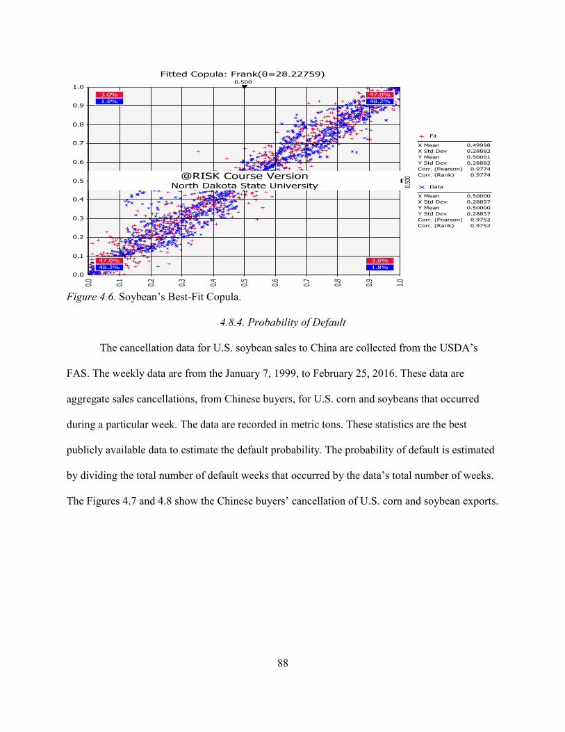
4.8.4. Probability of Default ...................................................................................... 88
4.9. Summary ......................................................................................................................... 89
CHAPTER 5. RESULTS .............................................................................................................. 91
5.1. Introduction ..................................................................................................................... 91
5.2. Analytical Model Result ................................................................................................. 92
5.3. Empirical Model Using the Stochastic Simulation’s Result ........................................... 92
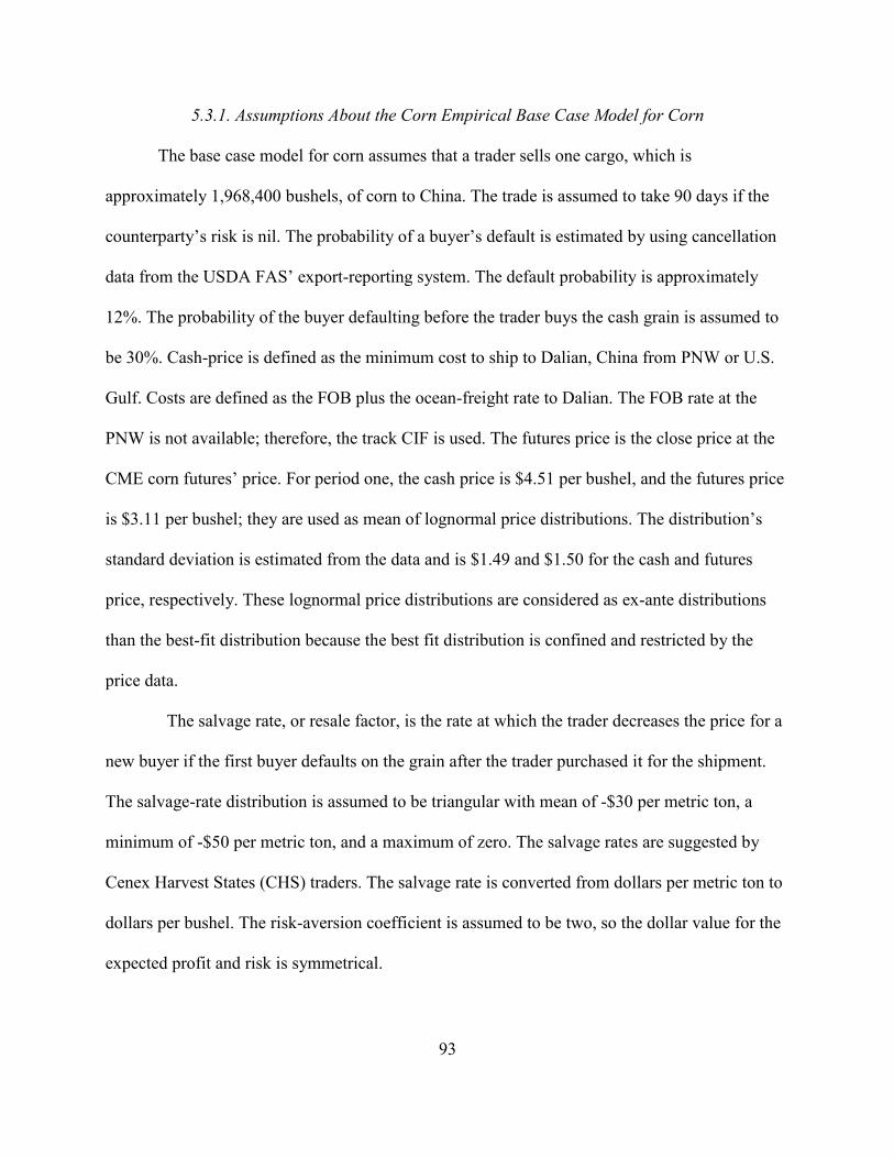
5.3.1. Assumptions About the Corn Empirical Base Case Model for Corn .............. 93
5.3.2. Base case Empirical Model Result for Corn ................................................... 94
5.4. Sensitivity Analysis with Empirical Model for Corn ..................................................... 96
5.4.1. Strike-Price Sensitivity Analysis for Corn ...................................................... 96
5.4.2. Default-Probability Sensitivity Analysis for Corn .......................................... 98
5.4.3. Before-Default Probability Sensitivity Analysis for Corn ............................ 100
Page 7
vii
5.4.4. Risk-Averse Coefficient Sensitivity Analysis (Corn) ................................... 102
5.4.5. Corn-Price Volatility’s Sensitivity Analysis ................................................. 103
5.4.6. Corn-Copula Sensitivity Analysis ................................................................. 106
5.5. Assumptions About the Empirical Base Case Model for Soybeans ............................. 107
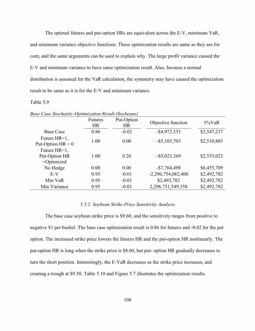
5.5.1. Base Case Empirical-Model Results for Soybeans ....................................... 107
5.5.2. Soybean Strike-Price Sensitivity Analysis .................................................... 108
5.5.2. Default-Probability Sensitivity Analysis for Soybeans ................................. 110
5.5.3. Soybean Before Default Probability Sensitivity Analysis............................. 111
5.5.4. Risk-Averse Coefficient Sensitivity Analysis (Soybeans) ............................ 113
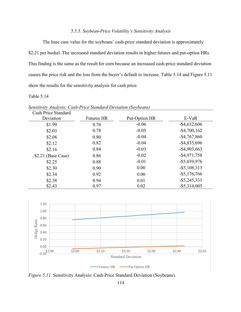
5.5.5. Soybean-Price Volatility’s Sensitivity Analysis ........................................... 114
5.5.6. Copula Sensitivity Analysis for Soybeans .................................................... 116
5.6. Summary ....................................................................................................................... 116
CHAPTER 6. CONCLUSION.................................................................................................... 119
6.1. Introduction ................................................................................................................... 119
6.2. Problem Statement ........................................................................................................ 120
6.3. Conclusions from the Theoretical Result ..................................................................... 121
6.4. Conclusions from the Empirical Results ...................................................................... 122
6.4.1. Empirical Results: Corn ................................................................................ 123
6.4.2. Empirical Results: Soybean ........................................................................... 125
6.5. Implications from the Empirical Analysis .................................................................... 127
6.6. Contribution to the Literature ....................................................................................... 128
6.7. Summary and Further Research .................................................................................... 129
REFERENCES ........................................................................................................................... 131
Page 8
viii
LIST OF TABLES
Table Page
3.1. Different Correlation Asuumptions and Optimal Hedge Ratio in Quantity Risk Models ..... 46
5.1. Base Case Stochastic Optimization Result (Corn)................................................................. 95
5.2. Sensitivity Analysis: Put-Option Strike Price (Corn) ............................................................ 97
5.3. Sensitivity Analysis: Default Probability (Corn) ................................................................... 99
5.4. Sensitivity Analysis: Probability of Default Before Cash Purchases (Corn) ....................... 101
5.5. Sensitivity Analysis: Risk-Averse Coefficient (Corn) ......................................................... 102
5.6. Sensitivity Analysis: Cash-Price Standard Deviation (Corn) .............................................. 104
5.7. Sensitivity Analysis: Future-Price Standard Deviation (Corn) ............................................ 105
5.8 Sensitivity Analysis: Copula (Corn) ..................................................................................... 106
5.9. Base Case Stochastic Optimization Result (Soybeans) ....................................................... 108
5.10. Sensitivity Analysis: Put-Option Strike Price (Soybeans) ................................................. 109
5.11. Sensitivity Analysis: Default Probability (Soybeans)........................................................ 110
5.12. Sensitivity Analysis: Probability of Default Before Cash Purchase (Soybeans) ............... 112
5.13. Sensitivity Analysis: Risk-Averse Coefficient (Soybeans) ............................................... 113
5.14. Sensitivity Analysis: Cash-Price Standard Deviation (Soybeans) ..................................... 114
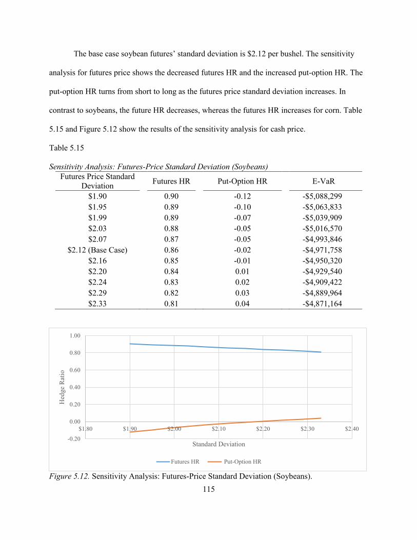
5.15. Sensitivity Analysis: Futures-Price Standard Deviation (Soybeans) ................................. 115
5.16. Sensitivity Analysis: Copula (Soybeans) ........................................................................... 116
Page 9
ix
LIST OF FIGURES
Figure Page
1.1. Default and Soybean-Crush Margins in Dalian, China ........................................................... 2
2.1. Chinese Soybean Imports and the Percentage of Imports to World Exports. ........................ 12
2.2. Cancellation of U.S. Soybean Sales to China in Metric Tons ............................................... 14
2.3. U.S. Corn Exports to China in Metric Tons........................................................................... 15
2.4. Cancellation of U.S. Corn Sales to China in Metric Tons ..................................................... 16
2.5. U.S. DDG Exports to China. .................................................................................................. 17
2.6. U.S. Sorghum Imports by China in Metric Ton..................................................................... 18
2.7. Russia’s Wheat-Export Intervention and Kansas Wheat Futures Prices ............................... 19
3.1. Synthetic Option Payoff ......................................................................................................... 70
4.1. Default Tree for the Cash Market .......................................................................................... 78
4.2. Example of the VaR ............................................................................................................... 81
4.3. Corn’s Cash and Futures Prices ............................................................................................. 85
4.4. Soybean’s Cash and Futures Prices ....................................................................................... 86
4.5. Corn’s Best-Fit Copula .......................................................................................................... 87
4.6. Soybean’s Best-Fit Copula .................................................................................................... 88
4.7. U.S.-Corn Export Cancellations by China ............................................................................. 89
4.8. U.S.-Soybean Export Cancellations by China ....................................................................... 89
5.1. Sensitivity Analysis: Put-Option Strike Price (Corn) ............................................................ 97
5.2. Sensitivity Analysis: Default Probability (Corn) ................................................................... 99
5.3. Sensitivity Analysis: Probability of Default Before Cash Purchases (Corn) ....................... 101
5.4. Sensitivity Analysis: Risk-Averse Coefficient (Corn) ......................................................... 103
5.5. Sensitivity Analysis: Cash-Price Standard Deviation (Corn) .............................................. 104
5.6. Sensitivity Analysis: Futures-Price Standard Deviation (Corn) .......................................... 105
Page 10
x
5.7. Sensitivity Analysis: Put-Option Strike Price (Soybeans) ................................................... 109
5.8. Sensitivity Analysis: Default Probability (Soybeans).......................................................... 111
5.9. Sensitivity Analysis: Probability of Default Before Cash Purchase (Soybeans) ................. 112
5.10. Sensitivity Analysis: Risk-Averse Coefficient (Soybeans) ............................................... 113
5.11. Sensitivity Analysis: Cash-Price Standard Deviation (Soybeans) ..................................... 114
5.12. Sensitivity Analysis: Futures-Price Standard Deviation (Soybeans) ................................. 115
Page 11
1
CHAPTER 1. INTRODUCTION
1.1. Overview of Study
Many risk factors in any business operation caused instability for the firm’s profitability.
The instability creates more difficulty for the firm to operate in today’s highly competitive and
risky business environment. Managing risk is one of the most important functions of the business
operation. Risk management is particularly important for commodity trading because the
industry is highly competitive and risky, and the firm or trader does not control the price for the
commodity that they are trading. The uncontrollable price fluctuation of the traded commodity is
called price risk. In order to mitigate the risk, traders hedge the price risk with commodity
derivatives that are traded at public exchanges. Also, traders can approach risk management
mathematically via the portfolio theory. The main objective of this study is to develop a hedging
model by applying the portfolio theory and to determine the optimal hedging decision for traders
who are experiencing price and default risks. There are two approaches to analyze the optimal
hedging decision. Theoretical analysis and empirical analysis. The theoretical analysis is derived,
mathematically, as the optimal hedging decision. Whereas the empirical analysis uses stochastic
optimization.
1.2. Problem Statement
Risks for commodity trading are price risk, quantity risk, weather risk, and operational
risk as well as counterparty or default risk, and many others. Two types of risks are considered in
this study: price and default risk. The price risk refers to fluctuation in the asset’s price. To
reduce the price risk, a trader hedges the commodity price with commodity derivatives such as
futures or options. The hedging is an act of taking the opposite position in similar and related
markets to reduce the price risk. When the underlying position is hedged, the loss from one
Page 12
2
market is offset by another market. Default risk is also considered in this study. The default risk
describes when the counterparty defaults on the contractual obligation. Default risk is a special
type of quantity risk has varying sizes for the quantity that is traded. Recently, the occurrence of
defaults is increasing, and traders are more cautious about the default risk in the commodity
market.
Due to a significant increase in demand for commodities, particularly in China, many
traders encountered defaults from Chinese buyers. For example, China has significant purchasing
power in the world soybean market because it is the largest buyer of world soybeans. China
imported approximately 70.40 million metric tons during the 2013 to 2014 marketing year
(Production, Supply, and Distribution). This purchasing power allows Chinese buyers to default
on soybean shipments. The soybean defaults occurred during the 2003 to 2004 marketing year
and in 2014 (Solot, 2006; and Thukral & Shuping, 2014). Figure 1.1 shows the soybean-default
and soybean-crush margins in China’s Dalian region (Thomson Reuter Eikon 2016d). The figure
illustrates that a lower soybean-crush margin increases the chance and number of cancellations.
Figure 1.1. Default and Soybean-Crush Margins in Dalian, China.
-400
-300
-200
-100
0
100
200
300
400
500
600
0
100000
200000
300000
400000
500000
600000
700000
800000
6/2/2010 6/2/2011 6/2/2012 6/2/2013 6/2/2014 6/2/2015 6/2/2016
Cancellation Soybean Crush Margin Breakeven
Page 13
3
Similarly, corn and distiller dried grain (DDG) are defaulted by many Chinese buyers due
to the import ban of MIR162 varieties in late 2013 to 2014(“China Rejects,” 2013; Farm City
Elevator, Inc., 2014). Corn and DDG are one of many cases of defaults that occurred with in
agricultural products. Many other instances of defaults are seen not only in agricultural products,
but also for other commodities. 1
As an illustration to see the default’s effect on the trade’s profit and loss, suppose that a
trader sells grain to an overseas buyer and hedges the entire sale with a futures contract. In this
case, the trader has a short position in the cash market and a long position for the futures market.
Suppose that the price declined, causing the buyer to default on the purchase contract. The
default worsens situation because the loss from the futures position is magnified by a decreased
return for the cash position. The futures contract has a limited ability to hedge both the price and
default risks. Therefore, we introduce a put option to the hedging model in order to, primarily,
hedge the default risk.
1.3. Portfolio Model of Hedging
Portfolio theory originates from Markowitz’s (1952) seminal paper. One of the main
objectives is to determine the optimal allocation for a risk-averse investor who is considering the
portfolio’s expected and variance return. When portfolio theory is applied to hedging for
commodities, its main objective is to find optimal HR for the futures and option to either
1 Although this thesis addressed the buyer’s default risk with international trading, similar problems exist for the
seller’s risk in some countries. As an example, the following message was received from a trader who worked with
the former Soviet Union (FSU):
We started this year to actively originate and sell third party grain. Since June, we have purchased 650,000
tons for $100 million. In 2017, we want to trade 2 million tons for $300 million.
While we measure and manage the price risk of our open trading position through a VaR calculation, I am
concerned about our counterparty risk. For example, we buy grain forward from Ukrainian farmers and
sell it forward to international traders. If grain prices spike in the meantime, farmers might default and we
sit on losses, which our trading margin cannot cover. We therefore need to implement a system to measure
and manage counterparty risk (Wilson, W., W., personal communication, October 31 2016)
Page 14
4
maximize or minimize the objective function. Researchers can specify several objective
functions. This study includes but not limited to minimum variance, mean-variance (E-V),
semivarinace, lower partial moments (LPM), mean-Gini coefficient, minimum value-at-risk
(VaR), and mean-VaR (E-VaR). In this study, the E-V and E-VaR are used. Each objective
function has advantages and disadvantages. For example, variance minimization is utilized to
reduce the portfolio’s variance. Similarly, the E-V framework maximizes the risk adjusted
expected return function which approximates the trader’s utility. The variance treats upside and
downside risk equally. The equal treatment is the biggest disadvantage of using variance to
measure risk because a risk averse trader prefers upside over downside risks. In contrast to
variance, VaR is a downside risk measure and only considers the downside risk. This study
focuses on E-V and E-VaR for the theoretical and empirical approaches respectively.
Traditionally, portfolio-hedging models assume a known cash position and only hedge
with a futures contract. However, default risk is special type of quantity risk, and for this reason
we have a put option in the study’s objective function. The default risk is incorporated in the
model by assuming that default risk has a probability distribution. Including put options offers
more flexibility for hedging, and the asymmetric payoff allows the trader to hedge more
efficiently hedge default risk. Integrating the default risk and put option with the hedging
model’s development is a major improvement compared to the traditional hedging model.
1.4. Theoretical Approach
A theoretical hedging model which incorporates the default risk and includes the futures
and put options is specified. Constructing the theoretical model is based on Bullock and Hayes’
(1992) paper. The theoretical model uses the E-V framework. The cash, futures, and default
distributions are assumed to be normal. In order to derive the first and second moments of profit,
Page 15
5
Bullock and Hayes’ (1992) theorem is applied. This theorem allows us to split the total payoff
function at strike price of the put option. This theorem is useful to bypass the problem caused by
the put option’s asymmetric payoff. The major result from the theoretical analysis is the
existence of a global optimum solution that maximizes the E-V function. Global optimum is
proved by showing that the optimal futures and put option HRs exist and that the Hessian matrix
is negative definite. This result is powerful because, at least theoretically, a solution exists.
1.5. Empirical Approach
The empirical analysis uses Monte Carlo simulation and stochastic optimization to
estimate the optimal HRs under default risk. This analysis is conducted for soybeans and corn.
The price distributions are lognormally distributed, and the default risk is assumed to be a
Bernoulli distribution. The E-VaR is utilized as the objective function because using the VaR as
a risk measure is appealing. The E-VaR is appealing because it has an expected profit component
while, the VaR is a downside risk measure. The base case optimization result is derived to create
a standard for analysis. Alternative hedging scenarios and different objective functions are
assumed in order to compare the optimization results. Additionally, sensitivity analyses are
conducted to see the effect of changing the variable’s value and the correlation assumption to the
optimization result.
From this analysis, traditional naïve hedging is a suboptimal hedging strategy, and
surprisingly, the alternative objective functions lead to the equivalent optimization result.
Another important result comes from using the copula function instead of the Pearson linear-
correlation function. Copula leads to more realistic optimization results because the copula
preserves correlation structure between random variables.
Page 16
6
1.6. Thesis Organization
This thesis is organized as follows. Chapter 2 is the review of the related literature and
the background of the problem. The chapter discusses defaults for both agricultural and non-
agricultural markets as well as the academic literature for the hedging’s portfolio model and its
findings. Chapter 3 explains the theoretical model. The chapter focuses on mathematical
constructions of the different hedging models and developing the theoretical model for analysis.
Chapter 4 contains a detailed explanation about the empirical model and the data used for the
analysis. In Chapter 5, both the theoretical and empirical Results are presented and discussed.
Chapter 6 contains the study’s Conclusions and implications.
Page 17
7
CHAPTER 2. LITERATURE REVIEW
2.1. Introduction
Risk management is one of the paramount aspects of running successful agribusinesses.
The managers can reduce risk by taking the opposite position for a commodity derivative such as
futures or options in related markets to reduce the risk of physical-commodity price changes. The
study’s main focus is to derive the optimal HR by considering the existence of one of the
counterparties’ default risk. In commodity marketing, the default risk is a special case of
production, or quantity, risk. If the buyer defaults on the agreed sale, the seller gains zero
revenue. However, quantity risk can be hedged with commodity derivatives by taking the
position based on portfolio-hedging models. The HR is the futures or options position that is
taken with respect to the cash position’s size. For example, if the HR is one, the size of the
futures or option contract is equal to the cash position’s size. In order to find the optimal HR, the
hedger first needs to think about the definition of the risk for moving forward.
2.2. Risk in Agriculture and Commodity Marketing
In this study, the definitions for risk and uncertainty are treated differently to evaluate the
default risk’s effect on the HR. A risky event has probabilistic outcome whereas uncertainty is an
event that cannot be associated with probability (Chavas, 2004). In other words, a risk has an
associated probability distribution, but uncertainty does not have probability distribution. This
distinction is important to analyze the default risk’s impact on the optimal HR. Difficulty arises
when the default event is uncertain because without knowing the likelihood of a default, building
an analytical model is almost impossible. Because risk and uncertainty are defined, we first
review the most common forms of risk in agriculture.
Page 18
8
The most notable risks in agriculture are related to price and quantity. Price risk
originates from fluctuating commodity prices. By definition, the price risk has associated
probability distributions; therefore, the price risk can be measured by using the standard
deviation or variance of a commodity’s historical price or return during a specified time period.
A higher price risk means greater standard deviations, and lower a price risk means lower
standard deviations. Farmers and producers are subject to significant price risks if the cash
market in which they participate has a high standard deviation for the price. For farmers,
understanding of the behavior of the cash market where that they participate is a critical element
of risk management (Tomek & Peterson, 2001). Farmers hedge the price risk of their cash
position by using the commodity futures and options that are traded at centralized exchanges,
such as the Chicago Board of Trade (CBOT), or take forward contract to set a delivery price and
time. Without considering the basis risk, transaction cost, and storage cost, the farmer can hedge
the entire cash position, which implies a HR of one, by selling an equal amount of futures in the
futures market. The HR of one removes the return fluctuation that is caused by the physical
commodity’s price movement if the basis risk is zero. Any loss incurred from the cash position
due to a decreased price is offset by profit from the short futures position and vice versa.
Similar to the price risk, yield risk arises from the quantity’s fluctuation. This risk is felt
by a commodity’s farmers or producers and leads to revenue fluctuations. When a farmer hedges
the price risk using futures and options to obtain more stable revenue, he/she has difficulty
determining the hedging position’s optimal size due to yield risk. They end up either under-
hedging or over-hedging relative to the actual production at the end of harvest period. If the
producer under-hedges or over-hedges compared to the actual harvest, the hedge may not be
optimum.
Page 19
9
2.3. Forward vs Futures Contracts
There is difference between a forward contract and a futures contract. Both forward and
futures contracts are agreements between buyers and sellers. A forward contract is an agreement
between two parties for the delivery of product at a specified future date and price which are
written in the contract (Kolb & Overdahl, 2007). In contrast, a futures contract is a highly
standardized type of forward contract with more specified contract terms (Kolb & Overdahl,
2007). Moreover, the futures contract is subject to the margin mechanism and clearinghouse
procedures that do not exist with the forward contract. The futures contract has margin
mechanism and counterparty risk is eliminated by clearinghouse.
The biggest difference between a forward and futures contract is that a forward contract
is subject to the counterparty’s default while the futures contract is not. The forward contract is
subject to default risk because there are no or limited guarantees in the agreement. Default risk
exists because the forward contract is done privately without a clearinghouse; at the same time,
because the agreement is done privately, the contractual terms and specifications are negotiable.
The reason why a futures contract is not subject to default is because the futures trading goes
through organized exchanges such as the Chicago Mercantile Exchange(CME), and are required
to go through a clearinghouse. The clearinghouse’s job is to assure that every trader who
participates in the futures trading honors the obligation. The clearinghouse matches the position
of every buyer to every seller and the position of every seller to every buyer, and every trader in
the market only has an obligation to the clearinghouse (Kolb & Overdahl, 2007). In addition to
trading through the clearinghouse, traders must deposit money with a broker when they initiating
trade in the futures market. This deposit, the margin, is a financial protection which forces the
trader to follow the contractual agreement (Kolb & Overdahl, 2007).
Page 20
10
2.4. Defaults in Commodity Marketing and Trading
Many risk types exist in the production and marketing of agriculture. They include yield
and price risks. Default risk, or counterparty risk, has become more prevalent in agricultural
marketing and commodity trading in general; hence, traders and risk managers find it necessary
to hedge counterparty’s default risk, i.e., contract non-performance risk. This section is an
overview of defaults instances for agricultural and non-agricultural backgrounds.
2.4.1. Definition of Default
The first step in risk management is to clearly define the risk. The default risk is when
one of the parties involved with a transaction reneges on the obligation. Jarrow and Turnbull
(1995) identify two sources of default risk. The default occurs when payment is less than agreed
payment or the writer of the derivative security defaults (Jarrow and Turnbull, 1995). Zhu and
Pykhtin (2007) have similar definition that the counterparty credit risk is when the counterparty
defaults before the contract matures and does not make all the promised payments.
2.4.2. Types of Counterparty Credit Risk
In this study, two types of counterparty credit risk exist in agriculture. The first type is a
strategic default by one of the parties, and the second type is a non-strategic default. The
difference between these two defaults types is simple. A strategic default occurs when defaulting
on the purchasing contract is more beneficial than honoring the original contract. Historically,
the strategic default occurs when market volatility increases tremendously. Non-strategic default
takes place when exogenous, uncontrollable, factors, such as an import or export restriction,
cause the counterparty to default on the purchasing and sales contracts. These default types are
the dominant ones that occur in the commodity marketing and trading.
Page 21
11
2.4.3. Impact of Defaults on Traders
The default’s impact on the commodity traders is large because of a synergizing effect
that comes from both the cash and futures positions. As an example, a U.S. based commodity
trader sold soybeans to a crusher in China for $10 a bushel. The trader in the United States is
short cash, and the trader hedges the short-cash position with a long-futures position. Suppose
that the soybean price drops to $5 bushel, and that the buyer defaults on the contract. The trader
has to find new buyer for the cash commodity at lower price than the originally agreed-price also
losing the profit from the long-futures position ($5 bushel in this example). This simple example
illustrates where the loss is synergized rather than offsetting because no return is coming from
the cash position.
2.4.4. Chinese Buyers Defaulting on Soybean
The defaults for the grain-procurement agreement have become more prevalent in the
agriculture sector, especially for international commodity trading. The most well-known default
case for international commodity trading is by China’s soybean buyers. Historically, China is the
world’s largest importer of soybeans. According to the Foreign Agricultural Service (FAS) at
United States Department of Agriculture (USDA), China imported 70.364 million metric tons
during the 2013 to 2014 marketing year, and this is approximately 62 percent of total world
soybean export (U.S. Department of Agriculture, Foreign Agricultural Service, 2015c). The
amount imported by China is almost six times greater than the second largest soybean importer,
European Union, of 12.538 million metric tons in 2013/2014 marketing year (U.S. Department
of Agriculture, Foreign Agricultural Service, 2015c). Due to the amount of soybeans that China
imports each year, the country has huge buying power and advantages when buying soybeans
Page 22
12
from the world market. Figure 2.1 shows Chinese soybeans imports and its percentage compared
to total world export.
Figure 2.1. Chinese Soybean Imports and the Percentage of Imports to World Exports.
During the early 2000s, the soybean-crushing margin, the profit margin for crushing
soybeans, in China was considerably high, but the margin decreased when the soybean price
started rising. The margin turned and stayed negative during 2003 and 2004 (Solot, 2006). In
April 2004, many Chinese soybean crushers contracted to purchase soybeans at $10 a bushel;
however, during the delivery time in June to August, the price of soybean dropped to $6 a
bushel, which leading to a default on the contract (Solot, 2006).
In 2014, some Chinese soybean buyers defaulted on soybean cargo because they failed to
obtain a letter of credit, a document which is issued by a bank to guarantee that the seller
receives full payment when the delivery condition is fulfilled. One goal for letter of credit is to
reduce credit risks. When a buyer is unable to fulfill the purchase’s payment, the bank steps in
and pays the outstanding amount. Because Chinese importers could not obtain letter of credit
from banks and had losses with soybean crushing, the Chinese importers defaulted on at least
57%
58%
59%
60%
61%
62%
63%
64%
65%
0
10000
20000
30000
40000
50000
60000
70000
80000
90000
2011/12 2012/13 2013/14 2014/15 Jun 2015/16 Jul 2015/16
China Soybean Imports Percentage of Import to World Exports
Page 23
13
500,000 tons, approximately $300 million, of the U.S. and Brazilian soybean cargo; this action
was the biggest default that occurred since 2004 (Thukral & Shuping, 2014).
The Chinese soybean buyers’ 2014 default case raises questions about why soybean
exporters did not confirm the letters of credit before signing a purchasing agreement. After the
2004 default, soybean exporters stopped shipping soybeans to China without confirming the
importer’s letter of credit. This practice slowly started again and lead to the 2014 default case
(Thukral & Shuping, 2014). Also, some trading firms relaxed the letter-of-credit requirement and
accepted deposits from clients, particularly clients with well-established relationships (Topham
& Shuping, 2014). With China’s 2014 soybean default, some soybean cargo changed the
destination of ocean shipping after the default incident. The two soybean shipments that were
sold by the Japanese trading firm Marubeni Corp. contained Brazilian soybeans that were headed
to China: those soybeans were rerouted to the United States (Plume, 2014).
The cancellation was derived from the USDA’s export-sales reporting system, an export
sales reporting program which monitors the 39 commodity sales made to foreign country from
the United States on a daily and weekly basis. Commodity exporters are required to report the
sale of more than 100,000 metric tons of a commodity to a single destination per day or more
than 200,000 metric tons of total sales for single commodity to the one destination in a reporting
week (U.S. Department of Agriculture, Foreign Agricultural Service, 2015a). These data are a
proxy to illustrate the amount of cumulative sales cancellations for a single commodity that
occurred during a particular week. Figure 2.2 represents the cancellation of U.S. soybean sales
that were destined for China from 1990 to 2016.
Page 24
14
Figure 2.1. Cancellation of U.S. Soybean Sales to China in Metric Tons.
Since 2005, there was an upward trend for China’s cancellation of U.S. soybean sales: the
peak was in 2012. From 2013 to 2015, the cancellation level stayed above 2 million metric tons.
Although soybean exporters may incur losses from Chinese soybean importers’ defaults, the
Chinese soybean market is the most lucrative one in the world due to the country’s quantity of
soybean imports. Because of the quantity of China’s imports, Chinese soybean buyers have
strong negotiating power over the commodity-trading firms that sell to China. Therefore, credit
risk management is becoming more important in the world of commodity trading. According to
personal communication with W. W. Wilson Chinese buyers purchased the U.S. soybeans
exported from New Orleans, Louisiana region around $1.10 to $1.35 basis price. The soybeans
basis price dropped to $0.28 due to cheap ocean freight rate and the competition from Brazil, the
Chinese buyers may default on the original soybean contract (personal communication,
November 23, 2016).
28197 18205
382230
619997
350708
1695845
122362
350071
895937
1295807
2042720
1833336
2722926
3029120
2157842
23736282314140
218084
1999 2000 2001 2002 2003 2004 2005 2006 2007 2008 2009 2010 2011 2012 2013 2014 2015 2016
Page 25
15
2.4.5. MIR162 Corns, DDG, and Sorghum Exports to China
The United States produced approximately 351 million metric tons of corn, 36% of the
world’s corn production, during 2013 to 2014 crop year (U.S. Department of Agriculture,
Foreign Agricultural Service, 2015c). In terms of the corn trade, China is not as large of an
importer as with soybeans. China imported 3.277 million metric tons of corn in the 2013/2014
crop year (U.S. Department of Agriculture, Foreign Agricultural Service, 2015b). Although
China does not import as much corn as it does soybeans, China significantly influences the
world’s corn market. Figure 2.3 shows U.S. corn exports to China.
Figure 2.3. U.S. Corn Exports to China in Metric Tons.
A major default case for the corn market is an import rejection of U.S. corn by the
Chinese government due to an unapproved genetically modified (GM) trait that was found in
imported corn. This specific, unapproved GM corn found was SYN-IR162-4, the so-called
MIR162 trait, developed by Syngenta Seeds, Inc. The MIR162 corn for approved in major corn
markets, except China, and the first rejection of the U.S. corn occurred on November 18, 2013
0
100000
200000
300000
400000
500000
600000
700000
800000
900000
2012-2012 2013-2013 2014-2014 2015-2015
Page 26
16
(Farm City Elevator, Inc., 2014). According to the weekly report published by Informa
Economics (2014), the purpose of restricting GM corn is to increase the consumption of China’s
domestic corn. The landed value of the U.S. corn in China is significantly cheaper than China’s
domestic-government-supported corn price which incentivizes consumers to purchase other
overseas grains for feedstuffs. Figure 2.4 shows the cancelation of the U.S. corn sales to China
from 1999 to 2016 in metric tons. In 2014, there was a huge spike in the cancellation of U.S.
corn, primarily because of the MIR162 trait’s rejection by the Chinese government.
Figure 2.4. Cancellation of U.S. Corn Sales to China in Metric Tons.
In addition to the U.S. corn exports that were affected by the China’s import rejection due
to the unapproved MIR162 varieties, the byproduct of corn crushing, which is called distillers’
dried grain (DDG), and sorghum exports to China also affected by rejections. DDG is a
byproduct of ethanol which is produced with a process called crushing. The physical crushing is
the process of converting corn into ethanol and DDG. Usually, DDG is used for a livestock feed
1 0 0
885000
0 0 25540 8106 0 0 0
242456
899
643899
819129
2767627
993500
1999 2000 2001 2002 2003 2004 2005 2006 2007 2008 2009 2010 2011 2012 2013 2014 2015 2016
Page 27
17
because it is a rich, high-protein source. On December 27, 2013, Xinhua reported that two
batches, approximately 758 tons, of the U.S. DDG with soluble were rejected because Chinese
officials found them to contain the MIR162 strain (“China Rejects”, 2013). Because MIR162
corn varieties are unapproved GM varieties, China imposed inspection of DDGs imports in July
2014, and any shipment with DDG purchases after August 18th is required to have MIR162 free
certificate (Informa Econmics, 2014). Chinese authorities’ inspection apparently caused a
decrease in the U.S. DDG exports to China as which is shown in the Figure 2.5 (United States
Department of Agriculture, Foreign Agricultural Service, 2015b).
Figure 2.5. U.S. DDG Exports to China.
After the import ban for U.S. corn and the DDG inspection, U.S. sorghum exports to
China increased more than 15-fold in 2014, and some Kansas grain elevators offer a 10%
premium for sorghum above the corn price because sorghum does not have a futures market and
because corn is used as reference for sorghum prices (Kesmodel, 2015). This phenomenon
indicated that sorghum is a substitute for China’s corn-import demand. Chinese importers moved
0
100000
200000
300000
400000
500000
600000
700000
800000
900000
1000000
2012-2012 2013-2013 2014-2014 2015-2015
Page 28
18
their interest to purchase U.S. sorghum as an alternative, cheaper feedstuff, and the U.S.-corn
import restrictions likely had a positive impact on U.S. sorghum exports to China (Informa
Economics). The Figure 2.6 shows the increase in U.S. sorghum imported by China (United
States Department of Agriculture, Foreign Agricultural Service, 2015c).
Figure 2.6. U.S. Sorghum Imports by China in Metric Ton.
Because the imported U.S. corn contained unapproved MIR162, there were many
interesting consequences for corn, DDG, and sorghum. MIR162 corn was approved by Chinese
officials during at the end of 2014. On December 22, 2014, Syngenta announced that MIR162
received formal import approval from China’s regulatory authorities (Syngenta AG, 2014).
2.4.6. Defaults for the Wheat Market
Another major loss in the grain market is caused when one of the largest wheat-exporting
countries, such as the Russian Federation, bans grain exports and establishes quotas. This
decision has effects on wheat importers because they may have to find a new seller with a higher
price. According to the U.S. Wheat Associates (2011), governments’ export bans cause
contractual prohibition and cancellation, creating a higher price than originally agreed upon for
importers. Russia is known for banning grain exports, particularly in 2010, to deal with poor
0
2000
4000
6000
8000
10000
12000
2011/12 2012/13 2013/14 2014/15 2015/16Jun 2015/16Jul
Page 29
19
production due to drought and rising food prices. Additionally, Russia changed the tariff rates for
wheat that was exported overseas (Blas, 2010; Global Agricultural Information Network, 2014;
Kolesnikova, 2010; Kramer 2010; Vassilieva & Pyrtel, 2007). Because Russia is one of the
largest wheat producers, a buyer is forced to find a different wheat seller. In 2010, Many Russian
wheat buyers had to find an alternative seller with price that was $100 per metric ton above the
original purchase price (U.S. Wheat Associates, 2011). According to the U.S. Wheat Associates
(2015) Russia’s state intervention creates extreme price volatility which is shown in Figure 2.7.
The figure shows the effect of five Russian interventions from 2007 to 2014, on the Kansas
wheat-futures price. The increases were as follows: 30% in two 2014 interventions, 45% with the
2012 intervention, and 100% for the 2007 and 2008 interventions (U.S. Wheat Associates, 2015).
Figure 2.7. Russia’s Wheat-Export Intervention and Kansas Wheat Futures Prices.
An extreme price move causes a supplier to default on the agreed selling contract. In
2012, the rise in the global commodity prices, triggered by a drought in the United States
Page 30
20
incentivized grain suppliers to default on the delivery contract because that contract created a
loss from rising commodity prices (Hogan & Saul, 2012). With international grain trading, there
is a function to force an agreement between counterparties. Most international grain contracts
requires as 10% performance bond which the seller has to pay to buyer when a contract default
occurs (Hogan & Saul, 2012). With a 10% performance bond, the seller defaults when better
than keeping original agreement (Hogan & Saul, 2012). Defaulting on the sales contract may
have a negative influence on the long-term relationship, but with extreme price movements
defaulting on the sales agreement may be more beneficial for suppliers.
2.4.7. Defaults for the Cotton Market
An incidence of supplier default happened with cotton trading due to an unexpected price
rise in the global cotton market. According to Pirrong (2014) and Kub (2012), the cotton
market’s contract performance risk emerged in during late 2010 to 2011. At that time, the world
cotton price tripled, which led sellers to default on physical purchasing contracts; also when
prices came back down, consumers defaulted on the contracts (Kub, 2012; Pirrong, 2014). With
this unexpected rise in the cotton price, Glencore suffered when suppliers defaulted on
purchasing contracts and had to purchasing cotton at a higher price (Kub, 2012).
2.4.8. Non-Agriculture Default Cases
A similar default case happened with the iron-ore and coal trade in China. According to
Wong and Fabi (2012), there were at least six coal-cargo defaults as well as defaulting iron-ore
contracts because of the price drop. Wong and Fabi (2012) said that the default was sparked by
the drop in global, thermal coal benchmark prices to two-year lows and the increased
anticipation of a steeper fall for the benchmark price. The comment made by a Singapore-based
Page 31
21
iron-ore trader in Wong and Fabi’s (2012) article was a typical example of a buyer defaulting on
a contract when the price is fell:
We ourselves have had one of our buyers default on us after just a few hours. We sold the
cargo to an end-user in China and a few hours later the buyer came back, saying “the
market’s falling too fast we want a lower price’.” (p. 2)
We analyzed the default cases in both the agricultural and non-agricultural markets, and
cancellation and default were not uncommon events. In the next section, an overview of the
portfolio model of hedging is discussed.
2.5. Portfolio Hedging Models
The conceptual framework used to determine the optimal HR builds on portfolio
optimization or the so-called modern portfolio theory, which was first published in Markowitz
(1952). This model focused on the fact that investment’s future return is dependent on the
selection of the portfolio by considering the expected return and the variance of return as
portfolio’s desirable and undesirable aspects, respectively. With an analytical model that has
finite number of securities, Markowitz (1952) formulated an investment rule called the expected
return – variance of return (E-V) rule. This rule states that an investor chooses an efficient
portfolio from a set of possible combinations for the portfolio’s expected return and variance.
This rule implies that an investor can select a portfolio by considering its E-Vs. Therefore, the
investor can select a portfolio with the minimum variance of return or can accept more return
variance to obtain a higher expected return. E-V is the portfolio’s risk-return tradeoff. Hedging
the cash position with futures and options by determining the optimal HR is the portfolio
optimization, and there are different approaches to use when setting the objective function.
Page 32
22
In order to calculate the optimal HR, both the theoretical framework and estimation
procedures of the optimal HRs are important. Many of the HR’s theoretical models are different
and based on the objective function’s maximization or minimization. The portfolio hedging
models can be classified as minimum variance, utility maximization, and risk-adjusted return
functions. With the minimum-variance hedging model, the hedger selects a HR that minimizes
return’s variance. Under the utility-maximization framework, the objective is to maximize the
utility. The risk-adjusted return is similar to the expected utility maximization; however, risk-
adjusted return is not associated with any specific utility functions.
2.5.1. Minimum-Variance Hedging Model
The minimum-variance hedging model does not reflect the return which the hedger seeks
from the selected portfolio. With the portfolio theory of hedging, the position in the cash market
is fixed, and the hedger has required to decide how much of the fixed cash position should be
hedged (Ederington, 1979). Johnson (1960) developed a minimum-variance hedging model and
theoretically analyzed how the hedger takes a position in the futures market to reduce the
portfolio’s variance of return which is caused by the commodity’s price risk. Similarly,
Ederington (1979) developed the minimum variance hedging model and conducted an empirical
analysis assuming cash position in the Government National Mortgage Association’s (GNMA)
8% Pass-Through Certificates, Treasury-Bill (T-Bill), wheat, and corn, and these were hedged
with corresponding futures contracts. Both Johnson (1960) and Ederington (1979) derived the
optimal HR from the variance of return equation, which is the ratio of the covariance of the spot
and futures market, and the variance of the futures market. The derived, optimal HR equation
was extended to formulate a measure of hedge effectiveness. The hedge’s effectiveness is
measured by the square of the correlation the spot and futures market. If the correlation for the
Page 33
23
commodity’s price movement in the spot and futures market is one, the loss from one market is
exactly offset by the profit made from the other market (Johnson, 1960). With this measure of
hedge effectiveness, the lower the correlation for the price movement in the spot and futures
market is an indication of a bad hedge because the loss from the spot market due to adverse price
movement may not be offset by the profit made with the futures market. Ederington (1979)
found that GNMA futures market was a more effective hedging instrument than the T-Bill
market for risk-avoidance purposes.
2.5.2. Mean-Variance Hedging Model
Instead of only focusing on minimizing the portfolio’s variance, the E-V model focuses
on both the portfolio’s expected return and variance to determine the optimal HR. One may
consider that the minimum-variance HR is just a special case of the E-V HR. The minimum-
variance HR is consistent with the E-V framework when the hedger is infinitely risk averse or
when the expected futures’ price change is zero. When the expected future price change is zero,
it is pure martingale process (Chen, Lee, & Shrestha, 2003). Many studies incorporate the E-V
approach to find the optimal HR (Blank, Carter, & Schmeising, 1991; Cecchetti, Cumby, &
Figlewski, 1988; Howard & D’Antonio, 1984; Hsin, Kuo, and Lee, 1994). These studies are
utility maximization under the E-V framework which aims to enhance the minimum-variance
hedging model. With the E-V framework, the utility function, which the hedger is willing to
maximize, is defined in terms of the expected return and variance for the hedged portfolio.
Because only the first two moments of distributions are involved with the E-V utility function, E-
V framework can be easily applied for risk analysis (Chavas, 2004).
The theoretical, optimal HR was derived in Blank et al. (1991): it maximized the
expected utility of the hedger and included the expected return and variance for the hedged
Page 34
24
portfolio as well as the hedger’s risk-aversion parameter. From this optimal HR formula, Blank
et al. (1991) concluded that the formula had two sources of demand for the futures: hedging
demand and speculative demand. The hedging demand for the utility-maximizing HR was the
same as the minimum-variance HR, and the speculative demand showed hedger’s expectation for
the hedge’s return because for speculative demand formula includes hedger’s risk parameter
(Blank et al., 1991). Blank et al.’s (1991) approach was the utility-maximization approach under
the E-V framework where the hedger tried to maximize the utility based on the mean, variance,
and risk aversion parameter.
Because many researchers illustrated the unrealistic nature of minimum variance
hedging, Cecchetti et al. (1988) argued that the minimum-variance hedge was not optimal
because it did not consider the expected return and the time-varying distribution of the spot and
futures prices. Cecchetti et al. (1988) assumed that the hedger had log utility and tried to
maximize the expected-utility function with the time-varying joint distribution of spot and
futures returns which is estimated using the autoregressive conditional heteroskedasticity
(ARCH) model. Cecchetti et al. (1988) also argued that the hedge effectiveness should be
measured in terms of the expected utility or the return from the certainty-equivalent. Using the
empirical result based on hedging the 20-year Treasury bond in the post-sample and in-sample
periods, Cecchetti et al. (1988) found that log-utility maximization is better than the minimum-
variance hedge when they compared the returns’ certainty-equivalent.
Hsin et al’s (1994) model hedges the currency exchange-rate risk with the currency’s
futures and options. Under the assumptions of the negative-exponential utility function, hedger’s
constant absolute risk aversion (CARA) and the normal return distribution, the expected utility
maximization depends on the utility function with portfolio’s mean and variance (Hsin et al,
Page 35
25
1994). Additionally, Hsin et al. (1994) measured the hedge effectiveness as the difference
between the certainty-equivalent of the hedged and spot position. Hsin et al. (1994) conducted an
empirical study and concluded that the currency futures are a better hedging tool than the
currency options regardless of whether the options are synthetic futures or delta/gamma hedges.
Under the E-V framework, Howard and D’Antonio’s (1984) approach includes the risk-
free return in the expected utility function. This approach is rather unique approach compared to
other approaches. The hedger can hold a risk-free asset in the hedged portfolio to reduce the
portfolio’s risk. The purpose of holding futures position is not solely on the reduce portfolio risk,
but it also aims to improve the risk-return characteristic (Howard & D’Antonio, 1984).
Therefore, the hedger maximizes the utility function which depends on the differences for the
expected return from the spot and futures positions, the return from the risk-free asset, and the
portfolio’s standard deviation for spot and futures positions (Howard & D’Antonio, 1984). The
major finding from Howard and D’Antonio’s (1984) is risk-return relative. The risk-return
relative shows spot and future relative return attractiveness. The relationship between risk-return
relative and the correlation for spot and futures prices show is important. This relationship
defines the hedger’s activity taking a futures position. If the risk-return relative is greater than the
correlation, the hedger long futures contract. If risk-return relative is smaller than correlation
coefficient, the hedger shorts futures contract. If risk return-relative is equal to the correlation
coefficient, the hedger does not hold any futures position (Howard & D’Antonio, 1984).
The expected utility-maximization approach starts with an assumption for the utility
function. Lence (1995, 1996) investigated the value of better approximation for the minimum-
variance hedge by maximizing the expected utility of the risk-averse hedger’s terminal wealth.
One of Lence (1995, 1996) contributions was relaxing the assumptions that are ignored by most
Page 36
26
hedging literature: including the transaction cost and margin requirement. Additionally, Lence
(1995, 1996) assumed that the hedger can borrow and lend capital and can also invest his/her
own capital into an investment, yielding a certain return. Both Lence (1995, 1996) measured
hedge effectiveness in terms of the hedger’s opportunity cost to select a suboptimal return
instead of the optimal return. Lence (1995) assumed that the distributions for the return from
spot, futures, and alternative investment were joint normal distributions and that the utility
function was CARA. Lence (1995) conducted a simulation of the hedger’s behavior, considering
the estimation risk, and found that value of better estimation for the minimum-variance hedge is
insignificant and that the minimum variance hedge with a relaxed assumption resulted in the
optimal hedge being significantly different than the usual assumptions. Lence (1996) relaxed the
assumptions made in Lence (1995), one by one, to see the effect of changing the minimum-
variance hedge’s value. The biggest assumption changes made from Lence (1995) to Lence
(1996) were stochastic production and not allowing all initial wealth to be invested into
production. From the simulation results, Lence (1996) concluded that, with increased risk-
averseness, the stochastic production reduced the optimal HR and the opportunity cost of not
hedging at all to futures. The alternative investment opportunity induced the optimal HR to be
proportional to the correlation between the alternative investment and futures prices.
2.5.3. Mean-Value-at-Risk Framework
E-VaR is a framework that adjusts the expected return with portfolio’s VaR. The
objective function is classified as risk-adjusted return function. This framework is gaining
popularity for portfolio selection and hedging. This framework is used for the empirical analysis
in Chapter 4. One of the early studies using E-VaR was conducted by Alexander and Baptista
(2002). They compared the E-VaR portfolio selection to E-V, assuming a multivariate normal
Page 37
27
distribution of assets. Alexander and Baptista (2002) concluded that, as the VaR confidence
interval increases, the minimum VaR converges to the minimum variance while the E-VaR
converges to E-V. Alexander and Baptista (2002) also proved that E-VaR approximately
maximizes the expected utility of a risk-averse agent.
When hedging, Awudu, Wilson, and Dahl (2016) used the E-VaR framework to hedge
input and output price risks for ethanol. Using a stochastic optimization, they determined the E-
VaR maximizing HR for three different hedging strategies: short corn, long corn, and hedging
the crush margin. With the short-corn strategy, the producer sold all outputs and was left to buy
corn. The long-corn strategy assumes that corn was purchased and that the output was sold as
futures. The third strategy was to hedge the crush margin. With this strategy, the producer did
not sell output and, instead, purchased inputs. The optimization result concluded that short corn
was the best strategy because it had the highest E-VaR value.
2.5.4. Other Hedging Frameworks
For the E-V analysis to be consistent with the expected utility-maximization principle,
restrictions need to be imposed on the utility’s function and return distribution. Chen et al.
(2003) stated that the utility function had to be a quadratic function and that the return’s
distribution to be a normal distribution. If these assumptions were not made, then the HR may
not be optimal with respect to the expected utility-maximization framework (Chen et al., 2003).
All types of hedging paradigms, the minimum-variance hedge, E-V, expected utility
maximization, and risk-adjusted return have strengths and weaknesses. Minimum variance only
focuses on the hedged portfolio’s variance. E-V approach has a restriction for the utility function
and the return’s distribution to be consistent with the expected utility maximization. The E-V
framework is negative utility function. Therefore, one of the most important specifications is the
Page 38
28
utility function and for the portfolio’s return distribution. Considering the restrictive assumptions
about the hedging models mentioned so far, there is high demand to develop a hedging model
which has less-restrictive assumptions about the hedger’s utility function and return distribution.
Hedging models which lessens assumptions about specific utility functions and the
return’s distribution utilizes the semivariance, lower partial moment (LPM), Gini coefficient,
minimum value-at-risk (VaR), and E-VaR. The purpose of applying semivariance in the hedging
model is to hedge against the downside risk instead of portfolio’s entire risk. With the E-V
framework, the return’s variance is used to quantify the portfolio’s risk; however, variance treats
both upside and downside risks equivalently. Therefore, under the E-V framework, the hedger
has to sacrifice possible gain. Realistically, the hedger and investor favor upside risk and dislike
portfolio’s downside risk. A theoretical treatment of risk management’s semivariance is done by
Hogan and Warren (1974). Turvey and Nayak (2003) formulate a semivariance-minimizing
hedging model for agricultural commodities to hedge the downside risk, and this model is free of
prior assumptions about the distribution’s shape. Utilizing the numerical approach instead of the
econometric approach to calculate the HR, Turvey and Nayak (2003) conclude that a minimum
semivariance hedge protects the hedger from downside risk more than the minimum variance
hedging model. In general, the magnitude of the protection obtained with semivariance over the
minimum variance is uncertain because the semivariance hedge is highly responsive to the
distribution of the cash and forward positions as well as the hedger’s target return.
The LPM hedging model’s focus is same as the semivariance model. The LPM focuses
on the portfolio’s downside risk. Bawa and Lindenberg (1977) developed the theoretical
framework of LPM, and it does not assume return’s distribution. The LPM framework is a
generalized framework, and the mean-variance and semivariance frameworks are special cases of
Page 39
29
the LPM framework (Bawa & Lindenberg, 1977; Eftekhari, 1998). Eftekhari (1998) formulated a
hedging model which minimizes the LPM and numerically computed the LPM-minimizing HR
and the minimum-variance HR to hedge the Financial Times Stock Exchange 100 (FTSE-100)
index’s return with FTSE-100 index futures. Eftekhari (1998) concluded that the hedger should
use minimum variance if he/she is interested in hedging the return’s volatility and use the LPM
to hedge the downside risk.
Yitzhaki (1982, 1983), Lerman and Yitzhaki (1984), and Shalit and Yitzhaki (1984)
proposed an approach to use Gini’s mean difference, which measures income inequality, as a
measure of variability in the field of finance. The mean-Gini framework makes no assumptions
regarding the hedger’s utility function and return distribution. This framework is consistent with
first-degree and second-degree stochastic dominance (Cheung, Kwan, & Yip, 1990). Cheung et
al. (1990) compared the efficient frontiers of E-V and the mean-Gini framework by using five
foreign currencies’ futures and options. Cheung et al. (1990) concluded that currency futures are
a better hedging instrument than currency options with the minimum-variance and minimum
mean-Gini hedging approaches. The E-V framework futures were a better hedging instrument;
however, the mean-Gini approached had better options as a hedging instrument. Although the
frameworks obtained different conclusions for the hedging instrument, it is difficult to ignore the
loosened assumption for the utility function and return distribution.
In order to solve the problems with minimum variance, E-V, and the expected utility-
maximization frameworks, researchers created semivariance, LPM, mean-Gini coefficient, and
E-VaR hedging models. Each newly framed models had different assumptions and
specifications, and these models had a big advantage: not relying on the return’s distribution. The
portfolio hedging model has the goal of either minimizing risk or maximizing the utility function
Page 40
30
depending on the model specifications. One of the most important assumptions to make when
formulating a hedging model is the hedger’s utility function and return distribution. The different
assumptions and specifications for the utility function and return’s distribution of the hedging
models may lead to totally different optimal HRs. Comparing the hedging models can be done by
using hedge effectiveness or the certainty equivalent of returns for each model. Based on the
current research done about the portfolio model of hedging, there is no best model to hedge the
risk due to the different assumptions made.
2.5.5. Hedging with Options
Instead of hedging a commodity’s price risk with a futures contract, option contracts are a
useful hedging instrument for the industry. Bullock, Wilson, and Dahl (2003) analyzed a bread
baker’s hedging demand for futures and options with the E-V framework. Bullock et al. (2003)
derived three conclusions regarding the use of options as a hedging instrument. The demand for
options as a hedging tool is always zero; options are a less-effective hedging instrument than
futures because the delta is lower than one while the futures’ hedging demand is not affected,
including options that are available as the portfolio’s hedging instrument (Bullock et al., 2003).
Finally, the existence of bias in the futures or options markets as well as the difference between
the firm’s expected and actual price, allows non-zero speculative demand for options to be an
optimal solution (Bullock et al., 2003).
Bullock and Hayes (1992) applied the E-V framework and used the futures and put
options as the hedging instrument. Utilizing the statistical theorem, the investor only needs to
focus on the price distributions’ mean and variance. The study found that futures are a primary
hedging instrument for the cash position and are used for speculation when the price
distribution’s mean changes. In particular, the put option is the speculative instrument when the
Page 41
31
price distribution’s variance changes. The study also proved the existence of undiversifiable risk
because the relationship between the period-two futures price and put option price is not one-to-
one relationship because there are many futures prices for a worthless options price. Due to the
undiversifiable risk, the delta neutral hedge needs adjustment. All these results are consistent
with and without including the basis risk in the payoff function.
2.6. Previous Literature About Default Risk
In the field of the counterparty credit risk, most of the previous literature focuses on three
main areas: the systematic risk of default risk in derivative contracts and regulating the over-the-
counter (OTC) market, the evaluation of derivative contracts that are subject to counterparty risk,
and the risk-management strategy with default risk (Korn, 2008). The focus of this study is to
find the optimal HR by considering the price and default risk, so the problem is categorized as a
risk-management strategy with default risk. Forward and futures contracts are similar; however,
a forward contract is subject to counterparty risk, whereas a futures contract is not subject to
counterparty risk.
The problem of hedging the counterparty’s default risk is similar to hedging quantity risk.
The problem is similar because the forward contract’s seller loses a portion or the entire revenue
that was supposed to come from the sale using the forward contract. This study’s main goal is to
find a solution for the portfolio model of hedging by considering price and default risk.
2.6.1. Risk Management with Counterparty Default Risk
Previous literature about the default risk’s effect on a firm’s risk-management strategy is
most closely related to this study’s problem. Mahul and Cummins (2008) used the expected
utility-framework to analyze the firm’s hedging and production decision when the company uses
vulnerable, which is subject to counterparty default, forward and options contracts as hedging
Page 42
32
instruments. Mahul and Cummins (2008) assumed that the counterparty’s default risk is
endogenous: the counterparty’s default depends on the hedging firm’s decision. Mahul and
Cummins (2008) showed, mathematically, that, when vulnerable and subject to counterparty
credit risk, a forward contract is the only hedging instrument. The vulnerable forward contract
encourages the hedging firm’s production to be lower than the non-vulnerable forward contract.
Mahul and Cummins (2008) also showed that, under certain conditions, the optimal forward
contract is less than the firm’s production. When the vulnerable-option contract, a long-put
option, can be used as hedging instrument, the optimal HR contract is one (Mahul & Cummins,
2008).
Similar to Mahul and Cummins (2008), Korn (2008) used the expected utility-
maximization framework to solve for the optimal hedging and production decisions of a risk-
averse, competitive firm under the price uncertainty with an exogenous default risk. The firm’s
hedging decision does not affect the counterparty’s default. Korn (2008) found that, if the
expected profit for a forward contract is zero, the HR is independent of default risk: that is, a HR
of one is the optimal. This result also implies that the HR is the same with and without default
risk if the forward contract’s expected profit from is zero. Korn (2008) extended the basic model
to include a stochastic recovery rate. The stochastic recovery rate implies only some partition of
gain from forward contract is lost due to default. With the stochastic recovery rate, Korn (2008)
obtained a counterintuitive result, a HR above one with a stochastic recovery rate and an
exogenous default risk. This conclusion was different from Mahul and Cummins’ (2008)
endogenous default risk. The possible explanation was that the endogenous default-risk
assumption was affected by absolute size of a hedging company’s forward contract which
induces under-hedging: additionally, the hedge’s speculative and default components have an
Page 43
33
effect on the forward position’s absolute size (Korn, 2008). Furthermore, Korn (2008) suggested
using default-risky credit derivative if forward contract is subject to default risk to diversity
default risk between the forward contract and credit derivative.
Another approach taken by industry professionals to measure credit exposure is credit
valuation adjustment (CVA) which is primarily used for OTC derivative contracts. The CVA
allows banks to measure market value of credit exposure of derivative contract, and it is defined
as difference between the risk-free portfolio value and true portfolio value subject to the default
risk (Zhu and Pykhtin 2007). According to Zhu and Pykhtin (2007), there are three main
components for calculating the distribution of a counterparty’s credit exposures: scenario
generation, instrument valuation, and portfolio aggregation. The first step to calculate the credit
exposure is to generate a scenario for a future market with a by computer simulation by using
evolution models of a risk factor for a fixed set of dates. The instrument is valued using the
scenario created for each simulation date and risk factor in the first step. Portfolio aggregation is
the sum of all contract-level counterparty credit exposure when considering the netting
agreement for each simulation date and risk factor. Modeling the credit exposure and calculating
the CVA allows a firm to quantify and hedge its counterparty credit exposure.
In this study, the put option is used as the hedging instrument. Mahul and Cummins
(2008) introduce the vulnerable option, subject to counterparty risk, into the hedging. The option
allows traders and risk managers to flexibly manage risk when the only incurred loss is the
option premium. The Theoretical Hedging Model with a put option is described in the Chapter 3.
2.7. Summary
The purpose of this chapter is to review previous studies about risk management. Several
risks exist in agribusiness, primarily a commodity’s price and quantity. These risks induce
Page 44
34
variability into the profit that is measured by the profit’s standard deviation. These risks are
conventionally hedged with commodity futures and option contracts; however, hedging the
default risk, a special case of quantity risk, is difficult for both industry professionals and
academic researchers. In recent years, the size and frequency of cancellations in the agricultural
market have increased. At the international level, the cancellation of soybean and corn sales
grown. There are many factors and reasons for this default. Regardless of the reason for the
defaults, risk managers and traders need to increasingly manage that default risk.
In order to hedge a risks, researchers developed portfolio hedging models based on
Markowitz’s (1952) seminal paper. Each one has different specification of the objective function
that is subject of optimization. The minimum variance’s objective is to minimize the portfolio’s
variance whereas the E-V maximizes the utility function that considers the portfolio’s return and
variance. The E-V framework requires the quadratic utility function and a normal return
distribution to be consistent with the expected utility-maximization. Similarly, the E-VaR is
discussed as an example of risk-adjusted return function. Managing the default risk is studied in
few papers, such as Korn (2008) and Mahul and Cummins (2008). Both Korn (2008) and Mahul
and Cummins (2008) analyzed the theoretical hedging decision of a risk-averse firm with default
risk. Additionally, CVA is the latest methodology utilized to evaluate the counterparty’s credit
risk.
Page 45
35
CHAPTER 3. THEORETICAL HEDGING MODEL
3.1. Introduction
Several portfolio hedging models were reviewed in the Chapter 2. Those models are
classified into three approaches: minimum variance, expected utility-maximization and risk-
adjusted return. The results from these models can be used by hedgers for decision making. This
chapter extends portfolio hedging model to include the counterparty’s default risk; the model
uses the option contract as the hedging instrument. The default risk is a special case of quantity
risk which the firm faces when counterparty defaults on the originally agreed sales for each
transaction. This chapter is organized in five sections: first, the basic portfolio model for hedging
the price risk is explained in detail; second, the models to hedge both price and quantity risk with
a futures contract are developed; third, the basic models are extended to include options; fourth,
two default risk models are discussed. Last, the mathematical analysis of the default risk model
that hedges the price and default risks with futures and options is conducted.
3.2. Portfolio Model of Hedging the Price Risk
The portfolio model of hedging is a common agricultural problem: the model analyzes
the hedging price risk with forward, futures, and/or options contracts. One of the main
assumptions made in the models for hedging the price risk is that the hedger has a fixed and
known amount of inventory and is only interested in hedging the price of that inventory.
Traditionally, portfolio models are developed using the one of minimum variance, E-V, or utility
maximization frameworks. Based on a seminal paper by Markowitz (1952), Johnson (1960) and
Ederington (1979) applied the minimum variance to hedging commodity price risk and the
GNMA 8% Pass-Through Certificates, respectively. Blank et al.’s (1991) developed a hedging
Page 46
36
model depends on cash and futures prices. The Blank et al. (1991) portfolio model of hedging
with a single-inventory price risk starts with the following model:
�̃� = (�̃�2 − 𝑝1) + ℎ(𝑓1 − 𝑓2) (1)
where the tilde represents random variables; 𝑝2, 𝑝1, 𝑓2, and 𝑓1 are the cash price for period two,
the cash price for period one, the future price for period two, and the futures price for period
one; ℎ represents the size of the futures contract, and �̃� is the change in portfolio’s value.
Assuming that the hedger has a long cash position and based on equation (1), portfolio’s
expected value is as follows:
𝐸(�̃�) = 𝐸(𝑝2) − 𝑝1 + ℎ(𝑓1 − 𝐸(𝑓2)) (2)
In addition to the portfolio’s expected value, the portfolio’s variance based on equation
(1) is as follow:
𝑣𝑎𝑟(�̃�) = 𝜎𝑝22 + ℎ2𝜎𝑓2
2 − 2ℎ𝜎𝑝2𝑓2 (3)
where 𝜎𝑝22 and 𝜎𝑓2
2 are the variance of the cash and futures prices for period two, and 𝜎𝑝2𝑓2 is the
covariance between the cash and future prices for period two. The minimum-variance framework
finds an ℎ that minimizes the portfolio’s variance, 𝑣𝑎𝑟(�̃�). By taking the derivative of equation
(3) and setting the results equal to zero, ℎ, which minimizes the variance, is determined.
ℎ∗ = 𝜎𝑝2𝑓2
𝜎𝑓2
2 (4)
Hence, the risk-minimizing HR depends on the covariance between the cash and futures prices
for period two as well as variance of the futures price for period two, 𝑝2.
For a numerical example, assume that the size of the cash position is 1. Suppose that the
covariance between the cash and futures price, 𝜎𝑝2𝑓2, is 70 cents a bushel and that the variance of
the futures price for period two is 100, hence the minimum-variance HR is 0.7. This HR
Page 47
37
indicates that the firm should hedge 70% of its inventory to minimize the portfolio’s variance.
Formulating portfolio’s variance and deriving the optimal HR is essentially same for Blank et al.
(1991), Johnson (1960), and Ederington (1979).
Another approach taken by Blank et al. (1991) was expected utility maximization using
revenue. They used the E-V framework where the utility function is specified as follows:
U(R) = 𝐸(𝑅) − ϕvar(R) (5)
where U() is the hedger’s utility that depends on portfolio’s expected return adjusted by the
portfolio’s variance. Alternatively, one can specify different types of utility or objective
functions to be maximized or minimized. For example, Turvey and Nayak (2003) minimized
semivariance; Eftekhari (1998) minimized the lower partial moment; and Cheung, Kwan, and
Yip (1990) maximized the mean-Gini function. The portfolio hedging model, either maximizing
or minimizing, a particular objective function comprised of first, second, or higher moments of
portfolio’s return. The ϕ variable is a risk-aversion parameter of the hedger and is assumed to be
negative. Blank et al. (1991) substituted equation (2) and equation (3) into equation (5) and
derived the following equation:
U(�̃�) = 𝐸(𝑝2) − 𝑝1 + ℎ (𝑓1 − 𝐸(𝑓2)) + ϕ[𝜎𝑝22 + ℎ2𝜎𝑓2
2 − 2h𝜎𝑝2𝑓2] (6)
By taking the derivative of equation (6), Blank et al. (1991) derived the utility maximizing ℎ:
ℎ∗ = 𝜎𝑝2𝑓2
𝜎𝑓2
2 −𝑓1 − 𝐸(𝑓2)
ϕ2𝜎𝑓2
2 (7)
The first component on the right-hand side of equation (7) is the slope of the price’s regression in
period two, 𝑝2; the futures price in period two, 𝑓2; and the hedger’s demand for hedging, 𝜎𝑝2𝑓2
𝜎𝑓22
(Blank et al., 1991). Moreover, right-hand side of equation (7) is same as the variance-
Page 48
38
minimizing HR in equation (4) and indicates hedging demand for the futures. The second
component on the right-hand side of equation (7) is the futures’ speculative demand which
indicates the hedger’s expectation for the return of the hedged position (Blank et al., 1991).
Similar to the hedging demand of futures, the second part of equation (7) is referred to as the
future’s speculative demand. The minimum-variance and utility-maximizing optimal HRs are
derived by dividing equations (5) and (7) by the cash position. For equation (6) to be in line with
the expected utility-maximization principle, the utility function must be quadratic, and the
portfolio’s return is assumed to have a normal distribution. Because the E-V framework depends
on the portfolio’s variance, square of the portfolio’s standard deviation, equation (5) is a
quadratic function. Therefore, the E-V framework is one type of utility function for the expected
utility-maximization framework that has a restrictive assumption when compared to other types
of utility or objective functions.
This section illustrated the construction of the portfolio model for hedging the price risk
of a fixed cash position with futures contracts. In order to find the optimal HR, the firm’s
revenue function needs to be defined first. Once the revenue function is defined, two moments of
the revenue function, the expected value and variance, are derived. The optimal HR is derived by
minimizing the revenue’s variance or maximizing the utility function which is contingent on the
model’s framework.
3.3. Hedging Price and Output Risk with Portfolio Models
Most hedging models focus on the commodity price risk which can be hedged directly
with a particular commodity’s futures or options contracts; the risk can be cross-hedged with the
derivative contract of a related, but not the same, commodity. One of the main assumptions made
in a portfolio model about hedging is the inventory quantity or if the demand is fixed. From the
Page 49
39
grower’s point of view, fixed quantity is unrealistic because the risk with the amount of
production exists. Quantity risk makes producer difficult to determine the optimal size of the
hedging position. In order to hedge both price and production risk using a futures contract, Blank
et al. (1991), McKinnon (1967), and Robinson and Barry (1999) developed portfolio models
which account for price and production risks. These output-hedging models are formulated from
the producer’s point of view which is similar to the seller trying to hedge the output risk that is
caused by the buyer’s cancellation or default.
3.3.1. Blank et al.’s (1991) Model with Uncertain Output
Blank et al. (1991) assumed that the expected change in the basis was not relevant. Blank
et al.’s (1991) model for the output risk defined the payoff function as follows:
�̃� = 𝑝2�̃�2 − ℎ(𝑓2 − 𝑓1) (8)
where �̃�2, 𝑝2, �̃�2, and 𝑓2 are random variables that represent the revenue, price, production, and
futures price in period two. The ℎ variable is the size of the futures position, and 𝑓1is the futures
price in period one. Period one is the planting time, and period two is the harvest. Based on
equation (8), the hedger’s variance is shown as equation (9):
𝑣𝑎𝑟(�̃�) = 𝑣𝑎𝑟(𝑝2�̃�2) − 2ℎ𝑐𝑜𝑣(𝑝2�̃�2, 𝑓2) + ℎ2𝑣𝑎𝑟(𝑓2) (9)
where 𝑣𝑎𝑟(�̃�), 𝑣𝑎𝑟(�̃�2�̃�2), and 𝑣𝑎𝑟(𝑓2) are the variance for the entire revenue, the variance for
the hedger’s revenue in period two, and the variance for the futures price in period two,
respectively. The 𝑐𝑜𝑣(𝑝2�̃�2, 𝑓2) is the covariance between the revenue and the futures price in
period two. From equation (9), the portfolio’s variance depends on the variance of revenue in
period two, the covariance between price and production in period two and futures price in
period two, and the futures price variance in period two. Blank et al. (1991) did not derive an
Page 50
40
optimal futures position or hedge to minimize the portfolio’s variance. Mathematically, it is
difficult to derive an ℎ which minimizes variance from equation (9) due to the relationship
specification between the product of price and production in period two. One needs to clearly
define the relationship between production and the output price to simplify equation (9). If
production and price are independent, one can simplify equation (9). The connection between the
output price and production is one of the most important relationships to define.
3.3.2. Robinson and Barry (1999)
In contrast to Blank et al. (1991), Robinson and Barry (1999) defined the relationship
between output price and production. Blank et al. (1991) emphasized the importance of the link
between price and production, but Robinson and Barry (1999) defined the relationship to be
independent. The constructed model is almost equivalent to Blank et al. (1991). It is assumed
that a firm purchases a single input at a certain price and that the input is converted into a
stochastic output. Therefore, the expected output is as follows:
𝐸[𝑓(𝑥) + 𝑣] = 𝑓(𝑥) (10)
where 𝑥 is input, f is an output function, and 𝑣 is the randomness of the production function with
a mean of zero and variance 𝜎𝑣2. Based on equation (10), the profit function for the firm is as
follows:
𝜋 = (𝑝 + 𝜀)[𝑓(𝑥) + 𝑣 − ℎ] + 𝑝𝑓ℎ − 𝑝𝑥𝑥 − 𝐵 (11)
where 𝑝, 𝑝𝑓, 𝑝𝑥, and 𝐵 are the cash price, futures price, input price, and fixed cost, respectively.
Similar to the random element for production, 𝑣, the 𝜀 variable is the price’s randomness for the
output with a mean of zero and a variance of 𝜎𝜀2. The ℎ variable is the amount of forward sale.
Because the firm’s profit depends on two random variables, 𝑣 and 𝜀, the firm’s profit, π, is also
random. Robinson and Barry (1999) assumed that random components, 𝑣, and 𝜀, for production
Page 51
41
and price, respectively, were statistically independent, implying that 𝑣 does not affect the
probability of 𝜀, and 𝜀 does not affect the probability of 𝑣. This specification about the
relationship between price and production is one of the Robinson and Barry’s (1999) major
differences from Blank et al. (1991) other than the fixed costs in the profit function. The
assumption of independence between price and production makes it easier to derive the profit’s
variance. For example, suppose that K and L are statistically independent random variables:
𝑣𝑎𝑟(𝐾𝐿) = 𝐸(𝐾𝐿)2 − [𝐸(𝐾𝐿)]2 = 𝐸(𝐾2)𝐸(𝐿2) − [𝐸(𝐾)𝐸(𝐿)]2 (12)
Based on equations (11) and (12), the profit’s variance is derived and is substituted into the E-V
framework or certainty equivalent model shown in equation (13):
𝑦𝐶𝐸 = 𝐸(𝑦) −𝜆
2𝜎2(𝑦) (13)
where 𝐸(𝑦), 𝜆, and 𝜎2(𝑦) are the expected profit, risk-aversion parameter, and variance of
profit, respectively. 𝑦𝐶𝐸 is the certainty equivalent. Equation (13) is equivalent to equation (5).
The primary difference is the equation (13)’s risk-aversion parameter; because risk-aversion
parameter is arbitrary, equations (5) and (13) are identical. By plugging the expected profit and
profit’s variance into equation (13), the certainty equivalent model becomes:
𝑦𝐶𝐸 = 𝑝[𝑓(𝑥) − ℎ] + 𝑝𝑓ℎ − 𝑝𝑥𝑥 − 𝐵 −
𝜆
2[𝑝2𝜎𝑣
2 + 𝑓(𝑥)2𝜎𝜀2 + 𝜎𝜀
2𝜎𝑣2 + ℎ2𝜎𝜀
2
− ℎ𝑓(𝑥)𝜎𝜀2]
(14)
By defining the relationship between price and production, Robinson and Barry’s (1999) model
derived a utility function based on the E-V framework. Robinson and Barry optimized equation
(14) to derive the optimal size of hedge position ℎ.
h = f(x) −(𝑝 − 𝑝𝑓)
𝜆𝜎𝜀2
(15)
Page 52
42
The correlation assumption in Robinson and Barry (1999) is the independence of price and
production. Realistically, price and production may not be statistically independent. When the
market is supplied with a large production, the commodity’s price should decrease. When the
market lacks a supply, the commodity’s price should rise. Hence, there should be a correlation
between price and production that affects the portfolio’s variance. The firm which Robinson and
Barry (1999) assumed in their model operates under perfect competition, so the assumption of
statistical independence between price and the firm’s output seems to be a reasonable assumption
because the firm is a price taker.
According to Robinson and Barry (1999), the size of h depends on the difference for 𝑝 −
𝑝𝑓, the hedger’s market bias. If the expected spot price, 𝑝, is equal to the futures price, 𝑝𝑓, the
entire production is hedged because the risk-averse firm prefers a certain price rather than a
uncertain price. If the expected spot price, 𝑝, is different from the future price, 𝑝𝑓, the firm either
over-hedges or under-hedges, depending on the sign of 𝑝 − 𝑝𝑓, and the risk-averse firms sells
output in the spot market if a risk premium exists in the spot-market price (Robinson and Barry,
1999). Additionally, the more risk-averse the firm is, the larger the amount of production that is
being hedged with a constant 𝑝 − 𝑝𝑓. If the difference is positive, h < 𝑓(x), and if the difference
is negative, h > f(x). This model does not incorporate the basis risk. By dividing equation (15)
by the size of production, the optimal HR can be derived.
ℎ
f(x)= 1 −
(𝑝 − 𝑝𝑓)
𝜆f(x)𝜎𝜀2
(16)
Page 53
43
3.3.3. McKinnon (1967)
Another portfolio model which includes the quantity risk was developed by McKinnon
(1967). His model started with similar assumptions as Blank et al. (1991) and Robinson and
Barry (1999). McKinnon’s model is specified as follows:
Y = PX + (𝑃𝑓 − 𝑃)𝑋𝑓 (17)
where Y, P, and X are random variables for the farmer’s income, output price, and output at
harvest, respectively. 𝑋𝑓 is the size of the futures position. McKinnon (1967) assumed the
existence of normal backwardation, hence, the expected value of the output price, P, was the
futures price, 𝑃𝑓:
E(P) = 𝑃𝑓 (18)
Robinson and Barry (1999) made an assumption that price and output are statistically
independent; however, under McKinnon’s (1967) model, the relationship between price and
output is a bivariate, normal distribution. The bivariate, normal assumption between price and
output allows people to deriving the variance for the farmer’s income from equation (16) by only
using the first and second moments of price, P, and output, X as well as the correlation between
price and output without making specific assumption about higher-order moments. Using
equation (17) and (18), the farmer’s variance for income farmer, Y, is as follows:
𝜎𝑦2 = 𝑃𝑓
2𝜎𝑥2 + 𝜇𝑥
2𝜎𝑝2 + 2𝑃𝑓𝜇𝑥𝜌𝜎𝑥𝜎𝑝 + (1 + 𝜌2)𝜎𝑥
2𝜎𝑝2 − 2𝑋𝑓𝑃𝑓𝜎𝑥𝜎𝑝 − 2𝑋𝑓𝜇𝑥𝜎𝑝
2
+ 𝑋𝑓2𝜎𝑝
2
(19)
where 𝜇𝑥, 𝜎𝑥, and 𝜎𝑝 are the mean and standard deviation of the output as well as the standard
deviation for the output price at harvest. Variable 𝜌 is the correlation between the output, X, and
the price, P. In this model, the correlation between the output price and output is one of the most
Page 54
44
important variables. Intuitively, output should be negatively correlated with the market price
because a large supply should cause the output price to decrease while a lack of supply should
cause the price to increase. However, the output price may depend on a larger geographical
area’s production rather than the single farm which was considered in this model. Because the
price may depend on a larger geographical area, empirically, the correlation between the farm’s
output and the price may not be negatively correlated. Using equation (18), McKinnon (1967)
derived a variance-minimizing futures position, 𝑋𝑓∗, which leads to the optimal HR.
𝑋𝑓∗ = 𝜌𝑃𝑓
𝜎𝑥
𝜎𝑝+ 𝜇𝑥 (20)
Equation (20) implies that the variance-minimizing future position depends on the correlation.
The variable in equation (20), which can fall below zero, is only the correlation. If HR is below
1, the correlation must be below zero. If the correlation is positive, the variance-minimizing HR
is greater than 1. When the correlation is equal to zero, the HR is equal to 1. Because the optimal
HR is of futures position to the cash position, the optimal HR is derived by dividing equation
(20) by the expected output, 𝜇𝑥, as follows:
𝑋𝑓
∗
𝜇𝑥= 𝜌
𝜎𝑥𝜇𝑥
⁄𝜎𝑝
𝑃𝑓⁄
+ 1 (21)
The numerator, 𝜎𝑥
𝜇𝑥, is the relative variability of production, X, and similarly,
𝜎𝑝
𝑃𝑓, is the relative
variability of price. McKinnon (1967) indicated that the correlation between the price and the
output, output relative variability, or price relative variability determines the variance-
minimizing HR. From equation (21), McKinnon (1967) concluded that the large numerator is
compared to the denominator, the smaller the optimal HR is. Furthermore, a smaller negative
Page 55
45
correlation between price and production lowers the optimal HR. Hence, a smaller negative
correlation acts as a natural hedge.
This section covered three portfolio models considering price and quantity risks. All
models started by defining the payoff function and derived the expected profit in addition to the
variance for the profit function. The expected profit function and the variance for the payoff
functions were used to develop the portfolio model. The framework used in McKinnon (1967)
and Robinson and Barry (1999) are minimum variance and E-V, respectively. The next section
compares the model’s assumptions and the derived HR equation.
3.3.4. Comparison of Assumptions and the Hedge-Ratio Equation
All the quantity-risk portfolio models described so far are two-period model, except
Robison and Barry (1999), and all portfolio models do not assume the basis risk. In the two-
period model, the firm initiates a hedge during the planting period and lifts the hedge at harvest.
Additionally, only McKinnon (1967) assumed the backwardation which says that the expected
cash price is the futures price during the harvesting period.
The statistical relationship between the output price and quantity is one of the most
important factors that affect the optimal HR. Blank et al. (1991), Robinson and Barry (1999), and
McKinnon (1967) emphasized the importance of the correlation between price and production.
Blank et al. (1991) mentioned that the portfolio’s variance is affected by the correlation between
price and product; however, they did not specifically define using the optimal HR. Robinson and
Barry (1999) assumed statistical independence between the output price and output, whereas
McKinnon (1967) assumed a bivariate normal distribution.
Due to different setups for each model, the optimal HR that minimizes the portfolio’s
variance or maximizes the E-V framework’s utility function is slightly different. The biggest
Page 56
46
difference between the models is a correlation between the cash price and output. The optimal
HR was derived in Robinson and Barry (1999) and McKinnon (1967). The HR derived in
McKinnon (1967) depended on the correlation and ratio of the relative variation for the output
and price. The correlation connected price and output in the HR because they are not statistically
independent. Robinson and Barry’s (1999) HR depended on the bias for the price, price variance,
and risk-aversion parameters. The biggest difference between the equations for the optimal HR
that were derived in these two models was that Robinson and Barry (1999) did not have any
output risk. The statistical relationship was assumed to be independent for Robinson and Barry’s
(1999) model, but there was a bivariate, normal distribution in the McKinnon (1967) model. The
Table 3.1 shows the assumptions about correlation and the optimal HR for each model.
Table 3.1
Different Correlation Assumptions and Optimal Hedge Ratio in Quantity Risk Models
Blank et al.
(1991) McKinnon (1967)
Robinson and Barry
(1999)
Correlation
between
price and
output
No particular
assumption made
on correlation, but
correlation is
important factor
in determining the
optimal HR
Price and output are
normal bivariate
distribution
Price and output are
statistically independent
Optimal HR
formula
𝑋𝑓∗
𝜇𝑥= 𝜌
𝜎𝑥𝜇𝑥
⁄𝜎𝑝
𝑃𝑓⁄
+ 1
ℎ
f(x)= 1 −
(𝑝 − 𝑝𝑓)
𝜆f(x)𝜎𝜀2
3.4. Portfolio Model for Hedging with Futures and Options
This section discusses the portfolio model of hedging that includes an option. The models
discussed so far only had a futures contract as the hedging instrument for the commodity price.
By including commodity options with an arsenal of hedging instruments, the hedgers have more
Page 57
47
flexibility when constructing their hedging strategies. Commodity options allows the hedger to
create a nonlinear payoff function, the most advantageous aspect of using options when hedging
the price risk. The nonlinear payoff function sets a price floor or ceiling that keeps the profit
from falling below or rising above the floor and ceiling, respectively. Therefore, an option is
very useful as an alternative tool for the commodity futures. More detailed models that hedge the
price risk using options as well as models that hedge both the price and quantity risks using
options are discussed.
3.4.1. Hedging the Price Risk with Futures and Options
The model in this section is based on Bullock and Hayes’ (1992) study; they extended the
study done by Wolf (1987) which included options as a hedging instrument. A goal of Bullock
and Hayes (1992) was to develop hedging models that rely on first and second moments as the
information source for the hedging decision. Bullock and Hayes (1992) developed a two-period
hedging model that included futures and options for an investor who is storing cash grain. They
developed two models: with and without basis risk. Two assumptions were made for the model
without basis risk. Those assumptions were that the future and spot prices converged in period
two and that there was an increasing marginal cost function:
�̃� = (𝑝2 − 𝑝1)𝐼 −1
2𝑐𝐼2 + (𝑝2 − 𝑓1)𝑋 + [𝑞1 − max (0, 𝑘 − 𝑝2)]𝑅 (22)
Where the tilde stands for the random variable while 𝑝𝑡, 𝑓𝑡, and 𝑞1 are the cash price, futures
price, and put-option premiums, respectively at time t. The random spot price in period two
follows a normal distribution: 𝑝2 ~ 𝑁(𝜇𝑝, 𝜎𝑝2); c is the marginal cost; and 𝐼, 𝑋, and 𝑅 are the size
of the inventory, futures, and put-option positions, respectively. The investor’s utility is assumed
to be negative utility which can be estimated using E-V. After applying the theorem, which is
explained in section 3.5, the expected profit is derived:
Page 58
48
E(�̃�) = (𝜇𝑝 − 𝑝1)𝐼 −1
2𝑐𝐼2 + (𝜇𝑝 − 𝑓1)𝑋 + (𝑞1 − 𝛼ℎ2)R (23)
By applying same theorem, Bullock and Hayes (1992) derived the portfolio’s variance:
𝑣𝑎𝑟(�̃�) = 𝛼𝜎𝑝−2 (𝐼 + 𝑋 + 𝑅)2 + (1 − 𝛼)𝜎𝑝+
2 (𝐼 + 𝑋)2
+ 𝛼(1 − 𝛼)[ℎ1(𝐼 + 𝑋) + ℎ2𝑅]2
(24)
where 𝛼 is the probability that the cash price for period two is below the strike price. The ℎ1 and
ℎ2 variables are defined as ℎ1 = 𝜇𝑝+ − 𝜇𝑝− > 0 and ℎ2 = 𝑘 − 𝜇𝑝− > 0; 𝜇 and 𝜎 represent the
expected and standard deviation for the subscript’s variable. Additionally, the positive and
negative signs in the subscript indicate the conditional expectation and conditional standard
deviation above and below the strike prices, respectively. Therefore, 𝜎𝑝−2 is the standard
deviation for the spot price in period two when the price is below the strike price.
As a standard approach for the maximization problem, Bullock and Hayes (1992)
substituted equation (23) and (24) into the E-V framework, and solved for I, X, and R using a
partial derivative and the Hessian Matrix to maximize utility. The optimal solutions of I, X, and
R were derived as follows:
𝐼∗ =𝑓1 − 𝑝1
𝑐 (25)
𝑋∗ =𝜇𝑝 − 𝑓1
𝜆𝑉11−
𝑉12
𝑉11𝑅∗ − 𝐼∗ (26)
𝑅∗ =𝑞1 − 𝛼ℎ2
𝜆𝑉22−
𝑉12
𝑉22(𝐼∗ + 𝑋∗) (27)
where 𝑉11 = 𝜎𝑝2 = 𝛼𝜎𝑝−
2 (1 − 𝛼)𝜎𝑝+2 + 𝛼(1 − 𝛼)ℎ1
2, 𝑉12 = 𝛼𝜎𝑝−2 + 𝛼(1 − 𝛼)ℎ1ℎ2, and 𝑉22 =
𝛼𝜎𝑝−2 + 𝛼(1 − 𝛼)ℎ1
2.
Page 59
49
These equations show important implications about the optimal size of the physical inventory,
futures position, and option position. The future and put-option positions have hedging and
speculative demands in the formula. The inventory’s size is not dependent on the first and second
moments of the cash and futures prices (Bullock & Hayes, 1992).The first terms in equation (26)
and (27) in the right-hand side are the speculative demand, and the second terms in the equations,
𝑉11
𝑉11 and
𝑉12
𝑉22, are hedging demand. If the inventory position, 𝐼, is a fixed position, equations (26)
and (27) change their form. With the assumptions of fixed inventory, the closed-formula solution
for the optimal futures and options is as follows:
𝑋∗ =𝛾1 − 𝛽1𝛾2
1 − 𝛽1𝛽2− 𝐼0 (28)
𝑅∗ =𝛾2 − 𝛽2𝛾2
1 − 𝛽1𝛽2 (29)
where 𝛾1 =𝜇𝑝−𝑓1
𝜆𝑉11, 𝛾2 =
𝑞1−𝛼ℎ2
𝜆𝑉22, 𝛽1 =
𝑉12
𝑉11, and 𝛽2 =
𝑉12
𝑉22.
Based on the solution, a few theoretically important results were derived with assumption
of no basis risk. Bullock and Hayes (1992) obtained six important observations. The first result
compared the usefulness of futures and options as hedging instruments. The analysis found that a
futures contract is the preferred hedging instrument for a fixed inventory. This observation was
done by taking a partial derivative of the optimal future and option position with respect to the
inventory. While the partial derivative of the optimal future position with respect to inventory
was -1, the partial derivative of the optimal put-option position was zero.
The second observation was about regarding risk-neutral hedging or so-called a delta
hedging. The second proposition stated that the optimal put-option hedging demand is not equal
to the inverse of the optimal hedging demand for futures. The unequal put-option hedging
Page 60
50
demand occurs because there is an undiversifiable market risk that cannot be hedged by taking
opposite the put-option position, and the risk-neutral hedging becomes the inverse size of the
futures adjusted by this undiversifiable risk.
The third observation compared an effect of change in expected speculative return to the
optimal future and option positions. Interestingly, the change for the expected return from both
futures and options leads to a larger change to the optimal options than the optimal futures
position. The observation is made in position two and three in Bullock and Hayes (1992). The
proposition two stated that the change for the in expected futures’ speculative return is larger for
the optimal option position than the optimal futures position. The proposition three was similar
to the proposition two: changing the expected options’ speculative return leads to bigger change
for the optimal option position than for the optimal futures position.
The fourth observations, made with the no-basis risk assumption, related how changes
with the expected spot price and standard deviation affected the futures and options’ speculative
return. The result was proven by taking the partial derivative of the future and option speculative
returns by mean and standard deviation of spot price in period two. The futures contract is a
primary speculative instrument when change in the price’s expected value in period two occurs.
When the expected spot price changes by one unit, the speculative return from futures is greater
than the speculative return from the put option. In contrast to how one unit of change with the
expected spot price alters the speculative return for the future and put options, the put option has
a larger speculative return when the spot price’s standard deviation in period two changes by one
unit. These observations tell that which choice, futures or put option, is a better speculative tool
when important information (i.e., mean and standard deviation) changes (Bullock & Hayes,
1992).
Page 61
51
All the observations made so far were done with the assumption of no basis risk. Bullock
and Hayes (1992) assumed that price discovery is done for the futures market and that basis
price, which reflects local supply and demand, localizes the future price into the spot price. The
model also assumed that basis and future prices are independent variables because the basis price
consists of local price factors while the where future price reflects all market factors:
�̃� = (𝑝2 − 𝑝1)𝐼 −1
2𝑐𝐼2 + (𝑓2 − 𝑓1)𝑋 + [𝑞1 − max (0, 𝑘 − 𝑓2)]𝑅 (30)
where 𝑏𝑡 is the basis price for period t and �̃�2 = 𝑓2 − �̃�2. Both the future and spot prices follow a
normal distribution: 𝑓2 ~ 𝑁(𝜇𝑓, 𝜎𝑓2) and �̃�2 ~ 𝑁(𝜇𝑏 , 𝜎𝑏
2), respectively. By applying the same
theorem that was applied with the no-basis risk assumption, the expected profit and profit’s
variance are derived as follows:
𝐸(�̃�) = (𝜇𝑓 − 𝜇𝑏 − 𝑝1)I −1
2𝑐𝐼2 + (𝜇𝑓 − 𝑓1)𝑋 + (𝑞1 − �̂�ℎ̂2)𝑅 (31)
𝑣𝑎𝑟(�̃�) = 𝜎𝑏2𝐼2 + �̂�𝜎𝑓−
2 (𝐼 + 𝑋 + 𝑅)2 + (1 − �̂�)𝜎𝑓+2 (𝐼 + 𝑋)2
+ �̂�(1 − �̂�)[ℎ̂1(𝐼 + 𝑋) + ℎ̂2𝑅]2
(32)
where �̂� is the probability that the future price in period two is less than the strike price. The ℎ̂1
and ℎ̂2 variables are defined as ℎ̂1 = 𝜇𝑓+ − 𝜇𝑓− and ℎ̂2 = 𝑘 − 𝜇𝑓−, respectively. 𝜇𝑓 and 𝜎𝑓2 with
the and negative signs are the conditional mean and standard derivations which are similar to the
conditional mean and standard deviation that are defined for the spot price in period two.
The procedures to find the optimal physical inventory, futures position, and put-option
position are determined by substituting into the E-V framework and taking a partial derivative:
𝐼∗ =𝑓1 − 𝜇𝑏 − 𝑝1
𝑐 + 𝜆𝜎𝑏2 (33)
Page 62
52
𝑋∗ =𝜇𝑓 − 𝑓1
𝜆�̂�11
−�̂�12
�̂�11
𝑅∗ − 𝐼∗ (34)
𝑅∗ =𝑞1 − �̂�ℎ̂1
𝜆�̂�22
−�̂�12
�̂�22
(𝐼∗ + 𝑋∗) (35)
where �̂�11 = 𝜎𝑓2 = �̂�𝜎𝑓−
2 + (1 − �̂�)𝜎𝑓+2 + �̂�(1 − �̂�)ℎ̂1
2, �̂�12 = �̂�𝜎𝑓−2 + �̂�(1 − �̂�)ℎ̂1ℎ̂2, and �̂�22 =
�̂�𝜎𝑓−2 + �̂�(1 − �̂�)ℎ̂2
2. The next step is to solve for the optimal futures and put-option position:
𝑋∗ =𝛾1 − �̂�1�̂�2
1 − �̂�1�̂�2
− 𝐼∗ (36)
𝑅∗ =𝛾2 − �̂�2�̂�1
1 − �̂�1�̂�2
(37)
Although basis risk is introduced, the closed-form solutions for the optimal futures and option
position are the same except that they depend on the futures price instead of the spot price. The
solution for the optimal physical inventory position is dependent on the futures price and the risk
premium. All the results obtained with the no-basis risk still hold for the basis risk. The investor
adjusts the inventory’s size with respect to changes in the mean and standard deviation for the
basis price. The optimal physical-inventory position is directly proportional to changes with the
expected basis price, but the absolute inventory size is inversely proportional to changes with the
standard deviation for the basis price (Bullock & Hayes, 1992).
This study focused on the behavior of an investor whose goal is to maximize the utility
with profit that comes from the physical inventory. This fixed inventory is subject to price risk,
and it can be hedged with futures and option contracts. One of the research’s main findings is
that futures are a better hedging instrument. The investor speculates with a futures contract when
the price’s expected value changes and speculates with options when the price’s volatility
Page 63
53
changes. Similarly, Bullock, Wilson, and Dahl (2007) conducted a study for a bread-
manufacturing firm with the E-V framework. They found that futures contract is a primary
hedging instrument and that options are used as a speculative tool when the hedger has market
bias with either the in futures or options premium. The existence of undiversifiable market risk is
proven. This undiversifiable risk cannot be hedged through both futures and put option.
Our goal in this study is to hedge the risk occurring in the cash flow. For some readers,
visualizing how a default affects the firm’s revenue may be difficult. Suppose a company in U.S.
sold corn to a buyer in China using a forward contract. The seller hedges price risk with the long
corn futures position. If the cash price of corn goes down and there is rationale for the buyer to
purchase cheaper corn somewhere else, the buyer may default on the forward contract. Then, the
seller either renegotiates a new price or finds a different buyer. In either case, the buyer is very
likely to receive a lower price because the market’s corn price is lower than the price when
forward contract was written. Because the new price is lower than the forward contract’s price,
the seller’s cash flow is lower. Since the cash flow from the spot market is lower, the loss from
long futures position due to price decline is not completely offset. Therefore, the original
hedging plan becomes ineffective when the buyer defaults on the contract.
3.5. Default Risk Models
Hedging the default risk has a relatively small amount of literature to review when
compared to the pricing for futures and options contracts that are subject to the default risk
(Korn, 2008). The default risk is a special case of quantity risk because the counterparty’s default
forces the non-defaulting party to not be paid for revenue that was supposed to come from the
defaulting party. In the quantity risk model, the firm’s output is not fixed, or it is random. The
random output leads to random revenue for the firm. A similarity between the default risk and
Page 64
54
output risk is that changes in the output amount affect the revenue for the hedging firm or non-
defaulting party.
The quantity risk that is typically studied in agriculture is the producer’s production or
yield risk. A crop’s annual production depends on many factors and is subject to great
variability. One year, a producer may have a great harvest, and other years, the producer may
have a poor harvest. Because the producer’s revenue comes from selling the crop at a given
price, the quantity risk significantly influences the producer’s revenue. Hence, the default risk is
encompassed by the quantity risk because both risks measure the output variability and affect the
non-defaulting party’s revenue. This study focuses on the non-defaulting party hedging both the
price and quantity risks using exchange-traded futures and options. Previous papers investigated
the decision making for a risk-averse firm with counterparty risk. Mahul and Cummins (2008)
studied a risk-averse firm’s optimal production and hedging decision that confronted price risk
when the hedging instrument was subject to a counterparty credit risk. Korn’s (2008) study was
similar to Mahul and Cummins (2008).
3.5.1. Mahul and Cummins (2008)
Mahul and Cummins (2008) used a two-period model where a competitive firm produces
a single, fixed output, q, and this firm can hedge the price risk with a forward contract which is
subject to counterparty credit risk. The futures contracts were standardized contracts that were
traded at a central exchange, but the forward contracts were over-the-counter contracts. Mahul
and Cummins conducted a theoretical analysis of the hedging firm’s behavior under the utility-
maximization principle. The competitive firm’s objective was to maximize the von Neumann-
Morgenstern utility function, u, of the profit, �̃�:
�̃� = 𝑞𝑝 − 𝑐(𝑞) + min [𝑛(𝑝0 − 𝑝), �̃�] (38)
Page 65
55
where variables with a tilde were random. The 𝑝0 and 𝑝 variables were the forward price and
market price at which the firm expects to sell output. �̃� was the contract writer’s asset value at
the contract’s maturity date. The 𝑐(𝑞) function was a cost function with assumptions of c(0) ≥
0, 𝑐′(𝑞) > 0, and 𝑐′′(𝑞) > 0. The n variable was the number of contracts that were purchased or
sold by the firm. Mahul and Cummins (2008) assumed that the forward-contract writer defaults
when the realized payoff function, I(p), was greater than the realized asset value, K. With this
model, the hedging firm was assumed to have zero probability default, but the forward contract’s
holder (buyer) defaulted on the forward contract when the forward contract’s payoff was positive
for the hedging firm and negative for the buyer. Equation (38) represents the payoff function for
the trading firm that sells output to a third party and uses a forward contract to hedge the price
risk. The forward contract that is subject to counterparty credit risk is a vulnerable forward
contract. Hence, the writer defaults when I(p) > 𝐾, and the hedging firm only receives a
payment of K. The writer is solvent, able to pay the full commitment, when I(p) ≤ K.
Because Mahul and Cummins (2008) focused on a risk-averse firm’s hedging and
production decision with a counterparty risk of the over-the-counter (OTC) forward contract, the
probability a contract writer’s default must be defined. That probability is defined by the joint
cumulative distribution function (CDF), Ψ(p, K), of settlement prices 𝑝 and �̃�. The cumulative
distribution is defined on the two-dimensional support, [0, 𝑝𝑚𝑎𝑥] × [0, 𝐾𝑚𝑎𝑥], where 𝑝𝑚𝑎𝑥 > 0
and 𝐾𝑚𝑎𝑥 > 0. Mahul and Cummins (2008) also defined the conditional CDF, G, for variable �̃�
if the settlement price is equal to the realized settlement price; that is, 𝑝 = 𝑝. Hence, G(I(p)|�̃� =
𝑝) is the probability of the contract writer’s default for the payoff, I(p). Mahul and Cummins
(2008) assumed that default is an endogenous event because the default is determined by the
Page 66
56
firm’s hedging decision, and the counterparty only defaults when the payoff is positive. Mahul
and Cummins (2008) rewrote equation (38) as follows:
�̃� = q𝑝 − c(q) + �̃�n(𝑝0 − p) with x = {1, 𝑝 ≥ 𝑝0 − 𝐾/𝑛
K/(n(𝑝0 − 𝑝)), 𝑜𝑡ℎ𝑒𝑟𝑤𝑖𝑠𝑒 (39)
Therefore, the firm’s profit depends on variable �̃� which is comprised of variables 𝑝0, 𝐾, and 𝑛.
Equation (39) implies how the default risk is contingent on the firm’s hedging strategy because x
consists of 𝑛.
Because the hedging firm’s objective is to maximize a utility function, the firm’s
expected utility function is as follows:
U ≡ Eu(�̃�) = ∫ ∫ 𝑢(𝜋)𝑑Ψ(𝑝, 𝐾)𝐾𝑚𝑎𝑥
0
𝑝𝑚𝑎𝑥
0
(40)
where E is the expectation operator. Plugging equation (39) into the equation (40), the utility
function, U, becomes
𝑈 ≡ ∫ {∫ 𝑢(𝑞𝑝 − 𝑐(𝑞) + 𝐾)𝑑𝐺(𝐾|𝑝 = 𝑝) + 𝑢(𝑞𝑝 − 𝑐(𝑞)𝑛(𝑝0−𝑝)
0
𝑝𝑚𝑎𝑥
0
+ 𝑛(𝑝0 − 𝑝))�̅�(𝑛(𝑝0 − 𝑝)|�̃� = 𝑝)} 𝑑Φ(𝑝)
(41)
where �̅�(. |. ) = 1 − 𝐺(. |. ) is the probability that the counterparty does not default. The first
term on the right-hand side of equation (41) is the hedging firm’s utility level under
counterparty’s default while the second term signifies the hedging firm’s utility level with a full
commitment (Mahul & Cummins, 2008).
The necessary and sufficient conditions for a unique, maximum of 𝑈 with respect to 𝑛
and 𝑞 are as follows:
Page 67
57
𝜕𝑈
𝜕𝑛= 𝐸[(𝑝0 − 𝑝)𝑢′(𝑞𝑝 − 𝑐(𝑞) + 𝑛(𝑝0 − 𝑝))�̅�(𝑛(𝑝0 − 𝑝)|𝑝)] = 0 (42)
𝜕𝑈
𝜕𝑞≡ 𝐸{(�̃� − 𝑐′(𝑞))𝑢′(�̃�)} = 0 (43)
Based on equations (42), equation (43), the contract writer’s probability of default is zero when
𝑝 > 𝑝0. Mahul and Cummins (2008) derived the following equation:
𝑐′(𝑞) = 𝑝0 +1
𝐸𝑢′(�̃�)∫ [(𝑝 − 𝑝0) ∫ 𝑢′(𝑝𝑞 − 𝑐(𝑞) + 𝐾)𝑑𝐺(𝐾|𝑝 = 𝑝)
𝑛(𝑝0−𝑝)
0
] 𝑑Φ(𝑝)𝑝0
0
(44)
If the default probability is zero, the second term on the right-hand side of equation (44)
disappears, and the hedging firm selects the output where the marginal cost equals the forward
price. If the default probability is nonzero, the second term on right-hand side of equation (44) is
negative, hence optimal production under a forward contract that is subject to credit risk is less
than a forward contract which is not subject to the counterparty credit risk (Mahul & Cummins,
2008). The optimal HR has not been derived yet. For the later part of this model, they designed
an option contract based on a vulnerable forward and a derived optimal position for that option.
Substituting the output, 𝑞, into the variable, 𝑛, of equation (44), an equation associated
with the optimal hedging decision is derived:
𝜕𝑈
𝜕𝑛= 𝑢′(𝑞𝑝0 − 𝑐(𝑞)){(𝑝0 − 𝐸𝑝)𝐸�̅�(𝑞(𝑝0 − 𝑝|𝑝)) + 𝑐𝑜𝑣(𝑝, 𝐺(𝑞(𝑝0 − 𝑝|𝑝))} (45)
The optimal hedge which maximizes the utility of the hedging firm consists of hedging,
speculative, and default components. The hedging component is equal to the output and the
speculative component which depends on the difference between the expected settlement price
and the forward price, 𝑝0 − 𝐸𝑝. The hedging firm decreases the hedge if 𝑝0 − 𝐸𝑝 is negative and
increases the hedge if 𝑝0 − 𝐸𝑝 is positive. The default component is contingent on the
correlation between the settlement price and counterparty’s default probability given the realized
Page 68
58
settlement price; therefore, the hedging firm increases the forward hedge if the covariance is
positive and decreases that hedge if the covariance is negative. When the default probability is
differentiated with the settlement price, variations in the default probability with one unit of
change in the settlement price can be measured:
𝑑𝐺(𝑞(𝑝0 − 𝑝)|�̃� = 𝑝)
𝑑𝑝= −𝑞𝑔(𝑞(𝑝0 − 𝑝)|𝑝 = 𝑝) + 𝐺𝑝(𝑞(𝑝0 − 𝑝)|𝑝 = 𝑝) (46)
where 𝐺𝑝(𝑞(𝑝0 − 𝑝)|�̃� = 𝑝) is the partial derivative with respect to the settlement price which is
𝜕𝐺(𝑞(𝑝0−𝑝)|�̃�=𝑝)
𝜕𝑝. From equation (46), Mahul and Cummins (2008) reached the conclusion that,
assuming the forward price is less than or equal to the expected settlement price, the hedging
firm requires partial coverage of 𝑛∗ < 𝑞 if the increased settlement price, 𝑝, decreases the
riskiness of the counterparty’s asset value, 𝐾, by first-degree stochastic dominance (FSD); or if
the settlement price, 𝑝, and the counterparty’s asset value, 𝐾, are statistically independent.
In addition to analyzing the risk-averse firm’s hedging decision with a vulnerable forward
contract, Mahul and Cummins (2008) developed a vulnerable options contract with strike-price
continuum, [0, 𝑝𝑚𝑎𝑥], instead of a single strike price. This options contract has an underlying
value which depends on the forward contract’s payoff. (Mahul & Cummins, 2008).
If the hedging firm sells 𝑛 forward contracts with a forward price, 𝑝0, this vulnerable
hedging instrument has an associated payoff and premium, [𝐼(. ), 𝑃], where 𝐼 is a non-negative
payoff function of the forward contract for all realized settlement prices, 𝑝, and 𝑃 is the hedging
instrument’s option premium. Assuming that the vulnerable hedging instrument is fairly priced,
the premium for the options is as follows:
𝑃 = 𝐸𝑚𝑖𝑛[𝐼(𝑝) + 𝑛(𝑝0 − 𝑝), �̃�] (47)
Page 69
59
The vulnerable options contract needs to maximize the firm’s utility with constraints, the non-
negativity of the payoff function, and equation (48):
𝑀𝑎𝑥𝐼(. )
∫ ∫ 𝑢(𝑞𝑝 − 𝑐(𝑞) + min [𝐼(𝑝) + 𝑛𝐾𝑚𝑎𝑥
0
𝑝𝑚𝑎𝑥
0
(𝑝0 − 𝑝), 𝐾] − 𝑃)𝑑Ψ(p, K) (48)
subject to the non-negativity of the payoff function and constrained by equation (47). Equation
(48) is maximized with respect to the fixed premium, 𝑃. Mahul and Cummins (2008) derived
two results when maximizing the problem in equation (48). The first one was that positive
probability of the counterparty’s full performance on the forward contract. The optimal hedging-
instrument contract payoff, 𝐼∗(𝑝), gave full marginal coverage with the strike price:
�̂� ∈ [0, 𝑝𝑚𝑎𝑥]: 𝐼∗(𝑝) = (𝑞 − 𝑛)max (�̂� − 𝑝, 0) (49)
The second conclusion obtained with equation (48) was that, with an unbiased, vulnerable
hedging contract and 𝑛 forward contracts, the optimal strike price for the vulnerable hedging
contract satisfied:
�̂� < 𝑝𝑚𝑎𝑥 𝑖𝑓 𝑐𝑜𝑣[𝑢′(𝑞𝑝 + 𝐼∗(𝑝) + 𝑛(𝑝0 − �̂�) − 𝑃), 𝐺(𝐼∗(�̃�) + 𝑛(𝑝0 − 𝑝|𝑝)] > 0
�̂� = 𝑝𝑚𝑎𝑥 𝑜𝑡ℎ𝑒𝑟𝑤𝑖𝑧𝑒
(50)
The covariance sign in equation (50) is important for the optimal strike price of vulnerable
options. The covariance sign in equation (50) also depends on the counterparty’s default
probability as a decreasing or increasing function of the settlement price, 𝑝. The partial
derivative of the default probability with respect to the settlement price is as follows:
𝜕𝐺(𝐼∗(𝑝) + 𝑛(𝑝0 − 𝑝)|𝑝 = 𝑝)
𝜕𝑝
= [𝐼′∗(𝑝) − 𝑛]𝑔(𝐼∗(𝑝) + 𝑛(𝑝0 − 𝑝)|𝑝 = 𝑝) + 𝐺𝑝(𝐼∗(𝑝) + 𝑛(𝑝0 − 𝑝)|𝑝
= 𝑝)
(51)
Page 70
60
Assuming vulnerable options contract based on the vulnerable forward contract is available,
fairly priced, and hedging firm takes forward position, the hedging firm’s optimal hedging
strategy is for long a put vulnerable options contract with HR equals to 1 −𝑛
𝑞 (Mahul and
Cummins, 2008). This result relies on the one of two conditions. Increasing the settlement price,
𝑝, decreases the riskiness of the contract writer’s asset value, �̃�, by FSD or the settlement price,
𝑝, and contract writer’s asset value, �̃�, are statistically independent random variables.
3.5.2. Korn (2008)
This section gives a detailed explanation of Korn’s (2008) research. This study was
similar to Mahul and Cummins (2008) because it used the expected utility-maximization
framework with a similar, basic payoff function. The differences between Korn (2008) and
Mahul and Cummins (2008) were how they extended the basic payoff function. Both studies
used the utility-maximization principle and assumed that a forward contract is subject to default
risk. Instead of designing the options contract as Mahul and Cummins (2008) did where the
underlying value was based on the vulnerable forward contract, Korn (2008) extended the basic
payoff function to include the credit derivative and stochastic recovery rate. Also, model did not
include the exchange-traded option as a hedging instrument.
The basic model assumes that a forward contract is subject to the default risk, and this
model is extended to include a credit derivative for hedging counterparty’s creditworthiness in
the second section (Korn, 2008). Additionally, the assumption of a stochastic recovery rate is
included with the model, so the hedger can recover a portion of the loss incurred from forward
contract’s default. Korn (2008) does not derive the closed-form solution for the optimal forward
position and quantity, but theoretically he analyzes the hedging firm’s production and hedging
decision when the forward contract is a defaultable, subject to the default risk, contract.
Page 71
61
In this model, the firm is a profit maximizer with the von Neumann-Morgenstern utility
function, and the firm can hedge production with a defaultable forward contract at time zero and
lift the hedge at time one:
�̃� = �̃�𝑄 − 𝑐(𝑄) + ℎ(𝐹 − �̃�) − 𝐼max [ℎ(𝐹 − �̃�), 0] (52)
Where the tilde represents random variable; �̃� is the firm’s profit; and �̃� and Q are the
competitive market price in period one and the output quantity, respectively. An increasing,
strictly convex, twice differentiable cost function for production is represented by c. F is the
forward price, and ℎ is the size of the forward position sold in period zero. 𝐼 is a random variable
with Bernoulli distribution, and it characterizes the counterparty’s default for the forward
contract. If 𝐼 = 0, the counterparty did not default on the forward contract, and if 𝐼 = 1, the
counterparty defaulted on forward contract.
The hedging firm maximizes the expected value of the von Neumann-Morgenstern utility
function for profit, 𝑈, with respect to the size of forward position, ℎ, and output quantity, 𝑄,:
𝑚𝑎𝑥𝑄, ℎ 𝐸[𝑈(�̃�)] (53)
By solving for the optimal output quantity and forward position’s size, which maximizes
equation (53), Korn (2008) derived three propositions relating the HR, forward position, and
output quantity.
The Korn (2008) first showed the relationship between the forward contract’s expected
profit and the optimal HR, ℎ∗
𝑄∗. The expected profit from the forward contract, (𝐹 − 𝐸(�̃�)), is
proportional to the HR. If the forward contract’s expected profit is zero, the optimal HR is one. If
the expected profit form the forward contract is positive and negative, the optimal HR is above
and below one respectively (Korn, 2008). This relationship between the expected profit from
Page 72
62
forward contract and the HR is independent of whether the counterparty defaults on the forward
contract; however, the forward contract’s default risk does affect the optimal HR if the forward
contract’s expected is non-zero (Korn, 2008).
The second proposition relates the optimal default-risky forward position and the optimal
output quantity. The proposition states that, if the default-risky forward position is either strictly
greater than zero or strictly lower than zero, then the marginal cost for the optimal output is
greater than forward price or less than the forward price, respectively (Korn, 2008). This
proposition implies that the marginal cost of production at the optimal output cannot be equal to
the forward price if the forward position’s size is non-zero.
If the forward contract is not subject to default risk, the firm seeks more profit to
maximize the utility by simultaneously making the opposite move for production and the
forward position. This move by the hedging firm is similar to how arbitragers profit from market
inefficiencies. The hedging firm increases the optimal production to the point where the marginal
cost equals the forward price because increased production is sold with a forward contract to take
advantage of price difference. If production’s marginal cost is higher than the forward price, the
hedging firm decreases the optimal output quantity to the point where the marginal cost equals
the forward price. The hedging firm can purchase a decreased amount of optimal output using a
forward contract leading to a decreased total cost because the forward price is lower than the
marginal cost of production (Korn, 2008).
When the forward contract is subject to default risk, the hedging firm loses the revenue
that is supposed to come from the forward contract. The second proposition states that, if a
forward position is taken, the marginal cost of production at the optimum cannot be equal to the
forward price. When the counterparty defaults on the forward contract, the revenue from the
Page 73
63
forward position is zero because of the assumed zero recovery rate. Hence, the second
proposition states reducing the size of the defaultable forward position and increases the optimal
output to increase the total revenue in order to cope with a possible revenue loss when the
counterparty defaults on the forward contract (Korn, 2008). The second proposition indicates the
relationship between the optimal output and the forward position via the marginal production
cost; however, the proposition does not show the optimal HR that maximize the utility (Korn,
2008).
The third proposition derived from equation (53) proves the connection among default-
free, default-risky, and optimal production levels. Korn’s (2008) third proposition states that the
optimal production is lower for a default-risky forward contract than for a default-free forward
contract when the expected profit for both default-risky and default-free forward contracts is
zero. The goal of using forward contracts is to reduce the revenue fluctuations that arise from
price risk; however, the forward contract’s default risk increases the revenue fluctuation, and the
forward contract is no longer a good hedging tool to reduce the price risk. The risk-averse
hedging firm that uses a default-risky forward contract, which is not good hedging instrument,
decreases the optimal production level due to the forward contract’s unreliability to reduce the
price risk (Korn, 2008).
The third proposition also has an effect on the optimal forward contract that is sold on the
market. The first proposition states that, when the expected profit from a forward contract is zero
the HR is one, and third proposition states that the optimal production level is lower for a
forward contract with default risk. Hence, by combining the first and third propositions, default-
risky forward position’s size is smaller than the default-free forward position (Korn, 2008). The
default-risky forward position size is smaller than default-free forward position because when the
Page 74
64
expected profit of a forward contract is zero, HR for both default-risky and default-free positions
are one by the first proposition. Also, the optimal production level’s size for the default-risky
forward contract is lower than the optimal production level for the default-free forward contract.
Therefore, the hedging firm has to reduce the amount of output that is sold with the default-risky
forward position to the optimal production in order to keep the optimal HR of one, leading to a
lower default-risky forward position than the default-free forward position. To analyze the firm’s
behavior, Korn (2008) extended equation (52) to include a credit derivative, the value of
counterparty’s derived creditworthiness, as another hedging tool.
Korn (2008) appended the credit derivative on equation (52) to hedge a revenue loss
coming from the counterparty’s default on the forward contract. The credit derivatives are
contracts where the value is derived from a referenced entity’s creditworthiness. The credit
derivative is like an insurance for entity’s creditworthiness, and the purpose is to transfer the
credit risk from the derivative’s buyer to its seller. The value of soybean, corn, and crude-oil
futures contracts traded at the Chicago Mercantile Exchange (CME) and the New York
Mercantile Exchange (NYMEX) are derivative contracts where the underlying value is derived
from soybeans, corn, and crude oil. A great example of credit derivatives is a swap contract
called a credit default swap (CDS). A swap contract allows cash flow between two parties, the
buyer and seller, for a fixed time period which is specified in the contract. The CDS’s seller
insures that the buyer will be compensated for a possible default, creditworthiness decreasing to
nil, of the referenced debt or bond, and CDS’s buyer has to make a series of payments to the
seller as a fee for protection, like a series of insurance premiums, against default.
Korn (2008) assumed that the hedging firm enters the credit -derivative market with the
premium paid, K, at time zero. This credit derivative’s function is similar to the CDS where the
Page 75
65
buyer is compensated against an entire loss which the buyer, the hedging firm, incurs with a
default. However, Korn (2008) assumed that the credit derivative is also subject to possible
default by the seller. After extending equation (52) to include the credit derivative, the firm’s
payoff function as follows:
�̃� = �̃�𝑄 − 𝑐(𝑄) + ℎ(𝐹 − �̃�) − 𝐼 max[ℎ(𝐹 − �̃�), 0] + z[𝐼(1 − 𝐽) max[(F − �̃�), 0]
− K(1 + r)]
(54)
J is random variables with a Bernoulli distribution. J represents the probability of default for the
credit derivative. The hedging firm buys z credit derivatives at time zero to hedge a possible loss
from a default on a forward contract, and r is the risk-free rate for period zero to one (Korn,
2008). After extending equation (52) to include credit derivative, the decision variables for
equation (54) in the utility-maximization problem are the output, the number of forward
contracts and the credit derivative:
𝑚𝑎𝑥
𝑄, ℎ, 𝑧𝐸[𝑈(�̃�)] (55)
Based on equation (55), Korn (2008) derived two propositions relating the optimal HR and the
expected profit from the forward contract when credit derivatives are available.
The fourth proposition states that, when the credit derivative is available as a hedging
instrument for the forward contract’s default, the optimal HR is one if the expected profit from
selling the forward contract leads to zero expected profit and vice versa. This proposition implies
the first proposition which, when derived without the credit derivative, still holds (Korn, 2008).
Hence, this proposition leads to the same conclusion as first proposition: regardless of the
counterparty’s credit riskiness for the forward contract and the availability of a credit derivative,
the optimal HR is one if and only if zero expected profit comes from the forward contract.
Page 76
66
Furthermore, Korn (2008) derived the link between the ratio of the optimal credit
derivative position and the forward position as well as the default risk on the credit derivative.
The fifth proposition started with the assumption that the expected profit from the forward
position is zero and compared the ratio of the optimal credit derivate and the forward position
when the credit derivative was default-free or default-risky. With a default-free credit derivative,
the fifth proposition stated that, if and only if zero expected profit comes from a credit derivative,
the ratio of the optimal credit derivative and the forward position is one. If the credit derivative is
not default-free, the ratio of the optimal credit derivative and the forward position is strictly
greater than and smaller than zero and one, respectively (Korn, 2008). When the credit derivative
is default-free, the hedging firm is guaranteed to get back its money which was lost with default-
risky forward contract’s default by paying a premium for the credit derivative. If a forward
contract is not defaulted, the hedging firm only loses the price of buying the credit derivative.
Because the hedging firm gets the entire loss back from the default-free credit derivative when
the forward contract defaults, this situation is identical to selling a default-free forward at the
default-risky forward price minus the cost of buying the credit derivative. When a credit
derivative is subject to the default risk, the hedging firm still buys a credit derivative to protect
profit; however, firm does not hedge entirely with the credit derivative. If a credit derivative is
subject to the default risk, the firm should not only take a position for either a forward or credit
derivative, but also spread among forward contract and credit derivatives (Korn, 2008).
Korn (2008) assumed a zero recovery rate for both equations (52) and (54), meaning that
the firm does not recover any profit that is supposed to come from the forward contract. The
stochastic recovery rate is the rate at which the firm can recover a portion of the loss from the
forward contract’s default. The hedging firm faces two types of risk: the probability of defaulting
Page 77
67
on the forward contract and the amount of loss that comes from the default (Korn, 2008). The
payoff function with a stochastic recovery rate is an extension of equation (52):
�̃� = �̃�𝑄 − 𝑐(𝑄) + ℎ(𝐹 − �̃�) − 𝐼(1 − �̃�)max [ℎ(𝐹 − �̃�), 0] (56)
where R represents the stochastic recovery rate of the forward contract, which lies between zero
and one, and it may be independent of the price, 𝑃, and forward default, 𝐼. 𝑅 = 1 means the
entire default loss is recovered, that is the same as buying a free credit derivative, and 𝑅 = 0
means equation (56) is the same as equation (52). From equation (56), Korn (2008) derived a
proposition relating the optimal HR, the ratio of the optimal forward position and quantity, and
the stochastic recovery rate with the assumption of expected profit from a forward contract being
zero.
The proposition states that, under zero expected profit from a forward contract and a
stochastic recovery rate, the optimal forward position is greater than the optimal production that
is the optimal HR is greater than one. This result is rather counterintuitive from a risk-
management perspective of reducing the risk and diversification. The first proposition stated that,
with zero expected profit, the optimal HR is one regardless of the default risk, so when there is
an opportunity, a non-zero recovery rate, for the firm to recover some loss which comes from
defaulting on a forward contract, the firm should allocate more resources to the forward contract
in order to gain more profit. Although this proposition is a surprising result, the effect of
changing the stochastic recovery rate to the optimal HR is insignificant (Korn, 2008).
Korn (2008) derived several fundamental results about the default risk and HR. Similar to
Mahul and Cummins (2008), Korn (2008) did not derive the closed-form solution of the optimal
HR but, theoretically, analyzed the risk-averse firm’s response with instrument that is subject to
the default risk. The strongest result obtained for the basic model was the first proposition which
Page 78
68
says that, under zero expected profit, the optimal HR is one irrespective of whether the forward
contract defaults. The basic model was extended to include a credit derivative to hedge the credit
risk and a stochastic recovery rate if there was a default for the forward contract in order to make
the basic model more realistic. The basic results that were obtained by extending the basic model
were that firms diversify credit risk when a credit derivative is available and over-hedge a
forward contract with the non-zero recovery-rate assumption in order to maximize the profit.
3.5.3. Summary of the Default Risk Models
This section explained the basic portfolio model of hedging with the forward contract’s
default risk which the hedging firm uses to hedge the price risk. Both studies, Mahul and
Cummins (2008) as well as Korn (2008), conducted a theoretical analysis of the hedging firm’s
behavior. Both studies lacked a closed-formula solution for the optimal HR which maximizes the
utility function. The closed-formula solution of the optimal HR is important when the model is
applied to hedge the default risk. As an alternative approach for further research, one could
model a firm’s activity of hedging price risk by utilizing futures contracts that consider basis risk
and default-risky forward contracts (Mahul & Cummins, 2008).
The default-risk problem for commodity trading is the existence of a counterparty’s
possible default on the forward contract which is troublesome for the commodity-trading firm
that wants to secure the revenue source. If a buyer defaults on the forward contract, the seller has
to find a new buyer or to renegotiate a new price. In either case, the commodity-trading firm is
likely to have lower-than-expected revenue, hence, hedging for revenue loss with futures or
options is paramount aspects of risk management when trading a commodity.
Page 79
69
3.6. Theoretical Model for the Hedging Default Risk
In this section, an analytical model for the default risk that is based on the E-V
framework is explored. The hedger has three markets to consider, the spot market, futures
market, and options market, for a particular commodity. The model solves for the optimal futures
and option positions to maximize the E-V utility function. The maximization problem is,
essentially, a global-maximization problem. This problem is solved with the following steps:
first, the hedger’s payoff function is defined; second, the expected value and variance for the
payoff function are derived; third the expected value and variance are inserted into the E-V
framework; and fourth, the solution for the optimal futures and option positions are found,
proving that the Hessian matrix is a negative-definite matrix.
The quantity-risk model developed for the analytical solution is built on Bullock and
Hayes (1992). Suppose a hedging company sold grain on the cash market and took positions for
futures and/or options in period one. The hedge placed in period one is closed in period two. The
hedging company’s payoff function is defined as follows:
�̃� = 𝑝2�̃� + 𝑝1(𝑄 − �̃�) + (𝑓2 − 𝑓1)𝑋 + [𝑃𝑟𝑒𝑚 + max(0, 𝐾 − 𝑓2)]𝑅 (57)
The tilde represents random variables. �̃� is the hedger’s profit. The 𝑝𝑡 and 𝑓𝑡 variables are the
cash price and futures price for period t. Because this model is a one period model period one
and two are used. 𝑄 and �̃� are the initial quantity sold and the random amount of default or
cancellation that occurred during the transaction, respectively. 𝑋 and 𝑅 are the futures position
and put-option positions, respectively. Cash, futures, and default distribution is assumed to be
normally distributed. 𝑃𝑟𝑒𝑚 and 𝐾 are the premium for the put option and the strike price for the
put option, respectively.
Page 80
70
In equation (57), only the put option is considered. The put option is only considered
because of the redundancy with both calls and the put option in the model. This redundancy
places both call and put options in the model at the same time which is meaningless because a
combination of futures and option positions can create another payoff function using the
synthetic option strategy. When futures, put options, and call options are in the model, one
instrument becomes redundant because a combination of payouts for any two can imitate the
third instrument’s payout (Bullock & Hayes, 1992).
For example, the payout of the combination of futures and long-put option positions is
identical to long call position. This identical payout is the synthetic call option. The Figure 3.1
shows the payout for the futures, put option, and synthetic-call option. The orange and green
lines are payout functions for long futures and long-put option, respectively. The grey line is the
net payout, which is the sum of the futures and long-put payout. The shape of the net-payout
position is identical to the long call option.
Figure 3.1. Synthetic Option Payoff.
-30000
-20000
-10000
0
10000
20000
30000
40000
$0.00 $1.00 $2.00 $3.00 $4.00 $5.00 $6.00 $7.00 $8.00 $9.00 $10.00 $11.00
P/L
Price
Page 81
71
The next step is to derive the expected value and the variance of equation (57) to insert
them into the E-V framework. The theorem derived in Bullock and Hayes (1992) is applied to
equation (57) in order to accomplish this task. This theorem’s advantage is that the hedger only
needs to rely on the random variables’ first and second moments (Bullock & Hayes, 1992).
Because the option’s payoff function is nonlinear, adding options as a hedging instrument makes
the hedger’s payoff becomes a nonlinear function. Because equation (57) is a nonlinear function,
the theorem is useful to apply to equation (57). The theorem allows the payoff function to be
split into two parts, the futures price below the option’s strike price and the futures price above
the strike price. This theorem is as follows:
If g(p) = 𝑔1(𝑝) ∀𝑝 ≤ 𝑘, 𝑔(𝑝) = 𝑔2(𝑝) ∀𝑝 > 𝑘, 𝑎𝑛𝑑 𝑝 is a random variable with cumulative
distribution function, F(p), then
E[g(p)] = αE[𝑔1(𝑝)| 𝑝 ≤ 𝑘] + (1 − α)E[𝑔2(𝑝)|𝑝 > 𝑘] var[g(p)] = α var[𝑔1(𝑝)| 𝑝 ≤ 𝑘] + (1 − α) var[𝑔2(𝑝)|𝑝 > 𝑘]
+α(1 − α){ E[𝑔2(𝑝)|𝑝 > 𝑘] − E[𝑔1(𝑝)|𝑝 ≤ 𝑘]}2,
where, α = F(k) = 𝑝𝑟𝑜𝑏( 𝑝 ≤ 𝑘).
The theorem splits a function into two parts. In this study, equation (57) is split into two parts
based on 𝑓2 and 𝐾. This theorem shows the relationship between the hedger’s payoff when 𝑓2 is
below 𝐾 and when 𝑓2 is above 𝐾. This theorem is useful because the payoff function with an
option is a non-smooth function without a derivative, at a point where the futures price is equal
to the strike price (Bullock & Hayes, 1992).
Another implication of this theorem is the relationship between the option’s delta and α,
and how delta is incorporated with the derivation for the expected value and variance. An
option’s delta is the partial derivative of the theoretical option-price formula by the underlying
Page 82
72
price, and it measures the change in the option’s premium with respect to the underlying price’s
change. For example, if an option’s delta at a particular strike is one, then a one-dollar change in
the underlying price will change the option premium by a dollar for the call option. If the delta is
0.5, then a one-dollar change in the underlying price will alter the premium by 50 cents. The
delta also indicates the option’s likelihood to be in-the-money, that is, the option’s probability of
being profitable. According to Bittman (2008), the delta for in-the-money options is large, but
the at-the-money and out-of-the-money options have a small delta. In the theorem, the delta for
the option with strike price, 𝐾, is captured by variable, α, which is the probability of 𝑓2 falling
below the strike price, 𝐾. Hence, α measures how likely the option is to be in-the-money.
Because the model uses a put option for hedging, α, is equal to the negative of delta, which
ranges from -1 to 0 (Bullock & Hayes, 1992).
Simplifying the expected value of equation (57) is done by applying the total probability
theorem. Suppose that there are 𝑛 mutually exclusive events, 𝐵1, … 𝐵𝑛; then, the expected value
of Z is equal to the sum of the conditional expectations’ product for random variable Z with
probability of 𝐵𝑖 where 1 ≤ 𝑖 ≤ 𝑛.
𝐸[𝑍] = ∑ 𝐸[𝑍|
𝑛
𝑖=1
𝐵𝑖] ∗ 𝑃(𝐵𝑖) (58)
By applying equation (58) to equation (57), the expected value is derived as follows:
𝐸[𝜋] = 𝜇𝑝2𝑑 + 𝑝1(𝑄 − 𝜇𝑑) + (𝜇𝑓2
− 𝑓1)𝑋 + 𝑅𝑃𝑟𝑒𝑚 + 𝛼𝑅𝐻 (59)
where μ represents the expected value for the subscript’s random variable. For example, μ𝑝2𝑑 is
the expected value for the product of the cash price in period two and the default quantity which
is the expected loss of possible revenue. 𝐻 = 𝐾 − μ𝑓2−. The positive and negative signs in the
Page 83
73
subscripts mean that there is conditional expectations when the strike price is below and above
the 𝐾, respectively. Similarly, by substituting equation (57) into the theorem’s variance portion,
the portfolio’s variance is derived as follows:
𝑉𝑎𝑟(π) = α(Var(𝑝2𝑑)− − p12Var(𝑑)− + (X − R)2Var(𝑓2)− − 2𝑝1Cov(𝑝2𝑑, 𝑑)−
+ 2(X − R)Cov(𝑝2d, 𝑓2)− − 2𝑝1(X − R)Cov(d, 𝑓2)−)+ (1 − α)(Var(𝑝2𝑑)+ + p1
2Var(𝑑)+ + X2Var(𝑓2)+
− 2𝑝1Cov(𝑝2𝑑, 𝑑)+ + 2XCov(𝑝2𝑑, 𝑓2)+ − 2𝑝1XCov(𝑑, 𝑓2)+)+ α(1 − α)(T − 𝑝1D + XF − RH)2,
(60)
where, 𝑉𝑎𝑟(), is the variable’s variance and 𝐶𝑜𝑣() represents covariance. The positive and
negative signs are conditions for the variance and covariance the where futures price is above
and below the strike price, respectively. 𝑇 = μ𝑝2𝑑+ − μ𝑝2𝑑−, D = μ𝑑+ − μ𝑑−, 𝐹 = μ𝑓2+ − μ𝑓2−.
Plugging equations (59) and (60) into the E-V framework, the utility function for hedging
company is established:
U = μ𝑝2𝑑 + 𝑝1(𝑄 − μ𝑑) + (μ𝑓2− 𝑓1)X + RPrem + αRH −
𝜆
2[α(Var(𝑝2𝑑)−
− p12Var(𝑑)− + (X − R)2Var(𝑓2)− − 2𝑝1Cov(𝑝2𝑑, 𝑑)−
+ 2(X − R)Cov(𝑝2d, 𝑓2)− − 2𝑝1(X − R)Cov(d, 𝑓2)−)+ (1 − α)(Var(𝑝2𝑑)+ + p1
2Var(𝑑)+ + X2Var(𝑓2)+
− 2𝑝1Cov(𝑝2𝑑, 𝑑)+ + 2XCov(𝑝2𝑑, 𝑓2)+ − 2𝑝1XCov(𝑑, 𝑓2)+) + α(1− α)(T − 𝑝1D + XF − RH)2],
(61)
where 𝜆 is the hedging firm’s risk-averse coefficient.
Obtaining the optimal solution is a difficult task with all the variables involved in
equation (61); therefore, Mathematica 10 is used to symbolically solve the equation. The partial
derivative of 𝑈 with respect to the futures and put-option positions is as follows:
𝜕U
𝜕𝑋= (μ𝑓2
− 𝑓1) −𝜆
2[α(2Cov(𝑝2d, 𝑓2)− + 2(X − R)Var(𝑓2)− − 2𝑝1Cov(d, 𝑓2)−)
+ (1 − α)(2Cov(𝑝2d, 𝑓2)+ − 2𝑝1Cov(d, 𝑓2)+ + 2XVar(𝑓2)+) + α(1− α)(2FT + 2F2X − 2FRH − 2𝑝1DF)]
(62)
Page 84
74
𝜕U
𝜕𝑅= Prem + αH −
𝜆
2[α(2𝑝1Cov(d, 𝑓2)− − 2Cov(𝑝2d, 𝑓2)− − (X − R)Var(𝑓2)−)
+ α(1 − α)(2H2R − 2HT − 2FHX + 2𝑝1DH)]
(63)
By solving these equations, the simultaneous optimal closed-formula solution for the futures and
put-option positions that maximizes utility is derived with the condition that the default amount
is less than or equal to the quantity:
𝑋∗ = −((−(Prem + αH + α(1 − α)𝜆HT + α𝜆Cov(𝑝2d, 𝑓2)− − α(1 − α)𝜆𝑝1DH− α𝜆𝑝1Cov(d, 𝑓2)−)(FHα(1 − α)𝜆 + α𝜆Var(𝑓2)−)
+ (−H2α(1 − α)𝜆 − α𝜆Var(𝑓2)−)(−FTα(1 − α)𝜆
− α𝜆Cov(𝑝2d, 𝑓2)− − (1 − α)𝜆Cov(𝑝2d, 𝑓2)+ − 𝑓1 + DF𝑝1(1 − α)α
+ α𝜆𝑝1Cov(d, 𝑓2)+ + (1 − α)𝜆𝑝1Cov(d, 𝑓2)+ + μ𝑓2))
/(−(FH(1 − α)α𝜆 + α𝜆Var(𝑓2)−)2
+ (−H2α(1 − α)𝜆 − α𝜆Var(𝑓2)−)(−F2(1 − α)α𝜆 − α𝜆Var(𝑓2)−
− (1 − α)𝜆Var(𝑓2)+)))
(64)
𝑅∗ = −((αF2Prem + F2Hα2 − F2Hα3 + α2F2𝜆Cov(𝑝2d, 𝑓2)−
− α2FH𝜆Cov(𝑝2d, 𝑓2)− − F2α3𝜆Cov(𝑝2d, 𝑓2)−
+ FHα3𝜆Cov(𝑝2d, 𝑓2)− − FHα𝜆Cov(𝑝2d, 𝑓2)+
+ 2FHα2𝜆Cov(𝑝2d, 𝑓2)+ − FHα3𝜆Cov(𝑝2d, 𝑓2)+ − FHα𝑓1 + FHα2𝑓1
− F2α2𝜆𝑝1Cov(d, 𝑓2)− + FHα2𝜆𝑝1Cov(d, 𝑓2)−
+ F2α3𝜆𝑝1Cov(d, 𝑓2)− − FHα3𝜆𝑝1Cov(d, 𝑓2)− + FHα𝜆𝑝1Cov(d, 𝑓2)+
− 2FHα2𝜆𝑝1Cov(d, 𝑓2)+ + FHα3𝜆𝑝1Cov(d, 𝑓2)+ + αPremVar(𝑓2)−
+ Hα2Var(𝑓2)− − FTα2𝜆Var(𝑓2)− + HTα2𝜆Var(𝑓2)−
+ HTα2𝜆Var(𝑓2)− + 𝜆FTα3Var(𝑓2)− − 𝜆HTα3Var(𝑓2)−
− α𝜆Cov(𝑝2d, 𝑓2)+Var(𝑓2)− + α2𝜆Cov(𝑝2d, 𝑓2)+Var(𝑓2)−
− α𝑓1Var(𝑓2)− + DFα2𝜆𝑝1Var(𝑓2)− − DHα2𝜆𝑝1Var(𝑓2)−
− DFα3𝜆𝑝1Var(𝑓2)− + DHα3𝜆𝑝1Var(𝑓2)−
+ α𝜆𝑝1Cov(𝑝2d, 𝑓2)+Var(𝑓2)− − α2𝜆𝑝1Cov(d, 𝑓2)+Var(𝑓2)−
+ PremVar(𝑓2)+ + HαVar(𝑓2)+ − αPremVar(𝑓2)+ − Hα2Var(𝑓2)+
+ αHT𝜆Var(𝑓2)+ − 2HTα2𝜆Var(𝑓2)+ + α3HT𝜆Var(𝑓2)+
+ α𝜆Cov(𝑝2d, 𝑓2)+Var(𝑓2)+ − α2𝜆Cov(𝑝2d, 𝑓2)−Var(𝑓2)−
− DHα𝜆𝑝1Var(𝑓2)+ + 2DHα2𝜆𝑝1Var(𝑓2)+ − DHα3𝜆𝑝1Var(𝑓2)+
− α𝜆𝑝1Cov(d, 𝑓2)−Var(𝑓2)+ + α𝜆𝑝1Cov(d, 𝑓2)−Var(𝑓2)+
+ α2𝜆𝑝1Cov(d, 𝑓2)−Var(𝑓2)+ + FHαμ𝑓2− FHα2μ𝑓2
+ αμ𝑓2Var(𝑓2)−)
/(−α(1 − α)𝜆(αF2Var(𝑓2)− − 2FHαVar(𝑓2)− + αH2Var(𝑓2)−
+ H2Var(𝑓2)+ − αH2Var(𝑓2)+ + Var(𝑓2)−Var(𝑓2)+)))
(65)
Page 85
75
The next step is to derive the Hessian matrix for the utility function and to prove that
equation (63) and (65) are global optimum solutions. First the Hessian matrix is constructed, and
the Hessian matrix needs to be negative definite matrix. The following equation is the Hessian
matrix for equation (61):
(
−1
2𝜆(2F2α(1 − α) + 2αVar(𝑓2)− + 2(1 − α)Var(𝑓2)+)
−1
2𝜆(−2FHα(1 − α) − 2(1 − α)Var(𝑓2)−)
−1
2𝜆(−2FHα(1 − α) − 2(1 − α)Var(𝑓2)−)
−1
2𝜆(2H2α(1 − α) + 2αVar(𝑓2)−)
) (66)
For a symmetric matrix, 𝐴, is a negative definite matrix if and only if every leading
principle minor satisfies the following condition:
(−1)𝑖𝐴𝑖 > 0
(67)
The leading principle minors, 𝐴1 and 𝐴2, must satisfy condition (67). Equation (68) and (69)
show that matrix, equation (66), satisfies the condition which proves that the optimal futures and
put options position is global optimum.
(−1)𝐴1 =1
2𝜆(2αF2α(1 − α) + 2αVar(𝑓2)− + 2(1 − α)Var(𝑓2)+) > 0 (68)
(−1)2𝐴2 = α(1 − α)𝜆2(H2(1 − α)Var(𝑓2)+ + Var(𝑓2)−(α(F − H)2 + Var(𝑓2)+)
> 0
(69)
Hence, the Hessian matrix is negative definite, and the solutions are global optimum solutions if
α ∈ (0,1). This is a powerful result because the optimal futures and put option position is
guaranteed to maximize the utility function. Additionally, optimal futures and put-option
positions heavily depend on the strike price, conditional variance of price, and the probability of
put option to expire with profit.
Page 86
76
3.7. Summary
This chapter covered hedging models that were based on the portfolio theory developed
in Markowitz’s (1952) seminal study. These approaches are only hedging the price risk with the
minimum-variance and E-V frameworks. Similarly, Blank et al. (1991), McKinnon (1967), and
Robinson and Barry (1999) extended the model to include the output risk which significantly
affects the revenue. One of the most important implications that was derived was the relationship
between the commodity’s output and price. The derived optimal HR formula depended on the
correlation between price and output. Mahul and Cummins (2008) further extended the model to
analyze the optimal production and hedging decision of a risk-averse firm with vulnerable
forward and options contracts that were based on a vulnerable forward contract. Korn (2008)
similarly analyzed the risk-averse firm’s behavior when the forward contract is subject to default
risk and extended model to include the credit derivative and stochastic recovery rate. Based on
the Bullock and Hayes (1992), the analytical section derived the closed-formula solutions which
maximizes E-V utility function if α ∈ (0,1). The solution is derived by taking partial derivative
of the utility function and showing the Hessian matrix is negative definite. This is powerful result
because the optimal futures and put option positions are global optimum solutions.
Page 87
77
CHAPTER 4. EMPIRICAL MODEL FOR HEDGING THE PRICE AND DEFAULT
RISKS
4.1. Introduction
In the previous chapter, the optimal solutions to maximizes the E-V utility function were
presented. The chapter’s objective is to conduct an empirical analysis of the optimal HR by
considering a buyer’s (counterparty’s) possible default. The empirical analysis uses a Monte
Carlo simulation for random sampling and Evolver to solve the optimal HR. For the empirical
analysis, a stylized and simplified model is constructed due to the availability of public data.
Sensitivity analyses are conducted to observe the impact of a changing value for a single variable
as well as a changing assumption about the dependency between price variables in the payoff
function. The empirical analysis is conducted for corn and soybeans by using cash and futures
price data, and data about Chinese buyer’s cancellation of U.S. crop purchases.
4.2. The Payoff Function’s Specifications
The empirical analysis starts by specifying the payoff function. This function is different
than the equation (57) in Chapter 3. This model assumes that a U.S.-based international grain
trader agreed to sell grain to a buyer in China. The Chinese buyer’s default risk is inherent in this
trade, and the default can occur anywhere and anytime in the supply chain. To make this model
simpler, the default occurs either before or after the seller purchases the grain that is shipped to
China. An illustration for this relationship is shown in Figure 4.1. Suppose that the U.S.
international grain trader agreed to sell one dry-bulk cargo of grain to the Chinese buyer, and that
the trader has a short-cash position. This short-cash position is exposed to the price risk; hence,
the trader immediately takes a long-futures position to hedge the short-cash position’s price risk.
The Chinese buyer’s default is assumed to occur before the trader buys physical grain or after the
Page 88
78
trader purchases the physical grain which is loaded in dry-bulk cargo and shipped to China. If the
default occurs before the grain is purchased, the trader’s cash position becomes zero
immediately. If default occurs after the grain is bought, the trader has to find an alternative buyer
at a resale price, a lower price than the original one from Chinese buyer.
Figure 4.1. Default Tree for the Cash Market.
The empirical analysis’s payoff function is defined as follows:
𝜋 = 𝑄 [(�̃�2 − 𝑃1)(1 − �̃�𝑝) + �̃�𝑝 (𝑙𝑞 + 𝑙𝑞(�̃�2 − ∆̃ − 𝑃1))] + X(𝑓2 − 𝑓1) + R[Prem +
max(0, K − 𝑓2)],
(70)
where the tilde indicates that the variable is random. 𝑃2, 𝑃1, 𝑓2, and 𝑓1 are the cash price in period
two, the cash price in period one, the futures price in period two, and the futures price in period
one, respectively. Q is the fixed-quantity amount sold in period one. K and Prem are the strike
price and the option premium for the put option, respectively. For simplicity, this model
implicitly assumes that the trader allows put option to expire, and the put option’s value is
derived only from the intrinsic portion. This implicit assumption imposes the trader not to resell
the put option to lift the hedge. Specifically, variable 𝐷 represents the counterparty’s default
probability. Default probability follows a Bernoulli distribution with a default probability, 𝑝. If
Page 89
79
�̃�𝑝 = 1, the buyer defaults, and if �̃�𝑝 = 0, the buyer does not default. The default is assumed to
be independent variable. The default is not correlated with other variables in the model. In this
model, the buyer Similarly, 𝑙𝑞 represents whether the default occurs before or after the trader
purchase grain. The probability of defaulting after the purchase is 𝑞, and the probability of
defaulting before the grain is purchased is the complement of default occurring before 1 − 𝑞. If
𝑙𝑞 = 1, the default occurs after the purchase, and if 𝑙𝑞 = 0, the default occurs before the
purchase. The default before probability is conditional probability that is before or after default is
determined given that the buyer defaults on the grain. A factor that affects the grain’s resale price
is Δ. In this model, if the default occurs after the grain is purchased, the trader has to find a new
buyer to sell the already purchased grain at a lower price. X and R are the futures and put-option
positions, in bushels.
4.3. Specifications for the European Put-Option Premium
For this empirical model, the put-option premium is derived from the option-pricing
formula for commodity contracts that were developed by Fischer Black in the paper Black
(1976). This European option-pricing model extends the Black-Scholes pricing formula and
applies the formula to a futures contract. Due to its simplicity to derive the option premium,
Black’s (1976) European option pricing is utilized instead of using an American-option pricing
model. According to Hull (2005), Black’s model assumes a lognormal distribution for the futures
price, and the put-option premium is defined as follows:
p = 𝑒−𝑟𝑇[𝐾𝑁(−𝑑2) − 𝐹0𝑁(−𝑑1)] (71)
where 𝑑1 and 𝑑2 are defined as follows:
Page 90
80
𝑑1 =ln(𝐹0 𝐾⁄ ) + 𝜎2 𝑇 2⁄
𝜎√𝑇 (72)
𝑑2 =ln(𝐹0 𝐾⁄ ) − 𝜎2 𝑇 2⁄
𝜎√𝑇= 𝑑1 − 𝜎√𝑇 (73)
where 𝐹0 and 𝐾 are the futures price at time zero and the strike price. 𝜎 and 𝑇 are the annualized
return’s volatility for futures and time to maturity, respectively. The theoretical put-option
premiums derived from equation (71) for the different strike prices are used for empirical model.
4.4. Definition of Value-at-Risk
The problem outlined in the empirical section is similar to the analytical section. The
biggest difference between the sections is the approach to finding the optimal futures and options
positions which maximize the objective function. In the empirical section, the data used for the
analysis are fit with an empirical distribution which represents the data points during a given
time interval. The theoretical framework used in the analytical section is the E-V framework;
however, the E-VaR is used for the empirical analysis. Mathematically, VaR with confidence
levels, 𝛽, is defined as follows:
𝑉𝑎𝑅𝛽(𝑋) = min {𝑥|𝐹(𝑥) ≥ 𝛽}, (74)
where 𝛼 is the confidence level between (0,1) and 𝐹 is the portfolio’s return distribution.
Equation (74) implies that the VaR at confidence level 𝛼 is the portfolio’s minimum loss that has
a probability of occurrence that is greater than or equal to 𝛽. Similarly, the 5% confidence-level
VaR can be interpreted as there being a 5% of probability that the portfolio incurs a loss that is
greater than or equal to min {𝑥|𝐹(𝑥) ≥ 𝛽}. The VaR is one of the downside risk metrics; other
such risk metrics include semivariance and lower partial moments
Page 91
81
For illustration suppose that there is a portfolio with a normal distribution of returns; the
mean is 10% and the standard deviation of 3%. The 5% confidence-level VaR is shown in Figure
4.2. The figure implies that there is 5% chance that the portfolio incurs a loss that is greater than
or equal to 5.06%.
Figure 4.2. Example of the VaR.
4.5. Mean-VaR Framework
The E-V framework is used to derive the analytical solution; however, the empirical
analysis utilizes the E-VaR framework. Conceptually, both the E-V and E-VaR frameworks are
similar because they adjust the portfolio’s expected return by risk. Because the variance
measures the portfolio’s volatility, both the upside and downside volatilities are treated equally
as the same risk. Intuitively, a risk-averse investor favors an upside risk and dislikes the
portfolio’s downside risk; hence the variance may not be accurately adjusting the expected return
for the risk that investors are taking to seek that return.
One advantage of E-VaR over E-V is a more accurate specification for the risk measure
because VaR is a downside risk metrics. The E-V framework uses the variance is risk measure.
Therefore, the VaR may be more appropriate as a risk measure compared to the variance when
Page 92
82
adjusting the expected return. Additionally, the E-V framework assumes that the return
distribution is normally distributed. Awudu et al. (2016) use the E-VaR framework for an ethanol
producer’s hedging because of the VaR’s increasing acceptance. Also, with the E-V framework,
the risk averse-investor can make a decision to allocate the capital inefficiently (Tsao, 2010). The
theoretical framework for E-VaR is based on Awudu et al (2016):
U = E(π) −𝜆
2𝑉𝑎𝑅𝛽(π) (75)
where E(π) is the portfolio’s expected profit, 𝜆 is the risk-averse coefficient, and 𝑉𝑎𝑅𝛽(π) is the
portfolio’s, 𝛽, confidence-level VaR. For simplicity, the normal distribution is assumed when
estimating the VaR. The empirical analysis’s objective is find the optimal position size for the
futures and put options to maximize equation (75).
4.6. Sensitivity Analysis
A sensitivity analysis is conducted to measure how much the result changes with respect
to varying values or the assumption of a single independent variable when all other independent
variables are fixed. For the sensitivity analysis, the following analyses are conducted after
obtaining a base case optimization result for the empirical model: the put option’s strike price,
the probability of default and the before-default probability, the price volatility for the cash and
futures prices, and the copula.
4.7. Correlation Between Price Distributions
This section describes the copula function’s mathematical foundation. The copula
function describes joint distributions’ dependence structure, and this function is more flexible
compared to the Pearson linear-correlation coefficient and the Spearman correlation coefficient.
Each method’s characteristics are described in the following paragraphs.
Page 93
83
The Pearson linear correlation is a coefficient between two random variables; however, it
has restrictive assumptions compared to the other correlation measures. Assumptions made when
calculating the Pearson linear-correlation coefficient are a normal distribution and a linear
relationship between random variables. The existence of an outlier in the dataset has a large
effect when estimating the correlation between random variables.
The Spearman correlation coefficient makes less-restrictive assumptions than the Pearson
correlation coefficient. The spearman correlation is the distribution-free correlation measure
between random variables, assuming a monotone, nonlinear relationship between two variables.
The Spearman correlation is measured by ranking the dataset instead of an actual value, that is,
using each sample point’s rank in the dataset instead of using the sample point’s actual value for
the correlation estimate.
The copula also measures the dependence between random variables. It is flexible and
more accurately captures the random variables’ correlation by joining the marginal distribution
of the random variables with the copula function (McNeil, Frey, & Embrechts 2005; Vose 2008).
The Sklar theorem proved the existence of a copula function for a joint distribution, and when
the copula function and marginal distributions are merged, the combination is equivalent to the
joint distribution (McNeil et al., 2005). They defined that, if there are n random variables and
each random variable has joint-distribution function F with a continuous marginal distribution,
then there exists copula function C of F such that
F(𝑥1, … , 𝑥𝑛) = 𝐶(𝐹1(𝑥1), … , 𝐹𝑛(𝑥𝑛) (76)
Different copula functions are used for the risk analysis. There are two copula classes: the
Archimedean and Elliptical copulas. With the Archimedean copula, there are Clayton copula,
Gumbel Copula, and Frank copula. With the elliptical copula, there are Normal (Gaussian)
Page 94
84
copula and Student t copula. The copula functions have advantages and disadvantages (Vose,
2008). According to Vose (2008), the Archimedean copula function is defined as follows:
C(u, v) = 𝜑−1(𝜑(𝑢) + 𝜑(𝑣)), (77)
where 𝜑 is the copula generator. Each copula function in the Archimedean copula class has a
different specification for the copula generator. The elliptical copula function is defined as
follows:
ρ(X, Y) = sin (𝜋
2𝜏), (78)
where 𝜏 is the Kendall’s tau between X and Y.
Another type of copula that is used for the empirical analysis is the empirical copula. The
empirical copula does not assume any functional form for the dependency’s structure; therefore,
it is a nonparametric copula. The empirical copula uses observations to construct marginal
distributions which are substituted in the copula instead of fitting a copula function to the dataset
(Wilson, Awudu, Skadberg, Dahl, & Chen, 2016). Because empirical-copula estimation is
nonparametric, it is the most general form of a dependency measure between random variables.
4.8. Data
Several datasets are collected for the empirical analysis: cash price, freight on board
(FOB), cost insurance and freight (CIF), and the corn and soybeans’ ocean-freight rates to Dalian
from the Pacific Northwest (PNW) and U.S. Gulf are collected using Thomson Reuter Eikon.
These price are daily data. The corn and soybeans’ price data range from January 5, 2009, to
September 1, 2016 (Thomson Reuter Eikon 2016a & 2016b). Both the corn and soybeans’ CME
futures daily price data that are collected from (Data Transmission Network) DTN Prophetx for
the same time period as the cash price (Data Transmission Network Prophetx, 2016). Corn and
Page 95
85
soybean sales’ cancellation data are collected from the USDA’s FAS export-reporting system.
These sales cancellation data are used to estimate the default probability.
4.8.1. Corn and Soybean Prices
The cash price is defined as the minimum cost of shipping grain at given date from the
PNW or U.S. Gulf to Dalian, China. Prices are defined as the price at the origin plus the ocean-
freight rate to Dalian at a given date. The corn FOB at the PNW is not available; hence, track
CIF is used. For soybeans, the FOB prices at PNW and U.S. Gulf are to calculate cash price. For
example, the corn cash price is represented as min[𝑃𝑁𝑊𝐹𝑂𝐵,𝑡 + 𝑂𝑃𝑁𝑊,𝑡, 𝐺𝑈𝐿𝐹𝐹𝑂𝐵,𝑡 + 𝑂𝐺𝑈𝐿𝐹,𝑡],
where 𝑂𝐿,𝑡 is the ocean-freight rate from location, 𝐿, to Dalian at time 𝑡. 𝑃𝑁𝑊𝐶𝐼𝐹,𝑡 and
𝐺𝑈𝐿𝐹𝐹𝑂𝐵,𝑡 are the PNW CIF and the U.S. Gulf FOB prices at time 𝑡. The Figures 4.3 and 4.4
show the cash and futures price for corn and soybeans, respectively.
Figure 4.3. Corn’s Cash and Futures Prices.
0.0
1.0
2.0
3.0
4.0
5.0
6.0
7.0
8.0
9.0
10.0
1/5/2009 1/5/2010 1/5/2011 1/5/2012 1/5/2013 1/5/2014 1/5/2015 1/5/2016
Pri
ce $
/Bu
Cash Futures
Page 96
86
Figure 4.4. Soybeans’ Cash and Futures Prices.
4.8.2. Price Distributions
The futures and cash prices are assumed to be lognormally distributed. The mean of the
lognormal distribution is the latest price of data and standard deviation is estimated from the
dataset. This price distribution is more forward looking than the fitted distribution, and the
forward-looking distribution is better than the best-fit distribution for two reasons. The price
distributions are not confined within the data, and the optimization result is not affected by where
the latest price lies on the fitted distribution. For the corn’s cash-price distribution, the mean is
$4.50, and the standard deviation is $1.49. The corn’s futures-price distribution has a mean of
$3.11 and a standard deviation of $1.50. The linear correlation coefficient between the cash and
futures price is 0.98. The soybean’s cash-price distribution has a mean of $9.92 and a standard
deviation of $2.21. The soybean’s futures-price distribution has a mean of $8.88 and a standard
deviation of $2.12. The linear correlation between the soybean’s cash and futures price is 0.98.
$-
$2.00
$4.00
$6.00
$8.00
$10.00
$12.00
$14.00
$16.00
$18.00
$20.00
1/5/2009 1/5/2010 1/5/2011 1/5/2012 1/5/2013 1/5/2014 1/5/2015 1/5/2016
Pri
ce $
/Bu
Cash Futures
Page 97
87
4.8.3. Best-Fit Copula
The copula function that fits the futures and cash prices is approximated by using
maximum likelihood estimation (MLE). Based on the Akaike Information Criterion (AIC) test,
the best-fit copula function for corn is the ClaytonR copula with parameter θ = 6.55. ClaytonR is
a Clayton copula that is reflected at both the x and y axes (Palisade Corporation, 2016). The
Clayton copula is one of the Archimedean copula functions. The characteristics of the Clayton
copula are a high correlation level at the lower end (Vose, 2008). The best-fit copula for the
soybean’s cash and futures price is the Frank copula with parameter θ = 28.23. The Frank copula
is an Archimedean copula and has an even correlation structure (Vose, 2008). Figures 4.5 and
4.6 show the correlation structure for corn and soybeans, respectively.
Figure 4.5. Corn’s Best-Fit Copula.
Page 98
88
Figure 4.6. Soybean’s Best-Fit Copula.
4.8.4. Probability of Default
The cancellation data for U.S. soybean sales to China are collected from the USDA’s
FAS. The weekly data are from the January 7, 1999, to February 25, 2016. These data are
aggregate sales cancellations, from Chinese buyers, for U.S. corn and soybeans that occurred
during a particular week. The data are recorded in metric tons. These statistics are the best
publicly available data to estimate the default probability. The probability of default is estimated
by dividing the total number of default weeks that occurred by the data’s total number of weeks.
The Figures 4.7 and 4.8 show the Chinese buyers’ cancellation of U.S. corn and soybean exports.
Page 99
89
Figure 4.7. U.S.-Corn Export Cancellations by China.
Figure 4.8. U.S.-Soybean Export Cancellations by China.
4.9. Summary
This chapter described the model, data, and approaches used for the empirical analysis
which was applied to both corn and soybeans. The empirical model employed the VaR as risk
metrics and the E-VaR as the objective function instead of the E-V framework that was used for
the theoretical model. Conceptually, the E-VaR was better than the E-V because VaR is a
1 0 0
885000
0 0 25540 8106 0 0 0
242456
899
643899819129
2767627
993500
1999 2000 2001 2002 2003 2004 2005 2006 2007 2008 2009 2010 2011 2012 2013 2014 2015 2016
Met
ric
ton
28197 18205
382230
619997
350708
1695845
122362
350071
895937
1295807
2042720
1833336
2722926
3029120
2157842
23736282314140
218084
1999 2000 2001 2002 2003 2004 2005 2006 2007 2008 2009 2010 2011 2012 2013 2014 2015 2016
Met
ric
ton
Page 100
90
downside risk measurement. Cash-price data were estimated with the minimum origination cost
at the PNW or U.S. Gulf. Based on the price and sales-cancellation data, the price distributions,
copula, and default probabilities were estimated. The price distributions were assumed to be
lognormal distributions with the mean equal to the latest price and standard deviation that were
estimated with the data. The best-fit copula functions, ClaytonR and Frank, were estimated with
the cash and futures prices for corn and soybeans, respectively.
Page 101
91
CHAPTER 5. RESULTS
5.1. Introduction
Counterparty default risk has become more prevalent with commodity marketing and has
implications for traders. Intuitively, once a trader sells grain to a buyer, the trader is short on cash
commodities and, normally, long in the futures market to hedge the price risk. In addition, this
hedge may be supplemented with a long put option to hedge the buyer’s default risk of the buyer.
This intuitive understanding is important to the comprehend assumptions as well as, the
analytical and stochastic optimization results. This chapter’s purpose is to show the findings
from the analytical and empirical models.
In Chapter 3, the analytical hedging model was developed to derive the optimal HR for
the futures and put option under the E-V framework in order to hedge the price and the default
risk with the assumption of normality for prices and defaults. In Chapter 4, the empirical hedging
model was developed using the E-VaR framework. The E-VaR framework had the 5%
confidence-level VaR as a measure of risk instead of standard deviation. An advantage of the E-
VaR technique over the E-V method is that VaR is a downside risk measure, whereas the
standard deviation treats the upside and downside equally. Conceptually, the E-V framework
may overstate risk. Proving that the E-VaR metod is superior for portfolio selection compared to
the E-V framework is outside this study’s scope. For the empirical analysis, prices are assumed
to follow a lognormal distribution, and default risk is represented by the Bernoulli distribution.
Due to the lack of publicly available data about defaults, the empirical models are highly stylized
and simplified to capture the default risk’s effect on the optimal HRs. The analytical model’s
solution is derived in a closed formula, and the solution for the empirical model is derived by
stochastic optimization.
Page 102
92
Results from theoretical model are discussed first. Theoretical model to hedging derived
E-V maximizing global optimum solution. In the empirical section, the result from the base case
model is presented, followed by the sensitivity analysis for the model variables. The optimization
results are presented first for corn followed by soybeans.
5.2. Analytical Model Result
Based on the paper Bullock and Hayes (1992), theoretical model under E-V framework is
developed to find optimal futures and put option HRs. Major result from theoretical model is
existence of the global optimum solution if probability of the futures price below strike price is
not 0 and 1. In theoretical model, cash price, futures price, and default distributions are assumed
to be normal. By applying the theorem from Bullock and Hayes (1992) and taking partial
derivative on equation (61), optimal futures position and put option positions are derived.
Hessian matrix is proved to be a negative definite matrix. Additionally, the optimum futures and
put-option positions heavily depends on the strike price and option delta.
5.3. Empirical Model Using the Stochastic Simulation’s Result
This section illustrates the results from the empirical analysis of the default risk models
for soybean and corn. The model used for the empirical analysis differs from the analytical
model. The biggest difference is the use of stochastic optimization rather than mathematically
deriving the optimal solutions. In addition, instead of the E-V framework, the E-VaR framework
is used, focusing on the portfolio’s downside risk. The cash and futures price distributions are
assumed to be lognormally distributed instead of having a normal distribution which is used for
the analytical model.
Page 103
93
5.3.1. Assumptions About the Corn Empirical Base Case Model for Corn
The base case model for corn assumes that a trader sells one cargo, which is
approximately 1,968,400 bushels, of corn to China. The trade is assumed to take 90 days if the
counterparty’s risk is nil. The probability of a buyer’s default is estimated by using cancellation
data from the USDA FAS’ export-reporting system. The default probability is approximately
12%. The probability of the buyer defaulting before the trader buys the cash grain is assumed to
be 30%. Cash-price is defined as the minimum cost to ship to Dalian, China from PNW or U.S.
Gulf. Costs are defined as the FOB plus the ocean-freight rate to Dalian. The FOB rate at the
PNW is not available; therefore, the track CIF is used. The futures price is the close price at the
CME corn futures’ price. For period one, the cash price is $4.51 per bushel, and the futures price
is $3.11 per bushel; they are used as mean of lognormal price distributions. The distribution’s
standard deviation is estimated from the data and is $1.49 and $1.50 for the cash and futures
price, respectively. These lognormal price distributions are considered as ex-ante distributions
than the best-fit distribution because the best fit distribution is confined and restricted by the
price data.
The salvage rate, or resale factor, is the rate at which the trader decreases the price for a
new buyer if the first buyer defaults on the grain after the trader purchased it for the shipment.
The salvage-rate distribution is assumed to be triangular with mean of -$30 per metric ton, a
minimum of -$50 per metric ton, and a maximum of zero. The salvage rates are suggested by
Cenex Harvest States (CHS) traders. The salvage rate is converted from dollars per metric ton to
dollars per bushel. The risk-aversion coefficient is assumed to be two, so the dollar value for the
expected profit and risk is symmetrical.
Page 104
94
The put-option premium is derived from the Black option-pricing model2 which is $0.2
per bushel for at-the-money (ATM) strike price of $3.10. The option premium is based on the
price of the nearby corn-futures contracts that are traded at the CME. Volatility is estimated by
calculating the return when taking the natural logarithm of the ratio for the current price and the
previous price: (𝑃𝑡
𝑃𝑡−1). The annualized volatility is the 21 periods standard deviation of return
multiplied by √252, the number of trading days for the futures in a single year. The estimated
volatility is 24.1%, and the days to expiration is 120 days. The risk-free interest rate for a 3
months’ treasury bill is 0.33%, which is obtained from the U.S. Department of the Treasury
(2016).
5.3.2. Base case Empirical Model Result for Corn
Based on the stochastic simulation, the optimal HR are 1.05 and 0.36 for the futures and
put options, respectively. The value of E-VaR for base case optimization is a negative $1.62
million. For comparison, the alternative assumptions regarding the objective function and the
HRs’ restrictions are evaluated. Table 5.1 summarizes the base case optimization result.
For comparison, the alternative hedging approach is specified, including no hedge, naïve
hedge, and a naïve hedge with optimal put options. When neither the futures nor the put option is
available, the objective function’s value is a negative $4.9 million. When the futures HR is set at
1 and the put-option HR is 0, the objective function’s value is a negative $1.71 million. This type
of hedge is the naïve hedging that is utilized by traders to hedge the price risk. These results
indicate that the futures position improved the trader’s risk-adjusted return. Instead of setting the
put-option HR to 0, it is optimized to find the maximum E-VaR value when the futures HR is
2 The Black-76 option pricing model is used to calculate the put option premium
Page 105
95
one. This approach’s objective is to see the optimal-hedging decision trader once the price risk is
hedged by the futures position. When the put-option HR is optimized, the put-option HR is 0.27,
and the E-VaR is a negative 1.63 million. The base case result is the most superior results
because it does not have restrictions for the possible HRs to maximize the objective function.
The maximum E-V, minimum VaR, and minimum variance led to the equivalent-
optimization results, although their objective functions are different. This result may be due to
the risk calculation’s assumption. The variance and VaR are assumed to be normally distributed
around the average profit and the profit’s variance for all iterations. Because the variance is
extremely large compared to expected profit, the equivalent-optimization result for the E-V and
the minimum variance is acceptable. Also, the minimum VaR result is similar to the E-V and
minimum variance because the normal distribution is symmetric around the mean.
Table 5.1
Base Case Stochastic Optimization Result (Corn)
Futures HR
Put-Option
HR
Objective
Function
5% VaR
Base Case 1.05 0.36 -$1,622,635 $1,760,446
Future HR=1,
Put-Option HR=0
1
0
-$1,714,164
$1,600,305
Future HR=1,
Put-Option HR =
Optimized
1
0.27
-$1,627,700
$1,702,112
No Hedge
0
0
-$4,892,339
$4,778,435
E-V 0.83 -0.32 -836,067,195,956 $1,504,000
Min VaR
0.83
-0.32
$1,503,999
$1,504,000
Min Variance 0.83 -0.32 836,066,858,233 $1,504,000
Page 106
96
5.4. Sensitivity Analysis with Empirical Model for Corn
This section shows the results for the sensitivity analyses of the stochastic optimization
on the corn’s base case results. The purpose is to observe the effect of changing the variable’s
value to the optimal HRs. Sensitivity analyses were conducted on the put option’s strike price,
the futures and cash-price volatilities, the risk-averse coefficient, the default probability, and the
before-default probability. Additionally, the correlation assumptions for the random variables
were changed from the Pearson linear correlation to the best-fit copula and the empirical copula.
5.4.1. Strike-Price Sensitivity Analysis for Corn
Table 5.2 and Figure 5.1 summarizes the results. The sensitivity analysis for the strike
price shows an increase, from 0.95 to 1.05, for the futures HR when the strike price increases
from $2.10 to $3.20. However, the futures HR decreases with a strike price of $3.30 or higher.
The put-option HR exhibits a similar pattern. The HR for the put option peaked at $2.90, and the
HR deceased after $3.0. For the put-option HR, the higher strike price implies a greater chance
that the option is in-the-money, but the optimization decided to the decrease long exposure for
put option. The futures and put-option HRs peaked at different strike prices. The futures price
peaks near ATM, whereas the put option peaks before the ATM price.
Page 107
97
Table 5.2
Sensitivity Analysis: Put-Option Strike Price (Corn)
Strike Price Futures HR Put-Option HR E-VaR
$2.10 0.95 0.23 -$1,669,965
$2.20 0.96 0.27 -$1,664,976
$2.30 0.97 0.30 -$1,658,689
$2.40 0.98 0.33 -$1,651,328
$2.50 0.99 0.36 -$1,643,394
$2.60 1.01 0.38 -$1,635,597
$2.70 1.02 0.39 -$1,628,755
$2.80 1.03 0.39 -$1,623,633
$2.90 1.04 0.39 -$1,620,766
$3.00 1.04 0.38 -$1,620,455
$3.10 (Base Case) 1.05 0.36 -$1,622,635
$3.20 1.05 0.33 -$1,626,929
$3.30 1.04 0.31 -$1,632,694
$3.40 1.04 0.28 -$1,639,329
$3.50 1.03 0.24 -$1,646,252
$3.60 1.02 0.21 -$1,652,914
$3.70 1.02 0.18 -$1,658,971
$3.80 1.01 0.15 -$1,664,229
$3.90 0.99 0.13 -$1,668,566
$4.00 0.98 0.10 -$1,671,986
$4.10 0.97 0.08 -$1,674,545
Figure 5.1. Sensitivity Analysis: Put-Option Strike Price (Corn).
0.00
0.20
0.40
0.60
0.80
1.00
1.20
$2.00 $2.50 $3.00 $3.50 $4.00
Hed
ge
Rat
io
Strike Price
Futures HR Put-Option HR
Page 108
98
5.4.2. Default-Probability Sensitivity Analysis for Corn
The base case default probability is approximately 12% which is based on the dataset.
The sensitivity analysis for the default probability ranges from 0% to 40%. If there is zero
chance of default, the only risk that the trader needs to hedge is the cash-price risk. The HR for
the futures is 1.01, hence it is equivalent to a naïve hedge, and the put-option HR of 0.14 allows
a further decrease for the portfolio’s price risk. As the default probability increases, the put-
option HR increases to hedge the loss of the buyer’s default on the cash position. Although the
put-option HR increases with a higher default probability, the E-VaR increases. The futures HR
increases slightly as the default probability rises. These results are shown in Table 5.3 and Figure
5.2.
Page 109
99
Table 5.3
Sensitivity Analysis: Default Probability (Corn)
Default Probability
Futures HR Put-Option
HR
E-VaR
0% 1.01 0.14 -$1,124,291
2% 1.02 0.18 -$1,216,828
4% 1.03 0.22 -$1,303,816
6% 1.03 0.25 -$1,373,385
8% 1.04 0.29 -$1,478,238
10% 1.04 0.33 -$1,548,511
12% 1.04 0.35 -$1,626,489
14% 1.05 0.38 -$1,664,378
16% 1.05 0.42 -$1,748,541
18% 1.05 0.44 -$1,824,599
20% 1.06 0.47 -$1,863,584
22% 1.06 0.49 -$1,935,079
24% 1.06 0.51 -$1,999,729
26% 1.06 0.53 -$2,050,405
28% 1.06 0.55 -$2,095,438
30% 1.06 0.57 -$2,147,349
32% 1.06 0.59 -$2,198,327
34% 1.06 0.61 -$2,249,442
36% 1.07 0.63 -$2,272,008
38% 1.06 0.64 -$2,336,229
40% 1.07 0.66 -$2,381,557
Figure 5.2. Sensitivity Analysis: Default Probability (Corn).
0.00
0.20
0.40
0.60
0.80
1.00
1.20
0% 5% 10% 15% 20% 25% 30% 35% 40% 45%
Hed
ge
Rat
io
Default Probability
Futures HR Put-Option HR
Page 110
100
5.4.3. Before-Default Probability Sensitivity Analysis for Corn
The before-default probability is defined as the likelihood of the buyer defaulting on the
purchase contract before the trader purchases the grain for shipment. This assumption is
important because default can occur any time before the cargo arrives at its destination, and the
problem worsens if the default occurs after the grain is purchased for shipment. If the buyer
defaults after the trader purchases grain, the trader has to find new buyer and has to take a lower
price. Otherwise, the trader’s cash position becomes zero immediately. The base case before-
default probability is assumed to be 30%. The increased before probability has similar effects as
the increased default probability where the futures HR is almost constant while the put-option
HR and the E-VaR increase. Both the default probability and the before-default probability’s
sensitivity results illustrate that the put option is used to hedge a default loss. This result is also
consistent with the initial hypothesis that the futures is used to hedge the price risk and that the
put option is used to hedge the default risk. The before-default probability’s sensitivity analysis
is shown in Table 5.4 and Figure 5.3.
Page 111
101
Table 5.4
Sensitivity Analysis: Probability of Default Before Cash Purchases (Corn)
Before Probability Futures HR Put-Option HR E-VaR
0% 1.05 0.25 -$1,503,700
2% 1.05 0.26 -$1,511,292
4% 1.05 0.27 -$1,515,927
6% 1.05 0.28 -$1,539,118
8% 1.05 0.29 -$1,540,067
10% 1.05 0.29 -$1,543,161
12% 1.05 0.30 -$1,551,934
14% 1.05 0.31 -$1,578,098
16% 1.05 0.31 -$1,573,784
18% 1.05 0.32 -$1,574,760
20% 1.05 0.33 -$1,581,605
22% 1.05 0.33 -$1,591,237
24% 1.05 0.34 -$1,600,954
26% 1.05 0.35 -$1,611,127
28% 1.05 0.36 -$1,607,418
30% (Base Case) 1.05 0.36 -$1,622,635
32% 1.04 0.37 -$1,650,003
34% 1.04 0.37 -$1,642,083
36% 1.04 0.38 -$1,636,940
38% 1.05 0.38 -$1,637,236
40% 1.04 0.39 -$1,658,193
Figure 5.3. Sensitivity Analysis: Probability of Default Before Cash Purchases (Corn).
0.00
0.20
0.40
0.60
0.80
1.00
1.20
0% 5% 10% 15% 20% 25% 30% 35% 40% 45%
Hed
ge
Rat
io
Before-Default Probability
Futures HR Put-Option HR
Page 112
102
5.4.4. Risk-Averse Coefficient Sensitivity Analysis (Corn)
The risk-averse coefficient measures the trader’s risk-averse. This coefficient has large
influence on the risk and return tradeoff for the E-VaR model. The higher the risk-averse
coefficient, the weight of risk component gets larger compared to the expected profit component.
When the risk-averse coefficient is two, the dollar values for the risk and return are symmetric.
The tradeoff is asymmetric when the risk-averse coefficient is not equal to two. The base case
risk coefficient is set at two. As the risk-averse coefficient increases, the futures HR and the put-
option HR decrease nonlinearly. The E-VaR value also decreases. The put-option HR turns from
the long position to the short position. Table 5.4 and Figure 5.3 show the detailed results for this
sensitivity analysis.
Table 5.5
Sensitivity Analysis: Risk –Averse Coefficient (Corn)
Coefficient Futures HR Put-Option HR E-VaR
2 (Base Case) 1.05 0.36 -$1,622,635
3 0.96 0.09 -$2,453,975
4 0.92 -0.02 -$3,242,383
5 0.90 -0.08 -$4,015,574
6 0.89 -0.12 -$4,781,498
7 0.88 -0.15 -$5,543,363
8 0.88 -0.17 -$6,302,725
9 0.87 -0.19 -$7,060,432
10 0.87 -0.20 -$7,816,987
Page 113
103
Figure 5.4. Sensitivity Analysis: Risk-Averse Coefficient (Corn).
5.4.5. Corn-Price Volatility’s Sensitivity Analysis
The volatility is measured as the standard deviation of the price which is different than
the traditional measure of volatility. The traditional volatility measure is the asset’s annualized
return. Although this approach is different than the traditional methods, it is convenient and has a
similar influence to the optimization results. The base case’s standard deviation is approximately
$1.49 per bushel. The standard deviation’s value is multiplied by the scalar multiplier to change
the its level. The base case’s standard deviation is assumed to be 1, and the scalar multiple
ranges from 0.9 to 1.1 of the base case standard deviation with 0.02 increments. For example, the
base case standard deviation is multiplied by a scalar factor of 0.9 to decrease the price standard
deviation. From Table 5.6 and Figure 5.5, the higher cash-price standard deviation leads to
increases futures and put-option HRs. This result is easy to explain because high-cash price
standard deviation means a higher price risk as well as greater losses when the buyer defaults.
Hence, larger futures and put-option positions are optimal for the trader.
-0.40
-0.20
0.00
0.20
0.40
0.60
0.80
1.00
1.20
0 2 4 6 8 10 12
Hed
ge
Rat
io
Risk-Averse Coefficient
Futures HR Put-Option HR
Page 114
104
Table 5.6
Sensitivity Analysis: Cash-Price Standard Deviation (Corn)
Cash Price Standard
Deviation
Futures HR
Put-Option HR
E-VaR
$1.34 0.93 0.28 -$1,523,455
$1.37 0.95 0.29 -$1,539,686
$1.40 0.97 0.31 -$1,555,660
$1.43 1.00 0.32 -$1,571,378
$1.46 1.02 0.34 -$1,586,840
$1.49 (Base Case) 1.05 0.36 -$1,602,047
$1.52 1.07 0.38 -$1,616,999
$1.55 1.10 0.39 -$1,631,699
$1.58 1.12 0.41 -$1,646,148
$1.61 1.15 0.43 -$1,660,348
$1.64 1.17 0.45 -$1,674,302
Figure 5.5. Sensitivity Analysis: Cash-Price Standard Deviation (Corn).
The approach for the corn futures’ price-volatility sensitivity analysis is identical to the
cash-price volatility. The futures-price volatility is important because a high futures price
volatility increases the price risk to take futures positions for hedging. Moreover, the futures
contract is the underlying asset for the put option. The base case for the futures’ standard
0.00
0.20
0.40
0.60
0.80
1.00
1.20
1.40
$1.30 $1.35 $1.40 $1.45 $1.50 $1.55 $1.60 $1.65 $1.70
Hed
ge
Rai
to
Standard Deviation
Futures HR Put-Option HR
Page 115
105
deviation is set at $1.50 per bushel. The futures and the put-option HRs linearly decreases when
standard deviation increases. This result is intuitive because, as the standard deviation increase
for the futures, the entire portfolio’s volatility increases, leading to a reduced value for the E-
VaR. Table 5.7 and Figure 5.6 illustrates the results.
Table 5.7
Sensitivity Analysis: Future-Price Standard Deviation (Corn)
Futures Price
Standard Deviation
Futures HR
Put-Option HR
E-VaR
1.35 1.18 0.43 -$1,548,712
1.38 1.15 0.42 -$1,558,667
1.41 1.13 0.40 -$1,569,002
1.44 1.10 0.39 -$1,579,692
1.47 1.07 0.37 -$1,590,714
1.50 (Base Case) 1.05 0.36 -$1,602,047
1.53 1.02 0.34 -$1,613,669
1.56 1.00 0.33 -$1,625,561
1.59 0.98 0.32 -$1,637,706
1.62 0.95 0.30 -$1,650,086
1.65 0.93 0.29 -$1,662,686
Figure 5.6. Sensitivity Analysis: Futures-Price Standard Deviation (Corn).
0.00
0.20
0.40
0.60
0.80
1.00
1.20
1.40
$1.30 $1.35 $1.40 $1.45 $1.50 $1.55 $1.60 $1.65 $1.70
Hed
ge
Rat
io
Standard Deviation
Futures HR Put-Option HR
Page 116
106
5.4.6. Corn-Copula Sensitivity Analysis
Copula is an alternative measure of dependency between random variables, and it is more
flexible than the linear correlation, especially at the tail of the distributions. Hence, the
simulation results may be more appropriate when using the copula than when using the Pearson
linear correlation. As an alternative analysis, the best-fit and empirical copula is used. The linear
correlation between the cash and futures prices for corn is 0.98. Using the Palisade @Risk fit
copula function, the best-fit copula between the cash and futures prices is the ClaytonR copula.
The empirical copula is non-parametric copula that it does not assume any functional form.
Because the empirical copula is a nonparametric copula, the optimization result is more realistic
and reliable. Table 5.8 summarizes the results. The base case HR is 1.05 for the future and 0.36
for the put option. The optimization result from the best-fit copula is 1.16 for the futures and 0.79
for the put option. Similarly, empirical copula resulted 1.14 for the futures and 0.74 for the put
option. Considering the optimization results of the best-fit and empirical copula, the copula
simulations reflect a larger default loss than the linear correlation does. This result may suggest
that linear correlation is biased because it assumes a normal distribution and is affected by data
outliers. One strength of the copula is that it captures the data’s tail dependency. The copula
results suggest that, when default risk is present, the trader’s optimal decision is to take larger
long positions for both the futures and put options when compared to the linear-correlation
optimization result.
Table 5.8
Sensitivity Analysis: Copula (Corn)
Future HR Put-Option HR E-VaR
Base case 1.05 0.36 -$1,622,635
Best-Fit Copula 1.16 0.79 -$1,726,883
Empirical Copula 1.14 0.74 -$1,912,802
Page 117
107
5.5. Assumptions About the Empirical Base Case Model for Soybeans
The base case optimization model for soybeans is similar the corn model. The biggest
differences are the values for the inputs and price distributions. The soybean’s salvage rate is
assumed to be the same as corn. The hedging firm is short 1,837,185 bushels of soybeans for the
cash market. The futures and cash price for period one are taken from the dataset’s latest day.
The prices are $10.29 and $9.59 per bushel for cash and futures, respectively. The probability of
default for soybeans is approximately 29%, and the probability of default before the soybeans are
purchased is 30%. The risk-averse level for the soybean base case model is set at 2. The strike
price for the put option is set at $9.60 with an option premium of $0.53 a bushel. The interest rate
and days to expiration are the same as corn. The historical annualized volatility for soybeans is
20.1%.
5.5.1. Base Case Empirical-Model Results for Soybeans
The optimal HRs to maximize the E-VaR are 0.86 and -0.02 for the futures and put
option, respectively. The negative HR indicates a short position. The objective is to maximize E-
VaR, hence, the base case optimization result suggests selling the put option and collecting a
premium is optimal. This strategy increases the overall profitability, although there is a risk of
incurring unlimited loss from shorting the put option. With this optimization, E-VaR value is a
negative 4.97 million. For a naïve hedge, the E-VaR value is 7.76 million losses. If the put-
option position is optimized and the futures HR set at 1, the put-option HR is 0.2. These
optimization results show that when a naïve hedge is placed to completely hedge the market risk,
the small, short put-option position hedges the counterparty’s default risk. Because the base case
does not have any restrictions for the available HRs, the E-VaR value is superior compared to
restricted optimizations.
Page 118
108
The optimal futures and put-option HRs are equivalent across the E-V, minimum VaR,
and minimum variance objective functions. These optimization results are same as they are for
corn, and the same arguments can be used to explain why. The large profit variance caused the
E-V and minimum variance to have same optimization result. Also, because a normal
distribution is assumed for the VaR calculation, the symmetry may have caused the optimization
result to be same as it is for the E-V and minimum variance.
Table 5.9
Base Case Stochastic-Optimization Result (Soybeans)
Futures
HR
Put-Option
HR
Objective function
5%VaR
Base Case 0.86 -0.02 -$4,972,533 $2,547,237
Future HR=1,
Put-Option HR = 0
1.00
0.00
-$5,105,703
$2,510,885
Future HR=1,
Put-Option HR
=Optimized
1.00
0.20
-$5,023,369
$2,535,023
No Hedge 0.00 0.00 -$7,764,498 $6,455,709
E-V 0.95 -0.01 -2,296,754,082,400 $2,492,782
Min VaR 0.95 -0.01 $2,492,782 $2,492,782
Min Variance 0.95 -0.01 2,296,751,549,358 $2,492,782
5.5.2. Soybean Strike-Price Sensitivity Analysis
The base case soybean strike price is $9.60, and the sensitivity ranges from positive to
negative $1 per bushel. The base case optimization result is 0.86 for futures and -0.02 for the put
option. The increased strike price lowers the futures HR and the put-option HR nonlinearly. The
put-option HR is long when the strike price is $8.60, but put- option HR gradually decreases to
turn the short position. Interestingly, the E-VaR decreases as the strike price increases, and
creating a trough at $9.50. Table 5.10 and Figure 5.7 illustrates the optimization results.
Page 119
109
Table 5.10
Sensitivity Analysis: Put-Option Strike Price (Soybeans)
Strike Price Futures HR Put-Option HR E-VaR
$8.60 0.89 0.10 -$4,968,465
$8.70 0.89 0.09 -$4,969,019
$8.80 0.89 0.08 -$4,969,634
$8.90 0.89 0.07 -$4,970,280
$9.00 0.89 0.06 -$4,970,935
$9.10 0.88 0.05 -$4,971,563
$9.20 0.88 0.03 -$4,972,113
$9.30 0.88 0.02 -$4,972,539
$9.40 0.87 0.01 -$4,972,789
$9.50 0.87 -0.01 -$4,972,808
$9.60 (Base Case) 0.86 -0.02 -$4,972,533
$9.70 0.85 -0.04 -$4,971,895
$9.80 0.84 -0.05 -$4,970,828
$9.90 0.83 -0.07 -$4,969,257
$10.00 0.82 -0.09 -$4,967,095
$10.10 0.81 -0.11 -$4,964,255
$10.20 0.80 -0.13 -$4,960,639
$10.30 0.78 -0.15 -$4,956,157
$10.40 0.77 -0.18 -$4,950,719
$10.50 0.75 -0.20 -$4,944,243
$10.60 0.73 -0.23 -$4,936,624
Figure 5.7. Sensitivity Analysis: Put-Option Strike Price (Soybeans).
-0.40
-0.20
0.00
0.20
0.40
0.60
0.80
1.00
$8.50 $9.00 $9.50 $10.00 $10.50
Hed
ge
Rat
io
Strike Price
Futures HR Put-Option HR
Page 120
110
5.5.2. Default-Probability Sensitivity Analysis for Soybeans
The base case default probability is approximately 29%. For soybeans, the futures HR
declines as the default probability increases, and the put-option HR remains constant across
different default-probability levels. For the soybeans’ empirical optimization, the put option may
not be used to hedge the loss from the buyer default. Although the put option does not change,
the futures HR decreases as the default probability decreases. Table 5.11 and Figure 5.8 show the
results from the sensitivity analysis.
Table 5.11
Sensitivity Analysis: Default Probability (Soybeans)
Default Probability Futures HR Put-Option HR E-VaR
0% 0.98 -0.02 -$4,122,874
2% 0.97 -0.02 -$4,235,506
4% 0.97 -0.01 -$4,328,172
6% 0.96 -0.02 -$4,421,541
8% 0.95 -0.01 -$4,510,834
10% 0.94 -0.02 -$4,605,744
12% 0.93 -0.02 -$4,688,283
14% 0.92 -0.02 -$4,752,523
16% 0.90 -0.03 -$4,842,803
18% 0.90 -0.02 -$4,907,616
20% 0.89 -0.02 -$4,981,750
22% 0.89 -0.01 -$5,022,535
24% 0.88 -0.02 -$5,096,077
26% 0.87 -0.02 -$5,155,023
28% 0.86 -0.03 -$5,225,959
30% 0.85 -0.02 -$5,277,511
32% 0.84 -0.02 -$5,348,441
34% 0.83 -0.02 -$5,392,441
36% 0.83 -0.01 -$5,425,395
38% 0.82 -0.02 -$5,475,298
40% 0.81 -0.03 -$5,533,890
Page 121
111
Figure 5.8. Sensitivity Analysis: Default Probability (Soybeans).
5.5.3. Soybean Before Default Probability Sensitivity Analysis
The influence of the before-default probability on the HRs is the same as the default
probability. The futures HR decreases, and the put-option HR stayed almost constant. Table 5.12
and Figure 5.9 show the sensitivity analysis result.
-0.40
-0.20
0.00
0.20
0.40
0.60
0.80
1.00
$8.50 $9.00 $9.50 $10.00 $10.50
Hed
ge
Rat
io
Strike Price
Futures HR Put-Option HR
Page 122
112
Table 5.12
Sensitivity Analysis: Probability of Default Before Cash Purchase (Soybeans)
Before Probability Futures HR Put-Option HR E-VaR
0% 0.98 -0.02 -$4,419,272
2% 0.97 -0.02 -$4,475,387
4% 0.97 -0.02 -$4,520,163
6% 0.95 -0.02 -$4,582,849
8% 0.95 -0.02 -$4,609,263
10% 0.94 -0.02 -$4,669,707
12% 0.93 -0.02 -$4,709,852
14% 0.92 -0.02 -$4,751,447
16% 0.91 -0.03 -$4,785,778
18% 0.91 -0.01 -$4,805,701
20% 0.90 -0.02 -$4,849,199
22% 0.89 -0.02 -$4,876,716
24% 0.89 -0.01 -$4,894,691
26% 0.88 -0.02 -$4,925,826
28% 0.87 -0.02 -$4,944,970
30% (Base Case) 0.86 -0.02 -$4,974,106
32% 0.85 -0.03 -$4,999,299
34% 0.85 -0.02 -$5,011,076
36% 0.83 -0.02 -$5,042,614
38% 0.83 -0.02 -$5,049,169
40% 0.82 -0.02 -$5,065,189
Figure 5.9. Sensitivity Analysis: Probability of Default Before Cash Purchase (Soybeans).
-0.20
0.00
0.20
0.40
0.60
0.80
1.00
1.20
0% 5% 10% 15% 20% 25% 30% 35% 40% 45%
Hed
ge
Rat
io
Before-Default Probability
Futures HR Put-Option HR
Page 123
113
5.5.4. Risk-Averse Coefficient Sensitivity Analysis (Soybeans)
The base case risk-averse coefficient is set at 2. As the risk-averse coefficient increases,
the futures HR increases, and the put-option HR increases slightly. The futures HR rises because
taking larger futures offsets the cash-price risk. This result is shown by the large decrease for the
E-VaR due to asymmetries with the risk and return tradeoff. Table 5.13 and Figure 5.10 show the
optimization results.
Table 5.13
Sensitivity Analysis: Risk-Averse Coefficient (Soybeans)
Coefficient Futures HR Put-Option HR E-VaR
1 0.76 -0.03 -$3,669,107
2 (Base Case) 0.86 -0.02 -$4,972,533
3 0.89 -0.02 -$6,236,901
4 0.90 -0.02 -$7,492,175
5 0.91 -0.02 -$8,743,872
6 0.92 -0.02 -$9,993,793
7 0.92 -0.02 -$11,242,702
8 0.92 -0.02 -$12,490,980
9 0.93 -0.02 -$13,738,838
10 0.93 -0.02 -$14,986,403
Figure 5.10. Sensitivity Analysis: Risk-Averse Coefficient (Soybeans).
-0.20
0.00
0.20
0.40
0.60
0.80
1.00
0 2 4 6 8 10 12
Hed
ge
Rat
io
Risk-Averse Coefficient
Futures HR Put-Option HR
Page 124
114
5.5.5. Soybean-Price Volatility’s Sensitivity Analysis
The base case value for the soybeans’ cash-price standard deviation is approximately
$2.21 per bushel. The increased standard deviation results in higher futures and put-option HRs.
This finding is the same as the result for corn because an increased cash-price standard deviation
causes the price risk and the loss from the buyer’s default to increase. Table 5.14 and Figure 5.11
show the results for the sensitivity analysis for cash price.
Table 5.14
Sensitivity Analysis: Cash-Price Standard Deviation (Soybeans)
Cash Price Standard
Deviation
Futures HR
Put-Option HR
E-VaR
$1.99 0.76 -0.06 -$4,632,606
$2.03 0.78 -0.05 -$4,700,162
$2.08 0.80 -0.04 -$4,767,860
$2.12 0.82 -0.04 -$4,835,696
$2.16 0.84 -0.03 -$4,903,663
$2.21 (Base Case) 0.86 -0.02 -$4,971,758
$2.25 0.88 -0.01 -$5,039,976
$2.30 0.90 0.00 -$5,108,313
$2.34 0.92 0.00 -$5,176,766
$2.38 0.94 0.01 -$5,245,331
$2.43 0.97 0.02 -$5,314,005
Figure 5.11. Sensitivity Analysis: Cash-Price Standard Deviation (Soybeans).
-0.20
0.00
0.20
0.40
0.60
0.80
1.00
1.20
$1.90 $2.00 $2.10 $2.20 $2.30 $2.40 $2.50
Hed
ge
Rat
io
Standard Deviation
Futures HR Put-Option HR
Page 125
115
The base case soybean futures’ standard deviation is $2.12 per bushel. The sensitivity
analysis for futures price shows the decreased futures HR and the increased put-option HR. The
put-option HR turns from short to long as the futures price standard deviation increases. In
contrast to soybeans, the future HR decreases, whereas the futures HR increases for corn. Table
5.15 and Figure 5.12 show the results of the sensitivity analysis for cash price.
Table 5.15
Sensitivity Analysis: Futures-Price Standard Deviation (Soybeans)
Futures Price Standard
Deviation
Futures HR
Put-Option HR
E-VaR
$1.90 0.90 -0.12 -$5,088,299
$1.95 0.89 -0.10 -$5,063,833
$1.99 0.89 -0.07 -$5,039,909
$2.03 0.88 -0.05 -$5,016,570
$2.07 0.87 -0.05 -$4,993,846
$2.12 (Base Case) 0.86 -0.02 -$4,971,758
$2.16 0.85 -0.01 -$4,950,320
$2.20 0.84 0.01 -$4,929,540
$2.24 0.83 0.02 -$4,909,422
$2.29 0.82 0.03 -$4,889,964
$2.33 0.81 0.04 -$4,871,164
Figure 5.12. Sensitivity Analysis: Futures-Price Standard Deviation (Soybeans).
-0.20
0.00
0.20
0.40
0.60
0.80
1.00
$1.80 $1.90 $2.00 $2.10 $2.20 $2.30 $2.40
Hed
ge
Rat
io
Standard Deviation
Futures HR Put-Option HR
Page 126
116
5.5.6. Copula Sensitivity Analysis for Soybeans
The correlation between the cash and futures price is 0.98, and the best-fit copula is the
Frank copula with a dependency parameter that equals 28.228. There are no significant changes
for the optimization result among the base case, best-fit copula, and empirical copula, except that
the put-option HR for the empirical copula is positive. For the best-fit copula, 0.84 and -0.01 for
futures HR and put option HR, respectively. The empirical copula results are for 0.86 for the
futures HR and 0.05 for the put-option HR. Table 5.16 summarizes the optimization results.
Table 5.16
Sensitivity Analysis: Copula (Soybeans) Futures HR Put-Option HR E-VaR
Base Case 0.86 -0.02 -$4,972,533
Best-Fit Copula 0.84 -0.01 -$5,134,146
Empirical Copula 0.86 0.05 -$5,226,591
5.6. Summary
This chapter summarized the analytical and empirical optimization results using models
from Chapters 3 and 4. Chapter 3 focused on the analytical model which used the derived
optimal-hedging position under the E-V framework. The empirical-model approach utilized the
Monte Carlo simulation for data generation and stochastic optimization.
The theoretical solutions to maximize the E-V objective function is derived by taking
partial derivative of the utility function and proving the Hessian matrix is negative definite
matrix. Although the solutions are not tested numerically, this result was powerful because the
existence of the global optimum solution was proved. Additionally, the optimum solutions
heavily depended on strike price and option delta.
Page 127
117
With stochastic optimization, the base case optimization for corn resulted in 1.05 for the
future and 0.36 for the put option. Soybeans had 0.86 and -0.02 for the futures and put options,
respectively. The futures contract was primarily used to hedge the price risk. Both corn and
soybeans optimization results reflected that the futures contract is primarily used to hedge price
risk because their futures HRs are close to 1. For corn, the optimization resulted in the long-put
option, which is used to the hedge loss if default occurs. The soybean optimization resulted in a
small, short-put option. This result suggested that the trader should collect option premiums to
maximize the E-VaR value although the trader risks a large downside potential. The empirical
model developed to derive the optimal HR was highly stylized and complex. Therefore,
identifying the connection between the variables and the optimal HR was a challenging task.
When the correlation assumption changed from a Pearson linear correlation to a copula, the long-
put option doubled for corn, but there was no significant change for soybeans.
The sensitivity analysis was conducted to determine the influence of a single variable’s
value on the optimal HR. The strike price for the put option, the default probability, the before-
default probability, the risk-averse coefficient, and the volatility for cash and futures prices were
considered. Several interesting consequences were obtained from the sensitivity analysis. The
most interesting result was the effect of changing the default and before-default probabilities to
the put-option HR. The put option HR remained constant for varying probability levels. Also, the
same sensitivity led to different optimization results for between corn and soybeans. This results
were shown with the default probability, before-default probability, risk-averse coefficient, and
futures-price standard deviation (volatility). For example, as the futures-price standard deviation
increased, the futures HR decreased. The soybeans’ put-option HR increased, but it decreased for
Page 128
118
the corn. Although these results are interesting, pinpointing the cause for the different
optimization results is difficult due to the empirical model’s complexity.
Another sensitivity was conducted around the correlation. Typically, the correlation
matrix is constructed using a Pearson linear correlation. The copula is a more flexible
dependency measure and captures the tail dependency between random variables. The best-fit
copula and the empirical copula were used. The best-fit copula for corn and soybeans are
ClaytonR and Frank copula, respectively. The empirical copula is a nonparametric copula which
does not assume any functional form. Both corn and soybeans increased the put-option HR when
the correlation assumption was changed to a copula. This increase was significant for corn. The
futures HR increased slightly for corn and stayed constant for soybeans. This optimization result
indicated that the linear correlation is biased and does not capture the dependency at the
distribution’s tail.
Page 129
119
CHAPTER 6. CONCLUSION
6.1. Introduction
Risk management is one of the most vital to run successful commodity-trading business.
Risk and uncertainty are treated differently. In risk management, the risk is represented by using
a probability density distribution; whereas uncertainty cannot be represented by utilizing
probability density distribution. Usually, risk is measured in terms of the asset price’s variability.
The most common risks in the commodity market are price and quantity risk. The price risk
refers to changes in the market price, and affects the position or asset’s value. The quantity risk
is caused by production-level variability. A farmer’s typical production risk pertains to many
variables, including weather, crop diseases, and many other factors. These risks are hedged with
the exchange-traded futures or options contracts. Usually, when the traders deliver grain, they
take a fixed short position in the cash market and an equal and opposite long position in the
futures market in order to hedge the price risk.
Incorporating default risk to the hedging model is newer approach when compared to
traditional hedging models used in the commodity trading. The counterparty may default before
the contract maturity or back out from payments obligations that were stated on the contract (Zhu
& Pykhtin, 2007). Traditionally, the cash position is assumed to be fixed; however, once the
default risk is introduced, the cash position cannot be fixed. Therefore, the default risk is
considered to be a special type of quantity risk. For the trader, the default risk affects the total
revenue for the grain’s sale.
To efficiently hedge the price and yield risks, researchers and practitioners base the
theoretical foundation on Markowitz’s (1952) seminal study; several portfolio-optimization
models for hedging, such as minimum variance, E-V, and E-VaR framework are developed.
Page 130
120
These models are used to derive the optimal HR for the futures and options that optimize the
objective function. The quantitative risk analysis and financial modeling are used to determine
the optimal hedging decisions.
6.2. Problem Statement
There is significant attention on loan defaults as well as sovereign and corporate bonds.
The attention to default risk is shown by relying on the large rating agencies’ credit ratings. In
commodity marketing, the default risk’s impacts on traders have become significant.
Commodity-market defaults are caused by many different factors, particularly market-price
swing and the government’s trade restrictions.
Historically, China has been known for defaulting in both the agricultural and non-
agricultural markets. China imports approximately 62% of the world soybeans (U.S. Department
of Agriculture, 2015c). This statistic implies that the China has significant buying power for the
world’s soybean market. Historically, China defaulted on soybean imports in April 2004 due to a
negative crash margin (Solot, 2006). During 2014, Chinese soybean buyers defaulted because
they were unable to obtain a letter of credit from the banks (Thukral & Shuping, 2014). In
November 2014, the Chinese government imposed a ban on U.S. corn due to unapproved GM
corn varieties called MIR162. This action led to defaults for both corn and its byproduct, DDG,
as well as a significant increase for the price of a substitute commodity, sorghum (“China
Rejects,” 2013; Kesmodel, 2015; Farm City Elevator Inc., 2014).
Defaults were also common with other agricultural and non-agricultural markets,
including wheat, cotton, and iron ore. In the wheat market the Russian Federation and Ukraine
banned wheat exports and created quotas during 2007, 2010, and 2012 (Blas, 2010; Global
Agricultural Information Network, 2014; Kolesnikova, 2010, Kramer 2010; Vassilieva & Pyrtel,
Page 131
121
2007). In the cotton market, Pirrong (2014) and Kub (2012) pointed out that there was default
risk in 2010 and 2011 due to increased price volatility. In the non-agricultural market, defaults
were common for China for iron ore market due to the price drop (Wong & Fabi, 2012).
6.3. Conclusions from the Theoretical Result
In Chapter 3, Bullock and Hayes’ (1992) was extended and used to derive the closed-
form expression for the optimal-futures and put-option positions. This portfolio hedging model
included price and default risk, assuming that they were normally distributed. This traditional
approach was utilized to find the optimal HRs without using a simulation and stochastic
optimization. This solution’s approach was fairly simple because the objective function only
depends on first and second moments. Once the first and second moments were substituted into
the mean-variance (E-V) framework, the optimal futures and option positions were obtained by
taking a partial derivative.
The portfolio theory was originally developed by Markowitz (1952). The portfolio’s
assets are optimized by maximizing or minimizing the objective function. In general, there are
three approaches for portfolio optimization; minimum-variance, utility-maximization, and risk-
adjusted return. The objective of the minimum variance approach is to minimize the portfolio’s
variance. Johnson (1960) and Ederington (1979) the applied minimum-variance hedging model
to the commodities, Government National Mortgage Association (GNMA) 8% Pass-Through
Certificate, and treasury bill (T-Bill). The utility-maximization approach associates the objective
function with the hedger’s utility function. For example, the E-V framework is developed by
applying Taylor-series expansion to the risk-averse hedger’s negative utility function of the.
Here, the minimum-variance is a special E-V case. The risk-adjusted return is similar to the
utility-maximization except that its objective function may not be associated with the hedger’s
Page 132
122
utility. The mean-value-at-risk (E-VaR) is similar to E-V except that the risk is measured by
value-at-risk (VaR).
In Chapter 3, the theoretical model is derived by using the E-V framework. Several
conclusions are derived. One of the most important conclusions is the existence of the global
optimum under the price and default risk assumptions. The existence is proven because the
Hessian matrix that is constructed with the model is a negative definite matrix if probability of
the put option to be ITM is not 0 and 1. This result is powerful because the optimal solution that
maximizes the objective function may not exist. Moreover, the variables such as strike price,
conditional price variance, and probability of the option expiring with profit, equivalently option
delta, influence the optimal-futures and put-option results. This conclusion can be verified with
equations (68) and (69).
6.4. Conclusions from the Empirical Results
Chapter 5 shows the empirical model’s results which consist of data generated with the
Monte Carlo simulation and stochastic optimization under the E-VaR framework. For analyses,
the base case optimization result is derived followed by the sensitivity analyses, which changes
values of variables and correlation assumption. These empirical analyses are conducted on both
soybeans and corn using publicly available historical data.
For clarification, the empirical model is created as follows. The trader is assumed to
agree on a sale to the customer who may default on that sale. Most importantly, the trader has an
ability to hedge the price and default risks by using exchange traded futures and put options.
When the sales agreement is made, the trader does not have any grain inventory to ship; hence,
the grain must be purchased. Here, the trader has a short position in the corn cash market; the
buyer may or may not default before or after the grain is purchased. If the buyer defaults before
Page 133
123
the trader buys the grain, the cash position immediately goes to zero, but the trader has to find a
new buyer. The new buyer is assumed to give at most the first price If the buyer does not default,
the grain arrives at the destination, and the transaction is complete.
Specifically, the soybean and corn models are different; the probability of default by
buyer. The fixed short-cash position, one cargo worth of cash, is taken by the trader who
assumes that the price and default risks that cargo in 90-days trading window. Using stochastic
optimization, the model determines the optimal futures and put-option HRs to maximize the E-
VaR function. The E-VaR is an appealing objective function because it considers the portfolio’s
profit and downside risk. For comparison, the minimum variance, maximum E-V, and minimum
VaR are used to derive the optimal HRs.
6.4.1. Empirical Results: Corn
With no hedge, the E-VaR is a $4.89 million loss. When the strategy is a naïve hedge,
the E-VaR is a $1.71 million loss. When the futures HR is naïve and the put-option HR is
optimized, the E-VaR is a $1.63 million loss. The base case HRs for corn are 1.05 futures HR
and 0.36 put-option HR with E-VaR value of $1.62 million loss. This indicates futures HR is
almost the same as a naïve hedge (HR=1.0) to completely remove the price risk, and the long put
option is used to hedge the loss from a default. Based on the E-VaR value, the base case result is
superior to when a restriction is imposed on the HR. This observation indicates that the
flexibility is important to improve the trader’s profitability; however, improvements from the
long futures position are larger than the long put option, which may imply that the price risk is
larger than the default risk. The optimal HRs are at 0.83 for the futures and -0.32 for the put
option when minimum variance, minimum VaR, and E-V are used. This optimization result
Page 134
124
comes from the significantly large revenue variance and normality assumption for the VaR
calculation.
Sensitivity analysis ranges from the strike price to the price volatility one-at-a-time.
This approach consists of changing a single variable’s value while keeping the other variables
the same. Sensitivity analyses are conducted with the following variables: strike price, default
probability, default before probability, risk-averse coefficient, cash and futures price volatilities,
and copula. The base case strike price is the ATM price. The price volatility and default
probability are estimated from the dataset. The before default probability and risk-averse
coefficient are given initial value for the estimation. For corn particularly interesting results are
seen for the strike price and the copula as an alternative correlation structure.
As the corn put option strike price increased, the HR peaked near an ATM price of
$3.10. The futures HR increased to and peaked at $3.20, but the put-option HR peaked faster at
$2.90. The put-option HR decreased as the option became more in-the-money (ITM). This result
may imply that the option premium and moneyness of the option are important factors. As the
option became more ITM, the option premium increased to the point where it was expensive to
buy. The optimization algorithm reduced the long put-option HR because it is not profiting
enough to justify the cost of paying a premium. Although it was difficult to pinpoint why the
futures HR moved similarly to the put-option HR as strike price increased, the result was highly
likely because the ITM option has a lower delta meaning that put option is likely to make a profit
when position is closed. Hence, it is optimal to reduce the long futures exposure.
The correlation between prices is one of the most important assumptions to test. The
copula is used as an alternative correlation measure. The best-fit and empirical copula are
utilized for the analysis. The empirical copula is a nonparametric copula, and based on the AIC
Page 135
125
test, the best-fit copula for the cash and futures price is the Frank copula. A linear correlation has
limiting assumptions including the linearity, normality assumption and no outliners. The copula
preserves correlation structure, and it allows the copula to be at least as good as a linear
correlation.
Optimization using the best-fit copula resulted in 1.16 and 0.79 for futures the HR and
put-option HR respectively. The empirical copula resulted in 1.14 for the futures HR and 0.74 for
the put-option HR. Because the base case futures HR is 1.05, the copula assumption significantly
contributed to a change in the future HR, and the put-option HR doubled. The base case put
option HR was 0.36. The put-option HR was 0.79 and 0.74 for the best-fit copula and empirical
copulas respectively. The correlation structure is preserved in a copula, so copula may capture
the correlation that is not by the linear correlation because the linear correlation has limiting
assumptions. Furthermore, this results may suggest asymmetric option payoff is suitable to
capture the unlimited upside potential while incurring limited loss.
6.4.2. Empirical Results: Soybean
If the trader does not hedge, the E-VaR value is a $7.76 million loss. For the naïve
hedge, the E-VaR is a $5.11 million loss. The naïve hedge futures HR with optimized put-option
HR scenario resulted for 0.2 put-option HR with the E-VaR is a $5.02 million loss. The optimal
HRs for soybeans are 0.86 and -0.02 for the futures and put options respectively, and the E-VaR
is a $4.97 million loss. The short position for the put option suggests that collecting premiums
and taking a possible unlimited loss is more profitable than the long put option to hedge the
default risk. This result is similar to corn because the base case result is superior compared to the
other scenarios. This is high likely because of the flexibility to determine the optimal positions.
Although the E-V, minimum VaR, and minimum variance are different objective functions, the
Page 136
126
optimization results are equivalent. The futures HR is 0.95, and the put-option HR is -0.01. This
result is the same as corn because of the significantly large variance and the normal distribution
assumption for the VaR calculation.
Particularly interesting sensitivity analyses were the strike price, default and before
default probabilities, risk-averse coefficient, and futures price volatility. They were interesting
because they had different results than the corn-sensitivity analyses. Due to the empirical
model’s complexity, pinpointing the cause for the differences was difficult. The futures and put-
option HR did not create a peak which appeared for corn. The default and before-default
probability sensitivities had almost the exactly opposite result as corn. For the corn, the futures
HR stayed constant while the put-option HR increased linearly for the default and before-default
probabilities; however, the futures HR decreased, and the put-option HR stayed constant for
soybeans. With soybeans, as the risk-averse coefficient increased, the futures HR increased
slightly, and the put-option HR stayed constant; both the futures and put-option HR decreased
for corn. For the futures-price volatility, the put-option HR increased as the volatility increased
instead of decreasing as with corn. In contrast, the futures HR decreased for both soybeans and
corn as the price volatility increased.
For soybeans, the optimization with a copula was similar to that of the corn. The futures
HR stayed constant. The futures HR was 0.86 for the base case, 0.84 for the best-fit Frank
copula, and 0.86 for the empirical copula. The put-option HR was -0.01 and 0.05 for the best-fit
copula and empirical copula respectively while the base case put option HR was -0.02. The
derived conclusion from this result was the same as it was for corn where the optimization result
using the copula may be superior because it preserves the correlation structure. The increased
put-option HR when a copula is used suggest that the copula captures the tail dependence more
Page 137
127
than the linear correlation. Taking long or decreasing the short put-option position is better to
exploit the price movement at the tail of the distribution while limiting the losses.
6.5. Implications from the Empirical Analysis
Three important conclusions and implications can be derived from the empirical model.
The alternative objective functions, E-V, minimum variance, and minimum VaR, showed almost
equivalent optimization results. At least conceptually, the E-VaR seems to be superior to the
alternative objective functions used for this study because it utilizes downside risk and
incorporates the expected profit. Determining which objective function is best or superior to
another one is outside this research’s scope. Interestingly, the optimal HRs are equivalent for
corn and soybeans when one can easily hypothesize that the optimization result should be
different between the objective functions.
Second, the base case optimization implies that the traditional naïve hedging approach is
not optimal based on the E-VaR’s value. While the naïve approach for hedging is to take equal
and opposite positions in futures or option market, this technique is not optimal based on the E-
VaR for both corn and soybeans. This is because E-VaR’s value is the highest for base cases.
Hence, the trader who is simultaneously hedging the price and default risk should not
thoughtlessly take a naïve hedging position.
Third, the copula may be a preferable correlation measure over the Pearson linear
correlation, although it is difficult to confirm this finding with the optimization results. The
linear correlation has restrictive assumptions, but the copula keeps the correlation structure
between random variables. When using the copula, both the corn and soybean optimization
results increased in the put-option HR. This optimization result may suggest that the cash and
futures prices are more correlated at the distribution’s tail. The optimization result to decrease
Page 138
128
short exposure or take long put option positions is due to higher correlation at the distribution’s
tail. Nonetheless, the copula’s popularity is increasing for financial risk management and is
becoming the industry’s best practice.
6.6. Contribution to the Literature
This study’s main contribution to the literature is developing portfolio optimization
models by considering the buyer’s default risk. The first contribution is an analytical solution
under the E-V framework. Optimal HRs are mathematically derived based on Bullock and
Hayes’ (1992) paper. A major contribution from the theoretical model is that a global-optimum
solution exits under E-V framework with the price and default risk. This result is powerful
because, at least theoretically, the utility maximizing solution exists when the option creates a
nonlinear payoff.
The second contribution comes from the empirical model’s setup and copula. The
empirical model utilizes the E-VaR under a default risk with ex-ante price distributions. The E-
VaR model is an extension of the E-V model, and using the E-VaR is, at least conceptually,
better than the E-V model because risk is overstated with the E-V model. Additionally, default
risk, a special case of quantity risk, is incorporated with the model. In the empirical model, the
default risk is assumed to be Bernoulli distribution with the probability derived from the data.
The cash and futures prices are lognormal distributions with means equal to the dataset’s most
recent price and estimated standard deviation from the data; therefore, the price distributions are
ex-ante distributions. Additionally, several important implications arise concluded from the base
case optimization, alternative objective function, and sensitivity analyses.
Page 139
129
6.7. Summary and Further Research
In commodity trading, a trader’s need to hedge the default risk using exchange-traded
futures and options is increasing. This study analyzed the price and default risks’ effect on the
trader who sold a physical commodity overseas and hedged the price risk. Theoretical and
empirical portfolio models were developed to determine the optimal futures and put-option HRs.
The theoretical approach derived the optimal HRs via the E-V framework. With this approach,
the global optimum results were proven to exist. The empirical approach used a stochastic
optimization to derive the optimal HRs under the E-VaR framework assumption. From this
analysis, the naïve hedging was not optimal, and alternative objective functions led to an
equivalent optimization result. Also, the copula assumption may be better ways to measure the
correlation than the Pearson linear correlation. Due to a lack of a publicly available default data,
the models used for this study were simple and stylized; however, high quality default data may
allow the trader to create more realistic risk models to evaluate the optimal HRs.
Both analytical and empirical models are stylized and simplified. The theoretical model is
developed from seller’s point of view; hence it does not incorporate the buyer’s utility function.
By incorporating both the buyers and seller’s utility functions to solve for the optimal HR that
simultaneously maximizes their utility functions. Several improvements can be made on the
empirical model, especially, on the accuracy of default data. The data accuracy is the biggest hurdle
for creating the empirical model because firm level default data is usually a proprietary information.
From the accurate default data, one may be able to estimate a correlation and the best-fit copula
between commodity prices and default probability. Also, one may an apply limited dependent
model to estimate default probability. Additionally, if the trader is able to resell the put option
before it expires, the overall put option purchasing cost decreases significantly. The empirical
Page 140
130
model assumed that the 90 days trading window and the put option has 120 days to expiration.
Therefore, the put option has 30 days of time value left at the end of trading window and can be
sold in the option market. There could be many unspecified improvements that may or may not
improve the models to estimate the optimal HRs.
Page 141
131
REFERENCES
Alexander, G. J., & Baptista, A. M. (2002). Economic implications of using a mean-VaR model
for portfolio selection: A comparison with mean-variance analysis. Journal of Economic
Dynamics and Control, 26(7), 1159-1193.
Awudu, I., Wilson, W., & Dahl, B. (2016). Hedging strategy for ethanol processing with copula
distributions. Energy Economics, 57, 59-65.
Bawa, V. S., & Lindenberg, E. B. (1977). Capital market equilibrium in a mean-lower partial
moment framework. Journal of Financial Economics, 5(2), 189-200.
Bittman, J. B. (2008). Trading & hedging with agricultural futures and options. Columbia, MD:
Marketplace Books, Inc
Black, F. (1976). The pricing of commodity contracts. Journal of financial economics, 3(1), 167-
179.
Blank S. C., Carter C. A., & Schmiesing B. H. (1991). Futures and options markets: Trading in
commodities and financials. Upper Saddle River, NJ: Prentice Hall.
Bullock, D. W., & Hayes, D. J. (1992). Speculation and hedging in commodity options: A
modification of Wolf's portfolio model. Journal of Economics and Business, 44(3), 201-
221.
Bullock, D. W., Wilson, W. W., & Dahl, B. L. (2003). Strategic use of futures and options by
commodity processors. Department of Agribusiness and Applied Economics, Agricultural
Experiment Station, North Dakota State University, Fargo.
Blas, J. (2010, November 10). Grain export bans create fresh problems. Financial Times.
Retrieved from https://www.ft.com/content/6be1734c-ecf2-11df-9912-00144feab49a
Page 142
132
Cecchetti, S. G., Cumby, R. E., & Figlewski, S. (1988). Estimation of the optimal futures
hedge. The Review of Economics and Statistics, 70(4), 623-630.
Chavas, J. P. (2004). Risk analysis in theory and practice. New York
China rejects U.S. GM corn byproduct. (2013, December 27). Xinhua. Retrieved from
http://news.xinhuanet.com/english/china/2013-12/27/c_133002136.htm
Cheung, C. S., Kwan, C. C., & Yip, P. C. (1990). The hedging effectiveness of options and
futures: A mean‐Gini approach. Journal of Futures Markets, 10(1), 61-73.
Chen, S. S., Lee, C. F., & Shrestha, K. (2003). Futures hedge ratios: a review. The Quarterly
Review of Economics and Finance, 43(3), 433-465.
Data Transmission Network (DTN) Prophetx. (2016), Chicago Mercantile Exchange Corn and
Soybeans Futures prices. Retrieved from DTN Prophetx.
Ederington, L. H. (1979). The hedging performance of the new futures markets. The Journal of
Finance, 34(1), 157-170.
Eftekhari, B. (1998). Lower partial moment hedge ratios. Applied Financial Economics, 8(6),
645-652.
Farm City Elevator Inc. (2014). China and MIR162 2-2014. Retrieved from
http://farmcityelevator.com/wp-content/uploads/2014/09/China_and_M162.pdf
Global Agricultural Information Network. (2014, December 29). The Russian government
introduces export tariffs for wheat. United States of Department of Agriculture, Foreign
Agricultural Service. Retrieved from https://www.fas.usda.gov/data/russia-russian-
government-introduces-export-tariffs-wheat
Page 143
133
Hogan, M., & Saul, J. (2012, July 19). World grain price surge triggering defaults. Reuters.
Retrieved from http://www.reuters.com/article/grain-market-defaults-
idUSL6E8IIHBO20120719
Hogan, W. W., & Warren, J. M. (1974). Toward the development of an equilibrium capital-
market model based on semivariance. Journal of Financial and Quantitative
Analysis, 9(1), 1-11.
Howard, C. T., & D'Antonio, L. J. (1984). A risk-return measure of hedging
effectiveness. Journal of Financial and Quantitative Analysis, 19(01), 101-112.
Hsin, C. W., Kuo, J., & Lee, C. F. (1994). A new measure to compare the hedging effectiveness
of foreign currency futures versus options. Journal of Futures Markets, 14(6), 685-707.
Hull, J. (2009). Options, futures, and other derivatives (7th ed.). (Prentice Hall Finance Series).
Upper Saddle River, N.J.: Pearson Prentice Hall.
Informa Economics. (2014, October 24). Weekly Feed Grain Update. Informa Economics,
Jarrow, R. A., & Turnbull, S. M. (1995). Pricing derivatives on financial securities subject to
credit risk. The Journal of Finance, 50(1), 53-85.
Johnson, L. L. (1960). The theory of hedging and speculation in commodity futures. The Review
of Economic Studies, 27(3), 139-151.
Kesmodel, D., (2015). U.S. farmers’ latest hot crop: Sorghum. Wall Street Journal. Retrieved
from http://www.wsj.com/articles/u-s-farmers-scramble-to-supply-latest-hot-crop-
sorghum-1421858950
Kolb, R. W., & Overdahl, J. A. (2007). Futures, options, and swaps: Malden, MA: Blackwell
Publishers
Page 144
134
Korn, O. (2008). Risk management with default-risky forwards. Cologne, Germany: Centre for
Financial Research. Retrieved from http://econpapers.repec.org/paper/zbwcfrwps/0811.h
tm
Kolesnikova, M. (2010, August 10). Russia bans grain exports from Aug. 15 on drought.
Bloomberg Businessweek. Retrieved from http://www.bloomberg.com/news/articles/2010
-08-05/putin-backs-temporary-grain-export-ban-as-russian-drought-cuts-crop-yield
Kramer, A. E. (2010, August 5). Russia, crippled by drought, bans grain exports. The New
York Times. Retrieved from http://www.nytimes.com/2010/08/06/world/europe/
06russia.html
Kub, E. (2012). Mastering the grain markets: How profits are really made. Omaha, NE:
CreateSpace Independent Publishing Platform,
Lence, S. H. (1995). The economic value of minimum-variance hedges. American Journal of
Agricultural Economics, 77(2), 353-364.
Lence, S. H. (1996). Relaxing the assumptions of minimum-variance hedging. Journal of
Agricultural and Resource Economics, 21, 39-55.
Lerman, R. I., & Yitzhaki, S. (1984). A note on the calculation and interpretation of the Gini
index. Economics Letters, 15(3), 363-368.
Mahul, O., & Cummins, D. J. (2008). Hedging under counterparty credit uncertainty. Journal
of Futures Markets, 28(3), 248.
Markowitz, H. (1952). Portfolio selection. The Journal of Finance, 7(1), 77-91.
McKinnon, R. I. (1967). Futures markets, buffer stocks, and income stability for primary
producers. Journal of Political Economy, 75(6), 844-861
Page 145
135
McNeil, A. J., Frey, R., & Embrechts, P. (2015). Quantitative risk management: Concepts,
techniques and tools. Princeton university press.
Palisade Corporation. (2016). @RISK User’s Guide, Risk Analysis and Simulation Add-In for
Microsoft Excel. Retrieved from: http://www.palisade.com/support/manuals.asp
Pirrong, C. (2014). The economics of commodity trading firms. Trafigura. Retrieved from
http://www.trafigura.com/research/the-economics-of-commodity-trading-firms/
Plume, K. (2014, April 22). Exclusive – Brazilian soybeans sold by Marubeni to China for
U.S. Reuters. Retrieved from http://www.reuters.com/article/china-soybeans-marubeni-
idUSL2N0NE1N620140422
Robinson, L. J., & Barry, J. (1999). The competitive firm’s response to risk. New York, NY:
MacMillan Publishing
Shalit, H., & Yitzhaki, S. (1984). Mean‐Gini, portfolio theory, and the pricing of risky
assets. The Journal of Finance, 39(5), 1449-1468.
Solot, I. B. (2006). The Chinese agricultural policy trilemma. Perspectives, 7(1), 36-46.
Syngenta Aktiengesellschaft (AG) (2014). Syngenta receives Chinese import approval for
Agrisure Viptera® corn trait [Press release]. Retrieved from
http://www4.syngenta.com/media/media-releases/yr-2014/22-12-2014
Thomson Reuter Eikon. (2016a). Pacific Northwest (PNW) and U.S. Gulf corn and soybeans
ocean-freight rate to Dalian, China. Retrieved from Thomson Reuters Eikon database.
Thomson Reuter Eikon. (2016b). Pacific Northwest (PNW) and U.S. Gulf Soybeans freight on
Board (FOB) prices. Retrieved from Thomson Reuters Eikon database.
Page 146
136
Thomson Reuter Eikon. (2016c). Pacific Northwest (PNW) corn cost, insurance and freight
(CIF) and U.S. Gulf corn freight on board (FOB) prices Retrieved from Thomson
Reuters Eikon database.
Thomson Reuters Eikon. (2016d). Soybeans crush margin in Dalian, China. Retrieved from
Thomson Reuters Eikon database.
Thukral, N., & Shuping N. (2014, April 10). Update 2 – Desperate for credit, China
importers default on soy cargoes. Reuters. Retrieved from:
http://www.reuters.com/article/china-soybeans-idUSL3N0N21IC20140410
Tomek, W. G., & Peterson, H. H. (2001). Risk management in agricultural markets: A
review. Journal of Futures Markets, 21(10), 953-985.
Topham, J., & Shuping, N. (2014, May 11). How Japan’s Marubeni stumbled in China after
rapid expansion. Reuters. Retrieved from http://www.reuters.com/article/us-marubeni-
china-insight-idUSBREA4A0AQ20140511
Tsao, C. Y. (2010). Portfolio selection based on the mean–VaR efficient frontier. Quantitative
Finance, 10(8), 931-945.
Turvey, C. G., & Nayak, G. (2003). The semivariance-minimizing hedge ratio. 28(1), Journal of
Agricultural and Resource Economics, 100-115.
U.S. Department of Agriculture, Foreign Agricultural Service. (2015a). Export sales
query program [Data query website]. Retrieved from http://apps.fas.usda.gov/esrquery/
United States Department of Agriculture, Foreign Agricultural Service (2015b). Global
agricultural trade system online [Data query website]. Retrieved from
https://apps.fas.usda.gov/gats/default.aspx
Page 147
137
U.S. Department of Agriculture, Foreign Agricultural Service. (2015c). Production,
supply and distribution online [Data query website]. Retrieved from https://apps.fas.usda.
gov/psdonline/
U.S. Department of the Treasury. (2016). Daily Treasury Yield Curve Rates [Text view data].
Retrieved from https://www.treasury.gov/resource-center/data-chart-center/interest-
rates/Pages/TextView.aspx?data=yield
U.S. Wheat Associates. (2011). The world’s most reliable choice. Retrieved from
http://www.slideshare.net/uswheatassociates/us-wheat-the-worlds-most-reliable-choice
U.S. Wheat Associates. (2015). Russian wheat exports: State intervention in markets 2007 to
2014 [Chart]. Retrieved from http://www.uswheat.org/wheatLetter/doc/A050E17C472A
E7B385257DCE006DC825?OpenDocument
Yitzhaki, S. (1982). Stochastic dominance, mean variance, and Gini's mean difference. The
American Economic Review, 72(1), 178-185.
Yitzhaki, S. (1983). On an extension of the Gini inequality index. International Economic
Review, 24(3), 617-628.
Vassilieva, Y., & Pyrtel, M. (2007, October 16). Russian government resolution on temporary
export duties on wheat and barley. Global Agricultural Information Network. Retrieved
from http://apps.fas.usda.gov/gainfiles/200710/146292739.pdf
Vose, D. (2008). Risk analysis: a quantitative guide. John Wiley & Sons.
Wilson, W., W., Awudu, I., Skadberg, K., Dahl, B., and Chen, S., (2016). Optimal Hedging in
Ethanol Manufacturing. Manuscript in Preparation
Wolf, A. (1987). Optimal hedging with futures options. Journal of Economics and
Business, 39(2), 141-158.
Page 148
138
Wong, F., & Fabi, R. (2012, May 21). Update 3-Chinese buyers default on coal, iron ore
shipments-trade. Reuters. Retrieved from http://www.reuters.com/article/china-coal-
defaults-idUSL4E8GL1BS20120521
Zhu, S. H., & Pykhtin, M. (2007). A guide to modelling counterparty credit risk. Global
Association of Risk Professionals (GARP) Risk Review. Available from Social Science
Research Network (SSRN): https://ssrn.com/abstract=1032522