arXiv:1202.3333v1 [math.GT] 14 Feb 2012 HEEGAARD FLOER HOMOLOGY, L-SPACES AND SMOOTHING ORDER ON LINKS II TAKUYA USUI Abstract. We focus on L-spaces for which the boundary maps of the Hee- gaard Floer chain complexes vanish. In previous paper [16], we collect such manifolds systematically by using the smoothing order on links. In this paper, we classify such L-spaces under appropreate constraint. 1. Introduction In [11] and [10], Ozsv´ath and Szab´ o introduced the Heegaard-Floer homology HF (Y ) for a closed oriented three manifold Y . The Heegaard Floer homology HF (Y ) is defined by using a pointed Heegaard diagram representing Y and a certain version of Lagrangian Floer theory. The boundary map of the chain complex counts the number of pseudo-holomorphic Whitney disks. Of course, the boundary map depends on the pointed Heegaard diagram. In this paper, the coefficient of homology is Z 2 . A rational homology three-sphere Y is called an L-space when its Heegaard Floer homology HF (Y ) is a Z 2 -vector space with dimension |H 1 (Y ; Z)|, where |H 1 (Y ; Z)| is the number of elements in H 1 (Y ; Z). In this paper, we consider a special class of L-spaces. Definition 1.1. An L-space Y is strong if there is a pointed Heegaard diagram representing Y such that the boundary map vanishes. Strong L-spaces are originally defined in [6] in another way (see Proposition 2.1), and discussed in [1] and [5]. Now, We prepare some notations to state the main theorems. For a link L in S 3 , we can get a link diagram D L in S 2 by projecting L to S 2 ⊂ S 3 . To make other link diagrams from D L , we can smooth a crossing point in different two ways (see Figure 1.) Figure 1. smoothing In [2] and [14], the following ordering on links is defined. 2000 Mathematics Subject Classification. 57M12, 57M25, 57R58. Key words and phrases. L-space, Heegaard Floer homology, branched double coverings, alter- nating link. 1
Transcript
arX
iv:1
202.
3333
v1 [
mat
h.G
T]
14
Feb
2012
HEEGAARD FLOER HOMOLOGY, L-SPACES AND
SMOOTHING ORDER ON LINKS II
TAKUYA USUI
Abstract. We focus on L-spaces for which the boundary maps of the Hee-gaard Floer chain complexes vanish. In previous paper [16], we collect suchmanifolds systematically by using the smoothing order on links. In this paper,we classify such L-spaces under appropreate constraint.
1. Introduction
In [11] and [10], Ozsvath and Szabo introduced the Heegaard-Floer homology
HF (Y ) for a closed oriented three manifold Y . The Heegaard Floer homology
HF (Y ) is defined by using a pointed Heegaard diagram representing Y and acertain version of Lagrangian Floer theory. The boundary map of the chain complexcounts the number of pseudo-holomorphic Whitney disks. Of course, the boundarymap depends on the pointed Heegaard diagram. In this paper, the coefficient ofhomology is Z2. A rational homology three-sphere Y is called an L-space when its
Heegaard Floer homology HF (Y ) is a Z2-vector space with dimension |H1(Y ;Z)|,where |H1(Y ;Z)| is the number of elements in H1(Y ;Z).
In this paper, we consider a special class of L-spaces.
Definition 1.1. An L-space Y is strong if there is a pointed Heegaard diagramrepresenting Y such that the boundary map vanishes.
Strong L-spaces are originally defined in [6] in another way (see Proposition 2.1),and discussed in [1] and [5].
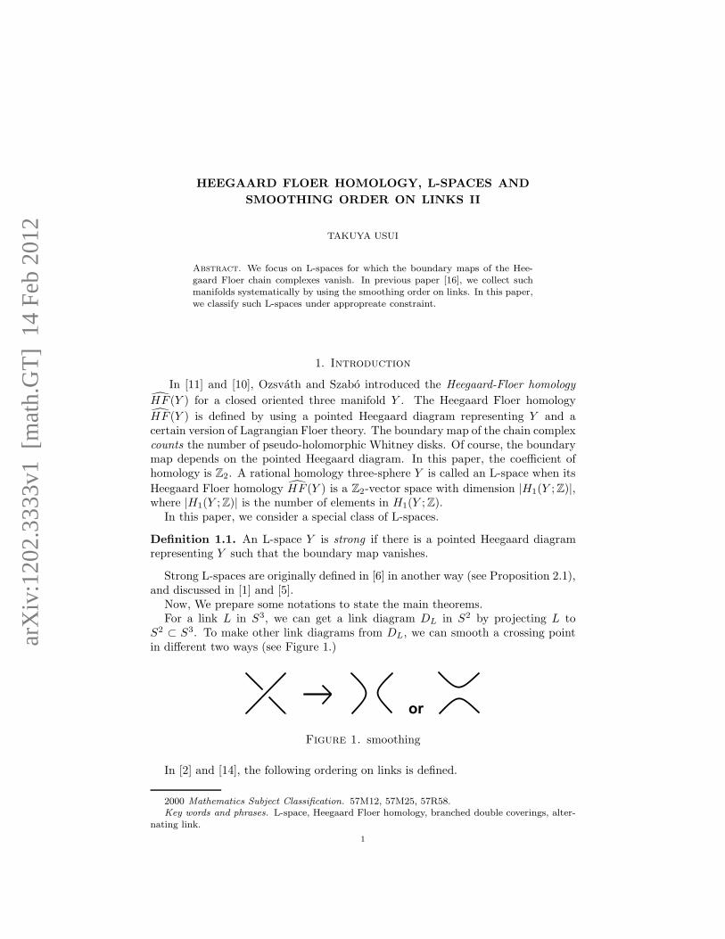
Now, We prepare some notations to state the main theorems.For a link L in S3, we can get a link diagram DL in S2 by projecting L to
S2 ⊂ S3. To make other link diagrams from DL, we can smooth a crossing pointin different two ways (see Figure 1.)
��
Figure 1. smoothing
In [2] and [14], the following ordering on links is defined.
2000 Mathematics Subject Classification. 57M12, 57M25, 57R58.Key words and phrases. L-space, Heegaard Floer homology, branched double coverings, alter-
contains DL1as a connected component after smoothing some
crossing points of DL2.
Let L1 and L2 be alternating links in S3. Then, we say L1 ≤ L2 if for anyminimal crossing alternating link diagram DL2
of L2, there is a minimal crossingalternating link diagram DL1
of L1 such that DL1⊆ DL2
.
These orderings on links and diagrams are called smoothing orders in [2]. Notethat smoothing orders become partial orderings. Let us denote the minimal crossingnumber of L by c(L). If L1 ≤ L2, then c(L1) ≤ c(L2). We can check the well-definedness by using this observation. Actually, if L1 ≤ L2 and L2 ≤ L1, thenc(L1) = c(L2) and there is no smoothed crossing point. So L1 = L2. Next, ifL1 ≤ L2 and L2 ≤ L3, then L1 ≤ L3 by defintion. Note that we can define ≤ forany two links by ignoring alternating conditions. But in this paper we consider onlyalternating links and alternating link diagrams. The Borromean rings Brm are analternating link in S3 whose diagram looks as in Figure 2. We fix this diagram anddenote it by Brm too.
Figure 2. The Borromean rings
Definition 1.3. LBrm = { an alternating link L in S3 such that Brm � L}, whereBrm is the Borromean rings.
Denote Σ(L) a double branched covering of S3 branched along a link L. Thefollowing theorem is proved in [16]:
Theorem 1.1. Let L be a link in S3. If L satisfies the following conditions:
• L ∈ LBrm,• Σ(L) is a rational homology three-sphere,
then Σ(L) is a strong L-space and a graph manifold (or a connected sum of graph-manifolds).
A graph manifold is defined as follows.
Definition 1.4. A closed oriented three manifold Y is a graph manifold if Y canbe decomposed along embedded tori into finitely many Seifert manifolds.
In [16], we also defined the following class of manifolds.
Definition 1.5. (T, σ, w) is an alternatingly weighted tree when the following threeconditions hold.
2
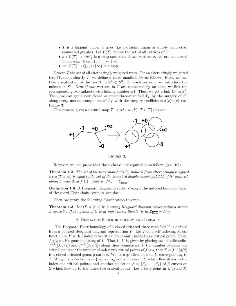
• T is a disjoint union of trees (i.e a disjoint union of simply connected,connected graphs). Let V (T ) denote the set of all vertices of T .
• σ : V (T ) → {±1} is a map such that if two vertices v1, v2 are connectedby an edge, then σ(v1) = −σ(v2).
• w : V (T ) → Q≥0 ∪ {∞} is a map.
Denote T the set of all alternatingly weighted trees. For an alternatingly weightedtree (T, σ, w), shortly T , we define a three manifold YT as follows. First, we cantake a realization of the tree T in R2 ⊂ S3. For each vertex v, we introduce theunknot in S3. Next if two verteces in T are connected by an edge, we link thecorresponding two unknots with linking number ±1. Thus, we get a link LT in S3.Then, we can get a new closed oriented three-manifold YT by the surgery of S3
along every unknot component of LT with the surgery coefficients σ(v)w(v) (seeFigure 3)
This process gives a natural map T → MT = {YT ;T ∈ T }/homeo.
��
��
��
��
�
��
�� ��
�
��
��
Figure 3.
However, we can prove that these classes are equivalent as follows (see [16]).
Theorem 1.2. The set of the three manifolds YT induced from alternatingly weightedtrees (T, σ, w) is equal to the set of the branched double coverings Σ(L) of S3 brancedalong L with Brm � L}. That is, MT = LBrm.
Definition 1.6. A Heegaard diagram is called strong if the induced boundary mapof Heegaard Floer chain complex vanishes.
Then, we prove the following classification theorem.
Theorem 1.3. Let (Σ, α, β, z) be a strong Heegaard diagram representing a strongL-space Y . If the genus of Σ is at most three, then Y is in LBrm = MT .
2. Heegaard-Floer homology and L-spaces
The Heegaard Floer homology of a closed oriented three manifold Y is definedfrom a pointed Heegaard diagram representing Y . Let f be a self-indexing Morsefunction on Y with 1 index zero critical point and 1 index three critical point. Then,f gives a Heegaard splitting of Y . That is, Y is given by glueing two handlebodiesf−1([0, 3/2]) and f−1([3/2, 3]) along their boundaries. If the number of index onecritical points or the number of index two critical points of f is g, then Σ = f−1(3/2)is a closed oriented genus g surface. We fix a gradient flow on Y corresponding tof . We get a collection α = {α1, · · · , αg} of α curves on Σ which flow down to theindex one critical points, and another collection β = {β1, · · · , βg} of β curves onΣ which flow up to the index two critical points. Let z be a point in Σ \ (α ∪ β).
3
The tuple (Σ, α, β, z) is called a pointed Heegaard diagram for Y . Note that α andβ curves are characterized as pairwise disjoint, homologically linearly independent,simple closed curves on Σ. We can assume α-curves intersect β-curves transversaly.
Next, we review the definition of the Heegaard Floer chain complex.Let (Σ, α, β, z) be a pointed Heegaard diagram for Y . The g-fold symmetric
product of the closed oriented surface Σ is defined by Symg(Σ) = Σ×g/Sg. That is,the quotient of Σ×g by the natural action of the symmetric group on g letters.
Let us define Tα = α1 × · · · × αg/Sg and Tβ = β1 × · · · × βg/Sg.
Then, the chain complex CF (Σ, α, β, z) is defined as a free Z2-module generatedby the elements of
where c(x, y) ∈ Z2 is defined by counting the number of pseudo-holomorphic Whit-ney disks. For more details, see [11].
Definition 2.1. [11] The homology of the chain complex (CF (Σ, α, β, z), ∂) iscalled the Heegaard Floer homology of a pointed Heegaard diagram. We denote it
by HF (Σ, α, β, z).
Remark. For appropriate pointed Heegaard diagrams representing Y , their Hee-gaard Floer homologies become isomorphic. So we can define the Heegaard Floer
homology of Y . Denote it by HF (Y ). (For more details, see [11]).
In this paper, we consider only L-spaces, in particular strong L-spaces. Thefollowing proposition enables us to define strong L-spaces in another way. Thesecond condition comes from [6].
Proposition 2.1. Let (Σ, α, β, z) be a pointed Heegaard diagram representing arational homology sphere Y . Then, the following two conditions (1) and (2) areequivalent.
(1) the boundary map ∂ is the zero map, and Y is an L-apace.(2) |Tα ∩ Tβ | = |H1(Y ;Z)|.
For example, any lens-spaces are strong L-spaces. Actually, we can draw a genusone Heegaard diagram representing L(p, q) for which the two circles α and β meettransversely in p points. That is, |Tα ∩ Tβ | = |H1(L(p, q);Z)| = p.
To prove this proposition, we recall that the Heegaard Floer homology HF (Y )admits a relative Z/2Z grading([10]) By using this grading, the Euler characteristicsatisfies the following equation.
χ(HF (Y, s)) = |H1(Y ;Z)|.
Proof. The first condition tells us that CF (Y ) becomes a Z2-vector space with
dimension |H1(Y ;Z)|. By definition of CF (Y ), we get that |Tα ∩Tβ | = |H1(Y ;Z)|.
Conversely, the second condition and the above equation tell us that both CF (Y )
and HF (Y ) become Z2-vector spaces with dimension |H1(Y ;Z)|. Therefore, thefirst condition follows. �
4
3. Strong diagram and induced matrix
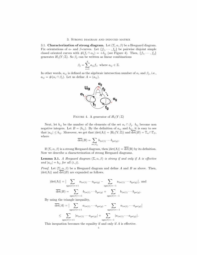
3.1. Characterization of strong diagram. Let (Σ, α, β) be a Heegaard diagram.Fix orientations of α- and β-curves. Let {f1, · · · , fg} be pairwise disjoint simpleclosed oriented curves with #(fi ∩ αj) = +δij (see Figure 4). Then, {f1, · · · , fg}generates H1(Y ;Z). So βj can be written as linear combinations
βj =
g∑
i=1
aijfi, where aij ∈ Z.
In other words, aij is defined as the algebraic intersection number of αi and βj , i.e.,aij = #(αi ∩ βj). Let us define A = (aij).
����
��
��
��
��
��
Figure 4. A generator of H1(Y ;Z)
Next, let bij be the number of the elements of the set αi ∩ βj . bij become nonnegative integers. Let B = (bij). By the definition of aij and bij , it is easy to see
that |aij | ≤ bij . Moreover, we get that |det(A)| = |H1(Y;Z)| and det(B) = Tα∩Tβ ,where
det(B) =∑
σ∈Sg
b1σ(1) · · · bgσ(g).
If (Σ, α, β) is a strong Heegaard diagram, then |det(A)| = det(B) by its definition.Now we describe a characterization of strong Heegaard diagrams.
Lemma 3.1. A Heegaard diagram (Σ, α, β) is strong if and only if A is effectiveand |aij | = bij for all (i, j).
Proof. Let (Σ, α, β) be a Heegaard diagram and define A and B as above. Then,|det(A)| and det(B) are expanded as follows.
|det(A)| =∣∣ ∑
sgn(σ)=+1
a1σ(1) · · · agσ(g) −∑
sgn(σ)=−1
a1σ(1) · · · agσ(g)∣∣, and
det(B) =∑
sgn(σ)=+1
b1σ(1) · · · bgσ(g) +∑
sgn(σ)=−1
b1σ(1) · · · bgσ(g).
By using the triangle inequality,
det(A) =∣∣ ∑
sgn(σ)=+1
a1σ(1) · · · agσ(g) −∑
sgn(σ)=−1
a1σ(1) · · · agσ(g)∣∣
≤∑
sgn(σ)=+1
|a1σ(1) · · · agσ(g)|+∑
sgn(σ)=−1
|a1σ(1) · · · agσ(g)|.
This inequation becomes the equality if and only if A is effective.5
On the other hand, the inequality |aij | ≤ bij implies that
|det(B)| =∑
sgn(σ)=+1
b1σ(1) · · · bgσ(g) +∑
sgn(σ)=−1
b1σ(1) · · · bgσ(g)
≥∑
sgn(σ)=+1
|a1σ(1) · · · agσ(g)|+∑
sgn(σ)=−1
|a1σ(1) · · · agσ(g)|.
This inequation becomes the equality if and only if |aij | = bij for all (i, j).Thus, this lemma follows.
�
Definition 3.1. Let (Σ, α, β) be a strong Heegaard diagram and orient α- and β-curves. The induced matrix A(Σ,α,β) is defined by A(Σ,α,β) = (#(αi ∩ βj))ij .
3.2. Equivalence class of matrices.
Definition 3.2. Let A be a g × g effective matrix. A is not maximal if A can bechanged into a new effective matrix A′ by replacing some 0-component of A with+1 or −1.
Definition 3.3. Let A = (aij) and B = (bij) be g × g matrices. We say A ∼ Bif A can be changed into a new matrix A′ so that each (i, j)-component of A′ hasthe same signature {+,−, 0} as the (i, j)-component of B by some of the followingoperations.
• to permutate two rows or two columns,• to multiple a row or a column by (−1),• to transpose the matrix.
Note that if an effective (or maximal) matrix A is equivalent to B, then B isalso effective (or maximal). Thus, we can define
Eg = {A : effective }/ ∼, and
MEg = {A : maximal and effective }/ ∼⊂ Eg.
Definition 3.4. Let [A] and [B] be two elements of Eg. We say [A] ≤ [B] if wecan change A into A′ by replacing some zero components of A by +1 or −1 so thatthe new class [A′] is equal to [B].
Note that this ordering tells us that an element of MEg is maximal in Eg.For g = 2, we can prove easily that there exists only one maximal effective matrix
A2, i.e., MEg = {[A2]};
A2 =
(+ +− +
),
where we consider only signatures of components of matrices.
Lemma 3.2. For g = 3, there exists only one maximal effective matrix A3, where
A3 =
+ + +− + +0 − +
,
i.e., MEg = {[A3]}
6
Proof. It is easy to see that A3 is a maximal effective matrix. Let A be a maximaleffective 3× 3 matrix. We prove A ∼ A3. First, put
A =
x1 x2 x3
x4 x5 x6
x7 x8 x9
.
Since A is maximal, we can assume that the diagonal components of A are allpositive, i.e., x1 = x5 = x9 = +. We can also assume that there exists at least one0 component, and we can put x7 = 0 (by permutating rows and columns.) Next,we consider the signature of x4.
• If x4 = 0, we can put x6 = + and x8 = − because A is maximal. (bypermutating rows and columns). Then, we can assign arbitrary signaturesto x2 and x3. (A is still effective.) By multipling second or third columnsby (−1), we can assume x2 = x3 = +. This operations may change thesignature of x5, x6,x8 and x9. But by multipling second or third rows by(−1) or permutating rows and columns, we can assume x5 = x6 = x9 = +and x8 = −. Thus, all signatures of A are decided, however A is notmaximal because we can take x4 to be positive. This is contradiction.
A →
+ x2 x3
x4 + x6
0 x8 +
→
+ x2 x3
0 + x6
0 x8 +
→
+ x2 x3
0 + +0 − +
→
+ + +0 + +0 − +
.• If x4 = +, by multipling second row and column by (−1), we can changeso that x4 = −.
• If x4 = −, then x2 = + because A is maximal. If x8 = 0, we can transposeA and we return to the case when x4 = 0. So x8 6= 0. Moreover, we canput x8 = − by multipling third rows and columns by (−1). Lastly, x3 andx6 must be positive because A is maximal. Thus, A ∼ A3.
A →
+ x2 x3
− + x6
0 x8 +
→
+ + x3
− + x6
0 x8 +
→
+ + x3
− + x6
0 − +
→
+ + +− + +0 − +
= A3
.
�
Now we define A′3 as follows.
A′3 =
+ 0 +− + 00 − +
.
Note that [A′3] ≤ [A].
4. In the case g = 2
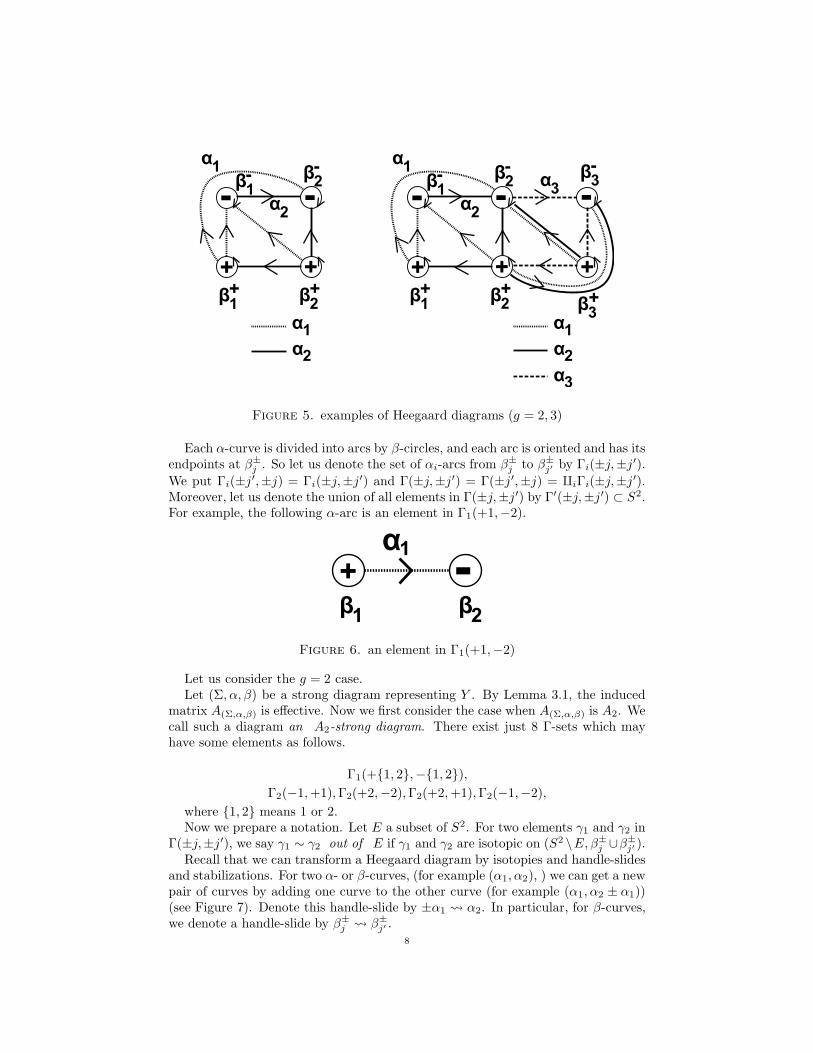
4.1. Types of strong diagrams with g = 2. First, recall that we can describe aHeegaard diagram (Σ, α, β) in R2 as in Figure 5, where 2g signed oriented circlesare β-curves and oriented arcs are α curves. By attaching the corresponding βcircles, we recover the Heegaard diagram (Σ, α, β). Denote each β-circle by β+
j or
β−j .
7
�
� � �
� �
��
�� �
�
��
��
��
� ��
��� �
�� �
��
������
�
� �
�
��
��
��
��
� �
��� �
��
����
Figure 5. examples of Heegaard diagrams (g = 2, 3)
Each α-curve is divided into arcs by β-circles, and each arc is oriented and has itsendpoints at β±
j . So let us denote the set of αi-arcs from β±j to β±
j′ by Γi(±j,±j′).
We put Γi(±j′,±j) = Γi(±j,±j′) and Γ(±j,±j′) = Γ(±j′,±j) = ∐iΓi(±j,±j′).Moreover, let us denote the union of all elements in Γ(±j,±j′) by Γ′(±j,±j′) ⊂ S2.For example, the following α-arc is an element in Γ1(+1,−2).
� ��� ��
��
Figure 6. an element in Γ1(+1,−2)
Let us consider the g = 2 case.Let (Σ, α, β) be a strong diagram representing Y . By Lemma 3.1, the induced
matrix A(Σ,α,β) is effective. Now we first consider the case when A(Σ,α,β) is A2. Wecall such a diagram an A2-strong diagram. There exist just 8 Γ-sets which mayhave some elements as follows.
Γ1(+{1, 2},−{1, 2}),
Γ2(−1,+1),Γ2(+2,−2),Γ2(+2,+1),Γ2(−1,−2),
where {1, 2} means 1 or 2.Now we prepare a notation. Let E a subset of S2. For two elements γ1 and γ2 in
Γ(±j,±j′), we say γ1 ∼ γ2 out of E if γ1 and γ2 are isotopic on (S2 \E, β±j ∪β±
j′ ).Recall that we can transform a Heegaard diagram by isotopies and handle-slides
and stabilizations. For two α- or β-curves, (for example (α1, α2), ) we can get a newpair of curves by adding one curve to the other curve (for example (α1, α2 ± α1))(see Figure 7). Denote this handle-slide by ±α1 α2. In particular, for β-curves,we denote a handle-slide by β±
j β±j′ .
8
�� ��
�� ���
Figure 7. Handle-slide
Proposition 4.1. Let (Σ, α, β) be an A2-strong diagram. Then, (Σ, α, β) can betransformed by handle-slides and isotopies (if it is necessary) so that the new dia-gram is strong and Γ(+j,−j) has at least one element for each j = 1, 2. (However,The new diagram may not be A2-strong.)
Proof. We prove this proposition in two steps.
(1) We can transform (Σ, α, β) so that Γ(+2,−2) 6= ∅.(2) If Γ(+2,−2) 6= ∅, we can transform the diagram so that Γ(+1,−1) 6= ∅
(while keeping the condition Γ(+2,−2) 6= ∅).
In each step, we must take a strong diagram.Step 1 Let (Σ, α, β) be an A2-strong diagram. If Γ(+2,−2) 6= ∅, there is nothing
to do.Suppose that Γ(+2,−2) = ∅. Since #(α2 ∩ β2) 6= 0, we get that Γ(+2,+1) 6= ∅
and Γ(−1,−2) 6= ∅. For any two element γ1 and γ2 in Γ(+2,+1), we get thatγ1 ∼ γ2 out of (β∓
2 ∪β∓1 ∪Γ′(−1,−2)) because S2 \ (β∓
2 ∪β∓1 ∪Γ′(−1,−2)) consists
of disjoint disks. Then, we can transform the diagram by a handle-slide β+2 β+
1 .Note that the new diagram is strong but not A2-strong because Γ2(−1,−2) = ∅.
�
�
�� ��
��
�
��� ��
��
��� ��
���
����
��
Figure 8.
Step 2 Let (Σ, α, β) be anA2-strong diagramwith Γ(+2,−2) 6= ∅. If Γ(+1,−1) 6=∅, there is nothing to do.
Suppose that Γ(+1,−1) = ∅. Since #(α2 ∩ β1) 6= 0, we get that Γ(+2,+1) 6= ∅and Γ(−1,−2) 6= ∅. For any two element γ1 and γ2 in Γ(+2,+1), γ1 ∼ γ2 outof (β∓
2 ∪ β∓1 ∪ Γ′(−1,−2)), because S2 \ (β∓
2 ∪ β∓1 ∪ Γ′(−1,−2) ∪ Γ′(+2,−2)) also
consists of disjoint disks. Then, we can transform the diagram by handle-slidesβ+1 β+
2 finitely many times (see Figure 9). In finitely many steps, we will get9
an A2-strong Heegaard diagram where Γ(+1,−1) 6= ∅. We also get Γ(+2,−2) 6= ∅because the set α1 ∩ β2 becomes non empty after these handle-slides.
�
�
�� ��
��
�
��� ��
�
�
��
���
��� �
��
���
Figure 9.
�
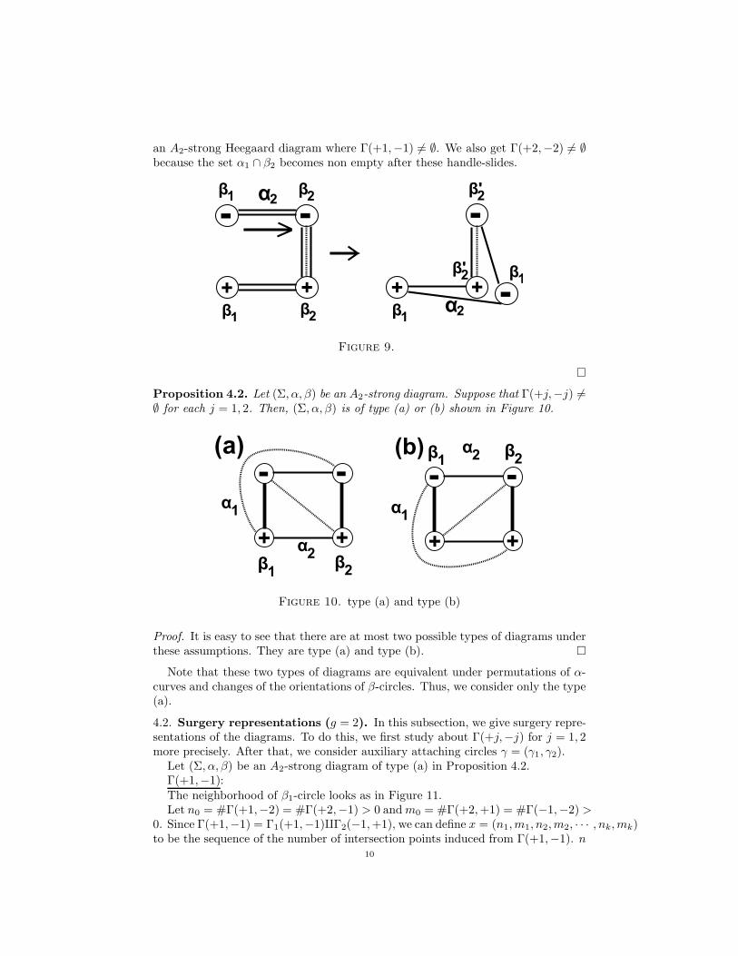
Proposition 4.2. Let (Σ, α, β) be an A2-strong diagram. Suppose that Γ(+j,−j) 6=∅ for each j = 1, 2. Then, (Σ, α, β) is of type (a) or (b) shown in Figure 10.
�
� �
�
��
��
�
� �
���� ��
�
�
�
�
��
��
Figure 10. type (a) and type (b)
Proof. It is easy to see that there are at most two possible types of diagrams underthese assumptions. They are type (a) and type (b). �
Note that these two types of diagrams are equivalent under permutations of α-curves and changes of the orientations of β-circles. Thus, we consider only the type(a).
4.2. Surgery representations (g = 2). In this subsection, we give surgery repre-sentations of the diagrams. To do this, we first study about Γ(+j,−j) for j = 1, 2more precisely. After that, we consider auxiliary attaching circles γ = (γ1, γ2).
Let (Σ, α, β) be an A2-strong diagram of type (a) in Proposition 4.2.Γ(+1,−1):
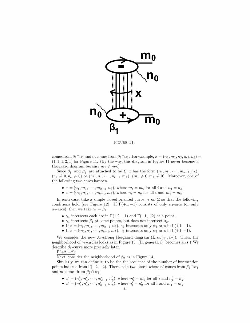
The neighborhood of β1-circle looks as in Figure 11.Let n0 = #Γ(+1,−2) = #Γ(+2,−1) > 0 andm0 = #Γ(+2,+1) = #Γ(−1,−2) >
0. Since Γ(+1,−1) = Γ1(+1,−1)∐Γ2(−1,+1), we can define x = (n1,m1, n2,m2, · · · , nk,mk)to be the sequence of the number of intersection points induced from Γ(+1,−1). n
10
��
��
����
��
�
�
�
Figure 11.
comes from β1∩α1 andm comes from β1∩α2. For example, x = (n1,m1, n2,m2, n3) =(1, 1, 1, 2, 1) for Figure 11. (By the way, this diagram in Figure 11 never become aHeegaard diagram because m1 6= m2.)
Since β+1 and β−
1 are attached to be Σ, x has the form (n1,m1, · · · ,mk−1, nk),(n1 6= 0, nk 6= 0) or (m1, n1, · · · , nk−1,mk), (m1 6= 0,mk 6= 0). Moreover, one ofthe following two cases happen.
• x = (n1,m1, · · · ,mk−1, nk), where mi = m0 for all i and n1 = nk,• x = (m1, n1, · · · , nk−1,mk), where ni = n0 for all i and m1 = mk.
In each case, take a simple closed oriented curve γ1 on Σ so that the followingconditions hold (see Figure 12). If Γ(+1,−1) consists of only α1-arcs (or onlyα2-arcs), then we take γ1 = β1.
• γ1 intersects each arc in Γ(+2,−1) and Γ(−1,−2) at a point.• γ1 intersects β1 at some points, but does not intersect β2.• If x = (n1,m1, · · · ,mk−1, nk), γ1 intersects only α1-arcs in Γ(+1,−1).• If x = (m1, n1, · · · , nk−1,mk), γ1 intersects only α2-arcs in Γ(+1,−1).
We consider the new A2-strong Heegaard diagram (Σ, α, (γ1, β2)). Then, theneighborhood of γ1-circles looks as in Figure 13. (In general, β1 becomes arcs.) Wedescribe β1-curve more precisely later.
Γ(+2,−2):Next, consider the neighborhood of β2 as in Figure 14.Similarly, we can define x′ to be the the sequence of the number of intersection
points induced from Γ(+2,−2). There exist two cases, where n′ comes from β2∩α1
and m comes from β2 ∩ α2.
• x′ = (n′1,m
′1, · · · ,m
′k−1, n
′k), where m′
i = m′0 for all i and n′
1 = n′k,
• x′ = (m′1, n
′1, · · · , n
′k−1,m
′k), where n′
i = n′0 for all i and m′
1 = m′k,
11
Figure 12. γ1-curve
β
+
1
β
+
-
or
γ
γ
-1
1
1
Figure 13. new diagram (Σ, α, (γ1, β2))
�
��
�
�
�
Figure 14.
In each case, take a simple closed oriented curve γ2 on Σ similarly so that thefollowing conditions hold (see Figure 15). If Γ(+2,−2) consists of only α1-arcs (oronly α2-arcs), then we take γ2 = β2.
• γ2 intersects each arc in Γ(+2,−1) and Γ(−1,−2) at a point.12
• γ2 intersects β2 at some points, but does not intersect β1.• If x′ = (n′
1,m′1, · · · ,m
′k−1, n
′k), γ2 intersects only α1-arcs in Γ(+2,−2).
• If x′ = (m′1, n
′1, · · · , n
′k−1,m
′k), γ2 intersects only α2-arcs in Γ(+2,−2).
We consider the new A2-strong Heegaard diagram (Σ, α, γ = (γ1, γ2)). Then,the neighborhood of γ2-circles looks as in Figure 16. (In general, β2 becomes arcs.)
We describe β2-curve more precisely later.
Figure 15. γ2-curve
β
+
2
β
+
-
or
γγ
-2
2
2
Figure 16. new diagram (Σ, α, γ)
Since the new diagram (Σ, α, γ) is easier than the old diagram, we classify theminto four types (see Figure 17). Actually, the new Γ(+j,−j) consists of only α1-arcsor α2-arcs.
But, the type 2-(III) (resp. 2-(IV)) are equivalent to the type 2-(II) (resp. 2-(I))under permutations of α-curves and changes of the orientations of β-curves (beforetaking γ-curves).
type 2-(I) In this case, we get that #Γ(−1,−2) = #Γ(+2,+1) = 1. Thus, we
can take another attaching circles δ = (δ1, δ2) in this diagram such that
• #(δi ∩ γj) = δij for any (i, j) (thus, (Σ, δ, γ) represents S3),• δ1 and δ2 intersects α1 and does not intersect α2.
In this new diagram (Σ, δ, γ), α and β-curves become some framings of someknots in Uδ ∪Uγ . Precisely, we can take three unknots K1, K2 and C1. K1 and K2
are two unknots in Uγ whose framings are β-curves. C1 is an unknot in Uδ whose13
�
� �
�
��
��
�
� �
�
�
� �
�
�
� �
�
����� ������
������� �����
�
�
�
�
��
�
�
�����������
��
��
��
�� �
���
Figure 17. possible types
Figure 18. δ = (δ1, δ2)
framing is α1-curve. Note that α2 can be written by δ-curves as a homology in Σ,so there is no need to consider. These slopes can be determined as follows.
Let rα1, rβ1
and rβ2be the rational numbers representing the surgery framings
of α1, β1 and β2 respectively. Precisely, these rational numbers are determined asfollows. Put rα1
= sgn(rα1)p1/q1 and rβi
= sgn(rβi)p′i/q
′i for i = 1, 2. Then,
• sgn(rα1) = sgn(rβ1
) = sgn(rβ2) = +1,
• p1 = #(α1 ∩ (γ1 ∪ γ2),• q1 = #(Γ(+1,−2)),• p′i = #(βi ∩ α2), for i = 1, 2.• q′i = #(βi ∩ γi), for i = 1, 2.
14
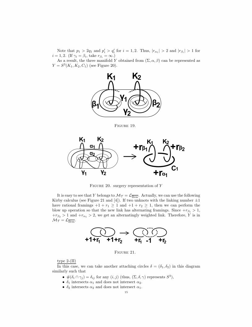
Note that p1 > 2q1 and p′i > q′i for i = 1, 2. Thus, |rα1| > 2 and |rβi
| > 1 fori = 1, 2. (If γi = βi, take rβi
= ∞.)As a result, the three manifold Y obtained from (Σ, α, β) can be represented as
Y = S3(K1,K2, C1) (see Figure 20).
γ1 β2γ2
β1
K1 K2
Figure 19.
γ1
α2
γ2
α1
K1 K2 K1 K2+rβ1 +rβ2
+rα1C1
Figure 20. surgery representation of Y
It is easy to see that Y belongs toMT = LBrm. Actually, we can use the followingKirby calculus (see Figure 21 and [4]). If two unknots with the linking number ±1have rational framings +1 + r1 ≥ 1 and +1 + r2 ≥ 1, then we can perform theblow up operation so that the new link has alternating framings. Since +rβ1
> 1,+rβ2
> 1 and +rα1> 2, we get an alternatingly weighted link. Therefore, Y is in
MT = LBrm.
����� ����� ��� �� ���
Figure 21.
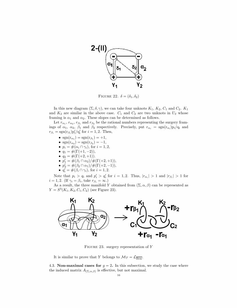
type 2-(II)
In this case, we can take another attaching circles δ = (δ1, δ2) in this diagramsimilarly such that
• #(δi ∩ γj) = δij for any (i, j) (thus, (Σ, δ, γ) represents S3),• δ1 intersects α1 and does not intersect α2.• δ2 intersects α2 and does not intersect α1.
15
Figure 22. δ = (δ1, δ2)
In this new diagram (Σ, δ, γ), we can take four unknots K1, K2, C1 and C2. K1
and K2 are similar in the above case. C1 and C2 are two unknots in Uδ whoseframing is α1 and α2. These slopes can be determined as follows.
Let rα1, rα2
, rβ1and rβ2
be the rational numbers representing the surgery fram-ings of α1, α2, β1 and β2 respectively. Precisely, put rαi
= sgn(rαi)pi/qi and
rβi= sgn(rβi
)p′i/q′i for i = 1, 2. Then,
• sgn(rα1) = sgn(rβ1
) = +1,• sgn(rα2
) = sgn(rβ2) = −1,
• pi = #(αi ∩ γi), for i = 1, 2,• q1 = #(Γ(+1,−2)),• q2 = #(Γ(+2,+1)).• p′1 = #(β1 ∩ α2)/#(Γ(+2,+1)),• p′2 = #(β2 ∩ α1)/#(Γ(+2,−1)),• q′i = #(βi ∩ γi), for i = 1, 2.
Note that pi > qi and p′i > q′i for i = 1, 2. Thus, |rαi| > 1 and |rβi
| > 1 fori = 1, 2. (If γi = βi, take rβi
= ∞.)As a result, the three manifold Y obtained from (Σ, α, β) can be represented as
Y = S3(K1,K2, C1, C2) (see Figure 23).
γ1
α2
γ2
α1
K1 K2 K1 K2+rβ1 -rβ2
+rα1
C1 C2
-rα1Figure 23. surgery representation of Y
It is similar to prove that Y belongs to MT = LBrm.
4.3. Non-maximal cases for g = 2. In this subsection, we study the case wherethe induced matrix A(Σ,α,β) is effective, but not maximal.
16
Let (Σ, α, β) be a strong diagram with genus two. If the induced matrix is notA2, then
A(Σ,α,β) ∼
(+ 00 +
)or
(+ +0 +
).
The first matrix implies that Y becomes a connected sum of Lens space. If A(Σ,α,β)
is the second matrix, we find that Γ(+2,−2) 6= ∅, Γ(+1,−2) 6= ∅ and Γ(+2,−1) 6= ∅.So the neighborhood of β2 looks as in Figure 24. Let x = (n1,m1, · · · ,mk−1, nk)be the sequence of integers representing Γ(+2,−2), where n means β2 ∩ α1 and mmeans β2 ∩ α2. Note that x can not be of the form (m1, n1, · · · , nk−1,mk). SinceΓ(+2,+1) = ∅, we find that ni = 1 for all i. Thus, we can transform the diagramby handle-slides α1 α2 (see Figure 24).
This new diagram implies that Y is a connected sum of lens spaces.
��
�
� ��
�
�
Figure 24. not maximal case
5. Proof of Theorem 1.3
5.1. Types of A′3-strong diagrams for g = 3. Let (Σ, α, β) be a strong diagram
representing Y with genus three. Suppose that the equivalence class of the inducedmatrix satisfies [A′
3] ≤ [A(Σ,α,β)]. We call such a diagram an A′3-strong diagram.
Recall that [A′3] ≤ [A3]. There are just 22 Γ-sets which may have some elements as
Proposition 5.1. Let (Σ, α, β) be an A′3-strong diagram. Then, (Σ, α, β) can be
transformed by handle-slides and isotopies (if it is necessary) so that the new dia-gram is strong and Γ(+j,−j) has at least one element for each j = 1, 2, 3.
Proof. We prove this proposition in three steps. Compare this proof with the proofof Proposition 4.1.
(1) We can transform the diagram so that Γ(+3,−3) 6= ∅.(2) If Γ(+3,−3) 6= ∅, we can transform the diagram so that Γ(+2,−2) 6= ∅.(3) If Γ(+3,−3) 6= ∅ and Γ(+2,−2) 6= ∅, we can transform the diagram so that
Γ(+1,−1) 6= ∅.17
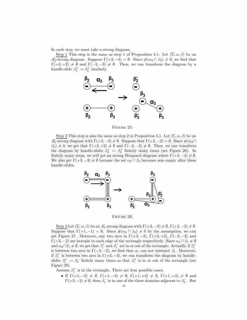
In each step, we must take a strong diagram.Step 1 This step is the same as step 1 of Proposition 4.1. Let (Σ, α, β) be an
A′3-strong diagram. Suppose Γ(+3,−3) = ∅. Since #(α3 ∩ β3) 6= 0, we find that
Γ(+3,+2) 6= ∅ and Γ(−2,−3) 6= ∅. Then, we can transform the diagram by ahandle-slide β+
3 β+2 similarly.
�
�
��
��
��
�
��� ��
��
��� ��
���
����
��
Figure 25.
Step 2 This step is also the same as step 2 in Proposition 4.1. Let (Σ, α, β) be an
A′3-strong diagram with Γ(+3,−3) 6= ∅. Suppose that Γ(+2,−2) = ∅. Since #(α3∩
β2) 6= 0, we get that Γ(+3,+2) 6= ∅ and Γ(−2,−3) 6= ∅. Then, we can transformthe diagram by handle-slides β+
2 β+3 finitely many times (see Figure 26). In
finitely many steps, we will get an strong Heegaard diagram where Γ(+2,−2) 6= ∅.We also get Γ(+3,−3) 6= ∅ because the set α2 ∩ β3 becomes non empty after thesehandle-slides.
�
�
��
��
��
�
��� ��
�
�
���
��
��� �
���
��
Figure 26.
Step 3 Let (Σ, α, β) be anA′3-strong diagramwith Γ(+3,−3) 6= ∅, Γ(+2,−2) 6= ∅.
Suppose that Γ(+1,−1) = ∅. Since #(α3 ∩ β2) 6= 0 by the assumption, we canget Figure 27. Moreover, any two arcs in Γ(+3,−3), Γ(+3,+2), Γ(−3,−2) andΓ(+2,−2) are isotopic to each edge of the rectangle respectively. Since α1 ∩β1 6= ∅and α2∩β1 6= ∅, we get that β+
1 and β−1 are in or out of the rectangle. Actually, if β+
1
is between two arcs in Γ(−3,−2), we find that α1 can not intersect β1. Moreover,if β+
1 is between two arcs in Γ(+3,−3), we can transform the diagram by handle-slides β+
1 β−3 finitely many times so that β+
1 is in or out of the rectangle (seeFigure 28).
Assume β+1 is in the rectangle. There are four possible cases.
• If Γ(+1,−2) 6= ∅, Γ(+1,−3) 6= ∅, Γ(+1,+2) 6= ∅, Γ(+1,+3) 6= ∅ andΓ(+3,−2) 6= ∅, then β−
1 is in one of the three domains adjacent to β−3 . But
18
�
�
��
��
��
�
�
Figure 27. Γ(+3,−3), Γ(+3,+2), Γ(−3,−2) and Γ(+2,−2)make a rectangle
�
�
��
��
�
����
�
�
����
�
����
�
�
�� ��
�
�� ��
�
�
�� ��
�
� ���
Figure 28. positions of β+1
one of them is impossible because Γ(+2,−1) 6= ∅ (see Figure 29). In theother two cases, we can transform the diagram by handle-slides β−
1 β−3
finitely many times. Thus, we get Γ(+1,−1) 6= ∅. Of course, the diagramis strong and Γ(+3,−3) 6= ∅ and Γ(+2,−2) 6= ∅.
• If Γ(+1,−2) 6= ∅, Γ(+1,−3) 6= ∅, Γ(+1,+2) 6= ∅, Γ(+1,+3) 6= ∅ andΓ(−3,+2) 6= ∅, we can get Γ(+1,−1) 6= ∅ similarly.
• If Γ(+1,−2) 6= ∅, Γ(+1,−3) 6= ∅, Γ(+1,+2) 6= ∅, Γ(+1,+3) 6= ∅, Γ(+3,−2) =∅ and Γ(−3,+2) = ∅, then β−
1 is in one of the following two domains as in19
�
�
��
��
�
�
���
�� �
������ �
Figure 29.
Figure 30 because #(α1 ∩ β+3 ) = #(α1 ∩ β−
3 ). Thus, we can also transformthe diagram by handle-slides β−
1 β−3 finitely many times so that we get
Γ(+1,−1) 6= ∅.
�
�
�� ��
�
�
���
� �
Figure 30.
• If one of Γ(+1,−2), Γ(+1,−3), Γ(+1,+2), Γ(+1,+3) is the empty set, thenwe can transform the diagram by handle-slides finitely many times so thatwe get Γ(+1,−1) 6= ∅ as follows.
– Γ(+1,+3) = ∅ ⇒ β+1 β+
2 .– Γ(+1,−3) = ∅ ⇒ β+
1 β−2 .
– Γ(+1,+2) = ∅ ⇒ β+1 β+
3 .– Γ(+1,−2) = ∅ ⇒ β+
1 β−3 .
�
Proposition 5.2. Let (Σ, α, β) be an A′3-strong diagram. Suppose Γ(+j,−j) 6=
∅ for j = 1, 2, 3. Then, (Σ, α, β) can be transformed by handle-slides, isotopies,permutations of curves, changes of orientations(if it is necessary) so that the newstrong diagram is of one of the following three types 3-(a), 3-(b) and 3-(c) (seeFigure 31).
Proof. By Proposition 5.1, we can assume Γ(+j,−j) 6= ∅ for all j. We put β1 andβ2 as in Figure . Then, β3 is in one of the three domains as in Figure .
• The position (i) is impossible because Γ(+3,+2) 6= ∅.20
�
� � �
� �
���
�
� � �
� �
���
�
� � �
� �
����
Figure 31. three possoble types
�
�
���
�
�
�
�
�
���
�
�
�
� ��� � ���� ����
�����
Figure 32. three positions
• If β3 is in (ii), β1 and β2 looks as in Figure 33. Since Γ(+1,−2) 6=∅ and Γ(−1,−2) 6= ∅, we can transform the diagram by handle-slides(β+
1 and β−1 ) β−
2 finitely many times so that the new diagram is alsoA′
3-strong and β3 is in the position (iii).
�
�
��
����
�
�
��
�
�
��
�� ��
�
�
��
Figure 33.
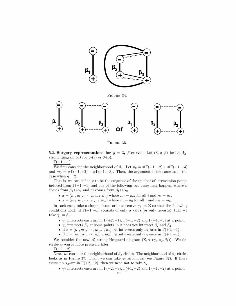
• If β3 is in (iii), there exist at most two isotopy classes of arcs in Γ(+3,−3)(see 34). If there exist two arcs which are not isotopic, then we can trans-form the diagram by handle-slides (β+
2 and β−2 ) β−
3 finitely many timesso that all arcs in Γ(+j,−j) are isotopic (see Figure 34).
Since Γ(+3,+2) 6= ∅ and Γ(−3,−2) 6= ∅, we get two possible cases as in Figure 35.But they are equivalent under permutating β2 and β3 and reversing the orientationof α3.
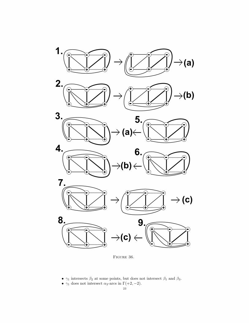
Now we can describe all possible cases. There are another 9 cases, but we cantransform these diagrams into one of the three types. �
However, note that the type (c) never happens. Actually, the pattern of theintersection points at β+
3 and β−3 never coincide, so we can not attach β3-circles.
21
�
�
��
�
�
��
�
�
��
Figure 34.
�
�
��
�
�
��
�
�
��
�
�
��
�
�
��
�
�
����
Figure 35.
5.2. Surgery representations for g = 3, β-curves. Let (Σ, α, β) be an A′3-
strong diagram of type 3-(a) or 3-(b).Γ(+1,−1):
We first consider the neighborhood of β1. Let n0 = #Γ(+1,−2) + #Γ(+1,−3)and m0 = #Γ(+1,+2) + #Γ(+1,+3). Then, the argument is the same as in thecase when g = 2.
That is, we can define x to be the sequence of the number of intersection pointsinduced from Γ(+1,−1) and one of the following two cases may happen, where ncomes from β1 ∩ α1 and m comes from β1 ∩ α2.
• x = (n1,m1, · · · ,mk−1, nk) where mi = m0 for all i and n1 = nk,• x = (m1, n1, · · · , nk−1,mk) where ni = n0 for all i and m1 = mk.
In each case, take a simple closed oriented curve γ1 on Σ so that the followingconditions hold. If Γ(+1,−1) consists of only α1-arcs (or only α2-arcs), then wetake γ1 = β1.
• γ1 intersects each arc in Γ(+2,−1), Γ(−1,−2) and Γ(−1,−3) at a point.• γ1 intersects β1 at some points, but does not intersect β2 and β3.• If x = (n1,m1, · · · ,mk−1, nk), γ1 intersects only α1-arcs in Γ(+1,−1).• If x = (m1, n1, · · · , nk−1,mk), γ1 intersects only α2-arcs in Γ(+1,−1).
We consider the new A′3-strong Heegaard diagram (Σ, α, (γ1, β2, β3)). We de-
scribe β1-curve more precisely later.Γ(+2,−2):Next, we consider the neighborhood of β2-circles. The neighborhood of β2-circles
looks as in Figure 37. Then, we can take γ2 as follows (see Figure 37). If thereexists no α3-arc in Γ(+2,−2), then we need not to take γ2.
• γ2 intersects each arc in Γ(−2,−3), Γ(+1,−2) and Γ(−1,−2) at a point.22
�
� � �
� �
� � �
� ��
���
� � �
� �
��
��
��
�
�
� �
� �
�
�
� �
� �
�
� � �
� �
� � �
� ��
����
�
�
� �
� �
��
�
��
��
�
��
�
�
� �
� �
�
�
� �
� �
�
� � �
� �
� � �
� ��
���
���
�� ��
Figure 36.
• γ1 intersects β2 at some points, but does not intersect β1 and β3.• γ1 does not intersect α3-arcs in Γ(+2,−2).
23
We consider the new A′3-strong Heegaard diagram (Σ, α, (γ1, γ2, β3)). Then,
the neighborhood of γ2-circles looks as in Figure 37. We describe β2-curve moreprecisely later.
β+
-
2 β+
-
2
Figure 37. γ2-curve and new diagram (Σ, α, (γ1, γ2, β3))
Γ(+3,−3): Lastly, consider the neighborhood of β3 looks as in Figure 38.
�
��
�
�
�Figure 38.
Similarly, we can define x′ to be the the sequence of the number of intersectionpoints induced from Γ(+3,−3). In this case, it is convinient not to distinguish α1
and α3. That is, there exist two cases, where n′ comes from β3 ∩ α3 and m comesfrom β3 ∩ (α1 ∪ α2).
• x′ = (n′1,m
′1, · · · ,m
′k−1, n
′k) where m′
i = m′0 for all i and n′
1 = n′k,
• x′ = (m′1, n
′1, · · · , n
′k−1,m
′k) where n′
i = n′0 for all i and m′
1 = m′k.
Moreover, if x′ = (m′1, n
′1, · · · , n
′k−1,m
′k), we find that n′
i = 1 for all i. Otherwise,α3-arcs can not be a closed curve. Then, We can transform the diagram by m′
1
handle-slides +(α1 and α2) α3 (see Figure 39) so that the new diagram is also24
A′3-strong diagram and Γi(+3,−3) = ∅ for i = 1, 2. As a result, we return to the
first case.
��
�
�
��
��
�
�
��
Figure 39.
If x′ = (n′1,m
′1, · · · ,m
′k−1, n
′k), take a simple closed oriented curve γ3 on Σ
similarly so that the following conditions hold (see Figure 40). If Γ(+3,−3) consistsof only α3-arcs, then we take γ3 = β3.
• γ3 intersects each arc in Γ(−2,−3), Γ(+1,−3) and Γ(+2,−3)at a point.• γ3 intersects β3 at some points, but does not intersect β1 and β2.• γ3 intersects only α3-arcs in Γ(+2,−2).
We consider the new A′3-strong Heegaard diagram (Σ, α, γ = (γ1, γ2, γ3)). Then,
the neighborhood of γ2-circles looks as in Figure 40. (In general, β2 becomes arcs.)We describe β3-curve more precisely later.
β+
-
3
+
-γ3
γ3
Figure 40. γ3 and new diagram (Σ, α, γ)
Thus, there exist four possible types (see Figure 41).In each case, βj-curves become some surgery framings of some unknots K1, K2
and K3 by attaching γj-circles (see Figure 42).
5.3. Surgery representations for g = 3, α-curves. Now, we recall positive (ornegative) Dehn twists.
Definition 5.1. Let Σ be a closed oriented genus g surface and Let c1 be asimple closed curve on Σ. Then, a positive (or negative) Dehn twist is the self-homeomorphism ±f(c1) on Σ defined as in Figure 43-(p) and (n) on a neighbor-hood of c1, where a curve c2 is mapped to f(c2) by f . On the other hand, ±f(c1)is identity on Σ \ nbd(c1).
25
�
� � �
� �
�� � �
�
� � �
� �
�
� � �
� �
�
� � �
� �
���� �����
������ ����
�� �
�
��
��
��
��
� �
Figure 41. possible four types
γ1 β2γ2
β1
K1 K2
�
K�
γ
Figure 42.
�
�������
��
�
�
�
������
�
�
�� ���
Figure 43. positive/negative Dehm surgery
Let (Σ, α, β) be an A′3-strong diagram of type 3-(I), 3-(II), 3-(III) or 3-(IV). Let
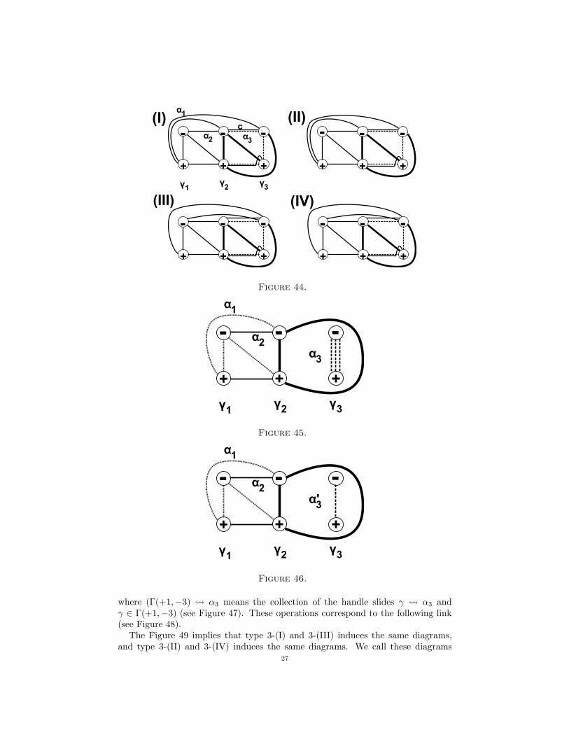
c be a simple closed curve on Σ which intersects Γ(+2,+3), Γ(+3,−2), γ2 and γ3 asin Figure 44. We perform a positive Dehn twist along c. Then, α-arcs are changedas in Figure 45. Note that γ3 intersects only α3. Thus, α3-curves become a surgeryframing of a unknot C3 in Uα. We describe the slope precisely later. Let α′
3 be thesimple closed curve which intersects only γ3 at one point (see Figure 46).
Next, we consider the simple closed curve c as above again. We perform a nega-tive Dehn twist along c (see Figure 44). Since α′
3 still intersects γ3 at only one point,we can transform the diagram by a handle-slide (Γ(+1,−3) and Γ(+2,−3)) α3,
26
-
+ + +
- -
γ1 2 3
-
+ + +
- -
-
+ + +
- -
-
+ + +
- -
(I) (II)
(III) (IV)
α1
α2 α3
c
γ γ
Figure 44.
�
� � �
� �
��
��
��
��
��
��
Figure 45.
�
� � �
� �
��
��
��
��
��
���
Figure 46.
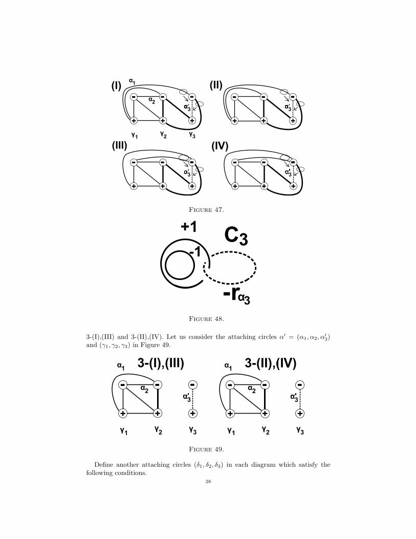
where (Γ(+1,−3) α3 means the collection of the handle slides γ α3 andγ ∈ Γ(+1,−3) (see Figure 47). These operations correspond to the following link(see Figure 48).
The Figure 49 implies that type 3-(I) and 3-(III) induces the same diagrams,and type 3-(II) and 3-(IV) induces the same diagrams. We call these diagrams
27
�
� � �
� �
�� � �
�
� � �
� �
�
� � �
� �
�
� � �
� �
�� ���
���� ��
��
��
���
� �
����
����
���
Figure 47.
��
����
��
��
Figure 48.
3-(I),(III) and 3-(II),(IV). Let us consider the attaching circles α′ = (α1, α2, α′3)
and (γ1, γ2, γ3) in Figure 49.
�
� � �
� �
�� � �
���� ������
��
���
� �
�
� � �
� �
�� � �
����� � ��
��
��
� �
Figure 49.
Define another attaching circles (δ1, δ2, δ3) in each diagram which satisfy thefollowing conditions.
28
• #(δi ∩ γj) = δij for any (i, j) (thus, (Σ, δ, γ) represents S3),• If in the case of 3-(I),(III), δ1 intersects α1 and does not intersect α2.• If in the case of 3-(II),(IV), δ1 intersects α2 and does not intersect α1.• δ2 intersects α-curves atN points, whereN < #(Γ(+2,−2))+#(Γ(+2,−1))+#(Γ(+2,+1)).
• δ3 = α′3
Let us denote D1 and D3 be properly embedded disks in Uδ such that ∂D1 = δ1and ∂D3 = δ3. If we cut the handlebody Uδ along D1 and D3, then Uδ \ (D1 ∪D3)becomes a solid torus. Let us denote the core of the solid torus by C2. Then,
• α2 becomes the surgery framing of C2 in the case of 3-(I),(III), and• α1 becomes the surgery framing of C2 in the case of 3-(II),(IV).
On the other hand, it is easy to see that there exists a C1 in Uδ such that
• α1 become the surgery framings of C1 in the case of 3-(I),(III), and• α2 become the surgery framings of C1 in the case of 3-(II),(IV).
Note that C1 becomes a torus knot in S3 in genaral. We describe these slopes later.As a result, a Heegaard diagrams of each type is represented by a surgery of
S3 along some link (see Figure 50 and 51). Let us denote the framed link inducedfrom 3-(I),(III) by L(13) and the framed link induced from 3-(II),(IV) by L(24).Moreover, let us denote the manifolds induced from these links L(13) and L(24) byM(13) and M(24). Now we denote the framing of these links shortly. Let rαi
bethe framing of Cj corresponding to αi for any (i, j). Let rβj
be the framing of Kj
corresponding to βj for any j.
��
��
����
��
��
��
���� ��
�� ��
��
���
��
Figure 50. 3-(I),(III)
��
�
����
��
��
��
����
��
����
��
�� �
��
Figure 51. 3-(II),(IV)
29
5.4. Determination of manifolds for g = 3. In this subsection, we finish toprove Theorem 1.3. Recall there are two cases to be considered.
3-(I),(III) Let (Σ, α, β) be an A′3-strong diagram of type 3-(I),(III) (see Figure
49). Recall that rαiis the framing of Ci corresponding to αi for any i, and rβj
isthe framing of Kj corresponding to βj for any j.
Then, C1 becomes the (p2, q2)-torus knot and it is linking with C2, where theframing of the (p2, q2)-torus becomes the integer p2 + q2 − 1. We also find that, byeasy obsevations,
• +p1/q1 > +1,• rα2
> +1,• rβ1
> +1,• rβ2
< −1,• rβ3
< −1.
Next, we describe the relation between p2/q2 and p′2/q′2 precisely. We can rep-
resent p2/q2 as the continuous fraction expansion as follows.
(2)p2q2
= k1 +1
k2 +1
· · ·+1
kn−1 +1
kn
, where ki ≥ 1 and kn ≥ 2.
By using these integers, we put a new rational number R(p2, q2, p′2, q
′2) as follows.
(3) R(p2, q2, p′2, q
′2) = −(kn +
1
kn−1 +1
· · ·+1
k2 +1
k1 −p′2q′2
).
Then, we can prove the following claim.30
Claim 5.1. Let p2/q2, p′2/q
′2) and R(p2, q2, p
′2, q
′2) be the rational numbers defined
as above. Then, we get that
• R(p2, q2, p′2, q
′2) > 0 if n is odd, and
• −1 < R(p2, q2, p′2, q
′2) < 0 if n is even.
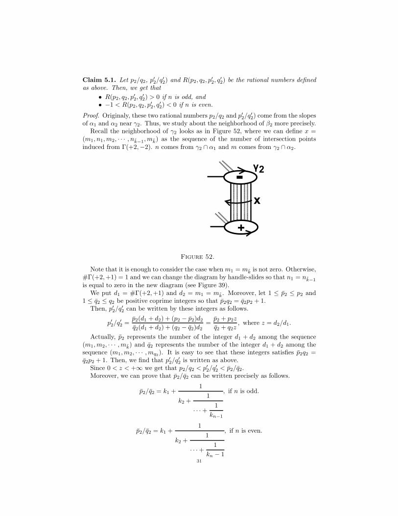
Proof. Originaly, these two rational numbers p2/q2 and p′2/q′2) come from the slopes
of α1 and α2 near γ2. Thus, we study about the neighborhood of β2 more precisely.Recall the neighborhood of γ2 looks as in Figure 52, where we can define x =
(m1, n1,m2, · · · , nk−1,mk) as the sequence of the number of intersection pointsinduced from Γ(+2,−2). n comes from γ2 ∩ α1 and m comes from γ2 ∩ α2.
�
���
�
Figure 52.
Note that it is enough to consider the case when m1 = mk is not zero. Otherwise,#Γ(+2,+1) = 1 and we can change the diagram by handle-slides so that n1 = nk−1
is equal to zero in the new diagram (see Figure 39).We put d1 = #Γ(+2,+1) and d2 = m1 = mk. Moreover, let 1 ≤ p2 ≤ p2 and
1 ≤ q2 ≤ q2 be positive coprime integers so that p2q2 = q2p2 + 1.Then, p′2/q
Actually, p2 represents the number of the integer d1 + d2 among the sequence(m1,m2, · · · ,mk) and q2 represents the number of the integer d1 + d2 among thesequence (m1,m2, · · · ,mq2). It is easy to see that these integers satisfies p2q2 =q2p2 + 1. Then, we find that p′2/q
′2 is written as above.
Since 0 < z < +∞ we get that p2/q2 < p′2/q′2 < p2/q2.
Moreover, we can prove that p2/q2 can be written precisely as follows.
p2/q2 = k1 +1
k2 +1
· · ·+1
kn−1
, if n is odd.
p2/q2 = k1 +1
k2 +1
· · ·+1
kn − 1
, if n is even.
31
This equation comes from the Euclidean algorithm. Thus, we also find that thelength of the continuous fraction expansion of p′2/q
′2 is n or grater than n. In
particular, R(p2, q2, p′2, q
′2) is well-defined.
Finally, we conclude that
R(p2, q2, p′2, q
′2) = −(kn +
1
kn−1 +1
· · ·+1
k2 +1
k1 − p′2/q′2
) > 0,
if n is odd, and
0 > R(p2, q2, p′2, q
′2) > −(kn +
1
kn−1 +1
· · ·+1
k2 +1
k1 − p2/q2
) = −1,
if n is even. �
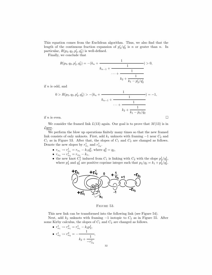
We consider the framed link L(13) again. Our goal is to prove that M(13) is inLBrm.
We perform the blow up operations finitely many times so that the new framedlink consists of only unknots. First, add k1 unknots with framing −1 near C2 andC1 as in Figure 53. After that, the slopes of C1 and C2 are changed as follows.Denote the new slopes by r1α1
and r1α2.
• rα1 r1α1
= rα1− k1q
02 , where q02 = q2,
• rα2 r1α2
= rα2− k1,
• the new knot C11 induced from C1 is linking with C2 with the slope p12/q
12,
where p12 and q12 are positive coprime integer such that p2/q2 = k1 + p12/q12.
��
���
����
��
��
��
��
����
��
��
�
�
����
�
��
��
Figure 53.
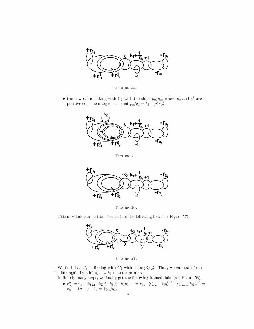
This new link can be transformed into the following link (see Figure 54).Next, add k2 unknots with framing −1 isotopic to C2 as in Figure 55. After
some Kirby calculus, the slopes of C1 and C2 are changed as follows.
• r1α1 r2α1
= r1α1− k2p
12,
• r1α2 r2α2
= −1
k2 +1
−r1α2
,
32
�
��
��
��
��
����
��
��
���
�
��
�
��
��
�
Figure 54.
• the new C21 is linking with C2 with the slope p22/q
22 , where p22 and q22 are
positive coprime integer such that p12/q12 = k2 + p22/q
22.
�
��
��
��
��
����
��� �
��
���
�
��
�
��
��
�
��
Figure 55.
��
��
��
��
����
��
��
���
��
���
�
��
��
��
���
Figure 56.
This new link can be transformed into the following link (see Figure 57).
��
��
��
��
����
��
��
���
��
���
�
��
��
��
����
�
Figure 57.
We find that C21 is linking with C2 with slope p22/q
22 . Thus, we can transform
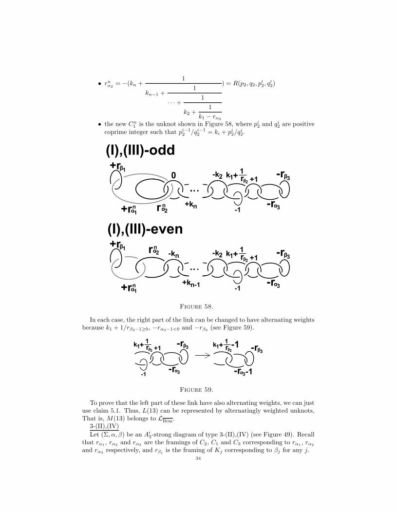
this link again by adding new k3 unknots as above.In finitely many steps, we finally get the following framed links (see Figure 58).
• rnα1= rα1
−k1q2−k2p12−k3q
22−k4p
32 · · · = rα1
−∑
i:odd kiqi−12 −
∑i:even kip
i−12 =
rα1− (p+ q − 1) = +p1/q1,
33
• rnα2= −(kn +
1
kn−1 +1
· · ·+1
k2 +1
k1 − rα2
) = R(p2, q2, p′2, q
′2)
• the new Cn1 is the unknot shown in Figure 58, where pi2 and qi2 are positive
coprime integer such that pi−12 /qi−1
2 = ki + pi2/qi2.
��
��
�
��
����
��
��
���
�
��
�
�� ��
�
��
���
�
��
�����
��
�� ���
�
���
�
��
�
�� ��
�
��
����
��
� ��� ����
� ��� �����
Figure 58.
In each case, the right part of the link can be changed to have alternating weightsbecause k1 + 1/rβ2−1≥0, −rα3−1<0 and −rβ3
(see Figure 59).
�� ���
��
����
��
�
�
��
�� ���
��
����
��
�
��
��
Figure 59.
To prove that the left part of these link have also alternating weights, we can justuse claim 5.1. Thus, L(13) can be represented by alternatingly weighted unknots,That is, M(13) belongs to LBrm.
3-(II),(IV)
Let (Σ, α, β) be an A′3-strong diagram of type 3-(II),(IV) (see Figure 49). Recall
that rα1, rα2
and rα3are the framings of C2, C1 and C3 corresponding to rα1
, rα2
and rα3respectively, and rβj
is the framing of Kj corresponding to βj for any j.34
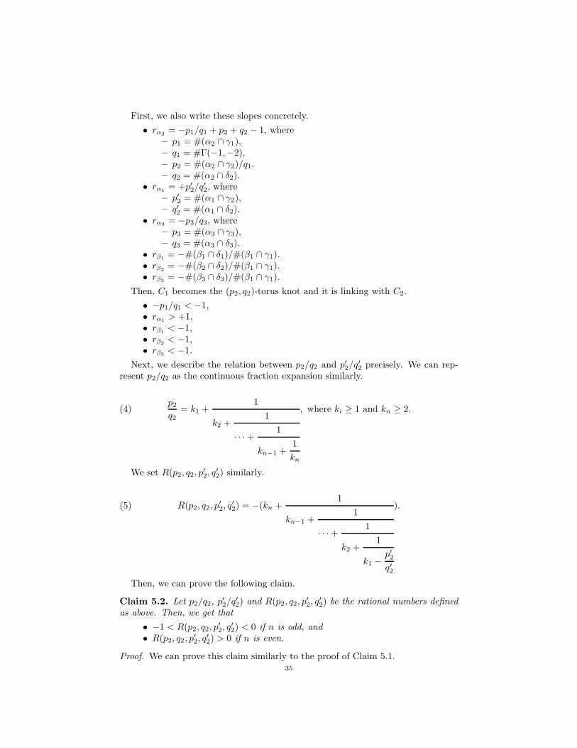
Then, C1 becomes the (p2, q2)-torus knot and it is linking with C2.
• −p1/q1 < −1,• rα1
> +1,• rβ1
< −1,• rβ2
< −1,• rβ3
< −1.
Next, we describe the relation between p2/q2 and p′2/q′2 precisely. We can rep-
resent p2/q2 as the continuous fraction expansion similarly.
(4)p2q2
= k1 +1
k2 +1
· · ·+1
kn−1 +1
kn
, where ki ≥ 1 and kn ≥ 2.
We set R(p2, q2, p′2, q
′2) similarly.
(5) R(p2, q2, p′2, q
′2) = −(kn +
1
kn−1 +1
· · ·+1
k2 +1
k1 −p′2q′2
).
Then, we can prove the following claim.
Claim 5.2. Let p2/q2, p′2/q
′2) and R(p2, q2, p
′2, q
′2) be the rational numbers defined
as above. Then, we get that
• −1 < R(p2, q2, p′2, q
′2) < 0 if n is odd, and
• R(p2, q2, p′2, q
′2) > 0 if n is even.
Proof. We can prove this claim similarly to the proof of Claim 5.1.35
Actually, if we define x = (n1,m1, n2, · · · ,mk−1, nk) as the sequence of thenumber of intersection points induced from Γ(+2,−2), then we can assume n1 = nk
is not zero.Let d1 = #Γ(+2,−1) and d2 = n1 = nk. We take positive coprime integers
1 ≤ p2 ≤ p2 and 1 ≤ q2 ≤ q2 so that p2q2 = q2p2 − 1.Then, p′2/q
.Actually, p2 represents the number of the integer d1 + d2 among the sequence
(n1, n2, · · · , nk) and q2 represents the number of the integer d1 + d2 among thesequence (n1, n2, · · · , nq2). It is easy to see that these integers satisfies p2q2 =q2p2 − 1. Then, we find that p′2/q
′2 is written as above.
Since 0 < z < +∞ we get that p2/q2 < p′2/q′2 < p2/q2.
Moreover, we can prove that p2/q2 can be written precisely as follows.
p2/q2 = k1 +1
k2 +1
· · ·+1
kn − 1
, if n is odd.
p2/q2 = k1 +1
k2 +1
· · ·+1
kn−1
, if n is even.
This equation comes from the Euclidean algorithm. Thus, we also find that thelength of the continuous fraction expansion of p′2/q
′2 is n or grater than n. In
particular, R(p2, q2, p′2, q
′2) is well-defined.
Finally, we conclude that
0 > R(p2, q2, p′2, q
′2) > −(kn +
1
kn−1 +1
· · ·+1
k2 +1
k1 − p2/q2
) = −1,
if n is odd, and
R(p2, q2, p′2, q
′2) = −(kn +
1
kn−1 +1
· · ·+1
k2 +1
k1 − p′2/q′2
) > 0,
if n is even. �
We consider the framed link L(24) again. Our goal is to prove that M(24) is inLBrm.
We perform the blow up operations finitely many times so that the new framedlink consists of only unknots. First, add k1 unknots with framing −1 near C2 and
36
C1. After that, the slopes of C1 and C2 are changed as follows. Denote the newslopes by r1α1
and r1α2.
• rα2 r1α2
= rα2− k1q
02 , where q02 = q2,
• rα1 r1α1
= rα1− k1,
• the new knot C11 induced from C1 is linking with C2 with the slope p12/q
12,
where p12 and q12 are positive coprime integer such that p2/q2 = k1 + p12/q12.
Next, add k2 unknots with framing −1 isotopic to C2. After some Kirby calculus,the slopes of C1 and C2 are changed as follows.
• r1α2 r2α2
= r1α2− k2p
12,
• r1α1 r2α1
= −1
k2 +1
−r1α1
,
• the new C21 is linking with C2 with the slope p22/q
22 , where p22 and q22 are
positive coprime integer such that p12/q12 = k2 + p22/q
22.
We find that C21 is linking with C2 with slope p22/q
22 . Thus, we can transform
this link again by adding new k3 unknots as above.In finitely many steps, we finally get the following framed links (see Figure 60).
• rnα2= rα2
−k1q2−k2p12−k3q
22−k4p
32 · · · = rα2
−∑
i:odd kiqi−12 −
∑i:even kip
i−12 =
rα2− (p+ q − 1) = −p1/q1,
• rnα1= −(kn +
1
kn−1 +1
· · ·+1
k2 +1
k1 − rα1
) = R(p2, q2, p′2, q
′2)
• the new Cn1 is the unknot shown in Figure 60, where pi2 and qi2 are positive
coprime integer such that pi−12 /qi−1
2 = ki + pi2/qi2.
��
��
�
��
����
��
��
���
��
���
�
� �
��
���
��
�
��
��
�
��
����
��
��
���
��
���
�
� �
��
���
����
���
� ��� ������
� ��� �������
Figure 60.
In each case, the right part of the link can be changed to have alternating weightssimilarly (see Figure 59).
37
To prove that the left part of these link have also alternating weights, we can justuse Claim 5.2. Thus, L(24) can be represented by alternatingly weighted unknots,That is, M(24) belongs to LBrm.
5.5. Not-A′3-strong cases for g = 3. In this subsection, we study the case where
the diagram is strong, but not A′3-strong. Since ME3 = {[A3]}, we get A(Σ,α,β) ≤
A′3. Thus, it is enough to consider the case when x8 = 0, where we put
A(Σ,α,β) =
+ x2 x3
x4 + x6
0 x8 +
.
That is, in the following argument, we do not use any conditions on x2, x3, x4 andx6.
Since x8 = 0, we get Γ3(+3,+2) = ∅. Thus, the same argument as subsection4.3 can be applied to determine this manifold as follows.
Let x = (n1,m1, · · · ,mk−1, nk) be the sequence of integers representing Γ(+3,−3),where n means β3 ∩ (α1 ∪ α2) and m means β3 ∩ α3. If n1 = nk = 0, we haveni = 1 for 1 < i < k and we can transform the diagram by handle-slides so thatm1 = mk−1 = 0 (see Figure 39).
If n1 and nk are not zero, we also have ni = 1 for all i and we can also transformthe diagram by handle-slides so that mi = 0 for all i (see Figure 24).
Therefore, the Heegaard diagram has a lens space component. The remainingmanifold has a strong Heegaard diagram with Heegaard genus two.
Proof of Theorem 1.3. Let (Σ, α, β) be a strong Heegaard diagram representing Ywith genus three. If the induced matrix A(Σ,α,β) is equivalent to A′
3, we can applyProposition 5.1 and Proposition 5.2. Thus, subsection 5.2, 5.3 and 5.4 tell us thatY is in LBrm. If A(Σ,α,β) is not equivalent to A′
3, we return to the genus two case.Finally, the genus two case are proved in section 4. �
acknowledgement
I would like to express my deepest gratitude to Prof. Kohno who provided helpfulcomments and suggestions. I would also like to express my gratitude to my familyfor their moral support and warm encouragements.
References
[1] S.Boyer, C.McA.Gordon and L.Watson, On L-spaces and left-ordarable fundamental groups,preprint (2011), arXiv:1107.5016.
[2] T.Endo, T.Itoh and K.Taniyama, A graph-theoretic approach to a partial order of knots and
links, Topology Appl. 157(2010) 1002–1010.[3] A.Floer, A relative Morese index for the symplectic action, Comm. Pure Appl. Math.
41(1988) 393–407.[4] R.E.Gompf and A.I.Stipsicz, 4-Manifolds and Kirby Caluculus, Graduate Studies in Mathe-
matics20, A.M.S., Providence, RI, 1999.[5] J.Greene, A spanning tree model for the Heegaard Floer homology of a branched double-cover,
preprint (2008), arXiv:0805.1381.[6] A.S.Levine and S.Lewallen, Strong L-spaces and left-orderability, preprint (2011),
arXiv:1110.0563.
[7] D.McDuff and D.Salamon, J-Holomorphic Curves and Quantum Cohomology, UniversityLecture Series,6 A.M.S., Providence, RI, 1994.
[8] J.M.Montesinos, Surgery on links and double branched covers of S3, Knots, Groups and3-Manifolds, Ann. of Math. Studies 84, Princeton Univ. Press,. Princeton, 1975, pp. 227–259.