Intcmational1oumal or Computer Vision. 5:1, ]1-75 (1990)© \990 Kluwer Academic Publishers. Manufaclurcd in Thc Nctherlands.

Height and Gradient from Shading

BERTHOLD K.P. HORNMassachusetts Institute 01 Technology

AbstractThc method described here for recovering lhe shape of a surface from a shaded image can deal with complex,wrinkled surfaces. Integrability can be enforced easily because bath surface height and gradient are represented.(A gradient field is integrable ir it is thc gradient of süme surface height function.) Thc robustness of the methodsterns in part from linearization of the reflectance map about the curren! estimate of thc surfacc orientation ateach picturc cell. (Thc reflectance map gives the dependence of scene radiance on surface orienralion.) The newscheme can find an exact solution of a given shape-from-shading problem even though a regularizing term is in­cluded. The reason is Ihal the penalty term is needed only to stabilize Ihe iteralive scheme when it is far fromthe correet solulion; il can be turned off as the solution is approached. This is arefleetion of the fact that shape­from-shading problems are not il1 posed when boundary condilions are available, or when the image contains singularpoints.

This' article includes a review of previous work on shape from shading and photoclinometry. Novel featuresofthe new scheme are introduced one at a time to make it easier to see what each contributes. Included is a discus­sion of implementation details that are important if exact algebraic solutions of synlhetic shape-from-shading prob­lems are to be obtained. The hope is that better performance on synthetic data will lead to better ~rformance

on real data.

I Background

The firSI method developed for solving a shape-from­shading problem was restricted to surfuces wilh specialreflecting properties (Rindfleisch 1966). For the sur­faces that Rindfleisch considered, profiles ofthe solu­tion can be obtained by integrating along predetenninedstraight Iines in the image. The general problem wasformulated and solved later (Horn 1970, 1975), usingthe mcthod of characteristk strip expansion (Garabe­dian 1964; John 1978) applied to the nonlinear first­order partial differential image irradiance equarion.When Ihe light sources and Ihe viewer are far away fromthe scene being viewed, use of the reflectance mapmakes the analysis of shape-from-shading algorithmsmuch'easier (Horn 1977; Horn and Sjoberg 1979).Several iterative schemes, mostly based on minimiza­tion of some functional containing an integral of thebrightness error, arose 1ater (Woodham 1977; Stral 1979;Ikeuchi and Horn 1981; Kirk 1984, 1987; Brooks andHorn 1985; Horn and Brooks 1986; Frankot andChellappa 1988).

The new melhod presented here was developed inpan as a response to recent attention to the questionof integrability' (Horn and Brooks 1986; Frankot andChellappa 1988) and exploils Ihe idea of a coup1edsystem of equations for depth and slope (Harris 1986,1987; Horn 1988). iI borrows from well-known varia­tional approaches to the problem (Ikeuchi and Horn1981; Brooks and Horn 1985) and an exisling leaSI­squares method for estimating surface shape given aneedle diagram (see Ikeuchi 1984; Horn 1986, eh. 11;and Horn and Brooks 1986). For one choke ofparameters, the new mcthod becomes simi1ar to oneof the first iterative methods ever developcd for shapcfrom shading on a regular grid (Strat 1979), whi1e itdegenerales into another well-known method (Ikeuchiand Horn 1981) for a different choke of parameters.If Ihe brightness error term is dropped, Ihen it bccomesa surface interpolation method (Harris 1986, 1987). Thecomputational effon grows rapidly with image sizc, sothe new method can benefit from proper multigrid im­plementation (Brandt 1977, 1980, 1984; Brandt andDinar 1979; Hackbush 1985; Hackbush and Trouenberg

38 Horn

1982), as can e:ustmg iterative shape-from-shadingschemes (Terzopolous 1983, 1984; Kirk 1984, 1987).Alternalively, one ean apply so-called direcl methodsfor solving Poisson's equations (Simchony. Chellappaand Shao 1989).

Experiments indieate thai linear expansion of thereflcctance map about the current estimate ofthe sur­face gradient leads to more rapid convergeoce. Moreimportantly, this modification orten allows Ihe scheme10 converge when simpler schemes diverge, or gel stuckin !ocal minima ofthe functional. Mosl exisling iterativeshape-from-shading methods handle only re!alivelysimple surfaees and so eould benefit from a retrofil ofthis idea.

(.)

«)

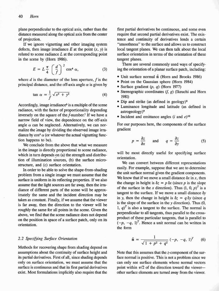
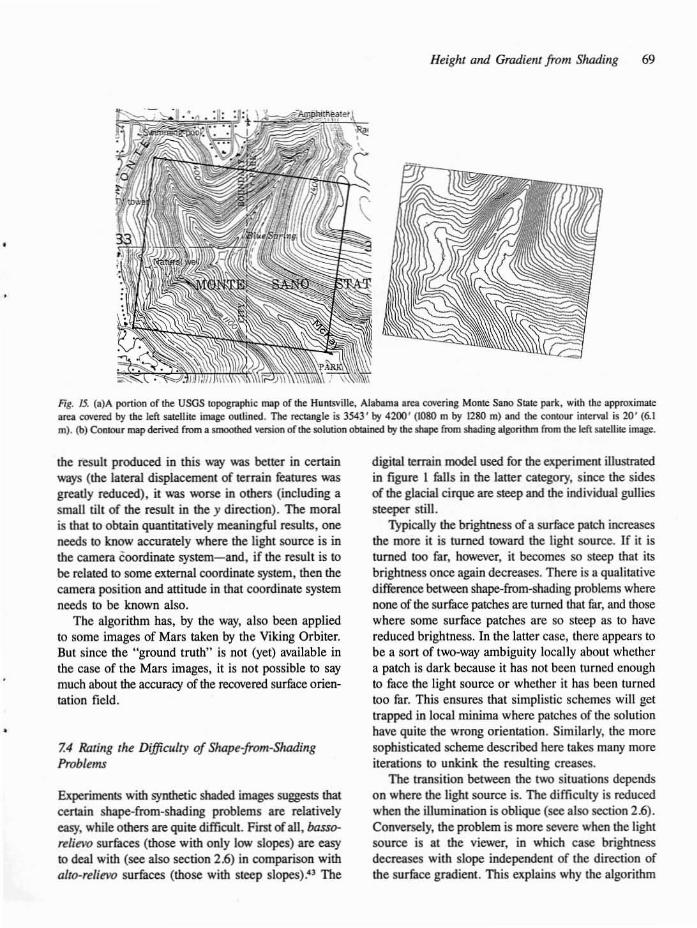
The new scheme was tested on a number of syntheticimages of increasing complexily. including somegenerated from digital tenain models of steep. wrinkledsurfaces. such as a glacial eirque with numerous gullies.Shown in figure I(a) is a shaded view of a digital ter­rain model, with Iighting from the North.....csl. This isthe input provided 10 the algorithm. The underlying231xl78 digital terrain model was conSlructed from adetailed contour map, shown in figure 2. of Hunting­Ion ravine on Ihe eastern slopcs of Mount Washingtonin the White Mountains of New Hampshire.~ Shownin figure I(b) is a shaded vicw of the same digital ter­rain model with lighting from the northeas!. This is/lot aV'ailable 10 the algorithm, but is shown here 10 make

(b)

(d)

fig. 1. RttoroSHuC1ion of surfacc from shaded image. See 1C:Jl1.

Heighl and Gradiel/l jrom Shading 39

2 Review of Problem Formulalion

(I)

(2)

yy =[­

Zandx =j~

Z

not made in an optimal way. Similarly, these details mayperhaps be of lesser importance for real images, whcreother error sources eould dominate.

In the next few sections we review image formationand other elementary ideas underlying the usual for­mulation of the shape-from-shading problem.Photoclinometry is also brietly rcviewcd for the benefit01" researchcrs in machine vision who may not befamiliar with this field. We then discuss both theoriginal and the variational approach to the shape-from­shading problem. Readers familiar wilh thc basic con­cepts may wish to skip over this material and go directlyto section 5, wherc the llew scheme is derived. For addi­tional delails see chapters 10 and II in Robm Vision(Horn 1986) and the collection of papers, Slwpe jromSlwdillg (Horn and Brooks 1989).

The shape-from-shading problem is simplified if weassume that the depth range is small comparcd withthc distallee ofthe scene from the vicwcr (which is oflenthc case whcn we have a narrow rield of view. that is,whctl wc use a telephoto lcns). Then we have

for some constant 2 0• so that the projcctioll is approx­imately orthographie. In this ease il is eotlvenient toreseale the image coordinates so that we ean write x= X and y = Y. For work on shape from sh:tding itis also convenicnt to use z. heighl above some reference

2.1 !mage Projeclioll (Im! Image 1rradiwlcc

For many problems in maehinc vision it is eonvenient\0 use a camerfl-cemered coordinate system with theorigin aL the center of projection and the 2-axis alignedwilh thc optical axis (the perpcndicular from the eentcr01" projection to the image plane)~. We can align the X­and Y-axes with the image plane x- and y-axes. Let theprillcipaf dis/(Jl1ce (that is, the perpendicular distancefrom the center of projection to the image plane) bc;; and let the image plane be reficcted through the centeror projcction so as to avoid sign reversal of the coor­dinates. Then the perspective projection equations are

Ag. 2. ConlOur map from which Ihc dilliwl lerrain model us.:d 10sylllhcsizc fillurcs l(a) and (b) "'as inlcrpolalcd. The surfacc \\"a,modclcd as a lhin pinte conSlrnincd 10 pass lhrough the contours at

lhe spccificd e1cv;llions. The intcrpolating surfacc WJS found b)' solv­ing lhe biharll10nic equalion. as describcd at lhe end of scclion 5.4.

apparent features of the surface thai may not stand outas weil in thc other shadcd view. Figurc l(c) shows ashaded view ol' the surl'ace reconstructed by thcalgorithm, with Iighting from the northwest-it matchesFigure I(a) exactly. More importantly, the shaded viewof the reconstructed surface with lighting from thenonheast, shown in figure l(d), matches figure I(b)cxactly also.3

With proper boundary conditions, thc new schcmerecovcrs surface orientation exUf..·/!y whcn prcscnledwith noise-free synthetic scenes4. Previous iterativeschemes do not find the exact solution, and in laetwander away from the correet solution when it is usedas the initial guess. To obtain exact algebraie solutions,seveml details of thc implcmcntalion have to be eare­fully thoughl through, as discussed in section 6. Sim­ple surfaces are casier to process-with good resuhscven when seveml ol' the implcmentation choices are

40 Horn

where d is the diameter of the Jens aperture, fis Iheprincipal distance, and the off-axis angle a is given by

(5)0,

q =­oy02oxp

first partial derivatives be continuous, and some evenrequire that second partial derivatives exist. The exis­tence and continuity of derivatives lends a cerrain"smoothness" to the surface and allows us to constructlocal tangent planes. We can then talk about the localsurface orientation in terms of the orientation of thesetangent planes.

There are several commonly used ways of specify­ing the orientation of a planar surface patch, including:

• Unit surface normal ii (Horn and Brooks 1986)• Point on the Gaussian sphere (Horn 1984)• Surfacc gradient (p, q) (Horn 1977)• Stereographic coordinates if, g) (Ikeuchi and Horn

1981)• Dip and strike (as defined in geology)8• Luminance longitude and latitude (as defined in

astrogeology)9• Incident and emittance angles (i and e)10

For our purposes here, thc componcnts of the surfacegradient

will be most directly useful for specifying surfaceorientation.

We can convert between different representationscasily. For example, suppose that we are to determinethe unit surface normal given the gradient components.We know Ihat ifwe move a small distance ax in x, thenthe change in height is oz = pax (since p is the slopeof the surface in the x direction). Thus (I, 0, p)T is atangent to !he surface. If wc movc a small distance oyin y, then the change in height is öz = q oy (since qis the slope of the surface in the y direction). Thus (0,I, ql is also a tangent to the surface. Thc normal isperpendicular to a11 tangents, Ihus parallel to the cross­product of these particular tangcnts, that is parallel to(-p, -q, I)T. Hence a unit normal can be written inthe form

(3)

(4)Itana =-,Jx2 +y2f

plane perpendicular to the optical axis, rather than thedistance measured along thc optica1 axis from the centerof projection.

If we ignore vignetting and other imaging systemdefects, then image irradiance E at the point (x, y) isrelated to scene radiance L at the corresponding pointin the scene by (Horn 1986).

, [dJ 2E=L- - cos4 a4 f .

Accordingly, image irradiance6 is a multiple ofthe sceneradiance, with Ihe factor of proportionality dependinginverselyon the square of Ihe f-number.' If we have anarrow field of view, thc dcpendence on the off-axisangle a can be neglected. Allernatively, we can nor­malize the image by dividing the observed image irra­diance by cos4 a (or whatever Ihe actual vignetting func­tion happens to be).

We conclude from the above that what we measurein the image is directly proportional to scene radiance,which in turn depends on (a) the strength and distribu­tion of illumination sources, (b) the surface micro­structure, and (c) surface orientation.

In order to be able to solve the shape-from-shadingproblem from a single image we must assume that thesurface is uniform in its reflecting properties. If we alsoassume that the light sources are far away, then the irra­diance of different parts of the scene will be approx­imately the same and the incident direction may betaken as constant. Finally, ifwe assume that the vieweris far away, then the direction to the viewer will beroughly the same for a11 points in the scene. Given theabove, we find Ihat the scene radiance does not depcndon the position in space of a surface palch, only on itsorientation.

Note that this assumes that the z-component ofthe sur­face normal is positive. This is not a problem since wecan only see surface elements whose normal vectorspoint within 1r/2 of thc direction toward the viewer­other surface elements are turne<! away from the viewer.

2.2 Specifying Sulface Orientatioll

Methods for recovering shape from shading depend onassumptions about the continuity of surface height andits partial derivatives. First of a11, since shading dependsonly on surface orientation, we must assume that thesurface is continuous and !hat its first partial derivativescxist. Most formulations implicitly also require that the

n ---r,=,=~=::i' (- p. - q. I)',JI+p2+ q2

(6)

Height and Gradient from Shading 41

2.4 Image Irradiance Equation

We are now ready to write the image irradianceequation

We can use the same notation 00 specify the direc­tion to a collimated light source or a small ponion ofan extended source. We simply give the orientation ofa surface element that lies perpendicular to the inci­dent light rays. So we can writell

E(x, y) = ~R(p(x, Y), q(x, y)) (9)

as long as the numerator is positive, otherwise R(p, q)=0.

We can show the dependence of scene radiance on sur­face orientation in the form of a reflectance map R(p,q). The reflectance map can be depicted graphicallyin gradient space as aseries of nested contours of con­stant brightness (Horn 1977, 1986).

The reflectance map may be determined experimen­taUy by mounting a sampie of the surface on agoniometer stage and measuring its brightness undcrthe given iIluminating conditions for various orienta­tions. Ahernatively, one may use the image ofa calibra­tion object (such as a sphere) for which sunace orien­tation is easily ca1culated at every point. Finally, areflectance map may be derived from a phenomeno­logical model, such as that of a Lambenian sunace.In this case one can integrate the prodoct of the bidirec­tional refleetance distribution fimetion (BRDF) and thegiven distribution of source brightness as a functionof incident angle (Horn and Sjoberg 1979).

An ideal Lambertian surface illuminated by a singlepoint source provides a convenient example of a reflec­tance mapl3. Here the scene radiance is given by R(p,q) = (Eohr) cos i, where i is the incident angle (theangle between the surfitce normal and the directiontoward the source), while Eo is the irradiance from thesource on a surface oriented perpendicular to the inci­dent rays. (The above formula only applies when i :s:-rfl; the scene radiance is, of course, zero ror i > -rfl.)

Now cos i = n's,so

for same PI and 91"

2.3 Reflecrance Map

(10)E(x, y) = R(P(x, y), q(x,)'))

E(x, y) = R(,.<x, y), l~X, y» (11)

2.5 Reflectance Map Linear in Gradienl

where p "" z" and q = Zy are the first partialderivatives of z with respect to x and y. This is a first­order partial differential equation; one that is Iypicallynonlinear, because the reflectance map in mOSI casesdepends nonlinearly on the gradient.

or

where E(x, y) is the irradiance at the point (X, y) inthe image, while R(p, q) is the radiance at the cor­responding point in the scene, at which p = p(x, y)and q = q{x, y). The proponionality factor f3 dependson the f-number of the imaging system (and may in­c1ude a scaling factor that depends on the units in whichthe instrument measures brighlness). h is customaryto rescale image irradiance so that Ihis proportionalityfactor may be droppcd. If the reflectance map has aunique global extremum, for example. then the imagecan bc normalized in this fashion, providcd that a pointcan be located that has the corresponding surface orien­tation. l •

Scene radiance also depends on the irradiance ofthe .scene and a reflectance factor Ooosely called albedobere). These faetors of proportionality can be combinedinto one that can be laken care of by normalization ofimage brightness. Then only the geometric dependenceof image brighmess on surface orientation remains inR(p, q), and we can write the image irradiance equa­tion in the simple form

Viewed from a sufficiently great distance, the materialin the maria of the moon has the interesting propertythat its brightness depends only on luminanee Iongitude,being independent of luminance latitude (Hapke 1963,1965). When luminance 10ngitude and latitude arerelated to the incident and eminance angles, il is fouodthat longitude is a funetion of (cos i/cos e). From the

(7)

1 + PIP + qlq (8)

+p1 +q2.JI+p:+q:

,7=~='"(-p" -q" I)TJI+p:+9:

E"-r .J I

s =

R(p, q)

42 Horn

10 obtain

(19)I,. = z,. - cg'(n - cy).

2.6 Low Gradiem Termi" ami Oblique JIlwllilla/ioll

z(x, y) = z(x, y) + g(n - cy) (18)

for an arbitrary function g! This is true because

z" "" z" + sg '(sx - cy)

ep+sq=cp+sq (20)

where p = i" and q = z,. It follows that R(p. q) =R(p, q). This ambiguity ean bc removcd if an initialcur\'e is given (rom which the profiles can be staned.Such an initial curve is lypically nOI available in prnc­tice. Ambiguity is nOI restricted 10 the special ease ofa reflectance map!hat is linear in thc gradient: Withouladditional constrainl shape-from-shading problemstypically da not have a unique solution.

so

Note that we obtain profiles of the surfaee by inle­grating along predetermined straight lines in the im­age. Each profile has its own unknown constam of in­tegralion. so there is a great deal of ambiguity in Iherecovery of surface shape. In fact, if z(x. y) is a solu­tion, so is

(16)

(13)

(14)

R(p, q) = f(ep + sq)

cp + sq "" rl(E(x, ynThe slopc in the image direction (e. s) is

for same functionfand some coefficients c and s. 80thLommel-Sceliger"s and Hapkc's funetions fit this mold(Minnaert 1961; Hapke 1963, 1965). [For a few otherpapers on the refleeting properties of surfaces, see(Hapke 1981, 1984; Hapke and WeHs 1981) and thebibliography in (Horn and Brooks 1989).] We can,without lass of generality, arrange for Cl + SI = 1.1'

If the functionfis continuous and monotonie.li wccan find an inverse

111 "" cp + sq "" I rl(E(x, y» (15).JC2 +S2 .JCZ+s2

Wc can imegralell oul this slope along the line

xm "" Xo + cE" 'and ym = )'0 + sE"

above we see thai cos i = ii . S, while cos e = ii . V,where v = (0. 0, I)T is a unh veclor in the directiontoward the viewer. Consequently,

cosi n's I--=-= (I+Psp+qsq) (12)cose n'Y ./1 +p}+q}

Thus (cos ilcos e) dcpcnds linearlyon the gradient com­ponenls p and q, and we can write

(17)z(!) = z, + I r' r' [E(x(,), y(,lll d,./ c2 +sd o

An extension of the above approach allows one to takeinto aecount perspcctive projection as weil as finitedistance to the light souree (Rindfleisch 1966). Twochangcs need to be made; onc is that the reflectancemap now is no longcr independcnt of image position(sincc the direetions 10 the viewer and the sourcc varysignifielmtly); and the other is thaI the integral is forthe logarithm of thc radial distance from the center ofprojeetion, as opposed to distance measured parallel10 the optieal axis.

The above was thc first shapc-from-shading orphotoclinomctric problem evcr solved in other Ihan aheurislie fashion. The original formulation was eon­siderably more eomplex than describcd above, as theresull of the use of full pcrspcclivc projeclion, the lackofthc nOlion of anYlhing like the rcflectance mup, andthe use ofan objccl-cemercd coordinate system (Rind­fleisch 1966).

If we are looking at a surfacc where the gradient (p.q) is smal!, we ean approximale the refleetance mapusing series expansion:

R(p, q) ~ R(O, 0) + pRr(O, 0) + qR,,(O, 0) (21)

This approach docs not work when Ihe rcflcet:mee mupis rotationally symmelrie, sinee thc first-order termsthen drop out lS• If the illuminution is oblique. however,we can apply the method in the previous section 10 geta first cstimate of the surface. Letting c = Rp(O, 0)..\" = Rq(O, 0) and

r' (E(x, Yll = E(x, y) - R(O, 0) (22)

wc find thatI

,(0 = Z, + --n~~~o;;=~.J R~(O, 0) + R~(O. 0)

J:(E(X(,), )~,ll - R(O, Oll'" (23)

(For a related frcquency domain approach sec (pentland1988.)

One might imagine that the above would provide agood way to get initial conditions for an iterative shape­from-shading method. Unforlunately, this is not veryhelpful, because of the remaining ambiguity in the'direction at right angles to that of profile integration.Iterative methods already rapidly get adequate varia­tions in height along "down-sun profiles," but thenstrugglc for a long time to try to get these profiles tiedtogether in the direction at right angles.

The above also suggests that errors in gradients ofa computed solution are likely to be small in the direc­tion toward or "away from" the source and large in thedirection at right angles. It should also be clear thatit is relatively easy 10 find solutions for slowly un­dulating surfaces (where p and q remain small) withoblique illumination (as in Kirk 1987). It is harder todeal with cases where the surface gradient varieswidely, and with cases where the source is ncur theviewer (see also the discussion in section 7.3).

3 Brief Review of Photociinometry

Photoclinometry is the recovery of surface slopes fromimages (Wilhe1ms 1964; Rindfleisch 1966; Lambiotteand Taylor 1967; Watson 1968; Lucchitta and Gambell1970; Tyler, Simpson, and Moore 1971; Rowan,McCau1ey, and HolJTl 1971; Bonner and Schmall 1973;Wi1dey 1975; Squyres 1981; Howard, Blasius, and Cutt1982). Many papers and abstracts relating to this sub­ject appear in places that may seem inaccessible tosomeone working in machine vision (Davis, Soder­b10m, and Eliason 1982; Passey and Shoemaker 1982;Davis and McEwen 1984; Davis and Soderblom 1983,1984; Malin and Danielson 1984; Wilson et al. 1983;McEwen 1985; Wilson, Hampton, and Baien 1985).(For additional references see Horn and Brooks 1989.)Superficially, pllOtoclinomellY may appear 10 be justanother name for slwpefrom shading. Two differentgroups of researchers indepcndenl1y tackled the prob­lem of recovering surface shape from spatial brightnessvariations in single images. Astrogeologists and workersin machine vision became aware of each other's interestsonlya few years ago. The under1ying goals ofthe twogroups are related, but there are some differences inapproach that may be worthy of abrief discussion.

3.1 Phoroclinometry !'ersus Shape [rom Shading

• First, photoclinometry has focused mostly on pro­file methods (photoclinomelrists now refer to existing

Height alld Gmdiellt [rom Slwding 43

shape-from-shading methods as urea-based photo­c1inometry, as opposed to projile-based). This cameabout in large pan because several of the surfacesof interest to Ihe aSlrogeologist have reflecting pro­perties that allow numerical integration alongpredetermined lines in the image, as discussed abovein section 2.5 (Rindfleisch 1966). Later, a similarprofile integration approach was applied to otherkinds of surfaces by using strang assumptions aboutlocal surface geometry instead. The assumption thaithe surface is locally cylindricalleads to such a pro­file integration scheme (Wildey 1986), for example.More commonly, however, it has been assumed thaithe cross-track slope is zero, in a suitable object­centered coordinale sySlem (Squyres 1981). This maybe reasonable when one is considering a cross-sectionof a linearly extended feature, like aridge, a graben,or a central section of a rotalionally symmetrie featurelike a crater.

• The introduction of conSlraints that are easiest to ex­press in an object-centered coordinate system leadsaway from use of a camera-centered coordinatesystem and to complex coordinate Iransformationsthat tend to obscure the underlying problem. Aclassic paper on photoclinometry (Rindfleisch 1966)is difficult to read for this reason, and as a resuh hadlittle impact on the field. On the other hand, it mustbe acknowledged that Ihis paper dealt properly withperspective projection, which is important when thefield of view is large. In all bul the earliest work onshape from shading (Horn 1970, 1975), Ihe assump­tion is made that the projeclion is approximately or­thographie. This simplifies the equations and allowsintroduction of the reflectance map.

• The inherent ambiguity of the problem does not standout as obviously when one works with profiles, asit does when one tries to fully reconstruct surfaces.This is perhaps why workers on shape from shadinghave been more concerned with ambiguity, and whythey have emphasized the importance of singularpoims and occluding boulldaries (Bruss 1982; Deiftand Sylvester 1981; Brooks 1983; Blake, Zisserman,and Knowles 1985; Saxberg 1988).

• The recovery of shape is more complex than the com­putation of a sei of profiles. Consequently much ofthe work in shape from shading has been restrictedto simple shapes. At the same lime, there has beenextensive lesting of shape from shading algorithmson synthetic data. This is something that is impor-

44 Hom

Ian! for work on shape from shading, but makes littlesense for the study of simple profile methods, exeeptto test for errors in the procedures used for inveningthe photomelric function.

• Shape-from-shading methods easily deal with arbi­trary colleetions of collimated light sources andeXlended sources, sinee these can be accommodatedin the reflectance map by integrating the BRDF andthe souree distribution. In astrogeology there is onlyone source of light (if we ignore mutual illumina­tion or interfleclion between surfaces), so methodsfor dealing with multiple sources or exlcnded sourceswere nOI developed.

• Calibration objects are used both in photoclinomelryand shape from shading. In photoclinometry the daladerivcd is used 10 fil parameters 10 phenomcnologica.lmodels sueh as those of Minnaen, Lamme! andSeeliger, Hapkc, and Lamben. ln werk on shape fromshading the numerical data is at times used direcllywithout furthercurve fitting. The parameterized modelshave the advantage that they permit extrapolation ofobservations to situations not encountercd on the eali­bration objeeL This is not an issue if the calibrationobjeet eontains surfaee elements with all possibleorientations, as it will if it is smooth and eonvex.

• Normalization of brightness measurements is treatedslightly differently too. Ifthe imaging device is linear,onc is looking for a single overall scale faetor. Inphotoclinometry this factor is often estimated by Jook­ing for a region thai is more or less flat and hasknown orientation in the object-eentercd coordinatesystem. In shapc from shading the brightness ofsingular points is often used to normalizc brightnessmeasurements instead. The choice depends in parton what is known about the scene, what the shapesof the objects are (that is, are singular points oroccluding boundaries imaged) and how the surfaeereneets light (Ihat is, is there a unique globalextremum in brighlness).

• Finally, simple profiling methods usually only requireeontinuity of the surface and existence of the firstderivative (unless there is an ambiguity in the inver­sion cf the photometric function whose resolution re­quires !hat neighboring derivatives are similar). Mostshape-from-shading methods require continuous firstderivatives und the existenee of second derivatives.(In some cases use is made of the equality of the sec­ond cross-deriV'dtives taken in different order, thatis, l.<y = Zy.<)' This means that these methods do not

werk weil on scenes eomposed of objects that areonly piecewise smooth, unless appropriatelymodified-but see (Malik and Maydan 1989).19

3.2 Profiling Methods

We have seen in section 2.5 how special photometrieproperties sometimes allow one to ealculatc a profileby imegration along predetermined straight lines in theimage. The other approach commonly used inphotoclinometry to pcrmit simple integration is to makestrong assumplions about lhe surface shape, most com­monly thal, in a suitable objecH;entered coordinatesystem, the slope of the surfaee is zero in a direetionat right angles to the direction in whieh the profile isbeing computed. Local surface orientation has twodegrees of freedom. 1be measured brightness providesone constraint. A second eonstraint is needed to ob­tain a solution for sunace orientation. A known tangentof the surface can provide the needed information. Twocommon cases are treatcd in astrogeology:(a) features that appcar to be linearly extended (such

as some ridges and grabens), in a direction pre­sumed to be "horizontal" (that is, in Ihe averagelocal tangem plane);

(b) features thai appear 10 be rotationally symmetric(Iike eraters), with symmetry axis presumed to be"venical" (thai iso perpendicular to the averagelocal tangem plane).

In eaeh ease, the profile is taken "'across" the feature,Ihal is, in a direction perpendieular to the imersectionof Ihe surfaee with the average local tangem plane.Equivalenlly, it is assumed that the cross-track slopeis zero in the object-eentered coordinate system.

One problem with this approach is that we obtaina profile in a plane containing the viewer and the lightsouree, nOI a "vertical" profile, one that is pcrpcn­dicular to the average local tangent plane. One way todeal with this is to iteratively adjust for the imagedisplacement resulting from f1uetuations in height onthe sunace, using first a sean that reaJly is just a straightline in the image, then using the eslimated profile 10introduce appropriate lateral displacements into the seanline, and so on (Davis and Soderblom 1984).

1t turns out that the standard photoclinometric pro­file approach can bc easily generalizcd to arbitrarytangent directions, ones that need not be pcrpendicularto the profile, and also 10 nonzero slopcs. All that we

Hejght and Gradient from Shading 45

(29)

(28)

(30)

(25)

oq "" Ey ö~

öq "" söx + toy (26)

,"d

an<!

y=Rq, z=pRp+qRq

p=E.., q""Ey

öz=pöx+qöy

then, from equations (26) and (Zl) we have

This is Ihe whole "trick." We can summarize the abovein the sei of ordinary differential equations

At this point we exploit the fact lhal we are free tochoose the direction of the step (&.r, hy). Suppose lIlatwe pick

op "" röx + soy

where r "" Z.u' S = z.ry = zyx, and t "" z», are Ihe sec­ond parlial derivatives of the height. It seems thai weneed to now keep track of the second derivatives also,and in order to do that we need the third panialderivatives, and so on.

To avoid this infinite recurrence, we take anotherlack. Note that we have not yet used the image irra­diance equation E(x, y) = R(p, q). To find thebrightness gradient we differentiale this equation withrespect to x and y and so obtain

So, as we explore the surface, we need to keep trackof p and q in addition to x, y, and z. This means thatwe also need to be able to compute the changes in pand q when we lake the step. This can be done lIsing

basic idea is quite easy 10 explain using the reflectancemap (Horn Im, 1986). Suppose Ihat we are at a point(x, y, Z)T on the surface and we wish to extend thesolution a small distanee in some direction by takinga step &.r in x and öy in y. We need to compute thechange in height öz. This we can do if we know thecomponents of the gradiem, p = z.. and q = z,..because

(24)ap+bq=c

This, together with the equation E = R(p, q), con­stitutes a pair of equations in the two unknowns p andq. There may, however, be more than one solution (orperhaps none) since one ofthe equations is nonlinear.Othcr means must be found 10 remove possible am­biguity arising from Ihis circumstance. Under appro­priate oblique Iighting conditions, there will usually on­Iy be one solution for most observed brighmess values.

From the above we conclude that we can recoversurface orientation locally if we assume that the sur­face is cylindrical, with known direction of thegenerator. We can integrale out the resulting gradientin any direction we please, not necessarily across thefeature. Also, the generator need not lie in the averagelocal tangenl plane; we can deal with other sirualions,as long as we know ,the direction of the generator inthe camera-centered coordinate system. Furthergeneralizalions are possible, since any means of pro­viding one more constraint on p and q will do.

In machine vision too, some workers have usedslrong local assumptions abaut the surface to allowdircct recovery of surface orientation. For example, ifthe surface is assumed to be locally spherical, the firsttwo partial derivatives of brightness allow one [0 reeoverthc surface orientation (pentland 1984; Lee andRosenfeld 1985). Ahernalively, one may assurne thatthe surface is locally cylindrical (Wildey 1984, 1986)10 resolve the ambiguilY present locally in the generalcase.

4 Review of Shape-from-8hading Schemes

need 10 assume is lIlal the surface can locally be ap­proximated by a (general) cylinder, that is, a surfacegenerated by sweeping a line, the genuator, along acurve in space. Suppose the direction of the generatoris given by the veetor t = (0, b, C)T. Note lIlat at eachpoint on the surface, a line parallel to the generator istangent 10 the surface. Then, sioce the normal is perpen­dicular to any tangent, we have I . n = 0 at every pointon the surface, or just

4.1 Chamcteristic Strips

The original solution of the general sbape from shadingproblem (Horn Im, 1975) uses the method ofcharaeteristic strip expansion for first order partial dif­ferential equalions (Garabedian 1964; John 1978). The

where the dot denotes differentiation with respect to~, a parameter lIlat varies along a panicular solutioncurve (the equations can be rescaled 10 make thisparameter be arc length). NOIe thai we acrually havemore than a mere chamcteristic curvt, since we alsoknow the orientation of the surface al all points in thiscurve. This is why a panicular solulion is called a

46 Horn

eharaeteristie strip. The projection of a eharacleristiccurve inlo Ihe image plane is ca11ed a base duzraeteristic(Garabedian 1964; lohn 1978).

The base eharacteristics are predetermined straightlines in Ihe image only when Ihe ratio x:y = Rp : Rq

is fixed, !hat is when Ihe reflectance map is linear inp and q. In general, one eannot integrate along arbiuarycurves in Ihe image. Also, an inilial eurve is neededfrom which to sproul Ihe eharacteristics strips.

It turns out that direcl numerieal implementauonsof the above equations do not yield particularly goodresuhs, since Ihe palhs of Ihe characleriSlics are affectedby noise in the image brightness measurements anderrors lend to accumulate along Iheir length. In partic­ularly bad eases, the base characteristics may evencross, which does not make any sense in lerms of sur­face shape. It is possible, however, to grow eharaeter­istic strips in parallel and use a so-called sharpeningprocess to keep neighboring charaeleristics eonsistentby cnforcing Ihe condilions 4 = P x, + q Y, and E(x,y) "" R(p, q) along curves connecting Ihe tips ofcharacteristics advancing in parallel (Horn 1970, 1975).This greatiy improves the accuracy of Ihe solulion, sincethe computation of surface orientalion is lied morec10sely 10 image brightness itself ralher Ihan 10 Ihebrightness gradient. This also makes it possible to inter­polate new characteristic strips when existing onesspread too far apart, and to remove some when Iheyapproach each olher 100 ciosely.

4.2 Rotationally Symmetrie Refleetance Maps

for some k. That is, in Ihis casc the eharaeteristies arecurves of sleepest ascenl or descent on Ihe surfaee. Theextrema of surface heighl are sources and sinks of ehar­aeteristic curves. In this ease, diese are the points whereIhe surface has maxima in brightness.

This example illustrates the importance of SO'<:allcdsingular points. At most image points, as we have seen,Ihe gradient is not fully constrained by image bright­ness. Now suppose Ihal R(p, q) has a unique globalmaximum,zo Ihal is

A singular point (xo, Yo) in the image is a point where

(35)

At such a point we may conclude that (p, q) = (Po,qo). Singular points in general are sources and sinksof characteristie eurves. Singular points provide slrongconstraint on possible solutions (Horn 1970, 1975; Bruss1982; Brooks 1983; Saxberg 1988).

Tbe occludjng boundary is the set of points whereIhe local tangent plane contains Ihe direclion towardIhe viewer. It has been suggested Ihal occluding boun­daries provide strong conslrainl on possible solutions(Ikeuchi and Horn 1981); Bruss 1982). As a conse­quenee there has been inleresl in representations forsurface orientalion that behave v..-ell ncar Ihe occludingboundary, unlikc Ihe gradient which becomes infinile(lkeuehi and Horn 1981; Horn and Brooks 1986).Rceently Ihere has been some question as to how muchconslraint occ1uding boundaries really provide, givenIhal singular points appear to already slrongly conslrainIhe solution (Brooks 1983; Saxberg 1988).

and so thc direclions in which Ihc base characleristicsgrow are given by

One ean get some idea of how the charactcrislics ex­plorc a surface by considering Ihe special easc of a rota­tionally symmelric reflectancc map, as mighl applywhcn thc light source is at the viewer (or when deal­ing wilh scanning e1cctron microscope (SEM) images).Suppose thai

R(p, q) = f(Pl + ql)

4.3 Existeflee and Ulliqueness

Queslions of existenee and uniqueness of solutions ofthe shape·from-shading problem have slill not bcenresolvcd enlircly satisfactorily. Wilh an initial curve,however, the melhod of eharacleristic strips docs yielda unique solution, assuming only eontinuity of Ihe firslderivalives of surface heighl (see Haar's Iheorem onpg. 145 in Courant and Hilben 1962 or Bruss 1982).The queslion of uniquencss is more difficult [0 a-:swerwhen an inilial curve is nOI available. One problem isIhat il is hard 10 say anything eomplelely general thatwill apply 10 all possible reflcctance maps. More canbe said when spccific reflcetanee maps are chosen, suchas ones Ihal are linear in Ihe gmdienl (Rindfleisch 1966)or those Ihat are rotalionally symmetrie (Bruss 1982).(33)

(31)

y "" kqan<!i "" kp

thcn

Height alld Gradiem from Shading 47

It has recently been shown that there exist impossi­ble shaded images, that is, images that do not corres­pond to any surface illuminated in the specified way(Horn, Szeliski, and Yuille 1989), It may turn out that'almost a1l images with multiple singular points are im­possible in this sense (Saxbcrg 1988). This is an impor­tant issue, because it may help explain how our visualsystem sometimes determines that the surface beingviewed cannot possibly be uniform in its reflccting pro­perties. One can easily come up with smoothly shadedimages. for example, that do not yield an impressionof shape, instead appearing as flat surfaees withspatial1y varying reflectanee or surfaee "albedo," (Seealso figure 10 in section 7.2.)

In fact, the error can be made equal to zero for an in­finite number of choices for {p~r, y), q(x, y)}. We canpick out one of these solutions by finding the one thatminimizes some functional such as a measure of"departure from smoothness,"

II(p; +p} + q~ + q})drdy (39)

while satislJing the constraint E(x, y) = R(p, q). Intro­ducing a Lagrange multiplier Mx, y) to enforce the con­straint, we find that we have to minimizc

II«P.~ +p; +q~ +q;) + h(x,y)(E- R»drdy (40)

The Euler cquations are

4.4 l1:,riatiolla{ Formll{ations

where E(x, y) is the image irradiance at the point (x,y), while R(p, q), the refleclallce map, is the (normal­ized) scene radiance of a surface patch with orienta­tion specified by the partial derivatives

As discussed above in section 2.4, in the case of a sur­face with constant albedo, when both the observer andthe light sources are far away. surface radiance dependsonly on surface orientation and not on position in spaceand the image projection can be considercd to be or­thographie.21 In this case the image irradiance equa­tion becomes just

(41)

(43)

E(x, y) = R(p, q) (42)

IIp + Mx, y)R" = 0

Ilq + Mx, y)Rq = 0

Unfurtunately, no convergent iterative scheme has beenfound for this constrained variational problem (Hornand Brooks 1986); (compare Wildey 1975).

We ean approach this problem in a quite differemway using the "departure from smoothness" measurein a penalty term (lkeuchi and Horn 1981), looking in­stead for a minimum 0[24

After elimination of the Lagrange multiplier A(x, y),we are left with the pair of equations

IJ[(E(x, y) - R(p, q»)2

+ h(P; + p} + q; + q})]drdy

(36)

(37)azq =­ay

E(x, y) ,= R(P(x, y), q(x, y»

azp = ~ax

Using a discrete approximation of the Laplacianoperator2 '

It should be pointed out that a solution of this"regularized" problem is flor a solution of the originalproblem, although it may be dose to some solution ofthe original problem (Brooks 1985). In any case, thisvariational problem leads to the following coupled pairof second-order partial differential equations:

of surface height z(x, y) above some reference planeperpendieular to the optieal axis.

The task is to find z(x, y) given the image E(x, y)and the reflectance map R(p, q). Additional constraints,such as boundary conditions. and singular points, areneeded to ensure that there is a unique solution (Bruss1982; Deift and Sylvester 1981; Blake, Zisserman, andKnowles 1985; Saxberg 1988). Ifwe ignore imegrabil­ity,n some versions of the problem of shape fromshading may be considered to be ill posed,2l that is,there is not a unique solution (P(x, y), q(x, y)} thatminimizes the brighlness error

hllp -(E(x, y)

hllq = - (E(x, y)

R(p, q)) R,,(p, q)

R(p, q» R,(p, q) (44)

11 (E(x, y) - R(p, q»)2 clx dy (38) (45)

48 Hort!

wherejis a local average off, and (is the spacing be­tween picture cells,1' we arrive at the set of equations

I(X'Pu = I(X 'Pu + (E(x, y) - R(p, q» RpCp. q)

I(X' qu = I(X 'qu + (E(x, y) - R(p, q» R/'p, q) (46)

where X' = X1E2. This immediately suggests theiterative scheme

In general. this approach produces solutions that are100 smooth, with the amount of distonion dependingon the choice of lhe parameter A. For relaled reasons,this algorithm does weil only on simple smOOlh shapes,and does not perfonn weil on complex, wrinkJedsurfaces.

(E(x, y) - Rrp'°', q<o'»Rp(P'o" q<o')

q~7+1) = iiW + _1-,A'

for some constanl k. While this includes all harmoniefuoctions, it exeludes most real surfaces. for which ad­

justments away from the oorrCCI shape are needed 10

assure equality of lhe lef! and right sides of equations(44) describing the solUlion ofthe modified problem.

(E(x, y) - R(p(nl , q(n))Rq(p(nl, qln) (47)

where the superscript denotes thc iteration numberPFrom the above it may appear that R(p, q), R/.p,

q), and Rq(p. q) should be ewluated using the "old"valucs oep and q. iIlUms out that the numerical stabililyof the scheme is somewhat enhanced if they areewluated inSlead at the local average values, p and q(Ikeuchi and Horn 1981).

One might hope that the correct solution of theoriginal shape+from-shading problem provides a fixedpoint for the iterative scheme. This is not too likely,however, since we aie solving a modified problem !hatincludes a penalty tenn. Consequendy, an interestingquestion one mighl ask aboul an aigorithm such as this,is whether il will "walk away" from the correct solu­tion of the original image inadiance equation E(x, y)= R(p, q) when this solution is provided as an initialcondilion (Brooks 1985). The algorithm described heredoes just thai, since it can Irade off a smalJ amount ofbrightness error againsl an increase in surfaeesmoolhness. At the solution, we have E(x, y) = R(p,q). so that Ihe righl-hand sides ofthe two coupled par+tial differential equations (equatio!JS (44» are zero. Thisimplies that if the solulion of the modified problem is10 be equal the solution of the original problem thenthe Laplacians ofP and q must be equal 10 zero. Thisis the case for very few surfaces, jusl those for which

(53)

(51)

czol+szy=cp+sq

, , -

;Z 4J = (2 4I ~ (Pol + q,),

a set of equations that suggeslS the following iterativescheme:

where (c, s) is a nonnal to the boundary.29Another way ofdealing with the integrabilily issue

is to try and directly minimize

,\;." ~ i~' - ~ ({P,)~' + (q,,}~') (52)•

tJ.z. = Pol + q, (50)

Using the discrete approximation of the Laplacian givenalxwe (equation (45» yields

where the tenns in braces are numerical estimates ofthe indicated derivatives at the picture cell (k, f).

Thc so-callcd natural boundary conditiolls here arejust

In any case, we are also still faced with the problemof dealing with the lack of imegrability. thai is the lackof a surface z(x, y) such that p(x, y) = zol(x, y) andq(x, y) = Zy(x, y).28 At the very least, wc should tryto find the surfacc z(x, y) that has panial derivativeszol and Zy that come e10sest to mate hing thc computcdp(x, y) and q(:c, y), by minimizing

JJ«zol - pp + (z, - qP) dx (Iy (49)

This leads to the Poisson equation

4.5 Rt!COvering Height from Gradient

ff ((E(x, y) - R(p, q»' + A(P, - q,)'} dxdy (54)

This leads to the coupled partial differential equations(Horn and Bmoks 1986)

A(PJY - qSJ) = - (E(x, y) - R(p. q»Rp

Mq" - p,,) ~ - (E(x, y) - R(p, q»R. (55)

(48)dz(x, y) = k

Height and Gradient from Shading 49

and we know from the previous section lhal the Eulerequation for this variational problem is jusl

We now have one equation for each of p, q, and z.These three equations are c1early satisfied when p

= zr, q = z, and E = R. That is, if a solution of theoriginal shape-from-shading problem exists, then itsatisfies this system of equations exaetly (which is morethan can be said for some other syslems of equalionsobtained using a varialional approach. as pointed OUIin seclion 4.4). It is instruclive to substilute the expres­sions obtained for p and q in Pr + q,:

Pr + q, = Z.u + Z,)"

I+ - [(E - R)(Rpppx + Rpq(p, + q,)

"+ Rqfl,.) - (RIP" + R"Rq(p, + qr)

+ R~,) + (Eß, + E,Rq» (60)

Since liz. = (Pr + q,), we ROte that the three equationsabove are salisfied when

This sei of equalions can also be discrelized by intro­ducing appropriate finite difference approximations lOrthe second partial derivatives Pyy' q;cr and the crossderivatives ofP and q. An iterative scherne is suggestedooce one isolates the cenler terms of the discrele ap­proximations ofpyy and q;cr. This is very similac to themethod developed by Stral, although he arrived at hisscheme directly in the discrete domain (Strat 1979). Hisiteralive scheme avoids the excessive smoothing of theone described earlier, but appears to be less stable, inthe sense thai it diverges under a wider set ofcircumstances.

5 New Coupled Height and Gradient Scheme

The new shape-from-shading scherne will be presentedthrough aseries of increasingly more robust variationalmethods. We start with the simplest, which growsnalurally out of whal was discussed in the previousseclion.

4z=Pr+q, (59)

5./ Fusing H~ight and Gradient Recovery

One Wi!'j of fusing the TeCCJ'Yery oe grad ienl from shadingwith the recovery of heighl from gradienl, is 10 repre­sent both gradient (p, q) and height z in one variationalscheme and to minimize the funetional

ff [(E(x, y) - R(p, q))'

+ /.l«zx - pp + (z, - q)2)] dx dy (56)

Note Ihal, as far as p{x, y) and q{x, y) are concerned,Ihis is an ordinary calculus problem (since no partialderivalives of P and q appear in the inlegrand). Dif­fercntiating the integrand with respect to p{x, y) andq(x, y) and setting the resull equal to zero leads to

Ip=zx+-{E-K)R,

"Iq=z,+-(E-K)R" (57)

"Now z{x, y) does not oceur dircctly in (E{x, y) - R(p,q» so 'Ne actually just need 10 minimize

(Rj,pr + RpR,,(P, + qJ + Rl,q,)

- (E,Rp + E,R.)

- (E - K)(R",P. + R",,(p, + q,) + R.,q,) (61)

This is exaetly the equalion obtained at the end of sec­lion 4.2 in (Horn and Bmoks 1986), where an attemplwas made 10 dircctly impose integrability using the con­slraint P, = qr. It was stated there thai no convergenlilerative scheme had bcen found for dircctly solvingthis complicated nonlinear partial differential cquation.Thc mcthod presented in this scction provides an in­direct way of solving this equation.

Nole thai the natural boundary conditions for z areonce again

CZr + sz, = cp + sq (62)

where (c, s) is anormal to the boundary.The coupled system of equations above for p, q

{equation (57» and z (equalion (59» immedialely sug­gests an iterative scheme

Pti+l) = (zrlti) + .!. (E - K)R,

"11tH

) = (z,}17) + .!. (E - R)R"

"

50 Horn

(63)which point lhe penalty term is removed in order toprevent it from distorting lhe solution. We first Ireatthe Iinearization of the reflectance map.

5.2 lineariUllion 01 Reflectance Map

Again, galhering all of the terms in Pi! and q.l:l on theleft-hand sides of lhe equations, we now obtain

R(p. q) ... R(po. qol + (p - pol Rp(Po. qo)

+ (q - qo) Rq(Po. qo) + . . (64)

This leads to

(p. + Rfi) OPtl + H,)?,Oqkl =Il oZx + (E - R)Rp

RpRq 0Pkl + (11 + R~) oqk/ = IJ. OZy + (E - R)Rq (67)

(66)

(68)

oqk/ = qk' - qo

OZ" = Zy - qo

and

and

D = Il(p. + R~ + R~)

while lhe equation for z rcmains unchangcd. (Note lhatnow R, Rp , and R, denOIC quantitics evaluated 31 thereference gradient (Po, qo).)

It is convenient to rewritc these equations in lermsof quantities relative to thc refcrence gradient (Po. qo).Let

We can develop a belter scheme lhan the one describedin lhe previous section, while preserving the apparentlinearity of the equations, by approximating lhe reflec­tance map R(p, q) locally by alinear funclion of P andq. 1bere are several options for choice of reference gra­dient for the series expansion. so let us keep it generalfor now at (Po. qO)'lO We have

(p. + R~)P.I:I + R"Rrfltl = Jl.Zx

+ (E - R + poRp + qoRq)Rp

RqR,p.l:l + (p. + R~) q.l:l = Jl.Zy

+ (E - R + poRp + qoRq)Rq(65)

(The equ31ions clcarly simplify somcwhat ifwe choose(z.r> Zy) for the rcference gradiem (Po, qo).) We canview the above as 3 pair of linear equations for Op.I:Iand Oqi/' The detcrminanl of thc 2 x2 coefficientmatrix.

0Pk/ = Ptl - Po

oZx=zx-Po

where we have used the discrete approximation of lheLaplacian for z introduced in equation (45). This newiterative scheme works weil when lhe initial valuesgiven for p. q. and z are elose to lhe solution. It willconverge 10 the exact solution if it exisls; lhat is, if lhereexisls a discrete set ofvalues {Zti} such lhat {P.l:l} and{q.l:l} are lhe discrete estimate of lhe first partialderivatives of z wilh respect tO.l" and y respectively andE.I:I = R(P.l:l. q.l:l)'

In lhis case lhe functional we wish 10 minimize canactually be reduced 10 zero. 11 should be apparent lhatfor lhis 10 happen. the discrete estimalor used for lheLaplacian must match the sum of the convolution oflhe discrete eslimalor of the.l" derivative wilh itself andlhe convolution of the discrete estimator of the yderivative wilh itself. (This and related mauers are lakenup again In section 6.2).

The algorithm can easily be tested using synthelicheighl data Z.tJ. One merely estimates lhe partialderivatives using suitable discrete difference formulas,and lhen uses lhe resuhing values Pil and q.l:110 com­pute the synthetic image E.I:I = R(P.l:l' q.l:l)' This con­struction guarantees thai lhere will be an exact solu­tion. If areal Image is used, there is no guarantee lhattherc is an exact solution, and lhe algorilhm can at bestfind a good discrete approxima!ion of lhe solution ofthe underiying continuous problem. In this case thefunctional will in fact not be reduced exactly to zero.In some cases the residue may be quite large. This maybe the result of aliasing introduced when sampling theimage. as discussed in section 6.5, or because in factthe image given could not have arisen from shading ona homogeneous surface with the reflectance propertiesand lighting as encoded in the reflectance map-thatis, it is an impossible shaded image (Horn. Szeliski.and Yuille 1989).

The iterative algorithm described in this section,while simple, is not very stable, and has a tendencyto gel stuck in local minima, unless one is elose to theexact solution, particularly when the surface is com­plex and the reflectance map is not elose to linear inthe gradient. It has been found lhat the performanceof this algorithm can be improved greatly by lineariz­ing lhe reflectance map. h can also be stabilized by add­ing a penalty term for departure from smoothness. Thisallows one to come elose to the correct solulion. at

Height arid Gradiell1 Iro", Shadillg 51

is always positive, so there is no problem withsingularities. The solution is given by

DOPt! = (p. + R~)A - R"RIJ

D ;qu ~ (p + RfilB - R,R"A (69)

where

A diserete approximation of these equations ean beobtained using the discrete approximation of the Lapla­eian operator introduced in equation (45):

-(E - R)Rp - p.(zx - Pu)

This leads to a convenient iterative scheme where thenew values are given by

in terms orthe old reference gradient and the incrementscomputed above. The new version of the iterativescheme does not require a great deal more computa­tion than the simpler scheme introduced in section 4.5,since the partial derivatives Rp and Rq are a1readyneeded there.

(74)

(75)

l: (it, - 41) :: Pol' + qy

where E, R, Rp, and Rq are the corresponding valuesat the picrure cell (k, 1), while 4.1" 4" P", and q, arediscrete estimates of the partial derivative of 4, P, andq there. We can collect the tenns in Pt!, qu, and Zu onone side to obtain

(KA' + IJ,)PI:! :: (KA 'PI:! + p.l.,,) + (E - R)Rp

(KA' + IJ)qt! :: (KA 'qu + p.l.,) + (E - R)Rq

K K_ (p )-41=-Zu- ,,+qEl El ,

(70)

A=IJ,Ozx+(E-R)Rp

B::IJOz,.+(E-R)Rq

5.3 !ncorporating Departure from Smoothness 'Tenn

The Euler equations of this calculus of variations prob­lem lead to the following coupled system of seeond­order partial differential cquations:

JJ[(E(x, y) - R(p, q))'

+ A(P} + p} + qi + qJ)

+ p.((z" - p)l + (z,. - q)l)JiUdy (72)

.We now introduce a penalty tenn for departure fromsmoothness, effcctively combining the iterative methodof (lkcuchi and Horn 1981) for recovering P and q fromE(x, y) and R(p, q), with the scheme for recovering zgiven P and q discussed in section 4.5. (For the mo­ment we do not linearize the reflectance map; this willbe addressed in section 5.6.) We look direetly for aminimum of

where A' = AIE l . These equations immediately suggestan iterative scheme, where the right-hand sides arecomputed using the current values of the Zu, Pt!, andql:!, with the resuhs then used 10 supply new values forthe unknowns appearing on thc left-hand sides.

From the above it may appear that R(p, q), Rp(p,q), and Rq(p, q) should bc evalualed using the "old"values ofP and q. One might, on the other hand, arguethat the local average values p and q, or perhaps eventhe gradient estimates 4" and 4)" are more appropriate.Experimentation suggests that the scheme is most stablewhen the loeal averages p and q are used.

The above scheme contains a penalty tenn for depar­ture from smoothness, so it may appear that it cannoteonverge (0 the exact solution. Indeed, it appears asif the iterative scheme will "walk away"' from the cor­rect solution when it is presented with it as initial con­dilions, as discussed in section 4.4. It turns OUI,however, that the penalty term is needed only to pre­vent instability when far from the solution. When weoome dose to the solution, A' can be reduced to zero,and so the penalty renn drops out. It is tempting 10 leavethe penalty tenn out right from the start, sinee thissimplifies the cquations a great deal, as shown in sec­tion 5.1. The contribution from the penalty tenn does,(73)

Af!,.p :: -(E - R)Rp - P.(4" - p)

~q :: -(E - R)Rq - ""(4,. - q)

.o.z = p" + q,.

52 Horn

however, help damp out instabilities when far from thesolution and so should be included. This is particularlyimportant with real data, where one cannot ex.pect tofind an exact solution.

Note, by the~, that the coupled second-order par­tial differential equations above (equation (76)) areeminently suited for solution by coupled resistive grids(Horn 1988).

5.4 RelOlionship to Existing Techniqlles

!!p\(p: +pJ. + q: + q;)

+ «z.. - p)2 + (Z,. - q)2)1 dr dyand arrives at the Euler equations

;. t>p ~ -(z, - p)

At:.q = -(Zr - q)

.6z = p.. + q,.

Now consider that

6("<) - t>(p, + q,)

(76)

(77)

(78)

0'

and so

(79)

(80)

Since application of the Laplacian operator and dif­ferentiation commute wc have

5.5 Boundary Condirions and Nonlinearity 01Reflectance Map

So far we have assumed that suitablc boundary condi­tions arc available, that iso the gradicnt is known on

>"t:.(t:,.z) = -.6z + (p.. + qr) = 0 (81)

So his rnethod solves thc biharmonic cquation for z:.by solving a coupled set of sccond-order partial dif­ferential equations. It does it in an elegant, stable waythat pennits introduction cfconstraints on both heightz: and gradient (p, q). This is a good method for in­terpolating from sparse dcpth and surface orienta­tion data.

The bihannonic equation has been employed to inter­polate digital terrain models (UfMs) frorn contourmaps. Such UfMs were used, for example, in (Horn1981; Sjoberg and Horn 1983). The obvious implemen­tations of finite difference approximations of thc bihar­manie operator, however, tend to be unstable becausesome ofthe weights are negative, and because thc cor­responding coefficient matrix lacks diagonaldominance. Also, the treaunent cf boundary conditionsis complicated by the fact that the support of the bihar­manie operator is so large. The scherne described abovecircurnvents hath of these difficulties-it was used 10

interpolate the digital terrain model uscd for the ex­ample illustrated by figure I.Jl

• Rccently, new methods have been developed thatcombine the iterative scheme discussed in section 4.4for recovering surface orientation from shading witha projection onto the subspace of intcgrablc gradients(Frankot and Chellappa 1988; Shao, Simchony, andChellappa 1988). The approach there is lo altematelytake one step of the iterative scheme Okeuchi andHorn 1988) and to find the "nearest" intcgrablegra~ienl. This gradient is then provided as initialconditions for the next step of the iterative scheme,ensuring that thc gradient field never dcparts far fromintcgrabiLity. The integrable gradient dosest to agiven gradient field can be found using onhononnalseries expansion and the fact that differentiation inthe spatial d..omain corresponds to multiplication byfrequency in the transfonn domain (Frankot andChellappa 1988).

• Similar results can be obtained by using instead themethod described in section 4.5 for recovering theheight z(x, y) that best matches a given gradient. Theresulting sunace can then be (numerically) differen­tiated to obtain initial values for p(x, y) and q(x, y)for the next step ofthe iterative scheme (Shao, Sim­chony, and Chellappa 1988).

• Next, note that we obtain the scheme of Okeuchi andHorn 1981) (who ignored the integrability problem)discussed in section 4.4, if we drop the departurefrom integrability term in the integrand-that is,when JL = 0. If we instead remove thedeparture fromsmoothness term in the integrand-that is, when A= O-we obtain sornething reminiscent of theitcrative scherne of (Strat 1979), although Strat dealtwith the integrability issue in a different way.

• Finally, if we drop the brighmess error tenn in theintcgrand, we obtain the scheme of (Harris 1986,1987) for interpolating from dcpth and slopc. Heminimizes

Height and Gradiem 170m Sitadillg 53

Ihe boundary of Ihe image region to which the COffi­pulation is to be applied. Ifthis is not thecase, the solu­tion is likely nOI to be unique. We may nevertheless­try to find some solution by imposing so-called IIaturalboundary conditions (Courant and Hilbert 1953). Thcnatural ooundary conditions for the variational problemdescribed here can be shown to be

Cls + $Z, = ep + sq (83)

where (e, s) is anormal to the boundary. That is, thenormal derivative of the gradienl is zero and the nor­mal derivative of thc height has to match the slope inthe normal dircction computed from the gradient.

In the above we have approximated thc original par­tial differential cquations by a set of discrete equations,threc for every picture cell (one eaeh for p. q, and ,).Ifthese equalions were linear, we eould directly applyall the e.xisting thoory relating to convergence of variousiterative schemes and how one soh'es such equationsefficiently, given that thc corresponding coefficientmatrixes are sparse.12 Unfortunatcly, the equations arein general not linear, bccause of the nonIineardependenee of thc reflectance map R(p. q) on the gra­dient. In fact, in deriving the above simple iterativcscheme, we' have treated R(p, q), and its derivatives,as constant (independent of p and q) during any par­tieular itcrative adjustmcm of p and q.

D = AN(A" + Rfi + R~) (88)

is always positive, so there is no problem withsingularities. The solution is given by

(89)

Dopu = (A" + R~)A

DOqkJ = (A" + Ri)B

while thc equation for z remains uochanged. (Note Ihathere R, Rp , and Rq again dcnolc quantities C\'aluatedat the referenec gradient (Po. qo». In the abovc wc haveabbreviated A~ = KA' + 11.

It is convcnienl to rewrite thcse equations in termsof quantities defincd relative to thc refercnce gmdiem:

0Pkt = Pu - Po and Oqu = qu - qo

0Pkl = Pkt - Po and oqu = qu - qo

oZs = Zs - Po and oZ.< = :, - qo (86)

This yiclds

(A ~ + Rfi)oPkl +RpRqoqk/ = KA'OPU

+ p.oz.. + (E - R)R1,

RpRqoqkJ +(A ~ +R~) Oqkl = KA'oqkJ

+I-l&y + (E - R)R'I (87)

(Thc equations c1carly simplify somcwhat ifwe chooseeither Pand qor Zs and " for the reference gmdicntPo and qo.) We can vicw thc abO\'e as a pair of linearequations for oPu and Oqkl' Thc determinant of the2 x2 coefficicnt matrix

eqs + sq, = 0 (82)andeps + sP, = 0

an<!

(84)

5.6 Locaf Linear Approximation of Reflectallce Map

In scclion 5.2 we linearizcd thc reflectanec map in orderto countcmct thc tendency of thc simple itcmtive schemedcvcloped in section 5.1 to get stuck in local minima.We now do the same for the more eomplex schemedescribcd in $Cetion 5.3. We again use

R(p, q) ,.. R(Po, qo) + (p - Po)Rp(Po, qo)

+ (q - qo)R,f.Po. qo) + ...

whcre

A = KA' 0Pkl + I-l oz.. + (E - R)Rp

B = Kh' oqt/ + 1-l0l>, + (E - R)Rq (90)

This leads to a convenient iterativc schcmc where thcnew ",ducs are given by

p~+l) = p~jl + op~l

'Il7'" ~ qt' + ",t'Gathering all of the terms in Pkt and qtl on the lef!·hand sidcs of thc equations, we now obtain

(A ~ + RiZ,)pk/ + R,,Rt/ltl

= (KA 'Pkl + J.lZ..•) + (E - R + poRp + qfftq)Rp

RqR,Pu + (A ~ + R~)qkl

= (KA 'qu + JLZ,) + (E - R + poRp + qoRq)Rq (85)

in terms ofthe old reference gradicnt and the incremcntseompUlcd abovc. It has been detcrmined cmpiricallythat this schcmc converges under a far widcr sct of cir­cumstances than the one prcscnlcd in the prcviousseClion.

Experimcntation with different rcfcrcnce gmdicnts.including the old values of fJ and q, thc local averagcPand ij, as weil as Zs and zr showed Ihat thc aeeuracy

54 Horn

of the solution and the convergence is affected by thischoice. It became apparent that if we do not want thescheme 10 "walk away" from the correct solution, thenwe should use the old value ofp and q forthe referencePo and qo· PIO Pu Pl2

6 Some Implementation Details Z10 Zl1

6./ Deril'Oti\'e Esrimators anti Slaggered GridsPoo Pol Po,

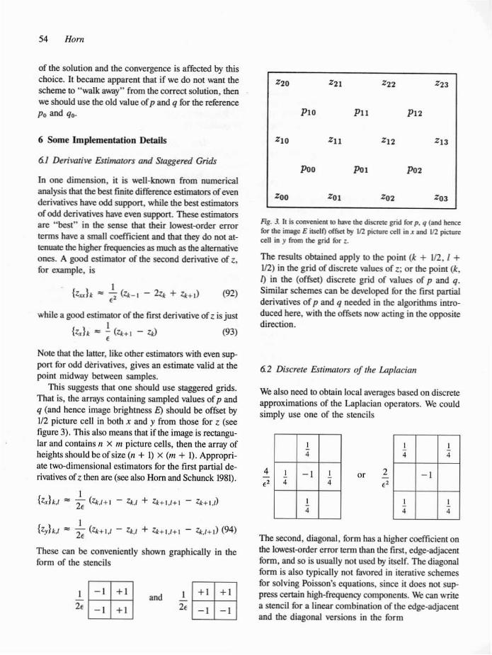
Fig. .1 11 i$ COllYC:llielll 10 haYC: thc: disctC:1C grid for p. q (and he:nce:lOr lhe: image E il$C:lf) otfsd by tI2 picture teil in.f lind tI2 pictureteil in y from the: grid lOr ~.

The results obtained apply 10 thc point (k + 112. I +1(2) in the grid of discrete values of Z; or the poim (k,1) in the (offset) discrete grid of values of p and q.Similar schemes can be developed for Ihe first partialderivatives of p and q needed in the algorithms imro­duced herc, with the offsels now acting in the oppositedirection.

In ODe dimension, il is well-known from numericalanalysis that the best finite difference estimators ofevenderivatives have odd support, while the best estimatorsof odd derivatives have even support. These estimatorsare "best" in the sense that their lowest-order errartenns have a small coefficient and that they do not at­terlUate the higher frequencies as much as the alternativeones. A good estimator of the second derivative of Z,for example, is

while a good estimator of the first derivative of l is just1{z.rh ... - (l,hl - W (93),

Zoo ZOI ZO' Z03

I I4 4

-1

I I4 4

20'

I4

I -1 I4 4

I4

4

We also need 10 obtain local averagcs bascd on discreteapproximations of Ihc Laplacian operators. We couldsimply use one of thc slencils

6. 2 Discrell! Eslimators 0/ fhe Loplaciafl

The second, diagonal, form has a higher cocfficienl onthe lowest-order error term Ihan Ihe first, edge-adjacemform, and so is usually not used by itself. Thc diagonalform is also typically not favorcd in iterative schemesfor solving Poisson's equations. since it does not sup-­press cenain high-frcquency components. We can writea stencil for alinear combination of the edge-adjacemand the diagonal vcrsions in the form

~~2f~

.nd~~2f~

{l.rh.1

Note that the latter, like other estimators with even sup­port for odd derivatives, gives aß estimate valid at thepoint midway betwccn sampies.

This suggests that OßC should use staggered grids.That is, the arrays cOßlaißing sampled values of p andq (and hence image brightness E) should be offset by1/2 picture cell in both x and y from those for l (seefigurc 3). This also means that ifthe image is rcctangu­lar and contains n X m picturc cclls, then the array ofheightsshould bcofsizc (n + I) x (m + 1). Appropri­alC two-dimensional cstimators for the first partial de­rivatives of l then are (sec also Horn and Schunck 1981).

1- 2f (4.1+1

12f (ZHLI - 4.1 + 4+1.1+1 - l.l:.I+I) (94)

These can be convcnicmly shown graphically in theform of thc stcncils

• 1-. •4 4 4

4 1-. -1 1-.

(0 + 1)<' 4 4

• 1-• •4 4 4

A judiciously chosen weighled average, namely one forwhich a = ;, is normally preferred, since this com­bioation cancels the lowest-order errar term.

Ir we wish 10 prevent the iterative scheme from"walking away" from the solution, however, we need(0 makc our estimate of the Laplacian consistent withrcpeatcd application of our estimators for the first par­tial derivatives. That is, we want Dur discrctc estimateof 6z to be as dose as possible to OUT discrete estimateof

(95)

11 is easy to see that the surn of the convolulion of thediscrete eslimalOr for the x-derivative with itself andthe convolution of the discrete estimator for the y­derivative with itself yields the diagonal pattern. So,while thc diagonal pattern is usually not favored becauseit leads 10 less stahle iterative schemes. I1 appears tobe desirable here to avoid inconsistencies betweendiscrete estimators of the first and second partialderivatives. Experimenlation with various linear com­binalions bears this out. The edge-adjacenl Slencil isvery stable and permits over-relaxation (SOR) with a"" 2 (see next seclion), but leads to some errors in thesolution wilh noisefree inpul data. The diagonal formis less stable and requires a reduced value for a, bUlallows the scheme to converge to the exact algebraicsolution to problems that have exact solutions.

Thc incipienl instability inhercnt in use of thediagonal form is a reflection ofthe fact that ifwe thinkof the discrele grid as acheckerboard , then the "red"and the "black" squares are decoupled.u ThaI is, up­dates of red squares are based only on existing valueson red squares, while updates of black squares are basedonly on existing values on black squares. Equivalently,note that there is no change in the iocrcmental updateequations when we add a discrele function of the form

(96)

to the current values of the height. The reason is thatthe estimators of the first derivalives and the diagonal

Height und Gmdienr [rom Shadiflg 55

form ofthe Laplacian estirnator arc completcly insen­sitive to components ofthis specific (high) spatial fre­quency.14 Fonunately, the iterative update cannol injectcomponents of this frequency either, so thaI if theaverageofthe values ofthe "red" cells initially matchesthe average of the values of the "black" cells. then itwill continue to do so. The above has not tumed outto be an important issue, since the iteration appears tobe stable with the diagonal form of the average, thatis, for a "" I, when the natural boundary conditionsare implemented with care.

6:3 Boundary ConditioflS

The boundary conditions have also to be dealt withpropcrly to assurc consistency bctween first- andsecond-order derivative estimators. In a simple rec~

tangular image region, the natural boundary conditionsfor zcould be implemcntcd by simply takißg thc averageof the IWO nearest values of the appropriate gradientcornponent and multiplying by f 10 obtain an offset fromthe nearest wlue of z in the inlerior of the grid. Thatis, for I :s k < n and I :s: I < m, we could use

,4.0"" 4.1 - '2 (Pt-I.O + Pt.1V

,z"./ "" z,,-l.t + "2 (q,,-U-I + q,,-l.t) (97)

on the lerr, right, bouorn, and top bordcr of a rec­tangular image region (Ihe corners are extrapolateddiagonally from Ihe ncarest poinl in the interior usingboth components of the gradient). But this introducesa conncclion belween the "red" and Ihe "black" ceHs,and so must be in confliCI with the underlying discreteestimalors of the derivatives thai are being used.

One can do beuer using offsets from cells in the in­lerior thai lie in diagonal dircclion from the ones onthe boundary. That is, for 2 :s: k < 11 - land 2 :s::J < m - I, we use

1l,t.o "" 2" (l,t-1.I - f(Pt-1.0 - qt- 1.0)

+ 4+ 1.1 - f(Pt.o + quj»

56 Horn

I4 .... = "2 (Zk-I,m-l + E(Pk-I.",-1 + qk-l ....-I)

+ 4+1....-1 + E(pk...._l - qk....-I»

and similarly for q. As before, the corner points. andone point on each side of the corner have to bc copieddiagonally, witoout averaging, since only one of the twovalues ncedcd lies in the interior of the region.

Pu = Pk.l

Po.! = Pl,l

There are numerous iterative schemes for solution oflarge sparsc sets of equations, among them:

• Gauss·Scidel-with replacement-scquential update;• Jacobi-without replaeement-parallel update:• Suecessive Over-Relaxation (SOR):• KaZl1lllfZ relaxation;• Une relaxation.

Successive over-relaxation (SOR) makes an adjustmentfrom the old value that is 01 times the correclion com­puted from the basic equations. That iso for examplc.

di+ ll = zW + 01 (itl - zl;') (101)

where iW is the "new" value calculatcd by the ordin­ary scheme without over-relaxalion. When a > I. thisamounts 10 moving further in the direction of the ad­justrnent than suggeslcd by the basic equations. Thiscan speed up convergence, but also may lead to in­stability.lS The Gauss-Scidel method typically can besped up in this fashion by dlOosing a value for Cl: e10se10 tv.Q--the scheme becomes unstable for a > 2. Un­fortunately the Gauss-Seidel method does not lend itself10 parallel implementation.

The Jaeobi method is suitcd for parallel implemen­tation, but successive ovcr-relaxation cannol bc applieddireetly-the scheme diverges for Cl: > I. This greatlyreduces the speed of convergence. Some intuition maybe gained into why successive over-relaxation cannotbc used in this case. when it is noted that the ncighborsof a particular cell, the ones on which the future valueof the cell is based. are changcd in the same iteraliveslep as Ihe cell itself. This does not hltppcn if we usethe Gauss·Seidel mcthod, which aceounts for its stabil­ity. This also suggests a modificalion of the Jacobimethod. where the parallel update of the cells is dividedinto scquential updates of subscts ofthe cells. Imaginecoloring the cells in such a W'J.Y thai the neighbors ofa givcn cell uscd in computing its ncw value havc a dif­ferent color from the ccll itself. Now it is "safe" 10 up­date all the cells of one color in parallel (for ananalogous solulion to a problem in binary image pro­cessing. see chapter 4 of Horn 1986).

6.4 Iterative Schemes und Parallelism

(99)

Il(u = "2 (<:Ij-I + EVJo.,-1 - qO.I-I)

+ ZU+I - f:VJo., + qOJ)

I2;",1 = "2 (2;,,-1)-1 + E(P...-1J-l + q,,-I.I-I)

+ 2;,,-1.1+1 - f:(p,,_1.l - q,,_I.I» (98)

IPo.1 = "2 (Pl.l-I + PI)+I)

on the Jen. righl, bollorn, and top border of a rec­t:mgular image region. The corners are again ex­trapolliied diagonally from the nearest point in the in­terior using bOlh componcnts of Ihe gradient. Note that,in this scheme. onc point on each side of the cornerhas to bc similarly interpolated, bccause only one ofthe IWO values ncedcd by Ihe above diagonal templatelies in the interior of the region.

If the surface gradienl is not given on the imageboundary, then natural boundary conditions must bcused for p and q as weil. The natural boundary condi­tion is that the normal derivatives of p and q are zero.The simplest implementation is perhaps, for I s k <n-Iandlsl<m-l,

IP,,-LI = "2 (P,,-2.I-1 + P,,-2.I+1) (100)

Pk.... -l = Pk,m-2

and similarly for q (points in thc corner are copied fromthe nearest neighbor diagonally in the interior of theregion). [t may be better to agnin use a different im­plementation. where the values for points on the boun­dary are computed from values at interior cells that havethe same "color." That is, for 2 :s k < " - 2 and2 :s I < 111 - 2,

Height ami Gmdiem from Shadi"8 57

.:.-:'.!: ~:-: \" ..... -...•'; "',z" . ,z'll': Z" :Z43": z" -45~ z":-.. ; .'. ':.......: :,' ...

':~:': ':,,;"."';~ ::'j~"'.

zoo .. zoi'; z02 ~zoj~ Z04 'Z05'" Z06:.. -._'. . ; .• -., :J..,;.

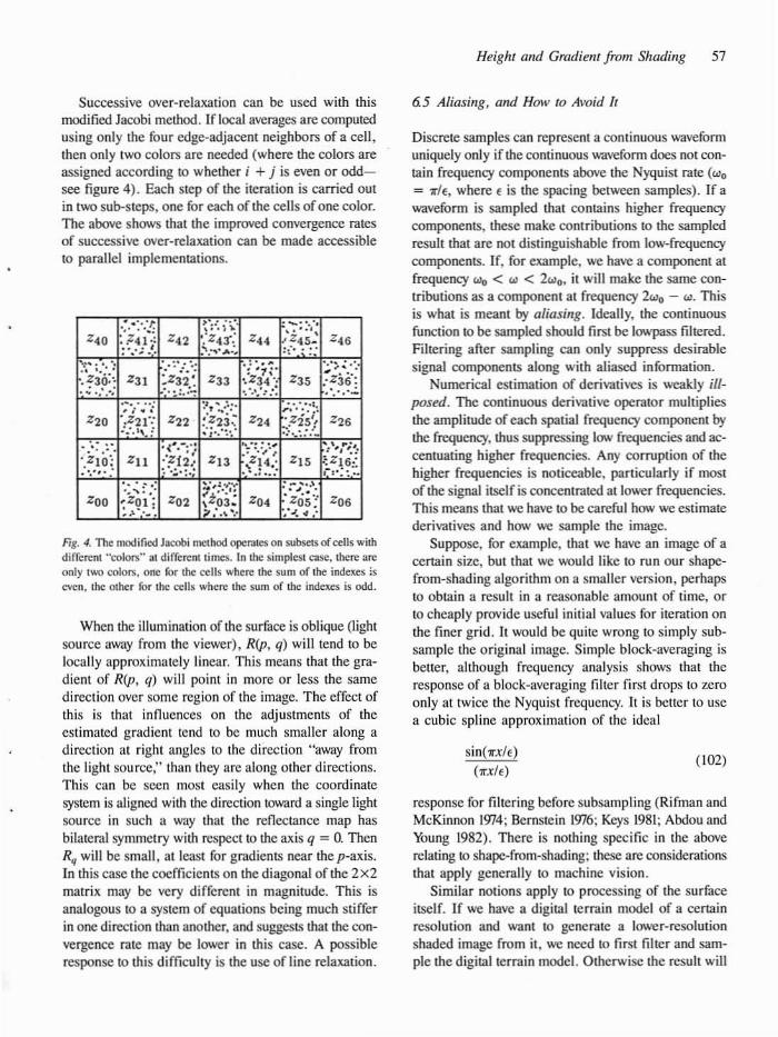
Rg. 4. The modirlCd Jaeobi ITIClhod operaleS on subsel$ofcclls wilhdifferent "eolors" al different limes. In thc simples! ClIse. thcre areonly two colon. onc IOr thc ccl1s where lhc sum or Ihc indexes ;seven. lhe other IOr llle alls where the sum or Ihe indc:xC$ is odd.

(102)sin(rxlt)(rxlt)

65 Aliasi"8. a"d HolV ro Amid Ir

response for filtering before subsampling (Rifman andMcKinnon 1974; Bernstein 1976; Keys 1981; Abdou andYoung 1982). There is nothing spccific in the aboverelating to shape-from-shading: thcse are considerationsthat apply generally 10 machine vision.

Similar nations apply to processing of the surfaceitself. If we have a digital terrain model of a certainresolution and want to generme a lower-resolutionshaded image from it, we need to firsl filler and sam­pie Ihe digital terrain model. Otherwisc the result will

Discrete sampies can represcnt a continuous wavefonnuniquely only if Ihe continuous wavefonn does not con­tain frequency components above Ihe Nyquist rale (wn= rh., where t is Ihe spacing bet'A-'Cen sampies). If awavefonn is sampled Ihat conlains higher frequencycomponents, Ihese make contributions to Ihe sampledresult Ihat are nol distinguishable from low-frequencycomponents. If, for eumple, we have a component atfrequency Wo < W < 2"'0' il will make the same con­tributions as a component at frequency 2"'0 - w. Thisis what is meant by aliasi/lg. Ideally. Ihe continuousfunclion to bc sampled should first be lowpass filtered.Filtering after sarnpling can only suppress desirablesignal components along with aliased information.

Numerical estimation of derivatives is weaL:ly i/I­posed. The continuous derivative operator multipliesIhe amplitude of each spatial frequency component bythe frequency, thus suppressing low frequencics and 3C­

centualing higher frequencies. Any corruption of thehigher frequencies is noticeable, parlicularly if mostof the signal itself is concentratcd atlower frequencies.This means that wc have to be careful how we estimatederivatives and how we sampie the image.

Suppose, for example. thai we have an image of aceTlain size, but that we YIOuld like 10 TUn our shape­from-shading algorithm on a smaller version, perhapsto obtain a result in a reasonable amount of time, orto cheaply provide useful initial values for ileration onthe finer grid. It would be quite wrong to simply sub­sampIe the original image. Simple block-averaging isbetter, although frequency analysis shows that Iheresponse of a block-averaging filter first drops to zeroonly at twice Ihe Nyquist frequency. It is beller to usea cubic spline approximation of the ideal

..'~~ .:4' ,'.

:~36 :, ....-

-:<.:-. .~".-;':

·.Z10: zl1 :~f2; Zu.',"': '. ':";.'

~- :::::.z30'·· z31......., .',

When the illumination of the surface is oblique (lightsource away from the viewcr), R(p, q) will tend to belocally approximately linear. This means that the gra­dient of R(p, q) will point in more or less the samedircction ovcr some region of the image. The effect ofthis is that innuences on the adjustments of thecstimated gradient tend to be much smaller along adireclion at righl angles 10 Ihe direction "away fromthe light source," than they are along other directions.This can be seen most easily when the coordinale~)'stem is aligncd with the direclion toWard a single lightsource in such a W'J.Y that Ihe reneclance map hasbilateral symmelry with respeCI to Ihc axis q = O. ThenRq will bc smalI, at leasl for gradients near the p-axis.In this casc the cocfficients on the diagonal oflhe 2x2malTix may be vcry different in magnitude. This isanalogous to a syslem of equations being much stifferin one direction Ihan another, and suggests that the con­vergence rate may bc lower in this case. A possibleresponse to this difficuhy is the usc of line relaxation.

Successive over-relaxalion can be used wilh IhisnxxIified Jacobi melhod. If !ocal averages are computedusing only Ihe four edge-adjacenl neighbors of a ceU,then only two colors are needed (where Ihe colors areassigned according to whether i + j is even or odd~see figure 4). Each step of Ihe iteration is carried outin lWO sub-sleps, one for each of Ihe cells of one color.The above shows Ihal the improved convergence ralesof successive over·relaxation can be made accessible10 parallel implemcnlations.

58 Hom

be subject 10 aliasing, and some fealUTeS of the shadedimage will not relate in a recognizable way 10 fealUresof the surface.

Finally, in creating synthetic dala it is not advisableto compute the surface gradient on a regular discreteset of points and then use the retloctance map tocalculate the expected brightness values. At the veryleast, one should perform this compulation on a gridthat is much finer than the final image, and then com­pute block averages of the result to simulate the effectof finite sensing element areas-just as is done in com­puter graphics to reduce aliasing effects.l6

(This hints at an interesting problem, by the way,since the brightness associated with the average sur­face orientation of a patch is typically not quite equalto the average brightness of the surface, since the reflec­tance map is not linear in the gradient. This means thatone has to use a retlectance map appropriate to theresolution one is working at-the reflectance mapdepends on the optical properties of the micrOSlrUclUreof the surface, and what is microstructure depends onat what scale one is viewing the surface.)

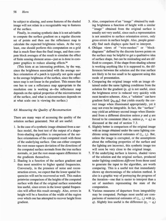
6:6 M~asuring the Quality of Reconstruct;on

There are many ways of accessing the quality of thesolution surface generated. Not all are useful:

I. In the caseofa synthetic imageobtained from a sur­face model, the best test of the output of a shape­from-shading a1gorithm is comparison of the sur­face orientations of the computed result with thoseof the underlying surface. One can either computethe root·mean-square deviation of the directions ofthe computed surface norrnals from the tnIe surfacenormals, or just the root-mean-square difference inthe gradients themselves.

2. Shading is a function of the surfaee gradient andthus most sensitive to higher spatial frequencies.Conversely. in the presenee of neise and recon­suuction errors, we expect !hat the lower spatial fre­quencies will not be recovered as weil. This makespointwise comparison of the heights ofthe computedsurface with that of the original surface somewhatless useful, since errors in the Iower spatiaI frequen­eies will affeet this result strongly. Also, errors inheight will be a funetion of the width of the regionover which one has atternpted 10 recover height fromgradient.

3. Also, comparison ofan "image" obtained by mak­ing brightness a function of height with a similar"image" obtained from the original surface isusually not very useful, since such a representationis not sensitive to surfaee orientation errors, onlygrass errors in surface heighl. Also, people gener­ally find such displays quite hard to interpret.

4. Oblique views of "wire-meshes" or "block­diagrams" defined by the discrete known points onthe surface may be helpful to get a qualitative ideaof surface shape, bot can be misleading and are dif­fieult to compare. If the shape·from-shading schemeis working anything like it is supposed to, the dif­ferenees between the solution and the true surfaeeare Iikely to be too small to be apparent using thismode of presentation.

5. Comparing the original image with an image ob­tained under the same lighting eonditions from thesolution for the gradient (p, q) is not useful, sincethe brightness error is redueed very quiekly withmost iterative schemes. Also, a "solution" can havegradient field {Ptt.qu} that yields exaetly the cor­rect image when iIIuminated appropriately, yet itmay not even be integrable. In fact, the "sunace"'may yield an arbitrary second image when illumin­ated from a different direction unless p and q areforced to be consistent (that iso unless Py = q.J asdiscussed at the end of section 7.3.

6. SlightJy better is comparison of the original imagewith an image obtained under the same lighting con­ditions using numerieal eslimales of (z..., zyl. But,unless the image is corrupted, or the assumptionsabout the refleeting properties of the surfaee andthe Iighting are incorrect, this synthetic image toowill soon be very e10se to the original image.

7. lf the underlying surfaee is known, shaded viewsof the solution and the original surfaee. producedunder lighling eonditions differellt from those usedto generate the input to the algorithm, are wonheomparing. This is a useful test that immediatelyshows up shoncomings of the solution method. ltalso is agraphie way of ponraying the progress ofthe iteration-one that is easier to interpret than aset of numbers representing the state of theeomputation.

8. Various measures of depanure from integrabilitymay be eomputed. Perhaps most useful are com­parisons of numerical estimates of (z.. , Zy) with (p,q). SlightJy less useful is the differenee (Py - q.J

(106)

(105)

of the solulion, since the heighl Z may still not haveconverged to the best fit to p and q, even when thegradient itself is almest integrable.

Q7 When 10 S10P Iterating

As is the case with many ilerative processes. it is dif­ficult to decide when to SIOP iteraling. Ifwe knew whatthe underlying surface was, we could just wait for thegradient of lhe solulion to approach that of the surface.But, other than when we lest the algorithm on synthericimages, we do not know what the surface is, otherwisewe would probably not be using a shape-from-shadingmethod in the first place! Some other test quantitiesindude:I. The brightness error

JJ(E(x, y) - R(p, q»' dx dy (103)

should be smalL Unfortunately this error becomessmall after just a few iterations, so it does nOI yielda useful stopping criterion.

2. A slightly different brightncss error measure

JJ(E(x, y) - R(zz, z,»l dz dy (104)

is a bit more useful, for while il approaches theabove when an exact solulion is obtained, it lagsbehind until the gradient of z equals (p, q). Whenan exaci solution is not possible, there will continue10 be small differences between the gradient ofzand(p, q), which means that this error measure doesnot tend to zero.

3. The departure from smoothness

JJ (Pi + p; + q; + q'j) dxdy

often drops as the solution is approached, but doesnot constitute a particularly good indicator of ap­proach to the solution. In particular, when onecomes dose to the solution, one may wish to reducethe parameter X. perhaps even 10 zero, in which casefurther iterations may actually reduce smoothnessin order to better satisfy the remaining criteria.

4. One of the measures of lack of integrability

Heigh, anti Gradient from Shading 59

is also not too useful, since it can al times becomesmalI, or stop changing significantly, even when zis slill inconsistenl with p and q.

5. Anotber measure of lack of integrability

JJ(zz - pp + (Z,. - q)2) d:c dy (101)

does appear to be very useful, since it drops slowlyand often keeps on changing unlil the iteration hasconverged.

6. One can also keep track of the rale of change of thesolution with iteralions

One should not stop until this has become smalI.In most cases it helps to continue for a while afterthe above measures stop changing rapidly since thesolution often continues to adjusl a bit.

Same of the implementation details given above mayappear to be extraneous. However, when all of thesemauers are anended to, then the iterative algorithm will

not "walk away" from the solution, and it will find thesolution, to machine precision, given exaCl data (andassuming that boundaJy condilions for p and q aregiven, and that h' is reduced to zero as the solutionis approached). Convergence to the exaCl solution willnot occur when something is amiss, such as a mismatehbetween the discrete estimatofS of the firsl derivativeand the discrete estimator of the Laplacian. It is notyet c1ear how significanl all of this is when one workswith real image data, where there is no exact solution,and where the error introduced by incorrect implemen­tation detail may be swamped by errors from othersources.

7 Some Experimental Results

The new algorithm has been applied to a number ofsynthetic images of simple shapes (such as an asym­metrica1 Gaussian, a sum ofGaussian blobs, and a sumof low-frequency sinusoidal gratings) generated with anumber of different refloctance maps (including onelinear in p and q, Lambertian with oblique illumina­tion, and a rotationally symmetrie one). These syntheticimages were small (usually 64x64 piClure cells) inorder to keep the computarional time manageable.Typica1ly the surface normals \W>uld be within a degree

60 Horn

or IWO of the oorrect direclion after a few hundred itera­lions. With appropriate boundary oonditions, the com~

puted shape would eventually be the same (10 machineprecison) as lhe shape used to generate the synthericimage. In each case, the brightness error decreasedmpidly, while the intcgmbility orthe cstimaled gradientdccrcased much more slowly.

7.1 Graphical Depicliorl 01 Solutioll Process

For help in debugging thc algorithm, and for purposesof detennining a good schedule for adjusting the

parameters I-t and >"', it is useful to print out thediagnostic measurernents discussed in sections 6.6 and6.7. But it is hard 10 tell exactly what is going on justby looking at a large table of numbers such as thatshown in figure 5. It is important 10 also provide somegraphie depiction of the CVQlving shape as it is corn­puted. 10 make shaded images orme rcconstructoo sur­face useful, however, they must be illuminated froma direction differem from the direction of illuminationused for thc original input image.37 Shown in figurc 6,is such a sequencc of shadcd images generatcd duringthe reconstruction of thc surlllce ofa polyhcdml object.staning from a random fjeld of surfacc oriemalions.

(...-Kho....I. 21l_, .. _ .... , •.•_ tr>., .._ ~1 __, .. _ ~l""·., I.'" e.,..._ •.nlIIt e.,..-. 1._ I~. M~I

I, , 1 Gr E, 2._" ...1.... E' '.5n", 1 -, E' •• _ n E' '._1 _th, 1.2_10 , • I:r E' I.~ "'1"" EI '.1"'" 1 -. E, 1.3111' U"" E' •..,.,,! -..., '."nI _,1."1_ ..,2.11:122110 , • llr E' '.27113 ...1..... h ' . .,m 1ft'" E' '.32'113 11....- E' '._.n ,-",-"", 1.1"" _,1.2922IllO ""'.s:l2~'l_: I."" "', '.1_ [P., .._ ~1"""", ..,_ ~I_ e--...., '.2stIt (:00-. 1._ I~ K ~I

I : i ........ E, '.213" E' '.13'" 1".-, E, •.1\l2t1 u EI ' ••nI2! _th, '.1620' _,.....", d.,.....35.10 : 2t;"ad E' '.2Im E' •. 13311 Ift'-' E' ....119 U E, '.'1"1) ..-th, •. nsn _,'."'952 do:'.12""n , N ....... E. '._1 1 E, '.1321' 1".-. E, '.1S4K U EI "" _th. '.n__".112I" .. , i1SOI , 32 Grad E, '.217e2 1 E' '.83~ 1ft'" E' '.158" U I, "'1 _th, '.115511 _" .•'2ll3 ... , 2215l_., •._ "', '.1_ b., .._ ~1""-"" 1._ ~I_., .._ C...- '.nlill c..-., I.IM" (,. M~'I

it : '0;"'" E, ......, ..I.... E' •.1:212 Ift'-' f, 0."2'25 11 I, '.121"' _ , '.1161" _".If2S13 ."'.111'"I, , '1 """" E' '.110" "I"', E' '.1:112 Ift'-' E' •.•_ Un' I, '.'21111 _ , '.0>119 _,'._122 ."'.IM1575it , 55 ~.d E, '.1133' ...."", E, '.12'" Ift'-' E' •.•~ {In.·•• (, '.'2"0 _th, 1.1"''' _,'.1_1 ."'.IM,"II , ,. c:r.d (, '.1122(, Or'''', E, '.12'" 1ft'" E, •••3552 (ln'-'. I, •••2177 """... , '.11>122 _".llilI'er.s ."'.lilIStMl_.. II.II~ "', '.111IIO E.., 1.lMlilI Al ....- ... ' 1.'1'1 ~1"".-.. 1.'_ c...-"., 1.2Sl10 Cor·, '.lIlil1' (,." "1Ito" 11II Ilr ... E, 11."611' ... IIIM E, 11.111523 1".-. E, '.'2'J3' (lft'-'. I' '.'2'6111 ....,.n ~' 11.11I152 "".,1.101535 ",,'.'11'"1it." % <:r.d (, 0.15"6 Orl.~. E, 1.115" 'n.·, E, '.1121101 (lft'-'. I, '.121'31 u...n ~, 1.118161 ••• ,1.111II32' ."'.11II21161I••" 112 ~r'" E, •• 16311 "'1..,. E, 1.11514 In'-' E, '.1I213i (1".-... E' '.1I213il u.. ,n, 1l,"1111 "".,1.11II1252 ",,'.112315I.." '28 Cr'" (, '.,il,5 .rl .... E, 11.'1513 In.-. E, '.1269' {lft.·.. I, •• 1121311 1Jft ~, '."111 "".,I.lilI'2" .".... '92.l_b<l., ••,," ""' ' ...IM h .. 1.(111II. AI"",- ... , I.JlII' A' ...._" LI'" c..--.. 1l.251ll C....-. l.lilIlll (i'·.6'1I.." ," ~oct E, '.14i55 1 , E, '.II.n In.-. f, 11.12'" U".-•• (, '.1211621 L>.- ~, '.19233 <IO.. ,Il._219 ......11511I , 192 c.- (, ,.,"11 1 E: 1l.1I'21 In.-. E: 1I.1215'l {lft.·.. I, •._1 ...., ,~, '.tt2'i _,'._1'2 ."'.11II1'"I , n. c.- (, '.1'252 .., E: ' ••1.21 'n._. E: 1.11:2'31 {ln.·.. E, '._21 ...., th: •.•~ _'Il....II••"'._1139, : 2'S6 E, '.1"39 .... ,..,. E: '.11121 , ...-. E: '.112121 Un.-... E' '.mo" ""'-"oth, '.'925' _:'._18' ."'._>3lricio: ' .•21. "", •• _ Ea>.: 1._ ~1""-",:",- ~l""_,, 1.1_ c..-...... l.nlIIt Cot"-..._ 160 M~I

h : 32'f Cro4 I' '.12422 ..I E: '._>3 1 -. E: ....n. (1ft..... h '.111931 """-,,, '.I(l4:M _,'._11' d _,.h : I, '.11'" ...1 f: '.ta,. 1 -. E: '.1132 (Ift'''''' E' '.111''' u..-u., '.11313 _:•• _ d 1III..13I : er E' '.iMI6 ..I f, '._3 1 -. E: '.1134' (In..... (, '.II<n1 u..-.., '.11'13 _,....n:JI d 126It : 512 g,-od I, '.i",2 ...1 f, '._1 1 -. I: ' .•11. (Ift'''''' I, '.II~" ,-",-", '.11"2 _:•._ ""21~".IIIM ... ' '.1SIlI l»o: .... ~l"""",,,_ 111 ....-0: I .... c..- I.:zsn c..--••._ 160 M 601..... : ... "'od I, •. _ I E, •. 10:3" 1 -. h ....16' <lft"_ I: ' .•13'.1 , •. 110&' _:•.__ ,•._~It.,., 1M ;,. I, •• _ 1 f, '.lIII316 1 -. I, '.'''53 11".- I, '.II:lt11 th: '.1151' _:•.~ d MtZSII : "' ;,. (, '.195" ..I f: •. 10:31' 1".-. E: ....'" (Ift h '.1131:21 : •. 1153' _" ...-n "','._1641 :112. ;,. I, •..,.." 1 I, ' ..an Ift'-' E, '.'U" (Ift'-'" I, '.II~I '-'"'-th, '.11551 _:•• _ .. "':'._111l-': •. teSt ..., &0: 1._ ~I""""": 1.'_ ~l""-t: 1.'- e--- '.2'SlII (:00-. 1._ (64 M 601it ,I211 ;"od I, '.lt2'9I 1 I, '.1I2ll2 , ....-. I, '.11591 11ft E, '.1I1Sl11 ....._tn, •. II~12 _,'.113722 d"'._33h :I536 ;,. 1:, •• I«J3t ..I E: '.1lIl2l1 In.-. E: •.11592 (In E, ......U lIno.-tn, '.1I61l1 _".113155 d"'._2'...... '1192 I, '.I~ 1 I, ••M2t1 1 -. E, •.01"' (Ift 8, •.••13111 ....._tn. '.lIi" _,•.1ln:XI1 d...._39h ... ,2041 ;"od E, '.1130' 1 I, '.M211 , -. E, '.115'1' (1".__ E, '.111391 _.~, '.11'" _,' .•83101 •• · ••1M.21Il_: •.Ili2f ... ' '.12IM E..: 1.'_ ~1""__: I .... ~I ....-" 1.'__ '.2SlII c..--••._. (64 K 601h :23.. ;"ocI E, '."'31 1 I, ' .•lIl1 , ....-. E' '.11341 (I".__ E, '.II51'! tn, •. 122.2 _,•.••152i ."'.1M1322it ,25611 Crocl i, 95 I E, ". I~.-. h '."331 (1ft.·.. E, ....511! _.~, 1.122" .""".IlI1:n, d"'.lilIl2I'1..,,2116 ;,.oct E, 932 1 E, ". In.-. E' '.'1336 UM-... I, 1.II55e! \lft ~, 1.I22i' ."'1.1112'1' ."'.!H1217...o,3Il~2 Cr.. E' ••11I92 1 < E, '.!HU' In.-. E, '.11336 \Ift'-Ild I:! 11.1155') ilft o.~, '.12261 ... '11.11'1216 ."'.lIIlIU3~_Od., ~.1lI11 ""' ' ••'I~ EoOl l.tl911 ~''''.-OQ' '.'ao~ A' ...._.' I."" e....-.. I.ZS" C....•• 1.11II1l (~" '"1•• ,,3321 ;,. •• I, ••~"" 11>-1..,. E, '.IIII"i In.-. E' '.11'3' (In.- I, 1.11619! ....,.ft.o,~, 1.12311 ... ,1.1115'3 ",,'.IIU9t1'.r,:I584 Cr•• E, '.UUi IritI>. E, 1.11I11I6 In'-. E, '.11'33 (IM- E, 1.lli19! 1Jn....o.~, 1.12381 "',I.III1'~' d"'.1t~3"

1••,,311', C,," 1:, •• 18865 IIrl .... E, 1.llll1i I~.·. E, '.11'33 (In.· I, 1.11611! \lft.ftoo'~' 1.1231U ,*.,1.11I'~3 d"'.1'239'I"",.,i ~r" E, I.I"~ 'rl,n. I, 11.11II1116 1"'-. E, '.11'33 U".- E, '.11'18! ""'• ....,.~, 1I.123U _,1.111092 .,,'.112'"~_"., 1l.'lilI5 "", '.1I1lHl EoOl 1.lllill\l AI ....- .... ' 1..1Il1 AI"".-" 1."11I Cot"-Ild 1l.~511 C....- ... lilIlIl (i'" ~I1 ,.3~2 c.- I, 1.l7i91 Orl,.". I, •._51 Ift,-, I, ••11111 Cln.- I, '.112901 ""' ~, 1.12155 _,•. lilIn2G d,,'.1M13961 '46.. c.- E, '.1762' "'1"'" E: •._., 1",-. E, '.''''1 (I".- E, '.I12tSJ _.~, '.1211'5 _".lilI1546 ."'.lilII3>11< ,"64 1:0' E, '.'15" ...1,.,,< E: '.llilI" 1".-. E, '.'''17 "".-.. I, '.11211'1 lJfto"'""~' '.121112 _,•. lilI~" ""'.lilII311i< :Sl2t ;"od E, •••1St. "'1..,. E, •._., 1",-. E, •.•111> Un..... I, '.112131 _.~: '.12fIS _,•. lilI7',. d"'.lilI'36'l_, •• _ "," '.lilI" E.o: I ..... 111 -0.' 1._ 111 .....-.' .. _ C....- ... '.nIM e....-. 1._ (,. K i411 :Sl16 llr E' ....., ..I E: •• _ , -....._ Cln h '.111261 _th, '.I32V _".tlIS2', d"'._331 :50i32 ;,. E' '.t66:t ...1 E, •. tlII3. 1ft'" EI ••_, 0 11 '.I1lnl _th: '.I~'" _,•.•"Uö3 d..'._"1t_,58IM ...ad E, '.tß99 ",_ E: •._ .".-, I' •._. C1n. __ E' '.111211 u.--th, '.13215 _'•.•"11' ."•._I .....:".. ;"ad E, ' ••5" ..I.... E: •• _ 1ft'" E, •• _ 11...• ... 11 ' .•'1211 ""-",,, '.132111 _'•.1""" dt:'._l-', '._2 "', •...,. Epo, .._ 1111_...,1.'- "'_,,, I.'" c..-... '.2'SfI c..--, 1._ (64 K i4)1 :6656 E, •. _ 1 E, '.MtZS 1".-. E, '._1 (1 - I, ' •..,.1 _th, '.13:1" _".8IS2lt2 ."•._1 :>1"" ;,. E: '.K:J9!I 1 E: '.tItZS 1ft'" E' ,.-' Cl • 11 '._1 l,Ino.nooth: '.I:J3t. _".tIS2>1 d,,'.__1 '_ I, '.1U9II "'1"'< I, '._n 1 -. E, ,.-' " h '._1 ....._th, '.I:J3t1 _,•. ttS26f ",,'._51t ,"52 llr E, '.1639' "'1..,. E: '._n 1 -. I, ...... IIn.· 11 •._1 _th, '.13312 _".ttS26f ""•.~~"._I "', '.M2t Ea>o: 1._ 111 , 1._ 111....-" 1._ e...-- '.2'SfI e-.• 1._ 16' M~)h ...,_ ;"ad E, ....,. 1 E: •. _ 1 - '.11112 IIn h •.•11621 _tn, '.131" _".lilI7>21 ""'.lilIl~

1"":'216 ;,..... i, ' .•955 , E, •. _ i -. h •.••012 Un h •.•"631 ..-th, '.13'12 _".lilI"" ""'.•1»51 ,"21 ;,... E' •.•'" 1 I, '._32 1 -... '.11112 CIn I, '."IU! _tn, '.13"1 _,'.lilI»« ""'.IMI",1 :..2.. ;,.... i' •.•'" e.-, E, •. _ 1 -. E, •.••1l12 U - E' ' .•nU)~, '.i3Ilil1 _'.....7•• d.....I53il_., •• _ "', ...... i •• , I.lilIlilI 111 ....- ' .. 111I 111 -" c..-__ '.2SIM C....•• 1._ 16< M i4)1t ,"152 Crod i' '.''''i7 e.-I E, '._1 1 -. E, '.lilIlll6 Uft E' '._92) _<.I" '.i6l93 _".'lilIII62 d IIII.'h ,I1U' ;,. I, '.1M"2 ...1 E, •. _ 1 -. E, '.lilI83' UM E' '.11M3I1 ....,......", •. 16:151 _,'._13 d _.2..... ,11'16 Cr E, '.lilI:Ji6 "I..,. E, '.11_ 1 -. EI 1.91111' U" E' •.••1.1 "",."""t./I, '.n"i ""'.e_5 d.. I.IIM.n1t... 112211 1:0'''' E' '.Nll' ""Oh' E, •.•_ 1".-. 11 '.lilIlIIl U".-o. I' •.•11I1» ....,."""'~, '.16.11 <10..1 ...11II13 d.... I1I11."

Fig. 5. Diagno~lic lniCe or vilrious error meilsurcs. This scquence of rcsulls corrcsponds 10 lhe rcconslruclion of lhe sharp-cdged enller shapcsllOWn in figurc 7. This kind or prcscnt.llion is il1lponunl. bUI mUSl bc supplememed by some graphie depiclion oflhe evolving solUlion surface.

Height and Gradiem from Shading 61

Fig. 6. Ream$lruclion or a porlion or a lruncatcd hcuhedron rrom a sh:tded image. Tbc dihedrnl angle: betwc:en c:ac:h pair ci lhe lhree Ol.Jlersurra.cc:s is 11:12. Tbis c:xample: illl.Jstrates thc: algoriltun'$ ability 10 dc:al ...-im surfac:c:s lhal~ !arge disconlinl.Jilic:s in surrace orielllalion.

Here the image provided 10 lhe algorithm conespondedto illumination from the northwcst, while illuminationfrom the northeast was uscd to display the reeonstrue­tion.lI Note how the edges beeome sharper as A', con­trolling the eontribution oflhe penalty term for depar­ture from smoothness, is made smaller and smaller.This example iIlustratcs the algorilhm's ability to dealwith surfuces that have discontinuities in surfaceorientation.

Becausc of thc inlCrest in application to astrogcology,aeraler-like shapc was also reconstruetcd, as shown infigure 7. In Ihis ease, thc algorithm rapidly found ashape Ihal was generally eorrect, exccpt for flaws inplaees on thc rim of Ihc eraler in the northeaSI andsouthwest. These are areas where there is liule con­trast bctween the inside and the outside of the craterin the input image.39 It took the algorithm a eonsiderablenumber of additional iterations to determine the correcteontinuation oflhe shapeeomputed in other imageareas.

7. 2 Emergem Global OrganilPtioll

Often progress toward the correct solution is not asuncventful. Frequently, small inlernally eonsistent solu­tion patchcs will establish themselves, with discontinu­ilics in surfaec orientalion where these patehes adjoin.Also, conical singularities form that tcnd 10 movc alongthe boundaries between such regions as thc iterativesolution progresses. Converscly, boundaries bctweensolution patehcs orten form along eurves connectingeonieal singularitics that fonn earlier. After a largecnough number of itcrations, patehes of local organiza­lion tcnd to eoalesce and lead to ell'lcrgent global organ­izallon. This ean be obscrved best when XI is smallerthan it would normally be for rapid eonvergenec. Infigures 8 and 9, for examplc, arc shown a scquencc ofshapes leading finally to a spherical cap on a planarsurfacc. Within some regions, solUlion surface palchesquiekly establish themselves that individually provide

62 Horn

Jt.-

Fig. 7. ReconSlruction of a cralcr-like shape. Points on lhe rim in lhe nonheaSl and lhe soulhwcsl correspond 10 places in lhe inpul imagewherc lherc is leasl eontras[ belwcen lhe inside and the outside. sinee the dircetion of lhe ineidenl illuminalion is paral1cllO the rim therc.

good matches to corresponding parts of the input image.The borders bctween these internally consistent regionsprovide error contributions that the algorithm slowlyrcduces by moving the boundaries and inerementallychanging the shapes within each of the regions. Toorapid a reduction of A' can remove the incentive to re­duce the creases and kinks and to freeze the solution inastate where some unnecessary discontinuities remain.If, for example, A' were to be set 10 zero with a "solu­tion" consisting of a spherical cap with an inner diskinverted, as in the right hand image of the middle rowoffigure 9, there would be no incentive to further reducethe length of the drcular discontinuity, and the smoothsolution for this part of the image would nol be found.

The algorithm was also applicd to impossible shadcdimages. Suppose, for example, that we are dcaling witha Lambertian surface illuminated by a source near theviewer and that there is a dark smudge in the middleof a large planar region racing us (whkh appears

brightly lit). It turns out that there is no surface withcontinuous first derivatives that could give rise to ashadcd image with a simply connected, bounded darkregion in the middle of a bright region (Horn, Szeliski,and Yuille 1989). In figure 10 we see what happenswhen the algorithm allempts 10 find a solution. Patchesgrow within which the solution is consistent with theimage, but there are discontinuities at boundaries bc­tween patches. Conical singularities sit astride theseboundaries. For all random initial conditions tried, thealgorithm evenrually eliminales all but one of these con­kai singularities. The computcd surface is in fact a"solution," if one is willing to allow such singularities.

The graphical method of presenting the progress ofthe iterative solutions illustratcd above was ver)' hclpfulin debugging the program and in determining reason­able schedules for reduction of the parameters A' andp.. Shown in figure 11 are some examples of what hap­pens when things go wrong. In the top row are shown

Height and Gradielll from Shading 63

Fig. 8. Emergenl global organizalion of local nonlinear iteralive proce's. Internally consislcm solution, arise in certain image patelIes witlldiscominuilie, at llle borden; belween regions. lhe boundaries !Jelween tllese palche, movc. and Ihe solulions wilhin lhe palclles adjust inorder 10 rcduce Ille ,um of the error terms.

instabilities arising in the solution for the craler-Iikeshape, near the points where there is low contrast be­tween the inside and the outside of the crater-that is,where there is no local evidence for curvature. Theseinstabilities can be suppressed by reducing A' moreslowly. In the middle row are shown patterns resultingfrom various programming errors. Final1y, in thebotlom row is shown the propagation of an instabilityfrom a free boundary when A' is set to zero. It appearsIhal the process is nOi stable without the regularizerwhen the boundary is completely free. This is not toosurprising, since the problem in this case may beunderdetennined.

In the past, shape-from-shading algorithms haveoften been "tested" by verifying that the computed gra­dient field actually generates something close to thegiven input image. To show jusl how dangerous thisis, consider figure 12, which demonstrates a ncw non­iterative method for recovering a "surface" given a

shaded image. In figure 12(a), is the input to (healgorithm, while figure 12(c) is what the gradient fieldthat is construeted by this algorithm looks like whenilluminated in the same way as the original surfaee.Figurc 12(b) shows wha( (he original surface looks likewhen il1uminated from another direction. As a test, weshould check whether the computed gradient field looksthe same under these illuminating eonditions. Butbehold, it does nOI! In Figure l2(d) we sec what weget when we use the other illuminating condition. The"trick" here is that the problem of shape from shadingis hcavily underconstrained if we are only eomputinga gradient field and not cnforcing integrability. Thereare many solutions and we can, in fact, impose addi­tional constraints. The underlying gradient field herewas computed by solving the photometrie stereo equa­tions (Woodham 1978, 1979, 1980a, 1989) for the twoimages in figures 12(c) and (d) under thc two assumedlighting eonditions.40

64 HOnJ

Fig. 9. Emergenl global organization of local nonlinear ileTalive proccss. Neighboring patehcs coaIcscc. as conical singularitics are absorbcdby coaIcscing wilh othcr singularitics. or by being pushc:d IOYo3rds a COlIIOIIr where the surracc oriclllalion is disconlinuous.. The final solutionis a sphcrical cap resling on a plane.

The new algorithm has also been applied 10 synthetieimages generated from more complicated surfaces suchas digital terrain models (DTMs) used earlier in re­search on interpretation of satellite images of hilly ter­rain (Horn and Bachman 1978; Sjobcrg and Horn 1983)and in automatie generation of shaded overlays fortopographie maps (Horn 1981). These synthetie imageswcre somewhat larger (the one used for figure 1 is ofsize 231XI78, for example). In this case, the simplealgorithm, presented in section 5.3, using a regulariz­ing term would often get trapped in a local minimumof the errar function after a small number of iterations,while the modified algorithm presented in section 5.6,exploiting the linearization of the reflectance map, wasable to proceed to a solution to machine precision aftera few thousand iterations. Most of the surface normalstypically were already within a degree or so ofthe cor­rect direction after a few hundred iterations.

The c10seness of approach to the true solution dependson several of the implementation details discussedearlier. In particular, it was helpfullo usc the old valuesof p and q for the reference point in the linearizationof R(p, q), rather than any of the other choices sug­gested earlier. Also, it helps 10 use the diagonal averag­ing scheme in lhe iteration for height rather than thescheme based on edge-adjacent neighbors.

7.3 Real Shaded lmnges

The new algorithm has also been applied to a few realimages, mostly aerial photographs and images takenby spacecraft. Shown here (figures 13 anti l4) are theresults obtained from a I08x128 palCh ofa 1024xl024SPOT satellite image (CNES-Central National Experi­mental Station, France) laken in 1988 oftbe HunlSVilIe,

Height alltl Gradient from Shading 65

Fig. Xl Whal happens ...·hen Ihc algorithm is confmnted ....ith an impossible shaded image? The input Image heTe (001 s/n'..n) is a circularl)'symmetlic dark smudgc in a unilOrml)' bright sunound. Thc light 5OUI'CC iSISliumed 10 be near the \·ie\I'('r. The algorilhm findsl ''Solution''....ith I single conical singularit)'.

Alabama region. The ground resolution of such images,that is, the spacing bctween piclure cells projected onthe surface, is 10 meters. The area of inlerest is MonteSano State P'drk. a lrce-covered hilly region east ofHuntsville.

The algorithm was run with frce boundary condi­tions on both height and gradient. With real data. thereIypically is no exact solution. and the error terms can­nOI bc reduced 10 zero. Correspondingly, wilh freeboundary conditions. Ihe iteralion is nOI stable whenthe regularizer is relllClYed completely, so thcre is a limiton how small onc can make "-'. Onc side-effect of thisis thaI the reconstrucled surface is somewhat smootherthan thc real surface and consequent.ly the vertical reliefis anenuated somewhat. The actual vertical reliefhere,for example, is about 250 m, while thc overall reliefin thc reconstruction is a bit less than 200 m.

At the time of this experimem, the viewing gcometryand the light sourcc position were not aV'dilable. norwas information on atmospheric conditions or sensorcalibration. The atJnospheric scattcr component wasestimated by looking in regions that appcar 10 bcshadowed, where Ihe reflected light cornponent is ex­pecled to be small (Woodham 198Ob: Horn and Sjoberg1983). The produci of illumination. surface albedo. andcamera sensitivity was estimated by looking in regionsthai appeared to be lumed to more or less face the lightsource. Unfortunately the range of grcy levels in theregion of interest was rather small (23-42), since thesensor had been adjusted so that it could cover the fulldynamic range nceded for the adjacent urban area.which was much brighler (21-149).·1 Also, comparisonofthe left and right images indicales that there may bea cerlain dcgrcc of aliasing in these images.

66 HOnl

Fig. /J. Graphical depiclion of inslllbilities and the cffocts of programming crrors. In lhe top row are shown inmbilitics I"Csulting from toompid rcduction of lhe penalty tenn for dcparluI"C from smoolhness. The middle row shows Ihc resuhs of various programming errors. Thebouorn row shows w.lVes of instability propagaling inwams frorn a fTee boundary.

The light souree elevation was estimated by assum­ing that the average brightness of the image was ap­proximately equal to the eosine of the angle betweenthe average loeal surfaee normal and the light soureedireetion. The polar angle of the light souree (90 0

minus the elevation aoove the horizon) can then befound if one assumes further that the average local sur­face nonnal is approximately vertical. For this image,this method yielded a polar angle of abaut 65~ or anelevation of 25 c:

The light souree azimuth, that is, the projection ofthe direetion toward the light source inta the imageplane, was first estimated to be abaut 60 0 c10ckwisefrom the x·axis of the image, based on the directionsof what appear to be shadows of tall buildings in thedowntow"n area ofHuntsVille, as weil as some other im­age features. Attempts to use Pentland's method(Pentland 1984) for estimation of the source azimuth

failed, as did Lee and Rosenfeld's refinement of thatmethod (Lee and Rosenfeld 1985). A reasonable diree­tion was found by instead eomputing the axis of leastinenia Ihrough the origin (Horn 1986) of a seattergramof the brightness gradient (Ex, E). There is a two wayambiguity in the result (eorresponding to the usual con­vex versus concave interpretations of a surface) that canbe resolved by other methods. Despite the emde natureof the scattergram, resulting from the coarse quantiza­tion of image irradiance measurements, an acceptableazimuth of betwcen 60 0 and 65 0 was found in thisfashion.

Finally, it was possible to refine this estimate oftheazimuth by running the shape from shading algorithmfor various source azimuths and recording the remain­ing solution errors after many iterations. There was abroad minimum near an azimuth of 65 c: This methodof estimating the source azimuth, while computationally

•

(.)

(c)

Height and Gradient from Shading 67

(b)

(d)

Fig. 12. Ncw onc-Slcp shapc-from-shading algorithm, See lexl!

expensive, scems 10 be relativcly reliablc, since theTedoes nOI appear to be a systematic deformation of thcsurface thai can compensate for a change in azimuthof the light SOUTee whilc yiclding a similar shadedimage. Unfortunately thc same cannat be said of theelevation angle of light souree position, since tilting thcsurface abau! an axis perpendicular 10 thc light SOUTeeposition, in such a way as to maintain thc angle be­twccn the average surface normal and thc direction 10the light SOU Tee, produces a similar shadcd image-atlcast 10 first order.

Shown in figure 13 is a regislcred stereo-pair ofSPOT images of thc Mante Sano Statc Park region.

NQle that Ihe Iighl comes from the lower fight (not the

upper left, as is common in artistic renderings ofsculpted surfaces). The stereo pair is shown here sothat the reader can gct a beller idea of Ihe aClUal sur­face shape. The algorithm, when presenled with theleft image of Ihe pair, ca1culates a shapc used 10 generateIhe synlhetic stereo pair in figure 14. (The vertical reliefhas been exaggerated slightly in the computation ofthesynthetic stereo pair in order to partially compcnsatefor Ihe attenuation of vertical relief mentioncd carlier.·Z)

Another way of presenling the resulling shape is asa contour map. Shown in Figure 15(a) is a portion ofthe USGS 7.5' quadrangle of the Huntsville Alabama

68 Rom

Fi,. /J. A stereo pair of SPOT salellile images of M()fIle Sano StaU: part: east of HUnl$Ville. Alabama. T1w: left subimage of tOS x 128 picturecells is used as input b' the dlape fmm sbiing a1gorilhm.

Ag. 14. A s)'nthetie stereo pair computed (rom the solution obtaincd by the ncw shape from shading algorithm.

area, with the area eovercd by the left satellitephotograph outlined, while figure 15(b) shows a eon­tour map derived from a smoothed form of Ihe solu­tion obtained by the shape-from-shading algorithm.This is not a comparison that is likely to be flalteringto the shape-from-shading algorithm, since we knowthat it is not very good at recovering the lower spatialfrequencies. Conversely, the shape-from-shadingalgorithm flnds a lot of detailed surface undulations thatcannot be represcnted in a contour map. For this reasonthe surface must bc smoothed or "generalized" beforecontours can be drJ.wn.

For want of a beller assumption, the spacecraft wasat first assumed to be vertically above the region of in­tercst when the image was taken. Judging from lateraldisplacements of surface features it appears. however,

that the left image was actually laken from a positionthat is about 15 0 aW'J.y from the nadir, in the directionof the negative x-axis of the image coordinate system(and the right image from a position roughly the sameamount in the other direclion). This means thai thecomputed result rcally applies to a tilted coordinatesystem. But more imponantiy, therc is a distonion intro­duced by a poor estimate ofthe source dircction occa­sioned by the assumption that average surface normalis parallel to the z-axis in the camera coordinate system.Anempts wcre made to compensate for this byeSlimating the source dircction based on the assump­tion that the average surface nonnal was tilted 15 0 inthe camera coordinate system. The TCConstroction pro­duced in this fashion was then rotated in Ihe .tZ-planeto bring it back into a1ignment with IDeal venical. While

Height and Gradient from Shading 69

Fig. /5. (alA portion of the USGS IOpographic map of thc: HURlSViI1c:, Alaharna area OOYering Montc: Saoo Stalc park, willltbc approximalearea OOYercd by thc Ieft salellilC image OUllined. The rcctanglc: is 3543' by 4200' (1080 m by 1280 m) and the ronIOur ißlcrval is 20' (6.1m). (b) ConlOUr mapdc:riYCd frum a smoot!Icd version ortbe solution oblained by thc shapc fmm shading a1gorithm from the Ic:fl salClIiIC imagc:.

lhe result produced in this way was better in certainways (lhe lateral displacement of terrain features wasgreatly reduced), it was worse in others (induding asmall till of the resull in the y direction). 1be moralis that 10 obrain quantiratively meaningful resuhs, Orteneeds 10 know aeeurately where the light source is inthe camera coordinate system-and, if the result is 10be relatcd to some external coordinate system, then thecamera position and attitude in that coordinate systemneeds to be known also.

The algorithm has, by the way, also been appliedto some images of Mars taken by the Viking Orbiter.Dut sinee the "ground truth" is not (yet) available inthe case of the Mars images, it is not possible to saymueh about the accuracy of the recovered surface orien­ration field.

7.4 Rating the Difficulty 0/ Shape-Jrom-ShadingProblems

Experiments with synthetic shaded images suggests thateertain shape·from-shading problems are relativelyeasy, while others are quite difficult. First oe all, basso­relievo surfaces (those with only low slopes) are easyto deal with (see also section 2.6) in comparison withalto-relievo surfaces (those with steep SIOpes).43 The

digital temlin model used for the experiment illustratedin figure I falls in the latter category, since the sidesoe the glacial cirque are steep and the individual gulliessteeper still.

1)tpically the brightness of a surfaee patch increasesthe more it is turned toward the light source. If it isturned too far, however, it becomes so steep that itsbrightrtess once again decreases. There is a qualitativedifference between shape-from-shading problems wherenone of the surface patches are tumed that far, and thosewhere some surface patches are so steep as to havereduced brightness. In the latter ease, there appears tobe a sorl of two-way ambiguity loeally abaut whethera pateh is dark beeause il has not been turned enoughto faee the light souree or whether it has been turned100 far. This ensures that simplistic schemes will gettrapped in local minima where patches of the solutionhave quite the wrong orientation. Similarly, the moresophisticated scheme described here tak.es many moreiterations to unkink. the resulting ereases.

The transition between the two situations dependson where the light source iso The difficulty is reducedwhen the illumination is oblique (see also section 2.6).Conversely, the problem is more severe when the lightsource is at the viewer, in which case brightnessdeereases with slope independent of the direction ofthe surface gradient. This explains why the algorithm

70 HOT/!

took longer to find the solulion in the case of thespherical cap (figure 8) since it was illuminated by asource near the viewer. It was more straightforv.'ard tofind the solutions for the truncated hexahedron and thecrnter-like surface (figures 6 and 7), both of which wereilluminated oblique1y. The above dichotomy is relatedto another factor: problems where the relevant pan oflhe reflectancc map is nearly linear in gradient are con­siderably easier to deal with than those in which thereflectance map displays strong curvatures of iso­brightness contours.

Smooth surfaces. panicularly when convex., can berccovered easily. Surfaces with rapid undulations andwrinkles, such as the digital terrain model surface(figure I) are harder. Discontinuities in surface orien­tation are even more difficult to deal with. Note that,with (he exception of the digitallerrain model, all oflhe examples givcn here in-.ulve surfaces that have somecurves along which the surface orientation is not con­tinuous. 1lle spherical cap. for example, lies on aplanarsurface, with a discontinuity in surface orientationwhere it touches the plane.

Problems where boundary conditions are notavailable, and where there are no occluding boundariesor singular poinl'l, are iIl posed, in the sense that aninfinite variety of surfaces could have given rise 10 theobserved shading. NOI 100 surprisingly these tend 10lead to instabilities in the algorithm, panicularly whenOlle auempts~to reduce the penalty term for departurefrom smoothness. In these eases instabilities ean bedamped out to some extent by enforcing the imageirradiance equation on the boundary by iterative ad­justment of the gradient eomputed from the discreteapproximalion of the natural boundary eonditions forfJ and q. But results have not been promising enoughto be worth discussing here in more detail.

Thc Ilumber ofitemtions to converge to a good solu­tion appears 10 grow almost quadratically with imagesire (number ofrows or eolumns). This is because someeffeets havc to "diffuse" across the image. This meansthat the tOlal amount of computation grows almost withIhe fourth power of the (linear) image size. It is weilknown lhal ordin.1ry iterative schemes for solving ellip­tic partial differential equations quickly damp OUIhigher spatial frequency errors, while low-frequencycomponents are removed vcry slowly. One way to dealwilh this problem is to use compUlation on coarser grids10 reduce the low spalial frequency components of Iheerror. This is the elassic Illultigrid approach (Brandt

Im?, 1980, 1984: Hackbush 1985: and Trottenberg1982). It is c1ear that a Irue multigrid implementation(as opposed to a simple pyramid scheme)44 would berequired to pursue this approach further on larger im­ages.·4This is mostly to cut down on the computationaleffort, bUI can also bc expccted to reduce even funherthe chance of geuing caughl in a loeal minimum oftheerrar function. Implemcnlaüon, hCM"CVer. is ll()( trivial.since the equations are nonlinear. and because thereare boundary conditions. 80lh of these factors com­plicate malters. and il is known thai poor implementa­tion can greatly reduce thc favorable con"ergence rateof the hask multigrid schcme (Brandt ICJ1? 1980. 1984).

Altematively. one may wish 10 apply so-callcd direclmethods for solving Poisson's equations (Simchony.Chellappa, and Shao 1989).

8 Conclusion

The original approach to the general shape-from­shading problem requircs numerical solUlion of IhecharacleriSlic strip equations Ihal arise from thc first­order nonlincar panial differential equmion Ihat rdatesimage irradiance to scene irradiance (Horn 1970. ImS).\arialional approachcs 10 the problem inslead minimizethe sum of Ihe brightness error and a penalty term suchas a measure of depanure from smoothness. Theseyield second-order partial diffcrenlial equalions whosediscrete approximation on a regular grid can be con­veniently solved by classic ilerative techniques fromnumerical analysis. Several ofthese lllcthods, however.compute surface orientation, not heighl. ;md do nOl en­sure that lhe resulting gradient field is integrable(Ikeuchi and Horn 1981: Brooks lind Horn 1985). OneIhus has, as a second slep. 10 find a surface whose gra­dient comcs elosest to lhe estimated gradient field ina least~squarcs sense (see Ikeuchi 1984: Horn 1986. eh.11; Horn und Brooks 1986).

The two stcps can be combincd. and lhe accuracyofthe estin13ted surface shape improved considcrably.by alternately taking one step of the ileration forrccovering surfacc orientation from brightness. and Ollestcp of the iteration that recovers the surface that beSIfits Ihe current estim;lle of thc surface gradient. Thisidea can be formalized by setting Up::l vari3tiorul prob­lem involving both the surfacc height above a refercnceplane and Ihe first pani::ll derivmives thcrcof. The

•

resulting set of three coupled Euler equations can bediscretized and 5OlvOO much as lhe two coupled equa­lions are in the simpler methods thai recover only SUT­face orientalion.

Such an itcr,lIive scheme for recovering shape fromshading has been implemented. The new schemerecovers height and gradient at the same time.Linearization of lhe reflectance map abau! the localaverage surface orientation greatly improves the per­formance of the new algorithm and could be used toimprove the performance of existing iterative shape­from-shading algorithms. The new algorithm has beensuccessfully applied to complex wrinkJed surfaces, evensurfaces with discontinuitics in the gradient.

9 Acknowledgements

This article describes research dooe in part al the Arti­ficiallnlelligence Laboratory of the Massachusetts In­stitute ofTechnology. Support for the laboralory's ar­tificial intclligence research is provided in part by theAdvanccd Research ProjeclS Agen<.)' ofthe Dcpartmentof Defensc under Office of Naval Research contractNOOOI4-85-K-0124.

Michael Caplinger kindly provided pointers to rele­vant publicalions on photoclinometry, in particular thePh.D. thesis of R.L. Kirk at the Califomia Institute ofTechnology. Michael Brooks drew my attention to thefact that clCisting iterative schemes "walk away" fromthe correct solUlion and that regulariution does not"pick one of thc infinite number of solutions" of anill-posed problem, as is sometimes mistakenly stated.Bradford Washburn supplicd a detailcd IOpographicmap of the Mt. Washington area of the White Moun­tains in New Hampshire from which digital terrainm<Xiels used in the experiments here were interpolated.Steve Ahlmer and Michael Caplinger provided realshaded images of terrain on Earth and on Mars. JoelMoses found a way for the Electrical Engineering andComputer Science Depanmem to help cover the costofthe author's trave!to the photoclinometry workshopheld al Arizona State University, Fcbruary 12-13, 1989,This workshop provided much of the impetus for thework rcportcd here. Michael Brooks, Eric Grimson,and Tcrcsa Ehling provided additional helpfulcommenlS.

Heighl and GrruJienr from Shading 71

Notes

I. A gradient field is integrable ir il is Ihe grndienl or some sur­race height runction.

2. The gullies are sleep enough to Ix: or interest 10 ice c1imbcrs.3. For additional examples or reeonslructions rrom shaded images.

sec seclion 7.4. In lhe uample:$lrial. Ihe a1gorithm a1ways reroverallhe under­

Iying surf:ace orientation exaetly al every pietuce cell. staningfrom a random surface orkntlllion rlCld, providal!hal boundar)'information was available. Sinct: lhe queslion ofu.niqueness ofsotutions !las TJOIlx:en lOIaI.Iy resoIved. one cannot Ix: quite cauinthallhere may llOI be c:ases ....here. differenl soIulion mighl befoond !hal nappens 10 also fil lhe given image dala exaetly.

5. In phoIocIinomelT)' il is CUSIOmaT)' to use an objed..:erllCral C(l()r­

dinale sySiern. This is because surface shapc can bc compuledatong profiles only ....hen strong additional conslraint is provided,and such eonslrainlS arc bcSI expressed in an obje~1-eemercd

coordinate syslem. Working in an objccl-centered coordinalesystem. ho....ever. makcs the fonnulalion or the sl1ape-from·shading problem considerably mon: compln (sec, ror eum­pie. (Rindneb<:h 1966»).

6. Grey-Ievels are quanlized e:$linwes of image irradianee.7. Tbc:[number is lhe ratio of the principaI diSlaIlCC 10 lhe di.lmeltt

of the apcnuI"C. !hal is_ fld.8. Dip is Ihe angle belwcen a given surfaa: and the lJoriwnuI p13l1l: •

....l1ile 51rike is the direclion of the inlerseetion of the surfaceand the horUonlat plane. Tbc: line ofinlersection is pcrpcndieular10 lhe direction or sleepesl descent.

9. Luminancc longilude and lalitude are the longitude and Inlitudeor a poim on n sphere with lhe givcn orienlalion. llleasured inaspherkaI coordinale sySlem .... ilh lhe poles al righl angles 10boIh the direclion lo....ard the souree and lhe direetion lo....ardlhe vie...-er.

10. Incidence and emiuance ;lnglc:s are rneaningful quaJ1l:ilie:$ onl)'when there is a single source; and tVen lhen there is. lwo-.....y.mbiguily in surfilee orienlalion unless addilional informationis providal. 1lIc: same applies to luminalK% Jongiludc: andlalilUde.

11. Tbc:re is a small problem. ho....ever.....ilh lhis rnethod ror spcei­rying thc direclion lo....ard the lighl source: A souree may bc"behind" thc scene. wilh thc dircclion 10 the souree more Ihnn'/(/2 away from lhe dircclion towllrd thc vicwer. In chis ClIse thez-<:omponenl of lhe veclor poinling IOward Ihe Iighl souree isnegative.

12. Tbc coordillllics of gradicm SfNJet are p and q, Ihe slopes ofthe surf:ace in lhe.l and y direclion respcelively.

13. NOIe!ha1 shape·from--shOlding melhods ace mOSI definilely n(}l

rcsuiCied 10 Larnbenian surfaca. Soch spcci;aJ surfaca rnm:lyprovide • convenienl pcdagOSica1 device for i1Ilß1Taling Roiic_.

14. Ifthere is a uniquc: muimum in ref1«1ed brighlnC:SS. iI is 00fl·

venienllo rcscale Ihe measuremeIW so lhallhis eXlremum cor­responds 10 E • I. The same npplies whcn thcre is a uniqueminimum, as is lhe case for the 5Canning eleclTon mieroscopc(SEM).

15. We see thaI C : s • P. : q,. so lhnl Ihe direclion spceified inIhe image by (c, s) is lhe direetion .. to....ard lhe !IOUrce:' thaiis, the projeclion inlo Ihe image plane or Ihc vttlor i towan!lhe lighl souree.

72 Horn

16. Iflhe funelionJis not monotonie, there will be more titan onesolution fOT eertain briglttness values, In this case one llUty needto introduce assumptions about conlinuity of Iltc derivatives inorder to decide wlticlt solution to cltoose.

17. Tlte integnltion is, of COUlOe, earried out numerically. since Ilteintegrand is derivcd from image measurcments and notrcpresenled as an analylic funetion.

18. l1Je reneetance map is rotationally symmetrie, for example. whenIltc source is where the viewer iso OT wlten an extended sourceis symmetrieally distributed aboul the dircction lOw.lTd the viewer.

19. Methods for reeOliering tlte shapes of polyhedral objects usingsltading on the faees and tlte direetions ofthe projections ofllteedges into the image arc diseusscd in (Sugihara 1986) anti (Horn1986).

20. Tlte same argument applies when tlte unique exlremum is aminimum, as il is in tlte case of scanning electron microseope(SEM) illUtges.

21. The shape-from·shading problem ean be formulated and soh-edwlten Ilte viewer and tlte lighl sourecs are not at a grcal distanee(Rindfleisch 1966; Horn 1910, 1975), but then scene radiancedepends on posilion as weil as surfaee orientalion, and tlte na­tion of a renectance map is not direelly applieable.

22. A gradient·field (or ncedle diagmm) (P(X. y). q(x, y)} is integrableiftherc exists some surface Iteighl funetion z(x, y) such Ihatp(x,y) = z~(x, y) and q(x, y) = z,.(x, y), where tlte subscriplS denolCpartial derivatives.

23. Genenllly. a small patclt of a shaded image is infinilely am­biguous. Also. without integrability, Ihe problem of recoveringa gnldient field is generaHy ill posed. But ifwe impose integrabil­ily, and provide suitable boundary conditions, then Ihe sltape­from-shading problem is definitely /lQ/ i1l posed (Bruss 1982;Deift and Sylvesler 1981; Bmoks 1983; Blake. Zisserman. andKnowlcs 1985; Saxberg 1988).

24. Note that ..... here is /l0f a Lagrange multiplier, bUI a faelor thatbalanees the relative contributions of the brightness error termanti the ICI"QI measuring departure from SmootllIlCSS. Tl1:lt iso thereis no absolute commim imposed here. only a penalty term addedIhat inereases willt departure from smoothncss.

25. Tltere are several methods for approximating tlte Laplacianoperator, including five-point and nine-point approximations. ltis weil known Iltal. wltilc the nine-point approximalion involvcsmorc computation. ilS lowest-order error term Itas a Itigher orderIltan that of the five-point approximation (Horn 1986).

26. Herc K = 4 whcn Ihe local avernge AI is computed using thefour cdge-adjacent neighbors. wltile K = 1013. when 1/5 of theavernse of the corner-adjaeent nciShbolO is addcd 10 4/5 of theaverdge of the cdge-adjaeem neigltbors (see also scelion 6.2).

'll. These cquations are solved iterntively blxause the system of cqua­lions is so large and becausc oflhe factlltat Ilte reflectance mapR(p, q) is typically nonlinear.

28. The rcsuhing gradienl field is likely not to be integrable becausewc have not enforeed the eondilion P, = q~. whielt correspondsto Zxy = Zw

29. Natural boundary conditions arise in variational problems wltereno boundary eonditions are explicitly imposed (Courant andHilbert 1953).

30. The referenee gradient will, of course, be differenl at every pie­ture eell. but to avoid having subscript~ on the subscripts. wcwill simply denote the reference grddient at a partieular pieturecell by (Po. qo).

31. l1Je new shape-from-shading algorithm. of course. workscquallyweil on synthetie shaded images of digital temlin models ob­taincd by other means. such as onc ofthe Les Diablerets regionsof Switzerland used in (Horn and Bachman 1978).

32. See (Lee 1988) for a pmof of convergence or an iterative shape­from-shading sclteme.

33. The ··red" and "blaek" squares are the eells fOT which Ilte sumof the row and column indexes arc evcn an<! odd respeetively.

34. It may appear that this difficulty sterns from the use of s\aggeredgrids. The problem is even m)rse when aligncd grids are used.however. because the discretc cstimator of the Laplacian con­sistent with simple cenlnll differenee eSlimators oflhe first par­tial derivalives has a support that includes only ceHs that are 2faway from Ihe center. And this form of the Laplacian openltoris known to be badly behavcd. We find that there are Jour de­coupled subsets of cells in Ihis case.

35. Conversely. if Ilte basie melhod ltas a tendency to be unstable.Ihen one can ··under·relax':....that is, Ust a value IX < I.

36. One can obtain good symhetie data. however, wilh an exaetalgebraie solution, by sampling Ihe heigltt on a regular discrcteseI ofpoints and then cstimating the deriV"dlives numerieally. asdiscussed in scetion 5.1. This was done here to generate mostof the e~mple5 shown in section 7.

n. The leSt illumination should be quite different from the illumina­lion used to genernte Ihe original image-preferrably lying ina direelion tltat differs front the original sourcc direction by asmuch as 'lrf2.

38. The input image is not shown. but is just like the last image inIlte scquenee shown. exeept Ihal left and right arc reverse<!.

39. Again, the inpul image is not shown. but is lik.e the last imagein the scquence sltown. e~cepl thatleft and righl are reverse<!.

40. There is no guarantce Ihalthere is a solution oflhe photometriestereo problem fOT surfaee orientation, gi\'en tm) arbitrarybrightness values. since Ilte two cquations are nonlinear. In thepartieular ease shown here. the dynamie nlnge of the Im) im­ages was suelt Ihm a solution could be found al all bUI aboula huntlrcd picturc eells.

41. The mapping finally cltosen took a grey level of22 into 0.0 anda grey level of 43 into 1.0 nomJalized surface radiance.

42. While the basc-to-height ralio in the satellite images appears 10

be about 0.5. il was assumcd 10 be 0.75 for purposes oflhe com­putation of the synthetic slereo pair.

43. For more regarding lhe lerms basso-reliel'O, t1Jez;p-reliel'O andaflo-reliel'O (see Koenderink. and van Doorn 1980).

44. A naive approach has one solve the cqualions on a coarse gridfirst. with the results used as inilial conditions for a finer gridsolution after inlerpolation. True multigrid methods are morecomple~. bUI also have much better propcrties.

10 References

I.E. AlxIou and K.Y. Wong, ·"Analysis oflincar interpolation schemcsFor bilevel image appliealions," IBM J. Res. Del"elop.26(6):667-686. 1982 (see appendix).

R. Bernstein, "Digital intage proeessins of earth observation sensordata." IBM J. Res. !JeI·t!/op. 20(1):40-57, 1976 (see appendi~).

•

A. Blake. A. Zissmnan. ard G. Knowles. -Surface Oesaiptiom fl'OOlSleROand shadi~,- I~ V"uiof'l CcmpuL 3(4):183-191. 1985. Abo

in Horn arid BlOOb. 1989.WJ. Bonncr and R.A. Schmal!. ':A pbotomeuic teehniquc for deter­

mining planelary slopes fmm orbital phoIograplls;' U.s. GmlogicalSurvcy ProfC$sional P:lpcr 812-A. pp. 1-16, 1973.

A. Br.mdt, "Multi-level adaptive solutions 10 boundary-Ylllue pro!>­lems." Malh~rtUlfics of CompufOliOll 31(138):333-390. 1977.

A. Brandt. "Stages in developing multigrid solutions:' In E. Absi,R. Glowinski. P. Laseaux, aod H. VeysseyTe (ed$.), NunwrirnJM~thods for Engin«ring. Dunod: Paris. pp. 23-44. 1980.

A. Br.llldt. "Muhigrid ICChniquCS: 1984 guide with applialtions 10fluid dynamia." mooqraph a--ailable as GMD-Swdie No. &S. fromGMD-FIT, f'o5Ifach 1240. D-25OS, St. Augustin I. Wesl Gennany.19ß4.

A. Brandt and N. Dinar, "Mulligrid solutions of clliplic now prob­lems:' In S.V. f'Jrter (ed.), NumerirnJ MI'/hcdsfor PDE. AcadrnticPress: Ncw York, 1979.

M.l. Bmoks. "1Wo rcsults concerning ambiguity in shape from,hading," Proc. Nat. Con! Arti! InitII. • pp. 36-39. Wa!;hington.D.C., August 22-26, 1983.

MJ. Brooks, pel$Onal communiauion. 1985.M.l Brooks and B.K.P. Horn. "SIIapc and SO\IfCC from shading,"

Prot:. InI~rn. Joint Conf Anif. Iflttll., pp. 932-936, Lo5 AlJ8eles.AugllSl 18-23. t985.. Also in Horn and Brooks. 1989.

A.R. BTUSS. '1'he Ekonal cquation: Somc rcsuIlS applialble 10 com­plItef vision:' J. Ph)'Sics 23(5):890-896, t982. Also in Horn andBrooks, 1989.

R. COUr1tnl and D. Hilben. Melhods ofMmhematical Ph)'Sics. vol.I. Wiley: New York, 1953.

R. Coumnl and D. Hilben, Melhods o[MlI/hemaliC/iI Physks. \"01.

11. Wilcy: New York. 1962.P.A. Davis. and A.S. MeEwcn, "PlIoloclinomclry: AlI:llysis of in­

hcrent elTOBand implicalions lOr IOpograpbic mcasuremenl," 15fh/.MnDrandPlafltItllySdmaCOt(. pp. J94-195. ~1arch 12-16.1934.

P.A. Davis and 1..A. SodcrbIom. "Rapid alnClion of relath~

qJOgr.Iphy from VLking Orbiter~: U. Appl.icalion 10 intguIar\OpOgraphic falures," fkporu Off P/tJneIDry GeolotY Progrom,

NASA Tcchnical Memorandum 86246, pp. 29-JO. t983.P.A. Davis and L.A. Soderblom, "Modcling craler l(Ipogl3phy and

albedo from rnonosoopic Viking OrbilCr irnages: I. Melhodology:'J. Geoph)'S. Ru. 89(BII):9449*9457, 1984.

P,A. Davis. L.A. Soderblom, and E.M. Eliason. "Rapid cslinullionof Manian topogmphy from Viking Orbiler image phOIOmClry:'&pons QfI P/(,mCf{2r)' Gcology Progrom, NASA TechnicalMcmorandum 85127, pp. 331-332, 1982.

P. Dcift and J. Sylvester. "Somc remarks on thc shapc-from-slt3dingproblem in compulCr vision." J. MrMh. Anal. Appl. 84(1):235-24&.1981-

R.T. FnnkoI and R. Chdbppa. "A mcthod lOr cnlOrcin& inIqI2bililyin shape from shading algorilhms," IEEE TmJIS.. Paltern Anal.Mach. l/1/ell. 10(4):439-451. 198& Also in Horn and Brooks. 1989.

P.R. Garabcdian, Panial DifJ~~fltial€qua/ions. Wiley: New "Ort,1964.

W. Hackbush, Mlilligrid Me/Iw<is mul Applications. Springcr·Verlag:Berlin, 1985.

W. Haekbu.'lh. and U. Trollenberg (cds,), Mulrigrid M~/hods. Springcr·Verlag: Berlin, 1982.

Height alld Gradienl from Shading 73

B.W. Hap«. "A lheoreIical pholOmeuic funetion for thc lUllölr sur­racc:' J. GropIryJ. Res. 68(15):4571-4586. 1963.

B.W. Hapke, "An improYCd lhcoretlca\ h/llölr pbolOmctric function."Asfrrmomical Journal 71(5):333-339. 1965.

B'w. Hapkc, "Bidireclional rcllectancc speclroscopy: (I) Thcory:'J. G~oph)'s, Res. 86(84):3039-3054, 1981.

B'w. Hapke, "Bidlrcclional rellcclance SpcclTOSCOPY: (3) Corrcclionfor macroscopic roughncss." lrorus 59:41-59. 1984.

B.W. Hapke and E. \\klls, "Bidirectional rd1ec1allCC spcctroscopy:(2) Experirnentl .nd obscTVllllions:' J. G~oph)'s. Res.86(84):3055-3060. 1981.

J.G. Harns. 'Thc0JUpla:i dcplhIsiope approach 10 surfacc~tion.R 5.101. lbesh. DepanrncntoiElearical En~andCom­plIlCr SciCIICC. MIT, 1986. Also Tedutiall Rcpon 908. Artilici:l1InlClligcncc Laboral(lry, MIT, Cambrldgc. MA, t986.

10. HaITis.. "A ncw approadi 10 surfacc reconslrtlC1ion: ThccouplcddeptlJlslope model." Proc. Imern. Con! CampUf. Vision. pp.277-283, London, Junc 8-1l, 1987.

B.K.P. Horn. "Sh:lpc from shading: A melhod for obtaining lhc shapeof a smooth opaquc object from onc view." Ph.D. Thesis. Ocpan­rnentofElcetrical Engineering, MIT. Im Also Technical RcportTR·I9, Pro;ccl MAC. MIT, Cambridgc. MA. Also Teclmical RcportTR·232. AnirlCialllllClligcnce Labor.wory, MIT. Cambridge. MA.lm

B.K.P. Horn. "Obcaining shape from shading inlOrmation:' In P.H.WillSlOD (cd.). The P$ydto/ogyofComp"'~~ V"uian. Mc:Qr:IW Hili:New "Ort.. Im, PP- 115-155. Also in Horn and Brooks, 1989.

B.K.P. Horn. "UndcßWlding image intensilics (sie):' Anifida/l/1/el·Iigence 8(2):201*231, lW7. Also in M.A. FischleT and Q Firschcin(eds.). Readings in Computer VisiQIl. pp. 45-60, Kaufmann: Los

Allas, CA. 1987.B.K,P. Horn. "Hili shading and lhe rellcclancc map," Proc. IEEE

69(1):14-47, 1981. Also in Geo-Processing 2(1):65-146, 1982, aod''AUtomallc hill-shading and thc rellect:lIlce map:' I~ Unde~·

SkIIIding KfH'bhop, pp. 19-120. Palo Aho. CA. April 24-25. 19i1IJ.B.K.P. Horn. "E:uended Gaussian images:' Proc. IEEE

72(12):)611-1686,. 1984.B.K.P. Horn, Rabol V"uion. MIT Press: Cambridgc. MA; and

McGraw-Hill: New York. 1986.B.K.P. Horn. "Parallel analog ncl\lo()rl:s b machinc vision:' rnemo

1071, Anificial Inlelllgcnce laboratory, MIT, Cambridgc, MA,Dcccmbcr 1988.

B.K.P. Horn and B.L. Bachman, "Using ~)'mhetic images la n:gislcrreal images wilh surfacc models," Commullictui/JIts ofl!t~ ACM21(11):914-924, 1978. Also "Rcgistering real images using synlheticimages." In P.H. Wirr;lOIl. and R.H. Brown (ros.). Anijiciallllltl·ligence: All Mrr Ptrs:p«tivr. vol. 11. pp. 129·)6Q, MIT Press: Cam­bridge, MA, 1'178.

B.K.P. Horn and MJ. Brooks. "Tbc variational approach 10 shapefrom shading," Compttl. Vision, Graph. Ima~ Prouss.33(2):174-208, 1986. Also in Horn and Brooks. 1989.

B.K.P. Horn and M.J. Brool:s (ros.), ShDpefrom $hading. MIT Press:Cambridge, MA, 1989.

B.K.P. Horn and B.o. Schunck. "DclCnnining optical fkrw." Anijidallmelligence 17(3):185-203. 1981. Also Memo 572. AnifieiallnlCl·lillenee Laboralory. MIT. Cambrid8c, MA, April 1980.

B.K.P. Horn, and R'w. Sjobcrg, "Calculatin8lhe rcllectance map,"Applied Oplks. 18(1I):17iU-1179. Junc 1979. Also in Horn andBrool:s, 1989.

74 Horn

RK.P. Horn, R. Szeliski, and A.L. YiJille, "Impossible shadedimages," submiucd to IEEE Trans. PAMT, 1989.

A.D. Howard, K.R. Blasius, and .lA. Cun, "Photoclinometrie deter­mination ofthe topogrnphy ofthe Martian North Polar Cap," Icarw50:2455-258, 1982.

K. Ikeuehi, "Rcconstrueting a dcpth map from intensity maps," Intern.Gonf Paltern Recog. pp. 736-738, Montreal, July 3O--August2, 1984.Also "Construeting a depth map from images," Memo 744, Anifi­ciallntelligence Lahoratory, MIT, Cambridge, MA, August 1983.

K. lkeuchi and B.K.P. Horn, "Numerical shape from shading andoccluding houndaries," Anificial Tmelligence 17(3):141-184, 1981.Also in Horn and Brooks, 1989.

F. John, Par/ial Differeruial EiJuarions. Springer-Verlag: Berlin, 1978.R.G. Keys, "Cubic eonvolution interpolation for digital image pro­

cessing:' IEEE Trans. Acoust., Speech Signal Process.29(6):1153-1l60, 1981.

R.L. Kirk, ''A finite-element approach to two-dimensionalphotoclinometry:' Abstract in 8ull. Amer: krronom. Soc. 16(3):Xl9,1984.

R.L. Kirk, ''A fast finite-element algorithm for two·dimensionalphotoclinometry:' Part m ofPh.D. Thesis, Division ofGeologiealand Planetary Sciences, California Institute of Technology,Pasadena, CA, 1987.

JJ. Kocnderink and A.J. van Doorn, "Photometrie invariants relatedto solid shape:' Oprica Acta 27(7):981-996, 1980. Also in Hornand Brooks, 1989.

J.J. Lambiotlf: and G.R. Taylor, ''A photometrie technique for derivingslopes from lunar orbiter photography," Proc. Conf Use ofSpuceSyslemJfor Planetary Geology und Geophysics, Boston, MA, May25-27, 1967.

C-H. Lee and A. Roscnfeld, "Improved methods of estimating shapefrom shading using the light source coordinate system" AnifieialIntelligence 26(2):125-143, 1985. Also in Horn and Bmoks, 1989.

D. Lee, ''Algorithms for shape from shading and occluding houn­daries," Proc. IEEE Conf COmpUI. Vision Palrem Recog. , pp.478-485, Ann ArOOr, MI, June 5-9, 198& Also in Horn and Brooks,1989.

B.K. Lucchitta and N.A. Gamhell, "Evaluation of photoclioometricprofile determination." In Analysis ofApollo 8 Pholographs andVisual Observalions, NASA SP-201, National Aeronauties andSpaee Administration, pp. 51-59, 1970.

J. Malik aod D. Maydan, "Rccovering three dimensional shape froma ~ingle image ofeurved objects," IEEE Trans, l'I;J.lfem Anal. Mach.Imell. 11(6):555-566, 1989. Also in Horn and Bmoks, 1989.

M.C Malin and G.E. Danielson, "Topography on Ganymede derivedfrom photoclinometry" Repons on Planetary Geology Program,NASA Technical Memorandum 86246, pp, 29-30, 1983.

A.S. MeEwen, "Thpography and albedo ofIus Chasma, Mars," 16thLunar and Pwnetary Sei. Conf pp. 528-529, March 11-15, 1985.

E, Mingolla and lT. Todd (1986), Perception of solid shape fromshading:' Biological Cybernelic$ 53:137-151. Also in Horn andBrooks, 1989.

M. Minnacrt, "Photometry of the moon:' In G.P. Kuiper and B.M.Middlehurst (eds.), PIaneis and Solelliles: The Solar Syslem, vol.3, eh. 6, pp, 213-248, University ofChicago Press: Chicago, 1961.

Q.R. Passey aod E.M. Shoemaker, "Craters and baslns on Ganymedeaod Cal1isto: Morphologieal indicators of erustal evolution:' In D.Morrison, (cd,), Salel/iles ofJupirer, pp. 379-434, University ofArizona Press: Tueson, 1982.

A.P. Pcntland, "Local shading analysis," IEEE Trans. POllern Allo/.Mach. Inlell. 6(2):170-!87, 1984. Also in Horn and Brooks. 1989.

A.P. Pentland. "Shape information from shading: A thcory ahouthuman perception," Teehnical Repon 103, Vision Sciences, MITMedia Laboratory, MIT, Cambridge. MA. May 1988.

S.S. Rifman aod D.M. MeKinnon, "Evaluation ofdigit.al correctionteehniques-for ERTS images," Repon Number E74-10792, TRWSystems Group, July, 1974 (see eh. 4). Also Final Repon TRW20634-6003-TU.QO. NASA Goddard Spaee Flight Center.

T. Rindfleisch, "Photometrie method for lunar topog"~phy,"

Phorogrammetric Engineering 32(2):262-277, March 1966. Also''A photometrie method for deriving lunar topographie informa­tion," Technieal Report 32-786, Jet Propulsion Laboratory, Califor­nia Institute of Technology, Pasadena, CA, September 1965.

L.C Rowan, J.F. MeCaulcy and E.A. Holm, "Lunar terrain map­ping and relative roughness analysis," U.S. Geological Survcy Pro­fessional Paper 599-G, pp. 1-32, 1971.

RV.H. Saxherg, ''A modem differential geometrie approach to shapefrom shading," Ph.D. Thesis, Department of Electrieal Engineer­ing and Computer Science, MIT, Cambridge. MA, 1988.

M. Shao, T. Simehony, and R. Chellappa, "Ncw algorithms forreconstruction of a 3-D depth map from 01lC of more images:' Proc.IEEE Con[ Compur, Vision Poltern Recog. Ann "rhor. MI, June5-9, pp. 530-535, 1988.

T. Simchony, R. Chellappa, and M. Shao, "Direct analytical methodsfOT solving Poisson equations in computer vision problems:'Published report, University of Southcm Califomia, 1989. Alsoin IEEE GompUl. Soc. "brl:slwp on Compur. Visiml. Miami Beach,FL, November 1989.

R.W. Sjoherg and RK.P. Horn, "Atmospherie effeets in satellite im­

aging of mountainous terrain," Applied Oprics 22(11):1702-1716.1983,

S.W. Squyres, "The topography of Ganymede's grooved terrain,"lcarus 46:156-168, 1981.

T. Strat. ''A numerical method for shape from shading for a singleimage:' SM Thesis, Depanmcnt of Elertrical Engineering andComputer Stienee, MIT, Cambridge, MA, 1979.

K. Sugihara, Machine Inrerprerarion ofUne Drawings, MIT Press:Cambridge, MA, ch. 10, 1986.

D. Terropoulos, "Multilcvel eomput.ational processes for visual sur­face reconstruetion," Compul. Vision. Graph. Image Process.24:52-96, 1983. Also "Multi-level reconstruction of visual sur­faces: variational prineiples and finite element representation,"Memo 671, Anificial Intelligcnce Laboratory, MIT, Cambridge,MA, April 1982.

D. Terropoulos, "Multigrid relaxation methods and the analysis ofHghtness, shading, and flow," Memo 803, Anificial lntelligenceLahoratory, MIT, Cambridge, MA, October 1984. Also in S.Ullman and W. Richards (eds.), Image Undersranding 84. AblexPublishing Corporation: NoTWJOd, NJ, eh. 10, pp. 225-262, 1984.

G.L. Tyler, R,A. Simpson. and HJ. Moore. "Lunar slope distribu­tions: Comparison of bi-st.atie radar and photographie rcsults:' J.Geophys. Res. 76(11):2790-2795, 1971.

K. Watson, "Photoclinometry from spacecral\ images:' U.S.Geologieal Survey Professional Paper 599·B, pp. 1-10, 1968­

R.L. Wildey, "Gcneralizcd photoclinometry for Mariner 9," Icarus25:613-626, 1975.

R,L. Wildey, "Topography from single radar images," Science,224:153-156, April 1984.

•

R.L. Wilde)', "Radarclioometry for Ihe Venus radar mapper;'f'holotIram.. Enginur.~Sms. :52(1):41-SQ 1986. Also in Hornand Brooks. 1989.

D.E. Wilhehll$, "A pbokJmetric tecltnqiue br measuremml cf lunarslopc:s:' Astrogeologirol 511uJirs AwI.IolJI Progrrss &port. Pon D:Srwiicsfvr Spoa f1iglu Program. U.S. Geolosical Survey Open­File Report. pp. 1-12. NASA Calalog Number N66 3:5:597. Mzy_.

L. Wilson. M.A. Brown. E.M. Pannenlier. and J.W. Head...Theoretical lI5pects cf pholoclioomelry Ierrain plOriling on tbeGalilean saleUites:' Ikpons on l'ttJMl(lry CNokJgy Progrom. NASATedmical Memorandum 86246, pp. 27-28. 1983.

L. Wilson. 15. HlIßlplOO. and H.C. Baien. "PholOclioometry cf 1eT­

resInai and p1anettry surraces:' 16th UutiJr and i"IlJM/lJry Sd. Confpp. 912-913, March 11-15, 198:5.

R.J. Woodham. "A cooperalivc algorilhm for delcrmining surfaceoricntllliun from a single Yiew," lilie"'. Joiflt COflf. Anif. lmell.,pp. 63:5-641. Cambridge, MA, August 22-2:5, 1977.

Height and Gmdiem lro", Shadillg 75

RJ. Woodham. "Photometrie stereo: A renec\atlC<:: map ItChniquebr determinil1fl surfaa: orientalion fTOm a single vicvo·... Proc.. Soc.PhoIo-Oprirot IllSrrumcu. &gin. 15:5:136-143. Im.

RJ. \l.bodham. '~nalyzing curved surface5 using reIlectance mapleChniques:' In P.H. WiIlSlOll and R.H. Brown (eds.). AnificioJl~tligC'ltU: An MfT hrsp«lilT (Voh,une 11). MIT Press: Cam­bridge. MA. "llI. U. pp. KiI-I84. 1979.

RJ. \\\:Iodham...Phoklmctric method brdelenninina sulfxe orien­talion flOm mulliple images." OplictJ1 Enginuring 19(1):139-144.198Oa. Also in Horn and Brooks. 1989.

RJ. \l.bodham. "Using Iernin digilal dala 10 model Image bma­lion in remole sensing," lmilgC' Pro«u. G"itlßnu, SPIE238:361-369. 198Ob.

R.1 Woodham. "Determining surface curvalure wilh pholomeuicslereo:' Proc. tEEE Canf. lWborics AuIQmlJl.• May 14-19. 1989.