169

Tampereen teknillinen yliopisto. Julkaisu 853 Tampere University of Technology. Publication 853 Heikki Hurskainen Research Tools and Architectural Considerations for Future GNSS Receivers Thesis for the degree of Doctor of Technology to be presented with due permission for public examination and criticism in Tietotalo Building, Auditorium TB111, at Tampere University of Technology, on the 7th of December 2009, at 12 noon. Tampereen teknillinen yliopisto - Tampere University of Technology Tampere 2009
ISBN 978-952-15-2270-3 (printed) ISBN 978-952-15-2291-8 (PDF) ISSN 1459-2045


ABSTRACT
Satellite navigation has emerged to be one of our every-day technologies, like wi-reless communication. The U.S. based Global Positioning System, better known asGPS, was the first system to serve civilian users. Today, GPS is under moderniza-tion, Europe has devoted a lot of effort to build their own system, called Galileo, andactivities around Russian GLONASS system are also being re-initiated.
The users benefit of having multiple systems with more satellites available. This canbe made possible by the receiver, which should be able to process the new modula-tions and frequencies introduced in modern navigation signals. This thesis is aboutreceivers for future Global Navigation Satellite System (GNSS). Especially the fo-cus is on baseband issues of a combined GPS and Galileo receiver, with exploitingtheir similar Code Division Multiple Access (CDMA) signal structure and sharedfrequency bands.
The work presented in this thesis deals with the tools for research and developmentof such a receivers, and outlines the potential future receiver architectures. For theresearch community the biggest advantage in receiver simulators would be having astandardized research environment, enabling the fair comparison of the results fromdifferent studies, e.g. in the area of multipath mitigation.
The Software Defined Radio (SDR) has been discussed in context on GNSS recei-vers before, in this thesis an overview of the current situation is given with discus-sion on hardware and software trade-offs. Hardware engines are still dominating incommercial receivers, but more flexible SDR architectures are emerging in researchtools. Last, a novel approach of using a multicore processing platform architecturefor GNSS receiver implementation is presented. This approach is seen to have agreat potential in future receivers, especially since it could also be used to realizeother technologies, like wireless communication, in the same device.

ii Abstract
PREFACE
The work presented in this thesis has been carried out in the Department of ComputerSystems at Tampere University of Technology during the years 2005-2009.
I would like to thank my supervisor Professor Jari Nurmi for the given opportunity todo this work and also for his ”Freedom for all and feedback on demand” approach.I would also like thank Dr.Tech. Heidi Kuusniemi and Ph.D. Fadio Dovis for theirefforts in reviewing this thesis.
I give my special thanks to Jussi Raasakka for his comments on (and off) topic, toDocent Elena-Simona Lohan for sharing her ideas and knowledge, and to all co-authors of the enclosed publications for their contribution. At last I want to thankall members of Team Nurmi, especially the ones actively joining the 2 PM coffeebreaks, for creating a pleasant and inspiring atmosphere for working.
The research work was funded by Department of Computer Systems, European Unionand Finnish Funding Agency for Technology and Innovation (TEKES) projects. Thisthesis was financially supported by Tuula and Yrjo Neuvo Foundation, Finnish Foun-dation for Technology Promotion (TES), and Ulla Tuominen Foundation which isgratefully acknowledged.
Finally, family and friends, thank you for your support and everything else. I dedicatethis thesis to my children Aapo and Helka.
Tampere, December 2009
Heikki Hurskainen

iv Preface

TABLE OF CONTENTS
Abstract . . . . . . . . . . . . . . . . . . . . . . . . . . . . . . . . . . . . i
Preface . . . . . . . . . . . . . . . . . . . . . . . . . . . . . . . . . . . . . iii
Table of Contents . . . . . . . . . . . . . . . . . . . . . . . . . . . . . . . v
List of Publications . . . . . . . . . . . . . . . . . . . . . . . . . . . . . . ix
List of Figures . . . . . . . . . . . . . . . . . . . . . . . . . . . . . . . . . xi
List of Tables . . . . . . . . . . . . . . . . . . . . . . . . . . . . . . . . . xiii
List of Abbreviations . . . . . . . . . . . . . . . . . . . . . . . . . . . . . . xv
List of Symbols . . . . . . . . . . . . . . . . . . . . . . . . . . . . . . . . xxi
1. Introduction . . . . . . . . . . . . . . . . . . . . . . . . . . . . . . . . 1
1.1 Scope of the thesis . . . . . . . . . . . . . . . . . . . . . . . . . . 2
1.2 Thesis organization . . . . . . . . . . . . . . . . . . . . . . . . . . 3
2. Satellite Navigation . . . . . . . . . . . . . . . . . . . . . . . . . . . . 5
2.1 Fundamentals for satellite positioning . . . . . . . . . . . . . . . . 5
2.2 Global Satellite Navigation Systems . . . . . . . . . . . . . . . . . 6
2.2.1 GPS . . . . . . . . . . . . . . . . . . . . . . . . . . . . . . 6
2.2.2 GLONASS . . . . . . . . . . . . . . . . . . . . . . . . . . 7
2.2.3 Galileo . . . . . . . . . . . . . . . . . . . . . . . . . . . . 9
2.2.4 Other sources for satellite navigation . . . . . . . . . . . . 10
2.3 Users of GNSS application . . . . . . . . . . . . . . . . . . . . . . 10
2.3.1 Use cases for GNSS . . . . . . . . . . . . . . . . . . . . . 10

vi Table of Contents
2.3.2 GNSS industry and markets . . . . . . . . . . . . . . . . . 11
3. GNSS signals and receiver fundamentals . . . . . . . . . . . . . . . . . . 13
3.1 Reception of navigation signals . . . . . . . . . . . . . . . . . . . . 13
3.1.1 Navigation frequencies . . . . . . . . . . . . . . . . . . . . 13
3.1.2 Antenna . . . . . . . . . . . . . . . . . . . . . . . . . . . . 14
3.1.3 Radio-frequency stage . . . . . . . . . . . . . . . . . . . . 14
3.2 Finding the satellites . . . . . . . . . . . . . . . . . . . . . . . . . 16
3.2.1 Ranging codes . . . . . . . . . . . . . . . . . . . . . . . . 17
3.2.2 Modulation techniques . . . . . . . . . . . . . . . . . . . . 22
3.2.3 Autocorrelation function . . . . . . . . . . . . . . . . . . . 23
3.2.4 Acquisition . . . . . . . . . . . . . . . . . . . . . . . . . . 24
3.3 Measuring pseudoranges . . . . . . . . . . . . . . . . . . . . . . . 26
3.3.1 Measurement breakdown . . . . . . . . . . . . . . . . . . . 26
3.3.2 Tracking . . . . . . . . . . . . . . . . . . . . . . . . . . . 28
3.4 Estimating the position . . . . . . . . . . . . . . . . . . . . . . . . 34
4. GNSS receiver tools . . . . . . . . . . . . . . . . . . . . . . . . . . . . 37
4.1 Link level tools . . . . . . . . . . . . . . . . . . . . . . . . . . . . 37
4.1.1 GRANADA . . . . . . . . . . . . . . . . . . . . . . . . . . 37
4.1.2 SMOG . . . . . . . . . . . . . . . . . . . . . . . . . . . . 39
4.2 Multi-channel simulators . . . . . . . . . . . . . . . . . . . . . . . 39
4.2.1 DGC SDR GPS . . . . . . . . . . . . . . . . . . . . . . . . 39
4.2.2 Namuru Receiver . . . . . . . . . . . . . . . . . . . . . . . 40
4.2.3 NavX-NSR . . . . . . . . . . . . . . . . . . . . . . . . . . 40
4.2.4 N-Gene . . . . . . . . . . . . . . . . . . . . . . . . . . . . 42
4.2.5 GNSS Receiver Reference Design - TUTGNSS . . . . . . . 42
4.2.6 C++ TUTGNSS . . . . . . . . . . . . . . . . . . . . . . . 42
Table of Contents vii
5. Architectural considerations for GNSS receivers . . . . . . . . . . . . . . 45
5.1 Common design requirements for embedded receivers . . . . . . . . 45
5.1.1 Processing power . . . . . . . . . . . . . . . . . . . . . . . 45
5.1.2 Memory . . . . . . . . . . . . . . . . . . . . . . . . . . . . 45
5.1.3 Power consumption . . . . . . . . . . . . . . . . . . . . . . 46
5.1.4 Cost . . . . . . . . . . . . . . . . . . . . . . . . . . . . . . 46
5.2 Overview of receiver architectures . . . . . . . . . . . . . . . . . . 46
5.2.1 State-of-the-art GNSS receivers . . . . . . . . . . . . . . . 47
5.2.2 Towards SDR . . . . . . . . . . . . . . . . . . . . . . . . . 48
5.2.3 GNSS acceleration with flexible tracking channels . . . . . 50
5.2.4 SDR with multiple cores . . . . . . . . . . . . . . . . . . . 52
6. Summary of Publications . . . . . . . . . . . . . . . . . . . . . . . . . 55
6.1 General . . . . . . . . . . . . . . . . . . . . . . . . . . . . . . . . 55
6.2 Overview of the publication results . . . . . . . . . . . . . . . . . . 55
6.3 Author’s contribution to publications . . . . . . . . . . . . . . . . . 56
7. Conclusions . . . . . . . . . . . . . . . . . . . . . . . . . . . . . . . . 59
7.1 Main Results . . . . . . . . . . . . . . . . . . . . . . . . . . . . . 59
7.2 Future Trends . . . . . . . . . . . . . . . . . . . . . . . . . . . . . 60
Bibliography . . . . . . . . . . . . . . . . . . . . . . . . . . . . . . . . . . 63

viii Table of Contents
LIST OF PUBLICATIONS
This thesis is based on the work published in scientific conferences and journalsduring 2006–2009. These publications are listed below and enclosed in the part twoof the thesis. In text, these publications are referred to as [P1], ... ,[P7].
[P1] Heikki Hurskainen, and Jari Nurmi, “SystemC Model of an InteroperativeGPS/Galileo Code Correlator Channel”, in Proceedings of the IEEE Work-shop on Signal Processing Systems Design and Implementation (SIPS). Banff,Canada, October 2–4, 2006, pp. 348–353.
[P2] Heikki Hurskainen, Xuan Hu, Sireesha Ancha, Graham Bell, Jussi Raasakka,and Jari Nurmi. “Enhancing Usability of the GRANADA Bit-True ReceiverSimulation on Galileo L1”, in Proceedings of the 20th International Techni-cal Meeting of the Satellite Division of the Institute of Navigation ION GNSS2007. Fort Worth, TX, September 25–28, 2007, pp. 2707–2714.
[P3] Heikki Hurskainen, Elena-Simona Lohan, Xuan Hu, Jussi Raasakka, andJari Nurmi, “Multiple Gate Delay Tracking Structures for GNSS Signals andTheir Evaluation with Simulink, SystemC and VHDL”, International Jour-nal of Navigation and Observation, vol. 2008, Article ID 785695, 17 pages,2008. doi:10.1155/2008/785695.
[P4] Heikki Hurskainen, Tommi Paakki, Zhongqi Liu, Jussi Raasakka, and JariNurmi “GNSS Receiver Reference Design”, in Proceedings of 4th AdvancedSatellite Mobile Systems (ASMS) conference 2008. Bologna, Italy, August26–28, 2008, pp. 204–209.
[P5] Heikki Hurskainen, Jussi Raasakka, and Jari Nurmi “Specification of GNSSApplication for Multiprocessor Platform”, in Proceedings of InternationalSymposium on System-on-Chip (SOC) 2008. Tampere, Finland, November4–6, 2008, pp. 128–133.

x List of Publications
[P6] Heikki Hurskainen, Jussi Raasakka, Tapani Ahonen, and Jari Nurmi. “Mul-ticore Software Defined Radio Architecture for GNSS Receiver Signal Pro-cessing”, EURASIP Journal on Embedded Systems, vol. 2009, Article ID543720, 10 pages, 2009. doi:10.1155/2009/543720.
[P7] Heikki Hurskainen, Elena-Simona Lohan, Jari Nurmi, Stephan Sand, Chris-tian Mensing, and Marco Detratti. “Optimal Dual Frequency Combinationfor Galileo Mass Market Receiver Baseband”, in Proceedings of the IEEEWorkshop on Signal Processing Systems Design and Implementation (SIPS).Tampere, Finland, October 7–9, 2009, pp. 261–266.

LIST OF FIGURES
1 GPS Selective Availability . . . . . . . . . . . . . . . . . . . . . . 8
2 GPS and Galileo signals . . . . . . . . . . . . . . . . . . . . . . . 14
3 Radio . . . . . . . . . . . . . . . . . . . . . . . . . . . . . . . . . 15
4 GPS C/A code generator . . . . . . . . . . . . . . . . . . . . . . . 19
5 GPS L5 code generator . . . . . . . . . . . . . . . . . . . . . . . . 20
6 Galileo E5 code generator . . . . . . . . . . . . . . . . . . . . . . 21
7 ACFs for Galileo . . . . . . . . . . . . . . . . . . . . . . . . . . . 24
8 FFT Acquisition . . . . . . . . . . . . . . . . . . . . . . . . . . . . 26
9 GNSS signal modulation and demodulation . . . . . . . . . . . . . 28
10 GNSS tracking channel . . . . . . . . . . . . . . . . . . . . . . . . 29
11 Constructive and destructive multipaths . . . . . . . . . . . . . . . 32
12 Simple MGD . . . . . . . . . . . . . . . . . . . . . . . . . . . . . 33
13 Multipath Error Envelopes . . . . . . . . . . . . . . . . . . . . . . 34
14 GRANADA bit-true simulator . . . . . . . . . . . . . . . . . . . . 38
15 Namuru V2 . . . . . . . . . . . . . . . . . . . . . . . . . . . . . . 41
16 Cost vs. MIPS in GPS receiver . . . . . . . . . . . . . . . . . . . . 49
17 Input multiplexer . . . . . . . . . . . . . . . . . . . . . . . . . . . 50
18 Flexible tracking channel . . . . . . . . . . . . . . . . . . . . . . . 51
19 Multicore SDR GNSS . . . . . . . . . . . . . . . . . . . . . . . . . 53

xii List of Figures

LIST OF TABLES
1 GNSS RF front ends . . . . . . . . . . . . . . . . . . . . . . . . . 16
2 XOR function . . . . . . . . . . . . . . . . . . . . . . . . . . . . . 17
3 GPS and Galileo signals . . . . . . . . . . . . . . . . . . . . . . . 25

xiv List of Tables

LIST OF ABBREVIATIONS
ADC Analog to Digital Converter
API Application Programming Interface
ASIC Application Specific Integrated Circuit
BCU Baseband Converter Unit
BOM Bill-Of-Material
BW Bandwidth
C/A Coarse/Acquisition
CDMA Code Division Multiple Access
CL (GPS L2C) Long Code
CM (GPS L2C) Moderate length Code
CPU Central Processing Unit
CRISP Cutting edge Reconfigurable IC’s for Stream Processing
CS Commercial Service
DC Direct Current
DGC Danish GPS Center
DLL Delay Locked Loop
DS Direct Sequence
DSP Digital Signal Processor

xvi List of Abbreviations
DVD Digital Versatile Disc
E Early (correlator)
EC European Commission
EGNOS European Geostationary Navigation Overlay Service
EML Early Minus Late
ESA European Space Agency
EU European Union
FCM Factored Correlator Model
FFT Fast Fourier Transform
FLL Frequency Locked Loop
FOC Full Operational Capability
FP Frame Programme
FPGA Field Programmable Gate Array
GARDA GAlileo Receiver Development Activities
GIOVE Galileo In-Orbit Validation Element
GLONASS GLObal’naya NAvigatsionnaya Sputnikovaya Sistema
GNSS Global Navigation Satellite System
GP I/O General Purpose Input/Output
GPP General Purpose Processor
GPS NAVSTAR Global Positioning System
GRAMMAR Galileo Ready Advanced Mass MArket Receiver
GRANADA Galileo Receiver ANAlysis and Design Application
GREAT Galileo REceivers for mAss markeT

xvii
GSA European GNSS Supervisory Authority
GSM Global System for Mobile communications
HPGPS High Performance GPS
HRC High Resolution Correlator
IC Integrated Circuit
IEEE Institute of Electrical and Electronics Engineers
IF Intermediate Frequency
IFFT Inverse FFT
IMU Inertial Measurement Unit
IOC Initial Operational Capability
ION Institute of Navigation
IOV In-Orbit Validation
IP Intellectual Property
ITU International Telecommunications Union
L Late (correlator)
L2C GPS L2 Civil signal
LFSR Linear Feedback Shift Register
LNA Low Noise Amplifier
LO Local Oscillator
LoS Line-of-Sight
MEE Multipath Error Envelope
MEO Medium Earth Orbit
MGD Multiple Gate Delay

xviii List of Abbreviations
MIPS Million Instructions Per Second
MM Multipath Mitigation
MUX MUltipleXer
NavSAS Navigation Signal Analysis and Simulation
NCO Numerically Controlled Oscillator
NEML Narrow EML
LoS Non-Line-of-Sight
NoC Network-on-Chip
NRE NonRecurring Engineering
OS Open Service
P Prompt (correlator)
PC Personal Computer
PLL Phase Locked Loop
PND Personal Navigation Device
PPS Precise Positioning Service
PRS Public Regulated Service
PSD Power Spectral Density
PVT Position, Velocity and Time
QZSS Quasi-Zenith Satellite System
R&D Research and Development
RF Radio Frequency
RHCP Right Hand Circular Polarization
RS232 Recommended Standard 232 (serial port)

xix
SA Selective Availability
SBAS Satellite Based Augmentation System
SDR Software Defined Radio
SDRAM Synchronous Dynamic Random Access Memory
SMOG Simulink Model Of Galileo
SoL Safety-of-Life
SPS Standard Positioning Service
SRAM Static Random Access Memory
SS Spread Spectrum
TUT Tampere University of Technology
UNSW University of New South Wales
USB Universal Serial Bus
VE very-early (correlator)
VHDL VHSIC Hardware Description Language
VHSIC Very High Speed IC
VL very-late (correlator)
VLIW Very Long Instruction Word
WAAS Wide Area Augmentation System
WCDMA Wideband CDMA
XOR eXclusive-OR

xx List of Abbreviations

LIST OF SYMBOLS
a weighting factor (MGD)
bu receiver clock bias
c constant of the speed of light (299,792,458 m/s)
∆t signal travelling time
fc frequency of the PRN code
fIF frequency of the IF
fs frequency of the subcarrier
fsignal frequency of the received signal
fLO frequency of the local oscillator
Hz Hertz (unit of frequency)
ρ pseudorange
ρi pseudorange from user to satellite i
W Watt (unit of power)
(xi,yi,zi) location coordinates of satellite i
(xu,yu,zu) location coordinates of the user

xxii List of Symbols

1. INTRODUCTION
In the early 1990’s quite few people had a phone in their car. After a bit more thana decade, a person without a personal (mobile) phone is more exceptional than onewith a phone. The same thing is now happening to satellite navigation receivers. Inthe early 2000’s the car navigators started to enter to the markets, and now in the endof the very same decade quite many people are trusting their on-road navigation tosatellites. Besides cars, the satellite navigation has also entered to pedestrian level,where it is usually integrated with communication technology into the same device.
American Global Positioning System (GPS) was the first one to offer global satel-lite positioning. It is been followed by Russian GLONASS and European Galileosystems. By mid-2010’s there will be more satellites for navigation in the sky thanever. New systems and the modernization program of GPS are introducing new fre-quencies, signals and modulations for GNSS, improving the service capabilities ofthe systems, but also making the receivers to be more complex.
Besides these new challenges, some old challenges of GNSS, like the multipath stillexists. Multipaths are still one of the most dominant error sources in satellite posi-tioning and the research in field of multipath mitigation is active and is constantlyproviding new receiver algorithms. The tools for algorithm studies have also devel-oped quickly in last years, and now the availability of such tools is good. Problem isthat the tools are not standardized and thus the comparison of different studies mightbe difficult.
The receiver complexity increases because of the new signal structures are introducedfor future signal specifications, and new algorithms to improve receiver performanceare introduced frequently. From these reasons, flexibility is seen as an asset for a re-ceiver. The current mass market receivers are mostly based on hardware implementa-tion, where the cost gives an restriction for receiver complexity. The implementationtrend is moving towards software realization and Software Defined Radio (SDR) is

2 1. Introduction
seen as the architecture for future GNSS receivers.
1.1 Scope of the thesis
The work presented in this thesis is on the area of satellite navigation receivers. Thefield of navigation receivers is wide, since there are as many types of receivers asthere are applications for them, and thus it cannot be fully investigated in one thesis.The work presented in this thesis is focusing on the mass market receivers. There themarket driven factors, such as low unit cost in production and low power consumptionare dominating over other, but still important factors.
The topics (from top to down) covered in this thesis are as follows:
• What are the Global Navigation Satellite Systems (GNSSs) now and in thefuture?
• How do GNSS receivers work and what kind of challenges they face with themodernization of the systems?
• What kind of tools are available for GNSS receiver research?
• What are the multi-system and multi-frequency implementation issues in GNSSreceiver baseband?
• Is the Software Defined Radio (SDR) based receiver architecture the futuresolution?
Based on the topical scope listed above, the objectives of the research reported in thisthesis are the following:
• To analyse the available simulation tools for GNSS receiver research and de-velopment.
• To find feasible baseband structures to be implemented in multi-system (GPSand Galileo) mass market receiver and to extend those to create feasible base-band solutions for multi-frequency processing.
1.2. Thesis organization 3
• To find potential architectures for the next generation GNSS receiver where theissues discussed in the previous item could be realized.
In relation to presented objectives, the contributions of the work presented in thisthesis are in discussion of GNSS simulation tools, future GPS/Galileo receiver archi-tectures and a novel approach of having multiple cores in SDR GNSS receiver.
1.2 Thesis organization
This thesis is composed of two parts. Part one contains introduction to the topic of thethesis and does not contain any new research results. Part two encloses Author’s pub-lished work, seven publications published during 2006–2009 and previously unusedin any academic thesis or dissertation.
The introductory part of the thesis is organized in such a way that it should enablethe reader with no GNSS background to understand the work presented in this thesis.Chapters 2 and 3 are more general and tutorial-like. Chapter 2 focuses on the satellitenavigation, where topics including the application itself, satellite navigation systemsand the users, are discussed without deep technical details. Chapter 3 is about satellitenavigation receivers. It should give a quick walk-through what receivers actually do,thus providing the necessary understanding of the functionality needed to solve theuser’s position.
Next chapters are more related to the topics covered in enclosed publications. InChapter 4, the tools for GNSS receiver research and development are discussed.Chapter 5 contains discussion about different architectures for GNSS receivers, es-pecially focusing on the baseband.
In Chapter 6, the enclosed publications in part two are summarized. Five papers pub-lished in international conferences and two articles published in international jour-nals are enclosed. This chapter is highlighting main results and contribution for theGNSS researcher community by presenting the effort of unifying the research tools,studies of combined GPS/Galileo receivers, and novel multiple core SDR approachfor GNSS receivers. Chapter 6 also defines the Author’s contribution to presentedpublications.
Finally the conclusions of the presented work are drawn in Chapter 7.

4 1. Introduction
2. SATELLITE NAVIGATION
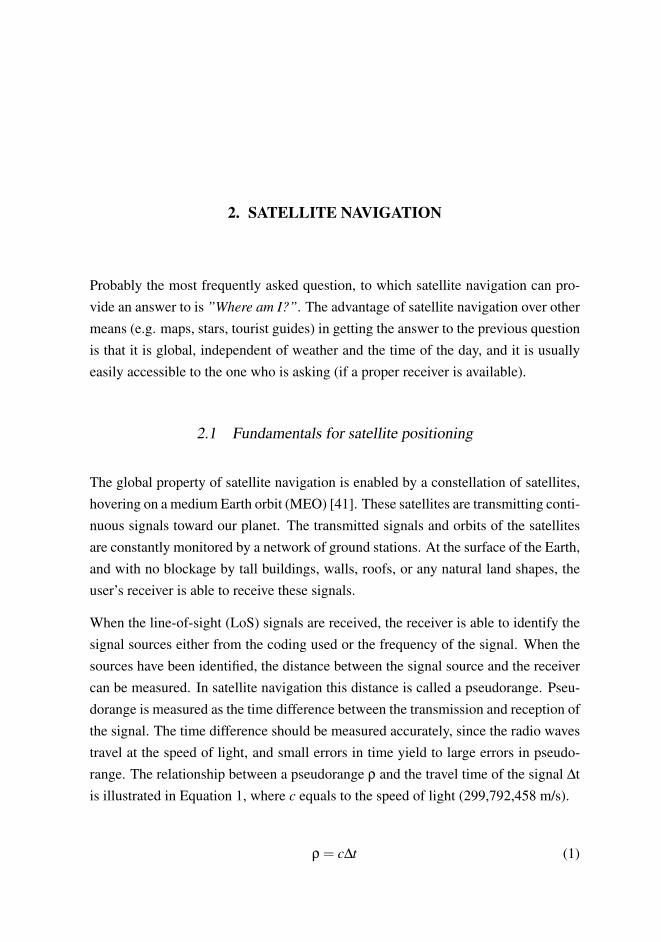
Probably the most frequently asked question, to which satellite navigation can pro-vide an answer to is ”Where am I?”. The advantage of satellite navigation over othermeans (e.g. maps, stars, tourist guides) in getting the answer to the previous questionis that it is global, independent of weather and the time of the day, and it is usuallyeasily accessible to the one who is asking (if a proper receiver is available).
2.1 Fundamentals for satellite positioning
The global property of satellite navigation is enabled by a constellation of satellites,hovering on a medium Earth orbit (MEO) [41]. These satellites are transmitting conti-nuous signals toward our planet. The transmitted signals and orbits of the satellitesare constantly monitored by a network of ground stations. At the surface of the Earth,and with no blockage by tall buildings, walls, roofs, or any natural land shapes, theuser’s receiver is able to receive these signals.
When the line-of-sight (LoS) signals are received, the receiver is able to identify thesignal sources either from the coding used or the frequency of the signal. When thesources have been identified, the distance between the signal source and the receivercan be measured. In satellite navigation this distance is called a pseudorange. Pseu-dorange is measured as the time difference between the transmission and reception ofthe signal. The time difference should be measured accurately, since the radio wavestravel at the speed of light, and small errors in time yield to large errors in pseudo-range. The relationship between a pseudorange ρ and the travel time of the signal ∆tis illustrated in Equation 1, where c equals to the speed of light (299,792,458 m/s).
ρ = c∆t (1)

6 2. Satellite Navigation
After successful determination of four or more pseudoranges, the receiver is ableto estimate its position by using multilateration methods. The relationship betweenmeasured pseudoranges ρi, known satellite locations (xi,yi,zi) and the unknown lo-cation of the receiver (xu,yu,zu) and clock bias bu is illustrated in Equation 2. Clockbias needs to be solved because imperfect clocks in receivers cause too much error inpseudorange measurement.
ρi =√
(xi− xu)2 +(yi− yu)2 +(zi− zu)2 +bu (2)
The previous equations give only the fundamentals for positioning by using satellites.More detailed description of this is well documented in literature, e.g. in [41], [8],and [61]. In practice, the satellite navigation application has been realized already byNAVSTAR Global Positioning System (GPS) in early 1990’s.
2.2 Global Satellite Navigation Systems
In this section global satellite navigation systems are discussed.
2.2.1 GPS
As mentioned before, the American NAVSTAR Global Positioning System (GPS)was the first realization of Global Navigational Satellite System (GNSS). In the li-terature the system is commonly referred to as GPS, without NAVSTAR, and thispractice will be adopted for the rest of this thesis.
GPS’s predecessor was the first space-based navigation system, U.S. navy navigationsatellite system called Transit [41]. Starting from the year 1964, Transit provided atwo-dimensional positioning service, with update rate depending on the user’s lati-tude. The slow update rates of the position fix were suitable for naval navigation, butunsuitable for users with higher dynamics, as aviation and road users.
The previous limitations led to the development of systems for higher dynamics. U.S.Air forces conceptualized System 621B, which introduced some fundamental ideaswhich are still used in satellite navigation, like the usage of pseudorandom noise(PRN) codes for ranging [61].

2.2. Global Satellite Navigation Systems 7
Different from System B621 and Transit, GPS was intented to have dual use, militaryand civilian, from the beginning. Starting from the program establishment in 1969,the GPS developed to gain initial operational capability (IOC) in 1993 and full opera-tional capability (FOC) in 1995 [62]. The FOC status of GPS has continued to thesedays. Standard Positioning Service (SPS) is the service offered to the civilian usersand Precision Positioning Service (PPS) is reserved to military only [41].
The accuracy of the civilian GPS increased with the removal of Selective Availability(SA) in May 2000 [92]. The SA was an intentional degradation of the accuracy ofGPS SPS. This yielded to a sudden increase of the number of civilian users, andnowadays the number of civilian users of GPS is many times higher than the numberof military users.
From a technical point off view, SA was comprised of intentional manipulation of na-vigation data and dithering the satellite clock. This caused variations to pseudorangeerrors, up to 70 meters [62]. The effect of SA is illustrated in Figure 1. There, thesignal captured by researchers from Stanford University and Datum-Irvine was ableto show the exact moment when SA was stopped [27].
GPS achieves global coverage with at least 24 operational satellites circulating Earthin 6 orbital planes located approx. at 20,200 km above Earth’s surface. At the time ofthe writing the constellation included 29 operational satellites of total 32 [87]. Thisarrangement guarantees visibility of 4 to 10 GPS satellites anywhere on the planet,thus enabling global navigation [62], [41].
GPS modernization program is updating the system to meet the 21st Century de-mands of accuracy, availability and reliability. New families of satellites are plannedto launch, carrying new technology and new system features, such as navigation fre-quencies and signals [62].
2.2.2 GLONASS
In parallel with the evolution of U.S. based GPS, the Russian system GLObal’nayaNAvigatsionnaya Sputnikovaya Sistema (GLONASS) was developed. After Cold Warin early 90’s, Soviet Union collapsed and Russia inherited the satellite systems. Rea-soning from political and economical issues, the past development in GLONASS hasnot been as fast as in GPS [62].

8 2. Satellite Navigation
Fig. 1. The termination of GPS Selective Availability c©Datum, Inc., 2000. [27]

2.2. Global Satellite Navigation Systems 9
However, at the time of the writing the development around GLONASS has beenactivated again. Currently, a constellation of 19 GLONASS satellites is available(17 operational, 2 in maintenance [69]), with plans of achieving 24 satellite FOC in2010 [32]. The new modernization rumours include an addition of new signal usingCode Division Multiple Access (CDMA) technique, similar to the one GPS uses. Thelegacy GLONASS is built around Frequency Division Multiple Access (FDMA), sothis would be a big fundamental change. And today, some actors see GLONASS asthe second distinct global satellite navigation system [31].
2.2.3 Galileo
In the early 2000’s the challenge of building European radio navigation system, calledGalileo, was claimed to be as ”The clearest demonstration of the (European) Union’shigher profile in the global transport market” [18]. The same whitepaper [18] alsoidentified the satellite navigation to be a strategically important technology and sta-ted that ”Europe cannot afford to be totally dependent on third countries in a suchstrategic area”.
The development of an European system from those days has been slow, full with de-layed milestones. At the time of writing, the system is in In-Orbit Validation (IOV)phase with two test satellites, called GIOVE-A and GIOVE-B, already in space. Thefirst satellite, GIOVE-A (GIOVE = Galileo In Orbit Validation Element) was laun-ched on the 28th of December at 2005 [20]. The initial objective for this launch wasto secure the frequencies allocated by the International Telecommunications Union(ITU) for the Galileo system [22].
The successor satellite, named GIOVE-B, was launched on the 26th of April in 2008[21]. This satellite carried new clock technology with the first implementations ofnew signal modulations to be used in final system [74].
The final Galileo constellation will consist of 30 satellites, located in three orbitalplanes. The orbits have 56◦ inclination and they are at 23,616 km above Earth’ssurface [62].
The Galileo system will offer several types of services to the users. Open Service(OS) is free of charge, Safety of Life (SoL) is dedicated to emergency services, PublicRegulated Service (PRS) is reserved for non-civilian usage and Commercial Service
10 2. Satellite Navigation
(CS) is offering better position accuracy for those who pay [41].
The European Commission (EC) has identified the areas that are fundamental forGalileo system recognition and market penetration. To support the activities in theseareas, the calls in the 6th Framework Programme (FP6) included topics of Galileouser segment, local elements, introductions of services, thematic support, and appli-cation market development [70]. The activities around Galileo are further supportedin 7th Framework Programme (FP7). This thesis includes work carried out in bothFP6 (GREAT project [71]) and FP7 (GRAMMAR [34], CRISP [81]).
2.2.4 Other sources for satellite navigation
Besides the three systems already discussed, China has shown some interest of buil-ding own systems, called Compass. There exists also plans for regional systems, likeJapanese Quasi-Zenith Satellite System (QZSS) [41].
Satellite based augmentation systems (SBASs) are not standalone navigation sys-tems, but they aim to provide better accuracy for GPS. Augmentations for GPS areWide Area Augmentation System (WAAS) in North America, and European Geosta-tionary Navigation Overlay Service (EGNOS) [62], [41].
2.3 Users of GNSS application
This section discusses the users and industry around GNSS systems.
2.3.1 Use cases for GNSS
As mentioned before, the presidential declaration of removal of Selective Availabilityof GPS in May 2000 affected exponetially to the number of civilian users of GPS.Nowadays, GPS is used in numerous ways, both for work and fun.
Personal navigation
Perhaps the most known form of personal navigation are car navigators. The smallpositioning device telling where to go has become an essential accessory for those
2.3. Users of GNSS application 11
who drive for work (e.g. taxi drivers, truckers) and it also eases the stress when oneis going to holiday by car. Some of the new cars sold today carry an integrated, orin-dash GPS navigator.
Satellite navigation enabled mobile phones, like e.g. Nokia N97, E90 Communicator,6710 Navigator [60], Sony Ericsson W760i [76], and Apple iPhone [2] have beenemerging during last years. These devices have overdriven the standalone personalnavigation devices (PNDs) used mostly by smaller subgroups of users (e.g. hunters,hikers).
The availability of satellite navigation has also created new applications. One off-spring of the technology is the leisure activity called geocaching, where GPS is usedtogether with an internet database to world-wide treasure hunting [35].
Object or person tracking
When satellite navigation is combined with communication technology it can be usedalso to track objects and persons. Asset tracking is one example of this, trains, trucks,and valuable containers can be tracked for better management and increased security[62].
Personal tracking applications are developed for sports, both to enhance training,e.g. [79], and spectator experience in sports like car racing, orienteering, triathlon andcycling. Health and medical applications of satellite navigation include e.g. trackingof persons suffering from Alzheimer’s disease [62]. GPS has also been used foroffender supervision [93].
2.3.2 GNSS industry and markets
With the development of GPS, also the whole new branch of industry - GPS industrywas born. Now the industry is evolving toward GNSS. The drivers for this, originallyU.S. based, industry have been the demands from military, civilian and scientificusers. The GNSS industry players can be divided roughly to two categories; receivermanufacturers and chipset vendors.

12 2. Satellite Navigation
Receiver manufacturers
Receiver manufacturers are companies that make navigation products from thirdparty components. The PND brands like Magellan [54], TomTom [82] and Gar-min [29] are familiar to anyone who has thought about bying a GPS receiver.
Chipset vendors
GNSS chipset vendors are companies that make the integrated circuits (ICs) contai-ning the GNSS receiver functionality. They sell their products to the receiver manu-facturer companies and are not usually recognized by name by an average satellitenavigation user. The smaller companies that offspringed with the navigation tech-nology are in a hard place today. The similar performance of GPS products and thesynergies with other technologies, such as wireless communication [38], are drivingthe big, multitechnology companies to dominate the industry [63].
Market trends
GPS enabled mobile phones is the area of receivers which is the fastest growingin business. It is estimated that in year 2012, 370 million GPS-enabled mobileGSM/WCDMA handsets will be shipped to markets worldwide. This is about 26percent of the total number of phones that will be sold on that year [6]. For compa-rison, the estimate for European sales of PNDs (standalone GNSS receivers) in 2012is 31 million units [5].

3. GNSS SIGNALS AND RECEIVER FUNDAMENTALS
In the previous chapter the application of satellite navigation was described, with theintroduction to application providers and the uses of it. In this chapter a more de-tailed description of how the navigation receivers actually work is given along thedescription of navigation signal characteristics. The GNSS receiver should receivethe signals, find the satellites, measure the pseudoranges and other necessary obser-vations, and then estimate the position, velocity and time (PVT) solution.
3.1 Reception of navigation signals
The essential part of the receiver functionality is to be able to receive signals fromthe desired frequency bands. The challenge in reception is that the satellite signalstravel more than 20 thousand kilometers through space, and when arriving at surfaceof the Earth, they are totally buried under noise.
In this thesis the focus is on GPS and Galileo signals in shared frequency bands,reasoning from the existing availablity of GPS L1 signal (GPS SPS), shared propertyof CDMA based signal structure in both, co-operation between U.S. and Europeannavigation authorities ( [85], [86]), and the project history ( [71], [34]) of the Author.
3.1.1 Navigation frequencies
All satellite navigation signals are located at so called L-band. The IEEE L-band islocated between 1–2 GHz frequencies.
GPS and Galileo frequency bands are illustrated in Figure 2 [19]. From the figure itis clear that the two bands, GPS L1/Galileo E1 centered at 1575.42 MHz and L5/E5acentered at 1176.42 MHz, are of interest when dual frequency receivers are consi-dered. This claim is supported by the results shown in [P7]. There, the analysis

14 3. GNSS signals and receiver fundamentals
Fig. 2. GPS and Galileo signal frequency bands c©ESA/GSA, 2008 [19].
presented shows that the Galileo dual frequency combination of E1/E5a is the mostpromising in terms of acquisition time, power containment in realistic receiver band-witdhs, coherent integration, and best compability with GPS signals.
The implementation cost of dual frequency receiver is discussed in Section 5.2.3 andin [P7].
3.1.2 Antenna
The first part interfacing the signals in a receiver setup is antenna. All GPS and Ga-lileo antennas are characterized by two common factors; they are optimized for righthand circular polarized (RHCP) radiowaves and their radiation (same as reception)pattern is hemispherical. GNSS antennas are usually tuned to receive only a few MHzbandwidth (BW) around the center frequency of the band, and they also may (activeantennas) perform initial amplification of the received signal [41].
3.1.3 Radio-frequency stage
The function of a radio in a GNSS receiver is to perform signal conditioning in sucha way that it can be processed later on in the receiver. A simplified block diagramfor a typical radio is given in Figure 3. First, the incoming signal is filtered and am-plified with a low noise amplifier (LNA), then it is down-converted to a frequency

3.1. Reception of navigation signals 15
Fig. 3. A Simplified block diagram of a radio.
range more suitable for the rest of the receiver. Down-conversion is done by mixingthe incoming signal with a wave from a local oscillator (LO). Then the resultinghigh frequency component ( fsignal + fLO) is filtered out and the remaining low fre-quency component ( fsignal− fLO) is converted to a digital form by an analog-to-digitalconverter (ADC) [41].
Usually the resulting low frequency component is greater than zero, also called inter-mediate frequency (IF). Most of the current GNSS radios are of this type, also knownas heterodyne radio.
The radio illustrated in Figure 3 uses only one LO wave for down-conversion andhas only one ADC output, therefore its outputs are real digital values. Some GNSSradios use also 90◦ phase-shifted version of LO wave to produce additional imagi-nery output from the down-conversion process. In these radios, components afterdown-conversion are duplicated to produce complex digital output (i.e. both real andimaginery values).
Direct conversion
In direct conversion, also known as homodyne radio, the local oscillator producessuch a frequency fLO that it result to a zero center frequency for the desired signaland no IF component remains. The advantages of this architecture over heterodyneradios are that it does not need image rejection, and also the integration using fewercomponents becomes easier. But, these advantages do not come for free. Directconversion brings issues that are non-existing or not so severe in low IF reception.The problems of direct conversion such as DC-offset, LO leakage, I/Q mismatch, arekeeping the IF architecture still more popular [52].

16 3. GNSS signals and receiver fundamentals
Commercial GNSS radio front ends
A few of the currently1 available commercial GNSS RF front end ICs are listed inTable 1 with some selected characteristics. The table contains radios that are eitheractually used in the presented work or referenced in this thesis, for more extensiveoverview of radios, see e.g. [51].
Table 1. Some commercial GNSS RF front ends [3], [58], [72], and [95].Manufacturer RF Band BW [MHz] fIF [MHz] Output
Atmel ATR0603 L1 2 4.123962 Real, 1 bitNemerix NJ1006A L1 3.5 4.188 Real, 2 bits
SiGe SE4210L L1 2.2 or 4.4 near zero Complex, 2+2 bitsZarlink GP2015 L1 1.9 4.309 Real, 2 bits
What comes clear from the previous table is that the output from radio is digital (i.e.the radio contains an ADC), and in low-cost radios typically only one or two bitswide. Multiple bit outputs from radios use sign and magnitude notation.
3.2 Finding the satellites
The navigation satellites can be identified based on their signals. This is possible duethe communication technique called spread spectrum (SS).
The idea behind spread spectrum is to distribute (or spread) the signal over a largefrequency band and transmit it with low power per unit bandwidth. One of the manypossible methods to do this is Direct Sequence (DS) technique. In DS-SS the higherrate chip sequence is modulated to data symbols resulting in a spread band [44].
In Direct Sequence technique pseudorandom noise (PRN) codes are often used, andthis is also the case in code division multiple access (CDMA) systems. In CDMA,each transmitted signal (satellite signal in GNSS case) has its own, unique higherchip rate modulation, or PRN code. From aforementioned systems, GPS and Galileoare CDMA systems, whereas GLONASS is using frequency division multiple ac-cess (FDMA) modulation. In FDMA all signals use the same PRN code, but carrierfrequency is different for each satellite [90], [19], [68].
1 NemeriX filed for bankruptcy in early 2009, and thus their products are no longer available.

3.2. Finding the satellites 17
3.2.1 Ranging codes
In navigation satellite systems, PRN codes are used for ranging. Besides this, theyalso help identify the transmitters and to recover the datasymbols from noisy recep-tion. PRN codes appear to be random signals (i.e. noise), but as the name suggeststhey are only pseudorandom, meaning that they can be generated and reproduced ina controlled way.
GPS L1
In GPS L1 signal, the PRN codes are based on Gold codes [41]. GPS L1 codes arealso often called C/A (Coarse Acquisition) codes, since they were originally devel-oped for helping in the search of the long military codes used in GPS PPS [41]. Goldcodes are generated by a linear feedback shift register (LFSR). The content of LFSRshifts by one bit at each driving pulse (i.e. code clock) and the new input is taken asan exclusive-or (XOR) function of dedicated bits in LFSR. The maximum length ofa generatable bit sequence is 2n−1 bits, where n stands for the length of LFSR. Thegenerated bit sequences appear to have very noise-like statistical properties [33].
The truth table for a XOR function with two inputs is given in Table 2. The functionwith more inputs can be derived from this by cascading two-input XORs, but inprinciple an even number of ones in inputs causes a logical zero at output, whereasan odd number of ones results in a logical one at output.
Table 2. Truth table for logical XOR function.Input A Input B Output
0 0 00 1 11 0 11 1 0
The GPS C/A code generator is illustrated in Figure 4. It consists of two 10-bit longLFSRs (G1 and G2 registers), with feedback polynomials given in Equation 3 and 4.
f1(x) = 1+X3 +X10 (3)

18 3. GNSS signals and receiver fundamentals
f2(x) = 1+X2 +X3 +X6 +X8 +X9 +X10 (4)
There, fi(x) represents the new input value for register Gi and Xn means that the nth
bit value of the register is fed back to the XOR. The equation should be read in a waythat when the content of G1 and G2 registers is set to all ones in reset, the first inputvalue is always zero. This is similar with parity check.
After reset the values of registers start to change, and when the 1023rd(= 210− 1)stage is achieved, the decode logic will generate a new reset. The 1024th stage wouldbe all zeros, fatal to registers to recover.
In GPS C/A case the LFSRs are driven at the speed of 1.023 MHz, which togetherwith the chip count of 1023 results in epoch time of 1 ms. Since GPS data is syn-chronized with PRN generation, the clock for data (50 Hz) is derived from epochfrequency (1 kHz).
In the output of the code generator the last bit of both registers are XOR’red together.The different PRN codes are created by delaying the G2 output by XOR’ing it with adelayed copy of itself. The tapping (or delays) for phase selection logic are given inthe signal specification [90].
GPS L5
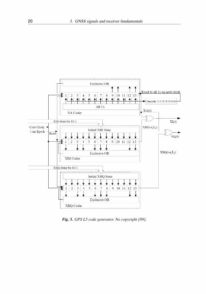
For GPS L5 signals, similar LFSR structure is used for code generation. Unlike GPSL1 signal, the L5 signal contains two PRN codes, one for in-phase (data) and otherfor quadrature-phase (pilot) component of the signal [89]. The code generator for L5is illustrated in Figure 5. In this case, three 13-bit long registers are used to createXIi(t) and XQi(t) outputs. These outputs are 10230 chip long sequences, generatedby XOR’ring 8190 long XA register output with 8191 long outputs from XBI andXBQ.
In this case, the different PRN codes are created by changing the initialization valuesof the XB registers, these initialization values are listed thoroughly in signal speci-fication [89]. The code generation is driven at 10.230 MHz speed, resulting in 1 msepoch periods for L5 codes. The data rate of L5 signals is also 50 Hz, and the signalsalso contain 10/20 symbol Neuman-Hoffman coding [83].

3.2. Finding the satellites 19
Fig. 4. GPS C/A code generator. No copyright [90].
20 3. GNSS signals and receiver fundamentals
Fig. 5. GPS L5 code generator. No copyright [89].

3.2. Finding the satellites 21
Fig. 6. Galileo E5 code generator c©ESA/GSA, 2008 [19].
Galileo E5
Galileo E5 signals (E5a and E5b) are also using code generators for creating PRNcodes. The code generator for Galileo E5 signals is illustrated in Figure 6. ForGalileo E5a/b signals the registers are 14 bits long. All register preset values for E5aand E5b code generation can be found in [19]. Clearly it can be seen that there aresimilarities between code generation in both systems.
Galileo E1
In Galileo E1 OS signals, memory codes are used instead of generatable ones. Me-mory (or random) codes were selected to be used in Galileo E1 OS signals becausethey seemed to offer better cross-correlation properties.
From the implementation point of view memory codes are not that desirable, sincethey need to be saved to the memory of the receiver. In specification [19], 50 code

22 3. GNSS signals and receiver fundamentals
strings for data signal (E1-B) and another 50 for pilot signal (E1-C) are specified.With the codelength of 4092 chips per epoch, the implementation of E1 codes in areceiver will consume approximately 50 kBytes of memory.
Other signals
Out of the GPS signal’s not further discussed in this thesis, modernized GPS L1 Civil(L1C) is by the specification using also LFSRs of length 11 bits, resulting in 1800long codes to be used [91] (i.e. not using the full space). For GPS L2 civil (L2C)signal a different scheme of time-multiplexing long codes (CL) with moderate lengthcodes (CM) is used [26].
3.2.2 Modulation techniques
The pseudorandom code is modulated to the navigation data and further with a carrierwave. In GPS L1 signals, Binary Phase-Shift Keying (BPSK) is used, but for newsignals more navigation specific modulations have been introduced.
Binary Phase-Shift Keying
BPSK modulation is used in GPS L1 [90] and L5 [89], and it will also be used inGalileo E5a and E5b signals [19]. In BPSK the combined data and PRN code waveis multiplied with the carrier, and whenever there is a sign change (assume±1 values)in the coded datastream it results in a 180◦ phase shift in the carrier wave.
Binary Offset Carrier modulations
The origins of BPSK modulation are in communications. Since navigational signalsneed not just to carry data but to maintain precise timing as well, a new modulationtechnique, Binary Offset Carrier (BOC) modulation was presented [7]. In BOC mo-dulation the coded data signal is multiplied with an additional binary subcarrier. TheBOC modulation can be denoted as given in Equation 5, where fs is the subcarrierfrequency, and fc is the code rate. For simplification, fs and fc are often normalizedby the nominal frequency of 1.023 MHz [7].

3.2. Finding the satellites 23
BOC( fs, fc) (5)
Originally, it was BOC(1,1) modulation which was specified for Galileo E1 signals[28]. The agreement with GPS and Galileo authorities further specified the usageof Multiplexed BOC modulation (MBOC) [86]. The MBOC is specified only by itspower spectral density (PSD), which leaves the implementation details open. ForGalileo E1 signals, MBOC is implemented as composite BOC (CBOC), where twoweighted BOC components are added together [19]. The studies over spreading mo-dulations have resulted in a recommendation of using BOC(1,1) with BOC(6,1), acombination which is suitable even for a receiver implementing BOC(1,1) with amaximum penalty of -0.9dB in reception power [37]. The relation of the modulationcomponents of Galileo E1 CBOC modulation is expressed in Equation 6.
1011
(BOC(1,1))+1
11(BOC(6,1)) (6)
3.2.3 Autocorrelation function
The autocorrelation function (ACF) result of PRN modulated signal reaches its maxi-mum when the signal is correlated with a copy of itself having exactly the same phase.When the signal is correlated with a copy having a different phase, the ACF result ismuch lower. ACF for a random binary sequence g(t) is defined in Equation 7 [41].There, R(τ) will reach its maximum when the phase difference (τ) between sequencesis zero.
R(τ) =∫ ∞
−∞g(t)g(t− τ)dt (7)
The autocorrelation functions of future Galileo E1 and E5 signals are given in Figure7. There the dashed red line illustrates the ACF for BPSK modulated signals, GalileoE5a and E5b, and it is similar to the ACF for GPS C/A. For Galileo E1 signal, thecomposite BOC modulation is used and the ACF of it is illustrated with a blue line. Itis clearly visible how BOC modulation creates additional sidepeaks to the ACF. TheGalileo E5 signal uses AltBOC(15,10) modulation, which is illustrated with a blackline.

24 3. GNSS signals and receiver fundamentals
−1 −0.5 0 0.5 10
0.1
0.2
0.3
0.4
0.5
0.6
0.7
0.8
0.9
1
Delay error [chips]
norm
aliz
ed A
CF
env
elop
eACF shapes
E1E5a/E5bE5
Fig. 7. Autocorrelation functions for future Galileo E1 and E5 signals c©IEEE, 2009 [P7].
One must notice that the Figure 7 does not contain time, but only shows the ACFs inrelation to the chip delay error. Due to the different chip rates (see Table 3) the L5and E5 signals have actually a narrower ACF peak in time than the E1 or L1.
3.2.4 Acquisition
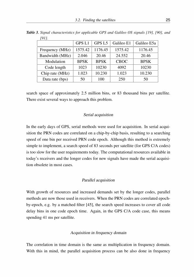
The signal characteristics for GPS and Galileo signals in common frequencies aresummarized in Table 3.
Acquisition is a three-dimensional process to find signal’s identity (or PRN number),code delay and Doppler shift. For example, in GPS L1 receiver this search needsto cover 30 satellites, 2046 code delay bins (in 1
2 chip accuracy) and typically 41Doppler frequency bins (500 Hz per bin, ±10 kHz range) [41]. This results in a
3.2. Finding the satellites 25
Table 3. Signal characteristics for applicable GPS and Galileo OS signals [19], [90], and[91].
GPS L1 GPS L5 Galileo E1 Galileo E5a
Frequency (MHz) 1575.42 1176.45 1575.42 1176.45Bandwidth (MHz) 2.046 20.46 24.552 20.46
Modulation BPSK BPSK CBOC BPSKCode length 1023 10230 4092 10230
Chip rate (MHz) 1.023 10.230 1.023 10.230Data rate (bps) 50 100 250 50
search space of approximately 2.5 million bins, or 83 thousand bins per satellite.There exist several ways to approach this problem.
Serial acquisition
In the early days of GPS, serial methods were used for acquisition. In serial acqui-sition the PRN codes are correlated on a chip-by-chip basis, resulting to a searchingspeed of one bin per received PRN code epoch. Although this method is extremelysimple to implement, a search speed of 83 seconds per satellite (for GPS C/A codes)is too slow for the user requirements today. The computational resources available intoday’s receivers and the longer codes for new signals have made the serial acquisi-tion obsolete in most cases.
Parallel acquisition
With growth of resources and increased demands set by the longer codes, parallelmethods are now those used in receivers. When the PRN codes are correlated epoch-by-epoch, e.g. by a matched filter [45], the search speed increases to cover all codedelay bins in one code epoch time. Again, in the GPS C/A code case, this meansspending 41 ms per satellite.
Acquisition in frequency domain
The correlation in time domain is the same as multiplication in frequency domain.With this in mind, the parallel acquisition process can be also done in frequency

26 3. GNSS signals and receiver fundamentals
Fig. 8. A Block diagram of FFT acquisition.
domain by using Fast Fourier Transform (FFT) for the domain conversion. The blockdiagram of FFT acquisition is given in Figure 8. In the FFT acquisition a block of thesample stream is fed through FFT and multiplied with a complex conjugate of a FFTresult of a local copy of the PRN code. When the resulting complex vector is againtransformed to time domain by inverse FFT, and then squared, result will be the ACF.If the ACF peak is higher than a predefined threshold value, received signal can beforwarded to tracking [8].
Tracking of GNSS signals will be discussed in Section 3.3.2.
3.3 Measuring pseudoranges
”Although providing position, velocity, and time is the ultimate goal of GPS, whenconsidered as a sensor, the receiver’s primary tasks are measurement of range andrange-rate and demodulation of the navigation data” [9].
3.3.1 Measurement breakdown
To enable navigation, the receiver needs to measure pseudoranges to visible satellites.A pseudorange is defined by the time that the signal spends in traveling between asatellite and Earth (See Equation 1). The pseudorange measurement is presented inEquation 8.

3.3. Measuring pseudoranges 27
ρu(t) = c[tu(t)− t(s)(t− τ)] (8)
Where ρu(t) is the pseudorange measurement result, c is the speed of light, tu(t) issignal’s reception time from receiver’s clock and t(s)(t− τ) is signal’s transmissiontime. The signal’s transmission time can be constructed in the receiver from thefollowing measurement information (applies to GPS L1);
• Z-count (equal to GPS time) is a datafield that contains exact time of the weekin seconds, this is transmitted in the navigation data every 6 seconds.
• Number of navigation bits after last received Z-count. With 50 Hz datarate thisgives 20 ms accuracy.
• Number of full C/A code epochs after last received navigation bit. This gives1 ms accuracy.
• Number of full C/A code chips after last full epoch. With 1.023MHz chip ratethis yields to 0.9775 µs accuracy.
• Fraction of remaining C/A code chip. This can be read from the content ofthe numerically controlled oscillator (NCO) driving the code generation anddepends on the sampling frequency of the incoming signal, since usually theNCOs are driven on a sample basis.
The first two items are available only after successful navigation data reception andare taken care by the navigation software. The last three components can be mea-sured from a tracking channel. An analogy between GPS time construction and ananalogue clock is given in [80]. There, Z-count is taken as the hour hand of the clock,navigation bits and code epochs as the minute hand and the remaining is the secondhand.
Even though the previous only discusses GPS L1 signal, the same elements are avai-lable to all other CDMA based signals and thus the pseudorange measurement iscarried out in a similar manner.
28 3. GNSS signals and receiver fundamentals
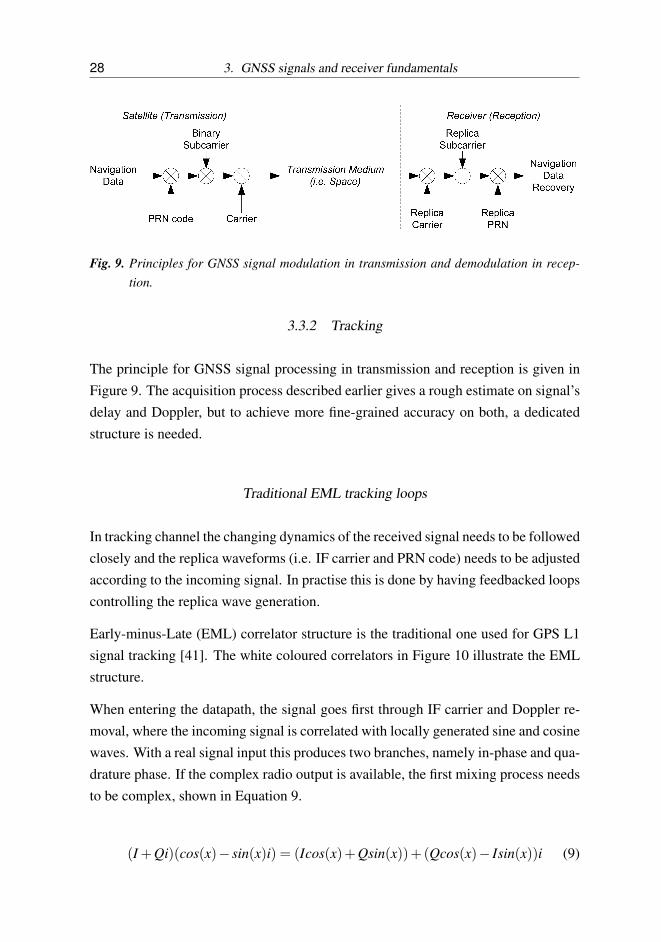
Fig. 9. Principles for GNSS signal modulation in transmission and demodulation in recep-tion.
3.3.2 Tracking
The principle for GNSS signal processing in transmission and reception is given inFigure 9. The acquisition process described earlier gives a rough estimate on signal’sdelay and Doppler, but to achieve more fine-grained accuracy on both, a dedicatedstructure is needed.
Traditional EML tracking loops
In tracking channel the changing dynamics of the received signal needs to be followedclosely and the replica waveforms (i.e. IF carrier and PRN code) needs to be adjustedaccording to the incoming signal. In practise this is done by having feedbacked loopscontrolling the replica wave generation.
Early-minus-Late (EML) correlator structure is the traditional one used for GPS L1signal tracking [41]. The white coloured correlators in Figure 10 illustrate the EMLstructure.
When entering the datapath, the signal goes first through IF carrier and Doppler re-moval, where the incoming signal is correlated with locally generated sine and cosinewaves. With a real signal input this produces two branches, namely in-phase and qua-drature phase. If the complex radio output is available, the first mixing process needsto be complex, shown in Equation 9.
(I +Qi)(cos(x)− sin(x)i) = (Icos(x)+Qsin(x))+(Qcos(x)− Isin(x))i (9)

3.3. Measuring pseudoranges 29
Fig. 10. A diagram of a GNSS tracking channel. White correlators implement EML, darkershaded are additonal ones used for more advanced implementations.

30 3. GNSS signals and receiver fundamentals
Next, the I and Q branches are correlated with locally generated replica code. Codegenerators, exluding Galileo E1 case, can be used to create the local PRN code.The generation is followed by a delay register, that creates closely-spaced delayedversions of the generated code.
The three correlators (namely early, prompt and late) are used by a discriminatorfunction to steer the delay of local PRN replica towards the phase of the incomingsignal. Non-coherent EML power discriminator is given in Equation 10 [41], therethe combined amplitude of the late correlation results (L) is subtracted from the com-bined amplitude of results from the early correlator (E). The I and Q denote in-phaseand quadrature phase branches of the correlator.
12((I2
E +Q2E)− (I2
L +Q2L)) (10)
If prompt correlator (P) is also used as discriminator input, a coherent code discrimi-nator can be applied. The benefit from a coherent loop is its better performance, buton the other hand the code loop becomes dependent on the carrier loop. If the carrierloop is not in lock the coherent code discriminator may fail. Equation 11 [41] showsa coherent dot product discriminator.
12(IE − IE)IP (11)
The discriminators presented in Equations 10 and 11 are used in code loops, or delaylocked loops (DLLs). Besides code, the frequency or phase of the carrier needs also tobe tracked. The locked loops for frequency (FLL) and phase (PLL) take the promptcorrelation results from both I and Q braches as input for the discriminators, likeATAN2 for PLL. For FLL, IP and QP need to be sampled at two time instances tosolve the frequency output error. Typically FLL is used when acquisition hands thesignal over to tracking since it converges faster than PLL, but after that PLL givesmore accurate results [41].
The loops are closed by feeding the filtered discriminator output values to new inputsfor the numerically controlled oscillators (NCOs). NCOs are used to generate thefrequencies needed. NCOs are controlled by the input value, which is accumulateduntil overflow (or underflow if subtracting) occurs. In code NCO this overflow pulse

3.3. Measuring pseudoranges 31
is used as a code generating clock. In carrier NCO, the content of accumulator regis-ters is mapped to sine and cosine waves in such a way that there is one full cycle inthe count range of NCO.
VE-VL
The new modulation techniques introduced to modern GNSS signals bring some is-sues that make them unsuitable for EML correlator. Because of the ACF ambiguitieson BOC family signals, the tracking of future Galileo and GPS (L1C) signals willneed additional correlators (see shaded correlators in Figure 10). These new correla-tors very-early (VE) and very-late (VL) can be used to monitor whether tracking islocked to the main peak or a side peak of the ACF (bump-jumping algorithm) [25],[P1].
In practice the hardware implementation of a code correlator is just a simple XORgate, which is enabled by the sign and magnitude nature of the radio ADC output.The largest addition to complexity when adding more correlators to hardware designis caused by the additional accumulators needed.
Multipath mitigation tracking architectures
The problem of multipath propagation is common to all wireless communications,but its effect to navigation is even worse since it makes accurate timing impossible.Multipaths are reflected copies of LoS signal, and they cause unwanted errors inpseudorange measurements by changing the shape of ACF. This is illustrated in Fi-gure 11, where both constructive multipath (i.e. Non-Los signal is in the same phasethan LoS) and destructive multipath (signals in opposite phases) are illustrated. Da-shed black line represents the ACF of the LoS signal, red dotted line is the ACF of theNLoS signal with 0.7 chip delay and amplitude of half of the LoS case, and solid blueline represents the combined ACF. From the Figure 11 it is obvious that multipathschange the shape of ACF and thus make the determination of the location of the ACFmaximum point more difficult. Multipath is one of the most dominating error sourcesin GNSS positioning [43].
In the EML given in literature [41], the GPS L1 signal the early and late correlatorsare spaced at one chip distance from each other. In practice receivers use narrower

32 3. GNSS signals and receiver fundamentals
−1 0 1−1
−0.5
0
0.5
1
1.5Constructive multipath
Nor
mal
ized
AC
F e
nvel
ope
Delay error [chips]
ACFCombined
ACFLoS
ACFNLoS
−1 0 1−1
−0.5
0
0.5
1
1.5Destructive multipath
Nor
mal
ized
AC
F e
nvel
ope
Delay error [chips]
Fig. 11. Constructive (on left hand side) and destructive (on right hand side) multipath effectswith one NLoS component having delay of 0.7 chips and half of the amplitude of LoS.

3.3. Measuring pseudoranges 33
Fig. 12. A Simplified diagram of Multiple Gate Delay correlator structure, each correlatorpair has its own weighting coefficient an c©IEEE, 2007 [40].
spacing for both multipath mitigation and noise robustness. Tracking implementationwith 0.1 chip early–late spacing is called Narrow EML (NEML) [14].
The additional correlators (VE and VL) can be also used to improve the multipathmitigation (MM) cabability of the tracking channel. Multiple Gate Delay (MGD)structure can be seen as a generalization of correlator based MM algorithms [P3]. Asimplified block diagram of MGD is illustrated in Figure 12. In MGD, more correla-tors are used to form E–L correlator pairs with different spacings. The outputs fromE–L pairs are treated with different weighting factors a, and the spacing betweenearly-late pairs may vary. In [P3], the optimal parameters for MGD weighting andcorrelator spacing with different number of correlators are given. For instance, in thefive correlator case the optimal weighting and spacing seem to be similar with thepatented High Resolution Correlator (HRC) [49].
Multipath error envelopes (MEEs) are a typical criterion used for evaluating the per-formance of the code correlator structures in the multipath environment. Typically,two paths are assumed to be present, and MEEs are calculated versus path spacing inthe noiseless environment. The maximum (positive) multipath errors and minimum(negative) multipath errors occurs when relative NLoS are constructive and destruc-tive with respect to the LoS, respectively. The smaller the enclosed area of the MEEis the better is the theoretical multipath mitigation performance [61], [10], [P2], [P3].
MEEs for NEML, HRC and MGD correlator structures are given in Figure 13. There

34 3. GNSS signals and receiver fundamentals
0 0.5 1 1.5−20
−15
−10
−5
0
5
10
15
20MEEs
Multipath delays [chips]
Cod
e tr
acki
ng e
rror
[met
ers]
NEMLHRCMGD, unifMGD, decr.
Fig. 13. Illustration of the averaged MEEs for NEML, HRC, and two MGDs with optimalparameters as given in [P3] (for uniform and decreasing spacings). Minimum chipspacing of correlator structures is 0.25 chips, and input is noiseless BOC(1,1) signal.
optimum parameters for MGD devived in [P3] are applied. BOC(1,1) modulatedsignal is used as an input.
3.4 Estimating the position
When tracking is locked it should be possible to decode navigation data containinginformation about satellite locations, and to provide baseband measurements neededfor pseudorange formulation. In GPS L1 case the navigation part identifies the Z-count and counts bits occuring after that to create a pseudorange. If also the locationsof satellites are known (ephemeris data has been received) the PVT solution can beestimated. The details how to implement navigation algorithms are out of the scope of

3.4. Estimating the position 35
this thesis, and the theory behind it is well presented e.g. in [41], [8], [61], and [53].
Essentially, navigation software tries to solve the best estimates for the four unk-nowns presented in Equation 2. To achieve this, a few iterations are needed. Toimprove the quality of the result, more advanced methods, like Kalman filtering canbe used. Also the reliability of the solution may be increased by using dedicated algo-rithms to exclude erroneous pseudorange measurements out from the solution [42].

36 3. GNSS signals and receiver fundamentals

4. GNSS RECEIVER TOOLS
The tools for GNSS receiver research can be divided to two categories; link leveltools and multi-channel simulators. Both types of the tools are covered in discussiongiven in this chapter.
4.1 Link level tools
Link level tools are modelling a single channel, from transmitter to receiver, and arecapable for producing a single pseudorandom measurement, and thus incapable forproducing full PVT solutions. Link level tools are applicable, e.g., for testing andvalidation of new baseband algorithms.
4.1.1 GRANADA
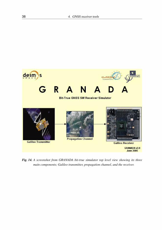
GRANADA (Galileo Receiver ANAlysis and Design Application) is developed byDeimos Space. The tool was one of the outputs from the GARDA (GAlileo ReceiverDevelopment Activities) EC FP6 project [46]. GRANADA is a Matlab/Simulink [47]based software that originally contained two tools, a bit-true simulator and an Envi-ronment and Navigation simulator (E&N). Later, a supplementary Factored Corre-lator Model (FCM) blockset was introduced [73]. Currently, GRANADA is one ofthe very few commercially available link level simulator software tools for Galileorecearch.
From the receiver algorithm development point of view the most interesting is thebit-true simulator, which models the signal chain from satellite to receiver. An illus-tration of GRANADA bit-true simulator blocks is given in Figure 14.
In the early stages the users of the GRANADA software were mainly the researchersfrom the GARDA project. GRANADA was introduced in [24], presenting measure-
38 4. GNSS receiver tools
Fig. 14. A screenshot from GRANADA bit-true simulator top level view showing its threemain components; Galileo transmitter, propagation channel, and the receiver.

4.2. Multi-channel simulators 39
ments on the Galileo receiver’s performance under GPS interference and multipathconditions. The tool was used to validate the novel BOC tracking technique in [13],and to analyze the code Doppler shifts on Galileo E5 and E1 OS signals [15].
After the GARDA project, the usage of GRANADA tool was also adopted by re-searchers involved with the GREAT project. There it was used for validating MGDalgorithms presented in [40], [P3]. The issue on the non-repeatability property ofGRANADA bit-true simulator was raised and solved in [P2].
4.1.2 SMOG
SMOG (Simulink Model Of Galileo) is a tool developed in Tampere University ofTechnology, more precisely in Department of Computer Systems. It was developedduring the GREAT EC FP6 project to complement the research in the period of una-vailability of the GRANADA software. The structure of the SMOG tool is similarwith GRANADA; transmitter - channel - receiver. The tool is described in detailsin [64].
Current development of the SMOG tool is frozen to the C++ accelerated Matlabversion. In this version the intellectual properties (IPs) developed within Simulinkhave been moved to Matlab with certain parts of the application modelled as C++to speed up the simulations. This upgraded tool was used in [P4], to perform thebaseband functions (acquisition and tracking) to recorded real navigation signals.
4.2 Multi-channel simulators
Multi-channel simulators are capable of processing multi-channel data, and thus theycan provide pseudorange measurement results with a PVT solution. Post-processingreceivers are an example of tools belonging to this category. Increased availability ofUSB-based GNSS RF front ends has affected the popularity and evolution of the postprocessing GNSS receiver tools [94].
4.2.1 DGC SDR GPS
A post processing GPS receiver from the Danish GPS Center (DGC) was publishedalong with the Software Defined Radio (SDR) GPS receiver book [8]. The book

40 4. GNSS receiver tools
contains a DVD with receiver Matlab codes and a few example data sets. The recei-ver is accompanied with a radio front end module manufactured by SiGe, which isavailable for purchasing through the book’s webpage [88].
DGC SDR GPS reads the raw data from a file and thus it is independent of the datasource, if the data format is suitable for the receiver. The receiver is implementedfully in Matlab environment with having fully accessible codes, which makes it easyto approach and thus well suited e.g. for education and research. On the other hand,only Matlab based implementation has extremely slow execution.
4.2.2 Namuru Receiver
The Namuru receiver is developed at the University of New South Wales (UNSW),Australia. The receiver is implemented on an FPGA platform, thus allowing the ba-seband processing hardware to be completely customised by the user. The hardwareis implemented with VHDL and Verilog hardware desctiption languages [57].
The original Namuru was GPS L1-only receiver. The second version, Namuru II, hasadded the ability to receive also L2 signals. Both versions are based on an AlteraFPGA platform containing memories (Flash, SRAM, and SDRAM) and peripherals(RS232, USB, RTC, GP I/O, and IMU), and are compatible with Zarlink GP2015 RFfront end [95]. The block diagram of Namuru II architecture [30] is shown in Figure15.
4.2.3 NavX-NSR
NavX-NSR is a GPS/Galileo L1/E1 software receiver created by IFEN GmbH. Thereceiver can operate in both real-time and post-processing modes. The receiver hard-ware incorporates a RF front end with an integrated Field Programmable Gate Array(FPGA) and a USB interface. The accompanying software introduces applicationprogramming interfaces (APIs), which the user can use to control over 200 parame-ters of the receiver [39]. Even though the APIs offer a high degree of flexibility, theyseem not to give full control over the receiver hardware to the user.

4.2. Multi-channel simulators 41
Fig. 15. A block digram of the Namuru V2 architecture c©General Dynamics Corporation,2009 [30].
42 4. GNSS receiver tools
4.2.4 N-Gene
N-Gene is a GPS/Galileo software receiver tool developed in NavSAS (NavigationSignal Analysis and Simulation) group, at the Navigation Laboratory of Politecnicodi Torino, Italy. The receiver is GPS/Galileo L1/E1 signal compatible and it canalso demodulate signals from EGNOS system on same frequency. Even being fullyimplemented in software it is capable of processing GNSS signals in real-time. TheN-Gene has an modular software architecture, allowing it to be modified for e.g. fordifferent radio front ends and other research driven purposes [23].
4.2.5 GNSS Receiver Reference Design - TUTGNSS
GNSS Receiver Reference Design resulted from accumulated receiver research anddevelopment work carried out in Tampere University of Technology, at the Depart-ment of Computer Systems. The starting point for the receiver desing was a collectionof discrete hardware IP blocks, created by many members of the group. The first trialswith a commercial radio, Nemerix NJ1006A [58] were the enablers for performingtests with real signals. The real signal records were forwarded to separate basebandprocessing (C++ accelerated Matlab SMOG) and a separate navigation computationwas executed from measured pseudoranges and data. In parallel, hardware basebanddevelopment was done with an FPGA platform [P4].
Later, all tasks were further integrated to a first real-time receiver implementation,called TUTGNSS. TUTGNSS is implemented on an Altera FPGA board and it usesa NIOS-II softcore processor for closing the tracking loops and computing the navi-gation solution. The hardware is fully reconfigurable, and the receiver is independentof the radio brand (currently SiGE SE4120L [72] and Atmel ATR0603 [3] are used),thanks to its baseband converter unit (BCU) [66]. Currently, TUTGNSS is used as abaseline for advanced Galileo receiver implementation in the GRAMMAR project.
4.2.6 C++ TUTGNSS
C++ TUTGNSS is a real-time software receiver, originally developed to model multi-core execution of GNSS applications. This receiver is implemented in a C++ envi-ronment and it is exploiting parallelism via thread processing. E.g. for baseband,

4.2. Multi-channel simulators 43
three processes are identified and implemented as separate threads; input preproces-sing, which removes the IF and performs signal decimation if necessary, acquisition,which searches for all visible satellites with an FFT method, and tracking, whichtracks satellites and extracts navigation data bits and measures the pseudoranges [65].
C++ TUTGNSS was used to acquire some of the results presented in [P6].

44 4. GNSS receiver tools

5. ARCHITECTURAL CONSIDERATIONS FOR GNSS RECEIVERS
In this chapter, the receiver architectures are discussed, but first some general designrequirements for embedded systems are revised.
5.1 Common design requirements for embedded receivers
This section provides a discussion about common design requirements for embeddedreceivers to support the content given in Section 5.2.
5.1.1 Processing power
Processing power means the workload that the central processing unit (CPU) of thereceiver can handle. It is commonly expressed as a million instructions per second(MIPS) rating [4]. Another issue affecting the processing power is how many bits areprocessed per instruction. Register word length of the processor included in today’sreceivers is typically 32 bits (e.g. ARM7 family [36]).
5.1.2 Memory
The memory in embedded systems holds both program code and data. The amountof available memory may be closely tied to the wordlength of the registers of the pro-cessor, since wordlength establishes an upper limit to the memory size. For example,16-bit registers can address only 64 kBytes of memory (216) [4].
In 32 bit-architecture, the memory address limitation is not a problem (theoreticalupper limit is over 4 GBytes), but still the downsides that come with larger memoryfootprint are present; higher cost, larger power consumption, and greater physical
46 5. Architectural considerations for GNSS receivers
size [78]. These are keeping the practical memory size of an embedded device quitesmall.
5.1.3 Power consumption
Power consumption is important especially in battery operated devices, which hand-held devices usually are. Powerful batteries tend to increase the weight of the device,and thus it is more practical to focus on decreasing power consumption than increa-sing battery capacity. Large power consumption also causes noticeable heating whichis not a desirable effect e.g. for a mobile phone. An approximate 3W maximum li-mit for the power density in a cellular device is given in [59]. The relation betweencomputational power and electrical power consumption in embedded systems is quiteoften expressed as MIPS per milliwatt (MIPS/mW) [67].
5.1.4 Cost
The cost might be the most important factor when considering mass markets. Theactual cost of a full device consists of multiple variables, ranging from developmentto marketing cost. However, on hardware level, unit cost is usually used as a mea-sure. Today the cost of a GPS chip inside a receiver is approximately 1 U.S. dollar. Inapplication specific integrated circuits (ASIC), which GPS chips also are, the biggestcosts come from nonrecurring engineering (NRE), which is basically a large one timedevelopment and manufacturing set-up cost. If generalized, the cost for manufactu-ring one GPS chip is as large as for ten thousand ones. So, it becomes clear that inchipsets it is the production volume that lowers the cost.
5.2 Overview of receiver architectures
In this section an overview of GNSS receiver architectures is given and discussed inligth of design requirements discussed earlier.

5.2. Overview of receiver architectures 47
5.2.1 State-of-the-art GNSS receivers
Current state-of-the-art mass market receivers are based on a chipset or single-chipreceiver [48]. The chipset or single-chip receiver is usually implemented as an ASIC.Hardware implementation of a baseband engine is stemming from the high compu-tational demand of tracking. One-channel tracking takes approximately 10 MIPS toreach real-time [75].
In high volume production ASICs are cheap, and they can also be optimized forsmall size and to have low power consumption. FPGA technology has not emergedin commercial, everyday receivers, but it has found its place in receivers targeted forresearch, e.g. in [17] and [P4].
There are no commercial dual-frequency receivers for L1/L5 combination availableat the moment. Some of the manufacturers declare their products to be Galileo-ready,but most of the available chipsets are for GPS only.
UBX-G5010
Swiss chipset manufacturer U-Blox has presented a GPS and Galileo-ready singlechip receiver. This 50-channel receiver is stated to have over a million correlators.Product datasheet reveals an architecture containing a dedicated GPS/Galileo hard-ware engine, an ARM7 CPU, memories and peripherals. The power consumption isdeclared to be 64 mW in tracking mode [84].
Teseo
The Teseo platform is a high-sensitivity standalone GPS solution belonging to STMi-croelectronics’ product portfolio. This chipset consists of GPS baseband, embedded-Flash device, and an RF front-end. The baseband combines an ARM7 32-bit mi-crocontroller and a high-performance GPS engine (HPGPS) with a wide range ofperipherals [77].
48 5. Architectural considerations for GNSS receivers
SiRFstarIII
SiRFstar III is one of the most used GPS chipsets in commercial receivers. The latestversions GSC3e/LPx and GSC3f/LPx are characterized by having up to 20 channelsand power consumption of 46 mW in autonomous reception. The architecture isbased on a GPS engine and ARM7 CPU [11].
SiRFstarIV
The biggest change from SiRFstarIII to SiRFstarIV is in the architecture. The fourthgeneration of chips is following the host-based architecture, where the navigationcomputation is moved from the chip to the host processor. This solution lowers thebill-of-material (BOM) costs. The 48-channel receiver introduces 5 to 6 MIPS loadsto the host processor [12].
5.2.2 Towards SDR
In Software Defined Radio (SDR) the hardware problems are turned into softwareproblems. In theory this means that everything after ADC should be done by soft-ware, but in practice there are many views on this. The concept of SDR was presentedin the early 1990’s [55], about same time when GPS turned operational. After thatthe usage of SDR in GNSS is discussed widely in literature, e.g. in [1], [17], [94],and [8].
The well-known Moore’s law [56] is stating that the capacity of integrated circuitsis doubling every 18-24 months. This claim has proven to be true for the last 3or 4 decades. In this light, ideal SDR solutions should become feasible eventuallywhen available processing power increases. Currently reported SDR GPS receiverimplementations are working in real-time only if the clock speed of the processor isfrom 900 MHz [75] to 3 GHz [16], which is too high for mobile devices but not, forexample, for a laptop PC.

5.2. Overview of receiver architectures 49
Fig. 16. Hardware cost vs software complexity (in MIPS) in GPS receiver architecturec©Soderholm, 2008 [75].
Hardware cost vs. software complexity
In a GNSS receiver, (or in general any receiver), the shift from hardware towardssoftware implementation does not come for free. When hardware cost is reduced bymoving tasks to software, it increases the complexity of software. The relationshipbetween receiver cost and software complexity is illustrated in Figure 16 [75].
The figure estimates that moving from hardware accelerated to pure software solutionwill increase the complexity of software (MIPS figures) by a factor of ten. This wouldalso mean that the processor should be capable of executing ten times more program,resulting in a need for higher clock frequency and/or more optimized processor ar-chitecture. Increase in MIPS count will also mean an increase in power consumptionand heat generation.
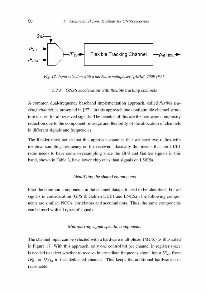
50 5. Architectural considerations for GNSS receivers
Fig. 17. Input selection with a hardware multiplexer c©IEEE, 2009 [P7].
5.2.3 GNSS acceleration with flexible tracking channels
A common dual-frequency baseband implementation approach, called flexible tra-cking channel, is presented in [P7]. In this approach one configurable channel struc-ture is used for all received signals. The benefits of this are the hardware complexityreduction due to the component re-usage and flexibility of the allocation of channelsin different signals and frequencies.
The Reader must notice that this approach assumes that we have two radios withidentical sampling frequency on the receiver. Basically this means that the L1/E1radio needs to have some oversampling since the GPS and Galileo signals in thisband, shown in Table 3, have lower chip rates than signals on L5/E5a.
Identifying the shared components
First the common components in the channel datapath need to be identified. For allsignals in consideration (GPS & Galileo L1/E1 and L5/E5a), the following compo-nents are similar: NCOs, correlators and accumulators. Thus, the same componentscan be used with all types of signals.
Multiplexing signal specific components
The channel input can be selected with a hardware multiplexer (MUX) as illustratedin Figure 17. With this approach, only one control bit per channel in register spaceis needed to select whether to receive intermediate frequency signal input IFSel fromIFE1 or IFE5a to that dedicated channel. This keeps the additional hardware costreasonable.

5.2. Overview of receiver architectures 51
Fig. 18. The structure for a generic flexible tracking channel c©IEEE, 2009 [P7].
The flexible tracking channel concept is illustrated in Figure 18. Here, NCOs are usedto produce the frequencies needed, and they are controlled by the software control.The components producing local code and additional modulation (BPSK does notintroduce additional modulation here, whereas BOC family modulations will) arealso selected with hardware MUXes, again using only a few bits of the total controlregister space of the receiver.
Further size optimization
Combining the synergies of code generation, illustrated in Figures 4, 5 and 6, theintegration level of multi-system and multi-frequency baseband could be increased.Basically, a common LFSR structure with long enough registers, and reconfigurablefeedback could implement all generatable PRN codes known in shared GPS/Galileofrequencies. Of course, the Galileo E1 memory codes are not compatible with this
52 5. Architectural considerations for GNSS receivers
approach.
5.2.4 SDR with multiple cores
An SDR receiver with multiple cores within the context of GNSS is a novel imple-mentation approach. To the Author’s knowledge the studies on this topic presentedin [P5] and [P6] are unique.
In the multiple core approach, the computational load of correlation is divided tomultiple Very Long Instruction Word (VLIW) cores. VLIW is a CPU architecturethat exploits instruction level parallelism (ILP) [50]. This receiver architecture com-bines the advantages of the SDR; the flexibility and upgradeability, with having moreMIPS/mW available. Multiple cores are suitable for multitechnology devices sincethe same array of cores can be used to also process the other streams, like multimediaand wireless communication.
Multicore platform
Multicore SDR is a platform containing a number of dedicated reconfigurable VLIWDigital Signal Processors (DSPs). Each core is communicating via a Network-on-Chip (NoC) with other DSPs, global memories and peripheral interfaces. The GNSSradio front end is interfaced to the parallel interface of the NoC through some inter-face logic.
GNSS application in multicore platform
Three main processes for baseband operation are identified; input preprocessing, ac-quisition and tracking [65]. Input preprocessing takes care of down-conversion andtime-stamping of incoming stream packets. Multiple FFT acquisition processes arestarted dynamically, and tracking processes are initialized when satellites are found.An example mapping of a GNSS application on to a multicore platform at a certaintime instance is given in Figure 19.
The navigation software is executed in General Purpose Processor (GPP), interfacedto a NoC. Finally, a PC is used to illustrate the receiver output.

5.2. Overview of receiver architectures 53
Fig. 19. SDR GNSS application mapped on to a multicore platform.

54 5. Architectural considerations for GNSS receivers
The analysis provided in [P5] and [P6] proves that the current approach is feasibleto be implemented. In [P5], the complexity of the GNSS application’s basebandprocesses in terms of computation were analyzed and compared to the reported per-formance of the VLIW cores. There it was shown that the targeted platform hascapability to process GNSS baseband functions, acquisition and tracking. This ana-lysis was extended in [P6] to contain also the communication payload requirement ofthe NoC.
This thesis does not hold data from the implementation of such a multicore GNSSSDR, but the implementation will follow, as the project [81] where this topic is dealtwith proceeds.

6. SUMMARY OF PUBLICATIONS
This chapter contains a summary of the enclosed publications with a description ofAuthor’s contribution.
6.1 General
All of the enclosed publications are naturally from the area of satellite navigation andpositioning receivers. The publications were made between 2006 and 2009, while theAuthor has been carrying out the research work and post-graduate studies in Tam-pere University of Technology, Department of Computer Systems. From the sevenenclosed publications, five are published as papers in the proceedings of internationalconferences and two as articles in international journals. None of the enclosed publi-cations has been previously used as a part of any academic thesis or dissemination.
6.2 Overview of the publication results
The work presented in the enclosed publications has significance for the GNSS re-searcher community by giving contribution to unification of the GRANADA researchtool. The presented studies of issues of the combined GPS/Galileo receivers are to-pical due to upcoming deployment of Galileo system. And finally, the thesis hassignificance by presenting a novel multiple core approach for SDR GNSS receiversgiving also the analysis of its implementation feasibility.
The results of the publications enclosed to this thesis can be summarized with thefollowing points:
• Simulation tools play a vital role in development of new receiver algorithms(e.g. for multipath mitigation), especially when systems are not yet existing

56 6. Summary of Publications
(like Galileo at the time of writing). From this point of view the researcherswould benefit of having a standard set of tools, which would make the resultsachieved in different entities and studies comparable [P2], [P3].
• In receiver algorithm development the gap between high level simulations andlow level implementations should be also considered; one solution for this isseen to be the usage of FPGA based platforms to address also the hardwarepoint of view [P3], [P4].
• The implementation of multi-system and multi-frequency receiver basebandsbenefits from using flexible structures. High level of re-usability (only theessential components are duplicated) makes this approach favourable in appli-cations where implementation size and cost matter [P1], [P7].
• Multiple core receiver implementation seems to offer a good balance betweenflexibility and upgradeability needed for new satellite navigation systems andalgorithms, and when properly designed and scaled, a reasonably low unit pricein high volume production [P6].
• It is shown that multiple core platform is suiting well for GNSS signal proces-sing from a computational point of view [P5], [P6].
6.3 Author’s contribution to publications
In the beginning of this thesis work there was a short period when the Author was theonly member of the current GNSS group under professor Nurmi’s supervision. Sincethen, people have been coming and going and the group size and status has increasedsignificantly from the early days. Working with other people has been essential fordevelopment of ideas and innovations. Quite many papers have been born in casualconversations over a coffee, where discussion of not work-related issues were carriedout as well.
Besides own group, the collaboration with people from Department of Communica-tions Engineering, especially Docent Elena-Simona Lohan, has been fruitful. Wor-king with international projects, like GREAT, CRISP, and GRAMMAR have alsogiven an important medium to connect with professionals and experts in many fields

6.3. Author’s contribution to publications 57
of technology, which has been forwarded as an invaluable input to the research andits outcomes.
The Author acknowledges that all of the co-authors have contributed to the final ap-pearance of each publication enclosed here. All of the co-authors have seen andagreed with the following descriptions of the Author’s contribution.
The main contributions of the Author to the publications are as follows:
In [P1], the Author implemented the SystemC model used and wrote the manuscript.The idea for the paper came from the Author.
In [P2], the Author was the main contributor to the manuscript and originated the ideaof writing it. The Author also executed simulations to verify the presented modifi-cations to the GRANADA tool. The original problem, to which this paper presentedthe solution, was pointed out by Jussi Raasakka. Other co-authors contributed byimplementing the tools used, and also revising the content and language of the paper.
In [P3], the Author was the main contributor to the manuscript. The Author alsoimplemented the SystemC model used and simulated and analyzed both SystemCand VHDL model simulations and results. The idea for the computational methodsfor finding optimal MGD parameters and also motivation for writing the article camefrom Docent Elena-Simona Lohan.
In [P4], the Author was the main contributor to the manuscript. The idea for ”GNSSReceiver Reference Design” and the paper originated from the Author.
In [P5], the Author was the main contributor to the manuscript. The work presentedin this publication was carried out by the Author. The idea for the paper came fromthe Author.
In [P6], the Author was the main contributor to the manuscript. The work, excludingthe implementation of the real-time SW GPS receiver tool, was carried out by theAuthor. The idea for this publication originated from the Author.
In [P7], the Author was the main contributor to the manuscript. The work for ba-seband implementation issues analysis was carried out by the Author. The idea andmotivation for this publication originated from Docent Elena-Simona Lohan.

58 6. Summary of Publications

7. CONCLUSIONS
This introduction provided in Chapters 1 through 7 together with the enclosed publi-cations presents the Author’s research work and results. The research area belongs tothe area of global satellite navigation, where the focus is on future GNSS receivers,more precisely on multi system and multi frequency issues on mass market receivers,where low cost and power consumption are dominating parameters. The presentedresearch is contributing to this area by enhancing receiver research tools and givingpotential architectural considerations.
7.1 Main Results
The main results and contributions of the research reported in this thesis are:
Simulation tools play an invaluable role in research and development of receivers,especially for systems that have no, or only a reduced set of, real signals availableyet. Analysis of available simulation tools for GNSS receiver R&D was presentedin the thesis. From this point of view the key is to have a standardized environmentfor research, that would make the results achieved in different entities and studies tobe comparable. In this thesis work, a significant issue of the non-repeatability of theGRANADA tool was raised and solved [P2].
In this thesis studies on combined GPS/Galileo receivers were presented. Implemen-tation of a feasible multi-system baseband architecture for mass market receivers ispossible, thanks to the similar structure of CDMA-based signals in both systems [P1].A similar approach can be used to make baseband solutions for multi-frequency pro-cessing. In both cases, a flexible approach by re-using all shared components andhaving only signal specific components as additional implementation [P7]. For low-cost solutions, Galileo E1 memory codes are not favourable due to their memory

60 7. Conclusions
consumption. FPGAs offer a good platform to test the non-functional requirementsof baseband implementations [P3], [P4].
The term Software Defined Radio covers a wide set of different architectures. Fromthe presented ones, a SDR receiver with a hardware correlator engine seems to be thestate-of-the-art solution in handheld devices. The development defined by Moore’slaw is enabling pure real-time software GNSS receivers in laptop computers, and thedirection is to transfer the software solution into smaller devices. This thesis presen-ted a novel approach, SDR implementation with multiple cores, which seems to offera good platform having flexibility and upgradeability needed for new satellite naviga-tion systems and algorithms. The presented work proposes that from a computationalpoint of view multi-core platforms are well-suited for GNSS signal processing [P5],[P6].
7.2 Future Trends
In future, GNSS will probably find its way to almost everywhere. If compared to digi-tal camera, which nowadays is almost a standard feature in any mobile device, GNSSreceiver might end up to having the same status. At least, in the devices containingwireless technology, it is encouraged to have also GNSS on board. With the deve-lopment in radio technology and exploitation of synergies between positioning andcommunication technologies this might yield to almost a zero BOM cost addition.
In a multicore SDR approach, the realization of GNSS application and the platformare happening in the foreseeable future and the results achieved will be documentedand submitted to scientific publications forums.
Besides technology, new unforeseen applications are most likely arising from scratch.Geocathing is a good example of an application that emerged when technology madeit possible. Also, this is probably the direction where investors are looking towardssince the receiver ICs or IPs can be integrated only in a finite (yet a large) number ofdevices, whereas there is no limit seen for applications.
The time of the research presented has been interesting since it has gone side by sidewith the Galileo system development. The realization of all given promises is some-thing to look for, and the alignment between (or order of) the three major satellitenavigation systems, GPS, Galileo, and GLONASS, is something that is not seen yet.

7.2. Future Trends 61
Also the role of the planned Chinese system and emerging local augmentations willbe interesting to follow also from the receiver development point of view.

62 7. Conclusions
BIBLIOGRAPHY
[1] D. Akos, “The role of Global Navigation Satellite System (GNSS) softwareradios in embedded systems,” GPS Solutions, May 2003.
[2] “Apple webpage,” http:www.apple.com, Apple Inc., Aug. 2009.
[3] Atmel, “ATR0603 - GPS Front End IC,” Datasheet. Rev 3.5, Nov. 2006.
[4] M. Barr and A. Massa, Programming Embedded Systems: with C and GNUdevelopment tools. O’Reilly Media, 2006.
[5] Berg Insight, “Connected Navigation Devices,” Nov. 2007, LBS Research Se-ries.
[6] Berg Insight, “GPS and Mobile Handsets,” Jan. 2008, LBS Research Series.
[7] J. W. Betz, “Binary Offset Carrier Modulations for Radionavigation,” Naviga-tion: Journal of Institute of Navigation, vol. 48, no. 4, pp. 227–246, 2001–2002.
[8] K. Borre, D. Akos, N. Bertelsen, P. Rinder, and S. Jensen, A Software DefinedGPS and Galileo Receiver - A Single-Frequency Approach. Birkhauser, 2007.
[9] M. Braasch and A. J. van Dierendonck, “GPS Receiver Architectures and Mea-surements,” Proceedings of the IEEE, vol. 87, no. 1, pp. 48–64, Jan 1999.
[10] A. Burian, “Reduced-Complexity Code Synchronization in Multipath Channelsfor BOC Modulated CDMA Signals with Applications in Galileo and Moderni-zed GPS Systems,” Ph.D. dissertation, Tampere university of Technology, 2009.
[11] CSR, “SiRFstarIII GSC3e/LPx & GSC3f/LPx - Flag-ship Performance, Lowest Power Flash GPS Solution,”http://www.csr.com/products/sirfstar gsc3eLPx.htm, Sep. 2009.

64 Bibliography
[12] CSR, “SiRFstarIV GSD4t - Host-based GPS Receiver Featuring SiRFawareTechnology,” http://www.csr.com/products/sirfstariv.htm, Sep. 2009.
[13] D. de Castro, J. Diez, A. Fernandez, and J. Sleewaegen, “A New UnambiguousLow-Complexity BOC Tracking Technique,” in Proc. 19th International Tech-nical Meeting of the Satellite Division of the Institute of Navigation ION GNSS2006ION GNSS, Sep. 26–29, 2006, pp. 1830–1835.
[14] A. V. Dierendonck, P. Fenton, and T. Ford, “Theory and performance of narrowcorrelator spacing in a GPS receiver,” Journal of the Institute of Navigation,vol. 39, no. 3, pp. 265–283, Fall 1992.
[15] J. Diez, A. Fernandez, D. Fossati, L. Marradi, and Gabaglio, “Using the GRA-NADA Bit-True Simulator to analyse the effect of Code Doppler shift in GalileoE5 and L1 Receivers,” in Proc. ENC GNSS 2005, Munich, Germany, Jul. 19–22,2005.
[16] C. Dionisio, L. Cucchi, and R. Marracci, “SOFTREC G3, Software Receiverand Signal Analysis fog GNSS Bands,” in Proc. 2008 IEEE 10th InternationlSymposium on Spread Spectrum Techniques and Applications (ISSSTA), Bolo-gna, Italy, Aug 2008.
[17] F. Dovis, A. Gramazio, and P. Mulassano, “SDR Technology Applied to GalileoReceivers,” in Proc. 15th International Technical Meeting of the Satellite Divi-sion of the Institute of Navigation ION GPS 2002, Portland, OR, Sep. 24–27,2002, pp. 2566–2575.
[18] European Commission, “European transport policy for 2010: time to decide,”Sep. 2001.
[19] “Galileo Open Service, Signal In Space Interface Control Document (OS SISICD),” European GNSS Supervisory Authority, Feb. 2008, draft 1.
[20] European Space Agency, “GIOVE A,” http://www.giove.esa.int/page index.php?menu=102&page id=35, Jun. 2009.
[21] European Space Agency, “GIOVE B,” http://www.giove.esa.int/page index.php?menu=103&page id=36, Jun. 2009.
Bibliography 65
[22] M. Falcone, M. Lugert, M. Malik, M. Crisci, E. Rooney, C. Jackson, andM. Threteway, “GIOVE-A In Orbit Testing Results,” in Proc. 19th Interna-tional Technical Meeting of the Satellite Division of the Institute of NavigationION GNSS 2006, Fort Worth, TX, Sep. 26–29, 2006.
[23] M. Fantino, A. Molino, and M. Nicola, “N-Gene GNSS Receiver: Benefits ofSoftware Radio in Navigation,” in Proc. ENC-GNSS 2009, Naples, Italy, May3–6, 2009.
[24] A. Fernandez, J. Diez, L. Marradi, and V. Gabaglio, “Galileo Receiver Perfor-mance Under GPS Interference and Multipath With the GRANADA SoftwareReceiver,” in Proc. 17th International Technical Meeting of the Satellite Divi-sion of the Institute of Navigation ION GNSS 2004, Long Beach, California,Sep. ,21–24 2004, pp. 1027–1034.
[25] P. Fine and W. Wilson, “Tracking algorithms for GPS Offset Carrier signals,”in Proc. 1999 National Technical Meeting of the Institute of Navigation, SanDiego, California, Jan.25–27 1999, pp. 671–676.
[26] R. Fontana, W. Cheung, and T. Stansell, “The modernized L2C signal - Leapingforward into the 21st century,” GPS World, pp. 28–34, Sep 2001.
[27] R. Fuller, E. Fudurich, and F. Weiler, “GPS Without Selective Availability,”whitepaper, May 2000, http://www.timingtechnologies.com/Gpswp1.pdf.
[28] “Galileo Open Service, Signal In Space Interface Control Document (OS SISICD),” Galileo Joint Undertaking, May 2006, draft 0.
[29] “Garmin webpage,” http://www.garmin.com/garmin/cms/site/us, Garmin Ltd.,Sep. 20, 2009.
[30] “Namuru Intro,” http://www.dynamics.co.nz/gpsreceiver/, General DynamicsCorporation, Aug. 2009.
[31] G. Gibbons, “Nokia Eyes GLONASS signals for AGNSS Handsets,” Inside-GNSS, April/May 2008.
[32] G. Gibbons, “What Race? What Competition?” InsideGNSS, March/April2009.
66 Bibliography
[33] R. Gold, “Optimal binary sequences for spread spectrum multiplexing,” IEEETransactions Information Theory, vol. 33, Oct. 1967.
[34] GRAMMAR Project Team, “GRAMMAR - Galileo Ready Advanced MassMArket Receiver,” http://www.gsa-grammar.eu, Sep. 2009.
[35] “Geocaching - The Official Global GPS Cache Hunt Site,”http://www.geocaching.com/, Groundspeak, Jul. 2009.
[36] T. R. Halfhill, “ARM-Based MCUs Flex Muscles: Actel, Oki and PhilipsLaunch Innovative 32-Bit Microcontrollers,” Microprocessor Report, Apr., 42005.
[37] G. Hein, J.-A. Avila-Rodriguez, S. Wallner, A. Pratt, J. Owen, J. Issler, J. Betz,C. Hegarty, S. Lenahan, J. Rushanan, A. Kraay, and T. Stansell, “MBOC: TheNew Optimized Spreading Modulation Recommended for GALILEO L1 OSand GPS L1C,” in Proc. IEEE/ION Position, Location, And Navigation Sympo-sium (PLANS) 2006, Apr. 24–27, 2006, pp. 883–892.
[38] G. Heinrichs, R. Bischoff, and T. Hesse, “Receiver architecture synergies bet-ween future GPS/Galileo and UMTS/IMT-2000,” in Proc. IEEE 56th VehicularTechnology Conf. (VTC) Fall, Sep. 24–28, 2002, pp. 1602–1606.
[39] G. Heinrichs, M. Restle, C. Dreischer, and T. Pany, “NavX - NSR - A NovelGalileo/GPS Navigation Software Receiver,” in Proc. 20th International Tech-nical Meeting of the Satellite Division of the Institute of Navigation ION GNSS2007, Fort Worth, Texas, Sep. 25–28 2007, pp. 1329–1334.
[40] X. Hu and E. S. Lohan, “GRANADA validation of optimized Multiple Gate De-lay structures for Galileo SinBOC(1,1) signal tracking,” in Proc. 7th Internatio-nal Conference on ITS Telecommunications, 2007. ITST ’07., Sophia Antipolis,France, Jun. 6–8, 2007.
[41] E. D. Kaplan and C. J. Hegarty, Eds., Understanding GPS, Principles and Ap-plications, 2nd ed. Artech House, 2006.
[42] H. Kuusniemi, “User-Level Reliability and Quality Monitoring in Satellite-Based Personal Navigation,” Ph.D. dissertation, Tampere University of Tech-nology, Aug. 2005.

Bibliography 67
[43] A. Leick, GSP Satellite Surveying, 3rd ed. John Wiley & Sons, Inc., 2004.
[44] H. Liu, Ed., Signal Processing Applications in CDMA Communications. Ar-tech House, 2000.
[45] S. V. Lyusin, I. G. Khazanov, and S. V. Likhovid, “Fast Acquisition by MatchedFilter Technique for GPS/GLONASS Receivers,” in Proc. the 11th Internatio-nal Technical Meeting of the Satellite Division of the Institute of NavigationION GPS 1998, Sep. 15–18, 1998.
[46] L. Marradi, G. Franzoni, L. Foglia, D. Fossati, C. Cornacchini, M. le Coff,L. Duchesne, L. Foged, A. Fernandez, A. Caramagno, R. Schwikert, T. Woerz,and V. Gabaglio, “The GARDA Project - Building a Galileo receiver,” Inside-GNSS, pp. 40–52, November/December 2006.
[47] “Mathworks webpage,” http://www.mathworks.com/, The MathWorks, Inc.,Aug. 2009.
[48] P. Mattos, “A Single-Chip GPS Receiver,” GPS World, Oct. 2005,http://www.gpsworld.com/gpsworld/Design+Challenge/A-Single-Chip-GPS-Receiver/ArticleStandard/Article/detail/188221.
[49] G. McGraw, “High Resolution Correlator technique for spread spectrum ran-ging system code and carrier multipath mitigation,” Cedar Rapids Patent, US6687316, Feb 2004.
[50] J. Mellott and F. Taylor, “Very long instruction word architectures for digitalsignal processing,” in Proc. 1997 IEEE International Conference on Acoustics,Speech, and Signal Processing, ICASSP-97., vol. 1, Apr. 21–24 1997, pp. 583–586 vol.1.
[51] J. Mendizabal, R. Berenquer, and J. Melendez, GPS & Galileo: Dual RF Front-end Receiver and Design, Fabrication, and Test. McGraw-Hill, 2009.
[52] S. Mirabbasi and K. Martin, “Classical and modern receiver architectures,”Communications Magazine, IEEE, vol. 38, no. 11, pp. 132–139, Nov. 2000.
[53] P. Misra and P. Enge, Global Positioning System: Signals, Measurements andPerformance, 1st ed. Ganga-Jamuna Press, Dec. 2001.

68 Bibliography
[54] “Magellan webpage,” http://www.magellangps.com/, MiTAC InternationalCorporation, Sep. 20, 2009.
[55] J. Mitola, “The Software Radio Architecture,” IEEE Communications Maga-zine, 1995.
[56] G. E. Moore, “Cramming more components onto integrated circuits, Reprintedfrom Electronics, volume 38, number 8, April 19, 1965, pp.114 ff.” Solid-StateCircuits Newsletter, IEEE, vol. 20, no. 3, pp. 33–35, Sept. 2006.
[57] P. Mumford, K. Parkinson, and A. Dempster, “The Namuru Open GNSS Re-search Receiver,” in Proc. 19th International Technical Meeting of the SatelliteDivision of the Institute of Navigation ION GNSS 2006, Fort Worth, Texas, Sep.26–29 2006, pp. 2847–2855.
[58] NEMERIX, “EB1006A - Evaluation Board for NJ1006A,” Datasheet. Rev 1.2,Oct. 2005.
[59] Y. Neuvo, “Cellular phones as embedded systems,” in Solid-State CircuitsConference, 2004. Digest of Technical Papers. ISSCC. 2004 IEEE Internatio-nal, Feb. 2004, pp. 32–37 Vol.1.
[60] “Nokia webpage,” http:www.nokia.com, Nokia, Aug. 2009.
[61] B. W. Parkinson and J. J. Spilker, Eds., Global Positioning System: Theory andApplications. American Institute of Aeronautics and Astronautics (AIAA),1996, vol. 1.
[62] R. Prasad and T. Ruggieri, Applied Satellite Navigation - Using GPS, GALI-LEO, and Augmentation Systems. Artech House, 2005.
[63] L. Privat, “The end of pure-player GPS chipset makers?”http://www.gpsbusinessnews.com, Jun. 9, 2008.
[64] J. Raasakka, H. Hurskainen, and J. Nurmi, “Galileo Receiver Design and Ana-lysis Tool Development in Tampere University of Technology,” in Proc. 2007National Technical Meeting of the Institute of Navigation, San Diego, Califor-nia, Jan.22–24 2007, pp. 957–963.

Bibliography 69
[65] J. Raasakka, H. Hurskainen, T. Paakki, and J. Nurmi, “Modeling Multi-CoreSoftware GNSS Receiver with Real Time SW Receiver,” in Proc. 22nd Interna-tional Technical Meeting of the Satellite Division of the Institute of NavigationION GNSS 2009, Savannah, Georgia, Sep. 23–25, 2009, in press.
[66] J. Raasakka and T. Paakki, “TUTGNSS Software Interface Control Document,”Report, Dec. 2008, version 1.9.
[67] J. M. Rabaey, “Wireless Beyond the Third Generation Facing the Energy Chal-lenge,” in Proc. ISLPED01, Huntington Beach, California, Aug. 6-7, 2001.
[68] GLONASS Interface Control Document, Version 5.0, Russian Ministry of De-fence, 2002.
[69] “GLONASS constellation status,” Russian Space Agency: Information–Analytical Centre, Sep. 20, 2009.
[70] M. Rycroft, Ed., Satellite Navigation Systems: Policy, Commercial and Techni-cal Interaction. Kluwer Academic Publisher, 2003.
[71] S. Sand, C. Mensing, I. Groh, H. Hurskainen, J. Nurmi, M. Detratti, C. Buergi,S. Fischer, N. Thorn, and G. Bell, “Great - Galileo Receivers for Mass Market,”in Proc. ICT Mobile & Wireless Communications Summit (ICT Summit 2008),Stockholm, Sweden, Jun. 10–12, 2008.
[72] SiGe, “SE4120L - GNSS Receiver IC,” Datasheet. Rev 3.5, May 2009.
[73] J. S. Silva, P. F. Silva, A. Fernandez, J. Diez, and J. F. Lorga, “Factored Corre-lator Model: A Solution for Fast, Flexible, and Realistic GNSS Receiver Simu-lations,” in Proc. 20th International Technical Meeting of the Satellite Divisionof the Institute of Navigation ION GNSS 2007, Fort Worth, Texas, Sep. 25–28,2007, pp. 2676–2686.
[74] A. Simsky, D. Mertens, J.-M. Sleewaegen, W. D. Wilde, M. Hollreiser, andM. Crisci, “MBOC vs BOC(1,1) - Multipath Comparison Based on GIOVE-BData,” InsideGNSS, September/October 2008.
[75] S. Soderholm, T. Jokitalo, K. Kaisti, H. Kuusniemi, and H. Naukkarinen,“Smart Positioning with Fastrax’s Software GPS Receiver Solution,” in Proc.21st International Technical Meeting of the Satellite Division of the Institute of

70 Bibliography
Navigation ION GNSS 2008, Savannah, Georgia, Sep.16–19 2008, pp. 1193–1200.
[76] “Sony Ericsson webpage,” http:www.sonyericsson.com, Sony Ericsson Mobile Communications AB, Aug.2009.
[77] STMicroelectronics, “STA2058 - TESEO GPS platform high-sensitivity base-band,” Data brief. Rev. 3, Mar. 2009.
[78] K. Sundaresan and N. Mahapatra, “Code compression techniques for embed-ded systems and their effectiveness,” in Proc. IEEE Computer Society AnnualSymposium on VLSI, 2003., Feb. 2003, pp. 262–263.
[79] “Suunto GPS POD,” http://www.suunto.com, Suunto, Aug. 2009.
[80] J. Syrjarinne, “Studies of Modern Techniques for Personal Positioning,” Ph.D.dissertation, Tampere University of Technology, Mar. 2001.
[81] The CRISP Project, “CRISP - Cutting edge Reconfigurable IC’s for StreamProcessing,” http://www.crisp-project.eu/, Dec. 2008.
[82] “Tomtom webpage,” http://www.tomtom.com/, TomTom International BV, Sep.20, 2009.
[83] M. Tran and C. Hegarty, “Receiver Algorithms for the New Civil GPS Signals,”in Proc. 2002 National Technical Meeting of the Institute of Navigation, SanDiego, California, Jan. 28–30, 2002, pp. 778 – 789.
[84] u-Blox, “UBX-G5010 product summary sheet,”http://www.u-blox.com/products/Product Summaries/UBX-G5010 Prod Summary(GPS.G5 X 06042).pdf, Apr. 2007.
[85] “Agreement on the promotion, provision and use of galileo and gpssatellite-based navigation systems and related applications,” URL:http://pnt.gov/public/docs/2004/gpsgalileoagreement.pdf, United Statesand European Community, Jun. 26, 2004, visited Sep 20, 2009.
[86] “U.S., EU Announce Final Design for GPS-Galileo Civil Signal,” URL:http://useu.usmission.gov/Dossiers/Galileo GPS/Jul2607 Civil Signal Accord.asp,

Bibliography 71
The United States Mission to the European Union, Jul. 26, 2007, visited Aug16, 2009.
[87] UNITED STATES NAVAL OBSERVATORY (USNO), “GPS CONSTELLA-TION STATUS,” ftp://tycho.usno.navy.mil/pub/gps/gpstd.txt, Jul. 2009.
[88] “GNSS @ Colorado Center for Astrodynamics Research,”http://ccar.colorado.edu/gnss/, University of Colorado at Boulder.
[89] Navstar GPS Space Segment/User Segment L5 Interfaces, IS-GPS-705, U.S.Air Force, Nov. 24, 2003.
[90] GPS Interface Control Document (ICD-GPS-200D), IRN-200C-004, U.S. AirForce, Dec. 7, 2004.
[91] Navstar GPS Space Segment/User Segment L1C Interfaces, Draft IS-GPS-800,U.S. Air Force, Apr. 19, 2006.
[92] White House, “STATEMENT BY THE PRESIDENT REGAR-DING THE UNITED STATES’ DECISION TO STOP DE-GRADING GLOBAL POSITIONING SYSTEM ACCURACY,”http://www.navcen.uscg.gov/gps/selective availability.htm, May 2000.
[93] D. Whitfield, The Magic Bracelet - Technology and Offender Supervision. Wa-terside Press, 2001.
[94] J. H. Won, T. Pany, and G. W. Hein, “GNSS software defined radio: real receiveror just a tool for experts,” Inside GNSS, pp. 48–56, Julu/August 2006.
[95] Zarlink, “GP2015 - GPS Receiver RF Front End,” Datasheet. Issue 3.1, Feb.2002.


Publication 1
c©2006 IEEE. Reprinted, with permission, from Proceedings of the IEEEWorkshop on Signal Processing Systems Design and Implementation (SIPS),“SystemC Model of an Interoperative GPS/Galileo Code Correlator Chan-nel”, Heikki Hurskainen and Jari Nurmi.
This material is posted here with permission of the IEEE. Such permission of theIEEE does not in any way imply IEEE endorsement of any of the Tampere Universityof Technology’s products or services. Internal or personal use of this material ispermitted. However, permission to reprint/republish this material for advertising orpromotional purposes or for creating new collective works for resale or redistributionmust be obtained from the IEEE by writing to [email protected].
By choosing to view this material, you agree to all provisions of the copyright lawsprotecting it.
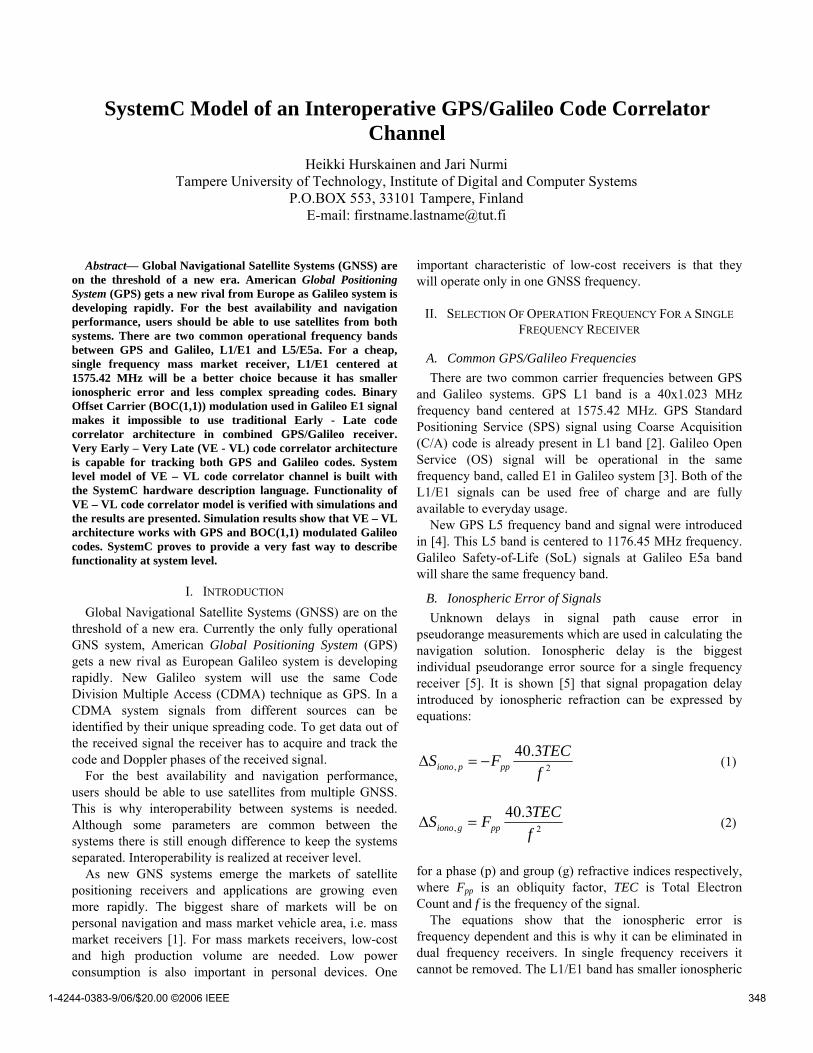
Abstract— Global Navigational Satellite Systems (GNSS) are on the threshold of a new era. American Global Positioning System (GPS) gets a new rival from Europe as Galileo system is developing rapidly. For the best availability and navigation performance, users should be able to use satellites from both systems. There are two common operational frequency bands between GPS and Galileo, L1/E1 and L5/E5a. For a cheap, single frequency mass market receiver, L1/E1 centered at 1575.42 MHz will be a better choice because it has smaller ionospheric error and less complex spreading codes. Binary Offset Carrier (BOC(1,1)) modulation used in Galileo E1 signal makes it impossible to use traditional Early - Late code correlator architecture in combined GPS/Galileo receiver. Very Early – Very Late (VE - VL) code correlator architecture is capable for tracking both GPS and Galileo codes. System level model of VE – VL code correlator channel is built with the SystemC hardware description language. Functionality of VE – VL code correlator model is verified with simulations and the results are presented. Simulation results show that VE – VL architecture works with GPS and BOC(1,1) modulated Galileo codes. SystemC proves to provide a very fast way to describe functionality at system level.
I. INTRODUCTION Global Navigational Satellite Systems (GNSS) are on the
threshold of a new era. Currently the only fully operational GNS system, American Global Positioning System (GPS) gets a new rival as European Galileo system is developing rapidly. New Galileo system will use the same Code Division Multiple Access (CDMA) technique as GPS. In a CDMA system signals from different sources can be identified by their unique spreading code. To get data out of the received signal the receiver has to acquire and track the code and Doppler phases of the received signal.
For the best availability and navigation performance, users should be able to use satellites from multiple GNSS. This is why interoperability between systems is needed. Although some parameters are common between the systems there is still enough difference to keep the systems separated. Interoperability is realized at receiver level.
As new GNS systems emerge the markets of satellite positioning receivers and applications are growing even more rapidly. The biggest share of markets will be on personal navigation and mass market vehicle area, i.e. mass market receivers [1]. For mass markets receivers, low-cost and high production volume are needed. Low power consumption is also important in personal devices. One
important characteristic of low-cost receivers is that they will operate only in one GNSS frequency.
II. SELECTION OF OPERATION FREQUENCY FOR A SINGLE FREQUENCY RECEIVER
A. Common GPS/Galileo Frequencies There are two common carrier frequencies between GPS
and Galileo systems. GPS L1 band is a 40x1.023 MHz frequency band centered at 1575.42 MHz. GPS Standard Positioning Service (SPS) signal using Coarse Acquisition (C/A) code is already present in L1 band [2]. Galileo Open Service (OS) signal will be operational in the same frequency band, called E1 in Galileo system [3]. Both of the L1/E1 signals can be used free of charge and are fully available to everyday usage.
New GPS L5 frequency band and signal were introduced in [4]. This L5 band is centered to 1176.45 MHz frequency. Galileo Safety-of-Life (SoL) signals at Galileo E5a band will share the same frequency band.
B. Ionospheric Error of Signals Unknown delays in signal path cause error in
pseudorange measurements which are used in calculating the navigation solution. Ionospheric delay is the biggest individual pseudorange error source for a single frequency receiver [5]. It is shown [5] that signal propagation delay introduced by ionospheric refraction can be expressed by equations:
2,3.40fTECFS pppiono −=∆ (1)
2,3.40fTECFS ppgiono =∆ (2)
for a phase (p) and group (g) refractive indices respectively, where Fpp is an obliquity factor, TEC is Total Electron Count and f is the frequency of the signal.
The equations show that the ionospheric error is frequency dependent and this is why it can be eliminated in dual frequency receivers. In single frequency receivers it cannot be removed. The L1/E1 band has smaller ionospheric
SystemC Model of an Interoperative GPS/Galileo Code Correlator Channel
Heikki Hurskainen and Jari Nurmi Tampere University of Technology, Institute of Digital and Computer Systems
P.O.BOX 553, 33101 Tampere, Finland E-mail: [email protected]
3481-4244-0383-9/06/$20.00 ©2006 IEEE

error than the L5/E5a band due to its higher frequency. This will make L1/E1 frequency band a more suitable selection for GPS/Galileo single frequency receivers.
C. Properties of L1/E1 and L5/E5a signals Currently the only navigation signal available for civilian
users on common GNSS frequencies is the GPS C/A signal on L1 band. It has 1023 chips long spreading code that is unique to every GPS satellite. Pseudorandom spreading codes (PRN) are Gold code [6] like sequences that are generated by two 10 chips long Linear Feedback Shift Registers (LFSR). GPS C/A PRN codes have a chiprate of 1.023 MHz so the epoch time of GPS C/A PRN code is one millisecond. Navigation data is modulated to PRN code at 50 bps. Combined data and spreading code are modulated to L1 carrier wave using Binary Phase Shift Keying (BPSK) technique.
GPS L5 signal will have separate PRN codes for the in-phase (I) and quadrature-phase (Q) of the carrier. Codes are generated with LFSR structure and are 10230 chips long. Chipping rate of GPS L5 codes is 10.23 MHz so one code epoch will last one millisecond. Navigation data is modulated at 100 bps rate to I code while Q code remains without data. [4]
In future Galileo E1 Open Service signal the PRN sequences will be 4092 chips long with 1.023 MHz chiprate. This leads to 4 ms code epoch time. Galileo PRN codes [7] and the Galileo OS Signal-in-space Interface Control Document [3] were published at the time of writing this paper. The codes are non-generatable memory codes. E1 OS signal will have two PRN codes. E1-B code at I phase of the carrier will be datamodulated with 250 symbols/s data rate and E1-C code at Q phase will be a dataless pilot with possible low rate synchronization data. The biggest difference compared to GPS C/A will be the new Binary Offset Carrier (BOC(1,1)) modulation.
Signals in Galileo E5a band are designed for SoL service. Galileo E5a signals have separate spreading codes for I and Q phase of the carrier. E5a-I and –Q codes have 10230 chips long primary codes and secondary codes are 20 chips for E5a-I and 100 chips for E5a-Q [3].
Properties of L1/E1 and L5/E5a spreading codes are summarized in Table 1. L1/E1 signals have shorter PRN codes and lower chip rates than L5/E5a signals. This makes them a better choice for receivers when lower computational burden is needed. This is the case in mass markets receivers.
III. BOC(1,1) MODULATION Binary Offset Carrier (BOC(1,1)) modulation will be used
in Galileo E1 OS signals [3]. It has also been proposed that future GPS III would use BOC(1,1) modulated signal in L1 band [8]. BOC modulated signal is created by multiplying the spreading code with a square-wave sub-carrier before modulating it with a sine wave carrier. BOC(1,1) signal has a 1.023 MHz sub-carrier and 1.023 MHz code rate.
BOC(1,1) modulation is illustrated in Fig. 1. BOC(1,1) modulation is more robust to multipath effects
and improves positioning accuracy [9]. BOC modulation creates ambiguities to the code’s autocorrelation function (ACF) and this is why traditional GPS tracking methods can not be used with BOC(1,1) modulated signals. Difference between ACFs of BPSK and BOC(1,1) modulated signals is illustrated in Fig. 2. The ACF of the BOC(1,1) modulated signal has two sidelobes on both sides of the main lobe. These sidelobes can mislead the code tracking loop, resulting in error in the pseudorange measurements used for the position calculation.
IV. DLL TRACKING Before digital signal processing the incoming signal is
down-converted and digitalized. Delay Locked Loop (DLL) is used for tracking the code phase of the received signal. The signal’s Doppler phase must also be tracked. This can be done by a Phase Locked Loop (PLL) or Frequency Locked Loop (FLL) [10] but those are out of the scope of this paper.
TABLE 1
PROPERTIES OF L1/E1 AND L5/E5A SIGNALS PRN CODES Frequency band
Signal Code size [chips]
Code rate
PRN Epoch time
GPS C/A 1023 1.023 MHz 1 ms L1/E1 1575.45 MHz Galileo
E1-B E1-C
4092 4092
1.023 MHz 1.023 MHz
4 ms 4 ms
GPS L5-I L5-Q
10230 10230
10.230 MHz 10.230 MHz
1 ms 1 ms
L5/E5a 1176.45 MHz
Galileo E5a-I E5a-Q
10230, 20a 10230, 100
10.230 MHz b 1.000 kHz c
20 ms 100 ms
a For Galileo E5a PRN codes first size is for a primary code and second for a secondary code.
b Code rate of the primary code c Code rate of the secondary code.
0 0.2 0.4 0.6 0.8 1
x 10−5
−1
0
1
time [s]
PRN
0 0.2 0.4 0.6 0.8 1
x 10−5
−1
0
1
time [s]
BOC(1,1)
0 0.2 0.4 0.6 0.8 1
x 10−5
−1
0
1
time [s]
PRN*BOC(1,1)
Fig. 1 BOC(1,1) Modulation at 1.023 MHz frequency. PRN code is on the top. BOC(1,1) subcarrier in the middle and BOC(1,1) modulated PRN at the bottom.
349

−1.5 −1 −0.5 0 0.5 1 1.5
−0.5
0
0.5
1
Ideal Autocorrelation Functions
Delay [Chips]
Nor
mal
ized
AC
F
BOC(1,1)BPSK
Fig. 2 Ideal Autocorrelation Functions of BOC(1,1) and BPSK modulated signals.
In DLL the received code is correlated with delayed
versions of the locally generated code. Discriminator functions are used to compute tracking error from the correlator outputs. Error is corrected towards zero by adjusting the code generation speed. In GPS C/A code tracking this error correction is usually made once in every millisecond (one code epoch) before data bit boundaries are found. After bit synchronization this interval is increased to 20 ms (one databit epoch). [10]
Code generation speed is controlled by a Numerically Controlled Oscillator (NCO).
A. Early—Late Correlator In current GPS C/A receivers code phase is usually
tracked with E – L correlator architecture. The incoming signal is processed and correlated with three versions of a locally generated code. One chip spacing between E and L correlators allows DLL tracking loop to determine if the phase difference between received and locally generated code is within one chip [10]. E – L correlator architecture is illustrated in Fig. 3.
Fig. 3 Early – Late code correlator architecture. I and Q phase of the incoming signal are correlated with early, prompt and late versions of a locally generated code.
B. Very Early—Very Late Correlation Fine and Wilson introduced a bump-jumping algorithm
which can be used to track BOC-modulated signals [11]. Very Early—Very Late (VE—VL) correlation uses this algorithm [12]. In VE—VL architecture additional correlators, very early and very late, are used to indicate that a wrong peak is selected. The results from these correlators are compared and if one is constantly greater than the other then a wrong peak is tracked. VE – VL architecture is illustrated in Fig. 4.
C. DLL Discriminator Functions Three common DLL discriminator functions that are used
to form the error signal from early, prompt and late correlation outputs are [5]:
Dot product
( ) ( ) PLEPLE QQQIII ×−+×− , (3) Early minus late envelope
( ) ( )2222LLEE QIQI +−+ , (4)
and Early minus late power ( ) ( )2222
LLEE QIQI +−+ . (5)
VE-VL correlator uses an additional discriminator function to determine that the correct peak is tracked. It compares VE and VL samples and if either one is constantly greater than the other it indicates that a wrong peak is tracked.
V. IMPLEMENTATION
A. Implementation Target The implementation target was to build a system level
model of a code correlator channel capable of tracking both GPS and Galileo signals on L1/E1 frequency band. These signals were chosen for implementation target because of their lower computational burden and smaller ionospheric error.
B. Implementation Language SystemC is a C/C++ class library that can be used to
create cycle-accurate models of hardware architectures. SystemC hardware description language was chosen for implementation because of its similar syntax with C++ code that enabled fast implementation without previous knowledge of hardware description languages (HDL).
A design bottleneck that follows from this decision is that the design flow after system level modeling with SystemC is not so clear as it is with other HDL’s, like VHDL and Verilog.
C. Implemented Architecture Very Early – Very Late correlator architecture (Fig. 4)
was chosen for implementation because of its ability to
350
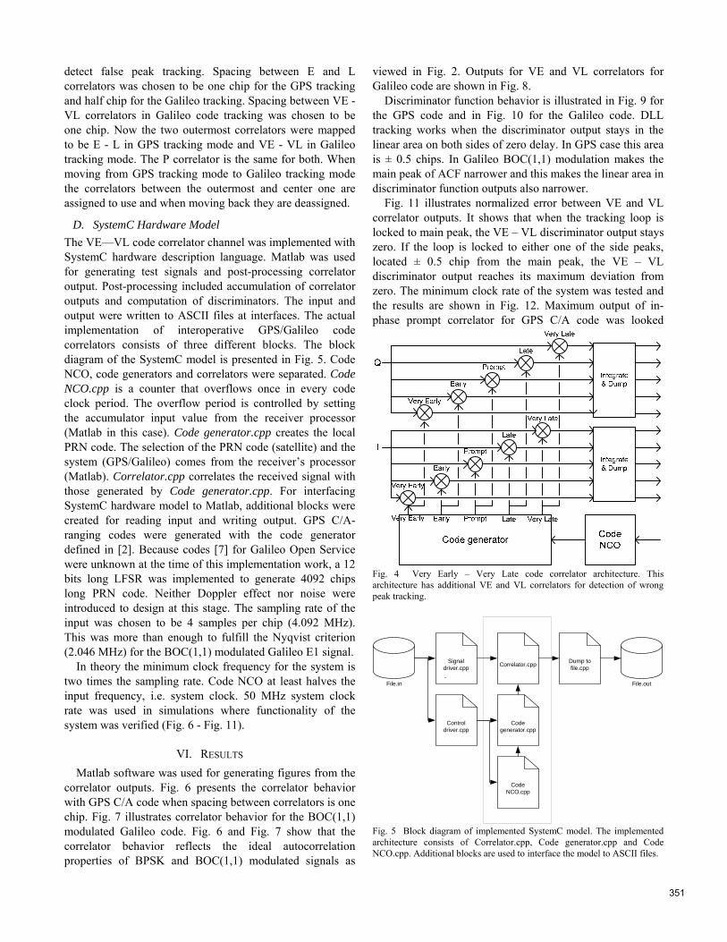
detect false peak tracking. Spacing between E and L correlators was chosen to be one chip for the GPS tracking and half chip for the Galileo tracking. Spacing between VE - VL correlators in Galileo code tracking was chosen to be one chip. Now the two outermost correlators were mapped to be E - L in GPS tracking mode and VE - VL in Galileo tracking mode. The P correlator is the same for both. When moving from GPS tracking mode to Galileo tracking mode the correlators between the outermost and center one are assigned to use and when moving back they are deassigned.
D. SystemC Hardware Model The VE—VL code correlator channel was implemented with SystemC hardware description language. Matlab was used for generating test signals and post-processing correlator output. Post-processing included accumulation of correlator outputs and computation of discriminators. The input and output were written to ASCII files at interfaces. The actual implementation of interoperative GPS/Galileo code correlators consists of three different blocks. The block diagram of the SystemC model is presented in Fig. 5. Code NCO, code generators and correlators were separated. Code NCO.cpp is a counter that overflows once in every code clock period. The overflow period is controlled by setting the accumulator input value from the receiver processor (Matlab in this case). Code generator.cpp creates the local PRN code. The selection of the PRN code (satellite) and the system (GPS/Galileo) comes from the receiver’s processor (Matlab). Correlator.cpp correlates the received signal with those generated by Code generator.cpp. For interfacing SystemC hardware model to Matlab, additional blocks were created for reading input and writing output. GPS C/A-ranging codes were generated with the code generator defined in [2]. Because codes [7] for Galileo Open Service were unknown at the time of this implementation work, a 12 bits long LFSR was implemented to generate 4092 chips long PRN code. Neither Doppler effect nor noise were introduced to design at this stage. The sampling rate of the input was chosen to be 4 samples per chip (4.092 MHz). This was more than enough to fulfill the Nyqvist criterion (2.046 MHz) for the BOC(1,1) modulated Galileo E1 signal.
In theory the minimum clock frequency for the system is two times the sampling rate. Code NCO at least halves the input frequency, i.e. system clock. 50 MHz system clock rate was used in simulations where functionality of the system was verified (Fig. 6 - Fig. 11).
VI. RESULTS Matlab software was used for generating figures from the
correlator outputs. Fig. 6 presents the correlator behavior with GPS C/A code when spacing between correlators is one chip. Fig. 7 illustrates correlator behavior for the BOC(1,1) modulated Galileo code. Fig. 6 and Fig. 7 show that the correlator behavior reflects the ideal autocorrelation properties of BPSK and BOC(1,1) modulated signals as
viewed in Fig. 2. Outputs for VE and VL correlators for Galileo code are shown in Fig. 8.
Discriminator function behavior is illustrated in Fig. 9 for the GPS code and in Fig. 10 for the Galileo code. DLL tracking works when the discriminator output stays in the linear area on both sides of zero delay. In GPS case this area is ± 0.5 chips. In Galileo BOC(1,1) modulation makes the main peak of ACF narrower and this makes the linear area in discriminator function outputs also narrower.
Fig. 11 illustrates normalized error between VE and VL correlator outputs. It shows that when the tracking loop is locked to main peak, the VE – VL discriminator output stays zero. If the loop is locked to either one of the side peaks, located ± 0.5 chip from the main peak, the VE – VL discriminator output reaches its maximum deviation from zero. The minimum clock rate of the system was tested and the results are shown in Fig. 12. Maximum output of in- phase prompt correlator for GPS C/A code was looked
Fig. 4 Very Early – Very Late code correlator architecture. This architecture has additional VE and VL correlators for detection of wrong peak tracking.
File.in
Correlator.cpp
Code generator.cpp
Code NCO.cpp
File.out
Signal driver.cpp
Dump to file.cpp
Control driver.cpp
Fig. 5 Block diagram of implemented SystemC model. The implemented architecture consists of Correlator.cpp, Code generator.cpp and Code NCO.cpp. Additional blocks are used to interface the model to ASCII files.
351
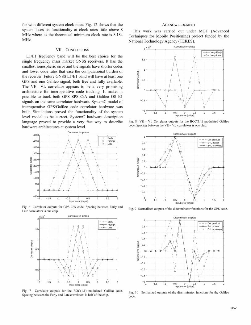
for with different system clock rates. Fig. 12 shows that the system loses its functionality at clock rates little above 8 MHz where as the theoretical minimum clock rate is 8.184 MHz.
VII. CONCLUSIONS L1/E1 frequency band will be the best choice for the
single frequency mass market GNSS receivers. It has the smallest ionospheric error and the signals have shorter codes and lower code rates that ease the computational burden of the receiver. Future GNSS L1/E1 band will have at least one GPS and one Galileo signal, both free and fully available. The VE—VL correlator appears to be a very promising architecture for interoperative code tracking. It makes it possible to track both GPS SPS C/A and Galileo OS E1 signals on the same correlator hardware. SystemC model of interoperative GPS/Galileo code correlator hardware was built. Simulations proved the functionality of the system level model to be correct. SystemC hardware description language proved to provide a very fast way to describe hardware architectures at system level.
−2 −1.5 −1 −0.5 0 0.5 1 1.5 2−500
0
500
1000
1500
2000
2500
3000
3500
4000
4500
Input error [chips]
Cor
rela
tor
outp
ut
Correlator in−phase
EarlyPromptLate
Fig. 6 Correlator outputs for GPS C/A code. Spacing between Early and Late correlators is one chip.
−2 −1.5 −1 −0.5 0 0.5 1 1.5 2−1
−0.5
0
0.5
1
1.5
2x 10
4
Input error [chips]
Cor
rela
tor
outp
ut
Correlator in−phase
EarlyPromptLate
Fig. 7 Correlator outputs for the BOC(1,1) modulated Galileo code. Spacing between the Early and Late correlators is half of the chip.
ACKNOWLEDGMENT This work was carried out under MOT (Advanced
Techniques for Mobile Positioning) project funded by the National Technology Agency (TEKES).
−2 −1.5 −1 −0.5 0 0.5 1 1.5 2−1
−0.5
0
0.5
1
1.5
2x 10
4
Input error [chips]
Cor
rela
tor
outp
ut
Correlator in−phase
Very EarlyVery Late
Fig. 8 VE – VL Correlator outputs for the BOC(1,1) modulated Galileo code. Spacing between the VE – VL correlators is one chip.
−2 −1.5 −1 −0.5 0 0.5 1 1.5 2−1
−0.8
−0.6
−0.4
−0.2
0
0.2
0.4
0.6
0.8
1
Input error [chips]
Nor
mal
ized
out
put
Discriminator outputs
Dot productE−L powerE−L envelope
Fig. 9 Normalized outputs of the discriminator functions for the GPS code.
−2 −1.5 −1 −0.5 0 0.5 1 1.5 2−1
−0.8
−0.6
−0.4
−0.2
0
0.2
0.4
0.6
0.8
1
Input error [chips]
Nor
mal
ized
out
put
Discriminator outputs
Dot productE−L powerE−L envelope
Fig. 10 Normalized outputs of the discriminator functions for the Galileo code.
352
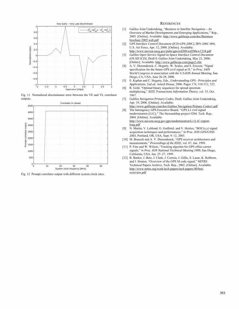
−2 −1.5 −1 −0.5 0 0.5 1 1.5 2−1
−0.8
−0.6
−0.4
−0.2
0
0.2
0.4
0.6
0.8
1
Input error [chips]
Nor
mal
ized
out
put
Very Early − Very Late discriminator
(IVE2 +Q
VE2 ) − (I
VL2 +Q
VL2 )
Fig. 11 Normalized discriminator error between the VE and VL correlator outputs.
0 10 20 30 40 500
500
1000
1500
2000
2500
3000
3500
4000
4500Correlator In−phase
Pro
mpt
cor
rela
tor
outp
ut
System clock frequency [MHz]
Fig. 12 Prompt correlator output with different system clock rates.
REFERENCES [1] Galileo Joint Undertaking, “Business in Satellite Navigation – An
Overview of Market Developments and Emerging Applications,” Rep., 2005. [Online]. Available: http://www.galileoju.com/doc/Business brochure 2005 web.pdf
[2] GPS Interface Control Document (ICD-GPS-200C), IRN-200C-004, U.S. Air Force, Apr. 12, 2000. [Online]. Available: http://www.navcen.uscg.gov/pubs/gps/icd200/icd200cw1234.pdf
[3] Galileo Open Service Signal-in-Space Interface Control Document (OS SIS ICD), Draft 0, Galileo Joint Undertaking, May 23, 2006. [Online]. Available: http://www.galileoju.com/page2.cfm
[4] A. V. Dierendonck, C. Hegarty, W. Scales, and S. Ericson, “Signal specification for the future GPS civil signal at l5,” in Proc. IAIN World Congress in association with the U.S.ION Annual Meeting, San Diego, CA, USA, June 26-28, 2000.
[5] E. Kaplan and C. Hegarty, Eds., Understanding GPS - Principles and Applications, 2nd ed. Artech House, 2006. Pages 174, 310-312, 322.
[6] R. Gold, “Optimal binary sequences for spread spectrum multiplexing,” IEEE Transactions Information Theory, vol. 33, Oct. 1967.
[7] Galileo Navigation Primary Codes, Draft, Galileo Joint Undertaking, Apr. 19, 2006. [Online]. Available: http://www.galileoju.com/doc/Galileo Navigation Primary Codes1.pdf
[8] The Interagency GPS Executive Board, “GPS L1 civil signal modernization (L1C),” The Stewardship project #204, Tech. Rep., 2004. [Online]. Available: http://www.navcen.uscg.gov/gps/modernization/L1/L1C-report-long.pdf
[9] N. Martin, V. Leblond, G. Guillotel, and V. Heiries, “BOC(x,y) signal acquisition techniques and performances,” in Proc. ION GPS/GNSS 2003, Portland, OR, USA, Sept. 9–12, 2003.
[10] M. Braasch and A. V. Dierendonck, “GPS receiver architectures and measurements,” Proceedings of the IEEE, vol. 87, Jan. 1999.
[11] P. Fine and W. Wilson, “Tracking algoritm for GPS offset carrier signals,” in Proc. ION National Technical Meeting 1999, San Diego, California, USA, Jan. 25–27, 1999.
[12] B. Barker, J. Betz, J. Clark, J. Correia, J. Gillis, S. Lazar, K. Rehborn, and J. Straton, “Overview of the GPS M code signal,” MITRE Technical Papers Archive, Tech. Rep., 2002. [Online]. Available: http://www.mitre.org/work/tech papers/tech papers 00/betz overview.pdf
353


Publication 2
c©2007 Heikki Hurskainen. Right of first publication credited to ION. Re-printed from Proceedings of the 20th International Technical Meeting of theSatellite Division of the Institute of Navigation ION GNSS 2007, “EnhancingUsability of the GRANADA Bit-True Receiver Simulation on Galileo L1” ,Heikki Hurskainen, Xuan Hu, Sireesha Ancha, Graham Bell, Jussi Raasakka,and Jari Nurmi.

Enhancing Usability of the GRANADA Bit-True Receiver Simulation on Galileo L1
Heikki Hurskainen(1), Xuan Hu(2), Sireesha Ancha(3), Graham Bell(3), Jussi Raasakka(1), and Jari Nurmi(1)
(1) Tampere University of Technology, Institute of Digital and Computer Systems, Finland (2) Tampere University of Technology, Institute of Communications Engineering, Finland
(3) PA Consulting Group, Cambridge Technology Center, UK BIOGRAPHY
Heikki Hurskainen received his M.Sc. degree in Electrical Engineering in 2005 from Tampere University of Technology, Finland. He is currently a research scientist at TUT, Institute of Digital and Computer Systems, where he works in projects on satellite navigation and is taking his post-graduate studies in the area of digital design and systems. His research interests include, but are not restricted to, current and upcoming satellite navigation systems and the simulation and implementation issues of GNSS receiver algorithms.
Xuan Hu is working towards his M.Sc. in Tampere University of Technology, Institute of Communications Engineering. He has been involved in the GREAT project since 2006. Currently he is working on algorithmic development and software implementation of the GNSS receiver.
Sireesha Ancha received her Master of Sciences (Software Systems) from the Birla Institute of Technology & Science and before that a Bachelor of Technology (Electronics and Communications Engineering) from Sri Venkateswara University, India. She joined PA in 2006 and is a member of the DSP Group within PA's Wireless Technology Practice. Sireesha is currently been involved in the GREAT project coordinating the technical architecture in the development of Mass-Market Galileo Receivers and is responsible for the technical input to the members of the consortium. Sireesha previously worked for Electronics Corporation of India Ltd in India where she was involved in the design, development and integration of digital signal processors for high speed search receiver applications, RF design and software development for wideband radio spectrum monitoring and analysis system.
Graham Bell received his M.Eng degree in Electronic and Electrical Engineering from University of Birmingham in 1996 and is currently enrolled on a part-time MBA course with the Open University. He joined the Wireless Technology Practice of PA Consulting Group where he currently holds a position as a Principal Consultant. His
focus is on technology development for wireless systems, working in four main areas: product strategy; wireless system design; terminal product development and wireless applications for clients in Europe, the US and Japan. Graham has worked on a variety of projects from feasibility through to production ready development. Graham is currently the project coordinator for the GREAT project.
Jussi Raasakka is working towards his M.Sc. in Tampere University of Technology, Institute of Digital and Computer Systems. He is currently working on a project related to GNS Systems and his research is focused on modeling parts of the GNSS receiver.
Jari Nurmi is a professor of Digital and Computer Systems at Tampere University of Technology (TUT). He has held various research, education and management positions at TUT and in the industry since 1987. He got a PhD degree from TUT in 1994. His current research interests include System-on-Chip integration, on-chip communication, embedded and application-specific processor architectures, and circuit implementations of digital communication, positioning and DSP systems. He is leading a group of about 25 researchers at TUT. Dr. Nurmi is the general chairman of the annual International Symposium on System-on-Chip (SoC) and its predecessor SoC Seminar in Tampere since 1999, and a board member of SoC, FPL, and NORCHIP conference series. He was the head of the national TELESOC graduate school 2001-2005. He is the author or co-author of about 160 international papers, editor of Springer book “Processor Design: System-on-Chip Computing for ASICs and FPGAs,” co-editor of Kluwer book “Interconnect-centric design for advanced SoC and NoC”, and has supervised more than 90 MSc, Licentiate and Doctoral theses. He is a senior member in IEEE Signal Processing Society, Circuits and Systems Society, Computer Society, Solid-State Circuits Society and Communications Society. In 2004, he was one of the recipients of Nokia Educational Award, and the recipient of Tampere Congress Award 2005. He has been awarded one of the Academy of Finland Senior Scientist research grants for the academic year 2007-2008.
2707

ABSTRACT
Simulation and simulation tools perform an essential role in the research and development of new satellite navigation systems, such as Galileo. Within the Galileo research community there have not been any standardized tools for simulation and the researchers have been forced to build their own proprietary tools to carry out simulations. A tool called GRANADA was developed by Deimos-Space in the GARDA (GAlileo Receiver Development Activities) project and it has become quite popular among the Galileo researchers.
GRANADA consists of two complementary tools. The Bit-True GNSS Receiver Simulator is a tool built in the Simulink environment which models the navigation signal processing chain consisting of the transmitter, propagation channel and Galileo receiver blocks. The receiver tool is modular and configurable and it has been successfully used in several documented studies. The other tool in GRANADA is the GNSS Environment and Navigation Simulator but it is out of the scope of this paper.
In our project, called GREAT (Galileo REceiver for mAss markeT), we are using GRANADA as one of the implementation and testing platforms for studying multipath mitigation and advanced tracking algorithms. The purpose of this paper is to present the customization work we have done to enhance the GRANADA Bit-True GNSS Receiver Simulator v2.02 to make it more suitable for our needs. In particular we have addressed the issues of repeatability of simulation runs; synchronization between acquisition and tracking units; and modifications to align the simulation results with theoretical ones.
We conclude that GRANADA is a tool with high potential for Galileo research and it is becoming more widely used in the Galileo research community. We believe that the steps towards enhancement of usability presented in this paper will also benefit the other researchers who are using the GRANADA tool.
This work was carried out under GREAT project, co-funded by the European GNSS Supervisory Authority (GSA) with funding from the 6th Framework Programme of the European Community for research and technological development.
INTRODUCTION
Simulation and the simulation tools play an essential role in the analysis, design, test, and verification stages in research and development of a new satellite navigation system. The European Galileo system, currently under development, will complement the existing Navstar Global Positioning System (GPS). Together these two systems will form the foundations of near future Global Navigational Satellite System (GNSS).
Within the Galileo research community there have not been any standardized tools for simulation. Researchers have been forced to build their own proprietary tools to carry out simulations. This makes it difficult, or even impossible, to compare the results acquired from different studies. Lately, a tool called GRANADA (Galileo Receiver ANAlysis and Design Application) [1] has become quite popular among the Galileo researcher community. GRANADA was developed by Deimos-Space in the GARDA (GAlileo Receiver Development Activities) project. The GARDA project was funded from European Union 6th Frame Program funds and managed by the Galileo Joint Undertaking (GJU).
The GREAT (Galileo REceiver for mAss markeT) project is another EU 6 FP funded project, currently managed by the European GNSS Supervisory Authority (GSA). One of the GREAT project objectives is to study multipath mitigation and advanced tracking algorithms.
The purpose of this paper is to present the customization work we, in the GREAT project, have done to enhance the GRANADA Bit-True GNSS Receiver Simulator v2.02 to make it more suitable for our needs in research of multipath mitigation and advanced tracking algorithms. At first, we will familiarise the reader with the GRANADA software. The overview of the software and how it has been used in earlier studies will be given with a literature review. Then we discuss the role of GRANADA in the GREAT project and give a detailed view of the enhancements we have done to the software.
To authors’ knowledge the enhancements presented in this paper are not issued in any of the earlier publications concerning GRANADA software and simulations. The presented work is significant to the GREAT project because it allows us to build a uniform testing platform for our further research. We strongly believe that the presented work also benefits all the fellow researchers working with the GRANADA tools.
BACKGROUND & MOTIVATION
In this section we give an overview of the GRANADA software and to how it has been used in different studies. The role of GRANADA software in the GREAT project is also discussed.
GRANADA consists of two complementary tools [2]. The Bit-True GNSS Receiver Simulator is a tool built in the Simulink environment which models the navigation signal processing chain. This consists of the transmitter, propagation channel and Galileo receiver blocks, illustrated in Figure 1. The receiver tool is modular and it can be configured easily through the graphical user interface (GUI). The other tool in GRANADA is the GNSS Environment and Navigation Simulator but this is out of the scope of this paper and henceforth “the software” refers only to the GRANADA Bit-True GNSS
2708

Receiver Simulator. In last years GRANADA has been widely accepted as a de facto tool for Galileo research by multiple research communities.
Figure 1: A screenshot from GRANADA Bit-True GNSS Receiver Simulator showing its three main blocks: Galileo transmitter, Propagation channel, and Galileo receiver.
When measured in terms of published material, the main users of the software have been the researchers in GARDA project. GRANADA has been used to measure the Galileo receiver’s performance under other GPS interference and multipath conditions [1], to validate the novel BOC tracking technique [3], and to analyze the code Doppler shifts on Galileo E5 and L1 OS signals [4]. The software simulator’s role as a key element in the GARDA project was discussed in a wide journal article [5]. In another article by different authors [6], the GRANADA software’s role in teaching and algorithm test-benching was mentioned briefly.
In the GREAT project, one of our objectives has been to analyze and implement algorithms for multipath mitigation and advanced tracking for Galileo L1 Open Service signals. Some of these results are already published in [7]. The GRANADA software’s role in our project is to be one of the common implementation and testing platforms between the project members, and it has been used as such e.g. to validate the studied tracking algorithms [8].
ENHANCING USABILITY
In this section we introduce the modification work that we have done to enhance the software to fit in our needs. In particular we have addressed the issues of repeatability of simulation runs, synchronization between acquisition and tracking units and modifications to align the simulation results with theory in the generation of Multipath Error Envelopes (MEEs).
The version we used was GRANADA Bit True Simulator v2.02 and the repeatability issues were studied only for simulations concerning Galileo L1 OS signals.
Repeatability of the GRANADA simulation runs
Repeatability is an important property of any research performed. In principle, it should be possible to create a test setup and repeat documented research with documented tools so that the result remains the same to bit-exact accuracy when the input and the simulation environment have not been changed.
In the original (v2.02) version of the GRANADA Bit-True GNSS Receiver Simulator tool some of its features cause variation in the results between simulation runs, even if the input and configuration parameters remain unchanged.
In the next section we discuss the architecture of the tool and identify the sources of these result variations. We also discuss how to customize the Bit-True GNSS Receiver Simulator so that the simulation results can be repeated. Simulation results are presented to illustrate the effects of non-repeatability and to verify the repeatability of the simulations made with the customized tool.
GRANADA BT GNSS Receiver Simulator architecture and operation modes
GRANADA BT consists of the transmitter model, channel model and Galileo receiver model. The basic operation modes are the intermediate frequency (IF) model and the passband model where carrier IF is neglected. The models can be executed as either on-the-fly or offline modes. [2]
When running an on-the-fly simulation, the input is generated, channel is processed and signal is received in parallel processes. In the offline processing mode the input is read from an input file located on a user’s hard drive. This file is generated and saved before simulation. The offline input file can be saved (and then loaded) either before or after the propagation channel model.
The Galileo receiver model receives the signal with user defined channel effects; including multipath, GPS and external interferences. The receiver outputs several parameters describing the behavior of the received signal and the receiver operations. These parameters include bit error rate (BER), tracking loop behavior (Delay-, Frequency-, and Phase Locked Loop) etc.
The user can configure the input parameters for each simulation through the GUI. The configurations can be saved to a file and loaded from there for a new simulation, thus allowing an easy import of simulation input and configuration into a new simulation run. The user definable parameters include many transmitter, propagation channel, receiver IF and baseband component
2709

characteristics. One very important parameter modification from a repeatability point of view is changing the incoming code delay from a random value (default) to a constant one.
In our multipath mitigation and advanced tracking algorithm studies, we were mostly interested in tracking loop output parameters, as they reflect the behavior of the tracking algorithms. During our work we faced some difficulties in comparing the behavior of the algorithms since the studied parameters were changing even if the model was executed again with the exactly same input and configuration parameters. In some studies randomness may be a desired effect but in our case it was not wanted.
A tool for output comparison
We developed a tool for testing the equality of the output parameters from different simulation runs. The tool is a Matlab script that reads the output parameters (Matlab workspace variables) from two user defined simulation output files and simply compares them, resulting in the output string “equal” or “not equal”. An example of the comparison tool’s output (only the seven first variables from the start) is given in Table 1. With this tool we started to go through the GRANADA BT GNSS receiver simulator to identify the reasons for variance between outputs of separate simulation runs.
When running the simulator twice consecutively with the same input configuration and then comparing the equality of the outputs, we were getting from 12 to 16 “not equal” variables out of a total 145, depending on the simulation type. The comparison number differs a little with different simulation configurations (usage of GPS interference, PLL/FLL, etc.) but in general the output parameters that we were interested in - the Bit Error Rate and active tracking loop outputs (DLL, PLL, and FLL) - were never equal in two simulation runs with exactly the same input and configuration.
TABLE 1: EXAMPLE OF COMPARISON TOOL’S OUTPUT TEXT. 138 LINES OF COMPARISON RESULTS ARE LEFT
OUT FOR CLARITY. Source File: GranadaBTOut-L1B-070207_0857.mat Target File:GranadaBTOut-L1B-070207_0853.mat ------------------------------------- Variable :: ADC_gain || equal Variable :: AceEnd || equal Variable :: AceIni || equal Variable :: AceUser || equal Variable :: Acqflag || equal Variable :: AltBOC_mtx || equal Variable :: BER || not equal
Not shown 138 lines of comparison…
Removal of the difference in the simulation run outputs
We managed to locate the sources of these differences in simulation outputs. What we found out was that the variations in the results were a sum of many random behaviors in the model. The first step towards repeatability was to modify the obvious blocks containing random effects in the software. The propagation channel block in GRANADA BT simulator contains several sub-blocks for additive white Gaussian noise (AWGN) generation. We located these blocks and changed the random source’s seed number to a constant value. Next thing that we noticed was the randomness in phase offset of the IF carrier generation and wipe-off processes. We changed the phase offset to be a constant in both transmitter and receiver blocks.
With these modifications the GRANADA model simulation runs proved to be repeatable, as long as the simulator software was not shutdown between simulation runs. From this behavior we made a conclusion that some of the variables used by the GRANADA software are generated randomly in the initialization step of the software.
For Galileo OS L1 simulations one randomly initialized variable proved to be the L1-A signal component. Since it is not used in the receiver part but only to model the entire signal in space, we decided to substitute the L1-A code and data input parameters with a predefined constant. To make the change permanent, this substitution must be done in the Simulink model file that contains the transmitter models for all transmitters. The same kind of substitution must be done to GPS transmitter model also if repeatable simulations, with GPS interference enabled, are desired.
With all these modifications applied to the software and using exactly the same simulation configuration parameters, we managed to get the number of “not equal” output variables down to seven out of 145, in comparing two different simulation runs. A closer look with the software’s interface control document [9] connected all of these “not equal” parameters either to simulation execution time (when simulation was executed, never equal in consecutive simulation runs) or to those that were disconnected from the model (Galileo L1-A and GPS code and data generation) and thus not used in simulation.
An example output comparison of two simulation runs with both using the original and the modified versions of the software is illustrated in Figure 2 for the carrier phase error (i.e. PLL output) parameter and in Figure 3 for the code phase error (i.e. DLL output) parameter. The figures show how the tracking loop outputs from two simulation runs using the original software, with identical input and configurations, are not equal (i.e. the absolute value of the calculated difference is not equal to zero). On the other
2710

hand, the simulated tracking loop outputs achieved from simulation runs using the modified software proved to be equal (i.e. the calculated difference resulted in zero).
0 0.1 0.2 0.3 0.4 0.5 0.6 0.7 0.8 0.9 10
10
20
30
40
50
60
70
80
time (s)
Abs
olut
e di
ffere
nce
in c
arrie
r pha
se e
rror o
utpu
t (cm
)
Comparison of outputs from original and modified software
original: ∆data
original: ∆pilot
modified: ∆data
modified: ∆pilot
Figure 2: Comparison of outputs from simulations made with original and modified version of the software. The absolute difference of carrier phase error (PLL output) in simulations made with original version is displayed with magenta-circled curve for data and blue-squared for pilot. The carrier phase error output difference of modified software is illustrated in red-starred for data and black-plain for pilot.
0 0.1 0.2 0.3 0.4 0.5 0.6 0.7 0.8 0.9 10
2
4
6
8
10
12
14
16
time (s)
Abs
olut
e di
ffere
nce
in c
ode
phas
e er
ror o
utpu
t (m
)
Comparison of outputs from original and modified software
original: ∆data
original: ∆pilot
modified: ∆data
modified: ∆pilot
Figure 3: Comparison of outputs from simulations made with original and modified version of the software. The absolute difference of code phase error (DLL output) in simulations made with original version is displayed with magenta-circled curve for data and blue-squared for pilot. The code phase error output difference of modified software is illustrated in red-starred for data and black-plain for pilot.
Synchronization delay error
The other issue we faced during the work was the synchronization issue. In the original version of GRANADA, acquisition and tracking units are synchronized by using a fixed offset. This offset is used
for aligning the successful acquisition result with the prompt tracking delay. The used synchronization method causes also an offset into the estimated delays, which causes problems further down in the processing chain leading to incorrect receiver output. In this section we present the steps to be taken to cope with this.
In the Simulink model of GRANADA, the delay of the signal originates from the delay of transmission filter, the delay in the channel, the delay in receiver filter and the delay error from the Simulink itself. At first, the signal enters the acquisition stage, and the delay estimation that comes from this stage is approximately -146 meters. This delay estimation is not equal to the actual total delay caused by the propagation channel, transmitter and receiver filters. And it cannot be changed, even the acquisition time changes. However, with the default sampling rate, transmitter filter type, receiver filter type and constant initial delay offset defined in the front end of the receiver, the total signal delay, including the delay error from the Simulink itself, is fixed quite close to the estimated one, and it can roughly compensate the total signal delay. After the acquisition stage, the signal enters the tracking stage, and the delay estimation comes from the tracking unit of GRANADA BT simulator.
We can cancel this delay error by making a simulation with a noiseless, single path signal at first. Then we run the simulation for different channel profile or for different tracking algorithm. Now the delay estimation value from the noiseless and single path simulation can be considered to be the true delay of the Line-of-Sight (LOS) signal, and used as the reference. The tracking delay error is then the difference between the reference and the delay estimation coming from the DLL. Since the signal delay is fixed, the subtraction of two estimations also cancels the delay error caused by the total signal delay, and is the delay error caused by the multipath effect and noise. Figure 4 shows an example of the delay estimation in a multipath AWGN channel, and the reference true delay value.
Figure 4: An example of the GRANADA delay estimation. Red dashed line presents the reference delay and the blue solid line is the simulation output.
2711
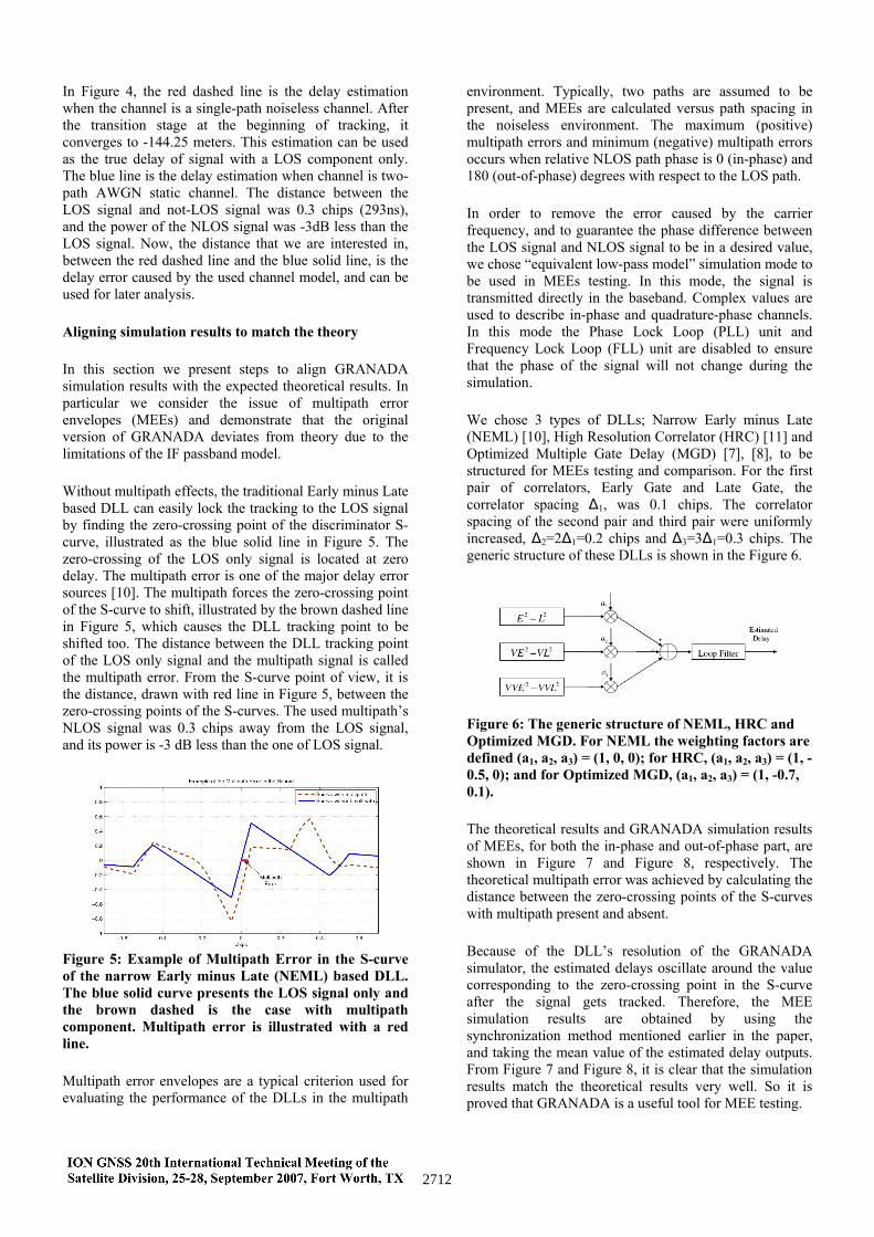
In Figure 4, the red dashed line is the delay estimation when the channel is a single-path noiseless channel. After the transition stage at the beginning of tracking, it converges to -144.25 meters. This estimation can be used as the true delay of signal with a LOS component only. The blue line is the delay estimation when channel is two-path AWGN static channel. The distance between the LOS signal and not-LOS signal was 0.3 chips (293ns), and the power of the NLOS signal was -3dB less than the LOS signal. Now, the distance that we are interested in, between the red dashed line and the blue solid line, is the delay error caused by the used channel model, and can be used for later analysis.
Aligning simulation results to match the theory
In this section we present steps to align GRANADA simulation results with the expected theoretical results. In particular we consider the issue of multipath error envelopes (MEEs) and demonstrate that the original version of GRANADA deviates from theory due to the limitations of the IF passband model.
Without multipath effects, the traditional Early minus Late based DLL can easily lock the tracking to the LOS signal by finding the zero-crossing point of the discriminator S-curve, illustrated as the blue solid line in Figure 5. The zero-crossing of the LOS only signal is located at zero delay. The multipath error is one of the major delay error sources [10]. The multipath forces the zero-crossing point of the S-curve to shift, illustrated by the brown dashed line in Figure 5, which causes the DLL tracking point to be shifted too. The distance between the DLL tracking point of the LOS only signal and the multipath signal is called the multipath error. From the S-curve point of view, it is the distance, drawn with red line in Figure 5, between the zero-crossing points of the S-curves. The used multipath’s NLOS signal was 0.3 chips away from the LOS signal, and its power is -3 dB less than the one of LOS signal.
Figure 5: Example of Multipath Error in the S-curve of the narrow Early minus Late (NEML) based DLL. The blue solid curve presents the LOS signal only and the brown dashed is the case with multipath component. Multipath error is illustrated with a red line.
Multipath error envelopes are a typical criterion used for evaluating the performance of the DLLs in the multipath
environment. Typically, two paths are assumed to be present, and MEEs are calculated versus path spacing in the noiseless environment. The maximum (positive) multipath errors and minimum (negative) multipath errors occurs when relative NLOS path phase is 0 (in-phase) and 180 (out-of-phase) degrees with respect to the LOS path.
In order to remove the error caused by the carrier frequency, and to guarantee the phase difference between the LOS signal and NLOS signal to be in a desired value, we chose “equivalent low-pass model” simulation mode to be used in MEEs testing. In this mode, the signal is transmitted directly in the baseband. Complex values are used to describe in-phase and quadrature-phase channels. In this mode the Phase Lock Loop (PLL) unit and Frequency Lock Loop (FLL) unit are disabled to ensure that the phase of the signal will not change during the simulation.
We chose 3 types of DLLs; Narrow Early minus Late (NEML) [10], High Resolution Correlator (HRC) [11] and Optimized Multiple Gate Delay (MGD) [7], [8], to be structured for MEEs testing and comparison. For the first pair of correlators, Early Gate and Late Gate, the correlator spacing ∆1, was 0.1 chips. The correlator spacing of the second pair and third pair were uniformly increased, ∆2=2∆1=0.2 chips and ∆3=3∆1=0.3 chips. The generic structure of these DLLs is shown in the Figure 6.
Figure 6: The generic structure of NEML, HRC and Optimized MGD. For NEML the weighting factors are defined (a1, a2, a3) = (1, 0, 0); for HRC, (a1, a2, a3) = (1, -0.5, 0); and for Optimized MGD, (a1, a2, a3) = (1, -0.7, 0.1).
The theoretical results and GRANADA simulation results of MEEs, for both the in-phase and out-of-phase part, are shown in Figure 7 and Figure 8, respectively. The theoretical multipath error was achieved by calculating the distance between the zero-crossing points of the S-curves with multipath present and absent.
Because of the DLL’s resolution of the GRANADA simulator, the estimated delays oscillate around the value corresponding to the zero-crossing point in the S-curve after the signal gets tracked. Therefore, the MEE simulation results are obtained by using the synchronization method mentioned earlier in the paper, and taking the mean value of the estimated delay outputs. From Figure 7 and Figure 8, it is clear that the simulation results match the theoretical results very well. So it is proved that GRANADA is a useful tool for MEE testing.
2712

Figure 7: MEE (in-phase part) comparison between the theoretical results and GRANADA simulation results. NEML is illustrated as blue solid line and circles, HRC as red dashed line and crosses, and Optimized MGD as green dashed line and triangles.
Figure 8: MEEs (out-of-phase part) comparison between the theoretical results and GRANADA simulation results. NEML is illustrated as blue solid line and circles, HRC as red dashed line and crosses, and Optimized MGD as green dashed line and triangles.
CONCLUSIONS
We conclude that GRANADA is tool with high potential for Galileo research and it is increasingly widely used in the Galileo research community. In this paper the means to make the GRANADA Bit-True GNSS Receiver Simulator runs repeatable on Galileo L1 band are discussed and the simulation results to verify this are presented.
The issue of synchronization between acquisition and tracking is discussed. The effects of this behavior and the steps on how to cope with it are also shown. A method to match the simulator results with the expected theoretical ones is explained. GRANADA is proved as a tool capable for MEE testing.
The work presented in this paper is significant to the GREAT project because it allows us to build a uniform testing platform for our further research. We strongly believe that the presented work will also benefit the other researchers who are using the GRANADA tool.
ACKNOWLEDGMENTS
This work was carried out under GREAT (Galileo Receiver for mAss markeT) project, co-funded by the European GNSS Supervisory Authority (GSA) with funding from the 6th Framework Programme of the European Community for research and technological development.
The authors also want to express their thanks to Nick Thorn from PA Consulting Group, for his effort to improve the language.
REFERENCES
[1] Fernandez, A; Diez, J; Marradi, L and Gabaglio, V. “Galileo Receiver Performance Under GPS Interference and Multipath With the GRANADA Software Receiver.” In proceedings of the ION GNSS 2004, pp. 1027–1034. Sep. 21–24, 2004. Long Beach, CA.
[2] Deimos-Space. GRANADA Software User Manual. GARDA-DMS-SUM-001. Issue 2.0. Jun. 10. 2005.
[3] de Castro, D; Diez, J; Fernadez, A and Sleewaegen, J-M. “A New Unambiguous Low-Complexity BOC Tracking Technique.” In proceedings of the ION GNSS 2006. pp. 1830–1835. Sep. 26–29, 2006. Fort Worth, TX.
[4] Diez, J; Fernández, A; Fossati, D; Marradi, L and Gabaglio, V. “Using the GRANADA Bit-True Simulator to analyse the effect of Code Doppler shift in Galileo E5 and L1 Receivers.” ENC GNSS 2005. Munich, Germany. 19-22 Jul. 2005.
[5] Marradi, L; Franzoni, G; Foglia, L; Fossati, D; Cornacchini, C; le Coff, M; Duchesne, L; Foged, L; Fernandez, A; Caramagno, A; Schwikert, R; Woerz, T; Gabaglio, V. “The GARDA Project – Building a Galileo receiver”, Inside GNSS, pp 40-52, Nov/Dec 2006.
[6] J. Won, T. Pany, and G. Hein, “GNSS software defined radio: real receiver or just a tool for experts,” Inside GNSS, pp. 48–56, Jul/Aug 2006.
[7] D. Skournetou and E. Lohan, “Non-coherent multiple correlator delay structures and their tracking performance for Galileo signals,” in ENC GNSS, 2007. May 29-Jun 1, 2007. Geneva, Switzerland.
[8] Hu, X and Lohan, E-S. “GRANADA validation of optimized Multiple Gate Delay structures for Galileo SinBOC(1,1) signal tracking.” In 7th International Conference on ITS Telecommunications. 2007. Jun. 6-8, 2007. Sophia Antipolis, France.
2713

[9] Deimos-Space. GRANADA Interface Control Document (ICD). Issue 4.0. Jun. 30. 2005. GARDA-DMS-ICD-001.
[10] Braasch, M. S. ”GPS multipath model validation” Position Location and Navigation Symposium, IEEE 1996 .pp. 672 – 678. 22-26 Apr. 1996.
[11] McGraw, A. and Braasch, M. S. “GNSS Multipath Mitigation Using Gated and High Resolution Correlator Concepts”. In proceedings of the ION NTM 1999. pp. 333–342. Jan. 25-27, 1999, San Diego, CA.
2714


Publication 3
c©2008 Heikki Hurskainen et al. Reprinted from International Journal of Na-vigation and Observation, vol. 2008, “Multiple Gate Delay Tracking Struc-tures for GNSS Signals and Their Evaluation with Simulink, SystemC andVHDL” , Heikki Hurskainen, Elena-Simona Lohan, Xuan Hu, Jussi Raa-sakka, and Jari Nurmi.

Hindawi Publishing CorporationInternational Journal of Navigation and ObservationVolume 2008, Article ID 785695, 17 pagesdoi:10.1155/2008/785695
Research ArticleMultiple Gate Delay Tracking Structures for GNSS Signals andTheir Evaluation with Simulink, SystemC, and VHDL
Heikki Hurskainen,1 Elena Simona Lohan,2 Xuan Hu,2 Jussi Raasakka,1 and Jari Nurmi1
1 Department of Computer Systems, Tampere University of Technology, P.O. Box 553, 33101 Tampere, Finland2 Department of Communications Engineering, Tampere University of Technology, P.O. Box 553, 33101 Tampere, Finland
Correspondence should be addressed to Heikki Hurskainen, [email protected]
Received 13 July 2007; Revised 11 December 2007; Accepted 29 February 2008
Recommended by Letizia Presti
Accurate delay tracking in multipath environments is one of the prerequisites of modern GNSS receivers. Several solutions havebeen proposed in the literature, both feedback and feedforward. However, this topic is still under active research focus, especiallyfor mass-market receivers, where selection of lowcomplexity, nonpatented methods is preferred. Among the most encountereddelay tracking structures implemented in today’s receivers, we have the narrow correlator and the double-delta correlators. Bothare heavily covered by various patents. The purpose of this paper is to introduce a new, generic structure, called multiple gate delay(MGD) structure, which covers also the patented correlators but offers much more flexibility in the design process. We show howthe design parameters of such a structure can be optimized, we argue the performance of this structure via detailed simulationresults based on various simulators, such as Matlab/Simulink-based tool, GRANADA, and we test the implementation feasibilityof MGD structures on actual devices, via SystemC and FPGA prototyping. One of the main advantages of the proposed structureis its high degree of flexibility, which allows the designer to choose among, to the authors’ knowledge, nonpatented solutions withdelay tracking accuracy comparable with that of the current state-of-art trackers.
Copyright © 2008 Heikki Hurskainen et al. This is an open access article distributed under the Creative Commons AttributionLicense, which permits unrestricted use, distribution, and reproduction in any medium, provided the original work is properlycited.
1. BACKGROUND AND MOTIVATION
The main algorithms used nowadays for GPS and Galileocode tracking are based on what is typically called a feedbackdelay estimator, and they are implemented based on a feed-back loop. The most known feedback delay estimators are thedelay locked loops (DLLs) and the today’s GNSS receiver thattypically use a particular DLL structure, called the narrowcorrelator or narrow early-minus-late (NEML) delay tracker,which proved to give good results in multipath environments[1–3]. Another class of enhanced DLL structures is the so-called double-delta correlator class [4], which started to gainmore and more attention during last years. Examples belong-ing to this class are: the high resolution correlator (HRC)[3, 5], the strobe correlator [2, 4, 6], the pulse aperturecorrelator (PAC) [7], the multipath mitigation correlator[8], and the modified correlator reference waveform [2, 9].Most of the double-delta correlators as well as the narrowcorrelator are patented or under patent applications [4, 5, 7,10, 11].
An alternative to the above-mentioned feedback loopsolutions is based on the open-loop (or feedforward)solutions, which refer to the solutions which make the delayestimation in a single step, without requiring a feedback loop.A general classification of open-loop solutions for CDMAcommunication applications can be found in [12, 13] and forGNSS applications in [14]. However, for the purpose of low-cost mass-market receiver implementation, feedback delaytracking structures are still the preferred ones, and they willbe the focus of our paper.
We introduce here the flexible multiple gate delay (MGD)structure with adjustable parameters, and we present amethod to optimize these parameters. We show the per-formance of MGD structures in multipath channels, witha particular attention to the situations with more than 2paths (which are typically neglected in the literature, whenanalyzing the multipath error envelopes of delay trackingunits). We also present, for the first time to the authors’knowledge, a comparison between using squared-envelopesversus envelopes before noncoherent integration stage as well

2 International Journal of Navigation and Observation
as a comparison between using uniform versus nonuniformgate spacings in delay tracking units.
We then validate the MGD structures via implementationin a Simulink-based navigation tool, GRANADA. Based onthe presented MGD structures, we also develop a flexibledelay tracking prototype receiver (in SystemC and VHDL)for Galileo and GPS signals. The main focus is on sine-BOCand BPSK-modulated signals, but the design steps shownhere can be extended in a straightforward manner to otherBOC modulations (cosine BOC, multiplexed BOC, alternateBOC, etc.).
In the delay tracking receiver prototyping, we focuson the implementability, complexity, and flexibility of theproposed MGD structures. First, we present the implemen-tations and discuss about the flexibility and the restrictionscaused mostly by the digital hardware characteristics. Then,we verify the implementability of the chosen algorithmswith a SystemC model. After that, the complexity of theimplemented prototype hardware is evaluated as VHDLsynthesis results.
2. COMMON DELAY TRACKING STRUCTURES FORGNSS SIGNALS
The most common delay tracking loops for GNSS signals arebased on feedback delay locked loop (DLL)-like structures.The state-of-art delay trackers, which are widely used inGNSS industry nowadays, include: the narrow early-minus-late (NEML) correlator [1–3, 10, 11] and the double-deltacorrelators [2, 15–17], also known under the names of pulseaperture correlator (PAC) [7], strobe correlator [2, 6, 18], orhigh resolution correlator (HRC) [3, 5, 19].
All the above-mentioned methods have a commonunderlying structure, in the sense that they are based ondifferent weighted combinations of early and late samplesof the correlation function with different chip-spacingsbetween these samples. In what follows, we will first intro-duce the signal model for Galileo and GPS signals, then, wepresent the above-mentioned methods in more detail. Wewill then show that most of the currently used delay trackingstructures (i.e., those mentioned above) can be unified undera generic structure, namely the multiple gate delay (MGD)structure, whose parameters are to be optimized in Section 3.
Typical satellite positioning signals, such as those usedfor GPS and Galileo, employ the direct-sequence codedivision multiple access (DS-CDMA) technique, where aPRN code is spreading the navigation data over SF chips(or over a code epoch length) [20, 21]. In what follows, weadopt, for clarity reasons, a baseband model. Also, the delaytracking estimation in nowadays receivers is typically donein digital domain (using the baseband correlation samples).The time notation t stands for discrete time. The transmittedsignal x(t) can be written as the convolution between themodulating waveform smod(t), the PRN code, including datamodulation, and the pulse shaping filter pTB (t) [22]:
x(t) =√Ebsmod(t)
�+∞∑
n=−∞
SF∑
k=1
bnck,nδ(t − nTsym − kTc
)� pTB (t),
(1)
where Eb is the data bit energy, � is the convolution operator,bn is the nth complex data symbol, Tc = 1/ fc is the chipperiod, SF is the spreading factor, Tsym is the symbol period(Tsym = SFTc), ck,n is the kth chip corresponding to thenth symbol, δ(t) is the Dirac pulse, and pTB (t) is the pulseshaping filter applied to pulses of durationTB = Tc/NB . Here,NB is a modulation-related parameter that is detailed in whatfollows. For example, if infinite bandwidth is assumed, pTB (t)is a rectangular pulse of unit amplitude if 0 ≤ t ≤ TB and 0otherwise.
The signal x(t) is typically transmitted over a multipathstatic or fading channel, where all interference sources(except the multipaths) are lumped into a single additiveGaussian noise term η(t):
r(t) =L∑
l=1
αle− jθl x
(t − τl
)e− j2π fDt + η(t), (2)
where r(t) is the received signal, L is the number of channelpaths, αl is the amplitude coefficient of the lth path, θl is thephase of the lth path, τl is the channel delay introduced by thelth path, fD is the Doppler shift introduced by the channel,and η(t) is the complex additive Gaussian noise of zero meanand double-sided power spectral density N0.
Typically, the signal-to-noise ratios for GNSS signalsare expressed with respect to the code epoch bandwidthBw, under the name of carrier-to-noise ratio (CNR). Therelationship between CNR and bit-energy-to-noise ratio is[23]
CNR[dB-Hz] = EbN0
+ 10log10
(Bw). (3)
The delay tracking is typically based on the code epoch-by-code epoch correlation R(·) between the incoming signaland the reference xref(·) modulated PRN code, with a certaincandidate Doppler frequency fD and delay τ:
R(τ, fD,m
) = E(
1Tsym
∫ mTsym
(m−1)Tsym
r(t)xref(τ, fD
)dt)
, (4)
where m is the code epoch index, and E(·) is the expectationoperation, with respect to the PRN code, and
xref(τ, fD
)
=(smod(t) �
+∞∑n=−∞
SF∑
k=1
bnck,nδ(t− nTsym− kTc
)�pTB (t)
)
× e+ j2π fDt,(5)
where bn are the estimated data bits. For Galileo signals, aseparate pilot channel is transmitted, thus the data bits areknown at the receiver [21]. In order to reduce the noiselevel, we can use coherent and/or noncoherent integration.
The averaged coherent correlation function Rc(τ, fD) can bewritten as
Rc(τ, fD
) = 1Nc
Nc∑
m=1
R(τ, fD,m
), (6)

Heikki Hurskainen et al. 3
where Nc is the coherent integration time (expressed in codeepochs or milliseconds for GPS/Galileo signals), and the
averaged noncoherent correlation function Rnc(τ, fD) can bewritten as
Rnc(τ, fD
) = 1Nnc
∑
Nnc
∣∣∣∣∣1Nc
Nc∑
m=1
R(τ, fD,m
)∣∣∣∣∣
pownc
, (7)
where Nnc is the noncoherent integration time, expressed inblocks of length Nc milliseconds (for clarity of presentation,we dropped the block indexes used in the noncoherent sum-mation), and pownc is a power index used for noncoherentsummation. The most encountered variants are: pownc = 1(i.e., sum of absolute values) and pownc = 2 (i.e., sum ofsquared-absolute values).
The DLL-like structures form a discriminator functionD(τ) based on the early and late correlations, and theyestimate the channel first path delay from the zero crossingsof this discriminator function. The discriminator functionsfor NEML [1–3, 10, 11] and HRC [3, 5, 19] are well defined inliterature and their expressions as equations are, for NEML:
D(τ) =Rc/nc
(τ +
Δ1
2, fD
)−Rc/nc
(τ − Δ1
2, fD
), (8)
and for HRC:
D(τ) = a1
(Rc/nc
(τ +
Δ1
2, fD
)−Rc/nc
(τ − Δ1
2, fD
))
+ a2
(Rc/nc
(τ +
Δ2
2, fD
)−Rc/nc
(τ − Δ2
2, fD
)).
(9)
In single-path channels (L = 1), the mentioned dis-criminator functions cross the zero level when τ = τ1.That is, the zero-crossings show the presence of a channelpath. However, due to BOC modulation, we might havemore zero-crossings present, and the search range should berestricted to the linear range of the discriminator function(for SinBOC(1,1)), this linear range goes from about −0.05till about 0.05 chip error. In multipath channels, we also wantto haveD(τ1) = 0, τ1 being the true line-of-sight (LOS) delay,in order to estimate correctly the first path delay. However,this is not always possible, and an estimation error mighthappen due to multipath presence, that is, D(τ1 + eme) = 0.The term eme is the multipath error. An example is shown inFigure 1 for two in-phase paths of amplitudes 0 and −1 dBand path spacing of 0.2 chips. In this example, eme = 0.01chips for HRC, and eme = 0.04 chips for NEML (in single-path channel, we had eme = 0 chips for both structures).The maximum and minimum multipath errors define themultipath error envelopes (MEEs), as it will be discussed inmore detail in Section 3.
While it is generally known that the performance ofcoherent correlators outperforms that of the noncoherentcorrelators in ideal conditions (e.g., absence of fading orclock synchronization errors, perfect data bit estimation,etc.), the nonidealities of practical channels make that thestructures of choice in most nowadays receivers are thenoncoherent ones. This motivates our choice of noncoherentcorrelator gates in what follows.
−0.6 −0.4 −0.2 0 0.2 0.4 0.6
Delay error (chips)
−4
−3
−2
−1
0
1
2
3
4
5
Dis
crim
inat
orou
tpu
t(n
on-c
oher
ent)
2 in-phase path channel, with amplitudes 0 and −1 dB
NEMLHRC
Figure 1: Examples of noncoherent discriminator outputs(pownc = 2) for two-path channels, for NEML and HRC correlators.SinBOC(1,1) signal, early-late spacing Δ1 = 0.1 chips.
3. MULTIPLE GATE DELAY (MGD) STRUCTURES
3.1. Proposed architecture
The proposed generalization of the NEML and double-delta structures (which cover most of the state-of-art delaytracking techniques used nowadays in industrial implemen-tations) follows in a straightforward manner:
D(τ) =Ng∑
i=1
ai
(Rc/nc
(τ +
Δi2
, fD
)−Rc/nc
(τ − Δi
2, fD
)).
(10)
Above, we have a weighted sum of Ng correlation pairs(or gates), with weighting factors ai, i = 1, . . . ,Ng , andspacings between the ith early and the ith late gate equal toΔi. Uniform spacing between the gates (as that one used inNEML and double-delta correlators) means that Δi = iΔ1,i = 2, . . . ,Ng . However, we need not to restrict our structureto uniform spacing alone. The above discriminator functioncharacterizes the proposed multiple gate delays (MGDs). Thefirst coefficient a1 is normalized, in what follows, to 1 withoutloss of generality. An example of the discriminator functionfor MGD with uniform and nonuniform spacings is shownin Figure 2. For 2-path channel, the same channel profile asin Figure 1 was used. The multipath errors in these cases are:eme = −0.0025 chips for MGD with uniform spacing andeme = 0.0150 chips for MGD with nonuniform spacing.
The block diagram of the generic MGD structures isshown in Figure 3. The incoming signal is correlated withthe reference, BOC or BPSK-modulated PRN code, via Ng
gates or correlator pairs, and, then, it is coherently andnoncoherently integrated. The coherent and noncoherentintegration blocks are optional, but they usually should be

4 International Journal of Navigation and Observation
−0.6 −0.4 −0.2 0 0.2 0.4 0.6
Delay error (chips)
−1.5
−1
−0.5
0
0.5
1
1.5
Dis
crim
inat
orou
tpu
t(n
on-c
oher
ent)
Single path (AWGN channel)
MGD with Δ1 = 0.1,Δ2 = 0.2, a2 = −0.6,Ng = 2MGD with Δ1 = 0.1,Δ2 = 0.15, a2 = −0.6,Ng = 2
(a)
−0.6 −0.4 −0.2 0 0.2 0.4 0.6
Delay error (chips)
−2
−1.5
−1
−0.5
0
0.5
1
1.5
Dis
crim
inat
orou
tpu
t(n
on-c
oher
ent)
2 in-phase path channel, with amplitudes 0 and −1 dB
MGD with Δ1 = 0.1,Δ2 = 0.2, a2 = −0.6,Ng = 2MGD with Δ1 = 0.1,Δ2 = 0.15, a2 = −0.6,Ng = 2
(b)
Figure 2: Examples of noncoherent discriminator outputs (pownc = 2) for single-path and two-path channels, for 2 types of MGDcorrelators, each with Ng = 2 gate pairs: uniform spacing (Δ2 = 2Δ1) versus decreasing spacing (Δ2 = 1.5Δ1). SinBOC(1,1) signal, early-latespacing Δ1 = 0.1 chips. a1 = 1 for both structures.
employed for a better robustness against noise. The typeof nonlinearity that can be used in the implementationis determined by the factor pownc, with typical values:pownc = 1 (envelope) or pownc = 2 (squared envelope).The choice of nonlinearity type is usually motivated by thedesign constraints (e.g., complexity of squaring versus takingabsolute value, possible need for analytical models, whichare easier to derive in the case of squared envelopes, via chi-squared statistics, etc.), therefore we will analyze both cases(pownc = 1, 2) in what follows. To the authors’ knowledge, acomparison between squared envelopes and envelopes usedin noncoherent integration is not yet available in the GNSSliterature.
We remark that the structure shown in Figure 3 is not theonly one possible; we might, in fact, combine the early-lategates after the discriminator function. Such structures havebeen analyzed in [24] and were shown to give worse resultsthan the MGD structure selected here.
We also notice that the term of MGD has been usedbefore in [15, 16]. We kept the same MGD nomination,since it is quite a generic one, but, by difference with ourproposed MGDs, the discriminator formed in [15, 16] is anormalized discriminator, and the choice of the weightingparameters is not optimized. It is not surprising then, that,while getting rid of the false lock point problem, the MGDstructures proposed in [15, 16] have even poorer codetracking performance than the narrow correlator [16].
We also remark that the linear combination of weightedcorrelation in order to shape the discriminator functionhas been also considered in [25]. There, the coefficients areoptimized reducing the value of the correlation functionoutside the region ± 1 chip therefore consequently reducing
the multipath error envelope area. However, the approachpresented in [25] has been tested only for 2-path channels,with second path weaker than LOS path, and the optimiza-tion steps for other multipath scenarios seem to dependon previous knowledge about multipath profiles, which isnot usually available. Our approach is different in the sensethat we do not try to reach an optimal discriminator shape,but the optimization is done according to the estimatedmultipath errors, in such a way to minimize them, on average(i.e., under the assumption of various statistical distributionsof channel paths, this optimization is performed, and theMGD parameters are found).
The next step is to choose the MGD parameters, namelythe number of gating pairs Ng , the weighting coefficients ai,and the gate spacings Δi. This choice is done according to anoptimization criterion defined in the presence of multipathchannels, as given in Section 3.2.
3.2. Optimization criterion
The typical criterion to evaluate the performance of a delaytracking unit in the presence of multipaths is the multipatherror envelope (MEE) [1]. Typically, two paths, either in-phase or out-of-phase, are assumed to be present, and themultipath error is computed versus the path spacing. Theupper error envelope is obtained when the paths are in-phase and the lower error envelope when the paths have180◦ phase difference. The MEEs depend on the type andlength of the PRN codes, on the additive white Gaussiannoise (AWGN) level, and on the residual Doppler shift errorscoming from the acquisition stage. However, in order todistinguish the performance deterioration due to multipath

Heikki Hurskainen et al. 5
Re-estimate τ based onthe discriminator function
Doppler estimation comesfrom the acquistion stage
xref(τ −ΔNg
2, fD)
1Nc
Nc∑1
| · |pownc1Nnc
Nnc∑1
1Nnc
Nnc∑1
| · |pownc
1Nnc
Nnc∑1
| · |pownc
1Nnc
Nnc∑1
| · |pownc
−
+
−
+
aNg
a1
...∑ D(τ)
xref(τ +ΔNg
2, fD)
1Nc
Nc∑1
...
xref(τ − Δ1
2, fD)
1Nc
Nc∑1
xref(τ +Δ1
2, fD)
1Nc
Nc∑1
r(t)
Figure 3: Block diagram of MGD delay tracking structures.
errors only, several simplifying assumptions can be made,such as: zero AWGN, ideal infinite-length PRN codes, and
zero residual Doppler ( fD = fD). Under these assumptions,after straightforward manipulations of (1), (2), (4), (5), (6),and (7), for noncoherent integration we obtain the following:
Rnc(τ, fD
) =∣∣∣∣∣√Eb
L∑
l=1
αle− jθlRmod
(τ − τl
)∣∣∣∣∣
pownc
, (11)
where Rmod(τ) is the autocorrelation function of the modu-lated PRN code, given by [22]
Rmod(τ) = ΛTB (t) �NB2−1∑
k=0
NB2−1∑
k1=0
NB1−1∑
i=0
NB1−1∑
i1=0
(−1)k+k1+i+i1
× δ(t − iTB1 + i1TB1 − kTB + k1TB),
(12)
where ΛTB (t) = pTB � pTB is the triangular pulse of support2TB, shown in Figure 4.
The MEEs can be then computed straightforwardly,under these ideal conditions, from (10), (11), and (12)(noncoherent structures), by considering two-paths in-phaseand out-of-phase channels. However, since the multipathprofiles cannot be known in advance, we can compute someaveraged MEEs, when the second-path amplitude varies. Theapproach selected by us was to consider that the first channel
t
−TB TB
1
ΛTB (t)
Figure 4: Illustration of a triangular pulse ΛTB (t) of support 2TB .
path has a unit amplitude, and the second-path amplitudevaries uniformly between 0.3 and 1.0. The final MEEs will beobtained as an average of all MEEs for each channel profile.
A good delay tracking structure should furnish smallaverage errors, small worst errors, and small maximum mul-tipath spacing after which MEE becomes 0. The proposedoptimization criterion, derived by intuitive reasoning is thearea enclosed by the absolute value of the upper MEE andthe absolute value with minus sign of the lower MEE. Theillustration of this “enclosed area” principle is shown inFigure 5 for a MGD structure with 3 gate pairs, squaredabsolute value (pownc = 2), and delta spacings and weightingcoefficients shown in the figure’s caption. The “enclosedarea” is shown in dashed lines. We remark that the units

6 International Journal of Navigation and Observation
0 0.5 1 1.5
Multipath delays (chips)
−8
−6
−4
−2
0
2
4
6
8
Ave
rage
dco
detr
acki
ng
erro
r(m
eter
s)
Illustration of enclosed area, MGD withNg = 3,Δ1 = 0.1 chips
Upper envelopeLower envelope
Figure 5: Illustration of the “enclosed area” principle for 2 pathchannel. Noncoherent MGD structure with pownc = 2, Ng = 3,a1 = 1, a2 = −0.7, a3 = 0.1, and Δ1 = 0.1 chips, Δ2 = 0.2 chips,Δ3 = 0.3 chips.
to measure this area are the units of MEEs (e.g., chips ormeters); here the errors are shown in meters, knowing thatone chip error corresponds to 293.25 m (if the chip rate is1.023 MHz).
3.3. Tables with optimized parameters andinterpretation of results
As mentioned before, the parameters to be optimized are: thenumber of gate pairs Ng , the delta (or early-late) spacings Δi,the weighting coefficients a = {ai}i=1,...,Ng
, and the type ofnonlinearity pownc. Three types of delta spacings have beenstudied here.
(1) Uniform spacing: Δi = iΔ1, i = 2, . . . ,Ng.
(2) Decreasing spacing: Δi = ((2i − 1)/2i−1)Δ1, i =2, . . . ,Ng.
(3) Increasing spacing: Δi = ((2i+1)/2)Δ1, i = 2, . . . ,Ng.
The target was to minimize the area enclosed by theaveraged MEEs, when the amplitude of the second channelpath varied between 0.3 and 1.0 (linear scale), and themultipath spacing varied between 0 and 1.5 chips (with a stepof 0.01). For convenience and without loss of generality, wenormalized the weighting coefficients with respect to the firstone. Thus, a1 = 1, and the search ranges for ai were between−1 and +1, with a step of 0.1.
First, we had a look at the minimum enclosed areasfor Ng = 2 and Ng = 3 (in order to see the effect ofincreasing the number of gating pairs), and for the twotypes of nonlinearities pownc = 1 and pownc = 2. ForSinBOC(1,1) modulation, the minimum enclosed areas are
shown in Tables 1 and 2, and they correspond to theoptimum coefficients given (partly) in Table 3 (only the mostillustrative cases, i.e., uniform and decreasing spacings, areshown in this last referenced table).
Two well-known reference structures are also shown herefor comparison purposes: the narrow correlator NEML andthe high resolution correlator (HRC), both with pownc = 1(which proved better than pownc = 2). In fact, both thesestructures are particular cases of the proposed MGDs: NEMLhas a = [1, 0, 0], as shown in (8), HRC has a = [1,−0.5, 0],and Δ2 = 2Δ1 (uniform spacing), according to (9).
If we compare Table 1 (Ng = 2) with Table 2 (Ng = 3), weremark that, by increasing the number of gate pairs, we maydecrease the enclosed MEE area, and, thus, we may increasethe multipath robustness. In the worst case, the areas remainthe same when going from Ng = 2 to Ng = 3 gate pairs,which means that the optimum is already achieved with adouble-delta correlator-like structure. In this situation, theoptimum is typically given by HRC (see the last columnof Tables 1 and 2). We also remark that the reduction ofthe enclosed area is not very large when we increase thenumber of gate pairs, which might justify the fact that welimit our structures to a maximum of Ng = 3 gate pairs(further increase in the number of gate pairs will boost thecomplexity, while providing only marginal benefit in termsof robustness against multipaths).
It is also seen from Tables 1 and 2 that using envelopes(pownc = 1) instead of squaring envelopes (pownc = 2) givesbetter results. Also, using a decreasing delta spacing insteadof uniform delta spacing is generally better. Similar con-clusions have been achieved also for GPS BPSK-modulatedsignals.
The optimum pairs of coefficients for the two nonlinear-ity types are shown in Table 3, for SinBOC(1,1) modulation,and in Table 4 for BPSK modulation. Only uniform anddecreasing delta spacings are considered here, since theincreasing delta spacing was clearly much worse than theother two types of spacing (as seen in Tables 1 and 2).
An illustration of the averaged MEEs for the narrowcorrelator, high resolution correlator, MGD with uniformspacing (a1 = 1, a2 = −0.7, a3 = −0.2), and MGD withdecreasing spacing (a1 = 1, a2 = −0.9, a3 = 0.2) isshown in Figure 6, for SinBOC(1,1) signal, envelope-basednonlinearity (pownc = 1), and 0.25 chips minimum early-late spacing. The average is done with respect to the secondchannel path amplitude, which varies uniformly between 0.3and 1.0 (when first channel path has unit amplitude). Asdiscussed before, the best results among these 4 algorithmsare obtained with the decreasing spacing, but the differencesbetween the 4 considered tracking structures are not verylarge.
The values shown in Tables 3 and 4 give the designer thepossibility of a wide choice of MGD parameters, accordingto the desired nonlinearity type (imposed, for example, byhardware restrictions) and to the desired minimum early-late spacing Δ1. As seen in Tables 1 and 2, the smallerthe minimum early-late spacing, the better the multipathperformance. However, as mentioned in [23], the delaytracking error decreases with the early-late spacing only if we
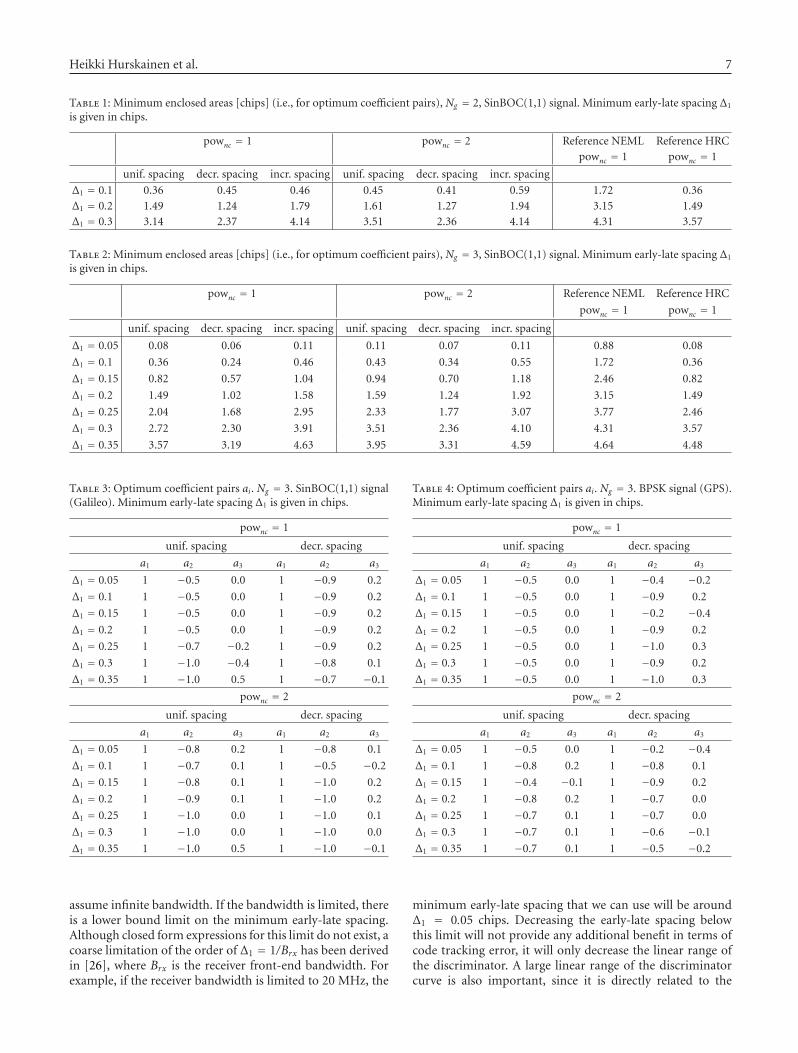
Heikki Hurskainen et al. 7
Table 1: Minimum enclosed areas [chips] (i.e., for optimum coefficient pairs), Ng = 2, SinBOC(1,1) signal. Minimum early-late spacing Δ1
is given in chips.
pownc = 1 pownc = 2 Reference NEML Reference HRCpownc = 1 pownc = 1
unif. spacing decr. spacing incr. spacing unif. spacing decr. spacing incr. spacing
Δ1 = 0.1 0.36 0.45 0.46 0.45 0.41 0.59 1.72 0.36Δ1 = 0.2 1.49 1.24 1.79 1.61 1.27 1.94 3.15 1.49Δ1 = 0.3 3.14 2.37 4.14 3.51 2.36 4.14 4.31 3.57
Table 2: Minimum enclosed areas [chips] (i.e., for optimum coefficient pairs), Ng = 3, SinBOC(1,1) signal. Minimum early-late spacing Δ1
is given in chips.
pownc = 1 pownc = 2 Reference NEML Reference HRC
pownc = 1 pownc = 1
unif. spacing decr. spacing incr. spacing unif. spacing decr. spacing incr. spacing
Δ1 = 0.05 0.08 0.06 0.11 0.11 0.07 0.11 0.88 0.08
Δ1 = 0.1 0.36 0.24 0.46 0.43 0.34 0.55 1.72 0.36
Δ1 = 0.15 0.82 0.57 1.04 0.94 0.70 1.18 2.46 0.82
Δ1 = 0.2 1.49 1.02 1.58 1.59 1.24 1.92 3.15 1.49
Δ1 = 0.25 2.04 1.68 2.95 2.33 1.77 3.07 3.77 2.46
Δ1 = 0.3 2.72 2.30 3.91 3.51 2.36 4.10 4.31 3.57
Δ1 = 0.35 3.57 3.19 4.63 3.95 3.31 4.59 4.64 4.48
Table 3: Optimum coefficient pairs ai. Ng = 3. SinBOC(1,1) signal(Galileo). Minimum early-late spacing Δ1 is given in chips.
pownc = 1
unif. spacing decr. spacing
a1 a2 a3 a1 a2 a3
Δ1 = 0.05 1 −0.5 0.0 1 −0.9 0.2
Δ1 = 0.1 1 −0.5 0.0 1 −0.9 0.2
Δ1 = 0.15 1 −0.5 0.0 1 −0.9 0.2
Δ1 = 0.2 1 −0.5 0.0 1 −0.9 0.2
Δ1 = 0.25 1 −0.7 −0.2 1 −0.9 0.2
Δ1 = 0.3 1 −1.0 −0.4 1 −0.8 0.1
Δ1 = 0.35 1 −1.0 0.5 1 −0.7 −0.1
pownc = 2
unif. spacing decr. spacing
a1 a2 a3 a1 a2 a3
Δ1 = 0.05 1 −0.8 0.2 1 −0.8 0.1
Δ1 = 0.1 1 −0.7 0.1 1 −0.5 −0.2
Δ1 = 0.15 1 −0.8 0.1 1 −1.0 0.2
Δ1 = 0.2 1 −0.9 0.1 1 −1.0 0.2
Δ1 = 0.25 1 −1.0 0.0 1 −1.0 0.1
Δ1 = 0.3 1 −1.0 0.0 1 −1.0 0.0
Δ1 = 0.35 1 −1.0 0.5 1 −1.0 −0.1
assume infinite bandwidth. If the bandwidth is limited, thereis a lower bound limit on the minimum early-late spacing.Although closed form expressions for this limit do not exist, acoarse limitation of the order of Δ1 = 1/Brx has been derivedin [26], where Brx is the receiver front-end bandwidth. Forexample, if the receiver bandwidth is limited to 20 MHz, the
Table 4: Optimum coefficient pairs ai. Ng = 3. BPSK signal (GPS).Minimum early-late spacing Δ1 is given in chips.
pownc = 1
unif. spacing decr. spacing
a1 a2 a3 a1 a2 a3
Δ1 = 0.05 1 −0.5 0.0 1 −0.4 −0.2
Δ1 = 0.1 1 −0.5 0.0 1 −0.9 0.2
Δ1 = 0.15 1 −0.5 0.0 1 −0.2 −0.4
Δ1 = 0.2 1 −0.5 0.0 1 −0.9 0.2
Δ1 = 0.25 1 −0.5 0.0 1 −1.0 0.3
Δ1 = 0.3 1 −0.5 0.0 1 −0.9 0.2
Δ1 = 0.35 1 −0.5 0.0 1 −1.0 0.3
pownc = 2
unif. spacing decr. spacing
a1 a2 a3 a1 a2 a3
Δ1 = 0.05 1 −0.5 0.0 1 −0.2 −0.4
Δ1 = 0.1 1 −0.8 0.2 1 −0.8 0.1
Δ1 = 0.15 1 −0.4 −0.1 1 −0.9 0.2
Δ1 = 0.2 1 −0.8 0.2 1 −0.7 0.0
Δ1 = 0.25 1 −0.7 0.1 1 −0.7 0.0
Δ1 = 0.3 1 −0.7 0.1 1 −0.6 −0.1
Δ1 = 0.35 1 −0.7 0.1 1 −0.5 −0.2
minimum early-late spacing that we can use will be aroundΔ1 = 0.05 chips. Decreasing the early-late spacing belowthis limit will not provide any additional benefit in terms ofcode tracking error, it will only decrease the linear range ofthe discriminator. A large linear range of the discriminatorcurve is also important, since it is directly related to the

8 International Journal of Navigation and Observation
ability of the loop to keep the lock. The linear range isdirectly proportional with half of the early-late spacing Δ1/2,as illustrated in Figure 7 (there, the linear range for Δ1 = 0.1chips goes from −0.05 till 0.05 chips, and the linear rangefor Δ1 = 0.3 chips goes from −0.1 till 0.1 chips, with highlikelihood that the loop will not lose lock as long as theerror is below 0.15 chips in absolute value, due to the piece-wise linear and monotonic shape of the discriminator in theregion −0.15 to 0.15 chips). An approximation of the linearrange of the discriminator is therefore given by Δ1/2. Thus,when choosing Δ1, the designer should take into account themultipath performance, on one hand, and the bandwidthlimitations and linear range constraints, on the other hand.
3.4. MEEs for more than 2 paths
When we want to analyze the MEEs in channels with morethan 2 paths, there are no analytical expressions to computethem, due to the complexity of channel interactions. Thus,we cannot know if the “worst” case errors happen when allthe paths are in phase or when they have alternate phases,and so forth. The solution we propose here in order tocompute MEEs for multiple-paths channels is based onMonte-Carlo simulations: we generate a sufficient numberof random channel realizations Nrandom, and we look atthe highest positive and negative multipath errors over theNrandom points. The goal is to study the MGD performance inmultipath channels with more than 2 channel paths (whichmay occur especially in and urban indoor scenarios). For thispurpose, we consider that the channel impulse response h(t)is given by (same notations from (2) are used here)
h(t) =L∑
l=1
αle− jθl δ
(t − τl
). (13)
We made the following assumptions during the followingsimulations: that the channel has a decaying power delayprofile (PDP), meaning that αl = α1e−μ(τl−τ1), where μis the PDP coefficient (assumed in the simulations to beuniformly distributed in the interval [0.5; 1] when the pathdelays are expressed in samples), that the channel path phasesθl are uniformly distributed in the interval [0; 2π], thatthe number of channel paths L is uniformly distributedbetween 2 and Lmax (with Lmax = 3, 4, . . . ,n), and that thesuccessive path spacing τl − τl−1 is uniformly distributed inthe interval [1/NsNB; xmax], where Ns is the oversamplingfactor or number of samples per BOC interval (a parameterwhich defines the resolution of the delay estimates), andxmax is the maximum value of the successive path spacing(which will define the multipath delay axis in the MEEcurves). It follows that, for each channel realization (meaninga combination of amplitudes α = α1, . . . ,αL, phases θ =θ1, . . . , θL, path spacings, and number of channel paths L),a certain LOS delay is estimated τ1(α, θ,L) from the zerocrossing of the discriminator function (D(τ)|τ1(α,θ,L) = 0),searched in the linear region of D(·). The LOS estimationerror is thus τ1(α, θ,L) − τ1, where τ1 is the true LOS pathdelay. The multipath error envelopes (upper and lower) for a
0 0.5 1 1.5
Multipath delays (chips)
−20
−15
−10
−5
0
5
10
15
20
Cod
etr
acki
ng
erro
r(m
eter
s)
MEEs
NEMLHRC
MGD, uniformMGD, decreasing
Figure 6: Illustration of the averaged MEEs for NEML, HRC,and two MGDs with optimal parameters as given in Table 3 (foruniform and decreasing spacings). pownc = 1, Δ1 = 0.25 chips, andSinBOC(1,1) signals.
−1 −0.5 0 0.5 1
Delay error (chips)
−1
−0.8
−0.6
−0.4
−0.2
0
0.2
0.4
0.6
0.8
1
Dis
crim
inat
orou
tpu
t(n
on-c
oher
ent)
S curve for single path, MGDs
with decreasing spacing, SinBOC(1, 1)
Linear range
Δ1 = 0.1 chipsΔ1 = 0.3 chips
Figure 7: Illustration of the linear range of the discriminator, whenwe increase the minimum early-late spacing. MGDs with Ng = 3,decreasing spacings, pownc = 1, and optimal parameters as given inTable 3.
particular path spacing xmax can be therefore computed as
MEEupper(xmax
) = maxα,θ,L
(τ1(α, θ,L)− τ1
),
MEElower(xmax
) = minα,θ,L
(τ1(α, θ,L)− τ1
).
(14)

Heikki Hurskainen et al. 9
0 0.2 0.4 0.6 0.8 1
Multipath delay spacing xmax (chips)
−50
0
50
100
150
200
250
Cod
etr
acki
ng
erro
r(m
eter
s)
MEEs, Lmax = 6 paths
NEML, pownc = 1, a = [1, 0, 0]NEML, pownc = 2, a = [1, 0, 0]HRC, pownc = 1, a = [1,−0.5, 0]HRC, pownc = 2, a = [1,−0.5, 0]MGD, uniform, pownc = 2, a = [1,−1, 0]MGD, uniform, pownc = 1, a = [1,−0.7, 0.2]MGD, decreasing, pownc = 2, a = [1,−1, 0.1]MGD, decreasing, pownc = 1, a = [1,−0.9, 0.2]
Figure 8: Multipath error envelopes for channels with more than2 paths (Lmax = 6 paths), minimum early-late spacing Δ1 = 0.25chips, SinBOC(1,1) signal.
The results based on the above rule are shown in Figure 8for Lmax = 6 maximum channel paths. Similar results havebeen achieved also for Lmax between 3 and 5 paths, withthe only difference that the MEE levels are increasing whenthe number of path increases (this can be noticed alsoif we compare Figure 8 with Figure 6). Several structureswith optimized parameters as given in Table 3 and differentnonlinearity types were used here. The surprising result isthat the higher the number of channel paths is, the morethe performance of various MGD structures becomes similarfor all the considered algorithms (and they all reach theperformance of the narrow correlator). It follows that themain advantage of the proposed MGD structures comesfrom the fact that they offer patent-free alternatives to thecurrent narrow and double-delta correlators, by preservingthe same performance in realistic multipath channels.
4. SIMULINK/GRANADA-BASED IMPLEMENTATION
4.1. Model description
The Galileo receiver analysis and design application(GRANADA), developed by Deimos Space within GARDAproject, is one of the popular GNSS simulation toolsnowadays. It consists of two parts: Bit-true GNSS SW receiversimulator and GNSS Environment and Navigation simulator.Since the Bit-true GNSS SW receiver simulator is createdbased on the Simulink/Matlab, it is easy to be modified for
new receiver technologies. This simulator is currently usedby several universities and researchers [16, 27–29].
The GRANADA Bit-true GNSS SW receiver simulatoris made up by three parts: the transmitter block, thepropagation channel block, and receiver block, as shownin Figure 9. The transmitter block includes the code gen-eration, BOC modulation, and channel multiplexing. Thepropagation channel model takes into consideration themultipaths, the AWGN noise, and a few other possiblesources of interference, such as the wideband interferencefrom other satellites. The receiver block contains basicallyreceiver front end, acquisition, and code tracking blocks.The general architecture of receiver is shown in Figure 10.After some modification in GRANADA version 2.02, whichis distributed under Galileo supervisory authority (GSA)licenses, it can be used for testing the performance of MGDstructure. The modifications made to GRANADA tool areexplained with details in [29, 30].
4.2. Results in AWGN and multipath static andfading channels
In order to evaluate the performance of the new structures,root mean square error (RMSE) between the estimated delayand the true LOS delay is calculated. In order to test the DLLperformance in the noise presence, we chose three kinds ofchannel profiles: single-path static channel, two-path staticchannel, and four-path fading channel, as shown in Table 5.
Figures 11, 12, and 13 show the RMSE values ofdifferent algorithms in the different channel settings. Sincethe received signal cannot get synchronized in the acquisitionstage of GRANADA when CNR is below 35 dB-Hz, wecalculate the RMSE values from 35 dB-Hz to 50 dB-Hz.Structures with early-late spacing Δ1 = 0.1 chips have beenselected for comparison purpose, but similar results (whichare in accordance with the models given in Section 3) wereobtained for other early-late spacings as well.
Besides the MGD structures described in Section 3, wealso considered here a normalized MGD structure, where thediscriminator function is normalized by the weighted sum ofearly and late correlations, similar with [15, 16]:
Dnorm(τ)
= D(τ)∑Ng
i=1ai(Rc/nc
(τ + Δi/2, fD
)+ Rc/nc
(τ − Δi/2, fD
)) .
(15)
The purpose of including the normalized MGD in the com-parison was to show that the normalized MGD structuresof [15, 16] have worse performance than the un-normalizedstructures proposed by us.
The delay error between the initial code replica in thereceiver and the received signal has not been taken intoaccount. The estimated delay values used for calculatingRMSE are taken after the transient stage in the beginning ofthe tracking stage. From Figures 11 and 12, the simulationresults in the static channel show that as CNR increases, theestimation delay errors converge to the corresponding valuein the MEEs.

10 International Journal of Navigation and Observation
Single (c)
[93330× 1]
Single (c)
[93330× 1]
Bit-true GNSS SW receiver simulator
Galileo transmitterPropagation channel
Galileo receiver
Figure 9: The basic diagram of GRANADA Bit-true software receiver simulator.
Incomingsignal
Half slotaccumulator
∑
A/D∑
Half slotaccumulator
∑
Half slotaccumulator
BOC
BOC
BOC
∑
Chipaccumulator
∑
Chipaccumulator
∑
Chipaccumulator
PN code
PN code
PN code
∑
Dataaccumulator
∑
Dataaccumulator
∑
Dataaccumulator
Data bits
PR and CFmeasurements
Acquisition
Code tracking DLL
Carrier trackingCostas PLL, FLL
PLL/FLL outputshort loop
DLL output
Figure 10: The simplified baseband receiver diagram in GRANADA (NEML).
For scenario 1, the estimated delay errors are causedby the noise only, since there is only LOS signal in thepropagation channel. As the CNR increases, the RMSE valueof each algorithm gets close to 0. When CNR is equal to50 dB-Hz, the RMSE values are below 0.5 meters. Fromthe single path simulation results, we notice that all thesealgorithms have similar performance in the AWGN channel,as desired.
For scenario 2, as the CNR increases, the RMSE value ofeach algorithm converge to different values. This is becausethe RMSE value takes both bias and variance into account.The variance is caused by the noise and decreases when CNRincreases. However, the bias is caused by the multipath inthe channel and is equal to the corresponding point in theMEEs. For instance, as the CNR increases, the RMSE valuesof NEML algorithm converge to 11 meters, which is thesame value in the MEEs according to the channel profile ofscenario 2. The normalized MGD has worse behavior thanan un-normalized MGD with the same parameters.
From Figure 12, it is clear that the HRC algorithm andMGD algorithm with weighting factors a = (1,−0.6, 0)show better performance than NEML algorithm, and MGDalgorithm with a = (1,−0.7, 0.1) (i.e., optimum parameters)shows the best performance among all considered algorithms(which is in accordance with the theoretical derivations inSection 3.2).
In the multipath fading channel, the LOS signal followsRician distribution, and the NLOS signals follow Rayleighdistribution. The mean power and delay of each ray aredescribed in Table 5. Figure 13 shows that the RMSE valueof NEML is much higher than other algorithms, especiallywhen CNR is 35 dB-Hz, it gets till 172 meters (not shown inthe figure in order to get a better scale). An MGD structurewith weighting factor a = (1,−0.7, 0.1) shows again the bestperformance among the algorithms, as expected, accordingto the optimization results given in Section 3. The RMSEperformance of normalized MGD algorithm is quite poor infading channels.

Heikki Hurskainen et al. 11
Table 5: Simulation scenarios for Simulink/GRANADA-based simulations.
Scenario Multipath model Path delay (chip) Relative path gain (dB)
Scenario 1 single-path static channel 0 0
Scenario 2 two-path static channel [0 0.2] [0 −3]
Scenario 3 four-path fading channel [0 0.2 0.4 0.6] [0 −1 −2 −3]
35 40 45 50
CNR (dBHz)
0
0.5
1
1.5
2
2.5
RM
SE(m
)
RMSE in AWGN channel, uniform spacing,Δ1 = 0.1 chips
NEML, a = [1, 0, 0]HRC, a = [1,−0.5, 0]MGD, a = [1,−0.6, 0]
MGD, a = [1,−0.7, 0.1]Normalized MGD, a = [1,−0.7, 0.1]
Figure 11: The RMSE simulation results in single-path staticchannel, Δ1 = 0.1 chips, pownc = 2.
35 40 45 50
CNR (dBHz)
0
2
4
6
8
10
12
RM
SE(m
)
RMSE in 2-path static channel, uniform spacing,Δ1 = 0.1 chips
NEML, a = [1, 0, 0]HRC, a = [1,−0.5, 0]MGD, a = [1,−0.6, 0]
MGD, a = [1,−0.7, 0.1]Normalized MGD, a = [1,−0.7, 0.1]
Figure 12: The RMSE simulation results in two-path static channel,Δ1 = 0.1 chips, pownc = 2.
35 40 45 50
CNR (dBHz)
0
10
20
30
40
50
RM
SE(m
)
RMSE in 4-path fading channel, uniform spacing,Δ1 = 0.1 chips
NEML, a = [1, 0, 0]HRC, a = [1,−0.5, 0]MGD, a = [1,−0.6, 0]
MGD, a = [1,−0.7, 0.1]Normalized MGD, a = [1,−0.7, 0.1]
Figure 13: RMSE simulation results in 4-path fading channel, Δ1 =0.1 chips, pownc = 2.
5. ALGORITHM TESTING/PROTOTYPING
From the MGD structure optimization results (Tables 2and 3), we chose the MGD algorithm with Ng = 3 to beinvestigated further in prototype stage. Both uniform anddecreasing spacings with the Δ1 = 0.1 and Δ1 = 0.25 chipswere chosen to be studied.
The purpose here is to show that the chosen trackingalgorithms are feasible to be implemented on actual devices.One of the targets of this study was to see if the behavior ofthe proposed algorithms does change due to the restrictionsgiven by the hardware implementation. These restrictionsinclude finite computation accuracy, and the effect of quan-tization due to the bit-width of the signals and the limitationcaused by the operation frequency of the synchronous digitalsystem.
We also focus on the design complexity issue, whichcharacterizes the algorithm development especially in thelow cost receivers. Since the trend in price of the satellitenavigation receivers is currently descending [31], the man-ufacturers of these low cost, mass market, receivers willmost likely reject the algorithms with high implementationcomplexity and cost.
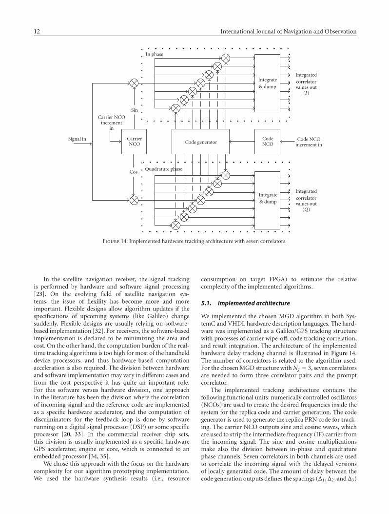
12 International Journal of Navigation and Observation
Integrate& dump
Integrate& dump
CodeNCOCode generator
CarrierNCO
Carrier NCOincrement
in
Integratedcorrelatorvalues out
(I)
Code NCOincrement in
Integratedcorrelatorvalues out
(Q)
Signal in
In phase
Quadrature phaseCos
Sin
Figure 14: Implemented hardware tracking architecture with seven correlators.
In the satellite navigation receiver, the signal trackingis performed by hardware and software signal processing[23]. On the evolving field of satellite navigation sys-tems, the issue of flexility has become more and moreimportant. Flexible designs allow algorithm updates if thespecifications of upcoming systems (like Galileo) changesuddenly. Flexible designs are usually relying on software-based implementation [32]. For receivers, the software-basedimplementation is declared to be minimizing the area andcost. On the other hand, the computation burden of the real-time tracking algorithms is too high for most of the handhelddevice processors, and thus hardware-based computationacceleration is also required. The division between hardwareand software implementation may vary in different cases andfrom the cost perspective it has quite an important role.For this software versus hardware division, one approachin the literature has been the division where the correlationof incoming signal and the reference code are implementedas a specific hardware accelerator, and the computation ofdiscriminators for the feedback loop is done by softwarerunning on a digital signal processor (DSP) or some specificprocessor [20, 33]. In the commercial receiver chip sets,this division is usually implemented as a specific hardwareGPS accelerator, engine or core, which is connected to anembedded processor [34, 35].
We chose this approach with the focus on the hardwarecomplexity for our algorithm prototyping implementation.We used the hardware synthesis results (i.e., resource
consumption on target FPGA) to estimate the relativecomplexity of the implemented algorithms.
5.1. Implemented architecture
We implemented the chosen MGD algorithm in both Sys-temC and VHDL hardware description languages. The hard-ware was implemented as a Galileo/GPS tracking structurewith processes of carrier wipe-off, code tracking correlation,and result integration. The architecture of the implementedhardware delay tracking channel is illustrated in Figure 14.The number of correlators is related to the algorithm used.For the chosen MGD structure withNg = 3, seven correlatorsare needed to form three correlator pairs and the promptcorrelator.
The implemented tracking architecture contains thefollowing functional units: numerically controlled oscillators(NCOs) are used to create the desired frequencies inside thesystem for the replica code and carrier generation. The codegenerator is used to generate the replica PRN code for track-ing. The carrier NCO outputs sine and cosine waves, whichare used to strip the intermediate frequency (IF) carrier fromthe incoming signal. The sine and cosine multiplicationsmake also the division between in-phase and quadraturephase channels. Seven correlators in both channels are usedto correlate the incoming signal with the delayed versionsof locally generated code. The amount of delay between thecode generation outputs defines the spacings (Δ1,Δ2, andΔ3)

Heikki Hurskainen et al. 13
Ref codeVVE VE E P L VL
VVLZ−1 Z−1 Z−1 Z−1 Z−1 Z−1
Δ3
Δ2
Δ1
(a) Delay registers with uniform spacing
Ref codeVVE VE E P L VL
VVLZ−1 Z−2 Z−4 Z−4 Z−2 Z−1
(b) Delay registers with decreasing spacing
Figure 15: Implemented delay registers: (a) uniform delay spacing, (b) decreasing delay spacing. Ref code is reference code chip valuefrom code generator, VVE, VE, E are early, P is prompt, and L, VL, VVL late outputs of the delay register. The relative correlator spacings(Δ1, Δ2, Δ3) are illustrated on top. Z−1 is the smallest uniform delay.
between the correlators. Discriminator function is computedfrom the accumulated (integrated) correlator outputs.
Since we decided to implement both uniform anddecreasing spacing algorithms, two versions of the delay linein the code generator output was constructed. The maindifference between these delay lines is illustrated in Figure 15.The uniform delay spacing is created simply by feeding thereference code chip value from the code generator through adelay shift register, where all delays are equal (e.g., for Δ1 =0.25 chips, we have: Z−1 = 0.125 chips). The decreasing delayspacing implementation needs additional registers betweenthe very-very-early (VVE) and very-very-late (VVL) outputsto align the delays correctly (e.g., for Δ1 = 0.25 chips, wehave: Z−1 = 0.03125 chips, Z−2 = 2Z−1 = 0.0625 chips,and Z−4 = 4Z−1 = 0.125 chips). One may notice that thedecreasing delay spaced register implementation needs muchsmaller uniform delay Z−1. The relationship of smallestuniform delay Z−1 in cases of uniform and decreasing delayspacings is
Z−1uniform= 2Ng−1Z−1
decreasing. (16)
5.2. SystemC verification of the architecture
We started the prototyping task by creating a high-levelSystemC model of the hardware tracking channel. SystemCis a C++ library extension which can be used, for example,to cycle accurate hardware architecture modeling [36]. Thesimilarity of the syntax of the hardware description lan-guage with C++ allowed fast prototype generation. Anotherbenefit of using SystemC is that it contains the simulatoritself, thus a stand-alone executable can be created for thesimulations. The developed model was based on the onepublished previously in [37]. In [37], the SystemC hardwaredescription language was used to model an inter-operativeGPS/Galileo code correlator channel. For the MGD trackingalgorithm testing, a carrier wipe-off process was includedto this newer version of model. We developed a Matlabcode to represent the software part of the proposed MGD
tracking algorithms. Matlab was also used for generationof the input signals for the test simulations. The divisionof resources between SystemC model and Matlab softwareenvironment is illustrated in Figure 16. The implementedSystemC model contains the same functional blocks as areillustrated in Figure 14 and, together with the surroundingMatlab environment, principally the same functionality as inFigure 3.
We used this SystemC model to see how the MEEcurves of the proposed MGD algorithms behave whenthe hardware model is used. HRC and NEML algorithmswere implemented for reference purposes. At first stage ofMEE testing, we noticed that the envelopes (pownc = 1)generated with the SystemC model did have a constantnegative offset. This can be seen clearly in Figure 17, wherethe blue-squared curve illustrating the SystemC hardware-based MEE of NEML (Δ1 = 0.1 chips) has a negative offsetwhen comparing to the black-star, plain Matlab based, andreference curve. On the other hand, the hardware model’sMEE shares the same shape with the ideal reference one.
The reason for this behavior was found to be theimperfect frequency generation inside the hardware trackingchannel. When both code generating and sampling fre-quency are generated with the NCO, there is a possibility toa sample slip if the NCO’s frequency resolution is too low.With no noise condition (as MEEs are generated), this hasan effect on the shape of ideal autocorrelation function curve,making it not to have identical sides. We improved the outputaccuracy of NCOs by increasing the accumulation registersize from 24 to 32 bits. This removed the offset from thediscriminator output as can be seen from Figure 18, wherered-diamond curve presents the MEE result with the newNCO size of 32 bits and blue-squared with NCO size of 24bits.
After the issue of the NCO size was dealt with, wemade a conclusion that the proposed MGD algorithms areimplementable, and the implemented hardware architectureis solid for this purpose. An example curve for the uniformlyspaced (Δ1 = 0.1, Δ2 = 0.2, Δ3 = 0.3 chips) MGD

14 International Journal of Navigation and Observation
Matlab m-function
Signaldriver.cpp
Carrierwipeoff.
cpp
Codewipeoff.
cpp
Integrat eet Dump.
cpp
Input file
Pulse.cpp
Output file
Control file
Codegenerator.
cpp
Controldriver.cpp
NCO.cpp
SystemC executable
Figure 16: Block diagram of the implemented high-level SystemC hardware model inside the Matlab software.
0 0.5 1 1.5
Multipath delay (chips)
−15
−10
−5
0
5
10
15
Err
or(m
)
MEE of NEML
Reference 0Reference −180
SystemC 0SystemC −180
Figure 17: Difference between the hardware model and Matlab-based MEE curves of NEML discriminator (Δ1 = 0.1). The blackline presents the behavior of reference Matlab simulation, and theblue curve illustrates the behavior of the SystemC model.
structure (Ng = 3, pownc = 1) is illustrated in Figure 19. Thisfigure shows how the shape of the hardware-based multipathenvelope is similar to the one generated purely in Matlabin Figure 5. Figures 19 and 5 also show the difference inenvelope area when alternating between pownc = 1 andpownc = 2.
0 0.5 1 1.5
Multipath delay (chips)
−10
−8
−6
−4
−2
0
2
4
6
8
Err
or(m
)
MEE of NEML-effect of NCO register size
SystemC 24 register 0SystemC 24 register −180
SystemC 32 register 0SystemC 32 register −180
Figure 18: Effect of the NCO register length to the MEE curvesof NEML discriminator (Δ1 = 0.1 chips) created by the SystemCmodel. The blue-squared curve presents the case when NCOregister size was 24 bits; the red-diamond line is for the case of 32bits.
5.3. VHDL implementation and synthesis
After the architecture of the hardware tracking channel andits functionality with the proposed MGD structure wereverified with the SystemC hardware model, we build a VHDLmodel of the tracking channel. VHSIC hardware description

Heikki Hurskainen et al. 15
0 0.5 1 1.5
Multipath delay (chips)
−5
−4
−3
−2
−1
0
1
2
3
4
Err
or(m
)
SystemC: MEE of MGD (Ng = 3, pownc = 1,Δ = 0.1)
Upper envelopeLower envelope
Figure 19: Example of the SystemC hardware-based MEE of theMGD (Ng = 3, pownc = 1, Δ1 = 0.1 chips, uniform spacing) withSinBOC(1,1) signal.
language (VHDL) is a language designed and optimized fordescribing the behavior of the digital systems, and it is oneof the standard languages among the electronic engineers[16]. Since the VHDL needs a simulator software forsimulation, we used ModelSim software and tool commandlanguage (TCL) scripts to run the simulations for MEEgeneration. The VHDL hardware-based MEE curve of theproposed MGD with both uniform (a = [1,−0.7,−0.2])and decreasing (a = [1,−0.9, 0.2]) spacing implementationsare illustrated in Figure 20. The blue-squared curve presentsthe uniform spaced MGD and the red-circled the decreasingspaced MGD, for both curves the common parameters wereNg = 3, pownc = 1, and Δ1 = 0.25 chips. From the figure, wecan see that the MEE curves of the hardware implementedMGDs are active in the limits set by the theoretical ones,illustrated in Figure 6.
We used the synthesis results of the VHDL model toevaluate the implementation complexity of the proposedalgorithms. The synthesis was done by using the Xilinx ISEsoftware. We varied the number of correlators, since it is thecharacterizing quantity when choosing the MGD algorithmto be implemented (Ng). Our target device was the XilinxVirtex II PRO field programmable gate array (FPGA). FPGAsare reprogrammable digital devices which can be used intasks requiring a high processing speed, like tracking process[32].
The synthesis results are subjected to the target platformand, therefore, they can not be generalized. Because of this,we focused on the comparison between the complexity ofuniform and decreasing delay spaced implementations, witha varying number of correlators. We synthesized only thedelay register part of the hardware architecture since it is theonly part that differs. The results are illustrated in Figure 21and in Table 6. These results indicate that the hardware
0 0.5 1 1.5
Multipath delay (chips)
−20
−15
−10
−5
0
5
10
15
20
Err
or(m
)
VHDL: MEE curves of MGD (Ng = 3, pownc = 1,Δ = 0.25)
Uniform spacingDecreasing spacing
Figure 20: Example of VHDL hardware-based MEEs. MGD withuniform spacing (a = [1,−0.7,−0.2]) is illustrated in blue-squared curve and MGD with decreasing spacing is illustrated (a =[1,−0.9, 0.2]) in red-circled. (Ng = 3, pownc = 1, Δ1 = 0.25).
2 3 4 5
Ng
100
200
300
400
500
600
700
Equ
ival
ent
logi
cga
teco
un
t
Implementation complexity trends
Uniform spacingDecreasing spacing
Figure 21: Synthesis of the architecture to the target device: effectof the number of correlators.
complexity, measured as usage of target FPGA resources(equivalent logic gate count, logic slices, flip flops, andlookup tables), increases linearly with respect to amount ofcorrelators (Ng) in uniform delay spaced implementations.In cases of decreasing delay spaced implementations,. thecomplexity increase is much faster. One must note that theleft out part of the system adds a constant positive offset tothe synthesis results.
Another difference between the implementations of uni-form and decreasing delay spacings is in the increase of the
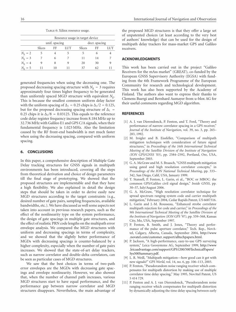
16 International Journal of Navigation and Observation
Table 6: Xilinx resource usage.
Resource usage in target device
unif. spacing decr. spacing
Slices FF LUT Slices FF LUT
Ng = 2 5 4 5 5 6 4
Ng = 3 7 6 7 11 14 7
Ng = 4 9 8 9 20 30 9
Ng = 5 11 10 11 37 62 11
generated frequencies when using the decreasing one. Theproposed decreasing spacing structure with Ng = 3 requiresapproximately four times higher frequency to be generatedthan uniformly spaced MGD structure with equivalent Ng .This is because the smallest common uniform delay factorwith the uniform spacing of Δ1 = 0.25 chips is Δ1/2 = 0.125,but for the proposed decreasing spacing structure of Δ1 =0.25 chips it is Δ1/8 = 0.03125. This equals to the referencecode delay register frequency increase from 8.184 MHz up to32.736 MHz with Galileo E1 and GPS C/A signals, when theirfundamental frequency is 1.023 MHz. Also the limitationcaused by the RF front-end bandwidth is met much fasterwhen using the decreasing spacing, compared with uniformspacing.
6. CONCLUSIONS
In this paper, a comprehensive description of Multiple GateDelay tracking structures for GNSS signals in multipathenvironments has been introduced, covering all the stepsfrom theoretical derivation and choice of design parameterstill the final stage of prototyping. We showed that theproposed structures are implementable and that they havea high flexibility. We also explained in detail the designsteps that should be taken in order to derive easily newMGD structures according to the target constraints (e.g.,desired number of gate pairs, sampling frequencies, availablebandwidths, etc.). We have discussed as well some aspects nottaken into account in previous research papers, such as theeffect of the nonlinearity type on the system performance,the design of gate spacings in multiple gate structures, andthe effect of realistic PRN code lengths on the multipath errorenvelope analysis. We compared the MGD structures withuniform and decreasing spacings in terms of complexity,and we showed that the slightly better performance ofMGDs with decreasing spacings is counter-balanced by ahigher complexity, especially when the number of gate pairsincreases. We showed that the state-of-art delay trackers,such as narrow correlator and double-delta correlators, canbe seen as particular cases of MGD structures.
We saw that the best choices in terms of two-patherror envelopes are the MGDs with decreasing gate spac-ings and envelope nonlinearity. However, we also showedthat, when the number of channel path increases, variousMGD structures start to have equal performance, and theperformance gap between narrow correlator and MGDstructures disappears. Nevertheless, the main advantage of
the proposed MGD structures is that they offer a large setof unpatented choices (at least according to the very bestof authors’ knowledge) that can be used for the design ofmultipath delay trackers for mass-market GPS and Galileoreceivers.
ACKNOWLEDGMENTS
This work has been carried out in the project “GalileoReceivers for the mAss market” (GREAT), co-funded by theEuropean GNSS Supervisory Authority (EGSA) with fund-ing from the 6th Framework Programme of the EuropeanCommunity for research and technological development.This work has also been supported by the Academy ofFinland. The authors also want to express their thanks toClemens Buergi and Bernhard Aumayer from u-blox AG fortheir useful comments regarding MGD algorithm.
REFERENCES
[1] A. J. van Dierendonck, P. Fenton, and T. Ford, “Theory andperformance of narrow correlator spacing in a GPS receiver,”Journal of the Institute of Navigation, vol. 39, no. 3, pp. 265–283, 1992.
[2] M. Irsigler and B. Eissfeller, “Comparison of multipathmitigation techniques with consideration of future signalstructures,” in Proceedings of the 16th International TechnicalMeeting of the Satellite Division of the Institute of Navigation(ION GPS/GNSS ’03), pp. 2584–2592, Portland, Ore, USA,September 2003.
[3] G. A. McGraw and M. S. Braasch, “GNSS multipath mitigationusing gated and high resolution correlator concepts,” inProceedings of the ION National Technical Meeting, pp. 333–342, San Diego, Calif, USA, January 1999.
[4] T. Stansell, P. Fenton, L. Garin, et al., “BOC or MBOC: thecommon GPS/Galileo civil signal design,” Inside GNSS, pp.30–37, July/August 2006.
[5] G. A. McGraw, “High resolution correlator technique forspread spectrum ranging system code and carrier multipathmitigation,” February 2004, Cedar Rapids Patent, US 6687316.
[6] L. Garin and J.-M. Rousseau, “Enhanced strobe correlatormultipath rejection for code and carrier,” in Proceedings of the9th International Technical Meeting of the Satellite Division ofthe Institute of Navigation (ION GPS ’97), pp. 559–568, KansasCity, Mo, USA, September 1997.
[7] P. Fenton, B. Smith, and J. Jones, “Theory and perfor-mance of the pulse aperture correlator,” Tech. Rep., NovA-tel, Calgary, Alberta, Canada, September 2004, http://www.novatel.com/customer support/alltechpapers.html.
[8] P. Jackson, “A high-performance, easy-to-use GPS surveyingsystem,” Leica Geosystems AG, September 1999, http://www.leicaadvantage.com/support/GPS1200/500TechnicalPapers/Sys500Summary.pdf.
[9] L. R. Weill, “Multipath mitigation—how good can it get withnew signals?” GPS World, vol. 14, no. 6, pp. 106–113, 2003.
[10] P. Fenton, “Pseudorandom noise ranging receiver which com-pensates for multipath distortion by making use of multiplecorrelator time delay spacing,” May 1995, NovAtel Patent, US5 414 729.
[11] P. Fenton and A. J. van Dierendonck, “Pseudorandom noiseranging receiver which compensates for multipath distortionby dynamically adjusting the time delay spacing between early

Heikki Hurskainen et al. 17
and late correlators,” February 1996, NovAtel Patent, US 5 495499.
[12] E. S. Lohan, Multipath delay estimators for fading channels withapplications in CDMA receivers and mobile positioning, Ph.D.thesis, Tampere University of Technology, Tampere, Finland,October 2003.
[13] E. S. Lohan, R. Hamila, A. Lakhzouri, and M. Renfors,“Highly efficient techniques for mitigating the effects ofmultipath propagation in DS-CDMA delay estimation,” IEEETransactions on Wireless Communications, vol. 4, no. 1, pp.149–162, 2005.
[14] E. S. Lohan, A. Lakhzouri, and M. Renfors, “Feedforward delayestimators in adverse multipath propagation for Galileo andmodernized GPS signals,” EURASIP Journal on Applied SignalProcessing, vol. 2006, Article ID 50971, 19 pages, 2006.
[15] P. A. Bello and R. L. Fante, “Code tracking performancefor novel unambiguous m-code time discriminators,” MITRETechnical Report, MITRE, Bedford, Mass, USA, 2006.
[16] D. de Castro, J. Diez, A. Fernandez, and J.-M. Sleewaegen, “Anew unambiguous low-complexity BOC tracking technique,”in Proceedings of the 19th International Technical Meeting of theSatellite Division of the Institute of Navigation (ION GNSS ’06),pp. 1830–1835, Fort Worth, Tex, USA, September 2006.
[17] L. R. Weill, “Achieving theoretical bounds for receiver-basedmultipath mitigation using Galileo OS signals,” in Proceedingsof the 19th International Technical Meeting of the SatelliteDivision of the Institute of Navigation (ION GNSS ’06), pp.1035–1047, Fort Worth, Tex, USA, September 2006.
[18] V. A. Veitsel, A. Zhdanov, and M. I. Zhodzishsky, “Themitigation of multipath errors by strobe correlators inGPS/GLONASS receivers,” GPS Solutions, vol. 2, no. 2, pp. 38–45, 1998.
[19] G. A. McGraw, “Practical GPS carrier phase multipathmitigation using high resolution correlator techniques,” inProceedings of the IAIN World Congress and the 56th AnnualMeeting of the Institute of Navigation, pp. 373–381, San Diego,Calif, USA, June 2000.
[20] E. D. Kaplan and C. J. Hegarty, Eds., Understanding GPS,Principles and Applications, Artech House, Boston, Mass, USA,2nd edition, 2006.
[21] Galileo Joint Undertaking, “Galileo open service, signal inspace interface control document (OS SIS ICD),” May 2006,http://www.galileoju.com/.
[22] E. S. Lohan, A. Lakhzouri, and M. Renfors, “Binary-offset-carrier modulation techniques with applications in satellitenavigation systems,” Wireless Communications and MobileComputing, vol. 7, no. 6, pp. 767–779, 2007.
[23] M. S. Braasch and A. J. van Dierendonck, “GPS receiverarchitectures and measurements,” Proceedings of the IEEE, vol.87, no. 1, pp. 48–64, 1999.
[24] D. Skournetou and E. S. Lohan, “Non-coherent multiplecorrelator delay structures and their tracking performancefor Galileo signals,” in Proceedings of the European NavigationConference (ENC-GNSS ’07), Geneva, Switzerland, May-June2007.
[25] T. Pany, M. Irsigler, and B. Eissfeller, “S-curve shaping: anew method for optimum discriminator based code multipathmitigation,” in Proceedings of the 18th International TechnicalMeeting of the Satellite Division of the Institute of Navigation(ION GNSS ’05), Long Beach, Calif, USA, September 2005.
[26] R. van Nee, Multipath and multi-transmitter interference inspread-spectrum communication and navigation systems, Ph.D.thesis, Delft University of Technology, Delft, The Netherlands,1995.
[27] J. Diez, A. Fernandez, J. S. Silva, L. Marradi, and V. Gabaglio,“Characterization of the pseudorange error due to codedoppler shift in Galileo E5 and L1 receivers using theGRANADA bit-true simulator,” in Proceedings of the 18thInternational Technical Meeting of the Satellite Division of theInstitute of Navigation (ION GNSS ’05), Long Beach, Calif,USA, September 2005.
[28] J. Won, T. Pany, and G. Hein, “GNSS software defined radio:real receiver or just a tool for experts,” Inside GNSS, vol. 1, no.5, pp. 48–56, July/August 2006.
[29] X. Hu and E. S. Lohan, “GRANADA validation of optimizedmultiple gate delay structures for Galileo SinBOC(1,1) signaltracking,” in Proceedings of the 7th International Conference onITS Telecommunications (ITST ’07), pp. 1–5, Sophia Antipolis,France, June 2007.
[30] H. Hurskainen, X. Hu, S. Ancha, G. Bell, J. Raasakka, andJ. Nurmi, “Enhancing usability of the GRANADA bit-truereceiver simulation on Galileo L1,” in Proceedings of the 20thInternational Technical Meeting of the Satellite Division of TheInstitute of Navigation (ION GNSS ’07), Fort Worth, Tex, USA,September 2007.
[31] S. Colwell, “The price is right! GPS prices drop for consumers,”GPS World, vol. 18, no. 5, pp. 31–32, 2007.
[32] F. Dovis, A. Gramazio, and P. Mulassano, “SDR technologyapplied to Galileo receivers,” in Proceedings of the 15thInternational Technical Meeting of the Satellite Division of theInstitute of Navigation (ION GPS ’02), Portland, Ore, USA,September 2002.
[33] D. Benson, “The design and implementation of a GPS receiverchannel,” Xilinx: DSP Magazine, pp. 50–53, October 2005.
[34] u Blox, “UBX-G5010 product summary sheet,” April 2007,http://www.u-blox.com/products/Product Summaries/UBX-G5010 Prod Summary(GPS.G5-X-06042).pdf.
[35] Sirf, “SiRFstarIII GSC3LP Product Insert,” http://www.sirf.com/products/GSC3LPProductInsert.pdf.
[36] SystemC Version 2.0 User’s Guide.[37] H. Hurskainen and J. Nurmi, “SystemC model of an interop-
erative GPS/Galileo code correlator channel,” in Proceedingsof the IEEE Workshop on Signal Processing Systems Designand Implementation (SIPS ’06), pp. 327–332, Banff, Alberta,Canada, October 2006.

Publication 4
c©2008 IEEE. Reprinted, with permission, from Proceedings of 4th Advan-ced Satellite Mobile Systems (ASMS) conference 2008, “GNSS Receiver Re-ference Design”, Heikki Hurskainen, Tommi Paakki, Zhongqi Liu, Jussi Raa-sakka, and Jari Nurmi.
This material is posted here with permission of the IEEE. Such permission of theIEEE does not in any way imply IEEE endorsement of any of the Tampere Universityof Technology’s products or services. Internal or personal use of this material ispermitted. However, permission to reprint/republish this material for advertising orpromotional purposes or for creating new collective works for resale or redistributionmust be obtained from the IEEE by writing to [email protected].
By choosing to view this material, you agree to all provisions of the copyright lawsprotecting it.
Heikki Hurskainen, Tommi Paakki, Zhongqi Liu, Jussi Raasakka, and Jari Nurmi Department of Computer Systems
Tampere University of Technology
Tampere, Finland
Abstract - Satellite based navigation is a rapidly growing
application of satellite systems. The research of the topic is
lacking “open source” hardware receivers. Our group’s
purpose is to provide one. In this paper we outline the
background to the topic, motivate the need for hardware
receiver research and present the functional blocks for a
generic GNSS receiver. Our implementations, with their
current status, are presented and the initial block-by-block
functionality is presented along the signal chain from antenna
to the actual navigation solution. Our future work will be the
connection of the currently discrete pieces to a solid
framework – a real-time GNSS receiver.
I. INTRODUCTION
NE of the fastest growing applications of satellite
systems is the satellite based navigation. Out of the
current Global Navigation Satellite Systems (GNSS)
the American NAVSTAR Global Positioning System, a.k.a.
GPS, is the only one with fully operational status and 99%
service coverage over the world [1]. The other system
partially existing is Russian GLONASS, which is currently
on the edge of total system renewal.
Europe has also started operation in the GNSS field. The
first Galileo test satellite, GIOVE-A, was launched on 28th
of December in 2005 [2]. The second test satellite, GIOVE-
B was launched on 27th of April 2008 and GIOVE-A2 is
planned to be launched in 2009 [2], [3].
The fourth player in the GNSS field is China. The
Chinese system called Beidou/Compass is already
transmitting preliminary signals [4].
With so many systems emerging and the GPS
modernization program existing [1] it is clear that there is
much interest in the satellite navigation now and in the
future.
A. Motivation
Since the systems under acronym GNSS are being
developed, the research of related topics, especially
receivers, are also of growing interest.
Research covering GNSS receivers is done in many
abstraction levels, starting from high level algorithm
development to actual building of working prototypes of
receivers. All of these abstraction levels need to be
researched to gain best possible knowledge of the issue.
In the prototyping end of the research there are not many
open source satellite navigation receivers available. The few
existing ones [5], [6] are mostly relying on open source
software, and third party hardware. Or the open source is
limited to architecture level [7]. Yet there are researchers
who are also keen to know what happens inside of the actual
hardware.
From this starting point we started to work up over an
idea of making an open source GNSS receiver reference
design.
B. Selection of the Proper Subset of GNSS Signals
In practice it is hard to build a receiver that works with all
GNSS signals. To select a feasible subset of GNSS signals
the designer must take into account several issues, e.g., the
frequencies and signal availability without cost.
The illustration of the signal spectra of these systems is
shown in Figure 1. As one can see from the figure, some
frequency bands are common between several systems.
Between GPS and Galileo two bands are shared; E5a – L5,
centered at 1176.45 MHz and L1, centered at 1575.42 MHz.
Especially interesting band is the L1 band, since it is
currently the only one actually having a real navigation
signal, GPS C/A, available for civilian users. New L1 band
signals have been introduced, Galileo L1 Open Service
Signal, also free to use for civilians and GPS L1C, an
advanced GPS signal. [10]
The European and US satellite navigation authorities have
closely worked together on interoperatibility issues between
the Galileo L1 OS signals and future advanced GPS L1
signals. This work has yielded a new common modulation
scheme called Binary Offset Carrier modulation [8], [16].
Because of the existing signal (GPS C/A) and future
Galileo OS signal we decided to go with a L1 band receiver.
C. The Concept of GNSS Receiver
The legacy (GPS receiver) for the concept of a GNSS
receiver is well presented in literature [1], [6], [9], from
where our approach is straightforwardly adopted. The high
level block diagram of the GNSS receiver is shown in
Figure 2. Next we give an overview of interfaces and
functions of each block. A more detailed description of the
implementation of those functions is given in later sections.
The receiver interfaces to the satellite system through an
antenna which receives the satellite signals and feeds them
to the Radio Frequency (RF) front end unit of the receiver.
The GPS receiver’s antenna is characterized with Right-
Hand-Circular-Polarization (RHCP), and hemispherical
reception pattern [1].
GNSS Receiver Reference Design
O
978-1-4244-2204-3/08/$25.00 ©2008 IEEE

The radio part in a GNSS receiver contains the same
fundamental parts as any other satellite radio receiver. The
incoming signal is amplified with a low noise amplifier
(LNA), filtered, down-converted to a suitable Intermediate
Frequency (IF) and at last quantized and digitized by an
analog to digital converter. The radio part feeds the digital
signal to the baseband part [6], [10].
The main tasks of the baseband part consisting of parallel
digital receiver channels are to find the satellite signals
buried in noise, and then track them to extract the
demodulated navigation data from the signal. Three-
dimensional navigation needs at least four satellites to solve
four unknowns (x-, y-, z-coordinates, and time), this is the
reason for having at least four parallel channels, each
working on one satellite signal. Typical number of parallel
channels in today’s mass market GPS receivers is 12, when
in practice the number of satellites in view for a certain
location is from 6 to 10 [1].
The search phase is called acquisition. The acquisition is
basically a three dimensional task, the dimensions being
satellite id (each satellite has a unique pseudorandom noise
code), the PRN code delay and the Doppler frequency
caused by the movement of the satellite and receiver.
After successful acquisition the signal can be tracked.
Tracking tries to keep up with the dynamics of the incoming
signal by replicating it as accurately as possible. The error
between the replicated signal and the incoming one is
sensed by feedback loops. Delay Locked Loop (DLL) is
used for PRN code phase tracking and Frequency and/or
Phase Locked Loops (FLL, PLL) are used for tracking the
carrier frequency and phase of the signals respectively.
When signals are locked to the tracking (i.e. the tracking
keeps up with them) the receiver can extract the data
symbols from the data stream. In addition to the navigation
data the signal symbol stream contains preamples (i.e. pre-
defined bit sequences) which are used for synchronizing the
received data (i.e. finding boundaries of the data frames /
sub frames).
Besides demodulation of the navigation data the baseband
tracking must also provide pseudoranges to satellites.
Pseudoranges are computed from time differences between
signal transmission and reception times.
The transmission time of the signal is coded in the
navigation data (called Z count in GPS system), and the
reception time can be calculated by using phase information
provided by the tracking loops and by counting data
symbols and PRN code chips.
The navigation process takes a constant stream of
navigation data as input. This navigation data stream
consists of all separate data streams from the satellites that
are being currently tracked. For each tracked satellite, it is
necessary to decode a certain set of parameters, i.e.,
ephemeris parameters. The ephemeris data describes the
actual satellite orbit, and it also includes parameters which
correct perturbations over time in the satellite orbit.
Before any data is utilized in navigation, it must pass
parity checking. Then as the valid ephemeris data has been
updated for each tracked satellite, it is possible to calculate
the satellite locations in ECEF (Earth Centered Earth Fixed)
coordinates. In the same process, corrections are applied to
the pseudorange values that are provided by the baseband
unit.
In the next phase the user location is estimated. The
estimation is based on typical least-squares (LS) method,
which is an iterative algorithm for estimating user location
and user clock bias. After a number of iterations the solution
will converge to the best estimate of the given satellite
geometry.
The results from the LS method are still noisy, and they
contain a random error from the true user location. This
error is equivalent to the User Equivalent Range Error
(UERE). For providing smoother user location estimates a
Kalman filter can be applied [11]. With a simple filter
model the results can be improved in quality.
Figure 1 Frequency plans for current and planned GPS, Galileo and GLONASS signals. Figure is modified from one presented in [10].
15
45
MH
z
12
78
.85
MH
z
11
76
.45
MH
z
12
27
.6 M
Hz
15
75
.42
MH
z
GLONASS L3 L2 L1
E5a E6
L5 L2
L6 E2 E1Galileo L1
GPS L1
E5b
GPS
Galileo
GLONASS
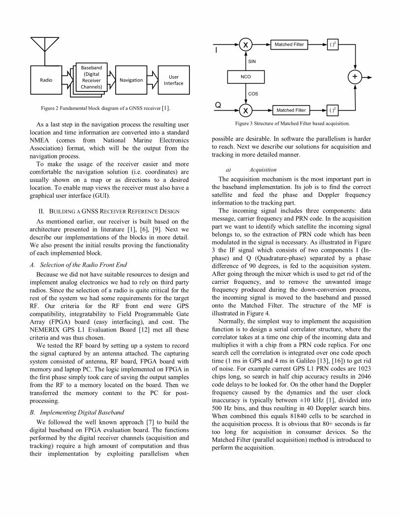
As a last step in the navigation process the resulting user
location and time information are converted into a standard
NMEA (comes from National Marine Electronics
Association) format, which will be the output from the
navigation process.
To make the usage of the receiver easier and more
comfortable the navigation solution (i.e. coordinates) are
usually shown on a map or as directions to a desired
location. To enable map views the receiver must also have a
graphical user interface (GUI).
II. BUILDING A GNSS RECEIVER REFERENCE DESIGN
As mentioned earlier, our receiver is built based on the
architecture presented in literature [1], [6], [9]. Next we
describe our implementations of the blocks in more detail.
We also present the initial results proving the functionality
of each implemented block.
A. Selection of the Radio Front End
Because we did not have suitable resources to design and
implement analog electronics we had to rely on third party
radios. Since the selection of a radio is quite critical for the
rest of the system we had some requirements for the target
RF. Our criteria for the RF front end were GPS
compatibility, integratability to Field Programmable Gate
Array (FPGA) board (easy interfacing), and cost. The
NEMERIX GPS L1 Evaluation Board [12] met all these
criteria and was thus chosen.
We tested the RF board by setting up a system to record
the signal captured by an antenna attached. The capturing
system consisted of antenna, RF board, FPGA board with
memory and laptop PC. The logic implemented on FPGA in
the first phase simply took care of saving the output samples
from the RF to a memory located on the board. Then we
transferred the memory content to the PC for post-
processing.
B. Implementing Digital Baseband
We followed the well known approach [7] to build the
digital baseband on FPGA evaluation board. The functions
performed by the digital receiver channels (acquisition and
tracking) require a high amount of computation and thus
their implementation by exploiting parallelism when
possible are desirable. In software the parallelism is harder
to reach. Next we describe our solutions for acquisition and
tracking in more detailed manner.
a) Acquisition
The acquisition mechanism is the most important part in
the baseband implementation. Its job is to find the correct
satellite and feed the phase and Doppler frequency
information to the tracking part.
The incoming signal includes three components: data
message, carrier frequency and PRN code. In the acquisition
part we want to identify which satellite the incoming signal
belongs to, so the extraction of PRN code which has been
modulated in the signal is necessary. As illustrated in Figure
3 the IF signal which consists of two components I (In-
phase) and Q (Quadrature-phase) separated by a phase
difference of 90 degrees, is fed to the acquisition system.
After going through the mixer which is used to get rid of the
carrier frequency, and to remove the unwanted image
frequency produced during the down-conversion process,
the incoming signal is moved to the baseband and passed
onto the Matched Filter. The structure of the MF is
illustrated in Figure 4.
Normally, the simplest way to implement the acquisition
function is to design a serial correlator structure, where the
correlator takes at a time one chip of the incoming data and
multiplies it with a chip from a PRN code replica. For one
search cell the correlation is integrated over one code epoch
time (1 ms in GPS and 4 ms in Galileo [13], [16]) to get rid
of noise. For example current GPS L1 PRN codes are 1023
chips long, so search in half chip accuracy results in 2046
code delays to be looked for. On the other hand the Doppler
frequency caused by the dynamics and the user clock
inaccuracy is typically between ±10 kHz [1], divided into
500 Hz bins, and thus resulting in 40 Doppler search bins.
When combined this equals 81840 cells to be searched in
the acquisition process. It is obvious that 80+ seconds is far
too long for acquisition in consumer devices. So the
Matched Filter (parallel acquisition) method is introduced to
perform the acquisition.
Radio NavigationUser
Interface
Baseband
(Digital
Receiver
Channels)
Figure 2 Fundamental block diagram of a GNSS receiver [1].
Figure 3 Structure of Matched Filter based acquisition.
NCO
I
Q
SIN
COS
2
( )2
+
x Matched Filter
Matched Filter
( )2
x

Actually, the architecture of Matched Filter is composed
by a number of correlators and an accumulator. First the
PRN code generator produces M PRN chips (1023 in GPS
L1 [13]) and then the replica is held in a register static and
multiplied with M chips of incoming data simultaneously.
The M correlation results will then be summed by the
accumulator and sent to the decision unit. This parallel
acquisition is M times faster than the simple serial
acquisition.
The Matched Filter complexity increases with Galileo
implementation. Since Galileo OS L1 PRN codes are 4092
chips long [16], the needed Matched Filter size is 4 times
bigger. In the decision unit the accumulated value will be
compared with the acquisition threshold value. When the
result from the accumulation is larger than the threshold,
meaning that the satellite has been found, a control signal is
asserted indicating successful acquisition. The delay and
Doppler information of the signal are handed over to the
tracking process.
If the signal is not found the acquisition is continued with
a different Doppler bin. After going through all possible
bins and having no successful acquisition result, or after
successful acquisition, the system will change the satellite
that it is searching for.
b) Tracking
When the control signal sent by the Decision Unit is
detected, the tracking system is activated. The Architecture
of GPS L1 tracking is illustrated in Figure 5. The
Numerically Controlled Oscillator (NCO) is working as a
plant for replica carrier and code generation. The output
speed of the NCOs can be controlled by the input. As
mentioned in the acquisition process, the PRN code
generator stops producing replica after generating all phases
of a PRN code. In the tracking process, the code generator
will start again to produce the PRN at the same phase as the
incoming data. In order not to lose the acquired satellite, the
carrier frequency and code phase should be kept locked.
To improve the accuracy and performance of our tracking
system, we use a quarter chip spacing shifter in the code-
shift register which produces three different phases of the
replica GPS PRN code. In this way, the output frequency of
code shifter is approximately 4 times that of the code
generator.
After code-shifter producing 3 different phases of replica
(early, prompt, late), the replicas are fed to three correlators
and multiplied with the incoming data whose carrier
frequency has already been stripped off. The results from
the correlators are passed onto accumulators and integrated
together over a code epoch time. After correlation and
accumulation, the peak value of the different phases can be
compared. If the incoming data is misaligned with the
replica, the direction and bias will be determined according
to the comparison of these three peak values, and correction
information will be sent back to carrier NCO and code NCO
through Frequency Locked Loop and Delay Locked Loop.
The new carrier frequency and code phase are adjusted to
keep tracking the current incoming signal.
To enhance the structure for Galileo OS L1 and future
GPS L1 signals the number of correlators should be
increased to five, at least [14]. This is because the composite
BOC (CBOC) modulation scheme used in the new signals
will have additional correlation peaks.
C. Role of the Simulation Tools
To proceed with the discrete testing of our blocks we had
to simulate the baseband part, since the interfaces to the
hardware implementation were not ready.
As earlier work we had developed a Matlab/Simulink
based tool for Galileo receiver simulation [15]. We
remapped the functionality of this simulator to pure Matlab
functions and added the GPS compatibility. The result was a
post-processing tool for extraction of navigation data from
raw records of satellite signals. By using this tool we
bridged the RF output to navigation input thus enabling the
development at navigation software side to be independent
from the development on baseband hardware side.
From the recorded data sets we managed to extract
enough data for navigation by using the Matlab simulator
tool.
D. Implementing Navigation Algorithms
The navigation algorithms have been implemented for
Figure 4 Structure of a Matched Filter.
2 M1 3
x x x x
M chip PRN code
M
Data
Figure 5 Architecture of the GPS Early – Late tracking.
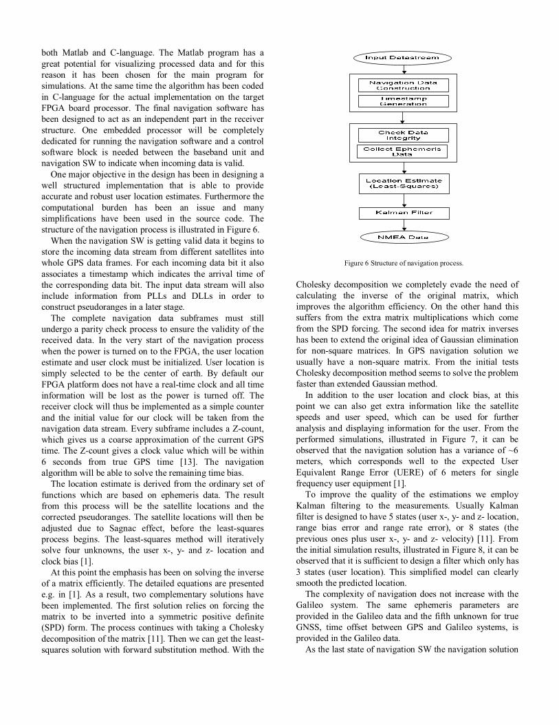
both Matlab and C-language. The Matlab program has a
great potential for visualizing processed data and for this
reason it has been chosen for the main program for
simulations. At the same time the algorithm has been coded
in C-language for the actual implementation on the target
FPGA board processor. The final navigation software has
been designed to act as an independent part in the receiver
structure. One embedded processor will be completely
dedicated for running the navigation software and a control
software block is needed between the baseband unit and
navigation SW to indicate when incoming data is valid.
One major objective in the design has been in designing a
well structured implementation that is able to provide
accurate and robust user location estimates. Furthermore the
computational burden has been an issue and many
simplifications have been used in the source code. The
structure of the navigation process is illustrated in Figure 6.
When the navigation SW is getting valid data it begins to
store the incoming data stream from different satellites into
whole GPS data frames. For each incoming data bit it also
associates a timestamp which indicates the arrival time of
the corresponding data bit. The input data stream will also
include information from PLLs and DLLs in order to
construct pseudoranges in a later stage.
The complete navigation data subframes must still
undergo a parity check process to ensure the validity of the
received data. In the very start of the navigation process
when the power is turned on to the FPGA, the user location
estimate and user clock must be initialized. User location is
simply selected to be the center of earth. By default our
FPGA platform does not have a real-time clock and all time
information will be lost as the power is turned off. The
receiver clock will thus be implemented as a simple counter
and the initial value for our clock will be taken from the
navigation data stream. Every subframe includes a Z-count,
which gives us a coarse approximation of the current GPS
time. The Z-count gives a clock value which will be within
6 seconds from true GPS time [13]. The navigation
algorithm will be able to solve the remaining time bias.
The location estimate is derived from the ordinary set of
functions which are based on ephemeris data. The result
from this process will be the satellite locations and the
corrected pseudoranges. The satellite locations will then be
adjusted due to Sagnac effect, before the least-squares
process begins. The least-squares method will iteratively
solve four unknowns, the user x-, y- and z- location and
clock bias [1].
At this point the emphasis has been on solving the inverse
of a matrix efficiently. The detailed equations are presented
e.g. in [1]. As a result, two complementary solutions have
been implemented. The first solution relies on forcing the
matrix to be inverted into a symmetric positive definite
(SPD) form. The process continues with taking a Cholesky
decomposition of the matrix [11]. Then we can get the least-
squares solution with forward substitution method. With the
Cholesky decomposition we completely evade the need of
calculating the inverse of the original matrix, which
improves the algorithm efficiency. On the other hand this
suffers from the extra matrix multiplications which come
from the SPD forcing. The second idea for matrix inverses
has been to extend the original idea of Gaussian elimination
for non-square matrices. In GPS navigation solution we
usually have a non-square matrix. From the initial tests
Cholesky decomposition method seems to solve the problem
faster than extended Gaussian method.
In addition to the user location and clock bias, at this
point we can also get extra information like the satellite
speeds and user speed, which can be used for further
analysis and displaying information for the user. From the
performed simulations, illustrated in Figure 7, it can be
observed that the navigation solution has a variance of ~6
meters, which corresponds well to the expected User
Equivalent Range Error (UERE) of 6 meters for single
frequency user equipment [1].
To improve the quality of the estimations we employ
Kalman filtering to the measurements. Usually Kalman
filter is designed to have 5 states (user x-, y- and z- location,
range bias error and range rate error), or 8 states (the
previous ones plus user x-, y- and z- velocity) [11]. From
the initial simulation results, illustrated in Figure 8, it can be
observed that it is sufficient to design a filter which only has
3 states (user location). This simplified model can clearly
smooth the predicted location.
The complexity of navigation does not increase with the
Galileo system. The same ephemeris parameters are
provided in the Galileo data and the fifth unknown for true
GNSS, time offset between GPS and Galileo systems, is
provided in the Galileo data.
As the last state of navigation SW the navigation solution
Figure 6 Structure of navigation process.

must be converted into latitude, longitude and altitude
format. After the conversion the results are encoded into
NMEA format. These NMEA messages are then sent to the
GUI of our design via serial port (RS-232). The GUI is
implemented on a laptop PC.
CONCLUSIONS
In this paper we presented the motivation and concept for
a GNSS receiver reference design. We also presented our
implementations, with current status. We presented the
initial block-by-block functionality along the signal chain
from antenna to the filtered navigation solution. We
conclude that we have managed to gather all the pieces and
now we only have to solve the puzzle, which remains as
future work. Achieving real-time operation only requires the
completion of the baseband HW on FPGA. In the future we
will extend the working GPS receiver to work also with
other satellite based navigation systems.
The reference design will then serve as a valuable
platform to experiment novel receiver baseband and
navigation solution algorithms in real time.
ACKNOWLEDGEMENT
This work was partially supported by the Finnish Agency
for Technology and innovation (TEKES) and Finnish
companies within the Future GNSS Applications and
Techniques (FUGAT) project, and Department of Computer
Systems of TUT.
REFERENCES
[1] Kaplan, Elliot D. and Hegarty, Christopher J. “Understanding GSP -
Principles and Applications (Second Edition)”. Norwood. Artech
House, 2006. ISBN-10: 1-58053-894-0.
[2] ESA. GIOVE Webpage. European Space Agency - Navigation.
[Online] 2008. [Cited: June 2, 2008.] http://www.giove.esa.int/.
[3] Rooney, E.; Unwin, M.; Gatti, G.; Falcone, M.; Binda, S.; Malik, M.;
and Hannes, D. “Giove-A In Orbit Testing Results”. In Proceedings
of 2007 ION GNSS, Sep 25-28, 2007. Fort Worth, TX.
[4] Grelier, T.; Ghion, A.; Dantepal, J.; Ries, L.; DeLatour, A.; Issler, J.-
L.; Avila-Rodriguez, J. A.; Wellner, S.; and Hein, G. W. “Compass
Signal Structure and First Measurements”. In Proceedings of 2007
ION GNSS, 25 - 28 Sep, 2007. Fort Worth, TX.
[5] Kelley, Clifford W.;Niles, Frederick and Baker, Douglas.
“Development of the Open Source GPS Software Receiver
Emulator”. In Proceedings of the 2007 ION GNSS, 25-28 Sep, 2007.
Fort Worth, TX:
[6] Borre, K.; Akos, D. M.; Bertelsen, N.; Rinder, P.; and Jensen, S. H.
“A Software-Defined GPS and Galileo Receiver - A Single-
Frequency Approach”. Boston, MA. Birkhauser, 2007.
[7] Engel, Frank, et al. “An Open GNSS Receiver Platform
Architecture”. Journal of Global Positioning Systems, 2004, Vol. 3.
[8] “Interface Specification - Navstar GPS Space segment/User segment
L1C Interfaces”. 04 August 2007. IS-GPS-800.
[9] Braasch, Michael S. and Van Dierendonck, A. J. “GPS Receiver
Architectures and Measurements”. Proceedings of the IEEE, January,
1999, Vol. 87.
[10] Sherman, L.; Chen, A.; Enge, P.; Gao, G.; Akos, D.; Issler, J.-L.;
Ries, L.; Grelier, T.; and Dantepal, J. “Images and Spectral Signatures
of the New GNSS Signals”. InsideGNSS. 2006, May/June.
[11] Brown, Robert G. and Hwang, Patric Y.C. “Introduction to Random
Signals and Applied Kalman Filtering (Third Edition)”. John Wiley &
Sons, 1997. ISBN 0-471-12839-2.
[12] NEMERIX. Datasheet "EB1006A - Evaluation Board for NJ1006A".
October 2005. Rev 1.2..
[13] “NAVSTAR Global Positioning System. Interface Specification, IS-
GPS-200”, Revision D. [Online] 2004.
http://www.navcen.uscg.gov/gps/geninfo/IS-GPS-200D.pdf.
[14] Fine, Paul and Wilson, Warren. “Tracking Algorithm for GPS Offset
Carrier Signals”. In Proceedings of the 1999 ION NTM, Jan 25-27,
1999. San Diego, CA.
[15] Raasakka, Jussi, Hurskainen, Heikki and Nurmi, Jari. ”Galileo
Receiver Design and Analysis Tool Development in Tampere
University of Technology”. In Proceedings of the 2007 ION NTM,
Jan 22-24, 2007. San Diego, CA.
[16] “Galileo Open Service Signal in Space Interface Control Document
(OS SIS ICD)”, Draft 1, Feb 14, 2008
Figure 7 XY-Scatter plot of the navigation results, without filtering.
Crosses represent the discrete results, the point in the middle is the true location and the circle represents the 6 meter variance.
Figure 8 XY-Scatter plot of the navigation results, filtered. Crosses
represent the discrete results, the point in the middle is the true location and the circle represents the 6 meter variance.


Publication 5
c©2008 IEEE. Reprinted, with permission, from Proceedings of InternationalSymposium on System-on-Chip (SOC) 2008, “Specification of GNSS Appli-cation for Multiprocessor Platform”, Heikki Hurskainen, Jussi Raasakka, andJari Nurmi.
This material is posted here with permission of the IEEE. Such permission of theIEEE does not in any way imply IEEE endorsement of any of the Tampere Universityof Technology’s products or services. Internal or personal use of this material ispermitted. However, permission to reprint/republish this material for advertising orpromotional purposes or for creating new collective works for resale or redistributionmust be obtained from the IEEE by writing to [email protected].
By choosing to view this material, you agree to all provisions of the copyright lawsprotecting it.

Specification of GNSS Application for Multiprocessor Platform
Heikki Hurskainen, Jussi Raasakka, and Jari Nurmi Department of Computer Systems
Tampere University of Technology Tampere, Finland
Abstract—In this paper we present a satellite navigation application for a multiprocessor platform. We give a preliminary description to the multiprocessor platform with an introduction to the project where it will be designed and implemented to a fabric die. The platform contains a matrix of processing tiles, connected together via a Network-on-Chip. The satellite navigation application is one of the streaming applications designed to be executed on this platform. Detailed descriptions of the signal processing functions for acquiring and tracking the satellite signals for navigation are given. The estimations of their requirements for computational complexity, measured as multiply-accumulate counts, are also presented in this paper. The results indicate that one processing tile on the platform could barely perform the required signal processing functions and thus more tiles are preferred for a better user experience. This work is carried out in the EU FP7 project called CRISP (Cutting edge Reconfigurable ICs for Stream Processing).
I. INTRODUCTION CRISP (Cutting edge Reconfigurable ICs for Stream
Processing) is a project funded from European Union 7th Framework Program (EU FP7) funds. The CRISP consortium is a good mixture of industrial and academic know-how and competence. The consortium members are: Recore Systems (NL), University of Twente (NL), Atmel (DE), Thales Netherlands (NL), Tampere University of Technology (FI), and NXP (NL).
The main objective of this project is to research the optimal utilization, efficient programming and dependability of a reconfigurable multiprocessor platform for streaming applications. During the project a General Stream Processor (GSP, not to be mixed with the GPS (NAVSTAR Global Positioning System)), a system with multiple cores, will be specified, designed and eventually implemented onto a single fabric die. This multi-core system will consist of a number of Tile Processors (TP), embedded memories and other dedicated blocks, connected via a Network-on-Chip (NoC). The manufactured die will be accompanied by a
General Purpose Processor (GPP) die in a System-in-Package (SiP). The processing tiles are reconfigurable.
The project has four main themes. The Streaming Applications theme is about specification, implementation and integration of the streaming applications to the GSP. The streaming applications selected for the project for proof-of-concept purposes are a beamforming application in electronically steered radar which is out of the scope of this paper, and a Global Navigation Satellite System (GNSS) application.
The streaming applications are developed in parallel with the development of the multiprocessor platform. The goals for developing the streaming applications within the project are to obtain experience in the software development for reconfigurable multi-core systems; improve the design methodology for developing complete streaming applications; obtain realistic design specifications for the GSP; and use realistic streaming applications for evaluating project results. The other themes in the CRISP project are General Stream Processor (GSP), Run-time Mapping and Dependability.
From a GNSS applications point of view the anticipated result of the whole project is to create a software navigation application running on the multi-core platform (General Stream Processor). Expected output of the application is a real-time PVT (Position, Velocity and Time) solution. The application should take full advantage of the available computational resources. To our knowledge the GNSS receiver application running on multiple cores is novel. Examples of implementations of parts of the GNSS/GPS receiver functionality to reconfigurable machines can be found in literature, e.g. in [1] and [2].
This paper is divided to the following sections. The planned CRISP platform is described in Section II, where we discuss the components of the system. Since the specification work of the multiprocessor platform has not been finalized we cannot give detailed information about the platform. In this paper our focus is in the description of the GNSS application and what it demands from the platform. The
This research is conducted within the FP7 Cutting edge Reconfigurable ICs for Stream Processing (CRISP) project (ICT-215881) supported by the European Commission.
1-4244-2542-6/08/$20.00 ©2008 IEEE

functions of the GNSS application are described in Section III and their computational complexity is estimated in Section IV. The mapping of GNSS functionality to the CRISP platform is given in Section V. After that the conclusions with the direction of our future work follows.
II. CRISP PLATFORM In this section we describe the planned CRISP platform.
The information about the platform is preliminary at the time of writing.
A. GSP + GPP The CRISP platform will be a combination of an off-the-
shelf General Purpose Processor and a General Stream Processor. The GSP is a reconfigurable matrix of a number of Montium Tile Processors, memories and dedicated I/Os. The detailed architecture nor the amount of the TPs in the platform are not finalized at the time of writing and thus no more detailed information can be given here.
The off-the-shelf GPP is provided by Atmel, one of the consortium members. The selection of the GPP has not been finalized, but it will belong to the Atmel’s AVR processor product families.
B. Montium Tile Processor The Montium Tile Processor is developed by Recore
Systems (NL), one of the consortium members and the leader of the project. It is a programmable architecture that has significantly lower energy consumption than DSPs for fixed-point digital signal processing algorithms [3].
The Montium TP is illustrated in Figure 1. The architecture of the Montium TP consists of 5 processing units, accompanied with 10 parallel memories to meet the high demand of memory bandwidth of the parallel units. The datapath width of the core and memory are customizable at design-time [3], [4]. The processing units, or Arithmetic Logic Units (ALUs), can compute both signed integer and signed fixed-point values. One ALU can perform one multiplication and accumulation operation (MAC) in one clock cycle [4]. One MAC can be expressed mathematically as a+ b*c = d, where a, b, and c are input values and d is an output value.
Since there are five parallel ALUs, the Montium can perform 5 MACs per clock cycle, and if the processor is clocked, e.g., at 200MHz the computational performance of the TP is theoretically 1GMAC/second.
C. NoC The matrix of Montium TPs, memories and dedicated
I/Os are connected together by a Network-on-Chip. The data between tiles is planned to be transmitted with packet switched approach. The specification of the NoC is not finalized at the time of the writing, but will be based on work from University of Twente (NL) and Tampere University of Technology (FI) [5], [13].
III. GNSS APPLICATION In this Section we describe the GNSS application.
Shortly, the GNSS application receives signals from multiple satellites and uses dedicated methods for extracting data from the received signal. After that the data, combined with the timing information is used to compute the pseudoranges between the user and a number of satellites. With four or more measured pseudoranges (ρi), and known satellite locations (xi, yi, zi), the user’s position (xu, yu, zu) and clock bias (bu) between the receiver and the system can be computed by the following equation:
(1)
Besides position the GNSS application can also solve the user’s velocity and time. Usually the “output” of the GNSS application is called as PVT solution, standing for Position, Velocity and Time.
A. Global Navigation Satellite Systems Most of the GNSS satellites in the space belong to the
American NAVSTAR Global Positioning System (GPS). For a long time GPS has been the only functional GNSS. During last few years the European Galileo system has been rising to compete with the GPS and complement the GNSS. Galileo will reach the full operational capability by 2013. There are other systems, partially existing GLONASS from Russia and the planned Chinese Compass/Beidou system, but the GPS and Galileo are the only ones with agreed interoperation and common transmission frequencies. Figure 2. shows the common frequencies between GPS and Galileo in both L5 (centered at 1176.45MHz) and L1 (1575.42MHz) frequency bands [6], [7].
In the CRISP project our focus is to specify, implement and integrate the GNSS application, supporting the GPS and Galileo L1 signals. The L1 is selected since it is the only frequency band with guaranteed existence of signals at
Figure 1. Montium Tile Processor. [3]

CRISP project timeframes. The interface specifications for new systems are not fixed but still changing, and thus they are one of the main drivers for programmable receiver implementations.
B. Functions of the GNSS Application The input for the GNSS Application is the digital signal
stream coming from the radio front end, where the L1 signal is amplified, filtered, down-converted to intermediate frequency (IF) and then digitalized. A Typical rate for such a digital signal stream could be 1-bit data with 16.367 MHz sampling rate and IF around 4 MHz [8].
In usual case the user has no knowledge about the incoming signal; the sources (each satellite has a unique transmission sequence), delays, and Doppler shifts are all unknown. The signal is also totally buried under noise. For these reasons specialized functions are needed to find, and keep track of the satellite signals. These receiver baseband processes are called acquisition and tracking and due to their requirements for computations they are traditionally implemented as hardware [10].
The programmable platform baseband implementation allows the receiver algorithms to be tuned to meet the surrounding signal environment better. E.g. the tracking can be optimized either for accuracy when the signal is good or for robustness when the signal is weak.
1) Acquisition The function of the acquisition is to find and identify the
satellite signals from the received stream. The outputs of the acquisition are satellite ID, phase/delay and Doppler frequency information of the signal, which are used to start the tracking at the correct point. The acquisition is usually needed only in the initialization phase (i.e. finding satellites), but in case of high dynamics (acceleration), bad signal environment (multipath presence, urban canyons, indoors) or other disturbance (noise, interference) it can be applied to perform re-acquisition for the lost signals.
Acquisition, as well as tracking, is based on the autocorrelation function (ACF) properties of a finite length binary sequence. Each satellite has a unique, finite length pseudorandom number (PRN) code, which identifies it. The main parameters of GNSS L1 PRN codes are presented in TABLE I. When a replica PRN with the right delay and frequency is generated in the user’s receiver, the ACF achieves a peak value, whereas the correlation result will be low-amplitude noise in other cases. Acquisition can be done in serial (PRN multiplied chip by chip) or parallel (whole epoch is multiplied at once) mode [9].
One way to perform the parallel acquisition is to use Fast Fourier Transform. A Block diagram of FFT-based code acquisition is presented in Figure 3. The advantage of this acquisition method is that to cover the full search space for one satellite, only 41 frequency domain searches are needed (when Doppler is ±10kHz and search bin space is 500Hz) [9].
TABLE I. GNSS L1 PRN PARAMETERS
GNSS L1 PRN code parameters [6], [7] Parameter GPS Galileo
PRN size (chips) 1023 4092
PRN frequency (MHz) 1.023 1.023
Epoch time (ms) 1 4
Modulation BPSK CBOC
Unlike other methods, the FFT reveals all code delays at once in one PRN code epoch time. The incoming signal is multiplied with the locally generated IF carrier (includes Doppler). The resulting complex value is fed to FFT of which output is multiplied with the complex conjugate of the FFT of the locally generated PRN code. The multiplication result is then fed to an inverse FFT and the result of that is squared. The squaring result is the autocorrelation function of the acquisition process, having the maximum peak at the position indicating true code delay (if the Doppler and satellite ID were correct). The acquisition is compatible with both GPS and Galileo. Galileo only needs larger FFTs due to longer PRN codes and different modulation. GPS uses Binary Phase-Shift Keying (BPSK) [7], and according to the newest specification [6] Composite Binary Offset Carrier (CBOC) modulation will be used for Galileo.
Figure 2. Galileo and GPS frequency plan. [6]
Figure 3. FFT Acquisition process.

2) Tracking The function of the tracking is to follow the received
signal phase by replicating it as accurately as possible and using feedback loops to steer the replication. The typical GPS tracking process, with three correlators, is illustrated in Figure 4. First the incoming signal is multiplied with the locally generated IF carrier, which is generated by the carrier plant. The heart of the plant is a Numerically Controlled Oscillator (NCO). After this carrier wipe-off process the resulting baseband signal is correlated with several versions of the local PRN replica.
The PRN replica is also generated by a NCO and code generator/memory. The early, prompt and late versions of the correlation are usually steered so that he maximum peak of the ACF is found at the prompt phase. The correlation results are integrated and the discriminator functions are used to compute the feedback, which are filtered before steering the plants. The tracking process is similar in Galileo case, only the minimum number of code correlation fingers is five, since the ACF of CBOC modulated code has side peaks on both sides of the main ACF peak and the extra fingers can be used to remove the ambiguities [11].
When tracking is locked, the receiver can demodulate the navigation data out of the incoming stream. The navigation data is having a low rate, 50 Hz for GPS and 250 Hz for Galileo [6], [7].The sign of the integration result over a data symbol period is one navigation data bit. The outputs of tracking are navigation data and pseudoranges computed from the timing information inside the tracking channels (NCO phases). For each satellite one tracking channel is needed. Since at least four satellites are needed to solve the users position and clock bias, the number of tracking channels should be four or preferably much greater. [9], [10]
3) PVT computation The PVT solution process collects and timestamps the
navigation data which is extracted from the input data stream by the tracking channels. The data integrity is checked and ephemeris parameters collected. According to [6], four types of data must be received for positioning:
• Ephemeris which are needed to indicate the position of the satellite
• Time and clock correction parameters which are needed to compute pseudo-ranges
• Service parameters which are needed to identify the set of navigation data, satellites, and
indicators of the signal health
• Almanac which are needed to indicate the position of all the satellites in the constellation with a reduced accuracy
The detailed equations how to solve the PVT solution are out of the scope of this paper and they can be found e.g. in [9] and [10]. The PVT computation is planned to be implemented on the GPP of the CRISP platform. The GPP should be powerful enough to execute the PVT computation in real-time with a reasonable update rate (e.g. 1 Hz).
IV. ESTIMATING THE APPLICATION COMPLEXITY In this section we estimate the computational complexity
of the GNSS application core functions; acquisition and tracking. We use the number of MAC operations as a baseline for our estimations.
A. Acquisition estimates For acquisition complexity estimations we divided the
process to subprocesses. For each subprocess we estimated a MAC count as a function of the FFT size (marked as Nfft) over one frequency search bin. E.g. for carrier wipe-off the NCO is one MAC and two MACs are required for in-phase and quadrature phase multiplications, totaling 3 MAC operations for the subprocess. The estimated MAC figures for acquisition subprocesses are given in TABLE II. The generation of local PRN, its FFT and complex conjugate can be neglected in estimations since they are generated only once in the beginning of each new satellite search.
For the size of FFT (Nfft) we used 16K (214) for GPS and 64K (216) for Galileo, reflecting the number of discrete samples over one PRN epoch with sampling rate of 16.367 MHz, rounded up to the closest power of two value. The sampling rate is taken from an existing front end [8] capable to process both GPS and Galileo signals. In literature the computational complexity of radix-2 FFT is estimated with Nfft*log2(Nfft) [12]. In Montium the FFTs are implemented as radix-2 Decimation-in-Time FFTs. There the number of complex butterfly units is (Nfft/2)*log2(Nfft). Per complex butterfly, 4 real multiplications are required and thus we used 2*Nfft*log2(Nfft) to estimate the FFT complexity.
TABLE II. MAC COUNTS FOR ACQUISITION PROCESS
Estimations over one frequency search bin
Sub process MACs GPS Galileo
Carrier wipe-off 3*Nfft 49,152 196,608
FFT (incoming signal) 2*Nfft*log2(Nfft) 458,752 2,097,152
Complex multiplication 4*Nfft 65,536 262,144
Inverse FFT 2*Nfft*log2(Nfft) 458,752 2,097,152
Squaring 2*Nfft 32,768 131,072
TOTAL 1,064,960 4,784,128 Figure 4. Typical GPS tracking process.

The total values reported in the table estimate the MAC operations for one acquisition frequency search bin, to cover full frequency space (41 bins) in one second, 43.66 MMAC/s for GPS and 196.15 MMAC/s for Galileo are needed.
B. Tracking estimates The tracking process was also divided to subprocesses.
Unlike parallel FFT acquisition the tracking is a serial process. We estimated the MAC operation counts per sample in tracking. The estimations are given in TABLE III. The NCOs were estimated as 1 MAC/sample, and carrier wipe-off as 2 MAC/sample since the incoming signal is multiplied with in-phase and quadrature phase replica carrier resulting in I and Q branches for baseband processing. The variable Ncorrelators represents the number of correlation fingers, which is in GPS case 3 and in Galileo 5.
To meet the real-time requirements of the signal tracking the TP should be able to perform computations over 16.367 Mega samples in second, this yields 163.67 MMAC/s for GPS and 229.14 MMAC/s for Galileo. These figures represent the requirements for one tracking channel. The computation of discriminators and feedback happens at rates between 1 kHz to datasymbol rates, which are 50 Hz for GPS and 250 Hz for Galileo and thus they add only a few kMAC/s to these counts.
TABLE III. MAC COUNTS FOR TRACKING PROCESS
Estimations per sample
Sub process MAC/sample GPS Galileo
Carrier plant (NCO) 1 1 1
Carrier wipe-off 2 2 2
Code plant (NCO) 1 1 1
Correlation & Integration 2*Ncorrelators 6 10
TOTAL 10 14
V. MAPPING THE APPLICATION TO THE PLATFORM The figures and numbers given in the previous section
are only estimates of computational power needed for executing the acquisition and tracking parts of our GNSS application on CRISP GSP. We sum up these estimations in TABLE IV. We assume the Montium TP running at 200 MHz, and thus having 1 GMAC/s computational performance. The estimations indicate that we could implement either 22 parallel acquisition processes for GPS, 5 acquisitions for Galileo, 6 tracking channels for GPS or 4 for Galileo in a single TP. In a real situation the resources are divided between processes, i.e. we could have four GPS acquisitions and tracking channels in one TP. The results also indicate that theoretically we could perform the baseband processes of GNSS application with only one Montium TP, but more TPs for execution of the acquisition and tracking are preferred for a better user experience. A four-channel receiver will not be sufficient for constant, reliable positioning of the user device.
The reduction of MAC/s counts is also possible by decimating the input signal, for acquisition purposes we could live with sampling rates around 4 to 8 MHz. Another motivation for signal decimation is the memory available in the Montium TP. The maximum size of the FFT is limited by the size of the memories. The earlier integrations of Montium TP are reported to have memories with a size of 1024 addresses [13]. So, if we want to implement large FFTs the memory size needs to be increased or the FFT functionality needs to be distributed over several Montium TPs.
GNSS application requirements for the NoC are quite low in the output end, if we close the feedback loops inside a single TP; we only need to forward the low rate navigation data and pseudoranges to the GPP. The more critical is the real-time requirement of the input signal. It can be alleviated by grouping several input bits into a single NoC packet. Thus, this application does not stress the network very much.
TABLE IV. TP RESOURCE USAGE
Montium TP at 200 MHz, 1 GMAC/s
Process Usage (MMAC/s)
Usage of TP (%)
Max number of processes
per TP
Acquisition (GPS) 43.66 4.4 22
Acquisition (Galileo) 196.15 19.6 5
Tracking (GPS) 163.67 16.4 6
Tracking (Galileo) 229.14 22.9 4
VI. CONCLUSIONS In this paper we introduced the CRISP project and
consortium, presented the outline for the CRISP platform and gave detailed information about the GNSS application. We describe the processes for acquisition and tracking. The computational complexity of these GNSS application’s core functions is also given. The results indicate that a single Montium TP is barely capable to execute the required acquisition and tracking processes, but having several tiles available will improve the user experience. The programmable receiver implementation allows faster adaption of new signal specifications.
VII. FUTURE WORK In future we will follow closely the finalization of the
CRISP GSP and NoC specifications and we will start doing the implementations for the functions of GNSS application. Our intention is to report the implementation phase, followed by the application integration to the fabric die as the CRISP project proceeds.
ACKNOWLEDGMENT The authors want to thank Gerard Rauwerda from Recore
Systems (NL) for his useful comments.

REFERENCES [1] T. Ristimäki, “Reconfigurable IP Blocks : A MIMD Approach” PhD
Dissertation. Tampere University of Technology, 2005. ISBN 952-15-1491-4.
[2] F. Garzia, C. Brunelli, L. Nieminen, R. Mastria, and J. Nurmi. “Implementation of a tracking channel of a GPS receiver to a reconfigurable machine” Proceedings of the EUROCON 2007, Sep. 9-12. Warsaw, Poland.
[3] P.M. Heysters, G.K. Rauwerda, and L.T. Smit, “A Flexible, Low Power, High Performance DSP IP Core for Programmable Systems-on-Chip”. Proceedings of the IP/SoC 2005, Dec 7-8. France.
[4] P.M. Heysters. “Coarse-Grained Reconfigurable Computing for Power Aware Applications” The 2006 International Conference on Engineering of Reconfigurable Systems & Algorithms (ERSA’06), June 7-9. Las Vegas, Nevada.
[5] T. Ahonen, "Designing network-based single-chip system architectures," Ph.D. dissertation, Tampere University of Technology (TUT), Department of Information Technology, Institute of Digital and Computer Systems (IDCS), Tampere, Finland, October 2006, 242 pages, TUT Publication 625, ISSN: 1459-2045, ISBN: 952-15-1666-6.
[6] “Galileo Open Service Signal in Space Interface Control Document (OS SIS ICD)”, Draft 1, Feb 14, 2008.
[7] “NAVSTAR Global Positioning System Interface Specification. (IS-GPS-200)”, Revision D, Dec 7, 2004.
[8] Atmel. ATR0603 GPS Front End IC. Datasheet. [9] K. Borre, D.M. Akos, N. Bertelsen, P. Rinder, S.H. Jensen, “A
Software-defined GPS and Galileo Receiver – A Single-Frequency Approach”, Birkhäuser Boston, 2007. ISBN 0-8176-4390-7.
[10] E.D. Kaplan, and C.J. Hegarty (Eds), “Understanding GPS – Principles and Applications”, 2nd edition, Artech House, 2006. ISBN 1-58053-894-0.
[11] P. Fine, and W. Wilson, “Tracking Algorithm for GPS Offset Carrier Signals”, Proceedings of the 1999 National Technical Meeting of the Institute of Navigation, Jan 25 - 27, 1999, San Diego, CA.
[12] Smith, J.O. "Radix 2 FFT Complexity is N Log N", in Mathematics of the Discrete Fourier Transform (DFT) with Audio Applications, Second Edition, http://ccrma.stanford.edu/~jos/mdft/Radix_2_FFT_Complexity.html, 2007, online book, accessed Apr 29, 2008.
[13] Gerard J. M. Smit, André B. J. Kokkeler, Pascal T. Wolkotte, Philip K. F. Hölzenspies, Marcel D. van de Burgwal, and Paul M. Heysters, “The Chameleon Architecture for Streaming DSP Applications,” EURASIP Journal on Embedded Systems, vol. 2007, Article ID 78082, 10 pages, 2007. doi:10.1155/2007/78082


Publication 6
c©2009 Heikki Hurskainen et al. Reprinted from EURASIP Journal on Em-bedded Systems, vol. 2009, “Multicore Software-Defined Radio Architecturefor GNSS Receiver Signal Processing” , Heikki Hurskainen, Jussi Raasakka,Tapani Ahonen, and Jari Nurmi.

Hindawi Publishing CorporationEURASIP Journal on Embedded SystemsVolume 2009, Article ID 543720, 10 pagesdoi:10.1155/2009/543720
Research Article
Multicore Software-Defined Radio Architecture forGNSS Receiver Signal Processing
Heikki Hurskainen, Jussi Raasakka, Tapani Ahonen, and Jari Nurmi
Department of Computer Systems, Tampere University of Technology, P. O. Box 553, 33101 Tampere, Finland
Correspondence should be addressed to Heikki Hurskainen, [email protected]
Received 27 February 2009; Revised 22 May 2009; Accepted 30 June 2009
Recommended by Markus Rupp
We describe a multicore Software-Defined Radio (SDR) architecture for Global Navigation Satellite System (GNSS) receiverimplementation. A GNSS receiver picks up very low power signals from multiple satellites and then uses dedicated processingto demodulate and measure the exact timing of these signals from which the user’s position, velocity, and time (PVT) can beestimated. Three GNSS SDR architectures are discussed. (1) A hardware-based SDR that is feasible for embedded devices butrelatively expensive, (2) a pure SDR approach that has high level of flexibility and low bill of material, but is not yet suited forhandheld applications, and (3) a novel architecture that uses a programmable array of multiple processing cores that exhibits bothflexibility and potential for mobile devices. We present the CRISP project where the multicore architecture will be realized alongwith numerical analysis of application requirements of the platform’s processing cores and network payload.
Copyright © 2009 Heikki Hurskainen et al. This is an open access article distributed under the Creative Commons AttributionLicense, which permits unrestricted use, distribution, and reproduction in any medium, provided the original work is properlycited.
1. Introduction
Global navigation has been a challenge to mankind forcenturies. However, in the modern world it has becomeeasier with the help from Global Satellite Navigation Systems(GNSSs). NAVSTAR Global Positioning System (GPS) [1]has been the most famous implementation of GNSS andthe only fully operational system available for civilian users,although this situation is changing.
Galileo [2] is emerging as a competitor and complementfor GPS, as they both are satellite navigation systems based onCode Division Multiple Access (CDMA) techniques. CDMAis a technique that allows multiple transmitters to use samecarrier simultaneously by multiplying pseudorandom noise(PRN) codes to the transmitted signal. The PRN code rateis higher than data symbol rate which divides the energy ofa data symbol to a wider bandwidth. The used PRN codesare unique to each transmitter and thus transmitter can beidentified in reception when received signal is correlated witha replica of the used PRN code.
The Russian GLONASS system, originally based onFrequency Division Multiple Access (FDMA), is adding a
CDMA feature to the system with GLONASS-K satellites[3]. China has also shown interest in implementing itsown system, called Compass, during the following decade[4]. The GPS modernization program [5] introduces addi-tional signals with new codes and modulation. Realiza-tion of the new navigation systems and modernization ofGPS produce updates and upgrades to system specifica-tions.
Besides changing specifications, GNSS is also facing chal-lenges from an environmental point of view. The resultingmultipath effects make it more difficult to determine exactsignal timing crucial for navigation algorithms. Researcharound multipath mitigation algorithms is active sinceaccurate navigation capability in environments with heavymultipaths is desired. Among interference issues multipathmitigation is also one of the biggest drivers for the introduc-tion of new GNSS signal modulations.
Designing a true GNSS receiver is not a trivial task. A trueGNSS receiver should be reconfigurable and flexible in designso that the posibilities of new specifications and algorithmscan be exploited, and the price should be low enough toenable mass market penetration.

2 EURASIP Journal on Embedded Systems
2. GNSS Principles and Challenges
2.1. Navigation and Signal Processing. Navigation can beperformed when four or more satellites are visible tothe receiver. The pseudoranges from receiver to satellitesand navigation data (containing ephemeris parameters) areneeded [1, 6, 7].
When pseudoranges (ρ) are measured by the receiver,they can be used to solve unknowns, the users location(x, y, z)u and clock bias bu with known positions of satellites(x, y, z)i. The relation between pseudorange, satellite posi-tion, and user position is illustrated in
ρi =√
(xi − xu)2 + (yi − yu)2 + (zi − zu)2 + bu. (1)
The transmitted signal contains low rate navigationdata (50 Hz for GPS Standard Positioning Service (SPS)),repeating PRN code sequence (1023 chips at 1.023 MHz forGPS SPS) and a high rate carrier (GPS SPS is transmitted atL1 band which is centered at 1575.42 MHz) [1]. For GalileoE1 Open Service (OS) and future GPS L1C it also containsa Multiplexed Binary Offset Carrier (MBOC) modulation[8, 9]. These signal components are illustrated in Figure 1.
The signal processing for GNSS can be divided intoanalog and digital parts. Since the carrier frequencies of theGNSS are high (>1 GHz) it is impossible to perform digitalsignal processing on it. In the analog part of the receiver,which is called the radio front-end, the received signal isamplified, filtered, downconverted, and finally quantized andsampled to digital format.
The digital signal processing part (i.e., baseband process-ing) has two major tasks. First, the Doppler frequencies andcode phases of the satellites need to be acquired. The detailsof the acquisition process are well explained in literature, forexample, [1, 7]. There are a number of ways to implementacquisition, with parallel methods being faster than serialones, but at the cost of consuming more resources. Theparallel methods can be applied either as convolution in thetime domain (matched filters) or as multiplication in thefrequency domain (using FFT and IFFT).
Second, after successful acquisition the signals foundare being tracked. In tracking, the frequency and phase ofthe receiver are continously fine-tuned to keep receivingthe acquired signals. Also, the GNSS data is demodulatedand the precise timing is formed from the signal phasemeasurements. A detailed description of the tracking processcan be found, for example, in [1, 7]. The principles for datademodulation are also illustrated in Figure 1.
2.2. Design Challenges of GNSS. The environment we areliving in is constantly changing in topographic, geometric,economic, and political ways. These changes are driving theGNSS evolution.
Besides new systems (e.g., Galileo, Compass), the existingones (i.e., GPS, GLONASS) are being modernized. Thisleads to constantly evolving field of specifications whichmay increase the frustration and uncertainty among receiverdesigners and manufacturers.
The signal spectrum of future GNSS signals is growingwith the new systems. Currently the GPS L1 (centered at1575.42 MHz) is the only commercially exploited GNSSfrequency band. Galileo systems E1 OS signal will be sharingthe same band. Another common band of future GPS andGalileo signals will be centered at 1176.45 MHz (GPS L5 andGalileo E5a).
The GPS modernization program is also activating theL2 frequency band (centered at 1227.60 MHz) to civilianuse by implementing L2C (L2 Civil) signal [10]. This bandhas already been assigned for navigation use, but only forauthorized users via GPS Precise Positioning Service (PPS)[1].
To improve the signal code tracking and multipathperformance new Binary Offset Carrier (BOC) modulationwas originally introduced as baseline for Galileo and modernGPS L1 signal development [11]. The later agreementbetween European and US GNSS authorities further spec-ified the usage of Multiplexed BOC (MBOC) modulationin both systems. In MBOC modulation two different binarysubcarriers are added to the signal, either as time multiplexedmode (TMBOC), or summed together with predefinedweighting factors as Composite BOC (CBOC) [8, 9, 12].
Like any other wireless communication, satellite naviga-tion also suffers from multipaths in environments prone tosuch (e.g., urban canyons, indoors). The problem caused bymultipaths is even bigger in navigation than in communi-cation since precise timing also needs to be resolved. Thefield of multipath mitigation is actively researched and newalgorithms and architectures are presented frequently, forexample, in [13–15].
Besides GNSS there are also other wireless commu-nication technologies that are developing rapidly and thedirection of development is driven towards multipurposelow cost receivers (user handsets) with enhanced capabilities[16].
3. Overview of SDR GNSS Architectures
In this section we present three architectures for Software-Defined Radio (SDR) GNSS receiver. A simplified definitionof SDR is given in [17]. “Radio in which some or all of thephysical layer functions are software defined.”
The root SDR architecture was presented in [18]. Figure 2illustrates an example of GNSS receiver functions mappedon to this canonical architecture. Only the reception part ofthe architecture is presented since current GNSS receivers arenot transmitting. Radio Frequency (RF) conversion handlesthe signal processing before digitalization. The IntermediateFrequency (IF) processing block transfers the frequency ofthe received signal from IF to baseband and may also takecare of Doppler removal in GNSS. The baseband processingsegment handles the accurate timing and demodulation, thusenabling the construction of the navigation data bits. Thedivision into IF and baseband sections can vary dependingon the chosen solution since the complex envelope of thereceived signal can be handled in baseband also. Desirednavigation output (Position, Velocity, and Time (PVT)) issolved in the last steps of the GNSS receiver chain.

EURASIP Journal on Embedded Systems 3
Receiver (reception)
Navigation data recovery
Navigation data
ReplicaPRN
Replicacarrier
Replicasubcarrier
Binarysubcarrier
CarrierPRN code
Satellite (transmission)
Transmission medium(i.e. space)
Figure 1: Principles for GNSS signal modulation in transmission and demodulation in reception.
User interface
Navigation processing
Basebandprocessing
BasebandIF processing
Code correlation
Carrier wipeoff
A/Dconversion
Downconversion
AGC
Radio
LNA
Local oscillator
Frequency synthesis
Carrier NCO
Code NCO&
generation
Source
Figure 2: Canonical SDR architecture adapted to GNSS. It is modified from [18].
Current state-of-the-art mass market receivers are basedon a chipset or single-chip receiver [19]. The chipset orsingle-chip receiver is usually implemented as an Applica-tion Specific Integrated Circuit (ASIC). ASICs have highNonrecurring Engineering (NRE) costs, but when producedin high volumes they have very low price per unit. ASICscan also be optimized for small size and to have smallpower consumption. Both of these features are desired inhandheld, battery operated devices. On the other hand,ASICs are fixed solutions and impossible to reconfigure.Modifications in design are also very expensive to realize withASIC technology.
This approach has proven to be successful in mass marketreceivers because of price and power consumption advan-tages although it may not hold its position with growingdemand for flexibility and shortened time to market.
3.1. Hardware Accelerated SDR Receiver Architecture. Thefirst SDR receiver architecture discussed in this paper is theapproach where the most demanding parts of the receiver areimplemented on a reconfigurable hardware platform, usuallyin the form of a Field Programmable Gate Array (FPGA)progammed with a Hardware Description Language (HDL).This architecture, comprised of radio front-end circuit,reconfigurable baseband hardware, and navigation softwareis well known and presented in numerous publications, forexample, [16, 20–22]. FPGAs have proved to be suitablefor performing GNSS signal processing functions [23]. Thebuilding blocks for hardware accelerated SDR receivers areillustrated in Figure 3.
In this architecture the RF conversion is performed byanalog radio. The last step of the conversion transformsthe signal from analog to digital format. IF processingand baseband functionalities are performed in acceleratinghardware. The source, PVT for the GNSS case, is constructedin navigation processing.
The big advantage for reconfigurable FPGAs in compar-ison to ASIC technologies is the savings in design, NRE andmask costs due to shorter development cycle. The risk is alsosmaller with FPGAs, since the possible bugs in design canbe fixed by upgrades later on. On the other hand FPGAs aremuch higher in unit price and power consumption.
A true GNSS Receiver poses some implementationchallenges. The specifications are designed to be compatible(i.e., systems do not interfere with each other too much)and the true interoperability is reached at receiver level. Oneexample of interoperative design challenges is the selectionof the number of correlators and their spacing for tracking,since different modulations have different requirements forthe correlator structure.
3.1.1. Challenges with Radio Front End. Although the focusof this paper is mainly on baseband functions, the radioshould not be forgotten. The block diagram for a GNSSsingle frequency radio front end is given on the left-handside of Figure 3. In the radio the received signal is firstamplified with the Low Noise Amplifier (LNA) and then afternecessary filtering it is downconverted to low IF, for example,to 4 MHz [24]. The signal is converted to a digital formatafter downconversion.

4 EURASIP Journal on Embedded Systems
User interface
Navigation processing
Acquisition engine
Automatic gain control
(AGC)
Tracking channels
1 to N
General purpose processor
Reconfigurable hardware (FPGA)
A/Dconversion
Downconverter
Radio front end ASIC
Low noise amplifier
(LNA)
Local oscillator
Frequency synthesis
Figure 3: Hardware accelerated baseband architecture. From left to right: analog radio part, reconfigurable baseband hardware, andnavigation software running on GPP.
The challenges for GNSS radio design come from theincreasing amount of frequency bands. To call a receiver atrue GNSS receiver and also to get the best performance,more than one frequency band should be processed by theradio front-end. Dual- and/or multifrequency receivers arelikely choices for future receivers, and thus it is important tostudy potential architectures [25].
Another challenge comes from the increased bandwidthof new signals. With increased bandwidth the radio becomesmore vulnerable to interference. For mass market consumerproducts, the radio design should also meet certain priceand power consumption requirements. Only solutions withreasonable price and power consumption will survive.
3.1.2. Baseband Processing. The fundamental signal process-ing for GNSS was presented in Figure 1. The carrier andcode removal processes are illustrated in more detail inFigure 4. The incoming signal is divided into in-phase andquadrature-phase components by multiplying it with thelocally generated sine and cosine waves. Both phases arethen correlated in identical branches with several closelydelayed versions (for GPS; early, prompt, and late), of thelocally generated PRN code [1]. Results are then integratedand fed to discriminator computation and feedback filter.Numerically Controlled Oscillators (NCOs) are used to steerthe local replicas.
An example of the different needs for new GNSSsignals is the addition of 2 correlator fingers (bump-jumping algorithm) due to Galileo BOC modulation [26].In Figure 4 additional correlator components needed forGalileo tracking are marked with darker shade. In mostparts the GPS and Galileo signals in L1 band are usingthe same components. The main difference is that dueto the BOC family modulation Galileo needs additionalcorrelators; it is very-early (VE) and very-late (VL) to removethe uncertainty of main peak location estimation [27]. Theincreasing number of correlators is related to the increasein complexity, measured by the number of transistors in thefinal design [13].
The level of hardware acceleration depends on theselected algorithms. Acquisition is rarely needed comparedto tracking and thus it is more suitable for software imple-mentation. FFT-based algorithms are more desirable fordesigner to implement in software since hardware languagesare usually lacking direct support for floating-point numbercalculus. Tracking on the other hand is a process containingmostly multiplication and accumulation using relativelysmall word lengths. The thing that makes it more suitablefor hardware implementation is that the number of theserelatively simple computations is high, with a real-timedeadline.
3.2. Ideal SDR GNSS Receiver Architecture. The ideal SDRis characterized by assigning all functions after the analogradio to a single processor [18]. In the ideal case all hardwareproblems are turned to software problems.
A fundamental block diagram of a software receiver isillustrated in Figure 5 [28]. The architecture of the radiofront-end is the same that was illustrated in Figure 3. Afterradio the digitized signals are fed to buffers for softwareusage. Then all of the digital signal processing, acquisition,and tracking functions are performed by software.
In the literature, for example, [28, 29], the justificationand reasoning for SDR GNSS is strongly attributed to thewell-known Moores law which states that the capacity ofintegrated circuits is doubling every 18–24 months [30].Ideal SDR solutions should become feasible if and whenavailable processing power increases. Currently reportedSDR GPS receiver implementations are working in realtimeonly if the clock speed of the processor is from 900 MHz [31]to 3 GHz [29], which is too high for mobile devices but not,for example, a laptop PC.
In the recent years, the availability of GNSS radio frontends with USB has improved, making the implementa-tion of a pure software receiver on a PC platform quitestraightforward. The area where pure software receivers havealready made a breakthrough is postprocessing applications.Postprocessing with software receivers allows fast algorithm

EURASIP Journal on Embedded Systems 5
Quadrature branch (not shown)
Discriminatorcomputation
& filtering
I & D
VE E P L VLCodeNCO
CarrierNCO Code generator
In-phase branch
sin cos
Figure 4: GPS/Galileo tracking channel.
Navigation processing
Tracking channels
1 to N
General purpose processor
Buffers & buffer control
User interface
Acquisition engine
Radio front endASIC
GNSS radio front end
Figure 5: Software receiver architecture. On left-hand side: analog radio part, and on right-hand side: baseband and navigation implementedas software running on a GPP.
prototyping and signal analysis. Typical postprocessingapplications are ionospheric monitoring, geodetic applica-tions, and other scientific applications [21, 32].
Software is definitely more flexible than hardware whencompared in terms of time to market, bill of materials, andreconfigurable implementation. But with a required clockfrequency of around 1 GHz or more, the generated heat andbattery life will be an issue for small handheld devices.
3.3. SDR with Multiple Cores. What about having an array ofreconfigurable cores for baseband processing? In a multicorearchitecture baseband processing is divided among multipleprocessing cores. This reduces the clock frequency neededto a range achievable by embedded devices and provides anincreased level of parallelism which also eases the work loadper processing unit.
An example of the GNSS receiver architecture withreconfigurable baseband approach is illustrated in Figure 6.In this example one of the four cores is acting as anacquisition engine and the remaining three are performingthe tracking functions. A fixed set of cores is not desirablesince the need for acquisition and tracking varies over time.For example, when receiver is turned on, all cores should be
performing acquisition to guarantee the fastest possible TimeTo First Fix (TTFF). After satellites have been found more ofthe acquisition cores are moved to the tracking task.
If (and when) manufactured in large volumes the(properly scaled) array of processing cores can be eventuallyimplemented in an ASIC circuit. This lowers the per unitprice and makes this solution more appealing for massmarkets, while still being reconfigurable and having highdegree of flexibility.
In the next section we present one future realization ofthis architecture.
4. CRISP Platform
Cutting edge Reconfigurable ICs for Stream Processing(CRISP) [33] is a project in the Framework Programme7 (FP7) of the European Union (EU). The objectives ofthe CRISP are to research the optimal utilization, effi-cient programming, and dependability of a reconfigurablemultiprocessor platform for streaming applications. TheCRISP consortium is a good mixture of academic andindustrial know-how with partners; Recore (NL), Universityof Twente (NL), Atmel (DE), Thales Netherlands (NL),
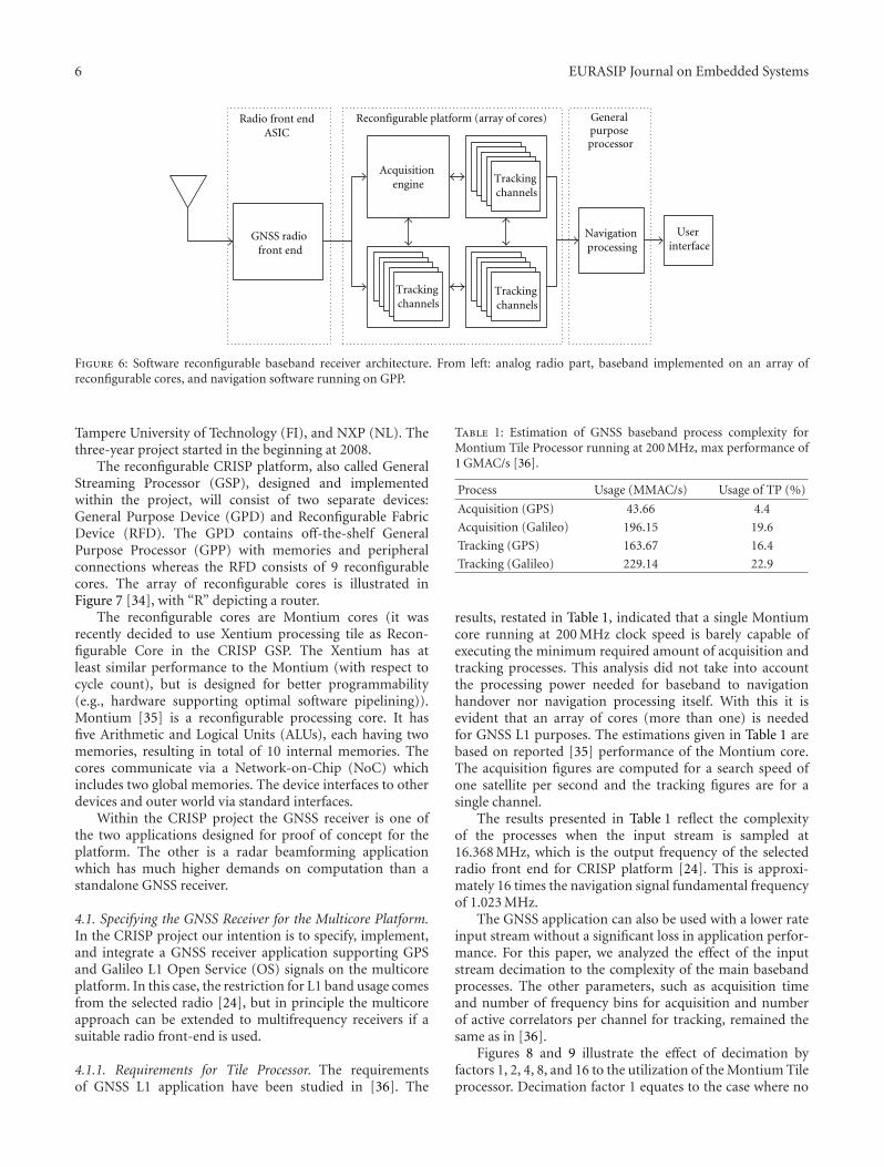
6 EURASIP Journal on Embedded Systems
Navigation processing
Tracking channels
Tracking channels
Tracking channels
Generalpurpose
processor
Reconfigurable platform (array of cores)
User interface
Acquisition engine
Radio front endASIC
GNSS radio front end
Figure 6: Software reconfigurable baseband receiver architecture. From left: analog radio part, baseband implemented on an array ofreconfigurable cores, and navigation software running on GPP.
Tampere University of Technology (FI), and NXP (NL). Thethree-year project started in the beginning at 2008.
The reconfigurable CRISP platform, also called GeneralStreaming Processor (GSP), designed and implementedwithin the project, will consist of two separate devices:General Purpose Device (GPD) and Reconfigurable FabricDevice (RFD). The GPD contains off-the-shelf GeneralPurpose Processor (GPP) with memories and peripheralconnections whereas the RFD consists of 9 reconfigurablecores. The array of reconfigurable cores is illustrated inFigure 7 [34], with “R” depicting a router.
The reconfigurable cores are Montium cores (it wasrecently decided to use Xentium processing tile as Recon-figurable Core in the CRISP GSP. The Xentium has atleast similar performance to the Montium (with respect tocycle count), but is designed for better programmability(e.g., hardware supporting optimal software pipelining)).Montium [35] is a reconfigurable processing core. It hasfive Arithmetic and Logical Units (ALUs), each having twomemories, resulting in total of 10 internal memories. Thecores communicate via a Network-on-Chip (NoC) whichincludes two global memories. The device interfaces to otherdevices and outer world via standard interfaces.
Within the CRISP project the GNSS receiver is one ofthe two applications designed for proof of concept for theplatform. The other is a radar beamforming applicationwhich has much higher demands on computation than astandalone GNSS receiver.
4.1. Specifying the GNSS Receiver for the Multicore Platform.In the CRISP project our intention is to specify, implement,and integrate a GNSS receiver application supporting GPSand Galileo L1 Open Service (OS) signals on the multicoreplatform. In this case, the restriction for L1 band usage comesfrom the selected radio [24], but in principle the multicoreapproach can be extended to multifrequency receivers if asuitable radio front-end is used.
4.1.1. Requirements for Tile Processor. The requirementsof GNSS L1 application have been studied in [36]. The
Table 1: Estimation of GNSS baseband process complexity forMontium Tile Processor running at 200 MHz, max performance of1 GMAC/s [36].
Process Usage (MMAC/s) Usage of TP (%)
Acquisition (GPS) 43.66 4.4
Acquisition (Galileo) 196.15 19.6
Tracking (GPS) 163.67 16.4
Tracking (Galileo) 229.14 22.9
results, restated in Table 1, indicated that a single Montiumcore running at 200 MHz clock speed is barely capable ofexecuting the minimum required amount of acquisition andtracking processes. This analysis did not take into accountthe processing power needed for baseband to navigationhandover nor navigation processing itself. With this it isevident that an array of cores (more than one) is neededfor GNSS L1 purposes. The estimations given in Table 1 arebased on reported [35] performance of the Montium core.The acquisition figures are computed for a search speed ofone satellite per second and the tracking figures are for asingle channel.
The results presented in Table 1 reflect the complexityof the processes when the input stream is sampled at16.368 MHz, which is the output frequency of the selectedradio front end for CRISP platform [24]. This is approxi-mately 16 times the navigation signal fundamental frequencyof 1.023 MHz.
The GNSS application can also be used with a lower rateinput stream without a significant loss in application perfor-mance. For this paper, we analyzed the effect of the inputstream decimation to the complexity of the main basebandprocesses. The other parameters, such as acquisition timeand number of frequency bins for acquisition and numberof active correlators per channel for tracking, remained thesame as in [36].
Figures 8 and 9 illustrate the effect of decimation byfactors 1, 2, 4, 8, and 16 to the utilization of the Montium Tileprocessor. Decimation factor 1 equates to the case where no

EURASIP Journal on Embedded Systems 7
RFD
RR
RRR
R
R R R
Test IF
Chip IF
Chip IF
Channeldata out
RF frontend data
in
Network IF
Reconfigurablecore
Network IF
Reconfigurablecore
Network IF
Reconfigurablecore
Network IF
Reconfigurablecore
Network IF
Reconfigurablecore
Network IF
Reconfigurablecore
Network IF
Reconfigurablecore
Network IF
Reconfigurablecore
Network IF
Reconfigurablecore
Smartmemory
Smartmemory
Parallel IF
Parallel IF
Parallel IF
Parallel IF
JTAG
Serial IF
Serial IF
Serial IF
Tracking channel 3
Tracking channel 4Tracking channel 1
Tracking channel 2 Tracking channel 5
Tracking channel 0
Acquisition 0
Serial IF
Figure 7: Array of 9 reconfigurable cores [34] with example mapping of GNSS application illustrated, the selection of cores is random. “R”depicts router and “IF” interface.
decimation is applied, that is, results shown in Table 1. Thepresented figures show how the complexity of both processes,measured as Montium Tile Processor utilization percentage,decreases exponentially as decimation factor increases. Thebehavior is the same for GPS and Galileo signals, except thatutilization with Galileo signals is a bit larger than with GPSin all studied cases.
To ease the computational load of the Tile Processor thedecimation of the input stream seems to be a feasible choice.The amount of decimation should be sufficient to effectmeaningful savings in TP utilization without significantlydegrading performance of the application. For the currentGPS SPS signal, decimation by factor 4 (4.092 MHz) isfeasible without significant loss in receiver performance.Factor of 8 (2.046 MHz) is equal to the Nyqvist rate for1.023 MHz, which is the PRN code rate used in GSP SPSsignal.
In the Galileo case, decimation factor 4 is the maximumdecimation factor. This is because with a sampling frequencyof approximately 4 MHz the BOC(1,1) component of theGalileo E1 OS signal can be still received with a maximumloss of only −0.9 dB, when compared with the reception ofthe whole MBOC bandwidth [12]. (This applies also to themodern GPS L1C signals, but they are not specified in ourapplication [36].)
Table 2: Estimation of GNSS baseband process complexity withdecimated (by factor 4) input stream. Montium Tile Processorrunning at 200 MHz, max performance of 1 GMAC/s.
Process Usage (MMAC/s) Usage of TP (%)
Acquisition (GPS) 9.57 0.96
Acquisition (Galileo) 43.66 4.37
Tracking (GPS) 40.92 4.09
Tracking (Galileo) 57.28 5.73
In the ideal case the decimation of the input streamshould be changing with the receiver mode (GPS/Galileo).Since in CRISP the decimation of the radio stream will beimplemented as hardware in FPGA, which is connecting theradio to the parallel interface of the final CRISP prototypeplatform, the run time configuration of the decimation factoris not feasible. For this reason, in the rest of the paper we willfocus on the scenario where fixed decimation factor of 4 isused, resulting in a stream sample rate of 4.092 MHz.
Table 2 shows baseband complexity estimation for thecase when input stream is decimated by a factor of four.When it is compared to the original figures of complexityshown in Table 2, it can be seen that the utilization of TPis over four times smaller.

8 EURASIP Journal on Embedded Systems
2 4
GPSGalileo
Input stream decimation factor
6 8 1210 14 160
4
6
2
8
10
Mon
tiu
m t
ile p
roce
ssor
uti
lizat
ion
(%
)
12
14
16
18
20
Figure 8: Acquisition process utilization of Montium Tile Processorresources as a function of the decimation factor of the input stream.
2 4
GPSGalileo
Input stream decimation factor
6 8 1210 14 160
5
10
Mon
tiu
m t
ile p
roce
ssor
uti
lizat
ion
(%
)
15
20
25
Figure 9: Tracking process utilization of Montium Tile Processorresources as a function of the decimation factor of the input stream.
4.1.2. Requirements for the Network-on-Chip. To analyze themulticore GNSS receiver application we built a functionalsoftware receiver with the C++ language, running on a PC.The detailed analysis of the software receiver will be given insubstantial paper [37].
In our SW receiver each process was implemented as asoftware thread. With approximating one process per corethis approach enabled us to estimate the link payload bylogging communication between the threads.
We estimated a scenario where one core was allocatedto perform acquisition and six cores were mapped for thetracking process. This scenario is illustrated in Figure 7. Dig-itized RF front-end data is input to the NoC via an interface.
40004100
430044004500
4200
Payl
oad
(byt
es/m
s)
0 0.5 1
Time (ms)
1.5 2 2.5 3.53 4.54 5×10³
(a) Acquisition link payload
40904095
410541104115
4100
Payl
oad
(byt
es/m
s)
0 0.5 1
Time (ms)
1.5 2 2.5 3.53 4.54 5×10³
(b) Average tracking link payload
Figure 10: Link payloads for GPS acquisition process (a) andaverage payload of GPS tracking processes (b).
A specific chip interface is used to connect the RFD to theGPD, and it is used to forward channel data (channel phasemeasurement data related to pseudorange measurements,and navigation data) to the GPD. The Selected mappingis a compromise between minimal operative setup (oneacquisition and four tracking) and the needs of dependabilitytesting processes, where individual cores may be taken offlinefor testing purposes.
The scenario was simulated with a prerecorded set ofreal GPS signals. Since signal sources for Galileo navigationwere not available, the Galileo case was not tested. Thelink payloads caused by the cores communicating while thesoftware was running for 5 seconds is illustrated in Figure 10.
The results show that, in GPS mode, our GNSS appli-cation causes a payload for each link/processing core with aconstant baseline of 4096 Bytes/millisecond. This is causedby the radio front-end input, that is, the incoming signal.In this scenario we used real GPS front end data which wassampled at 4.092 MHz, each byte representing one sample.This sampling rate is also equal to the potential decimationscenario discussed earlier.
With a higher sampling rate the link payload baseline willbe raised, but on the other hand one byte can be preprocessedto contain more than one sample, decreasing the trafficcaused by radio front-end input.
The first peak in the upper part of Figure 8 is causedby the acquisition process output. When GNSS applicationstarts, FFT-based acquisition is started and the results areready after 60 milliseconds, which are then transmitted totracking channels. This peak is also the largest individualpayload event caused by the GNSS application.
After a short initialization period the tracking processesstart to produce channel output. An Average of simulatedGPS tracking link/processing core payloads is illustratedin Figure 10(b). Every 20 milliseconds a navigation datasymbol (data rate is 50 Hz in GPS) is transmitted and oncea second higher transmission peak is caused by the loop

EURASIP Journal on Embedded Systems 9
phase measurement data, which is transmitted to GPD forpseudorange estimation.
In Galileo mode, the payload caused by incoming signalwill be equal since the same radio input will be used forboth GPS and Galileo. However, the transmission of datasymbols will cause a bigger payload since data rate of GalileoE1 signals is 250 symbols per second [8]. Galileo phasemeasurement rate will remain the same as in GPS mode.
From the results it is seen that the link payload caused bythe incoming RF signal is the largest one in both operatingmodes, and if the link payload needs to be optimized thereduction of it is the first thing to be studied. The results alsoindicate that when GNSS application is running smoothlythe link payloads caused by it are predictable.
Note that this estimation does not contain any over-heads caused by network protocol or any other data thannavigation related (dependability, real-time mapping of theprocesses). These issues will be studied in our future work.
4.2. Open Issues. Besides the additional network load causedby other than the GNSS application itself, there are alsosome other issues that remain open. There may be challengesin designing software for a multicore environment. Powerconsumption as well as the final bill of materials (BOMs),(i.e., final price of the multicore product) remains an openissue at the time of this writing. In future these issues willbe studied and suitable optimizations performed after theprototyping and proof of concepts have been completedsuccessfully.
5. Conclusions
In this paper we discussed three Software-Defined Radio(SDR) architectures for a Global Navigation Satellite System(GNSS) receiver. The usage of flexible architectures inGNSS receiver was justified with the need for implementingsupport for upcoming navigation systems and new algo-rithms developed, and especially for multipath mitigation.The hardware accelerated SDR architecture is quite closeto the current mass market solutions. There the ASIC isreplaced with a reconfigurable piece of hardware, usually anFPGA. The second architecture, ideal (or pure) SDR receiveris using a single processor to realize all necessary signalprocessing functions. Real-time receivers remain a challenge,but postprocessing applications are already taking advantageof this architecture.
The third architecture, SDR with multiple cores, is anovel approach for GNSS receivers. This approach benefitsin both having high degree of flexibility, and when properlydesigned and scaled, a reasonably low unit price in highvolume production. In this paper we also presented theCRISP project where such a multicore architecture willbe realized along with the analysis of GNSS applicationrequirements for the multicore platform.
We extended the previously published analysis of pro-cessing tile utilization to cover the effect of input streamdecimation. Decimation by factor four seems to offer agood compromise between core utilization and applicationperformance.
We implemented a software GNSS receiver with processesimplemented as threads and used that to analyze the GNSSapplication communication payload for individual links.This analysis indicated that the incoming signal representsthe largest part of the communication in the networkbetween processing cores.
Acknowledgments
The authors want to thank Stephen T. Burgess from TampereUniversity of Technology for his useful comments aboutthe manuscript. This work was supported in part by theFUGAT project funded by the Finnish Funding Agency forTechnology and innovation (TEKES). Parts of this researchare conducted within the FP7 Cutting edge ReconfigurableICs for Stream Processing (CRISP) project (ICT-215881)supported by the European Commission.
References
[1] E. D. Kaplan and C. J. Hegarty, Eds., Understanding GPS,Principles and Applications, Artech House, Boston, Mass, USA,2nd edition, 2006.
[2] J. Benedicto, S. E. Dinwiddy, G. Gatti, R. Lucas, and M.Lugert, “GALILEO: Satellite System Design and TechnologyDevelopments,” European Space Agency, November 2000.
[3] S. Revnivykh, “GLONASS Status and Progress,” Decem-ber 2008, http://www.oosa.unvienna.org/pdf/icg/2008/icg3/04.pdf.
[4] G. Gibbons, “International system providers meeting (ICG-3) reflects GNSS’s competing interest, cooperative objectives,”Inside GNSS, December 2008.
[5] U. S. Airforce, “GPS Modernization Fact Sheet,” 2006,http://pnt.gov/public/docs/2006/modernization.pdf.
[6] M. S. Braasch and A. J. van Dierendonck, “GPS receiverarchitectures and measurements,” Proceedings of the IEEE, vol.87, no. 1, pp. 48–64, 1999.
[7] K. Borre, D. M. Akos, N. Bertelsen, P. Rinder, and S. H.Jensen, A Software Defined GPS and Galileo Receiver—ASingle-Frequency Approach, Birkhauser, Boston, Mass, USA,2007.
[8] “Galileo Open Service, Signal in space interface controldocument (OS SIS ICD),” Draft 1, February 2008.
[9] “Interface Specification—Navstar GPS Space segment/Usersegment L1C Interfaces,” IS-GPS-800, August 2007.
[10] R. D. Fontana, W. Cheung, and T. Stansell, “The modernizedL2C signal—leaping forward into the 21st century,” GPSWorld, pp. 28–34, September 2001.
[11] “Galileo Joint Undertaking—Galileo Open Service, Signal inspace interface control document (OS SIS ICD),” GJU, May2006.
[12] G. W. Hein, J.-A. Avila-Rodriguez, S. Wallner, et al., “MBOC:the new optimized spreading modulation recommendedfor GALILEO L1 OS and GPS L1C,” in Proceedings ofthe IEEE/ION Position, Location, and Navigation Symposium(PLANS ’06), pp. 883–892, San Diego, Calif, USA, April 2006.
[13] H. Hurskainen, E. S. Lohan, X. Hu, J. Raasakka, and J. Nurmi,“Multiple gate delay tracking structures for GNSS signalsand their evaluation with simulink, systemC, and VHDL,”International Journal of Navigation and Observation, vol. 2008,Article ID 785695, 17 pages, 2008.

10 EURASIP Journal on Embedded Systems
[14] S. Kim, S. Yoo, S. Yoon, and S. Y. Kim, “A novel unambiguousmultipath mitigation scheme for BOC(kn, n) tracking inGNSS,” in Proceedings of the International Symposium onApplications and the Internet Workshops, p. 57, 2007.
[15] F. Dovis, M. Pini, and P. Mulassano, “Multiple DLL archi-tecture for multipath recovery in navigation receivers,” inProceedings of the 59th IEEE Vehicular Technology Conference(VTC ’04), vol. 5, pp. 2848–2851, May 2004.
[16] F. Dovis, A. Gramazio, and P. Mulassano, “SDR technologyapplied to Galileo receivers,” in Proceedings of the InternationalTechnical Meeting of the Satellite Division of the Institute ofNavigation (ION GPS ’02), Portland, Ore, USA, September2002.
[17] “SDR Forum,” January 2009, http://www.sdrforum.org.[18] J. Mitola, “The software radio architecture,” IEEE Communi-
cations Magazine, 1995.[19] P. G. Mattos, “A single-chip GPS receiver,” GPS World, October
2005.[20] P. J. Mumford, K. Parkinson, and A. G. Dempster, “The
namuru open GNSS research receiver,” in Proceedings of theInternational Technical Meeting of the Satellite Division of theInstitute of Navigation (ION GNSS ’06), vol. 5, pp. 2847–2855,Fort Worth, Tex, USA, September 2006.
[21] S. Ganguly, A. Jovancevic, D. A. Saxena, B. Sirpatil, and S.Zigic, “Open architecture real time development system forGPS and Galileo,” in Proceedings of the International TechnicalMeeting of the Satellite Division of the Institute of Navigation(ION GNSS ’04), pp. 2655–2666, Long Beach, Calif, USA,September 2004.
[22] H. Hurskainen, T. Paakki, Z. Liu, J. Raasakka, and J. Nurmi,“GNSS receiver reference design,” in Proceedings of the 4thAdvanced Satellite Mobile Systems (ASMS ’08), pp. 204–209,Bologna, Italy, August 2008.
[23] J. Hill, “Navigation signal processing with FPGAs,” in Pro-ceedings of the National Technical Meeting of the Institute ofNavigation, pp. 420–427, June 2004.
[24] Atmel, “GPS Front End IC ATR0603,” Datasheet, 2006.[25] M. Detratti, E. Lopez, E. Perez, and R. Palacio, “Dual-
frequency RF front end solution for hybrid Galileo/GPSmass market receiver,” in Proceedings of the IEEE ConsumerCommunications and Networking Conference (CCNC ’08), pp.603–607, Las Vegas, Nev, USA, January 2008.
[26] P. Fine and W. Wilson, “Tracking algorithms for GPS offsetcarrier signals,” in Proceedings of the ION National TechnicalMeeting (NTM ’99), San Diego, Calif, USA, January 1999.
[27] H. Hurskainen and J. Nurmi, “SystemC model of an interop-erative GPS/Galileo code correlator channel,” in Proceedings ofthe IEEE Workshop on Signal Processing Systems (SIPS ’06), pp.327–332, Banff, Canada, October 2006.
[28] D. M. Akos, “The role of Global Navigation Satellite System(GNSS) software radios in embedded systems,” GPS Solutions,May 2003.
[29] C. Dionisio, L. Cucchi, and R. Marracci, “SOFTREC G3,software receiver and signal analysis fog GNSS bands,” inProceedings of the 10th IEEE Internationl Symposium on SpreadSpectrum Techniques and Applications (ISSSTA ’08), Bologna,Italy, August 2008.
[30] G. E. Moore, “Cramming more components onto integratedcircuits,” Proceedings of the IEEE, vol. 86, no. 1, pp. 82–85,1998.
[31] S. Soderholm, T. Jokitalo, K. Kaisti, H. Kuusniemi, andH. Naukkarinen, “Smart positioning with fastrax’s softwareGPS receiver solution,” in Proceedings of the InternationalTechnical Meeting of the Satellite Division of the Institute of
Navigation (ION GNSS ’08), pp. 1193–1200, Savannah, Ga,USA, September 2008.
[32] J. H. Won, T. Pany, and G. W. Hein, “GNSS software definedradio: real receiver or just a tool for experts,” Inside GNSS, pp.48–56, July-August 2006.
[33] “CRISP Project,” December 2008, http://www.crisp-project.eu.
[34] P. Heysters, “CRISP Project Presentation,” June 2008,http://www.crisp-project.eu/images/publications/D6.1CRISP project presentation 080622.pdf.
[35] P. M. Heysters, G. K. Rauwerda, and L. T. Smit, “A flexible,low power, high performance DSP IP core for programmablesystems-on-chip,” in Proceedings of the IP/SoC, Grenoble,France, December 2005.
[36] H. Hurskainen, J. Raasakka, and J. Nurmi, “Specification ofGNSS application for multiprocessor platform,” in Proceedingsof the International Symposium on System-on-Chip (SOC ’08),pp. 128–133, Tampere, Finland, November 2008.
[37] J. Raasakka, H. Hurskainen, and J. Nurmi, “Modeling multi-core software GNSS receiver with real time SW receiver,”in Proceedings of the International Technical Meeting of theSatellite Division of the Institute of Navigation (ION GNSS ’09),Savannah, Ga, USA, September 2009.


Publication 7
c©2009 IEEE. Reprinted, with permission, from Proceedings of the IEEEWorkshop on Signal Processing Systems Design and Implementation (SIPS),“Optimal Dual Frequency Combination for Galileo Mass Market ReceiverBaseband”, Heikki Hurskainen, Elena-Simona Lohan, Jari Nurmi, StephanSand, Christian Mensing, and Marco Detratti.
This material is posted here with permission of the IEEE. Such permission of theIEEE does not in any way imply IEEE endorsement of any of the Tampere Universityof Technology’s products or services. Internal or personal use of this material ispermitted. However, permission to reprint/republish this material for advertising orpromotional purposes or for creating new collective works for resale or redistributionmust be obtained from the IEEE by writing to [email protected].
By choosing to view this material, you agree to all provisions of the copyright lawsprotecting it.

OPTIMAL DUAL FREQUENCY COMBINATION FOR GALILEO MASS MARKETRECEIVER BASEBAND
Heikki Hurskainen†, Elena-Simona Lohan‡, Jari Nurmi†, Stephan Sand�,Christian Mensing�, and Marco Detratti∗
†Tampere Univ. of Technology, Dept. of Computer Systems/ ‡Dept. of Communications Engineering,P.O. Box 553, FI-33101, Tampere, FINLAND
�German Aerospace Center (DLR), Institute of Communications and Navigation,Oberpfaffenhofen, 82234 Wessling, GERMANY
∗ACORDE TECHNOLOGIES S.A., Centro de Desarrollo Tecnologico,Avda. de los Castros s/n, 39005 Santander, SPAIN
ABSTRACTGRAMMAR (EC FP7) is a project aiming to deliver IPfor future Galileo mass market receivers. One of the out-comes of this project will be an advanced Galileo receiverprototype. In this paper we present the research for findingthe optimal dual frequency option for a Galileo mass mar-ket receiver. We discuss the impact of multiple frequencieson baseband algorithms and the implementation issues ofa dual-frequency baseband. From the analysis results, wedraw the following conclusions: E1/E5a combination is theoptimal dual-frequency solution for Galileo; a common dual-frequency baseband architecture with flexible channels seemsto be the best implementation approach for a Galileo E1/E5adual-frequency receiver.
1. INTRODUCTION
Galileo Ready Advanced Mass MArket Receiver (GRAM-MAR), is a 2-year project focusing on advanced Galileo re-ceiver technology for mass market segment. The consortiumis comprised of the German Aerospace Center (DLR), whichis the coordinator, ACORDE, which is a Spanish radio fre-quency (RF) design SME, and Tampere University of Tech-nology from Finland.
GRAMMAR aims to boost the Galileo downstream in-dustry by taking the effort to provide IP for future Galileomass market receivers. One of the project outcomes will be anadvanced Galileo mass market receiver prototype. This pro-totype can receive multiple frequencies extending the work ofGRAMMAR beyond state-of-the-art single frequency massmarket receivers.
Currently, only high-end professional receivers exploitmultiple frequencies. While additional complexity and power
The research leading to these results has received funding from the Euro-pean Community’s Seventh Framework Programme (FP7/2007-2013) underthe GRAMMAR project, grant agreement n◦ 227890.
consumption is uncritical for this receiver segment, the benefitis increased accuracy due to ionospheric delay error correc-tion, better multipath and interference resilience, and largersignal bandwidth.
GRAMMAR aims at transferring the multiple-frequencytechnology from high-end receivers to mass market receiverswhile providing the benefits but solving the complexity andpower consumption issues.
2. FUTURE GALILEO FREQUENCY BANDS
The Galileo system will operate at four frequency bands; E5a,E5b, E6 and E1 bands. Bands are illustrated in Figure 1. Asseen in Figure 1, there are two bands shared between Galileoand Global Positioning System (GPS), E5a/L5 and E1/L1.
Since the E6 band does not offer open service (OS) signals[1], it is not considered as alternative for Galileo mass marketreceivers. This leaves three dual Galileo frequency options tobe studied;
• E1/E5a (overlapping with GPS signals),
• E1/E5b, and
• E1/E5 (E5a and E5b signals are part of the E5 signal inits full bandwidth).
The signal characteristics for applicable Galileo OS sig-nals are listed in Table 1.
2.1. Interference issues
Two types of interference are present in a multi-frequency re-ceiver; inter-system interference caused by other system’s sig-nals (e.g. Galileo/GPS) and intra-system interference causedby signals from same system (e.g. Galileo E1/E5).
Regarding the intra-system interference, the most criticalcase is when we select a common baseband architecture for
261978-1-4244-4335-2/09/$25.00 ©2009 IEEE SiPS 2009

Table 1. Signal characteristics for Galileo OS signals [1].Band fcarr [MHz] BW [MHz] Code length Rate [chips/ms] Modulation type
E1 1575.420 24.552 4092 1023 CBOCE5 1191.795 51.150 N/A 10230 AltBOC(15,10) of E5a & E5bE5a 1176.450 20.460 10230 10230 BPSKE5b 1207.140 20.460 10230 10230 BPSK
Fig. 1. Future Galileo and GPS Frequency Plan [1]
both frequencies: in this situation, both signals (e.g. E1/E5a,etc) are down-converted to the same low intermediate fre-quency (IF); the interference level is determined in a greatmeasure by the modulation combinations. In order to mea-sure the amount of interference between two signals, a typicalmeasure is the spectral separation coefficient (SSC) [2], [3].SSC between two signals within a complex finite bandwidthBW is defined similar to [3], as:
SSC =∫ BW/2
−BW/2
PSD1(f)PSD2(f)df (1)
Where PSD1 and PSD2 are the normalized power spec-tral densities of the 2 interfering signals (if PSD1 = PSD2,then we have self interference). The normalization is done insuch a way that
∫ ∞−∞ PSDi(f)df = 1, i = 1, 2.
The expressions for PSDs for binary phase-shift keying(BPSK), multiplexed binary offset carrier (MBOC) and alter-native BOC (AltBOC)-modulated signals can be found in [3],[4], and [5]. The lower the SSC is, the better spectral separa-tion is between the signals.
The SSC values for different signal combinations, assum-ing that they all have been down-converted to baseband, areshown in Table 2. The SSC values with E5 signal are ratherlow at low BW only because the signal main lobes are notcaptured in the considered bandwidth. From Table 2, we cansee that the SSC of E1, E5a and E5b self-interference varyvery little or at all with the increase of bandwidth above 13MHz. We also notice that the SSC is about 20 dB better be-tween E1 and E5 than between E1 and E5a (or between E1and E5b).
This means, that from the point of view of intra-system
interference, it might be more advantageous to use E1/E5combination. However, the drawback is the need of a muchhigher receiver bandwidth and sampling frequencies. There-fore more complex baseband processing is required and thus,more power is consumed. The gain in terms of interference isprobably not enough to justify the loss in terms of power con-sumption. Moreover, since in a 51.15 MHz bandwidth for E5signal there is only about 73% of the signal power (as it willbe shown later on in this paper), we also expect a degradationof acquisition and tracking performances for E5 signals.
The self-interference level is comparable for E5a/E5b andE5 signals. From the interference point of view, the leastamount of interference seems to be given by the E1/E5b com-bination.
3. RECEIVER BASEBAND ALGORITHMS
The fundamental satellite navigation receiver contains threedomains; analog signal processing, digital signal processing,and navigation [6], [7]. Analog signal processing refers to theradio part, in this paper we assume two radios to be used indual frequency receiver, one for each frequency. Studies fordual frequency radio front-ends are available in literature, e.g.in [8] and [9], but the detailed analysis of multi-frequency is-sues in the radio domain is out of the scope of this paper. Theimportant characteristic of radio is how the analog to digi-tal conversion is handled. The sampling frequency affects thequality of received signals as discussed in the next subsection.
After analog to digital conversion the digital signal pro-cessing, a.k.a. baseband processing, takes place. The mainfunctions in the baseband are to find the signals totally buriedin noise and when found, keep the synchronization betweenreceiver and signal to demodulate the low rate navigation dataand to measure pseudoranges. The first function is called asacquisition and the latter as tracking.
The last functional domain of the receiver is navigation,where the receiver’s Position, Velocity and Time (PVT) is es-timated. The computation is using multi-lateration methodsbased on the measured distances between receiver and satel-lites (pseudoranges) and known locations of satellites.
3.1. Sampling frequency effects
The signal modulation defines the minimum required band-width for certain power containment. The power containment
262

Table 2. Spectral separation coefficients (SSC) between different combinations of signals (including self-interference) forGalileo signals and different receiver bandwidths BW; in dB-Hz
BW [MHz] E1/E1 E1/E5a and E1/E5b E1/E5 E5a/E5a and E5b/E5b E5/E5
13 -65.85 -81.07 -115.53 -92.10 -150.6220.46 -65.85 -81.05 -111.05 -92.07 -118.11
24.552 -65.85 -81.05 -108.32 -92.06 -109.1526 -65.85 -81.05 -107.87 -92.06 -106.79
51.15 -65.85 -81.05 -101.31 -92.05 -97.73
is the percentage of the signal power contained within a cer-tain bandwidth and it is directly related to the demodulationand tracking properties of the signal. For instance, the smallerthe bandwidth needed for a certain power containment, thebetter the bandwidth efficiency that can be achieved. Moredetails can be found, e.g. in [3]. The power containment for3 different bandwidths and for E1 and E5/E5a/E5b signalsis shown in Table 3. The first 2 double-sided bandwidths of13 MHz and 26 MHz, respectively, are selected according tocommon GSM crystal frequencies [10]. The third BW usedhere is the recommended bandwidth in [1].
Clearly, with proposed sampling frequencies the E1/E5combination is not feasible, because there will be not enoughsignal energy captured in the processed bandwidth. Only13.05% of the signal power is contained within 26 MHzdouble-sided bandwidth. The other 2 combinations, namelyE1/E5a and E1/E5b, are feasible with both 13 MHz and 26MHz sampling frequencies.
Table 3. Power containment (in percentage) per bandwidthBW [MHz] E1 E5a/E5b E5
13 92.88% 85.66% 0.08%26 96.11% 91.10% 13.05%
BW from SIS-ICD [1] 96.04% 90.28% 73.32%
The power containment factor versus bandwidths is il-lustrated in Figure 2. The minimum bandwidth requirement(double-sided bandwidth) for a power containment of at least90% are 12.1 MHz (E1), 17.4 MHz (E5a/E5b), and 156.6MHz (E5). This is equal with the minimum sampling fre-quency needed for at least 90 % power containment.
3.2. Impact on Acquisition
Following factors are dominating the acquisition stage formulti-frequency receiver. As shown in Table 1 multi-frequencysignals have different spreading codes, with different lengthsand speed rates, and also different modulation types.
The modulation types affect the shape of the correla-tion functions. An example is shown in Figure 3, for theideal envelope of the auto-correlation function (ACF) for E1,E5a/E5b and E5 signals. The more ambiguities (i.e., deepfades) in the ACF envelope are present, the more difficult
0 10 20 30 40 50 60 700
10
20
30
40
50
60
70
80
90
100
Signal double−sided baseband bandwidth [MHz]
Power containment versus bandwidth
Pow
er c
onta
inm
ent (
%)
E1E5a/E5bE5
Fig. 2. Power containment versus bandwidth for Galileo.
(i.e., complex) is the acquisition process. From this point ofview, the E5a/E5b signals are the easiest to acquire, while theE5 signals are the most complex. The complexity also de-pends on the primary code length: the higher the code length,the more complex the acquisition process becomes. Fromthis point of view, E1 signals are the simplest to acquire, andE5a, E5b and E5 signals have the same code lengths.
By analogy with the GPS case, where a step of 0.5 chips(GPS L1 signal’s chip rate is 1023 chips/ms, so this approxi-mates 489 ns) is used in acquisition process [7], it follows thata good rule of thumb about setting the step of the time bin hy-potheses in the acquisition process (when ambiguous acqui-sition methods are used) might be to take this step equal to aquarter of the main lobe width of the ACF envelope. Basedon Figure 3, we can easily compute that a minimum step of0.175 chips (171 ns) is needed to acquire E1 signal (with clas-sical ambiguous methods), a minimum step of 0.5 chips (49ns) is needed for E5a and E5b signals, and a minimum step of0.0833 chips (8 ns) is needed for E5 signal.
The number of timing hypotheses per frequency bin, fora full time search (i.e., unassisted acquisition) is equal to theprimary code length divided by the minimum time-bin step.This number is illustrated in Table 4. Based on this exam-ple, signals E1 and E5a/E5b have similar complexity in the
263

−1 −0.5 0 0.5 10
0.1
0.2
0.3
0.4
0.5
0.6
0.7
0.8
0.9
1
Delay error [chips]
norm
aliz
ed A
CF
enve
lope
ACF shapes
E1E5a/E5bE5
Fig. 3. Normalized envelope of the ACF for the 3 modulationtypes used in OS Galileo: CBOC (E1 signal), BPSK (E5a andE5b signals) and AltBOC(15,10)(E5 signal).
acquisition process (at least when ambiguous or classical ac-quisition is employed), while the E5 signal is about 5 timesmore complex to be acquired. A detailed explanation of am-biguous and unambiguous acquisition methods can be foundin [11].
To ease the processing needed acquisition informationfrom E1 band signal can be used for acquiring signals fromE5 band also, since the E1 and E5 signals are synchronizedin transmission.
Table 4. Number of timing hypotheses per frequency bin inthe acquisition process for Galileo OS signals.
E1 E5a and E5b E5
23383 20460 122810
3.3. Impact to Tracking
From the point of view of tracking process, the following is-sues have an impact on the tracking complexity; The samplingfrequency, which is the highest when a combination based onE5 is used as was discussed earlier. The number of correlatorsin the tracking channel, since the number of needed correlatoris modulation dependent. For example, if multiple gate delay(MGD) [12] structures are to be used, the optimal parameters,such as weighting factors and number of gates depend on themodulation type.
Tracking is based on usage of locked loops for signaldelay (DLL), phase (PLL), and frequency (FLL). The band-width of the loops is depending on the modulation. Thus,a multi-frequency receiver needs re-configurable loops formulti-frequency reception.
From the point of view of multipath mitigation, E1/E5 areseparated by roughly 350 MHz, which means that we havemore likely some independent amplitudes and phases of mul-tipath components. Moreover, E5 signals with larger band-width and different modulation types may provide better mul-tipath resistance than E1 signals, therefore, from multipathpoint of view, E1/E5 combination might prove the best alter-native.
From the point of view of coherent data integration, thecoherent integration length in non-pilot channels is limitedby the presence of data bits. Since in E5a, the navigationdata rate is 50 bps and in E5b the navigation data rate is 250bps, it follows that E5a is better than E5b from the point ofcoherent integration (larger coherent integration can be madewith smaller data navigation rate).
3.4. Comparison of various dual-frequency variants
Table 5 summarize all the advantages and disadvantages ofvarious dual-frequency combinations, as discussed above. Inthis Table, a ’+’ stands fr the best variant among the 3 pos-sibilities (if 2 variants have identical performance, then bothappear with ’+’ sign) and a ’-’ sign stands for the other vari-ants. Clearly, from this table (by choosing the variant with themaximum number of ’+’s), the best dual-frequency choice isE1/E5a combination.
Table 5. Comparison of dual-frequency variants according tovarious criteria.
Criterion E1/E5a E1/E5b E1/E5
acq. time + + -intra-syst. interf - - +inter-syst. interf - + -power containm. + + -coh. integr. + - -multipath mitig. - - +best compatibility + - -with GPS
4. DUAL FREQUENCY BASEBANDIMPLEMENTATION ISSUES
4.1. Dual frequency baseband architectures
Two options for multi-frequency baseband architecture for fu-ture mass market receivers are foreseen; either using a com-mon baseband for all received frequencies or a dual/multibaseband option with merging signals at navigation layer.These architectures are illustrated in Figures 4(a) and 4(b).
In the dual single-frequency baseband architecture (Fig-ure 4(a)) each selected frequency band has its own basebandhardware. With this approach the baseband can be tailored
264

(a) Dual single-frequency basebands
(b) Common dual-frequency baseband
Fig. 4. Dual-frequency architectures. RF refers to receivedsignal, IF to down-converted digital signal stream (radio out-put) and ρ to pseudorange measurement.
for the selected frequency band. On the other hand the num-ber of dedicated baseband channels to each frequency is fixed.Thus, resources may be wasted if the available satellite sce-nario is not transmitting good signals in all frequencies ,i.e.,some channels remain unused.
In this architecture the baseband units need to be synchro-nized. This makes it possible to forward the acquisition infor-mation, i.e., estimates of code delays and Doppler frequen-cies, from one band to another. Both baseband units are tak-ing input from the RF front end dedicated to that frequency.
The common dual-frequency baseband architecture (Fig-ure 4(b)) is more flexible with different scenarios. Since thesame baseband is capable of processing both bands it canadapt to surrounding signal environment much better. To al-low the reception of two radio IF outputs to a single base-band the IF signals should be synchronized at sample level(i.e. synchronized sampling).
The baseband is containing a dedicated acquisition en-gine; an entity that seeks satellite signals from received noise.Baseband is also containing a number of flexible trackingchannels. When channel is synchronized with incoming sig-nal, i.e., tracking is locked, the tracking channel can extractnavigation data out of received stream and also perform mea-surements to estimate the pseudorange.
4.2. Input signal management
In architecture illustrated in Figure 4(b), the IF output fromtwo radios needs to be inserted to a single baseband. Ourimplementation approach for inserting dual radio signal to asingle flexible tracking channel is illustrated in Figure 5. A
Multiplexer (MUX) is used, the type of input is selected (Sel)by the software controller. One must take a note that thisimplementation assumes the sampling rates of two inputs tobe synchronized.
Fig. 5. Implementation detail for radio source selection. IFrefers to digital IF signal stream and ρ to a single channelpseudorange data output.
4.3. Acquisition implementation
Basically, only E1/L1 needs to implemented since this infor-mation can be used for E5a/L5 delay and Doppler estimation.E1 signal acquisition is more feasible for implementation dueit’s lower code speed. This decision will also decrease thecomplexity of the final baseband design.
4.4. Tracking implementation
As mentioned, baseband contain number of tracking chan-nels, each capable of processing one signal at time. A genericoverview of a flexible tracking channel is given in Figure 6.Each channel consists of a set of blocks that are reusable fordifferent signals/frequencies, such as numerically controlledoscillators (NCOs), correlators, accumulators, and another setthat are frequency/signal specific, e.g., local sub-carrier andcode sources.
Three main sub-processes can be identified on the sig-nal chain through tracking channel. In the carrier wipe-offprocess the IF and Doppler frequencies are removed from re-ceived IF signal. The frequency of local copy of IF signal issoftware controllable via Numerically Controlled Oscillator(NCO).
In the next process the received signal’s sub-carrier (mod-ulation) is removed by correlating it with local copy. Thesource for local sub-carrier is selected with a MUX, whichis also controlled by the receiver software. In code wipeoff(or correlation) the incoming signal is correlated with severalversions of local copy of the PRN code with different delays.Again, the source of the PRN (memory codes for E1 and codegenerator for E5a [1]) is selectable via MUX. The correlationresults are accumulated (integrated) over a predefined periodof time. Integration time depends on the PRN code length,speed rate and requirements set for the receiver sensitivity.
Besides that the flexible tracking channel approach iscapable of processing signals from two frequency bands, itcan be also utilized to multi-system reception. Galileo and
265

Fig. 6. Structure for a generic flexible tracking channel.
GPS signals have same fundamental structure in shared bands(E1/L1 and E5a/L5), so Galileo tracking channel can be usedfor GPS with replacing local modulation and PRN genera-tion. This would mean an additional input to the MUXespresented in Figure 6.
5. CONCLUSION
From the presented work, it can be seen that the E1/E5 com-bination is much more complex than E1/E5a or E1/E5b com-bination. Because the focus is on mass-market receivers, webelieve E1/E5 combination is not a viable solution for mass-market dual-frequency receiver. The other two possible com-binations, namely E1/E5a and E1/E5b have similar character-istics in terms of acquisition, tracking and interference level(with small differences regarding coherent integrations andthe inter-system interference). The E1/E5a combination hasthe additional property that it overlaps exactly with GPS fre-quency band L1 and L5. This property confers the advantageof an easier integrability of a joint Galileo/GPS receiver. Be-ing taken all the discussed criteria into account, we believethat E1/E5a combination is the best dual-frequency solutionfor Galileo mass-market receiver.
In terms of our recommendation for preferred basebandarchitecture, a common dual-frequency baseband architecturewith flexible channels (decision making implemented by soft-ware) seems to be the best option. This approach would alsomaximize the re-usability, thus minimizing the cost, of base-band hardware components.
6. REFERENCES
[1] “Galileo Open Service, Signal in space interface controldocument (OS SIS ICD),” Feb 2008, Draft 1.
[2] J.W. Betz, “The Offset Carrier Modulation for GPSmodernization,” in Proc. of ION Technical meeting,Cambridge, Massachusetts, Jun 1999, pp. 639–648.
[3] E. S. Lohan, A. Lakhzouri, and M. Renfors, “Binary-Offset-Carrier modulation techniques with applicationsin satellite navigation systems,” Wiley InternationalJournal of Wireless Communications and Mobile Com-puting, DOI: 10.1002/ wcm.407, Jul 2006.
[4] E.S. Lohan, A. Lakhzouri, and M. Renfors, “ComplexDouble-Binary-Offset-Carrier modulation for a unitarycharacterization of Galileo and GPS signals,” IEEE Pro-ceedings on Radar, Sonar, and Navigation, vol. 153, no.5, pp. 403–408, Oct 2006.
[5] E.S. Lohan and M. Renfors, “On the performanceof Multiplexed-BOC (MBOC) modulation for futureGNSS signals,” in CDROM Proc. of European WirelessConference, Paris, France, Apr 2007.
[6] M.S. Braasch and A.J. van Dierendonck, “GPS receiverarchitectures and measurements,” Proceedings of theIEEE, vol. 87, no. 1, pp. 48–64, Jan 1999.
[7] E. D. Kaplan and C. J. Hegarty, Eds., UnderstandingGPS, Principles and Applications, Artech House, 2ndedition, 2006.
[8] M. Detratti, E. Lopez, E. Perez, and R. Palacio,“Dual-Frequency RF Front End Solution for HybridGalileo/GPS Mass Market Receiver,” in Proc. of IEEECNC 2008, Las Vegas, NV, Jan 2008, pp. 603–607.
[9] M. Detratti, E. Lopez, E. Perez, R. Palacio, andM. Lobeira, “Dual-Band RF Receiver Chip-Set forGalileo/GPS applications,” in Proc. of IEEE/IONPLANS 2008, Monterey, CA, May 2008, pp. 851–859.
[10] T. Elesseily and K.M. Sharaf, “A Crystal-Tolerant FullyIntegrated Frequency Synthesizer For GPS Receivers:System Perspective,” in Int. Conf. on Microelectronics,2006. ICM ’06., Dec 2006, pp. 115–118.
[11] E.S. Lohan, A. Brian, and M. Renfors, “Low-complexity acquisition methods for split-spectrumCDMA signals,” Wiley International Journal of SatelliteCommunications, vol. 26, no. 5, pp. 503–522, 2008.
[12] H. Hurskainen, E.S. Lohan, X. Hu, J. Raasakka, andJ. Nurmi, “Multiple Gate Delay Tracking Structuresfor GNSS Signals and Their Evaluation with Simulink,SystemC, and VHDL,” International Journal of Nav-igation and Observation, vol. 2008, 2008, 17 pages.doi:10.1155/2008/785695.
266


