Helioseismic and Magnetic Imager - Stanford...

Helioseismic and Magnetic Imager for

Solar Dynamics Observatory

Concept Study Report

Appendix A

HMI Science Plan

SU-HMI-S014 2 July 2003

Stanford University Hansen Experimental Physics Laboratory and

Lockheed-Martin Solar and Astrophysics Laboratory

The cover of the NASA 1984 report "Probing the Depth of a Star: The Study of Solar Oscillations from Space" featured Hirschhorn's the Pomodoro Sphere. That report led to the helioseismic study of the global Sun. Pomodoro's Cube at Stanford symbolizes HMI data cubes for investigation of localized regions in the Sun.

Solar Dynamics Observatory Helioseismic and Magnetic Imager

Science Implementation Plan

HMI Science Investigation Plan

Contents 1 Overview ................................................................................................................................ 3 2 Scientific Goals and Objective ............................................................................................. 5

2.1 Science Overview .......................................................................................................... 5 Table 1. HMI Science Objectives: Helioseismology...................................................................... 7

2.2.1.A Task 1A. Structure and dynamics of the tachocline .................................... 11 2.2.1.B Task 1B. Variations in differential rotation. ................................................ 13 2.2.1.C Task 1C. Evolution of meridional circulation. ............................................. 14 2.2.1.D Task 1D. Dynamics in the near-surface shear layer. ................................... 16

2.2.2 Objective 2. Origin and evolution of sunspots, active regions and complexes of activity.............................................................................................................................. 17

2.2.2.A Task 2A. Formation and deep structure of magnetic complexes of activity. 18 2.2.2.B Task 2B. Active region source and evolution. .............................................. 18 2.2.2.C Task 2C. Magnetic flux concentration in sunspots. ..................................... 18 2.2.2.D Task 2D. Sources and mechanisms of solar irradiance variations. ............ 18

2.2.3 Objective 3. Sources and drivers of solar activity and disturbances ............. 19 2.2.3.A Task 3A. Origin and dynamics of magnetic sheared structures and δ-type sunspots. 19 2.2.3.B Task 3B. Magnetic configuration and mechanisms of solar flares and CME. 19 2.2.3.C Task 3C. Emergence of magnetic flux and solar transient events.............. 19 2.2.3.D Task 3D. Evolution of small-scale structures and magnetic carpet. .......... 20

2.2.4 Objective 4. Links between the internal processes and dynamics of the corona and heliosphere....................................................................................................... 20

2.2.4.A Task 4A. Complexity and energetics of solar corona. ................................. 20 2.2.4.B Task 4B. Large-scale coronal field estimates. .............................................. 21 2.2.4.C Task 4C. Coronal magnetic structure and solar wind................................. 21

2.2.5 Objective 5. Precursors of solar disturbances for space-weather forecasts .. 21 2.2.5.A Task 5A. Far-side imaging and activity index.............................................. 22 2.2.5.B Task 5B. Predicting emergence of active regions by helioseismic imaging. 22 2.2.5.C Task 5C. Determination of magnetic cloud Bs events. ................................ 22

3 Scientific Approach............................................................................................................. 22 4 Theoretical Support and Modeling ................................................................................... 24 5 Scientific Operation Modes and Requirements ............................................................... 25 6 References ............................................................................................................................ 27 Appendix: HMI Requirements Flowdown Document............................................................. 28

2-Jul-03 Page 1 of 28 Stanford University






1 Overview The primary goal of the Helioseismic and Magnetic Imager (HMI) investigation is to study the origin of solar variability and to characterize and understand the Sun’s interior and the various components of magnetic activity. The HMI investigation is based on measurements obtained with the HMI instrument suite as part of the Solar Dynamics Observatory (SDO) mission. HMI makes measurements of the motion of the solar photosphere to study solar oscillations and measurements of the polarization in a spectral line to study all components of the photospheric magnetic field. HMI produces data to determine the interior sources and mechanisms of solar variability and how the physical processes inside the Sun are related surface magnetic field and activity. It also pro-duces data to enable estimates of the coronal magnetic field for studies of variability in the ex-tended solar atmosphere. HMI observations are crucial for establishing the relationships between the internal dynamics and magnetic activity to understand solar variability and its effects, leading to reliable predictive capability, one of the key elements of the LWS program. The HMI investi-gation directly addresses and assists the highest priority science goals of SDO.

The HMI investigation includes the following elements:

• The HMI instrument is a suite encompassing the observing capabilities required to complete the combined ‘HMI’ and ‘HVMI’ objectives as described in the SDO Announcement of Opportu-nity. The instrument has significant heritage from the Solar and Heliospheric Observatory (SOHO) Michelson Doppler Imager (MDI) with modifications to allow higher resolution, higher cadence, and the addition of a second channel to provide polarization measurements. HMI pro-vides stabilized 1”-resolution full-disk Doppler velocity and line-of-sight magnetic flux images every 44 seconds, and vector-magnetic field maps every 88 seconds. The HMI instrument will be provided by Lockheed-Martin Solar and Astrophysics Laboratory (LMSAL) as part of the Stan-ford Lockheed Institute for Space Research collaboration.

• The significant data stream to be provided by HMI must be analyzed and interpreted with ad-vanced tools that permit interactive query of the complex flows and structures deduced from heli-oseismic inversion. It will be essential to have convenient access to all data products - Doppler-grams, full vector magnetograms, subsurface flow fields and sound-speed maps, as well as coronal field estimates - for any region or event selected for analysis. This investigation will pro-vide a data system for archiving the HMI data and derived data products with convenient access to the data by all interested investigators. Sufficient computing capability will be provided to al-low the complete investigation of a set of the HMI science objectives. The HMI investigation includes support of integration of HMI onto SDO, mission planning, HMI operations and receipt and verification of HMI data.

• Some of the higher level HMI data products are likely to be of use in monitoring and predict-ing the state of solar activity. Such products are identified in Phase-A and produced on a regular basis at a cadence appropriate for each product.

• HMI will obtain filtergrams in various positions in a spectral line and polarizations at a regu-lar cadence for the duration of the mission. Several higher levels of data products will be pro-duced from the filtergrams. The basic science observables are full-disk Doppler velocity, bright-ness, line-of-sight magnetic flux, and vector magnetic field. These will be available on request at




full resolution and cadence. Of more interest are sampled and averaged products at various resolu-tions and cadence and sub-image samples tracked with solar rotation. A selection of these will be made available on a regular basis, and other data products will be made on request. Also of great potential value are derived products such as sub-surface flow maps, far-side activity maps, and coronal and solar wind models which require longer sequences of observations. A selection of these will also be produced in the processing pipeline in near real time. A number of the HMI Co-Investigators (Co-Is) have specific roles in providing software to enable production of these higher level products.

• This plans identifies a broad range of science objectives that can be addressed with HMI ob-servations. HMI provides a unique set of data required for scientific understanding, detailed char-acterization and advanced warning of the effects of solar disturbances on global changes, space weather, human exploration and development, and technological systems. HMI also provides im-portant input data required for accomplishing objectives of the other SDO instruments. The HMI investigation will carry out a number of the highest priority studies throughout to publication of the results and presentation to the scientific community.

• SDO investigations and HMI in particular have aspects which will be of great interest to the public at large. Also SDO and HMI will

• Offer excellent opportunities for developing interesting and timely educational material. A highly leveraged collaborative Education and Public Outreach (E/PO) program is a key part of this investigation.

The Science Objectives presented include long-standing problems in solar physics as well as questions which have developed in response to recent progress. The investigation builds on the current knowledge of the solar interior, photosphere, and atmosphere, recent space- and ground-based programs, and advances in numerical modeling and theoretical understanding. The helio-seismic and line-of-sight magnetic flux measurements provide the key data required for the core HMI science program to characterize and understand the Sun’s interior and various components of magnetic activity. The HMI capability to measure the vector magnetic field strengthens the program tremendously, in particular, for studying magnetic stresses and current systems associ-ated with impulsive events and evolving magnetic structures. The HMI science program has evolved from the highly successful programs of MDI, Global Os-cillation Network Group (GONG) and Advanced Stokes Polarimeter (ASP). The Co-Investigators includes leading experts in helioseismic and magnetic field measurements, experienced instru-ment developers, observers, mission planners, theorists, and specialists in numerical simulations, data processing and analyses.




2 Scientific Goals and Objective

The HMI investigation encompasses three primary LWS objectives: first, to determine how and why the Sun varies; second, to improve our understanding of how the Sun drives global change and space weather; and third, to determine to what extent predictions of space weather and global change can be made and to prototype predictive techniques.

2.1 Science Overview The Sun is a magnetic star. The high-speed solar wind and the sectoral structure of the helio-sphere, coronal holes and mass ejections, flares and their energetic particles, and variable compo-nents of irradiance are all linked to the variability of magnetic fields that pervade the solar interior and atmosphere. Many of these events can have profound impacts on our technological society, so understanding them is a key objective for LWS. A central question is the origin of the solar mag-netic fields. Most striking is that the Sun exhibits 22-year cycles of global magnetic activity in-volving magnetic active region eruptions with very well defined polarity rules1 resulting in global scale magnetic patterns. Coexisting with these large-scale ordered magnetic structures and con-centrated active regions are ephemeral active regions and other compact and intense flux struc-tures that emerge randomly over much of the solar surface forming a ‘magnetic carpet’2, 3. The extension of these changing fields at all scales into the solar atmosphere creates coronal activity which in turn is the source of geospace weather variability. The HMI science investigation ad-dresses the fundamental problems of solar variability with studies in all interlinked time and space domains, including global scale, active regions, small scale, and coronal connections. One of the prime objectives of the Living With a Star program is to understand how well predictions of evolving space weather variability can be made. The HMI investigation will examine these ques-tions in parallel with the fundamental science questions of how the Sun varies and how that vari-ability drives global change and space weather.

The tools that will be used in the HMI program include: helioseismology to map and probe the solar convection zone where a magnetic dynamo likely generates this diverse range of activity; measurements of the photospheric magnetic field which results from the internal processes and drives the processes in the atmosphere; and brightness measurements which can reveal the rela-tionship between magnetic and convective processes and solar irradiance variability.

Helioseismology, which uses solar oscillations to probe flows and structures in the solar inte-rior, is providing remarkable new perspectives about the complex interactions between highly turbulent convection, rotation and magnetism. It has revealed a region of intense rotational shear at the base of the convection zone4-6, called the tachocline7, 8, which is the likely seat of the global dynamo9-11. Convective flows also have a crucial role in advecting and shearing the magnetic fields, twisting the emerging flux tubes and displacing the photospheric footpoints of magnetic structures present in the corona. Flows of all spatial scales influence the evolution of the magnetic fields, including how the fields generated near the base of the convection zone rise and emerge at the solar surface, and how the magnetic fields already present at the surface are advected and re-distributed. Both of these mechanisms contribute to the establishment of magnetic field configura-tions that may become unstable and lead to eruptions that affect the near-Earth environment.

New methods of local-area helioseismology have begun to reveal the great complexity of rap-idly evolving 3-D magnetic structures and flows in the sub-surface shear layer in which the sun-spots and active regions are embedded. Most of these new techniques were developed by mem-




bers of the HMI team during analysis of MDI observations. As useful as they are, the limitations of MDI telemetry availability and the limited field of view at high resolution has prevented the full exploitation of the methods to answer the important questions about the origins of solar vari-ability. By using these techniques on continuous, full-disk, high-resolution observations, HMI will enable detailed probing of dynamics and magnetism within the near-surface shear layer, and provide sensitive measures of variations in the tachocline.

Just as existing helioseismology experiments have shown that new techniques can lead to new understanding, methods to measure the full vector magnetic field have been developed and shown the potential for significantly enhanced understanding of magnetic evolution and connections. What existing and planned ground based programs can not do, and what Solar-B can not do is to observe the full-disk vector field continuously at a cadence sufficient to follow activity develop-ment. HMI vector magnetic field measurement capability, in combination with the other SDO instruments and other programs (e.g. STEREO, Solar-B, and SOLIS) will provide data important to connect solar variability in the solar interior to variability in the solar atmosphere, and to the propagation of solar variability in the heliosphere.

HMI brightness observations will provide information about the area distribution of magnetic and convective contributions to irradiance variations, and also about variations of the solar radius and shape.

2.2 Scientific Objectives The broad goals described above will be addressed in a coordinated investigation of a number of parallel studies. These segments of the HMI investigation are to observe and understand these interlinked processes:

• Convection-zone dynamics and the solar dynamo; • Origin and evolution of sunspots, active regions and complexes of activity; • Sources and drivers of solar activity and disturbances; • Links between the internal processes and dynamics of the corona and heliosphere; • Precursors of solar disturbances for space-weather forecasts.

These goals represent long-standing problems which can be addressed by a number of more immediate tasks. The description of these tasks reflects our current level of understanding and will obviously evolve in the course of the investigation. Some of the currently most important tasks are described below. The helioseismology part the current science part has been developed in greater details and summarized in Table 1.




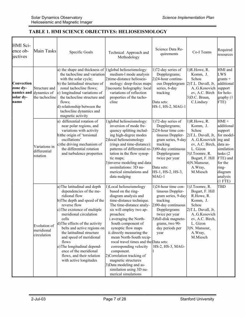
TABLE 1. HMI SCIENCE OBJECTIVES: HELIOSEISMOLOGY

HMI Sci-ence ob-jectives

Main Tasks Specific Goals

Technical Approach and Methodology

Science Data Re-quirements Co-I Teams Required

resources

Structure and dynamics of the tachocline

a) the shape and thickness of the tachocline and variation with the solar cycle;

b) the latitudinal structure of zonal tachocline flows;

c) longitudinal variations of the tachocline structure and flows;

d) relationship between the tachocline dynamics and magnetic activity

1) global helioseismology: medium-l mode analysis

2) time-distance helioseis-mology: deep-focus maps

3) acoustic holography: local variations of reflection properties of the tacho-cline

1) 72-day series of Dopplergrams;

2) 24-hour continu-ous Dopplergram series, 6-day tracking

Data sets: HS-1, HS-2, MAG-1

1) R.Howe, R. Komm, J. Schou

2) T.L. Duvall, Jr, A..G.Kosovichev, A.C. Birch

3) D.C. Braun, C.Lindsey

HMI and LWS grants + additional support for holography (1 FTE)

Variations in differential rotation

a) differential rotation of near polar regions, and variations with activity

b) the origin of ‘torsional oscillations’

c) the driving mechanism of the differential rotation and turbulence properties

1) global helioseismology: inversion of mode fre-quency splitting includ-ing high-degree modes

2) local helioseismology (rings and time-distance): patterns of differential ro-tation in the flow synop-tic maps;

3) inverse modeling and data assimilations: 3D nu-merical simulations and data nudging

1) 72-day series of Dopplergrams;

2) 24-hour time con-tinuous Doppler-gram series, 9-day tracking

3) 90-day continuous Dopplergrams twice per year

Data sets: HS-1, HS-2, HS-3, MAG-1

1) R.Howe, R. Komm, J. Schou

2) T.L. Duvall, Jr, A..G.Kosovichev, A.C. Birch, L. Gizon

3) J.Toomre, R. Bogart, F. Hill

4) N.Mansour, A.Wray, M.Miesch

HMI + additional support for model-ing and data as-similation tasks (2 FTE) and for the ring-diagram analysis (1 FTE)

Convection zone dy-namics and solar dy-namo

Evolution of meridional circulation

a) The latitudinal and depth dependencies of the me-ridional flow

b) The depth and speed of the reverse flow

c) The existence of multiple meridional circulation cells

d) The effects of the activity belts and active regions on the latitudinal structure and speed of meridional flows

e) The longitudinal depend-ence of the meridional flows, and their relation with active longitudes

1) Local helioseismology based on the ring-diagram analysis and time-distance technique. The time-distance analy-sis will employ two ap-proaches: i. averaging the North-South component of synoptic flow maps

ii. directly measuring the mean North-South recip-rocal travel times and the corresponding velocity component.

2) Correlation tracking of magnetic structures

3) Data modeling and as-similation using 3D nu-merical simulations

1) 24-hour time con-tinuous Doppler-gram series, 9-day tracking


3) full-disk magneto-grams, two 90-day periods per year


1) J.Toomre, R. Bogart, F. Hill R.Howe, R. Komm, J. Schou


3) N. Mansour, A.Wray, M.Miesch

TBD




Dynamics in the near sur-face shear layer

a) Mean stratification and thermodynamic properties, testing the equation of state

b) Structure and dynamics of supergranulation, the depth of the reverse flow, mass, energy and momen-tum transport

c) Variations of the subsur-face shear flow with lati-tude and time

d) Distribution of kinetic helicity and relation to large-scale magnetic pat-terns

e) Excitation and damping of p- and f-modes, waves-turbulence interaction

f) Understanding convective energy transport and role in irradiance

1) High-degree global helio-seismology: inversion of frequencies and fre-quency splitting of p- and f-modes of l=200-1000 to infer the subphotospheric rotation rate, sound-speed asphericity, and thermo-dynamic properties (adiabatic exponent and other properties of the equation of state;

2) Local helioseismology: synoptic flow and sound-speed maps

3) F-mode helioseismology (global and local)

4) Correlation analysis be-tween flows and mag-netic fields

5) Numerical simulations and data assimilation


2) full-disk magneto-grams, two 90-day periods per year

Data sets: HS-3, MAG-1

1) E. Rhodes, J. Reiter



4) N. Mansour, A.Wray, M.Miesch

Support for Johann Reiter + TBD

Origin and evolution of sunspots, active re-gions and complexes of activity

Formation and deep structure of magnetic complexes of activity

a) Relationship between large-scale flow patterns and magnetic flux emer-gence;

b) Impulses of solar activity and large-scale dynamics;

c) Search for thermal shad-ows in the interior

1) Deep-focus synoptic flow and sound-speed maps from time-distance helio-seismology and acoustic holography

2) Analysis of near-surface flow and sound-speed maps

3) Correlation analysis of the helioseismic and mag-netic data

1) 24-hour time continuous Dop-plergram series, 9-day tracking

2) 120-day continu-ous Dopplergrams, one period per year

3) full-disk mag-netograms, two 90-day periods per year


1) T.L. Duvall, Jr, A..G.Kosovichev, A.C. Birch


TBD




Active region source and evolution

a) Tracking the lifecycle of selected active regions (emergence, evolution, decay)

b) Detection of emerging flux in the interior

c) Relationship between large-scale flow patterns and stability of active re-gions

d) Search for signatures of disconnection of magnetic flux from deep interior structures

e) The depth is the circulation flow around active regions

f) How active regions affect the structure and speed of meridional flows

g) The role of magnetic re-connections in the corona for the evolution of active regions

h) Submergence of magnetic flux

1) Local helioseismology of selected active regions with 8-hour resolution (deep and surface focusing schemes)

2) Time-distance analysis of emerging active regions for 2-hour intervals

3) Relationship between the synoptic flow patterns and local flows around active regions

4) Correlation between the internal flows and sound-speed perturbations and photospheric field

5) Connectivity of active regions in the corona and their evolution

1) 24-hour time continuous Dop-plergram series, 9-day tracking

2) 12-day continu-ous Dopplergrams, 20 periods per year

3) full-disk mag-netograms, twenty 12-day periods per year

4) coronal EUV images


1) T.L. Duvall, Jr, A..G.Kosovichev, J. Zhao, S.Couvidat

2) J.Toomre, R. Bogart, F. Hill R.Howe, R. Komm, J.

3) C.Lindsey, D.C. Braun

TBD

Magnetic flux concentration in sunspots

a) Relationship between the flow dynamics and flux concentration in sunspots

b) The relation between the Evershed effect and deep flow pattern

c) Determination of the rela-tive role of temperature and magnetic perturba-tions in the sound-speed images

d) Relation between the inter-nal vortex flows, magnetic twists of sunspots and coronal activity

e) Connectivity between sunspots in active regions

f) Prediction of lifetime of sunspots by observing the internal circulation

1) Local helioseismology of selected active regions with 8-hour resolution (deep and surface focus-ing schemes)

2) Time-distance analysis of rapidly growing sunspots for 2-hour intervals

3) Relationship local flows around sunspots, mag-netic field, and EUV loop structures

4) Numerical modeling and data assimilation

1) 24-hour time con-tinuous Doppler-gram series, 9-day tracking12-day continuous Dop-plergrams, 20 pe-riods per year

2) full-disk magneto-grams, twenty 12-day periods per year

3) coronal EUV images

Data sets: HS-2, HS-5, MAG-

3

1) T.L. Duvall, Jr, A..G.Kosovichev, J. Zhao, S.Couvidat

2) J.Toomre, R. Bogart, F. Hill R.Howe, R. Komm, J.

3) C.Lindsey, D.C. Braun

4) N. Mansour, A.Wray,

TBD




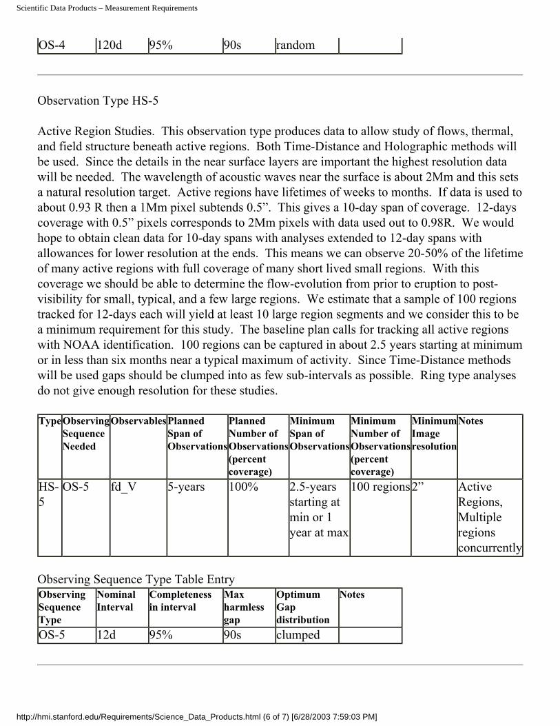
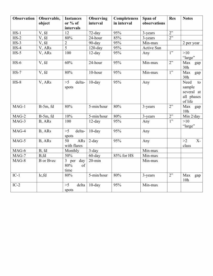
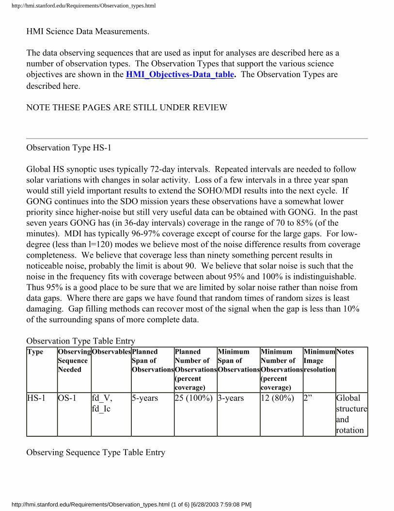
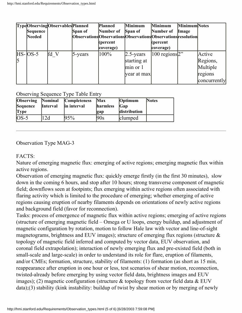
A new description of the Observation Types (e.g. HS-1) is being developed and is in this directory as Observation_types.doc and Observation_types.html.

Observa-tion

Observ-able, object

Instances or % of intervals

Observing interval

Com-plete-ness in interval

Span of observa-tions

Res Notes

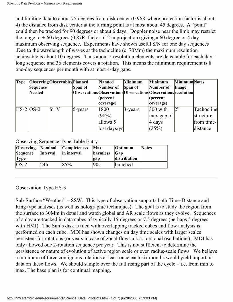
HS-1 V, fd 12 72-day 95% 3-years 2” HS-2 V, fd 80% 24-hour 85% 3-years 2” HS-3 V, fd 2 90-day 95% Min-max 2 per year HS-4 V, ARs 5 120-day 95% Active

Sun

HS-5 V, ARs 100 12-day 95% Any 1” >10 “large” HS-6 V, fd 60% 24-hour 95% Min-max 2” Max gap 30h HS-7 V, fd 80% 10-hour 95% Min-max 1” Max gap 30h HS-8 V, ARs >5 delta-

spots 10-day 95% Any Need to sample

several at all phases of life

MAG-1 B-5m, fd 80% 5-min/hour 80% 3-years 2” Max gap 10h MAG-2 B-5m, fd 10% 5-min/hour 80% 3-years 2” Min 2/day MAG-3 B, ARs 100 12-day 95% Any 1” >10 “large” MAG-4 B, ARs >5 delta-

spots 10-day 95% Any

MAG-5 B, ARs 50 ARs with flares

2-day 95% Any >2 X-class

MAG-6 B, fd Monthly 3-day Min-max MAG-7 B,fd 50% 60-day 85% for

HS Min-max

MAG-8 B or Bvec

3 per day 80% of time

20-min Min-max

IC-1 Ic,fd 80% 5-min/hour 80% 3-years 2” Max gap 10h IC-2 >5 delta

spots 10-day 95% Min-max


http://hmi.stanford.edu/Requirements/Observation_types.doc



Objective 1. Convection-zone dynamics and the solar dynamo

Fluid motions inside the Sun generate the solar magnetic field. Complex interactions between turbulent convection, rotation, large-scale flows and magnetic field produce regular patterns of solar activity changing quasi-periodically with the solar cycle. How are variations in the solar cycle related to the internal flows and surface magnetic field? How is the differential rotation pro-duced? What is the structure of the meridional flow and how does it vary? What role do the tor-sional oscillation pattern and the variations of the rotation rate in the tachocline play in the solar dynamo?

These issues are usually studied only in zonal averages by global helioseismology but the Sun is longitudinally structured. Local helioseismology has revealed the presence of large-scale horizon-tal flows within the near-surface layers of the solar convection zone. These flows possess intricate patterns that change from one day to the next, accompanied by more gradually evolving patterns such as banded zonal flows and meridional circulation cells. These flow structures have been de-scribed as Solar Subsurface Weather (SSW). Synoptic maps of these weather-like flow structures suggest that solar magnetism strongly modulates flow speeds and directions. Active regions tend to emerge in the stronger shear latitudes. The connections between SSW and active region devel-opment are presently unknown.

Main tasks:

1A. Structure and dynamics of the tachocline

1B. Variations in differential rotation

1C. Evolution of meridional circulation

1D. Dynamics in the near-surface shear layer

2.2.1.A Task 1A. Structure and dynamics of the tachocline

Major goals and significance

Direct observation of the deep roots of the solar activity in the tachocline located at the base of the solar convection zone, at 0.7 R, is of primary importance for understanding the long-term vari-ability of the Sun. Recent results from MDI and GONG have revealed intriguing 1.3-year quasi-periodic variations of the rotation rate in the tachocline, which may be a key to understanding the solar dynamo. An important task of HMI is to confirm these findings and determine the relation-ship between the dynamics of the tachocline and magnetic activity. The major specific tasks are to determine:

a) the shape and thickness of the tachocline zone and its variations with solar cycle;

b) the latitudinal dependence of the evolving zonal flows at the base of the convection zone;

c) longitudinal variations of the structure and flows at the base of the convection zone;

d) the relationship between the tachocline dynamics and magnetic activity.

These studies will provide information about the main processes of the Sun’s magnetic activity cycle, and important constraints for theories of the solar dynamo.




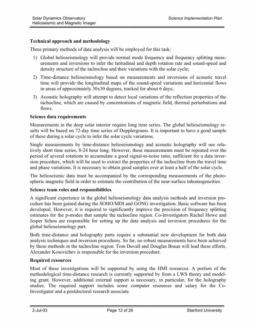
Technical approach and methodology Three primary methods of data analysis will be employed for this task:

1) Global helioseismology will provide normal mode frequency and frequency splitting meas-urements and inversions to infer the latitudinal and depth rotation rate and sound-speed and density structure of the tachocline and their variations with the solar cycle;

2) Time-distance helioseismology based on measurements and inversions of acoustic travel time will provide the longitudinal maps of the sound-speed variations and horizontal flows in areas of approximately 30x30 degrees, tracked for about 6 days;

3) Acoustic holography will attempt to detect local variations of the reflection properties of the tachocline, which are caused by concentrations of magnetic field, thermal perturbations and flows.

Science data requirements Measurements in the deep solar interior require long time series. The global helioseismology re-sults will be based on 72-day time series of Dopplergrams. It is important to have a good sample of these during a solar cycle to infer the solar cycle variations.

Single measurements by time-distance helioseismology and acoustic holography will use rela-tively short time series, 8-24 hour long. However, these measurements must be repeated over the period of several rotations to accumulate a good signal-to-noise ratio, sufficient for a data inver-sion procedure, which will be used to extract the properties of the tachocline from the travel time and phase variations. It is necessary to obtain good samples over at least a half of the solar cycle.

The helioseismic data must be accompanied by the corresponding measurements of the photo-spheric magnetic field in order to estimate the contribution of the near-surface inhomogeneities.

Science team roles and responsibilities A significant experience in the global helioseismology data analysis methods and inversion pro-cedure has been gained during the SOHO/MDI and GONG investigation. Basic software has been developed. However, it is required to significantly improve the precision of frequency splitting estimates for the p-modes that sample the tachocline region. Co-Investigators Rachel Howe and Jesper Schou are responsible for setting up the data analysis and inversion procedures for the global helioseismology part.

Both time-distance and holography parts require a substantial new development for both data analysis techniques and inversion procedures. So far, no robust measurements have been achieved by these methods in the tachocline region. Tom Duvall and Douglas Braun will lead these efforts. Alexander Kosovichev is responsible for the inversion procedure.

Required resources Most of these investigations will be supported by using the HMI resources. A portion of the methodological time-distance research is currently supported by from a LWS theory and model-ing grant. However, additional external support is necessary, in particular, for the holography studies. The required support includes some computer resources and salary for the Co-Investigator and a postdoctoral research associate.




2.2.1.B Task 1B. Variations in differential rotation.

Major goals and significance Differential rotation is a crucial component of the solar cycle and is believed to generate the global scale toroidal magnetic field expressed in active regions. HMI will use global and local helioseismic techniques to measure the solar differential rotation, investigate relations between variations of rotation and magnetic fields, longitudinal structure of zonal flows (‘torsional oscilla-tions’), relations between the torsional pattern and active regions, measure the subsurface shear and its variations with solar activity, and the origin of the ‘extended’ solar cycle. The major goals of this investigation are to determine:

a) differential rotation in the polar regions, short- and long-term variations of the rotation rate, and their relations to the polar magnetic field and the ‘extended solar cycle’ phenomenon;

b) the origin of the ‘torsional oscillations’, and their role in the solar cycle;

c) the driving mechanism of the differential rotation and related properties of solar turbulent convection.

Technical approach and methodology For solving these problems it is essential to combine the results of the traditional inversions of rotational frequency splitting with inferences of local helioseismology and numerical models. More specifically, the technical approach is based on the following three methods:

1) inversion of normal mode frequency splitting; this dataset will include high-degree modes and also more accurate measurements of tesseral modes of low angular order m, which probe the near-polar regions;

2) investigation of patterns of differential rotation and torsional oscillations using synoptic maps of horizontal flows and sound-speed variations inferred by local helioseismology;

3) inverse modeling and data assimilation based three-dimensional numerical simulations of turbulent solar convection; these will include nudging, adaptive Kalman-type filtering and other techniques to obtain information about properties of solar turbulence and thermal and magnetic effects that lead to the observed differential rotation law and torsional oscillations.

Science data requirements The primary data set for the global helioseismology inversions is 72-day time series of full-disk Dopplergrams. Because of the better coverage of the Sun’s polar regions the HMI will provide more accurate estimates of frequencies and frequency splitting of low-m modes, and thus will extend the zone of helioseismic inferences for the differential rotation and asphericity closer to the Sun’s poles. Tracking the changes with the solar cycle in the near polar regions is extremely im-portant for studying the mechanisms of the polar magnetic field reversals and the solar dynamo. Therefore, these measurements should continue for at least a half of the solar cycle.

The synoptic maps of subsurface flows and sound-speed structures will be made by two different techniques: time-distance helioseismology and ring-diagram analysis. The synoptic map method-ology that is currently being developed for analysis of MDI full-disk Dopplergrams will be




adopted for HMI. The time-distance procedure uses 512-min series of full-disk MDI Doppler-grams covering a central meridian zone 30o wide and from -54o to +54o in latitude. The horizon-tal resolution is 0.24o; the vertical resolution varies from 1.5 to 3 Mm in the 0-20 Mm depth range. The HMI will allow extending the latitudinal coverage and improving the spatial resolu-tion. The precise characteristics of the HMI subphotospheric synoptic maps will be determined when the HMI become available. The ring-diagram synoptic maps are obtained by measuring local frequency shifts in 15x15-degree areas on 7.5-degree grid, using 1-day time series. The depth resolution is similar to the time-distance technique. These two approaches are based on dif-ferent properties of solar oscillations and, thus, provide independent estimates for solar rotation. Typically, the correlation coefficient between the time-distance and ring-diagram maps is 0.7-0.8.

Data assimilation and inverse modeling is a new approach for high-level data analysis. It employs numerical models for inferring physical properties of the solar dynamics, such as turbulent trans-port coefficients and Reynolds stress, from helioseismic inversion results. One of the methods which is being investigated is nudging, a method of dynamical relaxation. In nudging, the nu-merical models of the differential rotation are gently adjusted towards to the observations by add-ing a forcing function, in such a way that the difference between the observed and numerical re-sults is minimized. This will allow us to track the corresponding changes in the model and made conclusions about the physical processes. This approach requires the inversion results for differ-ential rotation and meridional circulation and 3D numerical simulations of solar convection in spherical geometry.

Science team roles and responsibilities

Co-Investigators, Rachel Howe and Jesper Schou, have taken the responsibility for the global helioseismology results. Tom Duvall leads the efforts for obtaining the synoptic flow and sound-speed maps by the time-distance technique. Juri Toomre, Richard Bogart, and Frank Hill coordi-nate the development of the ring-diagram method and analysis. Nagi Mansour have taken the lead n the data assimilation task.

Required resources The production of the synoptic flow and sound-speed maps is a part of the HMI data processing, as well as the global mode analysis. Additional resources are required for the science analysis of these data, studying correlations with magnetic field and irradiance measurements and models, and numerical modeling and data assimilation (at least, 2 postdoctoral associates for these tasks). Also, an external support is required for the production ring-diagram synoptic maps and their analysis (1 research associate).

2.2.1.C Task 1C. Evolution of meridional circulation.

Major goals and significance Precise knowledge of the meridional circulation is crucial for understanding the long-term vari-ability of the Sun. Helioseismology has found evidence for poleward flow variation with the solar cycle. To understand the global dynamics we must follow the evolution of the flow. HMI will generate continuous data for detailed, 3-D maps of the evolving patterns of meridional circulation providing information about how flows transport and interact with magnetic fields during the so-lar cycle.




The key goals are to determine:

a) the latitudinal and depth dependences of the mean meridional flow;

b) the depth and speed of the reverse flow;

c) the existence of multiple meridional circulation cells;

d) the effects of the activity belts and active regions on the latitudinal structure and speed of meridional flows;

e) the longitudinal dependence of the meridional flows, and their relation with active longi-tudes.

Technical approach and methodology The main tools for the investigation of meridional circulation are:

1)local helioseismology based on the ring-diagram analysis and the time-distance technique; the time-distance results will be obtained by using two different approaches:

a. averaging the North-South component of velocity of the synoptic flow maps;

b. directly measuring averaged travel times of acoustic waves propagating in the North-South direction;

2)correlation tracking of magnetic structures will provide a very important complementary in-formation about the magnetic flux transport in the photosphere, and potential structure and strength of meridional flows in deeper layers;

3)data modeling and assimilation by using 3D numerical models; these models typically show multiple cells, and the challenge is to match the observed flow, and determine the corre-sponding properties of solar turbulence (transport coefficients, Reynolds stress etc).

Science data requirements The local helioseismology require 24-hour continuous series of Dopplergrams during at least 6 months each year (e.g. every other month). MDI results have demonstrated that 2-3 months per is insufficient for following the evolution of the meridional flows.

Science team roles and responsibilities The local helioseismology ring-diagram effort is led by Juri Toomre and Frank Hill. The members of their teams are Deborah Haber, Brad Hindman, Rick Bogart, Rachel Howe, and Rudi Komm. The time-distance measurements are coordinated by Tom Duvall; the data inversions are carried out by Alexander Kosovichev and their colleagues. The magnetic field tracking task is not yet assigned. A similar study has been done by Nadege Meuner using the MDI data.

Required resources The ring-diagram and magnetic field tasks will require an external support.




2.2.1.D Task 1D. Dynamics in the near-surface shear layer.

Major goals and significance Helioseismology has revealed that the most significant changes with the solar cycle occur in the near-surface shear layer. However, the physics of these variations and their role in the irradiance variations are still unknown. HMI will characterize the properties of the near-surface shear layer, assay the interaction between surface magnetism and evolving flow patterns, and trace the modi-fications in the structure and dynamics as the solar cycle advances. It will assess the statistical properties of convective turbulence over the solar cycle, including the kinetic helicity and its rela-tion the magnetic helicity – two most intrinsic characteristics of the dynamo action. The physics of the near surface turbulent layer is very rich. Here we identify only some initial goals of this investigation task, which are to determine:

a) mean stratification and thermodynamic properties, testing the equation of state of the solar plasma;

b) structure and dynamics of supergranulation, the depth of the reverse flow, mass and energy balance, the interaction with the rotational shear flow;

c) variations of the subsurface shear flow with latitude and time;

d) distribution of kinetic helicity, and its relation to large-scale magnetic patterns of the photo-sphere;

e) excitation and damping mechanism of solar p- and f-modes; interaction between waves and turbulence;

f) understanding of convective energy transport: most solar energy is transported to the solar sur-face by convection. Properties of the turbulent convection and its efficiency of transporting the energy flux may vary with both time and location. Therefore, it is extremely important to study the energetics of solar convection, and to establish the characteristics that affect the energy transport. Links between convection and the cycle can be manifested in the internal variations in wave speed, in the distribution of surface brightness, and in the shape of the solar limb. HMI will monitor these properties for an extended period of time, thus providing new insight in how the energy flows inside the Sun and affects solar irradiance.

Comprehensive multi-scale helioseismology and vector magnetic field data combined with the AIA observations of the solar corona will offer an unprecedented opportunity to solve the prob-lem of the origin of solar activity, which puzzled people for almost four centuries since Galileo’s discovery of sunspots, and is central to the LWS program.

Technical approach and methodology The near surface shear layer is accessible by all helioseismology techniques, both global and lo-cal, and this allows us to cross-check the measurements, and obtain robust inferences of various physical properties of this layer. In particular, this methodology includes

1)deriving latitudinal and depth dependencies of the rotation rate and sound-speed variations by inversion of global modes frequencies and frequency splitting;

2)obtaining synoptic flow maps of various resolution by the local ring-diagram and time-distance methods, and then averaging these maps over longitude provides an independent estimate of the rotation rate and global latitudinal sound speed variations;




3)using the surface gravity waves (f-modes) for both global and global diagnostics of subpho-tospheric and photospheric motions;

4)studying correlations between subphotospheric flow patterns and characteristics of magnetic activity such as magnetic and kinetic helicity;

5)comparing the observed properties of supergranulation and larger scale flows with results of numerical simulations.

Science data requirements The global helioseismology investigations will employ the measurements of frequencies and fre-quency splitting for high-degree (l=200 – 2000) modes. The technique for these is being devel-oped by Ed Rhodes and Johann Reiter. The current application this technique to the MDI data shows that it is extremely important to take into account the image distortions (these should be known to a high precision), as well as the mode interaction due large-scale inhomogeneities, like the differential rotation.

The local helioseismology require 24-hour continuous series of Dopplergrams during at least 6 months each year (e.g. every other month). MDI results have demonstrated that 2-3 months per is insufficient for following the evolution of the shear flows. The supergranulation studies by the time-distance technique require continuous 10-day chunks of Dopplergrams for tracking the evo-lution of supergranules as they move across the solar disk.

Science team roles and responsibilities

The local helioseismology ring-diagram effort is led by Juri Toomre and Frank Hill. The members of their teams are Deborah Haber, Brad Hindman, Rick Bogart, Rachel Howe, and Rudi Komm. The time-distance measurements are coordinated by Tom Duvall; the data inversions are carried out by Alexander Kosovichev and their colleagues.

Required resources TBD

2.2.2 Objective 2. Origin and evolution of sunspots, active regions and complexes of activ-ity

Observations show that magnetic flux on the Sun does not appear randomly. Once an active re-gion emerges, there is a high probability that additional eruptions of flux will occur in the neighborhood, or even in the same region (activity nests, active longitudes). How is magnetic flux synthesized, concentrated, and transported to the solar surface where it emerges in the form of evolving active regions? To what extent are the appearances of active regions predictable? What roles do local flows play in active region evolution?

HMI will answer these questions by providing tracked sound-speed and flow maps for individual active regions and complexes under the visible surface of the Sun combined with surface mag-netograms. Current thinking suggests that the flux emerging in active regions originates in the tachocline. Flux is somehow pulled from the depths in the form of loops that rise through the convection zone and emerge through the surface. Phenomenological flux transport models show that the photospheric distribution of flux requires no long-term connection to flux below the sur-face. Rather, field motions are described by the observed poleward flows, differential rotation,




and surface diffusion acting on emerged flux of active regions. Does the active region magnetic flux really disconnect from the deeper flux ropes after emergence?

Main tasks: 2A. Formation and deep structure of magnetic complexes of activity

2B. Active region source and evolution

2C. Magnetic flux concentration in sunspots

2D. Sources and mechanisms of solar irradiance variations

2.2.2.A Task 2A. Formation and deep structure of magnetic complexes of activity.

Major goals and significance HMI will explore the nature of long-lived complexes of solar activity (‘active or preferred longi-tudes’), the principal sources of solar disturbances. The phenomenon of ‘active longitudes’ has been one of the main puzzles of solar activity for many decades. Active longitudes may continue from one cycle to the next, and may be related to variations of solar activity on the scale of 1-2 years and short-term ‘impulses’ of activity. HMI will probe beneath these features to 0.7R, the bottom of the convection zone, to search for correlated flow or thermal structures

2.2.2.B Task 2B. Active region source and evolution.

By using acoustic tomography we can image magnetic flux emergence and the disconnection that may occur. Vector magnetograms give evidence whether flux leaves the surface predominantly as ‘bubbles’, or whether it is principally the outcome of local annihilation of fields of opposing po-larity. With a combination of helioseismic probing and vector field measurements HMI will pro-vide new insight into active region flux emergence and removal.

2.2.2.C Task 2C. Magnetic flux concentration in sunspots.

Formation of sunspots is one of the long-standing problems of solar physics. Recent observations from MDI have revealed complicated flow patterns beneath sunspots (Fig. C.5) and indicated that the highly concentrated magnetic flux in spots is accompanied by converging mass flows in the upper 3-4 Mm beneath the surface (Foldout 1.I). The evolution of these flows is not presently known. HMI observations will allow investigating relations between the flow dynamics and flux concentration in spots, the flows in the deeper layers, below 4 Mm, providing detailed maps of the subsurface flows combined with surface fields and brightness for 9 days during the passage of sunspots on the solar disk.

2.2.2.D Task 2D. Sources and mechanisms of solar irradiance variations. Magnetic features - sunspots, active regions, and network - that alter the temperature and compo-sition of the solar atmosphere are primary sources of solar irradiance variability. How exactly do these feature cause the irradiance variations? HMI together with the other SDO instruments AIA




and EIS will study physical processes that govern these variations and the relation between the interior processes, properties of magnetic field regions and irradiance variations, particularly, the UV and EUV components that have a direct and significant effect on Earth’s atmosphere.

2.2.3 Objective 3. Sources and drivers of solar activity and disturbances

It is commonly believed that the principal driver of solar disturbances is stressed magnetic field. The stresses are released in the solar corona producing flares and coronal mass ejections (CME). The source of these stresses is believed to be in the solar interior. Flares usually occur in the areas where magnetic configuration is complicated, with strong shears, high gradients, long and curved neutral lines, etc. This implies that the trigger mechanisms of flares strongly depend on critical properties of magnetic field that lead eventually to MHD instabilities. But what kind of instability actually works, and under what conditions it is triggered are unknown. Beside some theoretical ideas and models, there is no knowledge of how magnetic field is stressed or twisted inside the Sun or just what the triggering process is.

Main tasks: 4A. Origin and dynamics of magnetic sheared structures and delta-type sunspots

4B. Magnetic configuration and mechanisms of solar flares

4C. Emergence of magnetic flux and solar transient events

4D. Evolution of small-scale structures and magnetic carpet

2.2.3.A Task 3A. Origin and dynamics of magnetic sheared structures and δ-type sunspots. Recent observations from MDI discovered complicated patterns of shearing and twisting flows beneath rapidly evolving active regions. Understanding the evolution of these flows and their coupling to activity requires continuous high-resolution observations. Particularly interesting tar-gets of this investigation are δ-type sunspots. These spots contain two umbra of opposite magnetic polarities within a common penumbra and are the source of the most powerful flares and CMEs. The δ-type sunspot regions are thought to emerge magnetic flux into the solar atmosphere in a highly twisted state. It is important to determine what processes beneath the surface lead to devel-opment of these spots and make them active producing flares and CME.

2.2.3.B Task 3B. Magnetic configuration and mechanisms of solar flares and CME. HMI vector magnetic field measurements can be used to infer the field topology configuration and the vertical electric current, both of which are essential to understand the flare process. Ob-servations are required that can show continuous changes of magnetic field and electric current before flares with sufficient spatial resolution to show changes of the field strength and topology before and after flares. HMI will provide these unique measurements of the vector magnetic field over the whole solar disk with reasonable accuracy and at high cadence.

2.2.3.C Task 3C. Emergence of magnetic flux and solar transient events.

Emergence of magnetic flux is closely related to solar transient events. Quick emergence of mag-netic flux within active regions is found to be associated with flares. Emerging magnetic flux re-gions near filaments lead to eruption of filaments. CMEs are also found to accompany emerging flux regions. However, emergence of isolated active regions often does not cause any eruptive




events. This implies that magnetic flux emerging into the atmosphere interacts with the pre-existing magnetic field leading to loss of magnetic field stability. Electric current systems and magnetic topology between the newly emerging magnetic flux and the pre-existed field are the keys to understand why emerging magnetic flux causes solar transient events. Vector polarimetry provided by HMI is essential for quantitative studies of magnetic topology changes of both pre-existing field and emerging flux regions.

2.2.3.D Task 3D. Evolution of small-scale structures and magnetic carpet. The quiet Sun is covered with small regions of mixed polarity, termed ‘magnetic carpet’. These small-scale magnetic elements contribute to solar activity on short timescales. As these elements erupt through the photosphere they interact with each other and with larger magnetic structures such as those associated with active regions. They may provide triggers for eruptive events, and their constant interactions may be one of the sources of coronal heating. They may also contribute to irradiance variations in the form of enhanced network emission. HMI will make global scale observations of the small-scale magnetic element distribution, their interactions, and the resulting transformation of the large-scale field.

2.2.4 Objective 4. Links between the internal processes and dynamics of the corona and heliosphere

The highly structured solar atmosphere is dominantly governed by magnetic field generated in the solar interior. Magnetic fields and the consequent coronal structures occur on many spatial and temporal scales. Intrinsic connectivity between multi-scale patterns increases coronal structure complexity leading to variable phenomena. For example, CMEs are believed to be related to the global-scale magnetic field, but many CMEs, especially fast CMEs, have been found to be associ-ated with flares that are believed to be local phenomena. It is natural to link coronal structures and activity to internal processes and to link geoeffectiveness to solar coronal variability. However, it is a great challenge to provide a complete physical description to thoroughly explain the observed phenomena. Model-based reconstruction of 3-D magnetic structure is one way to calculate the field from observations. It has been shown that calculation from vector field data in active regions provides the best match to the observations. More realistic MHD coronal models based on HMI high-cadence vector-filed synoptic data as boundary conditions are also anticipated to revolution-ize our view of how the corona responds to evolving, non-potential active regions.

Main tasks:

4A. Complexity and energetics of the solar corona

4B. Large-scale coronal field estimates

4C. Coronal magnetic structure and solar wind

2.2.4.A Task 4A. Complexity and energetics of solar corona. Observations from SOHO and TRACE have shown a variety of complex structures and eruptive events in the solar corona. However, categorizing complex structures has not revealed the under-lying physics of the corona and coronal events. To make progress in understanding this very complex system, we need to extract the physics of the energization of the corona. Two mecha-nisms are proposed to generate stressed magnetic fields: photospheric shear motions and emerg-ing magnetic flux; and both may, in fact, be at work on the Sun. But which plays a dominant role




and how the energy injection is related to eruptive events is unknown. Methodologies are avail-able to estimate the magnetic energy and helicity and energy across the photosphere. The mag-netic helicity is an important characteristic of magnetic complexity; and its conservation intrinsi-cally links the generation, evolution and reconnections of the magnetic field. HMI will provide all the data necessary for estimating ejections of energy and helicity in active regions: the vector magnetic field and the velocity field (from helioseismology and correlation tracking). Observa-tions from AIA and WCI that show the consequent response and propagation of complexity in solar corona and heliosphere, will provide the data required to relate the build-up of helicity and energy with energetic coronal events such as CME’s.

2.2.4.B Task 4B. Large-scale coronal field estimates.

Models computed from line-of-sight photospheric magnetic maps have been used to reproduce coronal forms that show multi-scale closed field structures as well as the source of open field which starts from coronal holes but spreads to fill interplanetary space. Modeled coronal field demonstrates two types of closed field regions, helmet streamers that form the heliospheric cur-rent sheet and another one that is sandwiched between the like-polarity open field regions. There is evidence that most CMEs are associated with helmet streamers and with newly opened flux. HMI will provide magnetic coverage at a high cadence, and together with contemporaneous AIA, WCI and STEREO coronal images will enable the development of coronal field models and stud-ies of the relationship between pre-existing patterns, newly opening fields, long distance connec-tivity, and CMEs.

2.2.4.C Task 4C. Coronal magnetic structure and solar wind. MHD simulation and current-free coronal field modeling based on magnetograms are two ways to study solar wind properties and their relations with coronal magnetic field structure. These meth-ods have proven effective and promising, showing potential in applications of real-time space weather forecasting. It has been demonstrated that the modeling of solar wind can be significantly improved with increased cadence of the input magnetic data. By providing full disk vector field data at high cadence, HMI will enable these models to describe the distribution of the solar wind, coronal holes and open field regions, how magnetic fields in active regions connect with inter-planetary magnetic field lines, and how interactions of streams produce co-rotating interaction regions.

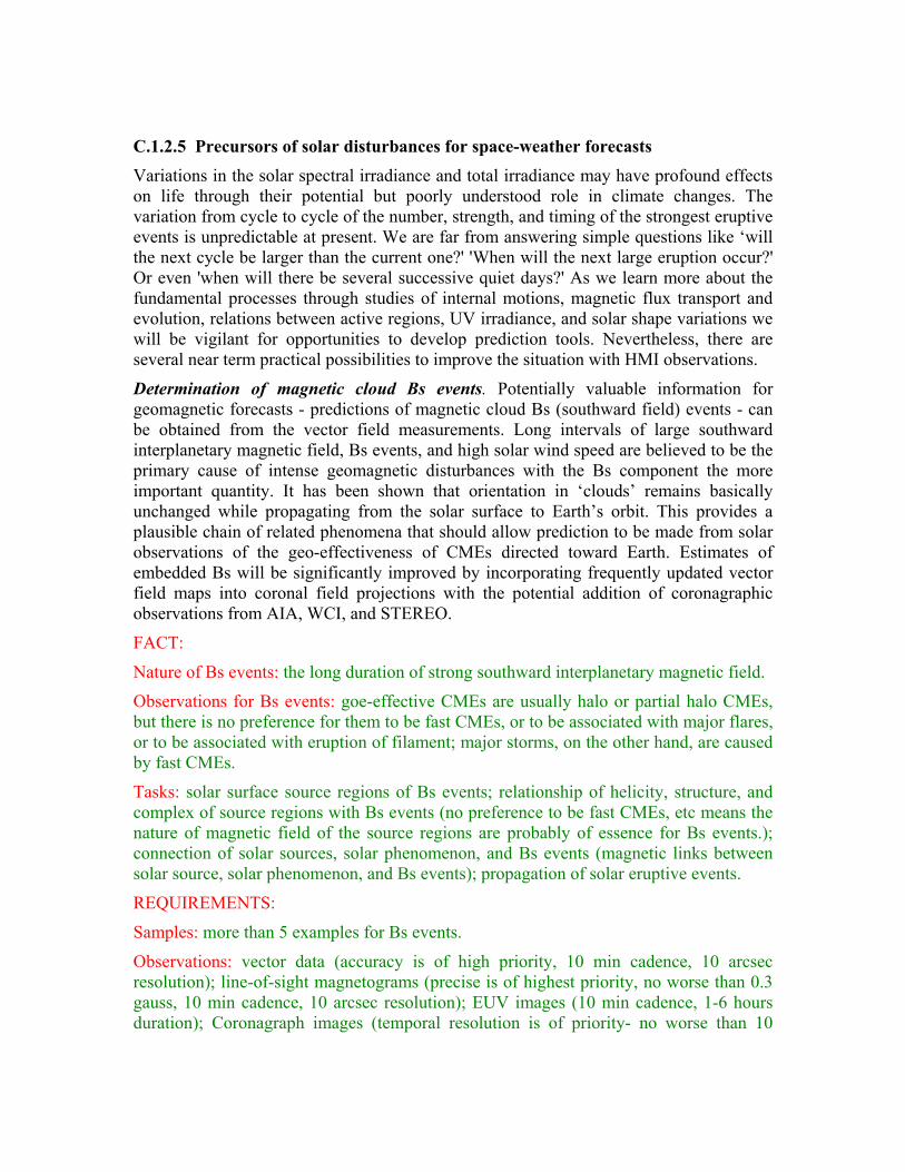
2.2.5 Objective 5. Precursors of solar disturbances for space-weather forecasts Variations in the solar spectral irradiance and luminosity may have profound effects on life through their potential but poorly understood role in climate changes. The variation from cycle to cycle of the number, strength, and timing of the strongest eruptive events is essentially not pres-ently predictable. We are far from answering simple questions like ‘will the next cycle be larger than the current one?’ Our understanding of the solar variations is fundamentally incomplete. To address the real-world questions we must solve this scientific problem. While developing correla-tive relations, detailed predictions must await a better understanding of the processes that govern the cycle. Meanwhile, there are several areas of investigation that can improve both our under-standing of the cycle as a process. As we learn more about the fundamental processes through studies of internal motions, magnetic flux transport and evolution, relations between active re-




gions, UV irradiance, and solar shape variations we will be vigilant for opportunities to develop prediction tools.

Main tasks:

5A. Far-side imaging and activity index

5B. Predicting emergence of active regions by helioseismic imaging

5C. Determination of magnetic cloud Bs events

2.2.5.A Task 5A. Far-side imaging and activity index. A procedure for solar far-side imaging was developed using data from MDI, and has led to the routine mapping of the Sun’s farside (http://soi.stanford.edu/data/farside/). Acoustic travel-time perturbations are correlated with strong magnetic fields, providing a view of active regions well before they become visible as they move onto the disk at the East limb. Synoptic images, which are now able to cover the entire far hemisphere of the Sun , will provide the ability to forecast the appearance of large active regions up to 2 weeks in advance and allow the detection of regions, which emerge just a few days before rotating into view.

2.2.5.B Task 5B. Predicting emergence of active regions by helioseismic imaging. Rising magnetic flux tubes in the solar convection zone are likely to render significant Doppler signatures, which would provide forewarning of their impending emergence. Helioseismic images of the base of the convection zone will employ a similar range of p-modes as those used to con-struct images of the far side, and will have comparable spatial resolution. An important goal is to detect and monitor seismic signatures of persistent or recurring solar activity near the tachocline. This will serve as a basis for long-term forecasts of solar geomagnetic disturbances.

2.2.5.C Task 5C. Determination of magnetic cloud Bs events. Extremely valuable information for geomagnetic forecasts - determination of magnetic cloud Bs events - will be obtained from the vector field measurements. Long intervals of large southward interplanetary magnetic field, Bs events, and high solar wind speed are believed to be the primary cause of intense geomagnetic disturbances with the Bs component the more important quantity. It has been shown that orientation in ‘clouds’ remains basically unchanged while propagating from the solar surface to Earth’s orbit. This provides a plausible chain of related phenomena that should allow prediction to be made from solar observations of the geoeffectiveness of CMEs di-rected toward Earth. Estimates of embedded Bs will be significantly improved by incorporating frequently updated vector field maps into coronal field projections with the potential addition of coronagraphic observations from AIA and STEREO.

3 Scientific Approach The investigation described above is a comprehensive broad based investigation into the sources and mechanisms of solar variability and its impact on the space environment. An investigation with this scope requires the dedicated efforts of a diverse team of researchers. The real constraint to the scientific return from SDO generally and HMI in particular is likely to be the limits to the support of people to pursue data analysis and theory development. The HMI investigation will


http://soi.stanford.edu/data/farside/



attempt to optimize the scientific return be actively enabling Guest Investigators, as well as the HMI science team by providing convenient access to high level data products and workshops as appropriate.

HMI data and results will be crucial for the success of the whole SDO mission providing neces-sary key data for the coronal and irradiance instruments, in particular, magnetic filed measure-ments, energetic and helicity characteristics of active regions, flow maps associated with develop-ing active processes. The goal is in cooperation with the coronal instruments, particularly, with AIA, SIE and WCI, to develop a system approach to develop knowledge and understanding the solar and heliospheric aspects of the Sun-Earth system that directly affect life and society.

Important cooperation will be developed with other space missions and ground-based observato-ries. In particular, HMI will take over from MDI to provide a missing key observation to support STEREO data interpretation. Because STEREO has no magnetographs it must rely on other ob-servatories for monitoring the solar magnetic field conditions during its target CME event studies. The spatial resolution and vector capability of HMI will provide the basis for modeling the corona and solar wind underlying STEREO CMEs, as well as indications of the causes of these tran-sients. HMI will also provide global context for Solar B vector measurements that are focused on specific active regions, and also information on coronal holes and solar wind stream structure used in the interpretation of L1 solar wind monitor data from spacecraft like ACE. In the area of helioseismology cooperation with the GONG+ project will play very important role for cross-checks of helioseismic inferences in the common range of spatial and temporal resolution.




4 Theoretical Support and Modeling The maximum scientific benefit from HMI can be obtained only with a specific theoretical pro-gram which includes numerical simulations of wave excitation and propagation in magnetized plasma, magnetoconvection, local and global dynamo processes, magnetic flux emergence, mag-netic structures and MHD processes in the solar corona. Theoretical models for inversion of heli-oseismic and magnetic data are also extremely important for HMI data analyses. The inversion algorithms needs to be sufficiently fast to provide the science data products which are required for studying precursors of solar disturbances, such as full-disk maps of subsurface flows, far-side images and vector magnetograms, in almost real time. As a part of this project we will operate a 3-D radiation MHD code that is being developed by HMI Co-Is at the NASA Ames Research Center. The member of our research team will actively participate in the coordinated SDO Guest Investigator and LWS Theory and Modeling Programs.




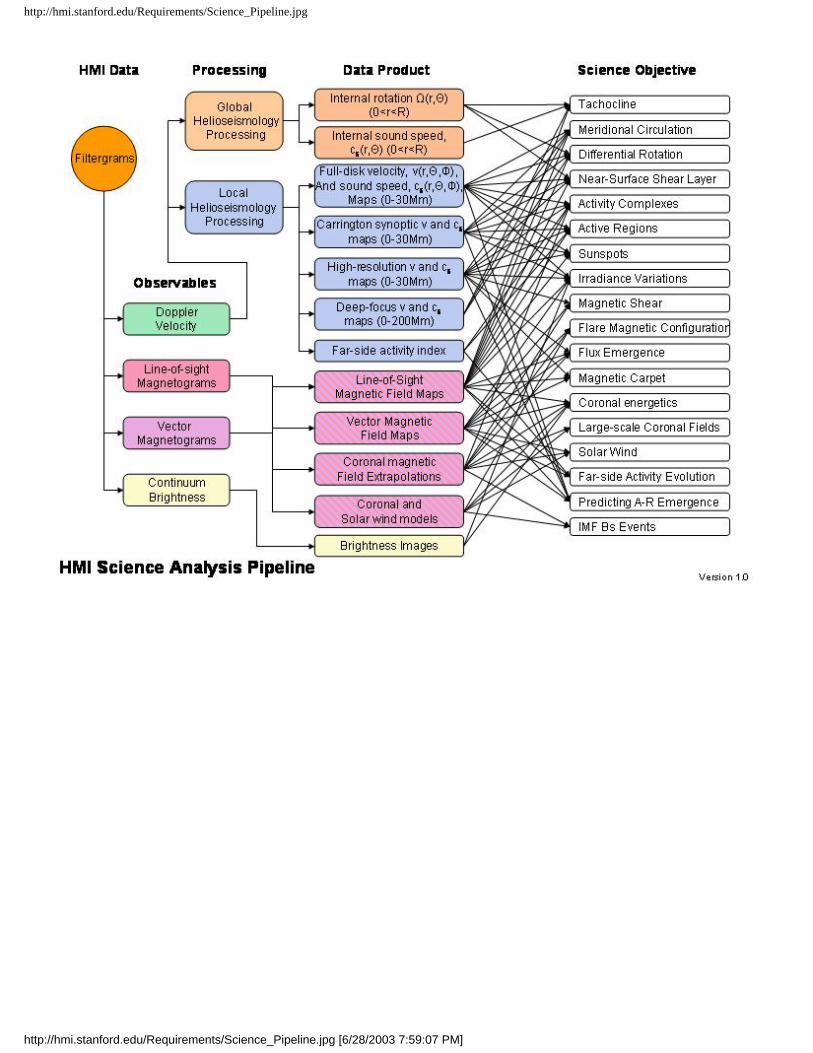
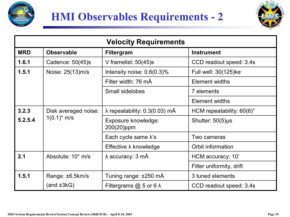
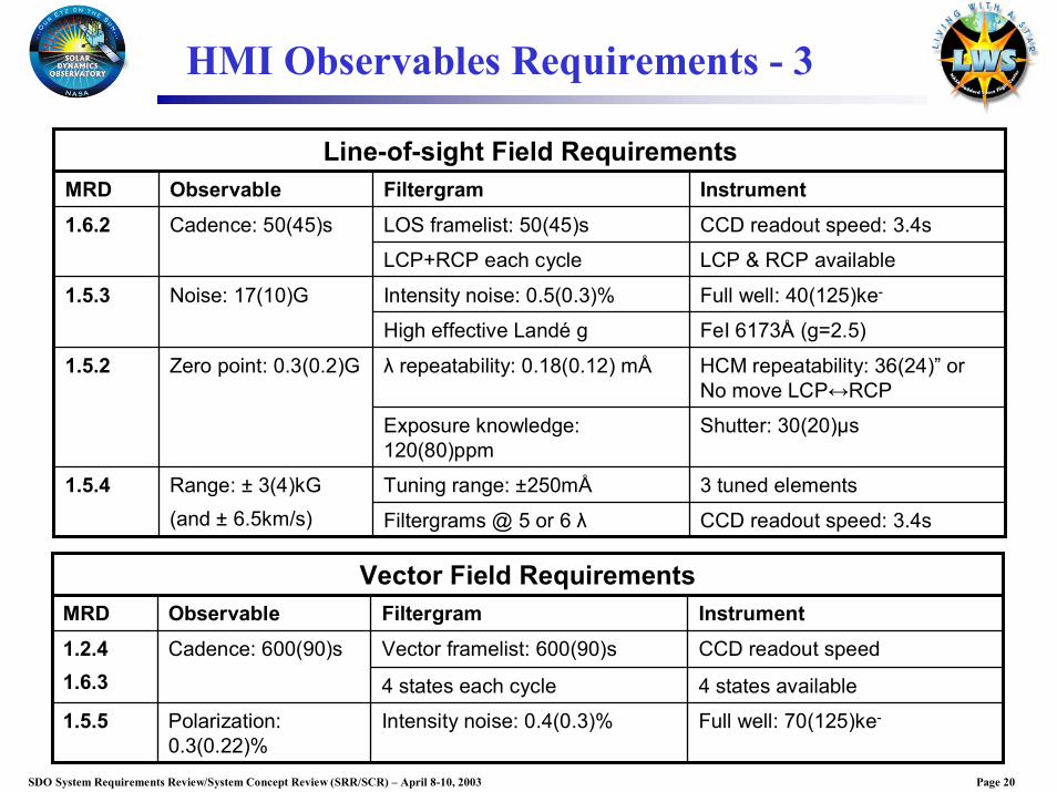
5 Scientific Operation Modes and Requirements The scientific operation modes and data products can be divided into four main areas: global heli-oseismology, local-area helioseismology, line-of-sight and vector magnetography and continuum intensity studies. The principal data flows and products are summarized in Table C.2.2. These four primary scientific analyses cover all main HMI objectives, and have the following character-istics:

Global Helioseismology: Diagnostics of global changes inside the Sun. The traditional normal-mode method will produce large-scale axisymmetrical distributions of sound speed, density, adia-batic exponent and flow velocities through the whole solar interior from the energy-generating core to the near-surface convective boundary layer. These diagnostics will be based on frequen-cies and frequency splitting of modes of angular degree up to 1000, obtained for several day in-tervals each month and up to l=300 for each 2-month interval. These will be used to produce a regular sequence of internal rotation and sound-speed inversions to allow observation of the ta-chocline and average near surface shear.

Local-Area Helioseismology: 3D imaging of the solar interior. New methods of local-area heli-oseismology, time-distance technique, ring-diagram analysis and acoustic holography represent powerful tools for investigating physical processes inside the Sun. These methods on measuring local properties of acoustic and surface gravity waves, such as travel times, frequency and phase shifts. They will provide images of internal structures and flows on various spatial and temporal scales and depth resolution. The targeted high-level regular data products include:

full-disk velocity and sound-speed maps of the upper convection zone (covering the top 30 Mm) obtained every 8 hours with the time-distance methods on a Carrington grid;

synoptic maps of mass flows and sound-speed perturbations in the upper convection zone for each Carrington rotation with a 2-degree resolution, from averages of full disk time-distance maps;

synoptic maps of horizontal flows in upper convection zone for each Carrington rotation with a 5 degree resolution from ring-diagram analyses.

higher-resolution maps zoomed on particular active regions, sunspots and other targets, ob-tained with 4-8-hour resolution for up to 9 days continuously, from the time-distance method;

deep-focus maps covering the whole convection zone depth, 0-200 Mm, with 10-15 degree resolution;

far-side images of the sound-speed perturbations associated with large active regions every 24 hours.

In addition, to this standard set new approaches such waveform tomography of small-scale struc-tures will be developed employed.

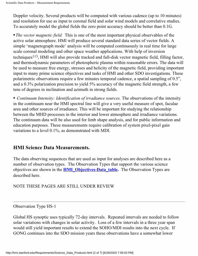
• Magnetography. Complete coverage of magnetic processes in the photosphere. The traditional line-of-sight component of the magnetic field is produced as a co-product with the Doppler veloc-ity observations used for helioseismology. This observable has proven to be very useful in track-ing magnetic field evolution at all time and size scales. Several products will be computed with various cadence and resolution for use as input to coronal field and solar wind models and cor-relative studies.




. The vector magnetic field is one of the most important physical observables of the active solar atmosphere. HMI will produce several standard data series of vector fields. A ‘magnetograph mode’ analysis will be computed routinely and continuously to provide boundary conditions for large scale coronal modeling. HMI, with help of robust inversion technique (Graham et al. 2002), will also provide AR tracked and full-disk on-request vector magnetic field, filling factor and the thermodynamic parameters of the photospheric plasma within reasonable errors. These data will be used to quantitatively measure the free energy of magnetic field, magnetic stresses and helicity, providing important input to many prime science objectives and tasks of HMI and other SDO investigations.

Continuum Intensity: Identification of irradiance sources. The observations of the intensity in the continuum near the HMI spectral line will give a very useful measure of spot, faculae area and other sources of irradiance. This will be important for studying the relationship between the MHD processes in the interior and lower atmosphere and irradiance variations. The continuum data will be also used for limb shape analysis, and for public information and education purposes.

• Real Time Products: Data for planning and prediction of space weather events. Some of data products will be made available for space weather investigations and forecasts in real time. The immediately available products includes: calibrated magnetograms, Doppler velocity and contin-uum intensity images. On the regular basis (daily or more often) we will provide full-disk maps of sound speed distribution and mass flows in the upper convection zone, and far-side activity index maps.




6 References

1. Hale, G.E., et al., 1919. The Magnetic Polarity of Sun-Spots. Astrophysical Journal, 49: p. 153.

2. Schrijver, C.J., et al., 1997. Sustaining the Quiet Photospheric Network: The Balance of Flux Emergence, Fragmentation, Merging, and Cancellation. Astrophysical Journal, 487: p. 424.

3. Title, A.M. and C.J. Schrijver. The Sun’s Magnetic Carpet. in ASP Conf. Ser. 154: Cool Stars, Stellar Systems, and the Sun. 1998.

4. Kosovichev, A.G., 1996. Helioseismic Constraints on the Gradient of Angular Velocity at the Base of the Solar Convection Zone. Astrophysical Journal, 469: p. L61.

5. Basu, S., 1997. Seismology of the base of the solar convection zone. Monthly Notices of the Royal Astronomical Society, 288: p. 572-584.

6. Charbonneau, P., et al., 1999. Helioseismic Constraints on the Structure of the Solar Ta-chocline. Astrophysical Journal, 527: p. 445-460.

7. Spiegel, E.A. and J.-P. Zahn, 1992. The solar tachocline. Astronomy and Astrophysics, 265: p. 106-114.

8. Canuto, V.M. and J. Christensen-Dalsgaard, 1998. Turbulence in Astrophysics: Stars. An-nual Review of Fluid Mechanics, 30: p. 167-198.

9. Durney, B.R., 2000. Meridional Motions and the Angular Momentum Balance in the Solar Convection Zone. Astrophysical Journal, 528: p. 486-492.

10. MacGregor, K.B. and P. Charbonneau, 1997. Solar Interface Dynamos. I. Linear, Kine-matic Models in Cartesian Geometry. Astrophysical Journal, 486: p. 484.

11. Gilman, P.A. and P.A. Fox, 1999. Joint Instability of Latitudinal Differential Rotation and Toroidal Magnetic Fields below the Solar Convection Zone. III. Unstable Disturbance Phenomenology and the Solar Cycle. Astrophysical Journal, 522: p. 1167-1189.

12. Riley, P., J.A. Linker, and Z. Mikic, 2001. An empirically-driven global MHD model of the solar corona and inner heliosphere. Journal Geophysical Research, 106: p. 15889-15902.





Appendix: HMI Requirements Flowdown Document The flow of requirements on the HMI instrument and the SDO spacecraft that are needed for the science investigation to succeed are described in the HMI Requirements Document. This docu-ment is maintained as a “living” document on the world wide web. This means that it is updated as new information about the requirements is developed. After the Phase-A study most of the new information concerns analysis requirements and observing sequence requirements for a par-ticular science goal. The requirements on the instrument and on SDO can not change by a change in this document. The basic requirements on HMI and SDO are collected in the SDO MRD and are changed only with the concurrence of the SDO Project. The best way to examine the requirements flow is at: http://hmi.stanford.edu/Requirements. A frozen copy was made on 26 June 2003 to be included as part of the Concept Study Report as: http://hmi.stanford.edu/doc/HMI_CSR/A_Sci_Plan/HMI_CSR_Requirements.pdf A paper copy of this file is attached to Appendix A of the CSR as this appendix.

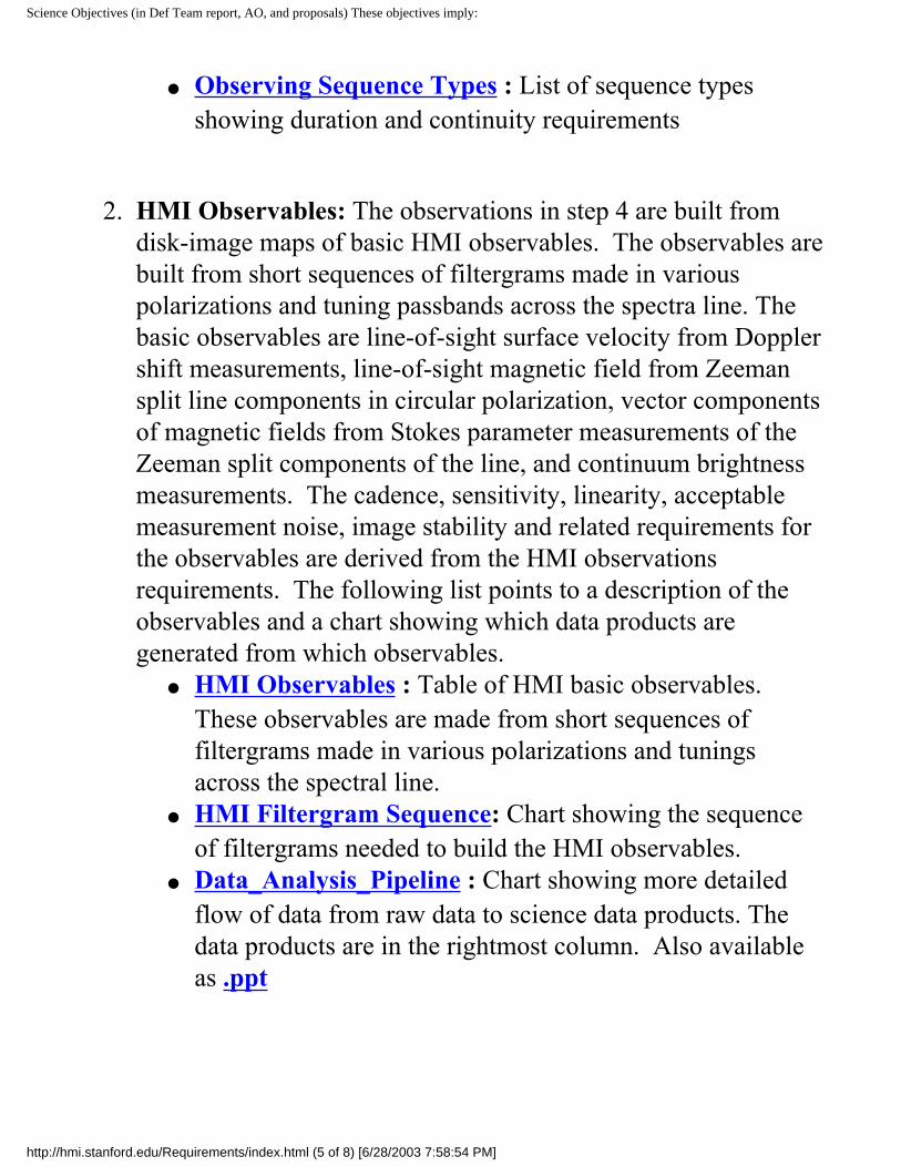
http://hmi.stanford.edu/Requirements

http://hmi.stanford.edu/doc/HMI_CSR/A_Sci_Plan/HMI_CSR_Requirements.pdf

Science Objectives (in Def Team report, AO, and proposals) These objectives imply:

HMI Requirements Flow PLEASE NOTE the requirements discussion is “living” document.In order to obtain the most up-to-date version please use this page:

http://hmi.stanford.edu/Requirements/Rather than a paper “snapshot” made at any particular moment. The HMI Investigation includes the HMI Instrument, data processing, and science analysis. There is a chain of objectives, goals, and requirements that flows from the top level science goals of LWS to specific requirements for performance of HMI and SDO space hardware. This list starts at the HMI objectives as "Step 1" and follows the chain to the spacecraft at "Step 9". The following is a description of the flow of requirements and goals from the top level science goals down to detailed requirements on instrument and analysis performance and on the SDO spacecraft. There is a natural chain of logic with some high level requirements having direct impacts on lower level systems. More often the requirements on lower level systems follow only after a detailed analysis of the implications of the higher level requirements. This top-level discussion starts at the most general and proceeds to the specific, in outline form. The requirements of each level imply the requirements on the lower levels. The numbers are not intended to correspond to NASA terminology of “Level-1” etc requirements (except where noted).

1. HMI Investigation: The top level objectives of the HMI Investigation flow directly from the science goals of SDO and LWS. These in turn flow from various NASA Roadmaps and NAS studies which represent the needs identified by the space

http://hmi.stanford.edu/Requirements/index.html (1 of 8) [6/28/2003 7:58:54 PM]


science community as a whole and the solar physics community in particular. The primary scientific objectives of the Helioseismic and Magnetic Imager (HMI) investigation are to improve understanding of the interior sources and mechanisms of solar variability and the relationship of these internal physical processes to surface magnetic field structure and activity. Details of the HMI “Level-1” requirements and background documents are in the following list.

HMI_Overview : HMI “Level-1” Requirements SDO Definition Team Report : SDO Definition Team

report, October 2001 (pdf, 56 pages) LWS Architecture Team Report : Report to SECAS, 30

August 2001 (pdf, 127 pages) NASA Roadmap 2000 : Contains SDO as “SONAR”

mission Astronomy and Astrophysics in the New Millennium :

NRC Report, 2001, html viewer.

2. HMI Science Objectives: The broad goals in step 1 are

approached in a number of more specific HMI Science Objectives. These include study of such topics as solar differential rotation, sub-surface flows around sunspots, emergence of magnetic flux in active regions, etc. These goals are described in the HMI Investigation proposal dated April 2002. These objectives will be met by analysis of HMI and related data with the results published in journals, conference proceedings and dissertations. In most cases new theory, modeling, simulation, and analysis techniques must be developed to accomplish the science objectives. HMI should be able to obtain the data needed for these objectives however the


http://hmi.stanford.edu/NASA_documents/lws_sdo_sdt_report.pdf

http://hmi.stanford.edu/NASA_documents/lws.sat_report2.pdf

http://hmi.stanford.edu/NASA_documents/roadmap2000.final_master.pdf

http://books.nap.edu/books/0309070317/html/


HMI investigation is not expected (nor proposed) to have sufficient resources to see all of the science objectives through to results and publications. The Co-I team (and the instrument team after 2 years on orbit) must seek other resources to complete the investigation. A summary of the HMI science objectives and background documents are in the following list.

HMI_Objectives.html : HMI Science Objectives Summary

Required Analysis, Simulation, and Modeling Techniques

HMI Proposal (April 2002) : .pdf files of HMI proposal

3. HMI Science Data Products: The analyses in step 2 require

specific data products as input to detailed analyses. These data products are not raw instrument observables but are rather often (usually for HMI) the result of substantial processing of time series of varying lengths. Examples are maps of subsurface flows, far-side active region maps, models of coronal fields, etc. A summary of these data products, a table showing the flow from science objectives to the data products and a chart showing the derivation of the data products from the processing pipeline are in the following list.

HMI Science_Data_Products : Summary of HMI science data products

Required Analysis/Processing Algorithm Development HMI_Objectives-Data_table : Matrix showing tie

between objectives to data products. Entries in this table show the observation sequence types required.

HMI science pipeline chart: Chart showing the flow of data from raw data to science data products to science


http://hmi.stanford.edu/proposal_April_2002/


objectives. Each arrow in this figure represents a matrix element from the above HMI Objectives-Data table. Also available as .ppt

1. HMI Observations: The data products in step 3 require specific

observation sequences providing data fulfilling specific requirements. These sequences are tailored to provide the data necessary for each of the data products above. Different data products imply differing requirements on observable, duration, completeness, noise, resolution, etc. This is the level at which time accuracy and continuity implications for the instrument and spacecraft data systems are first identifiable. Examples are 72d sequences of spherical harmonic amplitudes of solar surface velocity suitable for time series as source data for mode frequencies for internal rotation studies and 24h sequences of velocity in surface regions projected to particular mappings and tracked with time as source data for travel-time data-cubes suitable for sub-surface flow measurements. The “HMI Observations” are time series of maps of observables and intermediate products derived from them. Examples of observables are surface velocity and vector magnetic fields. In the tables below, the basic sequence parameters are identified apart from the observation sequences since some of the sequence types are used by more than one “HMI Observation” type. This distinction is made to allow identification of the requirements of the observation types apart from the continuity requirements for the sequences. The following list contains lists of HMI observation types, sequence types, and the chart showing the intermediate processing of the observation types.

Observation_types : List of observation types from which data products are built. Accuracy, resolution,


http://hmi.stanford.edu/Requirements/Science_Pipeline.ppt


Observing Sequence Types : List of sequence types showing duration and continuity requirements

2. HMI Observables: The observations in step 4 are built from

disk-image maps of basic HMI observables. The observables are built from short sequences of filtergrams made in various polarizations and tuning passbands across the spectra line. The basic observables are line-of-sight surface velocity from Doppler shift measurements, line-of-sight magnetic field from Zeeman split line components in circular polarization, vector components of magnetic fields from Stokes parameter measurements of the Zeeman split components of the line, and continuum brightness measurements. The cadence, sensitivity, linearity, acceptable measurement noise, image stability and related requirements for the observables are derived from the HMI observations requirements. The following list points to a description of the observables and a chart showing which data products are generated from which observables.

HMI Observables : Table of HMI basic observables. These observables are made from short sequences of filtergrams made in various polarizations and tunings across the spectral line.

HMI Filtergram Sequence: Chart showing the sequence of filtergrams needed to build the HMI observables.

Data_Analysis_Pipeline : Chart showing more detailed flow of data from raw data to science data products. The data products are in the rightmost column. Also available as .ppt


http://hmi.stanford.edu/Requirements/Data_Analysis_Pipeline.ppt


3. HMI Instrument Data: The MDI observables in step 5 are built from sequences of filtergrams. The filtergrams must be made in various polarizations, tuning positions, sequence order, optical configuration (i.e. observing or calibration) etc., to meet the functional requirements of the observable calculations and must be made with sufficient accuracy, noise levels, repeatability, timing knowledge, wavelength knowledge, image registration, image orientation, etc., to meet the science requirements. The table linked below lists the basic requirements on the filtergrams.

HMI Observables: List of basic requirements of filtergrams is also in the Observables requirements table.

4. HMI Instrument Concept: The required instrument data in step

6 will be obtained with the HMI instrument. The instrument concept was developed in an iterative process intended to result in a design concept which meets the requirements through step 6 and is achievable with real parts. The instrument is a system constructed of several subsystems. The requirements on the subsystems derive from the steps above with an understanding of the role of the subsystem within the instrument conceptual design.

HMI Instrument : The HMI instrument description from the April 2002 proposal

HMI Optics Layout: The HIM optical package plan. This diagram shows the locations of optics and mechanisms. This diagram shows what HMI is, not how to build it.

Sub-system requirements: Tables of implied requirements and estimated performance for subsystems including powered optics, image stabilization system, filter performance, tuning and polarization analyzer motors,


http://hmi.stanford.edu/proposal_April_2002/C.2_body.pdf


shutter, camera system, and data delivery system.

5. Sub-system design concepts:

6. HMI to SDO Interface Requirements: The SDO spacecraft

provides the home and environment for the HMI instrument. SDO should provide an environment and resources to enable steps 1 through 8 to be accomplished. The requirements on SDO have been encapsulated in the SDO Mission Requirements Document linked below. The top level requirements include support for HMI mass, power, telemetry needs as well as field-of-view, pointing direction and stability, thermal environment, etc.

HMI Resource Requirements Summary: Table of s/c

resources and environmental requirements Requirements FlowDown Summary : Summary showing

which S/C requirement derives from which of the above “steps”

SDO Mission Requirements Document: Draft MRD ver. 4.1 as of 9 Feb 2003.

7. Ground System:

8. Processing System:

9. Data Distribution:


http://hmi.stanford.edu/NASA_documents/SDO_MRD_4.1_2-9-03.html



BASIC REQUIREMENTS AND OBJECTIVES OF THE HELIOSEISMIC AND MAGNETIC IMAGER INVESTIGATION

Overview of Objectives and Requirements of the Helioseismic and Magnetic Imager Investigation The primary scientific objectives of the Helioseismic and Magnetic Imager (HMI) investigation are to improve understanding of the interior sources and mechanisms of solar variability and the relationship of these internal physical processes to surface magnetic field structure and activity. The HMI investigation is based on inferences to be made from measurements obtained by the HMI instrument as part of the Solar Dynamics Observatory (SDO) mission. The HMI instrument will make measurements of the dynamic motion of the solar photosphere on global and local solar scales to study solar surface oscillations and will make similarly scaled measurements of the polarization in a spectral line to study all three components of the photospheric magnetic field. HMI observations are crucial for establishing the relationships between the internal solar dynamics and related magnetic activity, leading to an understanding of the limits of and possible development of techniques for reliable predictive capability. Specific scientific objectives of the HMI investigation are to measure and study:

1. Convection-zone dynamics and the solar dynamo;2. Origin and evolution of sunspots, active regions and complexes

of activity;3. Sources and drivers of solar magnetic activity and disturbances;4. Links between the internal processes and dynamics of the

corona and heliosphere;5. Precursors of solar disturbances for space-weather forecasts.

http://hmi.stanford.edu/Requirements/HMI_Overview.html (1 of 2) [6/28/2003 7:58:59 PM]

BASIC REQUIREMENTS AND OBJECTIVES OF THE HELIOSEISMIC AND MAGNETIC IMAGER INVESTIGATION

To enable accomplishment of the science objectives of the investigation, the HMI instrument will produce measurements in the form of filtergrams in a set of polarizations and spectral line positions at a regular cadence for the duration of the mission that meet these basic requirements:

1. Full-disk Doppler velocity and line-of-sight magnetic flux images with 1.5 arc-sec resolution at least every 50 seconds.

2. Full-disk vector magnetic images of the solar magnetic field with 1.5 arc-sec resolution at least every 10 minutes.

The HMI data completeness and continuity requirement is to capture 99.99% of the HMI data 95% of the time. In addition, the HMI investigation will provide sufficient computing capability to convert these raw filtergram measurements into a set of observables and derived data products required for the HMI science objectives. The primary observables (Dopplergrams, longitudinal and vector magnetograms, and continuum intensity images) will be constructed from the raw filtergrams will be made available at full resolution and cadence. Other derived products such as subsurface flow maps, far-side activity maps, and coronal and solar wind models that require longer sequences of observations shall be produced and made available. All HMI data products will be made available to all interested investigators.

http://hmi.stanford.edu/Requirements/HMI_Overview.html (2 of 2) [6/28/2003 7:58:59 PM]

SDO - HMI Proposal

HMI Science Objectives.

This description of the HMI science objectives is extracted from the HMI proposal of April 2002.

C.1.2.1 Convection-zone dynamics and the solar dynamo

Fluid motions inside the Sun generate the solar magnetic field. Complex interactions between turbulent convection, rotation, large-scale flows and magnetic field produce regular patterns of solar activity changing quasi-periodically with the solar cycle. How are variations in the solar cycle related to the internal flows and surface magnetic field? How is the differential rotation produced? What is the structure of the meridional flow and how does it vary? What roles do the torsional oscillation pattern and the variations of the rotation rate in the tachocline play in the solar dynamo?

These issues are usually studied only in zonal averages by global Helioseismology but the Sun is longitudinally structured. Local helioseismology has revealed the presence of large-scale flows within the near-surface layers of the solar convection zone. These flows possess intricate patterns that change from one day to the next, accompanied by more gradually evolving patterns such as banded zonal flows and meridional circulation cells (Foldout 1.B, C). These flow structures have been described as Solar Subsurface Weather (SSW). Successive maps of these weather-like flow structures (Foldout 1.F) suggest that solar magnetism strongly modulates flow speeds and directions. Active regions tend to emerge in latitudes with stronger shear. The connections between SSW and active region development are presently unknown.

Structure and dynamics of the tachocline. Observation of the deep roots of solar activity in the tachocline is of primary importance for

http://hmi.stanford.edu/Requirements/HMI_Objectives.html (1 of 10) [6/28/2003 7:59:01 PM]

http://hmi.stanford.edu/proposal_April_2002/

SDO - HMI Proposal

understanding the long-term variability of the Sun. HMI will use global and local helioseismic techniques to observe and investigate the large-scale character of the convection zone and tachocline. Topics include solar differential rotation, relations between variations of rotation and magnetic fields, longitudinal structure of zonal flows (‘torsional oscillations’), relations between the torsional pattern and active regions, subsurface shear and its variations with solar activity, and the origin of the ‘extended’ solar cycle.

Variations in differential rotation. Differential rotation (Figure C.2) is a crucial component of the solar cycle and is believed to generate the global scale toroidal magnetic field in active regions. Results from MDI and GONG have revealed intriguing 1.3-year quasi-periodic variations of the rotation rate in the tachocline, which may be a key to understanding the solar dynamo. HMI will extend this key series with better near-surface resolution.

Evolution of meridional circulation. Precise knowledge of the meridional circulation in the convection zone is crucial for understanding the long-term variability of the Sun. Helioseismology has found evidence for variation of the internal poleward flow during the solar cycle. To understand the global dynamics we must follow the evolution of the flow. HMI will generate continuous data for detailed, 3-D maps of the evolving patterns of meridional circulation providing information about how flows transport and interact with magnetic fields throughout the solar cycle.

Dynamics in the near surface shear layer. Helioseismology has revealed that significant changes in solar structure over the solar cycle occur in the near-surface shear layer. However, the physics of these variations and their role in irradiance variations are still unknown. HMI will characterize the properties of this shear layer, the interaction between surface magnetism and evolving flow patterns,


SDO - HMI Proposal

and the changes in structure and dynamics as the solar cycle advances. It will assess the statistical properties of convective turbulence over the solar cycle, including the kinetic helicity and its relation to magnetic helicity – two intrinsic characteristics of dynamo action.

C.1.2.2 Origin and evolution of sunspots, active regions and complexes of activity

Observations show that magnetic flux on the Sun does not appear randomly. Once an active region emerges, there is a high probability that additional eruptions of flux will occur nearby (activity nests, active longitudes). How is magnetic flux created, concentrated, and transported to the solar surface where it emerges in the form of evolving active regions? To what extent are the appearances of active regions predictable? What roles do local flows play in their evolution?

HMI will address these questions by providing tracked sub-surface sound-speed and flow maps for individual active regions and complexes under the visible surface of the Sun combined with surface magnetograms. Current thinking suggests that flux emerging in active regions originates in the tachocline. Flux is somehow ejected from the depths in the form of loops that rise through the convection zone and emerge through the surface. Phenomenological flux transport models show that the observed photospheric distribution of the flux does not require a long-term connection to flux below the surface. Rather, field motions are described by the observed poleward flows, differential rotation, and surface diffusion acting on emerged flux of active regions. Does the active region magnetic flux really disconnect from the deeper flux ropes after emergence?

Formation and deep structure of magnetic complexes of activity.


SDO - HMI Proposal

HMI will explore the nature of long-lived complexes of solar activity (‘active or preferred longitudes’), the principal sources of solar disturbances. ‘Active longitudes’ have been a puzzle of solar activity for many decades. They may continue from one cycle to the next, and may be related to variations of solar activity on the scale of 1-2 years and short-term ‘impulses’ of activity. HMI will probe beneath these features to 0.7R, the bottom of the convection zone, to search for correlated flow or thermal structures.

Active region source and evolution. By using acoustic tomography we can image sound speed perturbations that accompany magnetic flux emergence and disconnection that may occur. Vector magnetograms can give evidence on whether flux leaves the surface predominantly as ‘bubbles’, or whether it is principally the outcome of local annihilation of fields of opposing polarity. With a combination of helioseismic probing and vector field measurements HMI will provide new insight into active region flux emergence and removal.

Magnetic flux concentration in sunspots. Formation of sunspots is one of the long-standing questions of solar physics.61-63 Recent observations from MDI have revealed complicated flow patterns beneath sunspots (Figure C.3) and indicated that the highly concentrated magnetic flux in spots is accompanied by converging mass flows in the upper 3-4 Mm beneath the surface (Foldout 1.J). The evolution of these flows is not presently known. Detailed maps of subsurface flows in deeper layers, below 4 Mm, combined with surface fields and brightness for up to 9 days during disk passage will allow investigation of the relations between flow dynamics and flux concentration in spots.

Sources and mechanisms of solar irradiance variations. Magnetic features - sunspots, active regions, and network - that alter the


SDO - HMI Proposal

temperature and composition of the solar atmosphere are primary sources of irradiance variability. How exactly do these features cause the irradiance variations? HMI together with the SDO Atmospheric Imaging Assembly (AIA) and Spectrometer for Irradiance (SIE), will study physical processes that govern these variations. The relation between interior processes, properties of magnetic field regions and irradiance variations, particularly the UV and EUV components that have a direct and significant effect on Earth’s atmosphere will be studied for the first time.

C.1.2.3 Sources and drivers of solar activity and disturbances

It is commonly believed that the principal driver of solar disturbances is stressed magnetic field. The stresses are released in the solar corona producing flares and coronal mass ejections (CME). The source of these stresses is believed to be in the solar interior. Flares usually occur in areas where the magnetic configuration is complex, with strong shears, high gradients, long and curved neutral lines, etc. This implies that the trigger mechanisms of flares are controlled by critical properties of magnetic field that lead eventually to MHD instabilities. But what kinds of instability actually govern, and under what conditions they are triggered are unknown. With only some theoretical ideas and models, there is no certainty of how magnetic field is stressed or twisted inside the Sun or just what the triggering process is.

Origin and dynamics of magnetic sheared structures and δ-type sunspots. The spots in Figure C.5 contain two umbrae of opposite magnetic polarity within a common penumbra and were the source of powerful flares and CMEs. Such δ-type sunspot regions are thought to inject magnetic flux into the solar atmosphere in a highly twisted state. It is important to determine what processes beneath the surface lead to development of these spots and allow them to become flare


SDO - HMI Proposal

and CME productive. This investigation will be carried out by analysis of evolving internal mass flows and magnetic field topology of such spots.

Magnetic configuration and mechanisms of solar flares. Vector magnetic field measurements can be used to infer field topology and vertical electric current, both of which are essential to understand the flare process. Observations are required that can continuously track changes in magnetic field and electric current with sufficient spatial resolution to reveal changes of field strength and topology before and after flares. HMI will provide these unique measurements of the vector magnetic field over the whole solar disk with reasonable accuracy and at high cadence.

Emergence of magnetic flux and solar transient events. Emergence of magnetic flux is closely related to solar transient events. MDI, GONG, and BBSO data show that there can be impulsive yet long-lived changes to the fields associated with eruptive events. Emergence of magnetic flux within active regions is often associated with flares. Emerging magnetic flux regions near filaments lead to eruption of filaments. CMEs are also found to accompany emerging flux regions. Further, emergence of isolated active regions can proceed without any eruptive events. This suggests that magnetic flux emerging into the atmosphere interacts with pre-existing fields leading to loss of magnetic field stability. Observations of electric current and magnetic topology differences between newly emerging and pre-existing fields will likely lead to the understanding of why emerging flux causes solar transient events. Vector polarimetry provided by HMI will enable these quantitative studies.

Evolution of small-scale structures and magnetic carpet. The quiet Sun is covered with small regions of mixed polarity, termed ‘magnetic carpet’ (Foldout 1.G), contributing to solar activity on


SDO - HMI Proposal

short timescales. As these elements emerge through the photosphere they interact with each other and with larger magnetic structures. They may provide triggers for eruptive events, and their constant interactions may be a source of coronal heating. They may also contribute to irradiance variations in the form of enhanced network emission. While HMI will certainly not see all of this flux, it will allow global scale observations of the small-scale element distribution, their interactions, and the resulting transformation of the large-scale field.

C.1.2.4 Links between the internal processes and dynamics of the corona and heliosphere

The highly structured solar atmosphere is predominately governed by magnetic field emerged from in the solar interior. Magnetic fields and the consequent coronal structures occur on many spatial and temporal scales. Intrinsic connectivity between multi-scale patterns increases coronal structure complexity leading to variability. For example, CMEs apparently interact with to the global-scale magnetic field, but many CMEs, especially fast CMEs, are associated with flares, which are believed to be local phenomena. Model-based reconstruction of 3-D magnetic structure is one way to estimate the field from observations. Models using vector field data in active regions provide the best match to the observations. More realistic MHD coronal models based on HMI high-cadence vector-field maps as boundary conditions will greatly enhance our understanding of how the corona responds to evolving, non-potential active regions.

Complexity and energetics of the solar corona. Observations from SOHO and TRACE have shown a variety of complex structures and eruptive events in the solar corona. However, categorizing complex structures has not revealed the underlying physics of the corona and coronal events. Two mechanisms have been proposed to generate


SDO - HMI Proposal

stressed magnetic fields: photospheric shear motions and emerging magnetic flux; and both may, in fact, be at work on the Sun. But which plays the dominant role and how the energy injection is related to eruptive events is unknown. Magnetic helicity is an important characteristic of magnetic complexity and its conservation intrinsically links the generation, evolution, and reconnections of the magnetic field. HMI will provide data to allow estimations of injections of energy and helicity into active regions the vector magnetic field and the velocity field (from helioseismology and correlation tracking). Observations from SDO AIA and White-light Coronagraphic Imager (WCI) will show the subsequent response and propagation of complexity into the corona and heliosphere, relating the build-up of helicity and energy with energetic coronal events such as CMEs.

Large-scale coronal field estimates. Models computed from line-of-sight photospheric magnetic maps have been used to reproduce coronal forms that show multi-scale closed field structures as well as the source of open field that starts from coronal holes but spreads to fill interplanetary space. Modeled coronal field demonstrates two types of closed field regions: helmet streamers that form the heliospheric current sheet and a region sandwiched between the like-polarity open field regions. There is evidence that most CMEs are associated with helmet streamers and with newly opened flux. HMI will provide uniform magnetic coverage at a high cadence, and together with simultaneous AIA, WCI and STEREO coronal images will enable the development of coronal field models and study of the relationship between pre-existing patterns, newly opening fields, long distance connectivity, and CMEs.

Coronal magnetic structure and solar wind. MHD simulation and current-free coronal field modeling based on magnetograms are two ways to study solar wind properties and their relations with coronal


SDO - HMI Proposal

magnetic field structure (Figure C.6). These methods have proven effective and promising, showing potential in applications of real-time space weather forecasting. It has been demonstrated that modeling of the solar wind can be significantly improved with increased cadence of the input magnetic data. By providing full-disk vector field data at high cadence, HMI will enable these models to describe the distribution of the solar wind, coronal holes and open field regions, and how magnetic fields in active regions connect with interplanetary magnetic field lines.

C.1.2.5 Precursors of solar disturbances for space-weather forecasts

Variations in the solar spectral irradiance and total irradiance may have profound effects on life through their potential but poorly understood role in climate changes. The variation from cycle to cycle of the number, strength, and timing of the strongest eruptive events is unpredictable at present. We are far from answering simple questions like ‘will the next cycle be larger than the current one?' 'When will the next large eruption occur?' Or even 'when will there be several successive quiet days?' As we learn more about the fundamental processes through studies of internal motions, magnetic flux transport and evolution, relations between active regions, UV irradiance, and solar shape variations we will be vigilant for opportunities to develop prediction tools. Nevertheless, there are several near term practical possibilities to improve the situation with HMI observations.

Far-side imaging and activity index. A procedure for solar far-side imaging was developed using data from MDI (Figure C.7), and has led to the routine mapping of the Sun’s far-side. Acoustic travel-time perturbations are correlated with strong magnetic fields, providing a view of active regions well before they become visible as rotate onto the disk at the east limb. Synoptic images, which are now able to


SDO - HMI Proposal

cover the entire far hemisphere of the Sun, will provide the ability to forecast the appearance of large active regions up to 2 weeks in advance and allow the detection of regions which emerge just a few days before rotating into view. HMI's full coverage to the limb will allow lower-noise far-side estimates.

Predicting emergence of active regions by helioseismic imaging. Rising magnetic flux tubes in the solar convection zone may produce detectable seismic signatures (Fig. C.4), which would provide warning of their impending emergence. Helioseismic images of the base of the convection zone will employ a similar range of p-modes as those used to construct images of the far side. A goal is to detect and monitor seismic signatures of persistent or recurring solar activity near the tachocline. Success here could lead to long-term forecasts of solar activity.

Determination of magnetic cloud Bs events. Potentially valuable information for geomagnetic forecasts - predictions of magnetic cloud Bs (southward field) events - can be obtained from the vector field measurements. Long intervals of large southward interplanetary magnetic field, Bs events, and high solar wind speed are believed to be the primary cause of intense geomagnetic disturbances with the Bs component the more important quantity. It has been shown that orientation in ‘clouds’ remains basically unchanged while propagating from the solar surface to Earth’s orbit. This provides a plausible chain of related phenomena that should allow prediction to be made from solar observations of the geo-effectiveness of CMEs directed toward Earth. Estimates of embedded Bs will be significantly improved by incorporating frequently updated vector field maps into coronal field projections with the potential addition of coronagraphic observations from AIA, WCI, and STEREO.


Scientific Data Products – Measurement Requirements

Scientific Data Products The scientific operation modes and data products can be divided into four main areas: global helioseismology, local-area helioseismology, line-of-sight and vector magnetography and continuum intensity studies. The principal data flows and products are summarized in the proposal in Foldout 1.L. These four primary scientific analyses cover all main HMI objectives, and have the following characteristics:

• Global Helioseismology: Diagnostics of global changes inside the Sun. The normal-mode method will be used to obtain large-scale axisymmetrical distributions of sound speed, density and flow velocities throughout the solar interior from the energy-generating core to the near-surface convective boundary layer. These diagnostics will be based on frequencies and frequency splittings of modes of angular degree (l) up to 1000, obtained for intervals of several days each month and up to l=300 for each 2-month interval. These will be used to produce a regular sequence of internal rotation and sound-speed inversions to allow observation of the tachocline and the near-surface shear layer.

• Local Helioseismology: 3D imaging of the solar interior. The time-distance technique, ring-diagram analysis and acoustic holography represent powerful tools for investigating physical processes inside the Sun. These methods are based on measuring local properties of acoustic and surface gravity waves, such as travel times, frequency and phase shifts. The targeted high-level regular data products include:

§ synoptic maps of mass flows and sound-speed perturbations in the upper convection zone for each Carrington rotation with a 2-degree resolution, from averages of full disk time-distance maps;

§ synoptic maps of horizontal flows in the upper convection zone for each Carrington rotation with a 5-degree resolution from ring-diagram analyses;

§ higher-resolution maps zoomed on particular active regions, sunspots and other targets, obtained with 4-8-hour resolution for up to 10-day transits;

§ deep-focus maps covering the whole convection zone depth, 0-200 Mm, with 10-15 degree resolution;

§ farside images of travel-time perturbations associated with large active regions every 12 hours.

These observations require uninterrupted series of Dopplergrams of lengths 8 to 24 hours with the following characteristics: 50-second (or higher) cadence, spatial sampling of 2 Mm for distances up to 75 degrees from the disk center, and the noise level better than 20 m/s.

• Magnetography. Complete coverage of magnetic processes in the photosphere. The traditional line-of-sight component of the magnetic flux is produced as a co-product with the

http://hmi.stanford.edu/Requirements/Science_Data_Products.html (1 of 7) [6/28/2003 7:59:03 PM]


Doppler velocity. Several products will be computed with various cadence (up to 10 minutes) and resolution for use as input to coronal field and solar wind models and correlative studies. To accurately model the global fields the zero point accuracy should be better than 0.1G.

•The vector magnetic field. This is one of the most important physical observables of the active solar atmosphere. HMI will produce several standard data series of vector fields. A simple ‘magnetograph mode’ analysis will be computed continuously in real time for large scale coronal modeling and other space weather applications. With help of inversion techniques113, HMI will also provide tracked and full-disk vector magnetic field, filling factor, and thermodynamic parameters of photospheric plasma within reasonable errors. The data will be used to measure free energy, stresses and helicity of the magnetic field, providing important input to many prime science objectives and tasks of HMI and other SDO investigations. These polarimetric observations require a few minutes temporal cadence, a spatial sampling of 0.5”, and a 0.3% polarization precision to yield 5% accuracy of the magnetic field strength, a few tens of degrees in inclination and azimuth in strong fields.

• Continuum Intensity: Identification of irradiance sources. The observations of the intensity in the continuum near the HMI spectral line will give a very useful measure of spot, faculae area and other sources of irradiance. This will be important for studying the relationship between the MHD processes in the interior and lower atmosphere and irradiance variations. The continuum data will be also used for limb shape analysis, and for public information and education purposes. These measurements require calibration of system pixel-pixel gain variations to a level 0.1%, as demonstrated with MDI.

HMI Science Data Measurements. The data observing sequences that are used as input for analyses are described here as a number of observation types. The Observation Types that support the various science objectives are shown in the HMI_Objectives-Data_table. The Observation Types are described here. NOTE THESE PAGES ARE STILL UNDER REVIEW

Observation Type HS-1 Global HS synoptic uses typically 72-day intervals. Repeated intervals are needed to follow solar variations with changes in solar activity. Loss of a few intervals in a three year span would still yield important results to extend the SOHO/MDI results into the next cycle. If GONG continues into the SDO mission years these observations have a somewhat lower



priority since higher-noise but still very useful data can be obtained with GONG. In the past seven years GONG has (in 36-day intervals) coverage in the range of 70 to 85% (of the minutes). MDI has typically 96-97% coverage except of course for the large gaps. For low-degree (less than l=120) modes we believe most of the noise difference results from coverage completeness. We believe that coverage less than ninety something percent results in noticeable noise, probably the limit is about 90. We believe that solar noise is such that the noise in the frequency fits with coverage between about 95% and 100% is indistinguishable. Thus 95% is a good place to be sure that we are limited by solar noise rather than noise from data gaps. Where there are gaps we have found that random times of random sizes is least damaging. Gap filling methods can recover most of the signal when the gap is less than 10% of the surrounding spans of more complete data. Gaps of less than half the Nyquist sampling interval of the 5.3 mHz acoustic cutoff frequency have little if any effect when we use the MDI processing method of no-trend removal. Using the GONG method of first differences puts a tighter constraint on small gaps. 5.3 mHz is a period of 3.1 minutes. This leads to a maximum harmless gap of about 90 seconds (two HMI sample intervals) for global HS data. Observation Type Table EntryType Observing

SequenceNeeded

ObservablesPlanned Span of Observations

Planned Number of Observations (percent coverage)

MinimumSpan of Observations

MinimumNumber of Observations (percent coverage)

MinimumImage resolution

Notes

HS-1 OS-1 fd_V, fd_Ic

5-years 25 (100%) 3-years 12 (80%) 2” Global structure and rotation

Observing Sequence Type Table EntryObservingSequence Type

Nominal Interval

Completeness in interval

Max harmless gap

OptimumGap distribution

Notes

OS-1 72d 95% 90s random

Observation Type HS-2 Global Scale Local Method Helioseismology. HS-2. This type of observation supports measurement of deep-in-the-Sun flows and possibly fields. The method uses time-distance techniques to probe the conditions in the vicinity of the tachocline and bottom of the convection zone. This is about 200Mm deep. The end-points of acoustic rays that turn at this depth are about 700Mm apart, i.e. about a solar radius. This means that only a narrow range of longitude or latitude from disk center can be probed. With end points about 60 degrees apart



and limiting data to about 75 degrees from disk center (0.96R where projection factor is about 4) the distance from disk center at the turning point is at most about 45 degrees. A “point” could then be tracked for 90 degrees or about 6 days. Doppler noise near the limb may restrict the range to +-60 degrees (0.87R, factor of 2 in projection) giving a 60 degree or 4 day maximum observing sequence. Experiments have shown useful S/N for one day sequences .Due to the wavelength of waves at the tachocline (c. 70Mm) the maximum resolution achievable is about 10 degrees. Thus about 5 resolution elements are detectable for each day-long sequence and 36 elements covers a rotation. This means the minimum requirement is 8 one-day sequences per month with at most 4-day gaps. Type Observing

SequenceNeeded






Notes

HS-2 OS-2 fd_V

5-years 1800 (98%)allows 5 lost days/yr

3-years 300 with max gap of 4 days (25%)

2” Tachocline structure from time-distance


Nominal Interval


Max harmless gap


Notes

OS-2 24h 85% 90s bunched

Observation Type HS-3 Sub-Surface “Weather” – SSW. This type of observation supports both Time-Distance and Ring type analyses (as well as holographic techniques). The goal is to study the region from the surface to 30Mm in detail and watch global and AR scale flows as they evolve. Sequences of a day are tracked in data cubes of typically 15-degrees or 7.5 degrees (perhaps 5 degrees with HMI). The Sun’s disk is tiled with overlapping tracked cubes and flow analysis is performed on each cube. MDI has shown changes on day time scales with larger scales persistent for rotations (or years in case of zonal flows a.k.a. torsional oscillations). MDI has only allowed one 2-rotation sequence per year. This is not sufficient to determine the persistence or nature of evolution of active region scale or even radius-scale flows. We believe a minimum of three contiguous rotations at least once each six months would yield important data on these flows. We should sample over the full rising part of the cycle – i.e. from min to max. The base plan is for continual mapping.



Type Observing SequenceNeeded






Notes

HS-3 OS-3 fd_V

5-years 20 (100%) Min to max 6 – one 3-rotation sequence each 6 months

2” Large scale subsurface “weather”


Nominal Interval


Max harmless gap


Notes


Observation Type HS-4 Active Longitude Studies. This observation type will provide data for the examination of the source of active zones or longitudes or complexes of activity. We know a good deal statistically about the clumpiness of activity but do not know of any internal cause for such clumping. This study will use techniques nearly identical to HS-3 except that longer contiguous spans are required. We believe we need at least 4-rotation spans of synoptic maps of sub-surface flows. Both Ring and Time-Distance analyses will be applied. Time-Distance prefers clumped gaps and Rings prefer random gaps. Type Observing

SequenceNeeded






Notes

HS-4 OS-4 fd_V

5-years 15 (100%) 3-years 5 four-rotation sequences (55%)

2” Active Longitudes


Nominal Interval


Max harmless gap


Notes




Observation Type HS-5 Active Region Studies. This observation type produces data to allow study of flows, thermal, and field structure beneath active regions. Both Time-Distance and Holographic methods will be used. Since the details in the near surface layers are important the highest resolution data will be needed. The wavelength of acoustic waves near the surface is about 2Mm and this sets a natural resolution target. Active regions have lifetimes of weeks to months. If data is used to about 0.93 R then a 1Mm pixel subtends 0.5”. This gives a 10-day span of coverage. 12-days coverage with 0.5” pixels corresponds to 2Mm pixels with data used out to 0.98R. We would hope to obtain clean data for 10-day spans with analyses extended to 12-day spans with allowances for lower resolution at the ends. This means we can observe 20-50% of the lifetime of many active regions with full coverage of many short lived small regions. With this coverage we should be able to determine the flow-evolution from prior to eruption to post-visibility for small, typical, and a few large regions. We estimate that a sample of 100 regions tracked for 12-days each will yield at least 10 large region segments and we consider this to be a minimum requirement for this study. The baseline plan calls for tracking all active regions with NOAA identification. 100 regions can be captured in about 2.5 years starting at minimum or in less than six months near a typical maximum of activity. Since Time-Distance methods will be used gaps should be clumped into as few sub-intervals as possible. Ring type analyses do not give enough resolution for these studies. TypeObserving

SequenceNeeded






Notes

HS-5

OS-5 fd_V

5-years 100% 2.5-years starting at min or 1 year at max

100 regions2” Active Regions,Multiple regions concurrently


Nominal Interval


Max harmless gap


Notes

OS-5 12d 95% 90s clumped




Table showing relationship between HMI science objectives (Proposal section C1) and data products (Proposal Foldout.1 Section L)

Inte

rnal

rota

tion Ω

(r,Θ

) (0<

r<R

)

Inte

rnal

soun

d sp

eed,

cs(

r,Θ) (

0<r<

R)

Full-

disk

vel

ocity

, v(r

,Θ,Φ

), A

nd so

und

spee

d, c

s(r,Θ

,Φ),

Map

s (0-

30M

m)

Car

ringt

on sy

nopt

ic v

and

cs m

aps (

0-30

Mm

) H

igh-

reso

lutio

n v

and

cs m

aps (

0-30

Mm

)

Dee

p-fo

cus v

and

cs m

aps (

0-20

0Mm

)

Far-

side

act

ivity

inde

x Li

ne-o

f-Si

ght M

agne

tic fi

eld

map

s V

ecto

r Mag

netic

Fie

ld m

aps

Cor

onal

mag

netic

Fie

ld e

xtra

pola

tions

C

oron

al a

nd S

olar

win

d m

odel

s

Brig

htne

ss Im

ages

Con

text

Mag

neto

gram

s

EUV

Imag

es, i

.e. A

IA

Cor

onag

raph

Imag

es

EUV

Spe

ctra

l Irr

adia

nce

Structure and dynamics of the tachocline

HS-1

HS-1 HS-2 MAG

-1

Variations in differential rotation

HS-1 HS-3 HS-

3 HS-2 MAG-1

Evolution of meridional circulation

HS-3 HS-3

HS-3 HS-2 MAG

-1

Convection zone dynamics and solar dynamo

Dynamics in the near surface shear layer

HS-3 HS-3 HS-

3 HS-

3 MAG-1

Formation and deep structure of magnetic complexes of activity

HS-4

HS-4 HS-

2 MAG

-1 MAG-2

Active region source and evolution HS-5 HS-

5 HS-

5 HS-2

MAG-3

Magnetic flux concentration in sunspots

HS-5 HS-5

HS-5 MAG

-3

Origin and evolution of sunspots, active regions and complexes of activity

Sources and mechanisms of solar irradiance variations

HS-6 HS-6 HS-6 MAG

-1 MAG

-1 IC-

1 X X

Origin and dynamics of magnetic sheared structures and δ-type sunspots

HS-8 MAG

-4 MAG

-4

IC-2

Magnetic configuration and mechanisms of solar flares

MAG-5

MAG-4

MAG-2

X X

Emergence of magnetic flux and solar transient events.

HS-5 MAG

-3 MAG

-3 MAG

-3

X

Sources and drivers of solar activity and disturbances

Evolution of small-scale structures and magnetic carpet

MAG-6 MAG

-1 MAG

-6

X

Table showing relationship between HMI science objectives (Proposal section C1) and data products (Proposal Foldout.1 Section L)

Inte

rnal

rota

tion Ω

(r,Θ

) (0<

r<R

)

Inte

rnal

soun

d sp

eed,

cs(

r,Θ) (

0<r<

R)

Full-

disk

vel

ocity

, v(r

,Θ,Φ

), A

nd so

und

spee

d, c

s(r,Θ

,Φ),

Map

s (0-

30M

m)

Car

ringt

on sy

nopt

ic v

and

cs m

aps (

0-30

Mm

) H

igh-

reso

lutio

n v

and

cs m

aps (

0-30

Mm

)

Dee

p-fo

cus v

and

cs m

aps (

0-20

0Mm

)

Far-

side

act

ivity

inde

x Li

ne-o

f-Si

ght M

agne

tic fi

eld

map

s V

ecto

r Mag

netic

Fie

ld m

aps

Cor

onal

mag

netic

Fie

ld e

xtra

pola

tions

C

oron

al a

nd S

olar

win

d m

odel

s

Brig

htne

ss Im

ages

Con

text

Mag

neto

gram

s

EUV

Imag

es, i

.e. A

IA

Cor

onag

raph

Imag

es

EUV

Spe

ctra

l Irr

adia

nce

Complexity and energetics of the solar corona

MAG-7 HS-3 MAG

-7 MAG-7

MAG-7 X X

Large-scale coronal field estimates MAG

-8 MAG-8

X X

Links between the internal processes and dynamics of the corona and heliosphere Coronal magnetic

structure and solar wind

MAG-8

MAG-8

MAG-8

X X

Far-side imaging and activity index X X X X

Predicting emergence of active regions by helioseismic imaging

X X X X X

X Precursors of solar disturbances for space-weather forecasts

Determination of magnetic cloud Bs events

X X

X

A new description of the Observation Types (e.g. HS-1) is being developed and is in this directory as Observation_types.doc and Observation_types.html.

http://hmi.stanford.edu/Requirements/Observation_types.doc

Observation Observable, object

Instances or % of intervals

Observing interval


Span of observations

Res Notes

HS-1 V, fd 12 72-day 95% 3-years 2” HS-2 V, fd 80% 24-hour 85% 3-years 2” HS-3 V, fd 2 90-day 95% Min-max 2 per year HS-4 V, ARs 5 120-day 95% Active Sun HS-5 V, ARs 100 12-day 95% Any 1” >10

“large” HS-6 V, fd 60% 24-hour 95% Min-max 2” Max gap

30h HS-7 V, fd 80% 10-hour 95% Min-max 1” Max gap

30h HS-8 V, ARs >5 delta-

spots 10-day 95% Any Need to

sample several at all phases of life

MAG-1 B-5m, fd 80% 5-min/hour 80% 3-years 2” Max gap 10h

MAG-2 B-5m, fd 10% 5-min/hour 80% 3-years 2” Min 2/day MAG-3 B, ARs 100 12-day 95% Any 1” >10

“large” MAG-4 B, ARs >5 delta-

spots 10-day 95% Any

MAG-5 B, ARs 50 ARs with flares

2-day 95% Any >2 X-class

MAG-6 B, fd Monthly 3-day Min-max MAG-7 B,fd 50% 60-day 85% for HS Min-max MAG-8 B or Bvec 3 per day

80% of time

20-min Min-max

IC-1 Ic,fd 80% 5-min/hour 80% 3-years 2” Max gap 10h

IC-2 >5 delta spots

10-day 95% Min-max

http://hmi.stanford.edu/Requirements/Science_Pipeline.jpg

http://hmi.stanford.edu/Requirements/Science_Pipeline.jpg [6/28/2003 7:59:07 PM]

http://hmi.stanford.edu/Requirements/Observation_types.html

HMI Science Data Measurements. The data observing sequences that are used as input for analyses are described here as a number of observation types. The Observation Types that support the various science objectives are shown in the HMI_Objectives-Data_table. The Observation Types are described here. NOTE THESE PAGES ARE STILL UNDER REVIEW

Observation Type HS-1 Global HS synoptic uses typically 72-day intervals. Repeated intervals are needed to follow solar variations with changes in solar activity. Loss of a few intervals in a three year span would still yield important results to extend the SOHO/MDI results into the next cycle. If GONG continues into the SDO mission years these observations have a somewhat lower priority since higher-noise but still very useful data can be obtained with GONG. In the past seven years GONG has (in 36-day intervals) coverage in the range of 70 to 85% (of the minutes). MDI has typically 96-97% coverage except of course for the large gaps. For low-degree (less than l=120) modes we believe most of the noise difference results from coverage completeness. We believe that coverage less than ninety something percent results in noticeable noise, probably the limit is about 90. We believe that solar noise is such that the noise in the frequency fits with coverage between about 95% and 100% is indistinguishable. Thus 95% is a good place to be sure that we are limited by solar noise rather than noise from data gaps. Where there are gaps we have found that random times of random sizes is least damaging. Gap filling methods can recover most of the signal when the gap is less than 10% of the surrounding spans of more complete data. Observation Type Table EntryType Observing

SequenceNeeded






Notes

HS-1 OS-1 fd_V, fd_Ic

5-years 25 (100%) 3-years 12 (80%) 2” Global structure and rotation

Observing Sequence Type Table Entry

http://hmi.stanford.edu/Requirements/Observation_types.html (1 of 6) [6/28/2003 7:59:08 PM]


ObservingSequence Type

Nominal Interval


Max harmless gap


Notes


Observation Type HS-2 Global Scale Local Method Helioseismology. HS-2. This type of observation supports measurement of deep-in-the-Sun flows and possibly fields. The method uses time-distance techniques to probe the conditions in the vicinity of the tachocline and bottom of the convection zone. This is about 200Mm deep. The end-points of acoustic rays that turn at this depth are about 700Mm apart, i.e. about a solar radius. This means that only a narrow range of longitude or latitude from disk center can be probed. With end points about 60 degrees apart and limiting data to about 75 degrees from disk center (0.96R where projection factor is about 4) the distance from disk center at the turning point is at most about 45 degrees. A “point” could then be tracked for 90 degrees or about 6 days. Doppler noise near the limb may restrict the range to +-60 degrees (0.87R, factor of 2 in projection) giving a 60 degree or 4 day maximum observing sequence. Experiments have shown useful S/N for one day sequences .Due to the wavelength of waves at the tachocline (c. 70Mm) the maximum resolution achievable is about 10 degrees. Thus about 5 resolution elements are detectable for each day-long sequence and 36 elements covers a rotation. This means the minimum requirement is 8 one-day sequences per month with at most 4-day gaps. Type Observing

SequenceNeeded






Notes

HS-2 OS-2 fd_V

5-years 1800 (98%)allows 5 lost days/yr

3-years 300 with max gap of 4 days (25%)

2” Tachocline structure from time-distance


Nominal Interval


Max harmless gap


Notes

OS-2 24h 85% 90s bunched

Observation Type HS-3



Sub-Surface “Weather” – SSW. This type of observation supports both Time-Distance and Ring type analyses (as well as holographic techniques). The goal is to study the region from the surface to 30Mm in detail and watch global and AR scale flows as they evolve. Sequences of a day are tracked in data cubes of typically 15-degrees or 7.5 degrees (perhaps 5 degrees with HMI). The Sun’s disk is tiled with overlapping tracked cubes and flow analysis is performed on each cube. MDI has shown changes on day time scales with larger scales persistent for rotations (or years in case of zonal flows a.k.a. torsional oscillations). MDI has only allowed one 2-rotation sequence per year. This is not sufficient to determine the persistence or nature of evolution of active region scale or even radius-scale flows. We believe a minimum of three contiguous rotations at least once each six months would yield important data on these flows. We should sample over the full rising part of the cycle – i.e. from min to max. The base plan is for continual mapping. One important component of large scale solar flows are the meridional or poleward flows. They have typical amplitudes of several m/s. We should be able to detect real variations down to c. 1 m/s. To avoid leakage of the 2 km/s solar rotation signal into the meridional signal we must know the roll orientation to better than 2 arc-min. Type Observing

SequenceNeeded






Notes

HS-3 OS-3 fd_V

5-years 20 (100%) Min to max 6 – one 3-rotation sequence each 6 months

2” Large scale subsurface “weather”


Nominal Interval


Max harmless gap


Notes


Observation Type HS-4 Active Longitude Studies. This observation type will provide data for the examination of the source of active zones or longitudes or complexes of activity. We know a good deal statistically about the clumpiness of activity but do not know of any internal cause for such



clumping. This study will use techniques nearly identical to HS-3 except that longer contiguous spans are required. We believe we need at least 4-rotation spans of synoptic maps of sub-surface flows. Both Ring and Time-Distance analyses will be applied. Time-Distance prefers clumped gaps and Rings prefer random gaps. Type Observing

SequenceNeeded






Notes

HS-4 OS-4 fd_V

5-years 15 (100%) 3-years 5 four-rotation sequences (55%)

2” Active Longitudes


Nominal Interval


Max harmless gap


Notes


Observation Type HS-5 Active Region Studies. This observation type produces data to allow study of flows, thermal, and field structure beneath active regions. Both Time-Distance and Holographic methods will be used. Since the details in the near surface layers are important the highest resolution data will be needed. The wavelength of acoustic waves near the surface is about 2Mm and this sets a natural resolution target. Active regions have lifetimes of weeks to months. If data is used to about 0.93 R then a 1Mm pixel subtends 0.5”. This gives a 10-day span of coverage. 12-days coverage with 0.5” pixels corresponds to 2Mm pixels with data used out to 0.98R. We would hope to obtain clean data for 10-day spans with analyses extended to 12-day spans with allowances for lower resolution at the ends. This means we can observe 20-50% of the lifetime of many active regions with full coverage of many short lived small regions. With this coverage we should be able to determine the flow-evolution from prior to eruption to post-visibility for small, typical, and a few large regions. We estimate that a sample of 100 regions tracked for 12-days each will yield at least 10 large region segments and we consider this to be a minimum requirement for this study. The baseline plan calls for tracking all active regions with NOAA identification. 100 regions can be captured in about 2.5 years starting at minimum or in less than six months near a typical maximum of activity. Since Time-Distance methods will be used gaps should be clumped into as few sub-intervals as possible. Ring type analyses do not give enough resolution for these studies.



TypeObserving

SequenceNeeded






Notes

HS-5

OS-5 fd_V

5-years 100% 2.5-years starting at min or 1 year at max

100 regions2” Active Regions,Multiple regions concurrently


Nominal Interval


Max harmless gap


Notes

OS-5 12d 95% 90s clumped

Observation Type MAG-3 FACTS:Nature of emerging magnetic flux: emerging of active regions; emerging magnetic flux within active regions.Observation of emerging magnetic flux: quickly emerge firstly (in the first 30 minutes), slow down in the coming 6 hours, and stop after 10 hours; strong transverse component of magnetic field; downflows seen at footpints; flux emerging within active regions often associated with flaring activity which is limited to the procedure of emerging; whether emerging of active regions causing eruption of nearby filaments depends on orientations of newly active regions and background field (favor for reconnection). Tasks: process of emergence of magnetic flux within active regions; emerging of active regions (structure of emerging magnetic field – Omega or U loops, energy buildup, and adjustment of magnetic configuration by rotation, motion to follow Hale law with vector and line-of-sight magnetograms, brightness and EUV images); structure of emerging flux regions (structure & topology of magnetic field inferred and computed by vector data, EUV observation, and coronal field extrapolation); interaction of newly emerging flux and pre-existed field (both in small-scale and large-scale) in order to understand its role for flare, eruption of filaments, and/or CMEs; formation, structure, stability of filaments: (1) formation (as short as 15 min, reappearance after eruption in one hour or less, test scenarios of shear motion, reconnection, twisted-already before emerging by using vector field data, brightness images and EUV images); (2) magnetic configuration (structure & topology from vector field data & EUV data);(3) stability (kink instability: buildup of twist by shear motion or by merging of newly



emerged, twisted-already fluxes, based on vector data, brightness & EUV images). REQUIREMENTS:Samples: more than 5 examples for emerging of active regions, emerging flux regions within active regions, emerging of active regions near filaments (within 20 degree).Observations: vector magnetic field (accuracy for transverse component and azimuth angle is of high priority; 10 min cadence; 2 arcsec resolution); line-of-sight magnetograms (1 min cadence; 2 arcsec resolution; for detecting emerging and evolution of magnetic flux such as motion, cancellation, etc.); brightness images (1 min cadence for LCT); EUV (temporal, spatial resolution is of priority, no worse than 10 min cadence, 2 arcsec resolution to discern structure and behavior of emerging for magnetic flux, longer than 1 hour duration); coronagraph images( temporal resolution is of priority- no worse than 10 minutes for inner coronal images; longer than 1 hour interval). Calculation: coronal magnetic extrapolation (10 minutes cadence); coronal and solar wind models (60 minutes cadence).

For other magnetic field observation types, see the “green” text in Magnetic_ObjectivesThese items will be incorporated into this document soon (12 Mar ’03)


Page 18SDO System Requirements Review/System Concept Review (SRR/SCR) – April 8-10, 2003

HMI Observables Requirements - 1

Packet loss: 0.01%99.99% complete95% of the time

99% complete 95% of the time

1.2.11.2.2

CCD pixels: 40962FOV: 2000” x 2000”Full disk3.2.2

CCD pixels: 40962Square pixels 0.5”

Jitter: 0.1”

Aperture: 14cmAngular resolution: 1.5(1.0)”Angular resolution: 1.5(1.0)”

1.3.11.3.23.2.1

InstrumentFiltergramObservableMRD

General Requirements

Offset pointingFlat field knowledgePixel to pixel accuracy: 0.1%

2.5.8.5

Full well: 125ke-Intensity noise: 0.3%Noise: 0.3%

CCD readout speed: 3.4sI framelist: 50(45)sCadence: 50(45)s


Continuum Intensity Requirements

Numbers in () are goals. *indicates TBD. Most numbers are 1σ.



Velocity Requirements

CCD readout speed: 3.4sFiltergrams @ 5 or 6 λ

3 tuned elementsTuning range: ±250 mÅRange: ±6.5km/s(and ±3kG)

1.5.1

Filter uniformity, drift

HCM accuracy: 10’λ accuracy: 3 mÅAbsolute: 10* m/s2.1

Orbit informationEffective λ knowledge

Two camerasEach cycle same λ’s

Shutter: 50(5)µsExposure knowledge: 200(20)ppm

HCM repeatability: 60(6)”λ repeatability: 0.3(0.03) mÅDisk averaged noise: 1(0.1)* m/s

3.2.35.2.5.4

Element widths

7 elementsSmall sidelobes

Element widthsFilter width: 76 mÅ

Full well: 30(125)ke-Intensity noise: 0.6(0.3)%Noise: 25(13)m/s1.5.1

CCD readout speed: 3.4sV framelist: 50(45)sCadence: 50(45)s1.6.1InstrumentFiltergramObservableMRD



Line-of-sight Field Requirements

CCD readout speed: 3.4sFiltergrams @ 5 or 6 λ

3 tuned elementsTuning range: ±250mÅRange: ± 3(4)kG(and ± 6.5km/s)

1.5.4

Shutter: 30(20)µsExposure knowledge: 120(80)ppm

HCM repeatability: 36(24)” or No move LCP↔RCP

λ repeatability: 0.18(0.12) mÅZero point: 0.3(0.2)G1.5.2FeI 6173Å (g=2.5)High effective Landé g

Full well: 40(125)ke-Intensity noise: 0.5(0.3)%Noise: 17(10)G1.5.3LCP & RCP availableLCP+RCP each cycle

CCD readout speed: 3.4sLOS framelist: 50(45)sCadence: 50(45)s1.6.2InstrumentFiltergramObservableMRD

Vector Field Requirements

Full well: 70(125)ke-Intensity noise: 0.4(0.3)%Polarization: 0.3(0.22)%

1.5.54 states available4 states each cycle

CCD readout speedVector framelist: 600(90)sCadence: 600(90)s1.2.41.6.3


http://hmi.stanford.edu/Requirements/Filtergram_Sequence_1.0.jpg

http://hmi.stanford.edu/Requirements/Filtergram_Sequence_1.0.jpg [6/28/2003 7:59:10 PM]

http://hmi.stanford.edu/Requirements/Data_Analysis_Pipeline.jpg

http://hmi.stanford.edu/Requirements/Data_Analysis_Pipeline.jpg [6/28/2003 7:59:11 PM]


HMI Subsystems• Optics Package Structure

– The optic package subsystem includes the optics package structure, optical components mounts and legs that attach the optics package to the spacecraft.

• Optics Subsystem– Includes all the optical elements except the filters.

• Filter subsystem– The filter subsystem includes the front window, blocking filter, Lyot filter and Michelson interferometers– Provides the ability to select the wavelength to image

• Thermal Subsystem– Controls the temperature of the optics package, the filter oven, CCDs, and the front window.– Implements the decontamination heating of the CCD.

• Image Stabilization Subsystem– Consists of active mirror, limb sensor, precision digital & analog control electronics– Actively stabilizes the image reducing the effects of jitter

• Mechanisms Subsystem– The mechanisms subsystem includes shutters, hollow-core motors, calibration/focus wheels, alignment

mechanism, and the aperture door.

• CCD Camera Subsystem– The CCD camera subsystem includes 4Kx4K CCDs and the camera electronics box(es).

• HMI Electronics Subsystem– Provides conditioned power and operation of all HMI subsystems as well as HMI C&DH hardware.

• Software Subsystem– The software subsystem includes the C&DH spacecraft interface and control of HMI subsystems


HMI Optics Package Layout


Optics Subsystem

• 1 arc-sec diffraction limited image at the sensor– Requires 14 cm aperture– Requires 4096x4096 pixel sensor

• Solar disk at the sensor 4.9 cm– For sensor with 12 um pixels

• Focus adjustment system with ±3 (TBC) depth of focus range and 16 steps• Provide calibration mode that images the pupil on the sensor• Provide beam splitter to divide the telescope beam between the filter oven and

the limb tracker• Provide telecentric beam through the Lyot filter• Provide beam splitter to feed the output of the filter subsystem to two sensors• Minimize scattered light on the sensor


Filter subsystem

• Central wavelength 6173Å Fe I line• Reject 99% of solar heat load from the OP interior• Total bandwidth 76 mÅ FWHM• Tunable range 500 mÅ• Wavelength selection stability and repeatability of 0.18 mÅ• The required bandwidth obtained by cascading filters as follows

– Front window 50Å– Blocker 8Å– Lyot filter (5 element 1:2:4:8:16) 306 mÅ– Wide Michelson 172 mÅ– Narrow Michelson 86 mÅ

• Tuning range requires use of three co-tuned elements– Narrowest Lyot element– Wide Michelson– Narrow Michelson


MDI Lyot Elements and Michelson Interferometers


Thermal Subsystem

• Optics package thermal control– Operating temperature range 15 to 25 °C– Active control to ± 0.5 °C – Control loop in software

• Filter oven– Operating temperature range 35 ± 4 °C– Temperature accuracy 0.5 °C– Temperature stability 0.01 °C /hour– Changes in internal temperature gradients as small as possible– Dedicated analog control loop in controlled thermal environment

• Sensor (CCD detector) thermal control– Operating –100 °C to –30 °C– Decontamination mode raises CCD to between 20 °C and 40 °C

• Front window thermal control– Minimize radial gradients– Return to normal operating temperature within 60 minutes of eclipse exit


Image Stabilization Subsystem

• Stability is 0.1 arc-sec over periods of 90 seconds (TBC)• Range ± 14 arc-sec• Frequency range 0 to 50 Hz• Continuous operation for life of mission


Mechanisms (1 of 2)

Shutters• Repeatability 100 us• Exposure range 50 ms to 90 sec• Knowledge 30 us• Life (5 year) 40 M exposures

Hollow core motors• Move time (60 deg) < 800 ms• Repeatability 60 arc-sec• Accuracy 10 arc-min• Life (5 year) 80 M moves


Mechanisms (2 of 2)

Calibration / focus wheels• Positions 5• Move time (1 step) 800 ms• Accuracy TBD arc-min• Repeatability TBD arc-min• Life (5 Years) 20 K moves

Alignment system• Movement range ± 200 arc-sec• Step size 2 arc-sec

Aperture door• Robust fail open design


CCD Camera Subsystem

• Format 4096 x 4096 pixels• Pixel size 12 um• Full well > 125K electrons• Readout noise 40 electrons• Readout time < 3.4 seconds• Digitization 12 bits• Dark current 10 –e/sec/pixel at -60 °C


HMI Electronics Subsystem

• Provide conditioned power and control for all HMI subsystems• Provide processor for:

– Control all of the HMI subsystems– Decoding and execution of commands– Acquire and format housekeeping telemetry– Self-contained operation for extended periods– Program modifiable on-orbit

• Provide stable jitter free timing reference • Provide compression and formatting of science data• Provide dual interface for 55 Mbps of science date • Provide spacecraft 1553 interface

– Commands 2.0 kbps– Housekeeping telemetry 2.5 kbps– Diagnostic telemetry 10 kbps for short periods upon request


HMI Electrical Block Diagram


Software Subsystem

• The HMI flight software will perform the following functions– Process commands from spacecraft– Acquire and format housekeeping telemetry– Store and execute operational sequences– Control all of the HMI subsystems– Accept code modifications while in orbit

• The HMI sequencer is designed to take filtergram images at a uniform cadence with observing wavelengths and polarizations driven by on-board tables

• The HMI flight software does not handle any of the CCD camera data, and has no image processing requirements

http://hmi.stanford.edu/Requirements/HMI_SC_req.html

HMI Top-level S/C Interface Requirements Summary

1. Data Continuity and Completeness

• The HMI data completeness and continuity requirement is to capture 99.99% of the HMI data 95% of the time. In other words, we need very good data integrity over the 90 second observing periods for the Dopplergram and magnetogram observables. We also need these observables for 95% of all observing time in order to meet all the HMI Science objectives.

2. Spacecraft Pointing and Stability

• The HMI reference boresight will be maintained to within 200 arc-seconds of sun center through a combination of on-ground alignment, optical bench stability and spacecraft pointing control.

• The HMI roll knowledge about the X axis needs to be better than 100 arc-sec. This can be obtained by analysis and correlative data so long as the SDO drift is small and slow, i.e. < 50 arc-sec over the mission life. The nominal roll shall be to maintain a fixed angle with respect to the projection of solar north onto the plane of the sky.

• The spacecraft will maintain drift of the spacecraft reference boresight relative to the HMI reference boresight to within 14 arc-seconds in the Y and Z axes over a period not less than one week.

http://hmi.stanford.edu/Requirements/HMI_SC_req.html (1 of 4) [6/28/2003 7:59:20 PM]


• The spacecraft jitter at the HMI mounting interface to the optical bench shall be less than 5 arc-seconds (3 sigma) over frequencies of 0.02 Hz to 50 Hz in the X, Y and Z axes.

3. Reference Time

• The spacecraft on-board time is required to be accurate to 100 ms absolute with respect to ground time, with a goal of being accurate to 10 ms absolute with respect to ground time.

• The spacecraft clock provides an absolute reference and long term accuracy. The basic reference clock controlling the HMI observing cycle must maintain a stability of 10^-6 (1 part per million). An internal HMI reference oscillator is planned in order to guarantee our timing requirements. The HMI clock must be in sync with the spacecraft clock to allow instrument time to be within 100ms of correct absolute time at all times.

4. Calibration Maneuvers

• Spacecraft off-point and roll maneuvers are required for HMI calibration and primary science measurements.

• Off-points are used to determine the instrument flat-field, and require 15 to 20 off-point positions from solar disk center. The expected dwell time at each off-point position is approximately 5 minutes, and maximum offpoint of 12 arc-minutes from disk center.



• Roll maneuvers are essential to determining the solar shape, requires observations at evenly spaced roll angles over a 360 degree roll. The preferred maneuver has 15 minute dwells every 22.5 degrees (16 steps).

5. Orbit Knowledge

• The only orbit information that is critical for HMI calibrations is the spacecraft velocity relative to the Sun. A velocity accuracy of 1 cm/sec for all HMI science purposes.

6. Thermal Environment

• HMI needs to cool its CCD sensors to c. -70C with a goal of -90C. The sink temperature must allow this with an achievable sized radiator. The Camera Electronics Box and Electronics Box must also use radiative or conductive cooling to maintain nominal operating temperatures. The HMI optics box will be maintained at a constant temperature and needs to be thermally isolated from the spacecraft.

7. Field of View

• HMI needs an unobstructed Sun directed field of view of XXX degree-full angle cone from all points on the observing aperture.

8. Mass: (estimates as of 12 March 2003) Optics Box < 40 kgElectronics Box < 14 kg



Inter-box cable < 3 kg (<2 m) 9. Power: (estimates as of 12 March 2003) Nominal operations: 107.3 wPeak power XX wEclipse power XX wCCD bakeout 22 wKeep-alive ? xx w 10. Telemetry: Science Data 55 Mbits/sec in 2 redundant

channels.Housekeeping 2.5 kbits/secCommand uplink 2.6 kbits/sec (max)Diagnostic Data 10 kbits/sec 11. Mounting Envelope (estimates as of 12 March 2003) Optics Box 111.4 x 69 x 8.5 Electronics Box X,Y,Z cm


1. HMI Investigation 2. HMI Science Objectives

Duration of mission, Completeness of coverage

3. HMI Science Data Products Roll accuracy Time accuracy (months)

4. HMI Observations Duration of sequence, Cadence Completeness (95% of data sequence), Noise, Resolution, Time accuracy (days)

5. HMI Observables Sensitivity, Linearity, Acceptable measurement noise, Image stability, Time rate (minutes) Completeness (99.9% of observable data in 90s), Orbit knowledge

6. HMI Instrument Data Accuracy, Noise levels, Completeness (99.99% of data in filtergram), Tuning & shutter repeatability, Wavelength knowledge, Image registration, Image orientation jitter

7. HMI Instrument Concept Mass, Power, Telemetry, Envelope

8. Sub-system requirements CCD: Thermal environment, ISS: pointing drift rate, jitter Legs: pointing drift range

9. HMI to SDO Interface Requirements

10. Ground System 11. Processing System 12. Data Distribution

C.1.2.3 Sources and drivers of solar activity and disturbances

It is commonly believed that the principal driver of solar disturbances is stressed magnetic field. The stresses are released in the solar corona producing flares and coronal mass ejections (CME). The source of these stresses is believed to be in the solar interior. Flares usually occur in areas where the magnetic configuration is complex, with strong shears, high gradients, long and curved neutral lines, etc. This implies that the trigger mechanisms of flares are controlled by critical properties of magnetic field that lead eventually to MHD instabilities. But what kinds of instability actually govern, and under what conditions they are triggered are unknown. With only some theoretical ideas and models, there is no certainty of how magnetic field is stressed or twisted inside the Sun or just what the triggering process is.

Magnetic configuration and mechanisms of solar flares. Vector magnetic field measurements can be used to infer field topology and vertical electric current, both of which are essential to understand the flare process. Observations are required that can continuously track changes in magnetic field and electric current with sufficient spatial resolution to reveal changes of field strength and topology before and after flares. HMI will provide these unique measurements of the vector magnetic field over the whole solar disk with reasonable accuracy and at high cadence.

FACTS:

Nature of flares: energy buildup; instability development.

Observation of flares: pre-flares (30 minutes to hours); impulsive (2 minutes to hours); duration (10 minutes to hours) – long duration events usually associate with change of large-scale field such as CMEs. So continuity of observation for a few hours in good cadence is needed.

Tasks: topology of magnetic field before and after events (from vector field, EUV observation); free energy buildup before events (test models – emerging with twisted-already flux or surface shear motion seen in brightness images); change of magnetic field before and after events (observation of magnetic field; extrapolation of coronal structure); coupling of large-scale and small-scale fields (extrapolation of magnetic field for various scales, helicity conservation and transportation, from vector field observation and EUV images).

REQUIREMENTS:

Samples: more than 5 major (M or X –class) flares for every type flares (compact and two-ribbons).

Observation: vector magnetic field (accuracy is of the highest priority, especially for azimuth angle and strength of transverse component; 2 arcsec resolution; 10 minutes cadence; 6 hours interval); line-of-sight magnetograms (1 arcsec resolution; 5 minutes cadence; 6 hours interval); brightness images ( 5 minute cadence; 6 hours interval); EUV images (temporal and spatial resolutions are of highest priority; 2 minutes cadence; more than 1 hour duration); coronagraph images (temporal resolution is of priority, better than 10 minutes; longer than 1 hour interval).

Calculation: coronal magnetic extrapolation (10 minutes cadence); coronal and solar wind models (60 minutes cadence).

Emergence of magnetic flux and solar transient events. Emergence of magnetic flux is closely related to solar transient events. MDI, GONG, and BBSO data show that there can be impulsive yet long-lived changes to the fields associated with eruptive events. Emergence of magnetic flux within active regions is often associated with flares. Emerging magnetic flux regions near filaments lead to eruption of filaments. CMEs are also found to accompany emerging flux regions. Further, emergence of isolated active regions can proceed without any eruptive events. This suggests that magnetic flux emerging into the atmosphere interacts with pre-existing fields leading to loss of magnetic field stability. Observations of electric current and magnetic topology differences between newly emerging and pre-existing fields will likely lead to the understanding of why emerging flux causes solar transient events. Vector polarimetry provided by HMI will enable these quantitative studies.

FACTS:

Nature of emerging magnetic flux: emerging of active regions; emerging magnetic flux within active regions.

Observation of emerging magnetic flux: quickly emerge firstly (in the first 30 minutes), slow down in the coming 6 hours, and stop after 10 hours; strong transverse component of magnetic field; downflows seen at footpints; flux emerging within active regions often associated with flaring activity which is limited to the procedure of emerging; whether emerging of active regions causing eruption of nearby filaments depends on orientations of newly active regions and background field (favor for reconnection).

Tasks: process of emerging of magnetic flux within active regions; emerging of active regions (structure of emerging magnetic field – Omega or U loops, energy buildup, and adjustment of magnetic configuration by rotation, motion to follow Hale law with vector and line-of-sight magnetograms, brightness and EUV images); structure of emerging flux regions (structure & topology of magnetic field inferred and computed by vector data, EUV observation, and coronal field extrapolation); interaction of newly emerging flux and pre-existed field (both in small-scale and large-scale) in order to understand its role for flare, eruption of filaments, and/or CMEs; formation, structure, stability of filaments: (1) formation (as short as 15 min, reappearance after eruption in one hour or less, test scenarios of shear motion, reconnection, twisted-already before emerging by using vector field data, brightness images and EUV images); (2) magnetic configuration (structure & topology from vector field data & EUV data); (3) stability (kink instability: buildup of twist by shear motion or by merging of newly emerged, twisted-already fluxes, based on vector data, brightness & EUV images).

REQUIREMENTS:

Samples: more than 5 examples for emerging of active regions, emerging flux regions within active regions, emerging of active regions near filaments (within 20 degree).

Observations: vector magnetic field (accuracy for transverse component and azimuth angle is of high priority; 10 min cadence; 2 arcsec resolution); line-of-sight magnetograms (1 min cadence; 2 arcsec resolution; for detecting emerging and evolution of magnetic flux such as motion, cancellation, etc.); brightness images (1 min cadence for LCT); EUV ( temporal, spatial resolution is of priority, no worse than 10 min cadence, 2 arcsec resolution to discern structure and behavior of emerging for magnetic flux, longer than 1 hour duration); coronagraph images( temporal resolution is of priority- no worse than 10 minutes for inner coronal images; longer than 1 hour interval).

Calculation: coronal magnetic extrapolation (10 minutes cadence); coronal and solar wind models (60 minutes cadence).

C.1.2.4 Links between the internal processes and dynamics of the corona and heliosphere The highly structured solar atmosphere is predominately governed by magnetic field emerged from in the solar interior. Magnetic fields and the consequent coronal structures occur on many spatial and temporal scales. Intrinsic connectivity between multi-scale patterns increases coronal structure complexity leading to variability. For example, CMEs apparently interact with to the global-scale magnetic field, but many CMEs, especially fast CMEs, are associated with flares, which are believed to be local phenomena. Model-based reconstruction of 3-D magnetic structure is one way to estimate the field from observations. Models using vector field data in active regions provide the best match to the observations. More realistic MHD coronal models based on HMI high-cadence vector-field maps as boundary conditions will greatly enhance our understanding of how the corona responds to evolving, non-potential active regions.

Complexity and energetics of the solar corona. Observations from SOHO and TRACE have shown a variety of complex structures and eruptive events in the solar corona. However, categorizing complex structures has not revealed the underlying physics of the corona and coronal events. Two mechanisms have been proposed to generate stressed magnetic fields: photospheric shear motions and emerging magnetic flux; and both may, in fact, be at work on the Sun. But which plays the dominant role and how the energy injection is related to eruptive events is unknown. Magnetic helicity is an important characteristic of magnetic complexity and its conservation intrinsically links the generation, evolution, and reconnections of the magnetic field. HMI will provide data to allow estimations of injections of energy and helicity into active regions the vector magnetic field and the velocity field (from helioseismology and correlation tracking). Observations from SDO AIA and White-light Coronagraphic Imager (WCI) will show the subsequent response and propagation of complexity into the corona and heliosphere, relating the build-up of helicity and energy with energetic coronal events such as CMEs.

FACT:

Nature of solar corona: dynamic, highly-structured, with low plasma-beta (~10^-3), Alfven speed above active regions is 300km*s^-1 (10km*s^-1 in the photosphere), containing free energy to be released during eruptive events.

Observations: re-organized coronal structure duplicates the previously eruptive structure (re-formation of streamer after CMEs, re-formation of filaments after flares, re-formation

of sigmoids after flares in ten minutes to days.); structured and dynamic in all scales for the photospheric magnetic and velocity fields (analyzed and simulation studies show simple magnetic field distribution and large-scale motion in the photosphere can produce complex and fine-scale-structured corona); twisted-already flux before it emerges into the photosphere & corona (observation and local helioseismology results).

Tasks: complex of corona (topology & structure of coronal magnetic field in both small-scale and large-scale fields for various sizes of magnetic features, from active regions to streamers, based on various models from potential field model to more realistic models such as non-linear force-free model & MHD simulation experiments; buildup & transfer of magnetic helicity in various-size magnetic features; dynamic & evolution of coronal structure in various sizes & time-scale); energetics of solar corona (energy buildup in the corona by testing effects of surface shear motion & emerging magnetic flux; buildup & development of instability).

REQUIREMENTS:

Observations: vector magnetic field data (accuracy for strength and azimuth angle is of higher priority, 10min cadence, 10 hours duration, 2 arcsec resolution); line-of-sight magnetograms (1 min cadence, 2 arcsec resolution, 10 hours duration); brightness images (1 min cadence, 2 arcsec resolution, 10 hours duration); EUV images (temporal and spatial resolution is of higher priority, no worse than 10 min cadence, 2 arcsec resolution, 6 hours duration); coronagraph images (temporal resolution is of priority- no worse than 10 minutes for inner coronal images; longer than 1 hour interval).

Calculations: coronal magnetic extrapolation (10 minutes cadence); coronal and solar wind models (60 minutes cadence).

Large-scale coronal field estimates. Models computed from line-of-sight photospheric magnetic maps have been used to reproduce coronal forms that show multi-scale closed field structures as well as the source of open field that starts from coronal holes but spreads to fill interplanetary space. Modeled coronal field demonstrates two types of closed field regions: helmet streamers that form the heliospheric current sheet and a region sandwiched between the like-polarity open field regions. There is evidence that most CMEs are associated with helmet streamers and with newly opened flux. HMI will provide uniform magnetic coverage at a high cadence, and together with simultaneous AIA, WCI and STEREO coronal images will enable the development of coronal field models and study of the relationship between pre-existing patterns, newly opening fields, long distance connectivity, and CMEs.

FACT:

Nature of large-scale coronal field: multi-scale closed field structure & the source of open field, which vary in areas and locations in different phases of the sun.

Observation: high speed solar wind originates from areas with open field such as coronal holes, while CMEs occur associated with helmet streamer.

Tasks: source of open field (investigated by potential field, non-linear force-free field calculations, and MHD simulation experiments); two types of large-scale closed fields (structure & topology of these closed fields; roles of these fields for CMEs and solar

wind); structure of active regions in reference with large-scale field (structure & topology of active regions; their association with CMEs and solar wind).

REQUIREMENTS:

Samples: different phases of the sun, from solar minimum to maximum; plus more than 5 examples for every type of CMEs associated with active regions and filaments.

Observations: vector data (accuracy is of high priority, 10 min cadence, 10 arcsec resolution); line-of-sight magnetograms (precise is of highest priority, no worse than 0.3 gauss, 10 min cadence, 10 arcsec resolution); EUV images (10 min cadence, 1-6 hours duration); Coronagraph images (temporal resolution is of higher priority- no worse than 10 minutes for inner coronal images; longer than 1 hour interval).


Coronal magnetic structure and solar wind. MHD simulation and current-free coronal field modeling based on magnetograms are two ways to study solar wind properties and their relations with coronal magnetic field structure (Figure C.6). These methods have proven effective and promising, showing potential in applications of real-time space weather forecasting. It has been demonstrated that modeling of the solar wind can be significantly improved with increased cadence of the input magnetic data. By providing full-disk vector field data at high cadence, HMI will enable these models to describe the distribution of the solar wind, coronal holes and open field regions, and how magnetic fields in active regions connect with interplanetary magnetic field lines.

FACT:

Nature of solar wind: open and closed coronal magnetic fields associated spatially with high and low speed solar wind.

Observations: source of open field associates with high speed solar wind; low-speed solar wind originates from closed field like streamers, while solar wind from active regions possesses particular properties though speed is low.

Tasks: coronal magnetic field (structure reproduced by potential field model, non-linear force-free field model, and MHD simulation experiments); local and global field (structure & topology of magnetic field for global field, active regions, from various models, including MHD simulation experiments using vector data as inputs); solar wind properties & structure of coronal magnetic field (nature of magnetic expansion along distance away from the sun, and their relationship with solar wind speed, abandons).

REQUIERMENTS:

Samples: different phases of the sun from solar minimum to solar maximum.

Observations: vector data (accuracy is of high priority, 60 min cadence, 10 arcsec resolution); line-of-sight magnetograms (precise is of highest priority, no worse than 0.3 gauss, 60 min cadence, 10 arcsec resolution); EUV images (1 hour cadence, 5 days duration); coronagraph images (I hour cadence, 5 days duration).


C.1.2.5 Precursors of solar disturbances for space-weather forecasts Variations in the solar spectral irradiance and total irradiance may have profound effects on life through their potential but poorly understood role in climate changes. The variation from cycle to cycle of the number, strength, and timing of the strongest eruptive events is unpredictable at present. We are far from answering simple questions like ‘will the next cycle be larger than the current one?' 'When will the next large eruption occur?' Or even 'when will there be several successive quiet days?' As we learn more about the fundamental processes through studies of internal motions, magnetic flux transport and evolution, relations between active regions, UV irradiance, and solar shape variations we will be vigilant for opportunities to develop prediction tools. Nevertheless, there are several near term practical possibilities to improve the situation with HMI observations.

Determination of magnetic cloud Bs events. Potentially valuable information for geomagnetic forecasts - predictions of magnetic cloud Bs (southward field) events - can be obtained from the vector field measurements. Long intervals of large southward interplanetary magnetic field, Bs events, and high solar wind speed are believed to be the primary cause of intense geomagnetic disturbances with the Bs component the more important quantity. It has been shown that orientation in ‘clouds’ remains basically unchanged while propagating from the solar surface to Earth’s orbit. This provides a plausible chain of related phenomena that should allow prediction to be made from solar observations of the geo-effectiveness of CMEs directed toward Earth. Estimates of embedded Bs will be significantly improved by incorporating frequently updated vector field maps into coronal field projections with the potential addition of coronagraphic observations from AIA, WCI, and STEREO.

FACT:

Nature of Bs events: the long duration of strong southward interplanetary magnetic field.

Observations for Bs events: goe-effective CMEs are usually halo or partial halo CMEs, but there is no preference for them to be fast CMEs, or to be associated with major flares, or to be associated with eruption of filament; major storms, on the other hand, are caused by fast CMEs.

Tasks: solar surface source regions of Bs events; relationship of helicity, structure, and complex of source regions with Bs events (no preference to be fast CMEs, etc means the nature of magnetic field of the source regions are probably of essence for Bs events.); connection of solar sources, solar phenomenon, and Bs events (magnetic links between solar source, solar phenomenon, and Bs events); propagation of solar eruptive events.

REQUIREMENTS:

Samples: more than 5 examples for Bs events.

Observations: vector data (accuracy is of high priority, 10 min cadence, 10 arcsec resolution); line-of-sight magnetograms (precise is of highest priority, no worse than 0.3 gauss, 10 min cadence, 10 arcsec resolution); EUV images (10 min cadence, 1-6 hours duration); Coronagraph images (temporal resolution is of priority- no worse than 10

minutes for inner coronal images with longer than 30 minutes interval, 30 min cadence for outer coronal images with longer than a few hours duration.).


Date post:	13-Aug-2019
Category:	Documents
Upload:	nguyenmien
View:	223 times
Download:	0 times

Helioseismic and Magnetic Imager - Stanford...

Documents