Help Manual for the IDB Analyzer (Version 3.2) 1 Table of Content About the IDB Analyzer (Version 3.2) ................................................................ 3 About this Help Manual ..................................................................................................... 4 The Merge Module ........................................................................................................... 4 The Analysis Module ...................................................................................................... 5 What’s New in the IDB Analyzer (Version 3.2)? .......................................... 6 Installing the IDB Analyzer (Version 3.2) ....................................................... 7 Installation Notes ........................................................................................................... 8 System Requirements for PC .......................................................................................... 8 Preparing to Run the IDB Analyzer in a Mac Environment ................................. 9 Starting the Application .............................................................................................. 9 Using the Merge Module ............................................................................................ 11 Using the Analysis Module ....................................................................................... 16 Computing Percentages and Means ................................................................... 17 Computing Percentages and Mean Plausible Values ............................... 21 Computing Linear Regression Coefficients .................................................... 26 Computing Linear Regression Coefficients with Plausible Values... 32 Computing Percentages Only ................................................................................. 38 Computing Percentages of the Population Meeting User- Specified Benchmarks ................................................................................................ 41 Analysis Note ....................................................................................................................... 48 Computing Correlation Coefficients ................................................................... 48 Computing Correlation Coefficients with Plausible Values .................. 52 Computing Percentiles ............................................................................................... 56 1 Please cite as: IEA (2016) Help Manual for the IDB Analyzer. Hamburg, Germany. (Available from www.iea.nl/data)
Transcript
Help Manual for the
IDB Analyzer (Version 3.2)1
Table of Content
About the IDB Analyzer (Version 3.2) ................................................................ 3
About this Help Manual ..................................................................................................... 4
The Merge Module ........................................................................................................... 4
The Analysis Module ...................................................................................................... 5
What’s New in the IDB Analyzer (Version 3.2)? .......................................... 6
Installing the IDB Analyzer (Version 3.2) ....................................................... 7
System Requirements for PC .......................................................................................... 8
Preparing to Run the IDB Analyzer in a Mac Environment ................................. 9
Starting the Application .............................................................................................. 9
Using the Merge Module ............................................................................................ 11
Using the Analysis Module ....................................................................................... 16
Computing Percentages and Means ................................................................... 17
Computing Percentages and Mean Plausible Values ............................... 21
Computing Linear Regression Coefficients .................................................... 26
Computing Linear Regression Coefficients with Plausible Values ... 32
Computing Percentages Only ................................................................................. 38
Computing Percentages of the Population Meeting User-Specified Benchmarks ................................................................................................ 41
PIAAC - Problem Solving in Technology Rich Environments Scale ................ 81
Appendix C: Creating Contrast Coding with the IDB Analyzer when running Linear Regression ....................................................................................... 81
The IEA International Database Analyzer (IDB Analyzer) is an application developed by the IEA Data Processing and Research Center (IEA-DPC) in Hamburg, Germany, that can be used to combine and analyze data from IEA’s large-scale assessments, as well as data from most major large-scale assessment surveys, including those conducted by the Organisation for Economic Co-operation and Development (OECD), and other international organizations. Originally designed for International large-scale assessments, it is also capable of working with national assessments such as the US National Assessment of Educational Progress (NAEP). Figure 1 below lists the studies that have been configured in the IDB Analyzer.2
Figure 1: Studies that can be analyzed with the IDB Analyzer (in alphabetical order)
Study/Organization Capability
ALLS/StatsCan & OECD: Adult Literacy and Life Skills Study3 Analyze
CivEd/IEA: Civics Education Study Merge and Analyze
IALS/OECD: International Adult Literacy Study Analyze
ICCS/IEA: International Civics and Citizenship Education Study Merge and Analyze
ICILS/IEA: International Computer and Information Literacy Study Merge and Analyze
NAEP/ U.S. National Assessment of Educational Progress Analyze4
PIAAC/OECD: Programme of International Assessment of Adult Competencies
Merge and Analyze
PIRLS/IEA: Progress in International Literacy Study Merge and Analyze5
PISA/OECD: Programme for International Student Assessment Analyze6
PRIDI/IADB: Project on Child Development Indicators Merge and Analyze
SITES/IEA: Second Information Technology in Education Study Merge and Analyze
TALIS/OECD: Teachers and Learning International Study Merge and Analyze
TEDS-M/IEA: Teacher Education Study Merge and Analyze
2 Upon request, the IDB Analyzer can be configured to work with other large-scale assessment databases. For
further information please contact the IEA-DPC at [email protected]. 3 When working with ALLS and IALS data you will need to rename the replicate weight variables to eliminate leading zeroes from the replicate number. 4 Please see Appendix E of this Help Manual for the available options. 5 As of 2016, PIRLS will be calculating the standard errors using the “FULL” method. This change will apply retroactively. For more information about this, please refer to the Appendix of this Help Manual. 6 Please see Appendix E of this Help Manual for the available options.
TIMSS/IEA: Trends in International Mathematics and Science Study Merge and Analyze7
The IDB Analyzer creates SPSS syntax that can be used to combine files from across different countries and levels (student, teacher, school, etc.), and perform analysis with these international databases. It generates SPSS syntax that takes into account information from the sampling design in the computation of sampling variance, and handles the plausible values. The code generated by the IDB Analyzer enables the user to compute descriptive statistics and conduct statistical hypothesis testing among groups in the population without having to write any programming code.
The IDB Analyzer is licensed free of cost, not sold, and is for use only in accordance with the terms of the licensing agreement. While you can use the software for free, you do not have ownership of the software itself or its components, including the SPSS macros, and you are only authorized to use the SPSS macros in combination with the IDB Analyzer unless explicitly authorized by the IEA. The software and license expire at the end of each calendar year, when you will again have to download and reinstall the most current version of the software, and agree to the new license. Complete copy of the licensing agreement is included in the Appendix of this Help Manual.
The IDB Analyzer consists of two modules – the Merge Module and the Analysis Module – which are integrated in one single application.
Support for the IDB Analyzer can be obtained by contacting the IEA Data Processing and Research center software unit at [email protected].
About this Help Manual
The IDB Analyzer can be used to merge and analyze datasets from several studies. This Help Manual uses data from the PIRLS 2006 assessment for the examples. Examples using data for specific IEA studies can be found in the International Database User Guide for the specific study. Technical documentation on the procedures used for calculating statistics and standard errors can be found in the corresponding Technical Report for the study.
Throughout this Help Manual we present several example analyses. These are copied to the installation folder during installation of the program. All the sample files are available from here.
The Merge Module
The Merge Module is used to combine data files from different countries8 and when necessary, merge data files from different sources like student background questionnaires and achievement files, or student background files with teacher or school level files. It also allows the user to select individual or sets of variables to create a smaller and more manageable dataset.
When running the Merge Module, the IDB Analyzer creates SPSS code that merges and combines files specified by the user, keeping only the selected variables. The SPSS code is automatically saved to an SPSS syntax file and opened in an SPSS syntax window. The data files created using the Merge Module can be processed either with the Analysis Module of the IDB Analyzer or by any other analysis software that accepts SPSS files as input.
7 As of 2016, TIMSS will be calculating the standard errors using the “FULL” method. This change will apply retroactively. For more information about this, please refer to the Appendix of this Help Manual. 8 Throughout this manual, the term “country” is used to refer to reporting jurisdictions in the corresponding study. These include countries per se, “states”, “provinces”, “benchmarking participants”, “partner countries”, etc. Each study has adopted its own convention for naming and identifying these entities, but in general these are identified by a unique value in the variables usually called IDCNTRY, CNT, CNTRYID, etc.
The Merge Module is only available to use with IEA databases and others in which the data are published separated by country (OECD-TALIS, OECD-PIAAC, IADB-PRIDI, etc.).
The Merge Module is designed to combine data from the same assessment year. To combine data across 2 or more years, please refer to the Appendix of this Help Manual.
The Analysis Module
The Analysis Module of the IDB Analyzer provides procedures for the computation of means, percentages, standard deviations, correlations, and regression coefficients for any variable of interest overall for a country, and for specific subgroups within a country. It also computes percentages of people in the population that are within, at, or above benchmarks of performance or within user-defined cut points in the proficiency distribution, percentiles based on the achievement scale, or any other continuous variable.
The Analysis Module can be used to analyze data files from the above mentioned studies, regardless of whether they have been preprocessed with the IDB Analyzer Merge Module. The Analysis Module can create code for several analysis procedures. Like the Merge Module, the Analysis Module creates SPSS code that computes the statistics specified by the user.
The following analyses can be performed with the Analysis Module:
1. Percentages and Means: Computes percentages, means, design effects9 and standard deviations for selected variables by subgroups defined by the user. The percent of missing responses is included in the output. New in 2016 is the computation of t-test statistics of group mean differences taking into account sample dependency.
2. Percentages only: Computes percentages by subgroups defined by the user.
3. Linear Regression: Computes linear regression coefficients for selected variables predicting a dependent variable by subgroups defined by the user. The IDB Analyzer has the capability of including plausible values as dependent or independent variables in the linear regression equation. It also has the capability of contrast coding categorical variables (dummy or effect) and including them in the linear regression equation.
4. Logistic Regression: Computes logistic regression coefficients for selected variables predicting a dependent dichotomous variable, by subgroups defined by the user. The IDB Analyzer has the capability of including plausible values as independent variables in the logistic regression equation. It also has the capability of contrast coding categorical variables and including them in the logistic regression equation.
5. Benchmarks: Computes percent of the population meeting a set of user-specified performance or achievement benchmarks by subgroups defined by the user. It computes these percentages in two modes: cumulative (percent of the population at or above given points in the distribution) or discrete (percent of the population within given points of the distribution). It can also compute the mean of an analysis variable for those at a particular achievement level when the discrete option is selected. New in 2016 is the computation of group mean and percent differences between groups taking into account sample dependency.
6. Correlations: Computes correlation for selected variables by subgroups defined by the grouping variable(s). The IDB Analyzer is capable of computing the correlation between sets of plausible values.
9 Calculation of design effects was added in the 2016 release version.
7. Percentiles: Computes the score points that separate a given proportion of the distribution of scores by subgroups defined by the grouping variable(s).
8. Differences by Performance Groups: Computes the means on an analysis variable by subgroups defined by background variables and performance level. When there are two subgroups within a performance level, it computes significance testing of the difference between these two groups.
When calculating these statistics, the IDB Analyzer has the capability of using any continuous or categorical variable in the database, or make use of scores in the form of plausible values. When using plausible values, the IDB Analyzer generates code that takes into account the multiple imputation methodology in the calculation of the variance for statistics, as it applies to the corresponding study.
All procedures offered within the Analysis Module of the IDB Analyzer make use of appropriate sampling weights and standard errors of the statistics that are computed according to the variance estimation procedure required by the design as it applies to the corresponding study.
Before conducting data analysis with the IDB Analyzer, we recommend you become familiar with the specifics of the study design of interest. Each study has its own Technical Report available online.
What’s New in the IDB Analyzer (Version 3.2)?
Version 3.2 of the IDB Analyzer replaces Version 3.1 which will not be available or supported any longer. The following are the main differences between Version 3.1 and Version 3.2.
The Merge and Analysis Modules have been updated to recognize files from newer studies since Version 3.1 was released.
Version 3.2 does not run under Windows XP or older operating systems.
The percentages and means statistics type now includes the calculation of design effects. These are written to the Excel output file.
You can select more than one plausible value when using the percentages and mean statistics type.
The linear regression module has been modified to allow for multiple categorical variables as independent variables. The IDB Analyzer will either dummy or effect code each of the categorical variables entered in the equation. You can also combine categorical and continuous variables as independent variables.
Logistic regression was added. It includes multiple options for creating contrast variables for categorical variables as well as entering interaction effects in the analysis.10
Group differences by performance groups statistic type was added.
SPSS dynamic tables output is now saved to an external file.
10 To conduct Logistic Regression analysis you will need to have access to the Logistic Regression module in SPSS.
This is not part of the SPSS Base package.
Additional process variables were added to the Excel and SPSS files. These include, among others, the name and location of the file used in the analysis and the selection criteria, if any.
All the analyses now have the option to manually subset the data used for the analysis. By using the “SELVAR” and “SELCRIT” parameters in the macros produced by the IDB Analyzer, the user can conduct analysis using only a subset of the data. For example, by setting “SELVAR = YEAR/” and “SELCRIT = year = 1990/” a user can conduct the analysis only with those cases for which the variable year equals 199011. Please note that when using a selection criteria, the program still needs to read through the entire file to search for the records that meet the selection criteria, so the gain in processing speed will depend on the size of the file that contains all the cases.
As of 2016, PIRLS and TIMSS will be calculating the standard errors using the “FULL” method. This change will apply retroactively to all PIRLS and TIMSS cycles. For more information about this, please refer to the Appendix of this Help Manual.
Starting with PISA 2015, 10 plausible values will be used in the analysis of PISA data. The IDB Analyzer is configured to let the user choose which cycle of the survey is being analyzed and uses the corresponding number of plausible values.
It is configured to analyze the U.S.-NAEP assessment data.
New in 2016, the statistics types “Percentages and Means” and “Benchmarks” automatically compute t-statistics for the mean and percent group differences. More information about this calculation is presented in the corresponding description of the procedure.
All other existing functionality available in Version 3.1 has been preserved in Version 3.2.
Installing the IDB Analyzer (Version 3.2)
A current version of the IDB Analyzer is available free of charge from the IEA website (http://www.iea.nl/data.html, see Figure 212). The size of the setup file is over 20MB. Additionally, the IDB Analyzer is also available bundled together with the most recent IEA databases distributed on CD of DVD.
To install the IDB Analyzer on your computer you will need to take the following steps:
1. Uninstall any previously installed versions of the IDB Analyzer.
2. Download or copy the installation file to a directory of your choice
3. Double click on the IDB Analyzer installation file to start the installation process.
4. When installing the IDB Analyzer you will be prompted to select the language that you would like to use during the installation, you will be asked to accept the licensing agreement and to specify the destination folder where you want to install the application. We recommend you choose the default directory for the installation, suggested by the IDB Analyzer setup:
11 When selecting using string/text variables, you will need to enclose values in single quotes (‘). Double quotes will
cause an error in processing. 12 Actual look of this web page might have changed after the publication of this Help Manual.
5. Once the installation process is completed you are ready to use the IDB Analyzer.
Figure 2: Screenshot of IDB Analyzer Download Page
Installation Notes
System Requirements for PC
The IDB Analyzer will work on most IBM-compatible computers using current Microsoft Windows operating system. SPSS does not need to be preinstalled on the machine to run the IDB Analyzer itself, but it is needed to execute the SPSS code created by the IDB Analyzer.
Recommended System Configuration:
PC with 1 GHz or higher processor speed
512 megabytes (MB) of RAM or higher
About 120 megabytes (MB) of available hard disk space during setup
Super VGA (1024x768) or higher-resolution video adapter and monitor
On some computers SPSS and the IDB Analyzer cannot read labels in languages other than English, depending on the SPSS character encoding settings. To overcome this problem do the following:
1. Start SPSS (Start > All Programs > IBM SPSS Statistics > IBM SPSS Statistics).
2. Open the SPSS options (Edit > Options) dialog box.
3. Under the General tab, click on the radio button Unicode (universal character set) in the Character Encoding for Data and Syntax group.
4. Click the OK button to apply the settings and close the dialog box.
5. Close SPSS.
6. Start SPSS again.
Preparing to Run the IDB Analyzer in a Mac Environment
Currently there is no standalone Mac version of the IDB Analyzer. However, the software can be used on Mac through a virtual machine and Windows installed on it. The current version was tested using Windows installed on Parallels Desktop for Mac (http://www.parallels.com/products/desktop/), although other virtual machine software, e.g. VirtualBox (https://www.virtualbox.org/) could also be used. In order to install a working copy of the IEA IDB Analyzer on a MAC, please follow these steps:
1. Install the virtual machine software on your Mac computer.
2. Install Windows on the virtual machine.
3. Install SPSS v18.0 or higher on the Windows installed on the virtual machine.
4. Install the IEA IDB Analyzer into the Windows installed on the virtual machine following the steps described in the previous section.
Please note that running the Windows on a virtual machine can increase the hardware requirements of your Mac computer. Running the IEA IDB Analyzer, and the SPSS macros it produces, will be possible only in the Windows installed on the virtual machine.
Starting the Application
The IDB Analyzer consists of two separate modules integrated in a single application: the Merge Module and the Analysis Module.
You can start the IDB Analyzer and access these modules by doing the following:
Figure 3: Starting the Application from the Start Menu
After loading the main window of the application, you will see two buttons which let you choose between the Merge Module and Analysis Module, as shown in Figure 4. If you are in either module of the IDB Analyzer, you can return to the main window clicking on the Main Module button in the bottom right corner of the screen.
Figure 4: The Main Menu of the IDB Analyzer
To start the module you want to use, click on the corresponding button in the middle of the screen. The first step is to prepare the data for analysis using the Merge Module.
Using the Merge Module
Currently the Merge Module allows the user to combine data files from different countries, and data files collected from different sources within a country. The Merge Module is customized to recognize data files from all IEA studies and other OECD studies where the data are published separate by country (currently PIAAC and TALIS). Figure 5 shows the data files that the IDB Analyzer Merge Module is able to recognize at the time this Help Manual was prepared. The Merge Module will be configured to recognize other databases as they become available so if you do not find a more recent study listed here, please contact us for an update.
Figure 5: Databases Currently Recognized by the IDB Analyzer Merge Module
Study/Organization Grades
CivEd/IEA 8 & 12
ICCS/IEA 8 & 9
ICILS/IEA 8
PIAAC/OECD n/a
PIRLS/IEA 4
PRIDI/IADB n/a
SITES/IEA 8
TALIS/OECD n/a
TEDS-M/IEA n/a
TIMSS Advanced/IEA 12
TIMSS/IEA 4 & 8
TIMSS-PIRLS/IEA 4
The Merge Module recognizes the data files for the specific study by reading the file names in the selected directory and matching them to the file naming convention pre-specified in the IDB Analyzer configuration files. Because of this, we recommend that you do not save the merged file in the same directory where the source files are located as this might cause unexpected result. We also recommend that you keep files from different studies and years in separate directories as keeping them in the same location might have unexpected consequences.
When using the Merge Module, you will need to follow these steps:
1. Start the IDB Analyzer from the Start menu by selecting
Start All Programs IEA IDBAnalyzerV3 IDB Analyzer.
2. Click the Merge Module button.
3. The Merge Module interface is divided into two distinct tabs. In the first one you can select the countries, and edit country labels. In the second tab you can select the file types you want to merge, the variables you want to include in your analysis, and specify the name of the file where you want to save the resulting merge.
4. Under the Select Data Files and Participants section, browse to the path where all country data files are located. In our example, we are using a subset of the PIRLS 2011 data. All country data files are located in a folder called PIRLS Data. For a complete set of the PIRLS 2011 data, please visit: http://rms.iea-dpc.org/.
5. When making this selection, the program automatically recognizes and completes the study, survey, and grade information and lists all countries that are available in that directory as possible candidates for the merging. If the directory contains data for more than one study and more than one cycle and grade, the IDB Analyzer will prompt you to select the study, survey, and grade of the files with which you want to work.
6. Under section 2, select from the available participants those that you want to use for your analysis and move them to the panel on the right of the screen (Selected Participants). For multiple selections of countries, you need to hold the CTRL key of your keyboard when making selections. In our example, we have selected Austria, Bulgaria, Chinese Taipei, Denmark, and France. Notice that the countries appear sorted in alphabetical order by the 3-letter code. If you click the column header you can sort the list by country code or by country name. If you want to select all available countries, click on the arrow button with a vertical bar and all countries will be moved over to the right selection panel. The selections should look as seen in Figure 6. Typing text in the blue space between the column header and the country list will filter the entries from the corresponding column.
Figure 6: Merge Module Setup for Selecting Data Files Directory and Countries
7. To edit the country labels, click on the Edit Country List button and you will be prompted with a list of country labels for editing. Figure 7 shows the Edit Country List window, which allows you to edit the names of the. Additionally, you can delete countries from the list by clicking on the Delete Country button or add countries by clicking on the Add Country button. When you add a new country to the list, you first need to add the three-letter country code, then the numerical ISO code, and the complete country name field. Clicking the Save button will save the changes and the Ok button will close the Country List Editor. Please note that if you duplicate an existing country code, the IDB Analyzer will display a warning message that there is a duplicate in the country list and will not implement the changes. Clicking the button Restore Defaults will revert the Country List to its default content.
Figure 7: Country List Editor
8. After selecting the country or countries of interest, click the Next button at the bottom of the screen or the tab at the top of the screen to move on to the Select File Types and Variables section. Here you can choose the file types for merging and the variables you want included in the merged data file. The selections on this screen will vary depending on the study files with which you will be working. Select the file types for merging by ticking the corresponding boxes and then proceed to select the corresponding variables by moving them to the Selected Variables section of the interface. For our example we will select all file types.
9. Select your variables of interest from the list of background variables using the arrow buttons in the middle of the screen, moving the variables from the Available Variables list on the left side to the Selected Variables list on the right. All identification, sampling variables, and plausible values, when available in the data file type, are selected automatically by the IDB Analyzer. The program will always select all plausible values at once. If you want to select all available variables, click on the arrow-bar button and all the variables will be copied over to the panel on the right of your screen. When you want to combine background variables from different file types, you will need to select each file type individually as well as the corresponding variables. The selected variables will appear in the Selected Variables list. For our example we will select all variables from all file types.
10. When selecting the variables, you can search variables by variable name, or by variable label using the filter boxes (blue space between column header and list of variables) in the Available Variables list and Selected Variables list. You can also sort the variable list by name or location in the file. By default the variables appear sorted by location within the file.
11. Specify the name and the path of your syntax and merged data file under Output Files, clicking the Define button (this will change to Modify after you have selected a file destination for the first time). The file name can contain only alphanumeric characters (a-z, A-Z, 0-9) and underscores. It cannot contain any special characters and spaces. To avoid overwriting any of the original files, we recommend you save the merged file in a different directory from where the original files are located. We also recommend using a different convention for naming your merged file, although this is not mandatory.
12. Click on the Start SPSS button to create the SPSS syntax file and open it in an SPSS syntax window ready for execution. The IDB Analyzer will give a warning if it is about to overwrite an existing file in the specified folder. The syntax file must then be run by going to the Run menu of the SPSS syntax window and selecting the All menu option. Alternatively you can also submit the code for processing with the keystrokes Ctrl+A (to select all), followed by Ctrl+R (to run the selection). Figure 8 shows the selected file types, variables, and the file name specified for the merged data from PIRLS 2006.
Figure 8: Merge Module Setup for Selecting File Types and Variables
For the examples that follow in this chapter, we have selected all available variables in the student background, student achievement and the school background files. All the plausible values and sampling information available in the file has been automatically selected. The resulting data file will be located in the “C:\Temp\IDB Analyzer\Examples” directory of the computer and will be named Merged_PIRLS_Data.sav, and the SPSS syntax that is created for generating this file is also named Merged_PIRLS_Data.sps. You can take a look at the resulting files here.
Once you have finished creating this file, you are ready to proceed with your analysis.
Please note the following:
a. After running the syntax, you can verify your file was created by checking that there were no errors or warnings in the SPSS output window, and looking in the target directory, in our case “C:\Temp\IDB Analyzer\Examples” for the existence of the file.
b. When creating the merged file, SPSS will create one or more temporary files. These are placed in the same directory as the merged file and are named “tmp*.sav”. You can safely delete these files once the merged file is created.
c. When the SPSS code is executed, it creates temporary files in the target directory or where you are saving the files. For this reason we recommend you always direct your work to a directory located in your local machine. This avoids potentially overwriting of temporary files created by others, and will considerably speed up processing of the files.
Using the Analysis Module
To access the Analysis Module you need to click the corresponding button in the main screen of the IDB Analyzer. If you are currently using the Merge Module, you need to click the Return to the Main Menu button located at the bottom right corner of the screen.
The Analysis Module will automatically load the last merged or analyzed data file. You can choose a different file if needed.
The Analysis Module generates SPSS syntax for the computation of means, percentages, standard deviations, correlations, and linear and logistic regression coefficients for any variable of interest for a country overall, and for specific subgroups within a country. It also computes percentages of people in the population that are within benchmarks of performance, or within user-defined cut points in the proficiency distribution, and the percent of people who have exceeded such benchmarks or cut points in the distribution, as well as user-defined percentiles for continuous variables.
Please note that when the SPSS code is executed, it creates temporary files in the target directory or where you are saving the files. For this reason we recommend you to always direct your work to a directory located in your local machine. This avoids potentially overwriting of temporary files, and will considerably speed up processing of the files.
Regardless of the analysis type you choose, there are some selections that need to be made for all analyses. Specifically, you will need to select the data files that contain the data you will be working with, the analysis type you want to conduct, the statistics you want to compute, whether you want to use plausible values for the analysis, and whether to include cases with missing values in any of the classification or grouping variables. By default, the IDB Analyzer excludes those cases that have missing information for any of the classification or grouping variables. You can override this by deselecting this option.
For all statistic types you will need to use at least one grouping variable. By default, the program always performs analysis on a country-by-country basis, using the variable IDCNTRY or equivalent as the default grouping variable13. You can add other grouping variables as your analysis requires.
The first step after entering the Analysis Module is to select the Analysis Type based on the data you have merged and selected when using the Merge Module. When selecting the Analysis Type, the IDB Analyzer will check that the file has the necessary variables for the analysis. For each analysis you will need the sampling weight, and either the replicate weights or variables with replication information. If these are not found, the IDB Analyzer will issue a warning message and not let you continue. For further information on these variables, and the analysis types possible for each study, please refer to the technical documentation corresponding to each study.
Please note that the Analysis Types are preconfigured in the IDB Analyzer based on the analysis specifications of each of the studies. While new analysis types can be added to the configuration file, this is only possible by contacting the IEA-DPC software unit for further instructions.
Each analysis procedure in the IDB Analyzer calculates a so called “Table Average.” This corresponds to the average of the statistics calculated across the countries and/or jurisdictions included in the file used for the analysis and included in the table. These countries and
13 Throughout this manual, the term “country” is used to refer to reporting jurisdictions in the corresponding study.
These include countries per se, “states”, “provinces”, “benchmarking participants”, “partner countries”, etc. Each study has adopted its own convention for naming and identifying these entities, but in general these are identified by a unique value in the variables usually called IDCNTRY, CNT, CNTRYID, etc.
jurisdictions are uniquely identified by the country identification variable specific to the study (variable IDCNTRY in most IEA studies). Depending on the set of countries and jurisdictions included in this file, the “Table Average” calculated by the IDB Analyzer might or might not correspond to the “International Average” presented in the International Report for the corresponding study. To suppress calculation of the table average you can set the parameter “INTAVG = N /” in the syntax created by the IDB Analyzer.
Computing Percentages and Means
To compute percentages and means of continuous variables not involving plausible values, you will need to select “Percentages and Means” from the Statistic Type dropdown menu.
This analysis type requires the selection of the following variables for the analysis:
Grouping Variables This is the list of variables to be used to define the subgroups. The list can consist of one or more variables. The IDB Analyzer always includes IDCNTRY or its equivalent as the first grouping variable. If the option “Exclude Missing from Analysis” is checked, only cases that have non-missing values in the grouping variables will be used in the analysis.
Analysis Variables This is the list of variables for which means are to be computed. The variable(s) to be selected should be numeric variables. You can select more than one analysis variable. If you want to compute means for plausible values, you will need to select “Use PVs” under the “Plausible Value Option” dropdown menu (please refer to the next section for more information).
Weight Variable The sampling weight that will be used in the analysis. The IDB Analyzer automatically selects the appropriate weight and replication variables for the analysis based on the analysis type selected.
As an example, we will compute the mean age (ASDAGE) for boys and girls (ITSEX) and their standard errors within each country (IDCNTRY), using the weighting variable TOTWGT. We will also compute the percentages of boys and girls and their standard errors within each country. The data will be read from the data file Merged_PIRLS_Data.sav and the standard errors will be computed based on replicate weights.
The steps in the IDB Analyzer are as follows:
1. Open the Analysis Module of the IDB Analyzer (Start All
Programs IEA IDBAnalyzerV3 IDBAnalyzer).
2. Select the data file named Merged_PIRLS_Data.sav that you merged in the previous step.
3. As Analysis Type, select PIRLS (Using Student Weights). The weight variable is automatically selected by the software. As this is an example for analysis on student level, the weight TOTWGT is selected by default. For the correct weight and jackknifing variables, please refer to the technical documentation specific to the study.
4. From the Statistic Type dropdown menu, select Percentages and Means. Leave the other dropdown menus unchanged as these are not relevant or available for this analysis.
5. If you want the IDB Analyzer to create graphs, leave the default option “Yes” under the option Show Graphs.
6. In the next steps the variables for the analysis need to be selected:
As Grouping Variables the software always selects variable IDCNTRY by default. You will need to add ITSEX for this example. To do this, select the variable from the variable list on the left-hand side of the window and press the right arrow button belonging to the section of the grouping variable, or just double click on the variable name. This will move the variable ITSEX from the variable list on the left side into the field for the grouping variables on the right.
Next the analysis variables need to be selected. To activate this section, you will need to click into the area around the Analysis Variables field. This time you will need to select the variable ASDAGE from the list of variables and move it to the analysis variables field by pressing the right arrow button in this section. Note that you can select more than one analysis variable for your analysis. The output will contain separate tables with statistics for each one of them.
7. Click on the Define/Modify button next to Output Files and specify the name of the output files. For our example we will use the name “Percentages_and_Means”. This filename will be used to create an SPSS file with the syntax to perform the analysis, a set of SPSS and Excel files with the statistics from the analysis, and the SPSS output file with summary statistics from the analysis. This name will also be used to create and name a new output window with the results from this analysis.
8. Click on the Start SPSS button to create the SPSS syntax file and open it in an SPSS syntax window ready for execution. The syntax file must then be submitted to SPSS by going to the Run menu of the syntax window and selecting the All menu option. Alternatively you can also submit the code for processing with the keystrokes Ctrl+A (to select all), followed by Ctrl+R (to run the selection). The IDB Analyzer will give a warning if it is about to overwrite an existing file in the specified folder.
Figure 9 shows the IDB Analyzer Setup Screen for this analysis, Figure 10 the SPSS Syntax file created by the IDB Analyzer. SPSS output with graphs obtained from SPSS, Excel file and SPSS files with the results from the analysis can be found in the Examples folder.
The SPSS output from the analysis displays unweighted and weighted descriptive statistics for all the variables in the analysis, as well as estimates with their corresponding standard errors.
Figure 9: Analysis Module Setup for Computing Percentages and Means
Figure 10: SPSS Syntax for Computing Percentages and Means
There will be several Excel files created. The first one will have percentages and means for each of the subgroups created using the grouping variables. The other(s) will have results from the differences between the groups formed using the last grouping variable. There will be one of these for each analysis variable in the specification. In our example, there will be a single file that contains the differences between boys and girls in the variable ASDAGE. This second Excel file will have “_Sig” attached to its name.
The columns in the Excel file and in the SPSS dataset with the percentages and means are the following:
Grouping Variables: Grouping variables used in defining the groups for the analysis (IDCNTRY and ITSEX in this case)
XVAR: Analysis Variable used in the analysis
N: Number of cases in group
TOTWGT: Sum of the weights for cases in the groups defined by the Grouping Variables (excludes cases with missing values for the analysis variable).
SUMW_SE: Standard error of the sum of the weights
TSUMW: Sum of the weights for cases in the groups defined by the Grouping Variables (includes all cases in the analysis file).
TSUMW_SE: Standard error for TSUMW.
PCT: Percentage of cases in the group (excludes cases with missing values for the analysis variable)
PCT_SE: Standard error of the percentage of cases in the group
TPCT: Percentage of cases in the group (including all cases in the analysis file)
TPCT_SE: Standard error of TPCT.
MNX: Average of the analysis variable
MNX_SE: Standard error of the mean analysis variable
SDX: Standard deviation of the analysis variable
SDX_SE: Standard error of the mean analysis variable
VRX: variance of the analysis variable
VRX_SE: standard error of the variance of the analysis variable
DEff: the design effect14
PCTMISS: Percent of cases within the group with missing analysis variable
WEIGHT: The weighting variable used for the analysis
REPS: The number of replicates used for the analysis
METHOD: The method of replication used for the analysis
14 Please refer to Appendix G for information on the calculation of the design effect.
DATE: The date the analysis was conducted
TIME: The time the analysis was conducted
INFILE: the name of the analysis file used in the analysis
SELCRIT: the selection criteria, if any, used for the analysis.
The columns in the Excel file(s) with the mean comparisons (ending in “_Sig“) are the following:
Grouping Variables: All but the last grouping variable will be listed. In our example, it only lists the country since we are making comparisons between boys and girls, within each country.
MNX: The mean ASDAGE of the reference group
REFGROUP: The label of the reference group.
CMNX: The mean of the comparison group.
COMPGROUP: The label of the comparison group
DIFF: The difference between the comparison group and the reference group.
DIFF_T: The t-statistics for the mean difference between the reference and comparison group. This is simply the difference divided by the corresponding standard error (DIFF/DIFF_SE)
MNX_SE and CMNX_SE: the standard errors for MNX and CMNX
DIFF_SE: The standard error of the difference. This standard error is computed assuming dependent samples when there is more than one grouping variable, and assuming independent samples when there is only one grouping variable, as this is always assumed to be the country identifier, and therefore independent.
GROUPVAR: The name of the variable that defines the groups that are being compared.
DVAR: The name of the variable that is used for the comparison.
WEIGHT: The weighting variable used for the analysis
REPS: The number of replicates used for the analysis
METHOD: The method of replication used for the analysis
DATE: The date the analysis was conducted
TIME: The time the analysis was conducted
INFILE: the name of the analysis file used in the analysis
SELCRIT: the selection criteria, if any, used for the analysis.
Computing Percentages and Mean Plausible Values
To compute percentages and means of plausible values you will need to select “Percentages and Means” from the Statistic Type dropdown menu, and under Plausible Value Options select “Use PVs”.
This analysis type requires the selection of the following variables for the analysis:
Grouping Variables This is the list of variables that are to be used to define the subgroups. The list can consist of one or more variables. The IDB Analyzer always includes IDCNTRY or its equivalent as the first grouping variable and there should always be at least one grouping variable. If the option “Exclude Missing from Analysis” is checked, only cases that have non-missing values in the grouping variables will be used in the analysis.
Plausible Values This section is used to identify the set of plausible values for the analysis.
Weight Variable The sampling weight that will be used in the analysis. The IDB Analyzer automatically selects the appropriate weight and replication variables for the analysis.
As an example, we will compute the mean reading achievement (using plausible values ASRREA01-5) for boys and girls (ITSEX) within each country (IDCNTRY) and their standard errors, using the weighting variable TOTWGT. The program uses all plausible values to compute these statistics. It will also compute the percentages of boys and girls within each country, and their standard errors. The data will be read from the data file Merged_PIRLS_Data.sav and the standard errors will be computed based on replicate weights.
The steps in the IDB Analyzer are as follows:
1. Open the Analysis Module of the IDB Analyzer (Start All
Programs IEA IDBAnalyzerV3 IDBAnalyzer).
2. Select the data file named Merged_PIRLS_Data.sav that you merged in the previous step.
3. As Analysis Type, choose PIRLS (Using Student Weights). The weight variable is automatically selected by the software. As this is an example for analysis on student level, the weight TOTWGT is selected by default. For the correct weight and jackknifing variables, please refer to the technical documentation specific to the study.
4. From the Statistic Type dropdown menu, select Percentages and Means.
5. From the Plausible Value Option dropdown menu, select Use PVs. Leave the other dropdown menus unchanged.
6. If you want the IDB Analyzer to create graphs leave the default option “Yes” under the option Show Graphs, otherwise select “No”.
7. In the next steps the variables for the analysis need to be specified:
For Grouping Variables, the software always selects variable IDCNTRY by default. You will need to add ITSEX for this example. To do this, select the variable from the list on the left side of the window and press the right arrow button or double click on the variable. This will move the variable ITSEX from the variable list on the left side into the field for the grouping variables on the right. You can also drag the variable from one panel to the other.
Next select the plausible values. To activate this section, you will need to click into the area of the Plausible Values field. Now you will need to select variable ASRREA01-05 from the list of variables and move it to the analysis variables field
by pressing the right arrow button in this section, or just double click on the variable name.15
8. Click on the Define/Modify button next to Output Files and specify the name of the output files. For our example we will use the name “Percentages_and_Means_wPV”. This filename will be used to create an SPSS file with the syntax to perform the analysis, a set of SPSS and Excel files with the statistics from the analysis, and the SPSS output file with summary statistics from the analysis. This name will also be used to create and name a new output window with the results from this analysis.
9. Click on the Start SPSS button to create the SPSS syntax file and open it in an SPSS syntax window ready for execution. The syntax file must then be submitted to SPSS by going to the Run menu of the syntax window and selecting the All menu option. Alternatively you can also submit the code for processing with the keystrokes Ctrl+A (to select all), followed by Ctrl+R (to run the selection). The IDB Analyzer will give a warning if it is about to overwrite an existing file in the specified folder.
Figure 11 shows the IDB Analyzer Setup Screen for this analysis, Figure 12 shows the SPSS Syntax file created by the IDB Analyzer. SPSS output with graphs obtained from SPSS, Excel file and SPSS file with the results from the analysis can be found in the Examples folder.
The SPSS output from the analysis displays unweighted and weighted descriptive statistics for all the variables in the analysis, as well as estimates with their corresponding standard errors.
15 Starting with Version 3.2.17 you are able to select more than one set of plausible values for the analysis. Each set
will be analyzed sequentially.
Figure 11: Analysis Module Setup for Computing Percentages and Means with Plausible Values
Figure 12: SPSS Syntax for Computing Percentages and Means with Plausible Values
There will be several Excel files created. The first one will have percentages and means for each of the subgroups created using the grouping variables. The other(s) will have results from the differences between the groups formed using the last grouping variable. There will be one of these for each plausible value in the analysis specification. In our example, there will be a single file that contains the differences between boys and girls in the variable ASRREA0. This second Excel file will have “_Sig” attached to its name.
The columns in the Excel file and in the SPSS dataset with the percentages and means are the following:
Grouping Variables: Grouping variables used in defining the groups for the analysis (IDCNTRY and ITSEX in this case)
DVAR: The name of the plausible value used in the analysis
N: Number of cases in group
TOTWGT: Sum of the weights for cases in the groups in the groups defined by the Grouping Variables
SUMW_SE: Standard error of the sum of the weights
PCT: Percentage of cases in the group
PCT_SE: Standard error of the percentage of cases in the group
MNPV: Average of the plausible values
MNPV_SE: Standard error of the mean of the plausible values
SDPV: Standard deviation of the plausible values
SDPV_SE: Standard error of the standard deviation of the plausible values.
VRPV: Variance of the plausible values
VRPV_SE: Standard error of the variance of the plausible values
DEff1, DEff2, DEff3, DEff4, DEff516: the design effects
PCTMISS: Percent missing the plausible values within the group
WEIGHT: The weighting variable used for the analysis
REPS: The number of replicates used for the analysis
METHOD: The method of replication used for the analysis
NPV: the number of plausible values used for the analysis
SHORTCUT: Whether only one plausible value was used to calculate the sampling error (Y) or all of them were used (N)
DATE: The date the analysis was conducted
TIME: The time the analysis was conducted
16 Please refer to Appendix G for information on the calculation of the design effect.
INFILE: File used for the analysis
SELCRIT: Selection criteria used in the analysis, if any.
The columns in the Excel file(s) with the mean comparisons (ending in “_Sig“) are the following:
Grouping Variables: All but the last grouping variable will be listed. In our example, it only lists the country since we are making comparisons between boys and girls, within each country.
MNPV: The mean ASRREA0 of the reference group
REFGROUP: The label of the reference group.
CMNPV: The mean of the comparison group.
COMPGROUP: The label of the comparison group
DIFF: The difference between the comparison group and the reference group.
MNPV_SE and CMNPV_SE: the standard errors for MNPV and CMNPV
DIFF_SE: The standard error of the difference. This standard error is computed assuming dependent samples when there is more than one grouping variable, and assuming independent samples when there is only one grouping variable, as this is always assumed to be the country identifier, and therefore independent.
DIFF_T: The t-statistics for the mean difference between the reference and comparison group. This is simply the difference divided by the corresponding standard error (DIFF/DIFF_SE)
GROUPVAR: The name of the variable that defines the groups that are being compared.
DVAR: The name of the variable that is used for the comparison.
WEIGHT: The weighting variable used for the analysis
REPS: The number of replicates used for the analysis
METHOD: The method of replication used for the analysis
NPV: the number of plausible values used for the analysis
SHORTCUT: Whether only one plausible value was used to calculate the sampling error (Y) or all of them were used (N)
DATE: The date the analysis was conducted
TIME: The time the analysis was conducted
INFILE: File used for the analysis
SELCRIT: Selection criteria used in the analysis, if any.
Computing Linear Regression Coefficients
To compute linear regression statistics with variables that do not involve plausible values, you need to select “Linear Regression” from the Statistic Type dropdown menu. Appendix C describes additional uses and interpretation of linear regression coefficients when using dummy and effect coded variables.
This analysis type requires the selection of the following variables for the analysis:
Grouping Variables This is the list of variables that are to be used to define the subgroups. The list can consist of one or more variables. The IDB Analyzer always includes IDCNTRY or its equivalent as the first grouping variable and there should always be at least one grouping variable. If the option “Exclude Missing from Analysis” is checked, only cases that have non-missing values in the grouping variables will be used in the analysis.
Independent Variables
This is the list of analysis variables used as predictors in the linear regression model. The independent variables can be classified as categorical or continuous. Variables classified as categorical will be either dummy or effect contrast coded. Variables classified as continuous will be entered in the equation without further recoding. You can enter any combination of categorical or continuous variables.
For each variable classified as categorical you will need to enter the number of categories and the reference category. Reference categories are selected by sort order of the values for the variable. The program will automatically create dummy or effect coded variables for each of the non-reference categories. It will use the original variable name, plus a “D” or “E” followed by the category represented by the variable. For example, if you specify to effect code variable ASBG04, with 5 categories, and use the 3rd category as the reference category, the program will create the following variables: ASBG04_E1, ASBG04_E2, ASBG04_E4 and ASBG04_E5, and will use these in the analysis. Please note that ANY case with a missing value on any variable classified as categorical will be deleted from the analysis. If you want include these cases in the analysis you will need to recode the missing values to non-missing values.
Dependent Variable The dependent variable to be predicted by the list of independent variables. Only one dependent variable can be listed for each analysis specification.
Weight Variable The sampling weight that will be used in the analysis. The IDB Analyzer automatically selects the appropriate weight and replication variables for the analysis.
As an example, we will compute a linear regression equation predicting how much students like reading (ASBGSLR) as a function of the number of books they have in the home (ASBG04), and how confident they are in their reading (ASBGSCR). The variable “books in the home” has 5 categories and it will be effect coded, using the 3rd category as the reference category. The resulting regression coefficients will tell us the difference between the mean of the 5 group means, and categories 1, 2, 4 and 5 for the variable books in the home.
The data will be read from the data file Merged_PIRLS_Data.sav and the standard errors will be computed based on replicate weights.
The steps in the IDB Analyzer are as follows:
1. Open the Analysis Module of the IDB Analyzer (Start All
Programs IEA IDBAnalyzerV3 IDBAnalyzer).
2. Select the data file named Merged_PIRLS_Data.sav.
3. As type of the analysis, select PIRLS (Using Student Weights). The weight variable is automatically selected by the software. As this is an example for analysis on student level, the weight TOTWGT is selected by default. Additionally the variance estimation procedure is defined according to the technical specifications of the study.
4. From the Statistic Type dropdown menu, select Linear Regression.
5. Note that there are three options under the Missing Data Option dropdown menu – Pairwise, Listwise and MeanSubstitution17. Depending on how you want to treat the missing data, you might change it. For the time being, we will leave it as default (listwise). When choosing Pairwise, all available data are used in the analysis, when choosing Listwise only cases with complete data are used in the analysis, when choosing MeanSubstitution missing data will be replaced with the mean for the variable. We do not recommend the use of MeanSubstitution when entering categorical variables in your analysis. This option is only used to select cases based on the continuous variables. Cases with missing values in any of the categorical variables are deleted from the analysis file.
6. In the next steps, all variables for the analysis are selected:
As Grouping Variables, the software always selects variable IDCNTRY by default. No other variable needs to be added for this example.
Next the independent variables need to be identified. To activate this section, click into the area of the Independent Variables field. Now you will need to select variable ASBG04 as a categorical variable, select “Effect Coding”, 5 for the “Number of Categories”, and 3 as your reference category. As your continuous independent variable for the analysis choose ASBGSCR.
Click on the Dependent Variable field. Select variable ASBGSLR from the variable list and move it to the dependent variable field by pressing the right arrow button in this section or by double clicking on the variable name.
7. The weight variable is automatically defined by the software. As this is an example for analysis on student level, the weight TOTWGT is selected by default. For the correct weight and jackknifing variables, please refer to the technical documentation specific to the study.
8. Click on the Define/Modify button next to Output Files and specify the name of the output files. For our example we will use the name “LinearRegression”. This filename will be used to create an SPSS file with the syntax to perform the analysis, a set of SPSS and Excel files with the statistics from the analysis (one with model statistics, one with descriptive statistics, and one with the linear regression coefficients), and the SPSS output file with summary statistics from the analysis. The suffixes _Desc, _Model or _Coef are added to the filename to identify the statistics contained in the corresponding file.
9. Click on the Start SPSS button to create the SPSS syntax file and open it in an SPSS syntax window ready for execution. The syntax file should be executed by opening the Run menu of the syntax window and selecting the All menu option. Alternatively you can also submit the code for processing with the keystrokes Ctrl+A (to select all),
17 For information about how SPSS treats data under each of these options, please review the documentation for the MISSING subcommand within the REGRESSION command.
followed by Ctrl+R (to run the selection). The IDB Analyzer will give a warning if it is about to overwrite an existing file in the specified folder.
Figure 13 shows the IDB Analyzer Setup Screen for this analysis, Figure 14 shows the SPSS Syntax file created by the IDB Analyzer. SPSS output obtained from SPSS, Excel files and SPSS files with the results from the analysis can be found in the Examples folder.
The SPSS output from the analysis displays unweighted and weighted descriptive statistics for all the variables in the linear regression model, model statistics, and weighted statistics for the predictors and linear regression coefficients.
Figure 13: Analysis Module Setup for Computing Linear regression Coefficients
Figure 14: SPSS Syntax for Computing Linear regression Coefficients
The columns in the “_Desc” Excel file and SPSS dataset are the following:
Grouping Variables: Grouping variables used in defining the groups in the analysis (only IDCNTRY in this case)
EQVAR: Variables included in the linear regression equation
MEAN: Means of the variables included in the linear regression equation
STDEV: Standard deviations of the variables included in the linear regression equation
VAR: Variances of the variables included in the linear regression equation
TOTWGT: Sum of the weights for cases in the groups defined by the Grouping Variables
TOTWGT.se: Standard error of the sum of the weights
Nobs: the number of cases used for this variable.
MEAN.SE: Standard errors of the means of the variables included in the linear regression equation
STDEV.SE: Standard errors of the standard deviations of the variables included in the linear regression equation
VAR.SE: Standard errors of the variances of the variables included in the linear regression equation
XVAR: The name of the independent variables in the analysis. Notice that for the categorical variables an index has been added indicating the type of contrast coding used (E for effect, D for Dummy) as well as the category represented by that variables.
DVAR: The name of the dependent variable in the analysis
WEIGHT: The weighting variable used for the analysis
METHOD: The method of replication used for the analysis
MISSOPTN: Whether pairwise, listwise or mean substitution was used to deal with missing data
DATE: The date the analysis was conducted
TIME: The time the analysis was conducted
REPS: The number of replicates used for the analysis
INFILE: data used for the analysis
SELCRIT: selection criteria used for the analysis
The columns in the “_Model” Excel file and SPSS dataset are the following:
Grouping Variables: Grouping variables used in defining the groups in the analysis (only IDCNTRY in this case)
RSQ: The multiple R squared coefficients
ARSQ: Adjusted multiple R squared coefficients18
RSQ.SE: Standard error of the multiple R squared coefficients
ARSQ.SE: Standard error of the adjusted multiple R squared coefficients
XVAR: The name of the independent variables in the analysis
DVAR: The name of the dependent variable in the analysis
WEIGHT: The weighting variable used for the analysis
METHOD: The method of replication used for the analysis
MISSOPTN: Whether pairwise, listwise or mean substitution was used to deal with missing data
DATE: The date the analysis was conducted
TIME: The time the analysis was conducted
REPS: The number of replicates used for the analysis
INFILE: data used for the analysis
SELCRIT: selection criteria used for the analysis
18 The Adjusted R Squared statistic is calculated as [1 – (1 – R_Square) * (n – 1) / (n – p – 1)], where p is the number
of regressors and n is the sample size. While most statistical software used the actual number of cases for the value of n, SPSS uses the sum of the weights, thus resulting in different values for the Adjusted R Squared statistics when compared to those calculated by other software.
The columns in the “_Coef” Excel file and SPSS dataset are the following:
Grouping Variables: Grouping variables used in defining the groups in the analysis (only IDCNTRY in this case)
EQVAR: Variables included in the linear regression equation
B: Linear regression coefficients (constant for the model and coefficients for each variable in the equation)
BETA: Standardized linear regression coefficients
B.SE: Standard errors for the linear regression coefficients
BETA.SE: Standard errors for the standardized linear regression coefficients
B.T: t-statistics for the linear regression coefficients
BETA.T: t-statistics for the standardized linear regression coefficients
XVAR: The name of the independent variables in the analysis
DVAR: The name of the dependent variable in the analysis
WEIGHT: The weighting variable used for the analysis
METHOD: The method of replication used for the analysis
MISSOPTN: Whether pairwise, listwise or mean substitution was used to deal with missing data
DATE: The date the analysis was conducted
TIME: The time the analysis was conducted
REPS: The number of replicates used for the analysis
INFILE: data used for the analysis
SELCRIT: selection criteria used for the analysis
Computing Linear Regression Coefficients with Plausible Values
To compute linear regression statistics with variables that include plausible values, you need to select “Linear Regression” from the Statistic Type dropdown menu, and under Plausible Value Options select “Use PVs”. When selecting “Use PVs”, you must select at least one set of plausible values for your dependent or independent variable list. Appendix C describes additional uses and interpretation of linear regression coefficients when using dummy and effect coded variables.
This analysis type requires the selection of the following variables for the analysis:
Grouping Variables This is the list of variables that are to be used to define the subgroups. The list can consist of one or more variables. The IDB Analyzer always includes IDCNTRY or its equivalent as the first grouping variable and there should always be at least one grouping variable. If the option “Exclude Missing from Analysis” is checked, only cases that have non-missing values in the grouping variables will be used in the analysis. This is the default option.
Independent Variables This is the list of analysis variables used as predictors in the linear regression model. The independent variables can be classified as categorical, continuous or plausible values. Variables classified as categorical will be either dummy or effect contrast coded. Variables classified as continuous will be entered in the equation without further recoding. You can enter any combination of categorical or continuous variables.
For each variable classified as categorical you will need to enter the number of categories and the reference category. Reference categories are selected by sort order of the values for the variable. The program will automatically create dummy or effect coded variables for each of the non-reference categories. It will use the original variable name, plus a “D” or “E” followed by the category represented by the variable. For example, if we specify to dummy code variable ASBG01, with 2 categories, and use the 1st category as the reference category, it will create the following variable ASBG01_D2 and use this in the analysis. Please note that ANY case with a missing value on any variable classified as categorical will be deleted from the analysis. If you want to include these cases in the analysis you will need to recode the missing values to non-missing values.
As continuous variables you can choose any variable in the files. While plausible values are treated as continuous variables, they have to be entered in a separate window.
Dependent Variable The dependent variable to use in the analysis. This can be a continuous variable, or a plausible value.
Weight Variable The sampling weight that will be used in the analysis. The IDB Analyzer automatically selects the appropriate weight and replication variables for the analysis.
Please note that when selecting “Use PVs” with linear regression, you MUST select at least one set of plausible values, either as a dependent or independent variable. You can also select plausible values for both: dependent and independent variable. If you do not select a set of plausible values for the analysis, the program will not let you continue. You can select one or more plausible values as independent variable.
As an example, we will compute a linear regression equation predicting reading proficiency as a function of gender (ASBG01), and how confident they are in their reading (ASBGSCR). The variable ASBG01 has 2 categories, 1 for girls and 2 for boys, and it will be dummy coded, using the 1st category as the reference category. The resulting linear regression coefficient will tell us the difference between males and females in reading, after accounting for their confidence in reading.
The data will be read from the data file Merged_PIRLS_Data.sav and the standard errors will be computed based on replicate weights and the plausible values.
The steps in the IDB Analyzer are as follows:
1. Open the Analysis Module of the IDB Analyzer (Start All
Programs IEA IDBAnalyzerV3 IDBAnalyzer).
2. Select the data file named Merged_PIRLS_Data.sav.
3. As type of the analysis, select PIRLS (Using Student Weights). The weight variable is automatically selected by the software. As this is an example for analysis on student level, the weight TOTWGT is selected by default. For the correct weight and jackknifing variables, please refer to the technical documentation specific to the study.
4. From the Statistic Type dropdown menu, select Linear Regression. From the Plausible Values Option dropdown menu, choose Use PVs. Leave the other dropdown menus unchanged.
5. Note that there are three options under the Missing Data Option dropdown menu – Pairwise, Listwise and MeanSubstitution19. Depending on how you want to treat the missing data, you might change it. For the time being, we will leave it as default (listwise). When choosing Pairwise, all available data are used in the analysis, when choosing Listwise only cases with complete data are used in the analysis, when choosing MeanSubstitution missing data will be replaced with the mean for the variable. We do not recommend the use of MeanSubstitution when entering categorical variables in your analysis. This option is only used to select cases based on the continuous variables. Cases with missing values in any of the categorical variables are deleted from the analysis file.
6. In the next steps all variables for the analysis are selected:
As Grouping Variable, the software always selects variable IDCNTRY by default. No other variable needs to be added for this example.
Next the independent variables need to be identified. To activate this section, click into the area of the Independent Variables field. Now you will need to select variable ASBG01 as a categorical variable, select “Dummy Coding”, 2 for the “Number of Categories”, and 1 as your reference category. As your continuous independent variable for the analysis choose ASBGSCR.
Next the dependent variable needs to be specified. To activate this section, you will need to click into the area of the Dependent Variables section and select the button for “Plausible Values”. This time you will need to select variable ASRREA01-05 from the list of variables and move it to the Plausible Values section of the dependent variables by pressing the right arrow button in this section.
7. The weight variable is automatically defined by the software. As this is an example for analysis on student level, the weight TOTWGT is selected by default. For the correct weight and jackknifing variables, please refer to the technical documentation specific to the study.
8. Click on the Define/Modify button next to Output Files and specify the name of the output files. For our example we will use the name “LinearRegression_wPV”. This filename will be used to create an SPSS file with the syntax to perform the analysis, a set of SPSS and Excel files with the statistics from the analysis (one with model statistics, one with descriptive statistics, and one with the linear regression coefficients), and the SPSS output file with summary statistics from the analysis. The suffixes _Desc, _Model or _Coef are added to the filename to identify the statistics contained in the
19 For information about how SPSS treats data under each of these options, please review the documentation for the MISSING subcommand within the REGRESSION command.
corresponding file. This name will also be used to create and name a new output window with the results from this analysis.
9. Click on the Start SPSS button to create the SPSS syntax file and open it in an SPSS syntax window ready for execution. The syntax file must then be executed by opening the Run menu of the syntax window and selecting the All menu option. Alternatively you can also submit the code for processing with the keystrokes Ctrl+A (to select all), followed by Ctrl+R (to run the selection). The IDB Analyzer will give a warning if it is about to overwrite an existing file in the specified folder.
Figure 15 shows the IDB Analyzer Setup Screen for this analysis, Figure 16 shows the SPSS Syntax file created by the IDB Analyzer. SPSS output obtained from SPSS, Excel files and SPSS files with the results from the analysis can be found in the Examples folder.
The SPSS output from the analysis displays unweighted and weighted descriptive statistics for all the variables in the linear regression model, model statistics, and weighted statistics for the predictors and linear regression coefficients.
Figure 15: Analysis Module Setup for Computing Linear regression with Plausible Values
Figure 16: SPSS Syntax for Computing Linear regression with Plausible Values
The columns in the “_Desc” Excel file and SPSS dataset are the following:
Grouping Variables: Grouping variables used in defining the groups in the analysis (only IDCNTRY in this case)
EQVAR: Variables included in the analysis
TOTWGT: Sum of the weights for cases in the groups defined by the Grouping Variables
TOTWGT.se: Standard error of the sum of the weights
Nobs: the number of cases used for this variable.
MEAN: Means of the variables included in the linear regression equation
STDEV: Standard deviations of the variables included in the linear regression equation
VAR: Variances of the variables included in the linear regression equation
MEAN.SE: Standard errors of the means of the variables included in the linear regression equation
STDEV.SE: Standard errors of the standard deviations of the variables included in the linear regression equation
VAR.SE: Standard errors of the variances of the variables included in the linear regression equation
XVAR: The name of the independent variables in the analysis
DVAR: The name of the dependent variable in the analysis
WEIGHT: The weighting variable used for the analysis
METHOD: The method of replication used for the analysis
SHORTCUT: whether the sampling variance was calculated using all plausible values (N), or just the first plausible value (Y).
MISSOPTN: Whether pairwise, listwise or mean substitution was used to deal with missing data
DATE: The date the analysis was conducted
TIME: The time the analysis was conducted
REPS: The number of replicates used for the analysis
NPV: Number of plausible values used in the analysis.
INFILE: data used for the analysis
SELCRIT: selection criteria used for the analysis
The columns in the “_Model” Excel file and SPSS dataset are the following:
Grouping Variables: Grouping variables used in defining the groups in the analysis (only IDCNTRY in this case)
RSQ: The multiple R squared coefficients
ARSQ20: Adjusted multiple R squared coefficients
RSQ.SE: Standard error of the multiple R squared coefficients
ARSQ.SE: Standard error of the adjusted multiple R squared coefficients
XVAR: The name of the independent variables in the analysis
DVAR: The name of the dependent variable in the analysis
WEIGHT: The weighting variable used for the analysis
METHOD: The method of replication used for the analysis
SHORTCUT: whether the sampling variance was calculated using all plausible values (N), or just the first plausible value (Y).
MISSOPTN: Whether pairwise, listwise or mean substitution was used to deal with missing data
DATE: The date the analysis was conducted
TIME: The time the analysis was conducted
REPS: The number of replicates used for the analysis
NPV: Number of plausible values used in the analysis.
20 The Adjusted R Squared statistic is calculated as [1 – (1 – R_Square) * (n – 1) / (n – p – 1)], where p is the number
of regressors and n is the sample size. While most statistical software used the actual number of cases for the value of n, SPSS uses the sum of the weights, thus resulting in different values for the Adjusted R Squared statistics when compared to those calculated by other software.
INFILE: data used for the analysis
SELCRIT: selection criteria used for the analysis
The columns in the “_Coef” Excel file and SPSS datasets are the following:
Grouping Variables: Grouping variables used in defining the groups in the analysis (only IDCNTRY in this case)
EQVAR: Variables included in the linear regression equation
B: Linear regression coefficients (constant for the model and coefficients for the separate variables)
BETA: Standardized linear regression coefficients
B.SE: Standard errors for the linear regression coefficients
BETA.SE: Standard errors for the standardized linear regression coefficients
B.T: t-statistics for the linear regression coefficients
BETA.T: t-statistics for the standardized linear regression coefficients
XVAR: The name of the independent variables in the analysis
DVAR: The name of the dependent variable in the analysis
WEIGHT: The weighting variable used for the analysis
METHOD: The method of replication used for the analysis
SHORTCUT: whether the sampling variance was calculated using all plausible values (N), or just the first plausible value (Y).
MISSOPTN: Whether pairwise, listwise or mean substitution was used to deal with missing data
DATE: The date the analysis was conducted
TIME: The time the analysis was conducted
REPS: The number of replicates used for the analysis
NPV: Number of plausible values used in the analysis.
INFILE: data used for the analysis
SELCRIT: selection criteria used for the analysis
Computing Percentages Only
To compute percentages of variables with the corresponding standard errors, you will need to select “Percentages only” from the Statistic Type dropdown menu.
This analysis type requires the selection of the following variables for the analysis:
Grouping Variables This is the list of variables that are to be used to define the subgroups. The list can consist of one or more variables. The IDB Analyzer always includes IDCNTRY or its equivalent as the first grouping variable and there should always be at least one grouping variable. If the option “Exclude Missing from Analysis” is checked,
only cases that have non-missing values in the grouping variables will be used in the analysis.
Weight Variable The sampling weight that will be used in the analysis. The IDB Analyzer automatically selects the appropriate weight and replication variables for the analysis.
As an example, we will compute the percentages for boys and girls (ASBG01) and their standard errors within each country (IDCNTRY), using the weighting variable TOTWGT. The data will be read from the data file Merged_PIRLS_Data.sav and the standard errors will be computed based on replicate weights.
The steps in the IDB Analyzer are as follows:
1. Open the Analysis Module of the IDB Analyzer (Start All
Programs IEA IDBAnalyzerV3 IDBAnalyzer).
2. Select the data file named Merged_PIRLS_Data.sav that you merged in the previous step.
3. As type of the analysis select PIRLS (Using Student Weights). The weight variable is automatically selected by the software. As this is an example for analysis on student level, the weight TOTWGT is selected by default. For the correct weight and variance estimation variables, please refer to the technical documentation specific to the study.
4. From the Statistic Type dropdown menu, select Percentages Only. Leave the other dropdown menus unchanged.
5. If you want the IDB Analyzer to create graphs leave the default option “Yes” under the option Show Graphs, otherwise change to “No”.
6. In the next step you will need to define the grouping variables. As Grouping Variable, the software always selects variable IDCNTRY by default. You will need to add ASBG01 for this example. To do this, mark the variable from the variable list on the left side of the window and press the right arrow button belonging to the section of the grouping variable or double click on the variable in the list. This will move the variable ASBG01 from the variable list on the left side into the field for the grouping variables on the right.
7. Click on the Define/Modify button next to Output Files and specify the name of the output files. For our example we will use the name “PercentagesOnly”. This filename will be used to create an SPSS file with the syntax to perform the analysis, a set of SPSS and Excel files with the statistics from the analysis, and the SPSS output file with summary statistics from the analysis. This name will also be used to create and name a new output window with the results from this analysis.
8. Click on the Start SPSS button to create the SPSS syntax file and open it in an SPSS syntax window ready for execution. The syntax file must then be executed by opening the Run menu of the syntax window and selecting the All menu option. Alternatively you can also submit the code for processing with the keystrokes Ctrl+A (to select all), followed by Ctrl+R (to run the selection). The IDB Analyzer will give a warning if it is about to overwrite an existing file in the specified folder.
Figure 17 shows the IDB Analyzer Setup Screen for this analysis, Figure 18 shows the SPSS Syntax file created by the IDB Analyzer.
SPSS output obtained from SPSS, Excel files and SPSS files with the results from the analysis can be found in the Examples folder.
Figure 17: Analysis Module Setup for Computing Percentages only
Figure 18: SPSS Syntax for Computing Percentages only
The columns in the Excel file and SPSS datasets are the following:
Grouping Variables: Grouping variables used in defining the groups for the analysis (IDCNTRY and ITSEX in this case)
N: Number of cases in group
TOTWGT: Sum of the weights for cases in the group
SUMW_SE: the standard error for the sum of the weights in the group.
PCT: Percentage of cases in the group
PCT_SE: Standard error of the percentage of cases in the group
WEIGHT: The weighting variable used for the analysis
REPS: The number of replicates used for the analysis
METHOD: The method of replication used for the analysis
DATE: The date the analysis was conducted
TIME: The time the analysis was conducted
INFILE: data used for the analysis
SELCRIT: selection criteria used for the analysis
Computing Percentages of the Population Meeting User-Specified Benchmarks
To compute percentages of the population meeting or exceeding benchmarks21 or cut points in the distribution of achievement, you need to select “Benchmark” from the Statistic Type dropdown menu. In addition to computing percentages, you also have the option to compute the average of one of more analysis variables by achievement group.
This analysis type requires the selection of the following variables for the analysis:
Grouping Variables This is the list of variables that will be used to define the subgroups. The list can consist of one or more variables. The IDB Analyzer always includes IDCNTRY or its equivalent as the first grouping variable and there should always be at least one grouping variable. If the option “Exclude Missing from Analysis” is checked, only cases that have non-missing values in the grouping variables will be used in the analysis.
Plausible Values The achievement score or set of plausible values that will be used for the analysis.
Benchmarks The cut points of the distribution. See Appendix B for a listing of the cut points used in international large-scale assessment studies
21 “Benchmarks” are points along the distribution of proficiency that have a particular meaning when describing
what study participants know and can do. Depending on the study or survey, different terms might be used, such as “achievement levels”, “proficiency levels”, etc. Appendix B of this Help Manual lists the corresponding cut score used in the major international studies.
supported by the IDB Analyzer. The cut points entered will be used as the lower bound values for the achievement grouping.
Weight Variable The sampling weight that will be used in the analysis. The IDB Analyzer automatically selects the appropriate weight and replication variables for the analysis.
As examples, we will conduct 3 separate analysis: a) compute the percent of boys and girls within the population meeting each of the PIRLS benchmarks, b) compute the percent of boys and girls within the population within each of the achievement levels as defined by the benchmarks, and c) compute the percent of boys and girls within the population within each of the achievement levels as defined by the benchmarks and their average on the “Motivated to read” (ASBGSMR) scale. The data will be read from the data file Merged_PIRLS_Data.sav.
The steps in the IDB Analyzer are as follows:
1. Open the Analysis Module of the IDB Analyzer (Start All
Programs IEA IDBAnalyzerV3 IDBAnalyzer).
2. Select the data file named Merged_PIRLS_Data.sav that you merged in the previous step.
3. As type of the analysis, select PIRLS (Using Student Weights). The weight variable is automatically selected by the software. As this is an example for analysis on student level, the weight TOTWGT is selected by default. Additionally the corresponding variance estimation variables are preselected by the software. For the correct weight and variance estimation variables, please refer to the technical documentation specific to the study.
4. From the Statistic Type dropdown menu, select Benchmarks. Leave the other dropdown menus unchanged.
Please note that there are additional parameters for the Benchmarks statistics type which you can choose from the Benchmarks Options dropdown menu:
a) Cumulative: Compute the percent of people “at or above” the achievement benchmarks by selecting this option.
b) Discrete: Compute the percentage of people within each of the groups in the distribution as defined by the cut points provided. The cut points are treated as the lower bound value for the categories.
c) Discrete with Analysis Variable(s): in addition to the percent within achievement groups, this option also computes the mean value of an analysis variable (or variables) for the groups as defined by the achievement benchmarks. For example, this option allows you to compute the average motivation to read per achievement group within each of the achievement groups.
5. If you want the IDB Analyzer to create graphs leave the default option “Yes” under the option Show Graphs22, otherwise change to “No”.
6. In the next step you will need to define the grouping variables. As Grouping Variable, the software always selects variable IDCNTRY by default, or an equivalent variable depending on the study. In addition select ITSEX as a grouping variable.
22 Graphs are only available when the “Discrete” or “Discrete with Analysis Variable(s)” benchmark options are chosen.
7. If you selected the option Discrete with Analysis Variable(s) you then select the analysis variable(s) for your analysis.
8. Select the Plausible Value that will be used in this analysis. In our example we will use the overall reading plausible values. When choosing the plausible values, you will have the option to include in your analysis cases in your file that have no plausible values. These will be presented in a category labeled “Not Classified” and these cases will be used in the denominator when calculating percentages. If all cases in your file have plausible values, selecting this option will have no effect in your analysis and results.23 Leaving this box unchecked will conduct the analysis using only those cases that have plausible values.
9. Specify the cut points in the distribution. For our example, we will use the PIRLS international benchmarks of achievement: 400, 475, 550, and 625. These numbers need to be typed in increasing order separated by spaces. Click on the Achievement Benchmarks field to add them.
10. The weight and variance estimation variables are automatically defined by the software. As this is an example for analysis on student level, the weight TOTWGT is selected by default. For the correct weight and variance estimation variables, please refer to the technical documentation specific to the study.
11. Click on the Define/Modify button next to Output Files and specify the name of the output files. For our examples we will use the names “CummulativeBenchmarks”, “DiscreteBenchmarks” and “DiscretewAnalysisBenchmarks”. These filenames will be used to create an SPSS file with the syntax to perform the analysis, a set of SPSS and Excel files with the statistics from the analysis, and the SPSS output file with summary statistics from the analysis. These names will also be used to create and name a new output window with the results from this analysis.
12. Click on the Start SPSS button to create the SPSS syntax file and open it in an SPSS syntax window ready for execution. The syntax file must then be executed by opening the Run menu of the syntax window and selecting the All menu option. Alternatively you can also submit the code for processing with the keystrokes Ctrl+A (to select all), followed by Ctrl+R (to run the selection). The IDB Analyzer will give a warning if it is about to overwrite an existing file in the specified folder.
As with any analysis involving plausible values, when computing benchmarks of achievement the analyses are conducted separately with each plausible value. The results presented are the average of the results obtained with each plausible value, as described in the technical documentation for the corresponding study.
Figure 19 shows the IDB Analyzer Setup Screen for computing benchmarks, discrete option. Figure 20 shows the SPSS Syntax file created by the IDB Analyzer.
SPSS output obtained from SPSS, Excel files and SPSS files with the results from all 3 sample analysis can be found in the Examples folder.
23 This option was originally developed for use with the Problem Solving scale in PIAAC, but is available for all databases.
Figure 19: Analysis Module Setup for Computing Percentages with Benchmarks (Discrete)
Figure 20: SPSS Syntax for Computing Percentages of the Population with Benchmarks (Discrete)
The columns in the Excel files and SPSS datasets when computing discrete or cumulative benchmarks are the following:
Grouping Variables: Grouping variables used in defining the groups for the analysis (IDCNTRY and ITSEX in this case)
DVAR: The plausible value used for the analysis
CUTVAR: The achievement group as defined by the benchmarks used in the analysis
BNCHMRKS: The values used as cut points of the distribution
N: Number of cases in group (note that since you are using plausible values as achievement scores, this is actually the average number of cases obtained using each of the plausible values used in the analysis, and therefore will not necessarily be integers)
TOTWGT: Sum of the weights for cases in the group (as with the number of cases, this is also averages across the 5 computations using each of the plausible values)
SUMW_SE: the standard error for the sum of the weights in the group.
PCT: Percentage of cases in the group within the categories of the last grouping variable
PCT_SE: Standard error of the percentage of cases in the group
WEIGHT: The weighting variable used for the analysis
REPS: The number of replicates used for the analysis
SHORTCUT: whether the sampling variance was calculated using all plausible values (N), or just the first plausible value (Y).
DATE: The date the analysis was conducted
TIME: The time the analysis was conducted
REPS: The number of replicates used for the analysis
NPV: Number of plausible values used in the analysis.
INFILE: data used for the analysis
SELCRIT: selection criteria used for the analysis
When using an analysis variable, you get the following columns:
Grouping Variables: Grouping variables used in defining the groups for the analysis ( IDCNTRY and ITSEX in this case)
DVAR: The plausible value used for the analysis
CUTVAR: The achievement group as defined by the benchmarks used in the analysis
BNCHMRKS: The values used as cut points of the distribution
N: Number of cases in group that are NOT missing the analysis variable
TOTWGT: Sum of the weights for cases in the group that are NOT missing the analysis variable
SUMW_SE: the standard error for TOTWGT.
TSUMW: Sum of the weights for cases in the group regardless of missing the analysis variable.
TSUMW_SE: the standard error for TSUMW.
PCT: Percentage of cases in the group within the categories of the last grouping variable, using only cases that are NOT missing the analysis variable.
PCT_SE: Standard error of PCT.
TPCT: Percentage of cases in the group within the categories of the last grouping variable, using all cases in the file.
TPCT_SE: Standard error of TPCT.
MNX: average of the analysis variable within the group
MNX_SE: standard error of MNX.
SDX: standard deviation of the analysis variable within the group
SDX_SE: standard error of SDX.
PCTMISS: weighted percent of cases missing the analysis variable within the group.
WEIGHT: The weighting variable used for the analysis
REPS: The number of replicates used for the analysis
SHORTCUT: whether the sampling variance was calculated using all plausible values (N), or just the first plausible value (Y).
DATE: The date the analysis was conducted
TIME: The time the analysis was conducted
REPS: The number of replicates used for the analysis
NPV: Number of plausible values used in the analysis.
INFILE: data used for the analysis
SELCRIT: selection criteria used for the analysis
When calculating discrete percentages of people within achievement benchmarks, with our without an analysis variable, you get an additional Excel file with comparisons between the percentages of people within the benchmark groups across all the subgroups. If you select to work with an analysis variable, you also get the difference between the mean for the analysis variable between the groups, within achievement level.
The columns in the Excel file(s) with the percent and mean comparisons (ending in “_Sig“) are the following:
Grouping Variables: All but the last grouping variable will be listed. In our example, you will see IDCNTRY as the comparisons will be made between groups formed by the variable ITSEX.
CUTVAR: The achievement group as defined by the benchmarks used in the analysis.
REFGROUP: The label of the reference group.
COMPGROUP: The label of the comparison group.
PCT: The percent of people in the reference group that are in the corresponding achievement level group.
CPCT: The percent of people in the comparison group that are in the corresponding achievement level group.
PCT_SE and CPCT_SE: The standard errors for PCT and CPCT, respectively.
PCTDIFF: The difference in percent of people between the comparison group and the reference group.
PCTDIFF_SE: The standard error of the difference between the percent in the comparison group and the reference group. This standard error is computed assuming dependent samples when there is more than one grouping variable, and assuming independent samples when there is only one grouping variable, as this is always assumed to be the country identifier, and therefore independent.
PCTDIFF_T: The t-statistics for the mean difference between the percent of people in the reference and comparison group. This is simply the difference divided by the corresponding standard error (PCTDIFF/PCTDIFF_SE)
GROUPVAR: The name of the variable that defines the groups that are being compared.
PVVAR: The plausible value used for the analysis
WEIGHT: The weighting variable used for the analysis
REPS: The number of replicates used for the analysis
METHOD: The method of replication used for the analysis
NPV: the number of plausible values used for the analysis
SHORTCUT: Whether only one plausible value was used to calculate the sampling error (Y) or all of them were used (N)
DATE: The date the analysis was conducted
TIME: The time the analysis was conducted
INFILE: File used for the analysis
SELCRIT: Selection criteria used in the analysis, if any.
When your analysis involves one or more analysis variables, you will see one “_Sig” file for each analysis variable, with the following additional columns:
MNX: The mean in the analysis variable for the people in the reference group that are in the corresponding achievement level group.
CMNX: The mean in the analysis variable for the people in the comparison group that are in the corresponding achievement level group.
MNX_SE and CMNX_SE: The standard errors for MNX and CMNX, respectively.
MNXDIFF: The difference in average analysis variable between the comparison group and the reference group.
MNXDIFF_SE: The standard error of the difference in average analysis variable between the comparison group and the reference group. This standard error is computed assuming dependent samples when there is more than one grouping variable, and assuming independent samples when there is only one grouping variable, as this is always assumed to be the country identifier, and therefore independent.
MNXDIFF_T: The t-statistics for the mean difference in average analysis variable between the reference and comparison group. This is simply the difference divided by the corresponding standard error (MNXDIFF/MNXDIFF_SE)
DVAR: The name of the analysis variable that is used for the comparison.
Analysis Note
The statistic type “Benchmarks” computes the percent of people in a group that are at each of the achievement levels. In our examples, we computed the percent of boys and girls that are in each of the 5 groups defined by the achievement benchmarks. These add up to 100% for each group.
However, a research question could be posed as “what percent of those students at each of the achievement levels are boys, and what percent of them are girls?” This can be easily answered by creating a variable in the dataset that captures group membership, and using this as the analysis variable. For example, if we create a variable called IsGirl, code this 100 for Girls, 0 otherwise, and we use this as an analysis variable, the mean for the variable IsGirl is the percent of girls at each of the achievement levels. Because the gender variable is dichotomous, the percent of boys at each level will be 100 minus the mean of IsGirl at each level. The standard error will be the same for both values, again, because it is a dichotomous variable.
If instead we had a variable that takes on 3 values, for example socioeconomic status coded as low, medium and high, we would create 3 variables that capture group membership (for example IsLowSES, IsMedSES and IsHiSES, coded 100 or 0 according to group membership), and use these as our analysis variables. The mean for each of these variables will represent the percent of students at each of the levels that are in the low, medium, and high socio economic groups, respectively.
Computing Correlation Coefficients
To compute correlation coefficients, not using plausible values, you need to select “Correlations” from the Statistic Type dropdown menu.
This analysis type requires the selection of the following variables for the analysis:
Grouping Variables This is the list of variables that are to be used to define the subgroups. The list can consist of one or more variables. The IDB Analyzer always includes IDCNTRY or its equivalent as the first grouping variable and there should always be at least one grouping variable. If the option “Exclude Missing from Analysis” is checked, only cases that have non-missing values in the grouping variables will be used in the analysis.
Analysis Variables The list of analysis variables that will be used to calculate the correlation coefficients.
Weight Variable The sampling weight that will be used in the analysis. The IDB Analyzer automatically selects the appropriate weight and replication variables for the analysis.
In this example, we will compute the correlation between the scales “Students like reading” (ASBGSLR), “Students motivated to read” (ASBGSMR) and “Students confident in their reading” (ASBGSCR).
The steps in the IDB Analyzer are as follows:
1. Open the Analysis Module of the IDB Analyzer (Start All
Programs IEA IDBAnalyzerV3 IDBAnalyzer).
2. Select the data file named Merged_PIRLS_Data.sav.
3. As Analysis Type, select PIRLS (Using Student Weights). The weight variable is automatically selected by the software. As this is an example for analysis on student level, the weight TOTWGT is selected by default. For the correct weight and variance estimation variables, please refer to the technical documentation specific to the study.
4. From the Statistic Type dropdown menu, select Correlation. Leave the other dropdown menus unchanged. Note that there are two options under the Missing Data Option dropdown menu – Pairwise and Listwise24. Depending on how you want to treat the missing data, you might want to change it. For the time being, we will leave the default setting (Listwise). When choosing Pairwise, all available data are used in the analysis, when choosing Listwise only cases with complete data are used in the analysis.
5. In the next steps, all variables need to be specified:
As Grouping Variable, the software always selects variable IDCNTRY by default, or its equivalent. No other variable needs to be added for this example.
The next step is to select the analysis variables. To activate this section, you will need to click into the area of the Analysis Variables field. Now you will need to select variables ASBGSLR, ASBGSMR and ASBGSCR from the list of variables and move them to the analysis variables window by pressing the right arrow button in this section.
6. Click on the Define/Modify button next to Output Files and specify the name of the output files. For our example we will use the name “Correlations”. This filename will be used to create an SPSS file with the syntax to perform the analysis, a set of SPSS and Excel files with the statistics from the analysis (one with descriptive statistics, and one with the correlation coefficients), and the SPSS output file with summary statistics from the analysis. The suffixes _Desc, or _Corr are added to the filename to identify the statistics contained in the corresponding file. This name will also be used to create and name a new output window with the results from this analysis.
7. Click on the Start SPSS button to create the SPSS syntax file and open it in an SPSS syntax window ready for execution. The syntax file must then be executed by opening the Run menu of the syntax window and selecting the All menu option. Alternatively you can also submit the code for processing with the keystrokes Ctrl+A (to select all), followed by Ctrl+R (to run the selection). The IDB Analyzer will give a warning if it is about to overwrite an existing file in the specified folder.
Figure 21 shows the IDB Analyzer Setup Screen for this analysis, Figure 22 shows the SPSS Syntax file created by the IDB Analyzer.
The SPSS output from the analysis displays unweighted and weighted descriptive statistics for all the variables in the analysis, along with their means, standard deviations and standard errors and the correlation coefficients between them.
SPSS output obtained from SPSS, Excel files and SPSS files with the results from this sample analysis can be found in the Examples folder.
24 For information about how SPSS treats data under each of these options, please review the documentation for the MISSING subcommand within the CORRELATION command.
Figure 21: Analysis Module Setup for Correlations
Figure 22: SPSS Syntax for Correlations
The columns in the “_Desc” Excel file and SPSS dataset are the following:
Grouping Variables: Grouping variables used in defining the groups for the analysis (only IDCNTRY in this case)
VARIABLE: The analysis variable specified in the analysis setup
MEAN: Means for the analysis variables
STDEV: Standard deviations of the analysis variables
TOTWGT: Sum of the weights for cases in the groups defined by the Grouping Variables
TOTWGT.SE: Standard error of the weights
Nobs: the number of cases used for this variable.
MEAN.SE: Standard errors of the means of the analysis variables
STDEV.SE: Standard errors of the standard deviations of the analysis variables
XVAR: The list of variables in the analysis
WEIGHT: The weighting variable used for the analysis
METHOD: The method of replication used for the analysis
PAIRWISE: Whether pairwise deletion of cases containing missing data for the analysis variables is used (Y – yes; N – no)
DATE: The date the analysis was conducted
TIME: The time the analysis was conducted
REPS: The number of replicates used for the analysis
INFILE: data used for the analysis
SELCRIT: selection criteria used for the analysis
The columns in the “_Corr” Excel file and SPSS dataset are the following:
Grouping Variables: Grouping variables used in defining the groups for the analysis (only IDCNTRY in this case)
VARIABLE and ASBGSLR, ASBGSMR and ASBGSCR: Reading across, these cells contain the correlation coefficient between the variable in the column VARIABLE and the column name.
ASBGSLR.se, ASBGSMR.se, and ASBGSCR.se: The standard errors for the correlation coefficients for the corresponding pair of variables.
XVAR: The name of the variables in the analysis
WEIGHT: The weighting variable used for the analysis
METHOD: The method of replication used for the analysis
PAIRWISE: Whether pairwise deletion of cases containing missing data for the analysis variables is used (Y – yes; N – no)
DATE: The date the analysis was conducted
TIME: The time the analysis was conducted
REPS: The number of replicates used for the analysis
INFILE: data used for the analysis
SELCRIT: selection criteria used for the analysis
Computing Correlation Coefficients with Plausible Values
To compute correlation coefficients with plausible values, you need to select “Correlations” from the Statistic Type dropdown menu, and under Plausible Value Options select “Use PVs”.
This analysis type requires the selection of the following variables for the analysis:
Grouping Variables This is the list of variables that are to be used to define the subgroups. The list can consist of one or more variables. The IDB Analyzer always includes IDCNTRY or its equivalent as the first grouping variable and there should always be at least one grouping variable. If the option “Exclude Missing from Analysis” is checked, only cases that have non-missing values in the grouping variables will be used in the analysis.
Analysis Variables The list of analysis variables that will be used to calculate the correlation coefficients with the plausible value or achievement scores. If you select more than one set of plausible values, it is not necessary to select any analysis variable.
Plausible Values The plausible values to be used in the analysis. You can select more than one set of plausible values.
Weight Variable The sampling weight that will be used in the analysis. The IDB Analyzer automatically selects the appropriate weight and replication variables for the analysis.
In this example, we will compute the correlations between the plausible values for reading for Literary Purpose, Reading for Information Purpose, and the scales “Students like reading” (ASBGSLR) and “Students motivated to read”.
The steps in the IDB Analyzer are as follows:
1. Open the Analysis Module of the IDB Analyzer (Start All
Programs IEA IDBAnalyzerV3 IDBAnalyzer).
2. Select the data file named Merged_PIRLS_Data.sav.
3. As type of the analysis select PIRLS (Using Student Weights). The weight variable is automatically selected by the software. As this is an example for analysis on student level, the weight TOTWGT is selected by default. Additionally the variance estimation variables are preselected by the software. For the correct weight and variance estimation variables, please refer to the technical documentation specific to the study.
4. From the Statistic Type dropdown menu, select Correlations. From the Plausible Values Option dropdown menu, choose Use PVs. Leave the other dropdown menus unchanged. Note that there are two options under the Missing Data Option dropdown
menu – Pairwise and Listwise25. Depending on how you want to treat the missing data, you might change it. For the time being, we will leave it with the default setting: Listwise. When choosing Pairwise, all available data are used in the analysis, when choosing Listwise only cases with complete data are used in the analysis.
5. In the next steps you will need to specify the variables:
As Grouping Variable, the software always selects variable IDCNTRY by default, or its equivalent depending on the study. No other variable needs to be added for this example.
Next, select the analysis variables. To activate this section, you will need to click in the area of the Analysis Variables field. Now you will need to select variables ASBGSLR and ASBGSMR from the list of variables and move them to the analysis variables window by pressing the right arrow button in this section.
Next the plausible values need to be selected. To activate this section, you will need to click into the area of the Plausible Values field. Now you will need to select variable ASRLIT01-05 and ASRINF01-05 from the list of variables and move it to the Plausible Values field by pressing the right arrow button in this section.
6. Click on the Define/Modify button next to Output Files and specify the name of the output files. For our example we will use the name “Correlations_wPV”. This filename will be used to create an SPSS file with the syntax to perform the analysis, a set of SPSS and Excel files with the statistics from the analysis (one with descriptive statistics, and one with the correlation coefficients), and the SPSS output file with summary statistics from the analysis. The suffixes _Desc, or _Corr are added to the filename to identify the statistics contained in the corresponding file. This name will also be used to create and name a new output window with the results from this analysis.
7. Click on the Start SPSS button to create the SPSS syntax file and open it in an SPSS syntax window ready for execution. The syntax file must then be executed by opening the Run menu of the syntax window and selecting the All menu option. Alternatively you can also submit the code for processing with the keystrokes Ctrl+A (to select all), followed by Ctrl+R (to run the selection). The IDB Analyzer will give a warning if it is about to overwrite an existing file in the specified folder.
Figure 23 shows the IDB Analyzer Setup Screen for this analysis, Figure 24 shows the SPSS Syntax file created by the IDB Analyzer.
The SPSS output from the analysis displays unweighted and weighted descriptive statistics for all the variables in the analysis, along with their means, standard deviations and standard errors and the correlation coefficients between them.
SPSS output obtained from SPSS, Excel files and SPSS files with the results from this sample analysis can be found in the Examples folder.
25 For information about how SPSS treats data under each of these options, please review the documentation for the MISSING subcommand within the CORRELATION command.
Figure 23: Analysis Module Setup for Computing Correlations with Plausible Values
Figure 24: SPSS Syntax for Computing Correlations with Plausible Values
The columns in the “_Desc” Excel file and SPSS dataset are the following:
Grouping Variables: Grouping variables used in defining the groups for the analysis (only IDCNTRY in this case)
VARIABLE: The analysis variable specified in the analysis setup. Plausible values are listed without their sequential number. In our example instead of ASRLIT01…05 you will see “ASRLIT0_”.
MEAN: Means for the analysis variables
STDEV: Standard deviations of the analysis variables
TOTWGT: Sum of the weights for cases in the groups defined by the Grouping Variables
TOTWGT.SE: Standard error of the weights.
Nobs: the number of cases used for this variable.
MEAN.SE: Standard errors of the means of the analysis variables
STDEV.SE: Standard errors of the standard deviations of the analysis variables
XVAR: The list of variables in the analysis
WEIGHT: The weighting variable used for the analysis
METHOD: The method of replication used for the analysis
SHORTCUT: whether the sampling variance was calculated using all plausible values (N), or just the first plausible value (Y).
PAIRWISE: Whether pairwise deletion of cases containing missing data for the analysis variables is used (Y – yes; N – no)
DATE: The date the analysis was conducted
TIME: The time the analysis was conducted
REPS: The number of replicates used for the analysis
NPV: The number of plausible values used in the analysis
INFILE: data used for the analysis
SELCRIT: selection criteria used for the analysis
The columns in the “_Corr” Excel file and SPSS dataset are the following:
Grouping Variables: Grouping variables used in defining the groups for the analysis (only IDCNTRY in this case)
VARIABLE and ASBGSLR, ASBGSMR, ASRLIT0_ and ASRINF0_: Reading across, these cells contain the correlation coefficient between the variable in the column VARIABLE and the column name.
ASBGSLR.se, ASBGSMR.se, ASRLIT0_.se and ASRINF0_.se: The standard errors for the correlation coefficients for the corresponding pair of variables.
XVAR: The name of the variables in the analysis
WEIGHT: The weighting variable used for the analysis
METHOD: The method of replication used for the analysis
SHORTCUT: whether the sampling variance was calculated using all plausible values (N), or just the first plausible value (Y).
PAIRWISE: Whether pairwise deletion of cases containing missing data for the analysis variables is used (Y – yes; N – no)
DATE: The date the analysis was conducted
TIME: The time the analysis was conducted
REPS: The number of replicates used for the analysis
NPV: The number of plausible values used in the analysis.
INFILE: data used for the analysis
SELCRIT: selection criteria used for the analysis
Computing Percentiles
To compute percentiles for a variable, you will need to select “Percentiles” from the Statistic Type dropdown menu.
This analysis type requires the selection of the following variables for the analysis:
Grouping Variables This is the list of variables that are to be used to define the subgroups. The list can consist of one or more variables. The IDB Analyzer always includes IDCNTRY or its equivalent as the first grouping variable and there should always be at least one grouping variable. If the option “Exclude Missing from Analysis” is checked, only cases that have non-missing values in the grouping variables will be used in the analysis.
Analysis Variables The variable(s) for which the percentiles will be calculated. You can select one or more analysis variables for this analysis.
Percentiles These are the percentiles that will be calculated from the distribution of values for the variables. These need to be sorted in increasing order separated by spaces, and written with no decimals.
Weight Variable The sampling weight that will be used in the analysis. The IDB Analyzer automatically selects the appropriate weight and replication variables for the analysis.
In this example, we will compute the 25th, 50th, and 75th percentiles for the scales “Students Like Reading” (ASBGSLR) and “Students Motivated to Read” (ASBGSMR).
The steps in the IDB Analyzer are as follows:
1. Open the Analysis Module of the IDB Analyzer (Start All
Programs IEA IDBAnalyzerV3 IDBAnalyzer).
2. Select the data file named Merged_PIRLS_Data.sav that you merged in the previous step.
3. As Analysis Type, select PIRLS (Using Student Weights). The weight variable is automatically selected by the software. As this is an example for analysis on student level,
the weight TOTWGT is selected by default. For the correct weight and variance estimation variables, please refer to the technical documentation specific to the study.
4. From the Statistic Type dropdown menu, select Percentiles. Leave the other dropdown menus unchanged.
5. In the next steps all parameters for the analysis need to be defined:
As Grouping Variable, the software always selects variable IDCNTRY by default. For this analysis, no other grouping variables will be used.
Click on the Analysis Variables field to activate it, choose ASBGSLR and ASBGSMR from the list of available variables on the left side, and select it as analysis variable using the right arrow button.
Specify the percentile points in the distribution. For our example, we will compute the 25th, 50th, and 75th percentiles. These numbers need to be typed in increasing order separated by spaces. Click on the Percentiles field to add them.
6. Click on the Define/Modify button next to Output Files and specify the name of the output files. For our example we will use the name “Percentiles”. This filename will be used to create an SPSS file with the syntax to perform the analysis, a set of SPSS and Excel files with the statistics from the analysis, and the SPSS output file with summary statistics from the analysis. This name will also be used to create and name a new output window with the results from this analysis
7. Click on the Start SPSS button to create the SPSS syntax file and open it in an SPSS syntax window ready for execution. The syntax file must then be executed by opening the Run menu of the syntax window and selecting the All menu option. Alternatively you can also submit the code for processing with the keystrokes Ctrl+A (to select all), followed by Ctrl+R (to run the selection). The IDB Analyzer will give a warning if it is about to overwrite an existing file in the specified folder.
Figure 25 shows the IDB Analyzer Setup Screen for this analysis, Figure 26 shows the SPSS Syntax file created by the IDB Analyzer.
The SPSS output from the analysis displays unweighted and weighted descriptive statistics for all the variables in the analysis, along with the requested statistics.
SPSS output obtained from SPSS, Excel files and SPSS files with the results from this sample analysis can be found in the Examples folder.
Figure 25: Analysis Module Setup for Computing Percentiles
Figure 26: SPSS Syntax for Computing Percentiles
The columns in the Excel file and SPSS datasets are the following:
Grouping Variables: Grouping variables used in defining the groups for the analysis (only IDCNTRY in this case)
DVAR: Analysis Variable used in the analysis
N: Number of cases in group
TOTWGT: Sum of the weights for cases in the group
P25, P50 and P75: The percentiles computed
P25_SE, P50_SE and P75_SE: The standard error of the computed percentiles
WEIGHT: The weighting variable used for the analysis
REPS: The number of replicates used for the analysis
METHOD: The method of replication used for the analysis
DATE: The date the analysis was conducted
TIME: The time the analysis was conducted
INFILE: data used for the analysis
SELCRIT: selection criteria used for the analysis
Computing Percentiles of Plausible Values
To compute percentiles of Plausible Values you will need to select “Percentiles” from the Statistic Type dropdown menu, and under Plausible Value Options select “Use PVs”.
This analysis type requires the selection of the following variables for the analysis:
Grouping Variables This is the list of variables that are to be used to define the subgroups. The list can consist of one or more variables. The IDB Analyzer always includes IDCNTRY or its equivalent as the first grouping variable and there should always be at least one grouping variable. If the option “Exclude Missing from Analysis” is checked, only cases that have non-missing values in the grouping variables will be used in the analysis.
Plausible Values The set of plausible values that will be used for the analysis. You can only compute the percentiles for one set of plausible values at the time.
Percentiles These are the percentiles that will be calculated from the distribution. These need to be sorted in increasing order, and written with no decimals.
Weight Variable The sampling weight that will be used in the analysis. The IDB Analyzer automatically selects the appropriate weight and replication variables for the analysis.
As an example, we will compute the percentiles of student achievement scores and their standard errors for each country by gender. The data will be read from the data file Merged_PIRLS_Data.sav and the standard errors will be computed based on replicate weights.
The steps in the IDB Analyzer are as follows:
1. Open the Analysis Module of the IDB Analyzer (Start All
Programs IEA IDBAnalyzerV3 IDBAnalyzer).
2. Select the data file named Merged_PIRLS_Data.sav that you merged in the previous step.
3. As Analysis Type, select PIRLS (Using Student Weights). The weight variable is automatically selected by the software. As this is an example for analysis on student level, the weight TOTWGT is selected by default. For the correct weight and variance estimation variables, please refer to the technical documentation specific to the study.
4. From the Statistic Type dropdown menu, select Percentiles. From the Plausible Values Option dropdown menu, choose Use PVs. Leave the other dropdown menus unchanged.
5. In the next steps, all parameters for the analysis need to be defined:
As Grouping Variable, the software always selects variable IDCNTRY or its equivalent by default. Add the variable ITSEX as second grouping variable to obtain the percentiles of the plausible values by gender.
Click on the Plausible Values field, select the variable ASRREA01-05 (1st to 5th Overall Reading Plausible Values) and use the arrow button to place it as the plausible value variable or by double clicking on the variable name.
Specify the percentile points in the distribution clicking on the Percentiles field. For our example, we will compute the 25th, 50th and 75th percentiles. These need to be typed in increasing order separated by spaces.
6. Click on the Define/Modify button next to Output Files and specify the name of the output files. The filename will be used to create three files: an SPSS file with the syntax to perform the analysis, an SPSS file with the statistics from the analysis, and an Excel file with the statistics from the analysis.
7. Click on the Start SPSS button to create the SPSS syntax file and open it in an SPSS syntax window ready for execution. The syntax file must then be executed by opening the Run menu of the syntax window and selecting the All menu option. Alternatively you can also submit the code for processing with the keystrokes Ctrl+A (to select all), followed by Ctrl+R (to run the selection). The IDB Analyzer will give a warning if it is about to overwrite an existing file in the specified folder.
Figure 27 shows the IDB Analyzer Setup Screen for this analysis, Figure 28 shows the SPSS Syntax file created by the IDB Analyzer.
The SPSS output from the analysis displays unweighted and weighted descriptive statistics for all the variables in the analysis, along with the requested statistics.
SPSS output obtained from SPSS, Excel files and SPSS files with the results from this sample analysis can be found in the Examples folder.
Figure 27: Analysis Module Setup for Computing Percentiles using Plausible Values
Figure 28: SPSS Syntax for Computing Percentiles using Plausible Values
The columns in the Excel file and SPSS datasets are the following:
Grouping Variables: Grouping variables used in defining the groups for the analysis (only IDCNTRY in this case)
DVAR: Analysis Variable used in the analysis
N: Number of cases in group
TOTWGT: Sum of the weights for cases in the group
P25, P50 and P75: The percentiles computed
P25_SE, P50_SE and P75_SE: The standard error of the computed percentiles
WEIGHT: The weighting variable used for the analysis
REPS: The number of replicates used for the analysis
METHOD: The method of replication used for the analysis
NPV: The number of variables used in the analysis.
SHORTCUT: whether the sampling variance was calculated using all plausible values (N), or just the first plausible value (Y).
DATE: The date the analysis was conducted
TIME: The time the analysis was conducted
INFILE: data used for the analysis
SELCRIT: selection criteria used for the analysis
Computing Logistic Regression Coefficients
Logistic regression26 is used to predict a binary response based on one or more predictor variables. To compute logistic regression statistics with variables that do not include plausible values, you need to select “Logistic Regression” from the Statistic Type dropdown menu.
This analysis type requires the selection of the following variables for the analysis:
Grouping Variables27 This is the list of variables that are to be used to define the subgroups. The list can consist of one or more variables. The IDB Analyzer always includes IDCNTRY or its equivalent as the first grouping variable and there should always be at least one grouping variable. If the option “Exclude Missing from Analysis” is checked, only cases that have non-missing values in the grouping variables will be used in the analysis.
Independent Variables
This is the list of analysis variables used as predictors in the logistic regression model. The independent variables can be classified as categorical or continuous. Variables classified as categorical will be contrast coded according to the specifications of the SPSS engine. You have the options of entering categorical variables using INDICATOR, DEVIATION, SIMPLE, DIFFERENCE, HELMERT or REPEATED contrast coding. For each categorical variable you will need to specify the reference category, or use the default (highest one). For more information on the use of each of these contrast specifications please refer to the corresponding SPSS documentation.
Variables classified as continuous will be entered in the equation without further recoding. You can enter any combination of
26 Development work for the Logistic Regression macro was initiated by Roosa Tikkanen. 27 Note that due to a bug in the SPSS Logistic Regression module, when the grouping variables defines a single group in the file, the program crashes. You will know this is the case by checking the descriptive statistics at the beginning of the output file. When this happens you will need to set the parameter ONEGRP = Y.
categorical or continuous variables. In addition you can enter interaction effects between the variables.
Please note that ANY case with a missing value on any variable classified as categorical will be deleted from the analysis. If you want to use these cases you will need to recode the missing values to non-missing values.
Dependent Variable The dependent variable to be predicted by the list of independent variables. Only one dependent variable can be listed for each analysis specification. The dependent variable must be dichotomous. When estimating the equation, SPSS will predict membership to the highest category of the dependent variable.
Weight Variable The sampling weight that will be used in the analysis. The IDB Analyzer automatically selects the appropriate weight and replication variables for the analysis.
As an example, we will compute a logistic regression predicting whether students respond “Agree a lot” when asked “What do you think about your school? Tell us how much you agree with the statement: I like being in school.” (Question G8a in the PIRLS 2011 Student Background Questionnaires, variable ASBG08A). Since the student had 4 response options, we recoded them into a binary variable where a 2 signifies “Agree a lot” and a 1 signifies “Does Not Agree a Lot.” You can see how this variable was recoded in this file “RecodeLikingSchool.sps” located in the Examples folder.
We will compute a logistic regression equation predicting the log of the odds of a student agreeing a lot that they like school (ASBG08A_r) as a function of their gender (ASBG01), and the scales on being bullied at school (ASBGSBS) and being engaged in reading lessons (ASBGERL). We will also calculate the interaction effects between gender and being bullied at school.
The data will be read from the data file Merged_PIRLS_Data_r.sav which contains the recoded dependent variable, and the standard errors will be computed based on replicate weights.
The steps in the IDB Analyzer are as follows:
1. Open the Analysis Module of the IDB Analyzer (Start All
Programs IEA IDBAnalyzerV3 IDBAnalyzer).
2. Select the data file named Merged_PIRLS_Data_r.sav.
3. As type of the analysis, select PIRLS (Using Student Weights). The weight variable is automatically selected by the software. As this is an example for analysis on student level, the weight TOTWGT is selected by default. Additionally the variance estimation procedure is defined according to the technical specifications of the study.
4. From the Statistic Type dropdown menu, select Logistic Regression.
5. Note that there is no Missing Data Option available for Logistic Regression. Logistic regression excludes all cases with missing values on any of the independent variables.
6. In the next steps, all variables for the analysis are selected:
As Grouping Variables, the software always selects variable IDCNTRY by default. No other variable needs to be added for this example.
Next the independent variables and interactions need to be identified. To activate this section, click into the area of the Independent Variables field. Now you will need to select variable ASBG01 as a categorical variable, select “Indicator” under Contrast, and “Default” as your reference category. As your continuous independent variable for the analysis choose ASBGSBS and ASBGERL. For interaction effects select the variable ASBG01 by ASBGSBS. Variables used in the interaction must be first selected as categorical or continuous variables.
Click on the Dependent Variable field. Select variable ASBG08A_r from the variable list and move it to the dependent variable field by pressing the right arrow button in this section or by double clicking on the variable name.
7. The weight variable is automatically defined by the software. As this is an example for analysis on student level, the weight TOTWGT is selected by default. For the correct weight and jackknifing variables, please refer to the technical documentation specific to the study.
8. Click on the Define/Modify button next to Output Files and specify the name of the output files. For our example we will use the name “LogisticRegression”. This filename will be used to create an SPSS file with the syntax to perform the analysis, a set of SPSS and Excel files with the statistics from the analysis (one with model statistics, and one with the logistic regression coefficients), and the SPSS output file with summary statistics from the analysis. The suffixes _Model or _Coef are added to the filename to identify the statistics contained in the corresponding file.
9. Click on the Start SPSS button to create the SPSS syntax file and open it in an SPSS syntax window ready for execution. The syntax file should be executed by opening the Run menu of the syntax window and selecting the All menu option. Alternatively you can also submit the code for processing with the keystrokes Ctrl+A (to select all), followed by Ctrl+R (to run the selection). The IDB Analyzer will give a warning if it is about to overwrite an existing file in the specified folder.
Figure 29 shows the IDB Analyzer Setup Screen for this analysis, Figure 30 shows the SPSS Syntax file created by the IDB Analyzer. SPSS output obtained from SPSS, Excel files and SPSS files with the results from the analysis can be found in the Examples folder.
The SPSS output from the analysis displays unweighted and weighted descriptive statistics for all the variables in the logistic regression model, model statistics, and weighted statistics for the predictors and logistic regression coefficients.
Figure 29: Analysis Module Setup for Computing Logistic Regression Coefficients
Figure 30: SPSS Syntax for Computing Logistic regression Coefficients
The columns in the “_Model” Excel file and SPSS dataset are the following:
Grouping Variables: Grouping variables used in defining the groups in the analysis (only IDCNTRY in this case)
LL: -2 Log Likelihood Coefficient
CSR: Cox and Snell R Squared coefficient
NKR: Nagelkerke R Squared coefficient
LL_SE: the standard error of the -2 Log Likelihood coefficient
CSR_SE: the standard error of the Cox and Snell R Squared coefficient
NKR_SE: the standard error of the Nagelkerke R Squared coefficient
DVAR: The name of the dependent variable in the analysis
CONVAR: the name of the continuous independent variable in the analysis
CATVAR: the name of the categorical independent variables in the analysis
CONTRAST and REFCAT: in the sequence of CATVAR, the contrast type and reference category used for each of the categorical variables
WEIGHT: The weighting variable used for the analysis
METHOD: The method of replication used for the analysis
DATE: The date the analysis was conducted
TIME: The time the analysis was conducted
REPS: The number of replicates used for the analysis
INFILE: data used for the analysis
SELCRIT: selection criteria used for the analysis
The columns in the “_Coef” Excel file and SPSS dataset are the following:
Grouping Variables: Grouping variables used in defining the groups in the analysis (only IDCNTRY in this case)
EQVAR: Variables included in the logistic regression equation
B: Logistic regression coefficients (constant for the model and coefficients for each variable in the equation)
DF: the degrees of freedom for the variable
B.SE: Standard errors for the logistic regression coefficients
B.WALD: the Wald statistic for each of the variables in the equation
B.SIG: the significance of the Wald statistic
B.EXP: the exponent of the B or logistic regression coefficient
DVAR: The name of the dependent variable in the analysis
CONVAR: the name of the continuous independent variable in the analysis
CATVAR: the name of the categorical independent variables in the analysis
CONTRAST and REFCAT: in the sequence of CATVAR, the contrast type and reference category used for each of the categorical variables
WEIGHT: The weighting variable used for the analysis
METHOD: The method of replication used for the analysis
DATE: The date the analysis was conducted
TIME: The time the analysis was conducted
REPS: The number of replicates used for the analysis
INFILE: data used for the analysis
SELCRIT: selection criteria used for the analysis
Computing Logistic Regression Coefficients with Plausible Values
Logistic regression is used to predict a binary response based on one or more predictor variables. To compute logistic regression statistics with variables that include plausible values, you need to select “Logistic Regression” from the Statistic Type dropdown menu, and under Plausible Value Options select “Use PVs”. When selecting “Use PVs”, you must select at least one set of plausible values for your independent variable list.
This analysis type requires the selection of the following variables for the analysis:
Grouping Variables28 This is the list of variables that are to be used to define the subgroups. The list can consist of one or more variables. The IDB Analyzer always includes IDCNTRY or its equivalent as the first grouping variable and there should always be at least one grouping variable. If the option “Exclude Missing from Analysis” is checked, only cases that have non-missing values in the grouping variables will be used in the analysis.
Independent Variables
This is the list of analysis variables used as predictors in the logistic regression model. The independent variables can be classified as categorical or continuous. Variables classified as categorical will be contrast coded according to the specifications of the SPSS engine. You have the options of entering categorical variables using INDICATOR, DEVIATION, SIMPLE, DIFFERENCE, HELMERT or REPEATED contrast coding. For each categorical variable you will need to specify the reference category, or use the default (highest one). For more information on the use of each of these contrast specifications please refer to the corresponding SPSS documentation.
Variables classified as continuous will be entered in the equation without further recoding. You can enter any combination of categorical or continuous variables. While plausible values are treated as continuous variables, they have to be entered in a separate window. In addition you can enter interaction effects between the variables.
Please note that ANY case with a missing value on any variable classified as categorical will be deleted from the analysis. If you want
28 Note that due to a bug in the SPSS Logistic Regression module, when the grouping variables defines a single
group in the file, the program crashes. You will know this is the case by checking the descriptive statistics at the beginning of the output file. When this happens you will need to set the parameter ONEGRP = Y.
to use these cases you will need to recode the missing values to non-missing values.
Dependent Variable The dependent variable to be predicted by the list of independent variables. Only one dependent variable can be listed for each analysis specification. The dependent variable must be dichotomous. When estimating the equation, SPSS will predict membership to the highest category of the dependent variable. You cannot use plausible values as a dependent variable.
Weight Variable The sampling weight that will be used in the analysis. The IDB Analyzer automatically selects the appropriate weight and replication variables for the analysis.
As an example, we will compute a logistic regression predicting whether students respond “Agree a lot” when asked “What do you think about your school? Tell us how much you agree with the statement: I like being in school.” (Question G8a in the PIRLS 2011 Student Background Questionnaires, variable ASBG08A). Since the student had 4 response options, we recoded them into a binary variable where a 2 signifies “Agree a lot” and a 1 signifies “Does Not Agree a Lot.” You can see how this variable was recoded in this file “RecodeLikingSchool.sps” located in the Examples folder.
We will compute a logistic regression equation predicting the log of the odds of a student agreeing a lot that they like school (ASBG08A_r) as a function of their gender (ASBG01), the scales on being bullied at school (ASBGSBS) and being engaged in reading lessons (ASBGERL), and their reading plausible value (ASRREA01-05). We will also calculate the interaction effects between gender and being bullied at school, as well as the interaction between engagement in reading lessons and the reading score.
The data will be read from the data file Merged_PIRLS_Data_r.sav which contains the recoded dependent variable, and the standard errors will be computed based on replicate weights.
The steps in the IDB Analyzer are as follows:
1. Open the Analysis Module of the IDB Analyzer (Start All
Programs IEA IDBAnalyzerV3 IDBAnalyzer).
2. Select the data file named Merged_PIRLS_Data_r.sav.
3. As type of the analysis, select PIRLS (Using Student Weights). The weight variable is automatically selected by the software. As this is an example for analysis on student level, the weight TOTWGT is selected by default. Additionally the variance estimation procedure is defined according to the technical specifications of the study.
4. From the Statistic Type dropdown menu, select Logistic Regression.
5. Note that there is no Missing Data Option available for Logistic Regression. Logistic regression excludes all cases with missing values on any of the independent.
6. In the next steps, all variables for the analysis are selected:
As Grouping Variables, the software always selects variable IDCNTRY by default. No other variable needs to be added for this example.
Next the independent variables and interactions need to be identified. To activate this section, click into the area of the Independent Variables field. Now you will
need to select variable ASBG01 as a categorical variable, select “Indicator” under Contrast, and “Default” as your reference category. As your continuous independent variable for the analysis choose ASBGSBS and ASBGERL. As your plausible values select ASRREA01-05. As interaction effects select the variable ASBG01 by ASBGSBS, and for interaction with the plausible values select the variable for engagement in reading lessons. When you select a variable to interact with plausible values, this will be combined with all plausible values selected for the analysis. Variables used in the interaction must be first selected as categorical or continuous variables.
Click on the Dependent Variable field. Select variable ASBG08A_r from the variable list and move it to the dependent variable field by pressing the right arrow button in this section or by double clicking on the variable name.
7. The weight variable is automatically defined by the software. As this is an example for analysis on student level, the weight TOTWGT is selected by default. For the correct weight and jackknifing variables, please refer to the technical documentation specific to the study.
8. Click on the Define/Modify button next to Output Files and specify the name of the output files. For our example we will use the name “LogisticRegression_wPV”. This filename will be used to create an SPSS file with the syntax to perform the analysis, a set of SPSS and Excel files with the statistics from the analysis (one with model statistics, and one with the logistic regression coefficients), and the SPSS output file with summary statistics from the analysis. The suffixes _Model or _Coef are added to the filename to identify the statistics contained in the corresponding file.
9. Click on the Start SPSS button to create the SPSS syntax file and open it in an SPSS syntax window ready for execution. The syntax file should be executed by opening the Run menu of the syntax window and selecting the All menu option. Alternatively you can also submit the code for processing with the keystrokes Ctrl+A (to select all), followed by Ctrl+R (to run the selection). The IDB Analyzer will give a warning if it is about to overwrite an existing file in the specified folder.
Figure 31shows the IDB Analyzer Setup Screen for this analysis, Figure 32 shows the SPSS Syntax file created by the IDB Analyzer. SPSS output obtained from SPSS, Excel files and SPSS files with the results from the analysis can be found in the Examples folder.
The SPSS output from the analysis displays unweighted and weighted descriptive statistics for all the variables in the logistic regression model, model statistics, and weighted statistics for the predictors and logistic regression coefficients.
Figure 31: Analysis Module Setup for Computing Logistic Regression Coefficients
Figure 32: SPSS Syntax for Computing Logistic regression Coefficients
The columns in the “_Model” Excel file and SPSS dataset are the following:
Grouping Variables: Grouping variables used in defining the groups in the analysis (only IDCNTRY in this case)
LL: -2 Log Likelihood coefficient
CSR: Cox and Snell R Squared coefficient
NKR: Nagelkerke R Squared coefficient
LL_SE: the standard error of the -2 Log Likelihood coefficient
CSR_SE: the standard error of the Cox and Snell R Squared coefficient
NKR_SE: the standard error of the Nagelkerke R Squared coefficient
DVAR: The name of the dependent variable in the analysis
CONVAR: the name of the continuous independent variable in the analysis
CATVAR: the name of the categorical independent variables in the analysis
CONTRAST and REFCAT: in the sequence of CATVAR, the contrast type and reference category used for each of the categorical variables
WEIGHT: The weighting variable used for the analysis
METHOD: The method of replication used for the analysis
SHORTCUT: Whether only one plausible value was used to calculate the sampling error (Y) or all of them were used (N)
DATE: The date the analysis was conducted
TIME: The time the analysis was conducted
REPS: The number of replicates used for the analysis
NPV: the number of plausible values used for the analysis
INFILE: data used for the analysis
SELCRIT: selection criteria used for the analysis
The columns in the “_Coef” Excel file and SPSS dataset are the following:
Grouping Variables: Grouping variables used in defining the groups in the analysis (only IDCNTRY in this case)
EQVAR: Variables included in the logistic regression equation
B: Logistic regression coefficients (constant for the model and coefficients for each variable in the equation)
DF: the degrees of freedom for the variable
B.SE: Standard errors for the logistic regression coefficients
B.WALD: the Wald statistic for each of the variables in the equation
B.SIG: the significance of the Wald statistic
B.EXP: the exponent of the B or logistic regression coefficient
DVAR: The name of the dependent variable in the analysis
CONVAR: the name of the continuous independent variable in the analysis
CATVAR: the name of the categorical independent variables in the analysis
CONTRAST and REFCAT: in the sequence of CATVAR, the contrast type and reference category used for each of the categorical variables
WEIGHT: The weighting variable used for the analysis
METHOD: The method of replication used for the analysis
SHORTCUT: Whether only one plausible value was used to calculate the sampling error (Y) or all of them were used (N)
DATE: The date the analysis was conducted
TIME: The time the analysis was conducted
REPS: The number of replicates used for the analysis
NPV: the number of plausible values used for the analysis
INFILE: data used for the analysis
SELCRIT: selection criteria used for the analysis
Computing Group Differences by Performance Group
This analysis type is designed to compute differences in an analysis variable, between groups, across different achievement or performance levels. In the case of 2 groups, it also computes a t-statistic of the difference in the analysis variable, between the two groups, at each of the achievement or performance levels. More specifically, this analysis type can compute differential item functioning (DIF) type statistics, also referred to as measurement bias. DIF is said to occur when people from different groups (commonly gender, ethnicity or delivery mode) with the same performance on a criterion measure have a different probability of giving a certain response on a questionnaire or test. Another specific sample type of analysis that can be done with this statistic type is to look at income differences between males and females, across different levels of literacy or numeracy.
This analysis type can compute these statistics using plausible values or any other variable that can be used to set performance levels. The user needs to specify the cut points of the distribution of achievement. When using plausible values as your achievement or performance variable you will need to select “Use PVs” under Plausible Value Options.
This analysis type requires the selection of the following variables for the analysis:
Grouping Variables This is the list of variables that are to be used to define the subgroups within which the analysis will be conducted. The list can consist of one or more variables. The IDB Analyzer always includes IDCNTRY or its equivalent as the first grouping variable and there should always be at least one grouping variable. If the option “Exclude Missing from Analysis” is checked, only cases that have non-missing values in the grouping variables will be used in the analysis.
Analysis Group Variable
This is the variable that will be used to classify the cases into 2 or more groups that will be compared within each of the levels of performance or achievement. In the case of studying gender DIF, the analysis group variable is the gender variable. You will need to
indicate if there are 2 groups or not. This variable should classify the cases into at least two groups.
Analysis Variables The variables of interest for the analysis. In the case of a DIF analysis these would include one or more of the test items. In the example of income inequality between males and females across the levels of achievement, this would be the income variable. You can specify one or more analysis variables.
Performance Variable The performance variable that will be used to classify the cases by achievement levels.
Cutpoints The cut points of the performance distribution that will be used to classify the cases by performance levels. These could be the standard cut points used in international large-scale assessment studies supported by the IDB Analyzer (see Appendix B of this Help Manual), or any other values selected by the user. These values should be entered in increasing order, separated by spaces.
Weight Variable The sampling weight that will be used in the analysis. The IDB Analyzer automatically selects the appropriate weight and replication variables for the analysis.
As an example, we will compute differences between boys and girls in 2 different test items (R11F06C, R11F07C and R11F08C), by performance levels defined by the achievement benchmarks (400, 475, 550, and 625) on the reading scale. Notice that for this example we have chosen three constructed response items that are already scored in the data file. One of them a 2-point item, the others are 1-point items. When using test items, you will need to score them prior to using them as analysis variables.
The data will be read from the data file Merged_PIRLS_Data.sav and the standard errors will be computed based on replicate weights and multiple imputations.
The steps in the IDB Analyzer are as follows:
1. Open the Analysis Module of the IDB Analyzer (Start All
Programs IEA IDBAnalyzerV3 IDBAnalyzer).
2. Select the data file named Merged_PIRLS_Data.sav.
3. As type of the analysis, select PIRLS (Using Student Weights). The weight variable is automatically selected by the software. As this is an example for analysis on student level, the weight TOTWGT is selected by default. Additionally the variance estimation procedure is defined according to the technical specifications of the study.
4. From the Statistic Type dropdown menu, select Group Differences by Performance and Use PVs from the Plausible Value Option.
5. In the next steps, all variables for the analysis are selected:
As Grouping Variables, the software always selects variable IDCNTRY by default. No other variable needs to be added for this example.
Next select the Analysis Group Variable. For our example select ASBG01, which take son two values, and defining 2 groups. When this variable defines only 2 groups, the program will compute the difference between the two groups, and the standard error of the difference so that a t-test of the mean value of the
analysis variable(s) between the two groups at each of the performance levels can be calculated.
Click on the Analysis Variables field. Select variables R11F06C, R11F07C and R11F08C from the variable list and move it to the analysis variable field by pressing the right arrow button in this section or by double clicking on the variable name.
Proceed to select the Performance Variable. For our example we will choose the overall reading plausible values.
Specify the cut points in the distribution. For our example, we will use the PIRLS international benchmarks of achievement: 400, 475, 550, and 625. These numbers need to be typed in increasing order separated by spaces. Click on the Cutpoints field to add them.
6. The weight variable is automatically defined by the software. As this is an example for analysis on student level, the weight TOTWGT is selected by default. For the correct weight and jackknifing variables, please refer to the technical documentation specific to the study.
7. Click on the Define/Modify button next to Output Files and specify the name of the output files. For our example we will use the name “GroupDifferences_wPV”. This filename will be used to create an SPSS file with the syntax to perform the analysis, a set of SPSS and Excel files with the statistics from the analysis, and the SPSS output file with summary statistics from the analysis.
8. Click on the Start SPSS button to create the SPSS syntax file and open it in an SPSS syntax window ready for execution. The syntax file should be executed by opening the Run menu of the syntax window and selecting the All menu option. Alternatively you can also submit the code for processing with the keystrokes Ctrl+A (to select all), followed by Ctrl+R (to run the selection). The IDB Analyzer will give a warning if it is about to overwrite an existing file in the specified folder.
Figure 33 shows the IDB Analyzer Setup Screen for this analysis, Figure 34 shows the SPSS Syntax file created by the IDB Analyzer. SPSS output obtained from SPSS, Excel files and SPSS files with the results from the analysis can be found in the Examples folder.
The SPSS output from the analysis displays unweighted and weighted descriptive statistics for all the variables in the analysis, as well as graphics with the results. Error bands presented in the graphics are calculated as 1.96 times the standard error of the estimate.
Figure 33: Analysis Module Setup for Computing Group Differences by Performance Group
Figure 34: SPSS Syntax for Computing Group Differences by Performance Group
The columns in the Excel files and SPSS datasets are the following:
Grouping Variables: Grouping variables used in defining the groups for the analysis (only IDCNTRY in this case)
DIFGRPS: The names or labels of the groups used to compute the differences at each of the performance levels. In this case, since there are only two groups, you will see entries for GIRL, BOYS, and the difference between them. This difference is calculated and displayed only when there are two groups defined by this variable.
XVAR: the variables used in the analysis. In our example, the items on the test.
DVAR: The performance variable use for the analysis, in this particular example the plausible value used for the analysis
CUTVAR: The groups as defined by the cut points used in the analysis
BNCHMRKS: The values used as cut points of the distribution
N: Number of cases in each group (note that when you are using plausible values as a performance variable, this is actually the average number of cases obtained using each of the plausible values used in the analysis, and therefore will not necessarily be integers)
TOTWGT: Sum of the weights for cases in the group (as with the number of cases, this is also averages across the 5 computations using each of the plausible values)
SUMW_SE: the standard error for the sum of the weights in the group.
PCT: Percentage of cases in the group within the categories of the last grouping variable
PCT_SE: Standard error of the percentage of cases in the group
MNX: the average on the analysis variable for the group defined by the different grouping variables. In our example the average on each of the items, by gender, by performance group.
MNX_SE: the standard error of MNX.
SDX: the standard deviation on the analysis variable for the group defined by the different grouping variables. In our example the average on each of the items, by gender, by performance group.
SDX_SE: the standard error of SDX.
PCTMISS: the percent of cases within the group that are missing a value in the corresponding analysis variable.
WEIGHT: The weighting variable used for the analysis
REPS: The number of replicates used for the analysis
METHOD: the method of replication used for the analysis
NPV: Number of plausible values used in the analysis (used only when the performance variable is a plausible value).
SHORTCUT: whether the sampling variance was calculated using all plausible values (N), or just the first plausible value (Y) (used only when the performance variable is a plausible value).
DATE: The date the analysis was conducted
TIME: The time the analysis was conducted
INFILE: data used for the analysis
SELCRIT: selection criteria used for the analysis
Troubleshooting
Before installing the IDB Analyzer, we recommend uninstalling previous versions of it. If you have installed various versions of SPSS on your machine, the IDB Analyzer might not run properly or even start due to conflicts with the SPSS configuration.
If you have any other installation problems, please send an e-mail to: [email protected]. Please include a description of the problem you are facing with the IDB Analyzer, the operating system on the computer you are using, and the version of SPSS installed on the machine.
Appendix A: Working with IEA Data from Multiple Years
The IDB Analyzer is currently not capable of merging IEA data from across multiple years. To create a dataset from multiple years, you will need to follow these steps:
1. Create the corresponding dataset for each of the years using the Merge Module.
2. Open each dataset and add a variable called YEAR with the corresponding value of the assessment year, and save the dataset. You can use the COMPUTE command using SPSS syntax. When using the SPSS menus, use the COMPUTE VARIABLE option within the TRANSFORM menu.
3. Append the datasets using the ADD FILES command using SPSS syntax. When using the SPSS menus, use the MERGE FILES -> ADD CASES option within the DATA menu.
4. Save the combined dataset with a new name.
5. Open the Analysis Module of the IDB Analyzer and select the file that contains the combined datasets. When conducting the analysis select YEAR as your second grouping variable. The results from the IDB Analyzer will then be by Country and by Year.
When merging data from across different years you need to verify that the variable names correspond across the different years.
Appendix B: Cutscores for International Proficiency Benchmarks29
TIMSS - Mathematics and Science, all grades
Cutscore Descriptor
625 Advanced
550 High
29 Values in the table are the lower bound for the corresponding level or benchmark. For example, in TIMSS, the HIGH level begins with 550, and ends below 625. The ADVANCED level begins with 625. Enter these values in the IDB Analyzer to obtain percentages in the population at or above the level, or in a level.
30 Not to be confused with the “Collaborative Problem Solving” scale
358.49 Level 1
PISA – Financial Literacy
Cutscore Descriptor
624.63 Level 5
549.86 Level 4
475.10 Level 3
400.33 Level 2
325.57 Level 1
PISA – Collaborative Problem Solving31
Cutscore Descriptor
640 Level 4
540 Level 3
440 Level 2
340 Level 1
PIAAC - Literacy Scale
Cutscore Descriptor
376 Level 5
326 Level 4
276 Level 3
226 Level 2
176 Level 1
31 Not to be confused with the “Problem Solving” scale.
PIAAC - Numeracy Scale
Cutscore Descriptor
376 Level 5
326 Level 4
276 Level 3
226 Level 2
176 Level 1
PIAAC - Problem Solving in Technology Rich Environments Scale
Cutscore Descriptor
341 Level 3
291 Level 2
241 Level 1
Appendix C: Creating Contrast Coding with the IDB Analyzer when running Linear Regression
The IDB Analyzer now gives the user the option to create and use contrast coded variables in a linear regression analysis. Use of contrast coding can be very useful for calculating differences between group means, and their corresponding standard errors.
When a variable is classified as categorical for the purpose of a linear regression analysis, it will be either dummy or effect contrast coded. For each variable classified as categorical you will need to specify the number of categories and the reference category. Reference categories are selected by sort order of the values for the variable. For example if a variable has the following 3 categories: “1”, “3”, and “5”, and you choose 2 as the reference category, those with a value of “3” will constitute this reference group.
The program will automatically create a dummy or effect coded variable for each of the non-reference categories. It will use the original variable name, plus a “D” or “E” followed by the category represented by the variable. For example, if you specify to effect code a 5 category variable called ASBE, and use the 3rd category as the reference category, the program will create the following variables: ASBE_E1, ASBE_E2, ASBE_E4 and ASBE_E5, and will use these in the analysis. If you specify to dummy code a 3 category variable called ASBD, and use the 1st category as the reference category, the program will create the following variables: ASBD_D2 and ASBD_D3, and will use these in the analysis.
The contrast coded variables are computed only for the purpose of the analysis and are then discarded. If you want to use these variables in other analysis types, you will need to manually create contrast coded variables within SPSS and save them with the analysis file. The output contains cross tables between the original variables and the recoded variables so you can check the recording has been done to your specifications and expectations.
Dummy Coding
Using dummy coded variables in linear regression is useful to compare each group against a reference group. For example, compare average achievement of boys to that of the girls; compare average achievement between each category of books in the home to the achievement of those with no books; etc. The IDB Analyzer allows you to choose the reference category, or the group against you will compare each of the other groups.
The IDB Analyzer names the dummy coded variables using the name of the original variable, and adding the suffix ‘_D#’ to indicate the comparison group used to create the variable, where # is the sequential number of each category. If you dummy code the variable ITSEX, which has 2 categories (1 for Females and 2 for Males), and you specify 1 as the reference category, it will create the variable ITSEX_D2 which is coded 1 for males, and zero otherwise. If you dummy code the variable ITBOOK, which has 3 categories (1 for “no books”, 2 for “some books”, and 3 for “lots of books”), and you specify 3 as the reference category, it will create the variables ITBOOK_D1 (coded 1 for those with “no books”, and zero otherwise) and ITBOOK_D2 (coded 1 for those with “some books”, and zero otherwise).
Cases with the categorical variable coded as missing are excluded from the analysis. Check the section “Check Coding of Coded Variables” in the SPSS output window to verify proper coding of the categorical variable has been achieved.
When a dummy coded variable is used in a regression, the intercept or constant is the mean of the reference group (first category), and the slope or regression coefficient is the difference between the mean of the reference group and the group identified (coded 1) with the dummy coded variable. Since the regression coefficients are presented with a standard error and a t value, these can be used to test whether a difference between means is statistically significant.
Effect Coding
Effect coding is useful to compare groups against the overall mean of different groups. For example, compare average achievement between each of the categories defined by number of books in the home with the mean of the groups means based on this variable. Effect coded variables are created by assigning -1, 0 or +1 to cases according to their group membership. There can be as many as (k–1) effect coded variables, k being the number of categories.
The IDB Analyzer allows you to choose the reference category for the effect coding. This corresponds to the group that will be assigned a value of “-1” for each of the effect coded variables. When effect coded variables are used in regression, regression coefficients will be computed for all but the reference category. The coefficient for the reference category will be the sum of the coefficients for all the categories multiplied by minus 1.
The IDB Analyzer names the effect coded variables using the name of the original variable, and adding the suffix ‘_E#’ to indicate the comparison group used to create the variable, where # is the sequential number of each category. Effect coding is most useful when working with variables that have 3 or more categories.
If you effect code the variable ITBOOK, which has 3 categories (1 for “no books”, 2 for “some books”, and 3 for “lots of books”), and you specify 3 as the reference category, it will create the
variables ITBOOK_E1 (coded 1 for those with “no books”, zero for those with “some book” and -1 for those with “lots of books”) and ITBOOK_E2 (coded zero for those with “no books” coded 1 for those with “some books” and -1 for those with “lots of books”). As you see, those with “lots of books” are coded -1 in both effect coded variables.
Cases with the categorical variable coded as missing are excluded from the analysis. Check the section “Check Coding of Coded Variables” in the SPSS output window to verify proper coding of the categorical variable has been achieved.
When an effect coded variable is used in a regression, the intercept or constant is the mean of the group means, and the slope or regression coefficients are the difference between the mean of the group means, and the group represented by the effect coded variable. Since the regression coefficients are presented with a standard error and a t value, these can be used to test whether a difference between means is statistically significant.
Other Types of Coding
While the linear regression module of the IDB Analyzer can only create dummy or effect coded variables, you can always create additional contrast coded variables and use in the analysis. If you are not familiar with the use of contrast coded variables in regression, we suggest you become familiar with the use of these variables before using them.
Appendix D: Working with TALIS Data from across ISCED Levels
In 2013, TALIS administered the instruments to several ISCED levels. The IDB Analyzer is currently not capable of merging TALIS data from across ISCED levels. To create a dataset from multiple ISCED levels, you will need to follow these steps:
1. Create the corresponding dataset for each ISCED level using the Merge Module. You should save these datasets using a unique name for each of them.
2. Append the datasets from the different ISCED levels with the ADD FILES command using SPSS syntax. When using the SPSS menus, use the MERGE FILES -> ADD CASES option within the DATA menu.
3. Save the combined dataset with a new name.
4. Open the Analysis Module of the IDB Analyzer and select the file that contains the combined datasets.
5. Under Analysis Type, select the option: 'TALIS 2013 Multiple Level/Population'. This will force the use of IDCNTPOP as the grouping variable which will produce results by ISCED level within country.
Appendix E: Calculating Standard Errors in TIMSS and PIRLS
Since the inception of TIMSS and PIRLS, the sampling variance has been computed using what is described as the “shortcut” method. As of 2016, TIMSS and PIRLS will be using the full method for computing the sampling variances and the IDB Analyzer will be computing these consistent with how the study computes these variances.
In the case of TIMSS and PIRLS, when using the full method for computing the sampling variance, we assume there are two clusters within each of 75 strata. For each stratum, we create 2 sets of replicate weights: the first set doubles the contribution of the first cluster, and zeroes out the contribution of the second cluster. The second set does the reverse: it zeroes out the contribution of the first cluster, and doubles the contribution of the second cluster. The sampling
variance is computed summing across the resulting 150 replicates and multiplying the results by ½. Under the shortcut method, we created one replicate weight per stratum where a cluster was selected at random to have its contribution doubled, and the contribution of the remaining cluster was zeroed out. The sampling variance was computed summing across the 75 replicates and multiplying the results by 1.
In addition, when using plausible values, the full method will compute the sampling variance using each of the five plausible values in the analysis, and will use and report the average of these. Under the shortcut method the sampling variance for statistics involving plausible values was computed using only the first plausible value.
Should you want to replicate TIMSS and PIRLS variance estimates published prior to 2016, using the shortcut method, you will need to make the following changes to the code generated by the IDB Analyzer:
From “JK2TYPE = FULL / ” to “JK2TYPE = HALF/ ”
From “NRWGT = 150 / ” to “NRWGT = 75/ ”
If you are using plausible values in your analysis, you will also need to make the following change:
From “SHRTCUT = N / ” to “SHRTCUT = Y / ”.
Appendix F: Analysis Notes for Specific Studies
OECD - PISA
Beginning in 2015, the OECD-PISA will be producing and using 10 plausible values for the analysis of its data. The IDB Analyzer provides the user the option to work with pre-2015 data, using 5 plausible values, or with 2015 data and beyond, using 10 plausible values. The user will need to make the corresponding selection using the “Analysis Type” drop-down menu within the Analysis Module.
U.S. NAEP
The U.S. National Assessment of Educational Progress (U.S.-NAEP) has been conducted since the 1960’s and has a long list of published assessment data. Starting in 2013, the U.S.-NAEP started producing and using 10 plausible values for the proficiency scales. Prior to 2013 the U.S.-NAEP produced and used only 5 plausible values. Therefore, when working with the U.S-NAEP data you will first need to specify whether you are using pre-2013 data or not, and then select the appropriate analysis type using the “Analysis Type” drop-down menu within the Analysis Module. You will notice that some assessment subjects and years have their own entry. Scan the list carefully to make sure to make the correct selection. You will have the following options:
Surveys in education rarely sample students by simply selecting a random sample of students (known as a simple random sample) from the population. In its simplest form, a sampling design is used where schools (clusters) are first selected and, within each selected school, classes (clusters) or students are randomly selected. Sometimes, geographic areas are first selected before sampling schools and students. The resulting samples are often the result of multi-stage and stratified selection as well.
Students selected from the same school cannot be considered as independent observations as assumed with a simple random sample because they are usually more similar to one another than to students attending other schools.
A simple random sample of 4 000 students is thus likely to cover the diversity of the population better than a sample of 100 schools with 40 students selected from within each school. It follows that the uncertainty associated with any population parameter estimate will be larger for a clustered sample estimate than for a simple random sample estimate of the same size.
In the case of a simple random sample, the variance of a mean estimate is calculated as:
where 2 denotes the variance of the whole student population and n is the student sample size. The variance for the mean from a simple random sample is inversely proportional to the number of selected students.
It is usual to express the effect of the sampling design on the standard errors by a statistic called the „design effect“. The design effect is calculated as the ratio of the variance of the statistic obtained assuming a complex sample design, to the variance of the same estimate assuming a
simple random sample selection of the same number of sampling units ( ). The estimate of the variance for the complex sample is typically calculated using a replication procedure like
jackknife or balanced repeated replication ( ).
Therefore, a design effect for a statistic t can be computed:
where is the sampling variance for the statistic t computed by the corresponding
replication method, and is the sampling variance for the same statistic t on the same data but considering the sample as a simple random sample. The IEA’s IDB Analyzer calculates this design effect for any non-plausible value.
When computing design effects for statistics that involve plausible values, the notion of design effect as given earlier needs to be extended to incorporate the imputation variance. This gives rise to five possible design effect formulae that can be used to describe the influence of the sampling and test designs on the standard errors for a statistic.
The variance for statistics that involves plausible values consist of two components: sampling
variance ( ), calculated using the corresponding replication method, and imputation
variance ( ), calculated as:
where P is the number of plausible values, and is the variance across the P statistics computed using each of the plausible values in the analysis.
The variance of a statistic calculated using plausible values is then calculated as the sum of the
sampling and the imputation variances, or .
Given these two component, design effects can be defined and calculated as follows:
1. Design Effect 1: Shows the inflation of the total variance that would have occurred due to measurement error if in the sample was considered as a simple random sample.
2. Design Effect 2: Shows the inflation of the total variance due only to the use of the complex sampling design.
3. Design Effect 3: Shows the inflation of the sampling variance due to the use of the complex sample design.
4. Design Effect 4: Shows the inflation of the total variance due to imputation variance.
5. Design Effect 5: Shows the inflation of the total variance due to the imputation variance and due to the complex sampling design.
The product of the first and second design effects equals the product of the third and fourth design effects, and both products are equal to the fifth design effect.
The IDB Analyzer computes each of these design effect statistics.
Appendix H: IEA’s IDB Analyzer License Agreement
IEA’s IDB Analyzer
NON-COMMERCIAL RESEARCH SOFTWARE LICENSE AGREEMENT
READ BEFORE INSTALLING THE IEA’s IDB Analyzer
NOTICE TO USER: THIS IS A CONTRACT. BY CLICKING “I AGREE” AND INSTALLING THIS SOFTWARE YOU ACCEPT ALL THE TERMS AND CONDITIONS OF THIS AGREEMENT. IF YOU DO NOT AGREE WITH THE TERMS AND CONDITIONS SET FORTH BELOW, DO NOT INSTALL THE IEA’s IDB Analyzer SOFTWARE AND IMMEDIATELY DELETE ALL COPIES OF IT.
This Software License Agreement (the “Agreement’) accompanies IEA’s executable version of its proprietary IEA’s IDB Analyzer Software, a PC-based statistical software program with accompanying macros (“Licensed Software”) and related explanatory materials (“User Documentation”) (collectively, the "Licensed Product"). Please read this Agreement carefully. If you accept and agree to the terms of this Agreement, you may install the Licensed Software and use in accordance with the terms and conditions hereunder; if you do not agree to any of the terms or conditions of this Agreement, you are not permitted to use the Licensed Product and should return the Licensed Software and the User Documentation to the address above.
1. Definitions.
“Licensee” means, you, the sole user that is authorized to use the Licensed Product in accordance with this Agreement.
2. License and Scope of Use.
a) Software License. Upon accepting the terms of this Agreement by clicking “I AGREE” below and the installation of the Licensed Software, IEA grants to Licensee, and Licensee accepts, a limited, revocable, non-exclusive, nontransferable license to, store, load, execute and display (collectively, “Use”) the Licensed Product solely at the Installation Site listed below (the “Software License”). Licensee’s Use of the Licensed Product shall be solely for individual non-commercial research purposes only, by the Licensee. The Licensed Product may not be used to perform any services for any third party or for any commercial use whatsoever. The Software License shall be effective upon installation of the Licensed Software, and shall continue unless terminated pursuant to Section 7. Neither the Software License nor any other provision of this Agreement shall be construed as creating, expressly or by implication, any right or interest to access, use, modify, copy or own the source code for the Licensed Software.
b) Transfer and Other Restrictions. Except as specifically authorized by another provision of this Agreement, Licensee may not copy, relocate, move, sublicense, rent, loan, lease or otherwise distribute or transfer the Licensed Product without IEA’s prior written consent and any attempt to the contrary shall be void and of no legal effect. Further, Licensee
agrees not to embed, integrate or bundle the Licensed Software with any other technology, system or software.
c) Exception. Notwithstanding Section 2(b), Licensee may make one copy of the Licensed Software solely for archival/backup purposes.
3. User Documentation.
IEA shall provide to Licensee, one (1) copy of the User Documentation on computer readable media. Licensee’s rights in and to the User Documentation are limited to reproducing the User Documentation solely for the purposes of any Use of the Licensed Software by Licensee.
4. Ownership; Confidential Information.
a) Licensee acknowledges that the Licensed Product is and shall remain the exclusive property of IEA and that Licensee has no right, title, or interest in or to the Licensed Product except as expressly granted in this Agreement.
b) Acknowledgement. Licensee acknowledges that the Licensed Product (including the User Documentation, translations, compilations, partial copies and derivative works) and additional confidential and proprietary information received from or on behalf of IEA shall belong exclusively to IEA (“Confidential and Proprietary Information”). Confidential and Proprietary Information does not include information that Licensee can show is already known by Licensee prior to receipt of the Licensed Product in the public domain through no wrongful act of Licensee; or received by Licensee from a third party who was free to disclose such information.
c) Covenants. With respect to the Confidential and Proprietary Information, and as expressly authorized herein, Licensee shall not use, commercialize or disclose the Confidential and Proprietary Information to any person or entity. Licensee shall not (i) alter or remove from any Licensed Product any proprietary, copyright, trademark or trade secret legend; or (ii) attempt to decompile, decompose, disassemble, reconstruct or reverse engineer the Licensed Product or other Confidential and Proprietary Information (and any information derived in violation of such covenant shall automatically be deemed Confidential and Proprietary Information owned exclusively by IEA); or (iii) use the Licensed Product to develop functionally-similar computer applications or allow, authorize or cause any third party to do so. Licensee shall use at least the same degree of care in safeguarding the Confidential and Proprietary Information as Licensee uses in safeguarding its own confidential information, but in no event less than reasonable due diligence and care.
5. Disclaimer.
LICENSEE ACKNOWLEDGES AND AGREES THAT, THE LICENSED PRODUCT IS PROVIDED TO LICENSEE “AS-IS”. IEA EXPRESSLY DISCLAIMS ANY AND ALL WARRANTIES AND REPRESENTATIONS, WHETHER EXPRESS OR IMPLIED, WHETHER ARISING BY STATUTE OR OTHERWISE IN LAW OR FROM A COURSE OF DEALING OR USAGE OF TRADE, INCLUDING BUT NOT LIMITED TO ANY WARRANTY OF ACCURACY, COMPLETENESS, PERFORMANCE, RESULTS, COMPUTER STOPPAGE OR FAILURE, NONINFRINGEMENT, TITLE, AND THE IMPLIED WARRANTIES OF MERCHANTABILITY, AND FITNESS FOR A PARTICULAR PURPOSE.
6. Limitations of Remedies and Liabilities.
a) IN NO EVENT SHALL IEA BE RESPONSIBLE OR LIABLE FOR ANY DAMAGES ARISING OUT OF THE USE OF THE LICENSED PRODUCT OR
ARISING UNDER THIS AGREEMENT, WHETHER IN TORT, CONTRACT OR OTHERWISE, TO LICENSEE, OR TO ANY OTHER PERSON OR ENTITY.
b) IEA SHALL NOT BE LIABLE FOR ANY DIRECT, INDIRECT, INCIDENTAL, CONSEQUENTIAL, PUNITIVE, SPECIAL, OR SIMILAR DAMAGES, INCLUDING WITHOUT LIMITATION, DAMAGES OR LOSS OF PROFITS, LOSS OF GOODWILL, WORK STOPPAGE, COMPUTER/HARDWARE FAILURE OR MALFUNCTION, LOSS OF WORK PRODUCT, OR ANY AND ALL OTHER COMMERCIAL OR NONCOMMERCIAL DAMAGES OR LOSSES WHETHER DIRECTLY OR INDIRECTLY CAUSED, WHETHER IN TORT, CONTRACT, OR OTHERWISE, EVEN IF ADVISED OF THE POSSIBILITY OF SUCH DAMAGES.
7. Term and Termination.
a) Term. This Agreement shall commence upon installation of the Licensed Software and shall continue unless otherwise terminated in accordance with this Section 7.
b) Termination. Either party may terminate this Agreement at any time upon notice to the other party.
c) Effect of Termination. Upon termination of this Agreement: (i) the license to the Licensed Software immediately terminates; and (ii) Licensee shall cease all use of the Licensed Product, and return or destroy, all Confidential and Proprietary Information in its possession or control. Licensee shall certify to IEA in writing, within fifteen (15) days after such termination, that Licensee has complied with the foregoing sentence.
8. Survival.
The provisions contained in Sections 4, 5, 6, 7, and 10 shall survive the termination of this Agreement for any reason in accordance with their respective terms.
9. Export Regulations.
The transfer of technology across national boundaries is regulated by some Governments. Licensee shall not acquire, ship, transport, export, or re-export the Licensed Product, directly or indirectly, into any country in violation of any applicable law nor will Licensee use the Licensed Product for any purpose prohibited by such laws.
10. Miscellaneous.
a) Severability. If any provision of this Agreement shall be determined to be void, invalid, unenforceable or illegal for any reason, then the validity and enforceability of all of the remaining provisions hereof shall not be affected thereby. Furthermore, if any particular provision of this Agreement shall be adjudicated to be invalid or unenforceable, then such provision shall be deemed amended by limiting and reducing it so to be as close to the parties’ intent while remaining valid and enforceable to the maximum extent compatible with the applicable laws of such jurisdiction, such amendment only to apply with respect to the operation of such amendment only to apply with respect to the operation of such provision in the applicable jurisdiction in which the adjudication is made.
b) Waiver and Remedies. No waiver by either of the parties hereto of any failure by the other party to keep or perform any covenant or condition of this Agreement shall be deemed a waiver of any preceding or succeeding breach of the same or any other covenant or condition. Except for those remedies denominated as sole and exclusive remedies in this Agreement, the remedies herein provided shall be deemed cumulative,
and the exercise of one shall not preclude the exercise of any other remedy nor shall the specifications of remedies herein exclude any rights or remedies at law or in equity which may be available.
c) Transferability. Licensee shall not assign, transfer or encumber the rights granted under this Agreement, in whole or in part, without obtaining the prior written consent of IEA.
d) Governing Law. This Agreement shall be construed and interpreted and its performance shall be governed by the laws of the Netherlands, without regard to conflicts of law principles of any jurisdiction in any country throughout the world.
e) Acknowledgement in Publications. Licensee shall include acknowledgement of IEA’s ownership of the IEA’S IDB ANALYZER Software in all publications.
f) Amendments. This Agreement may not be modified or amended except in a writing executed by authorized representatives of both parties whereupon such new documentation shall become a supplement to this Agreement.
g) Entire Agreement. This Agreement, contains the entire agreement between the parties with respect to the subject matter hereof, and supersedes all other oral or written representations, statements, promises, agreements and letters or other expressions of intent of any kind with respect to the subject matter hereof between them.
BY INSTALLING THE SOFTWARE AND CLICKING THE “I AGREE” BUTTON BELOW, YOU ACKNOWLEDGE THAT YOU HAVE READ THIS AGREEMENT, UNDERSTAND IT, AND AGREE TO BE BOUND BY ITS TERMS AND CONDITIONS. IF YOU DO NOT AGREE TO THE TERMS AND CONDITIONS OF THIS AGREEMENT, CLICK “I DO NOT AGREE” AND RETURN THE LICENSED SOFTWARE TO THE ADDRESS LISTED ABOVE.

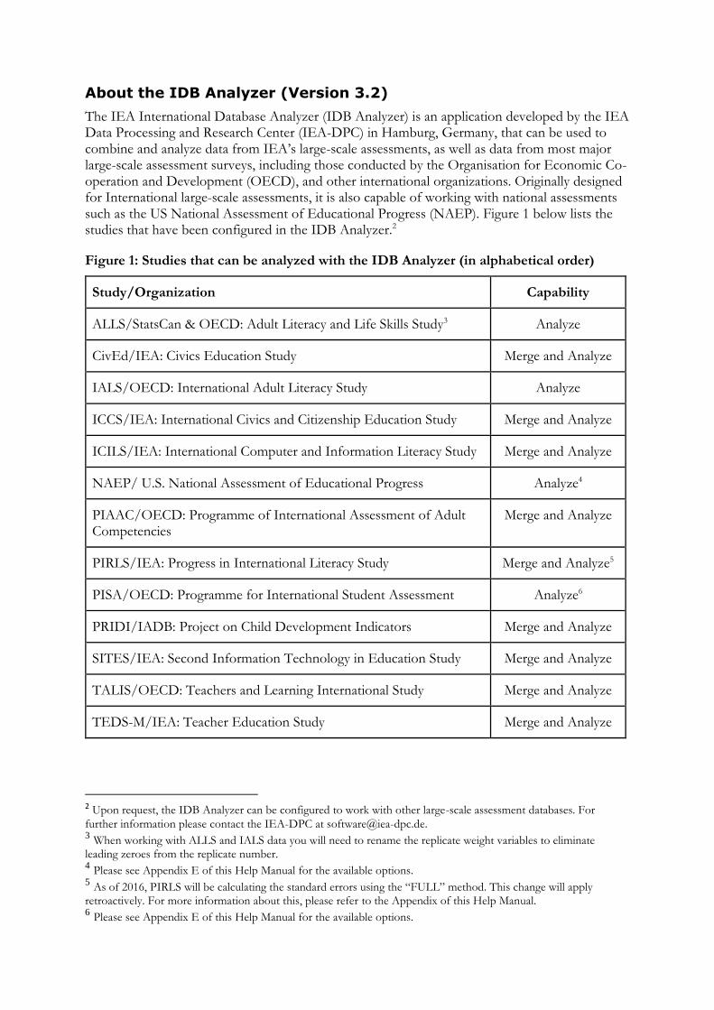
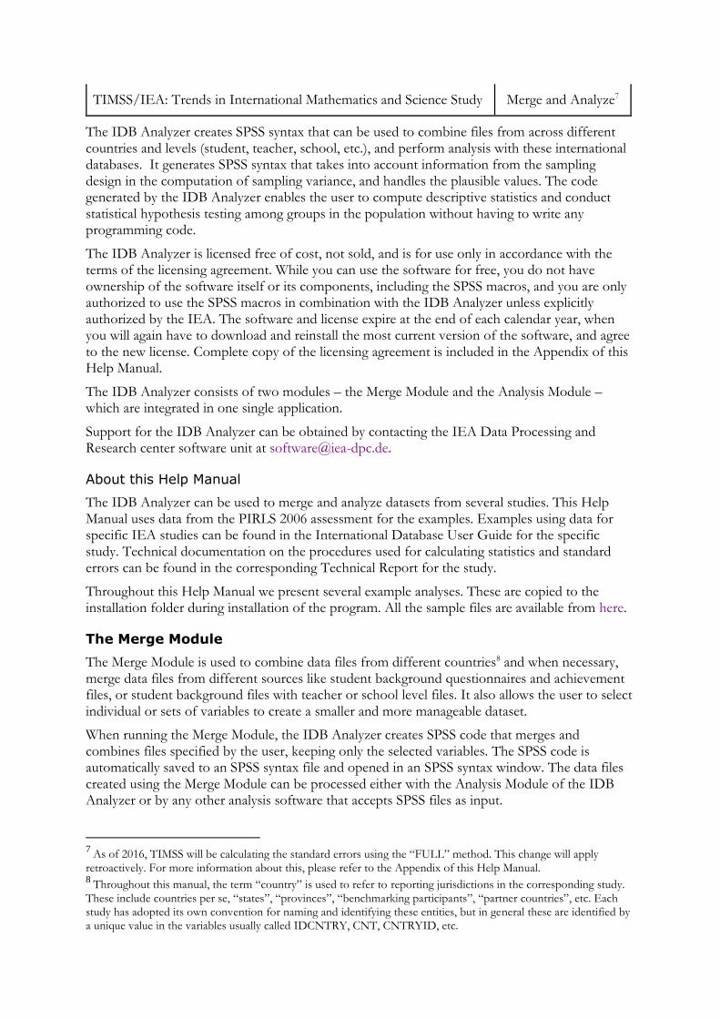
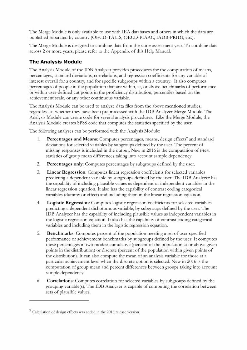


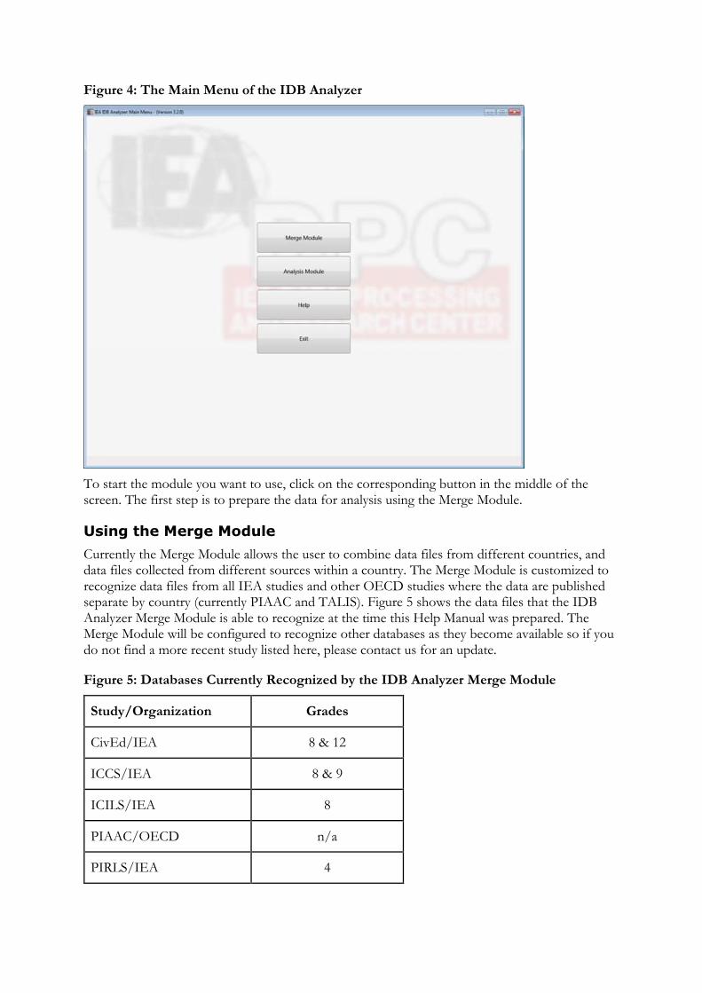
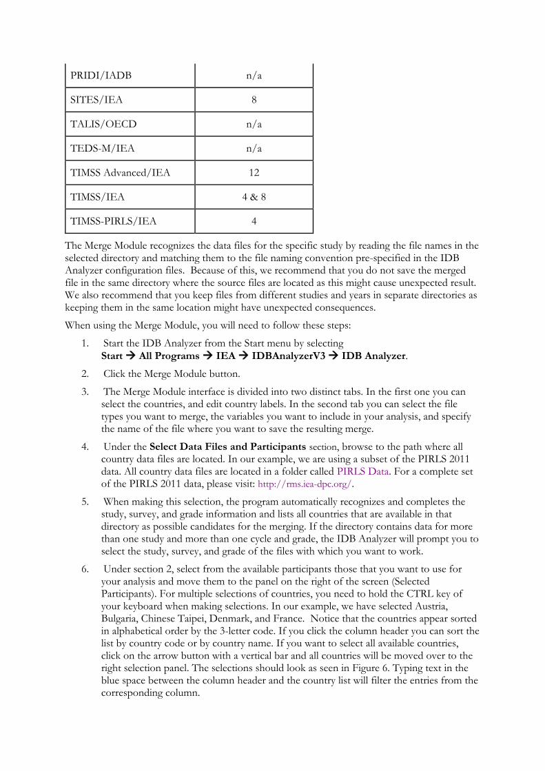

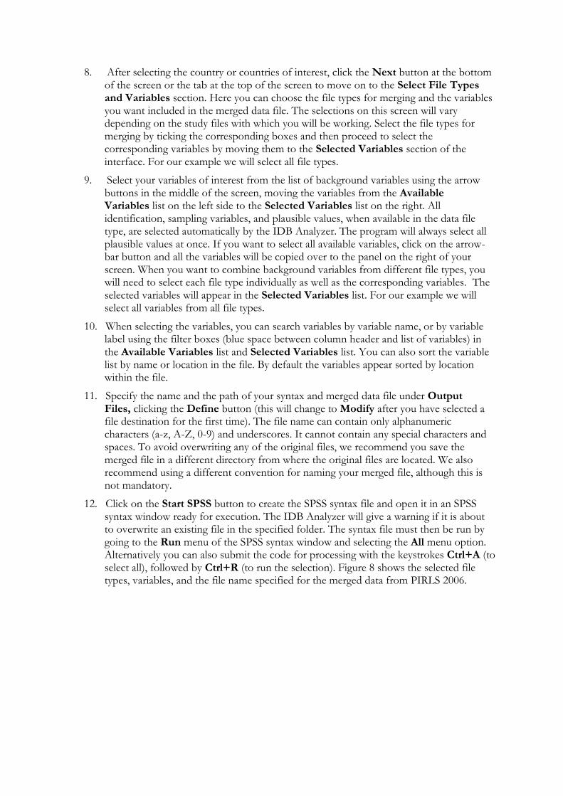
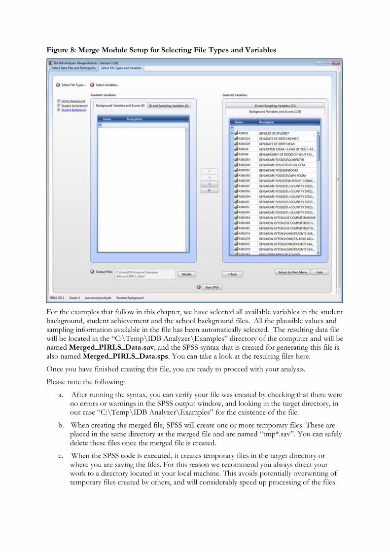
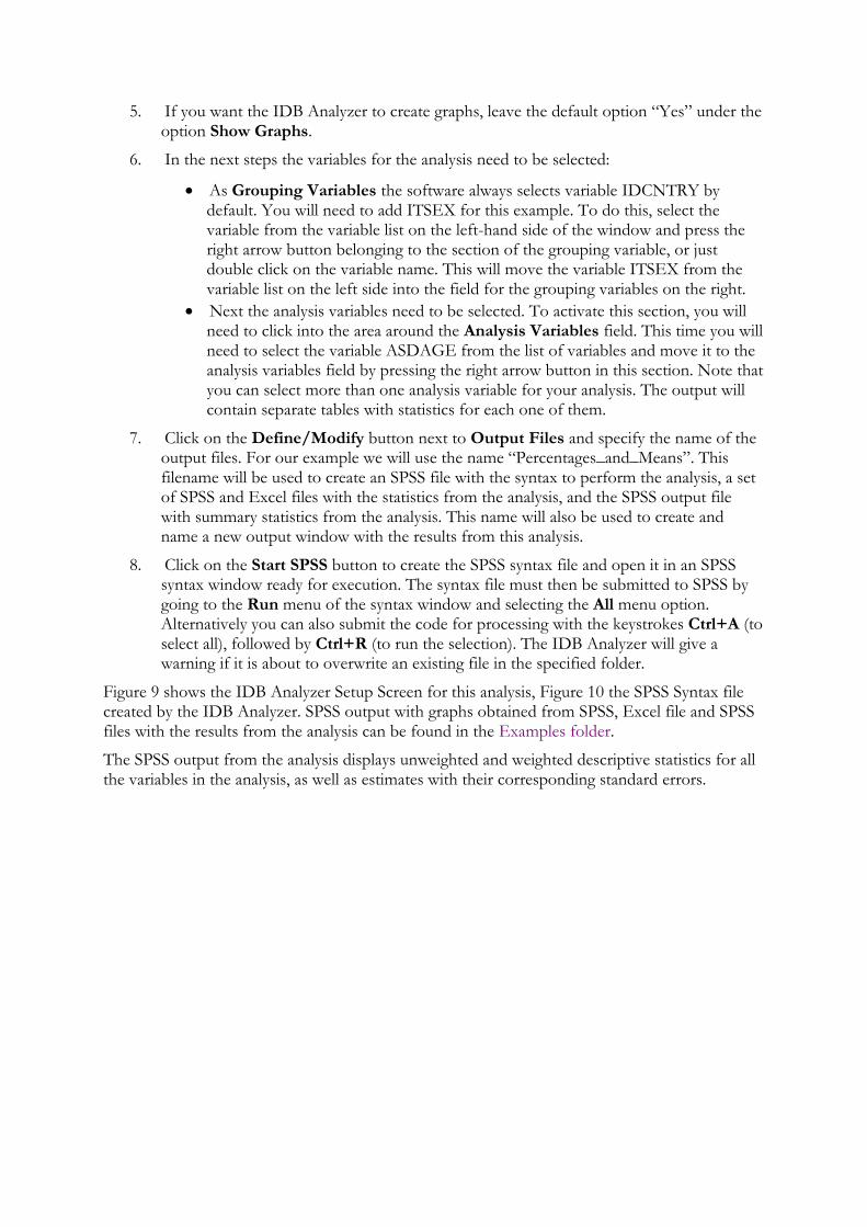
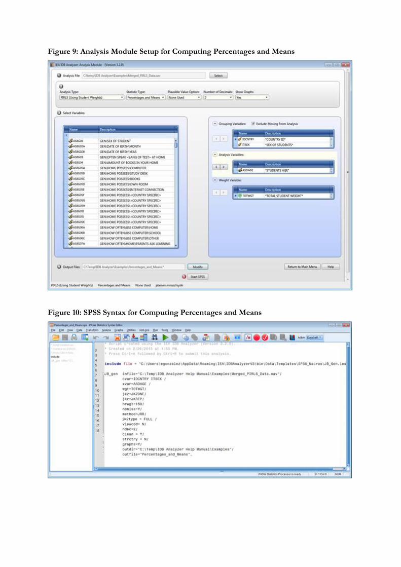
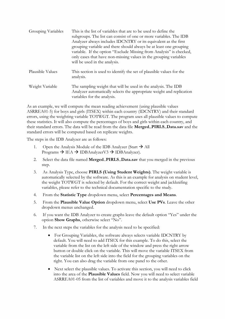

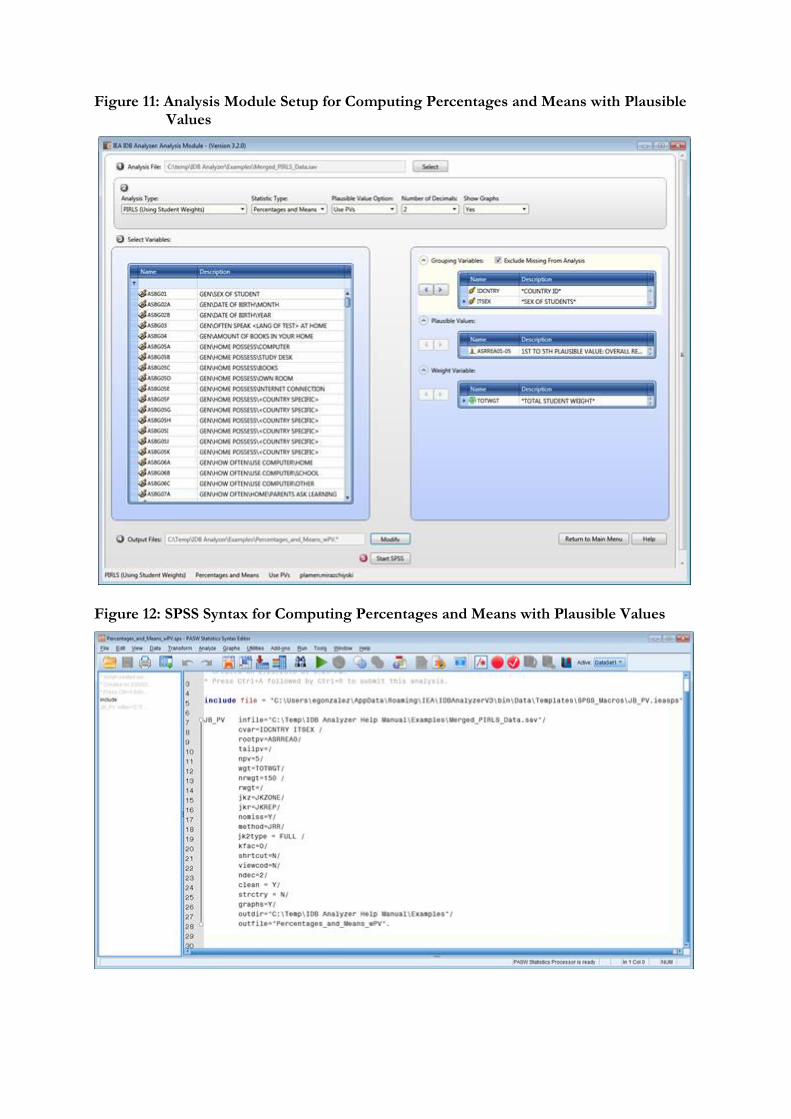
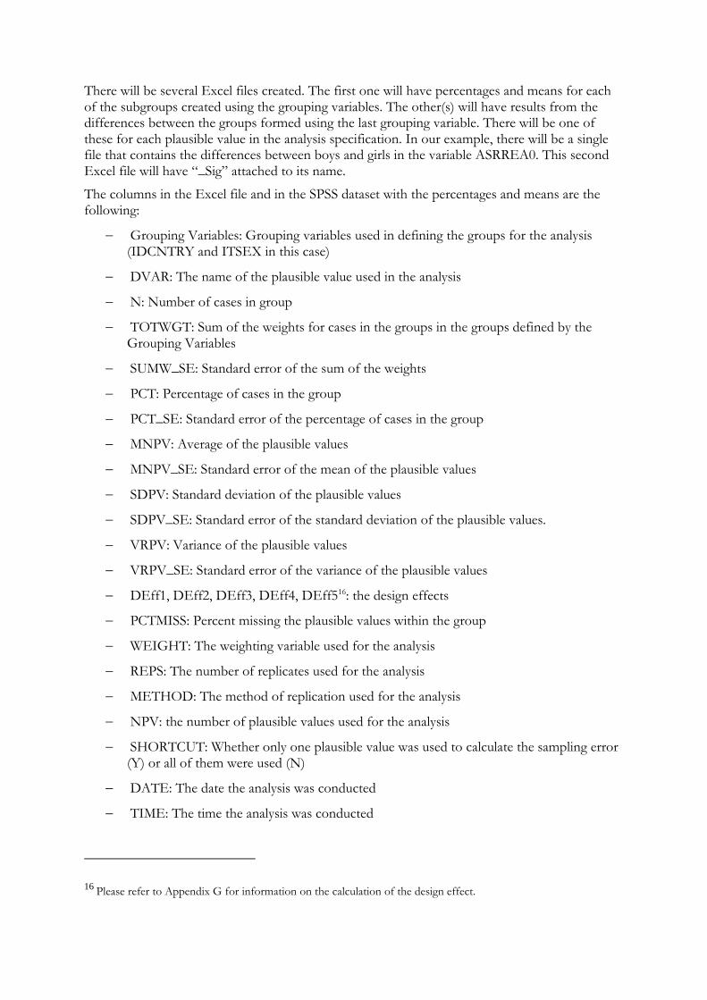


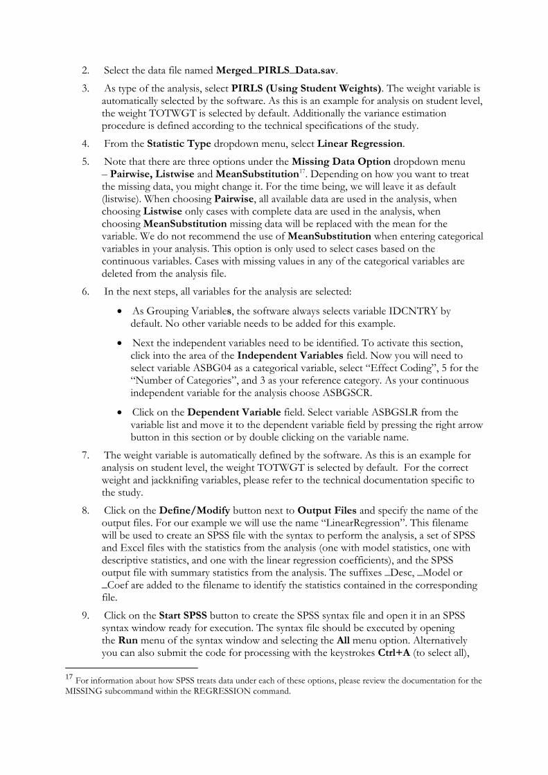
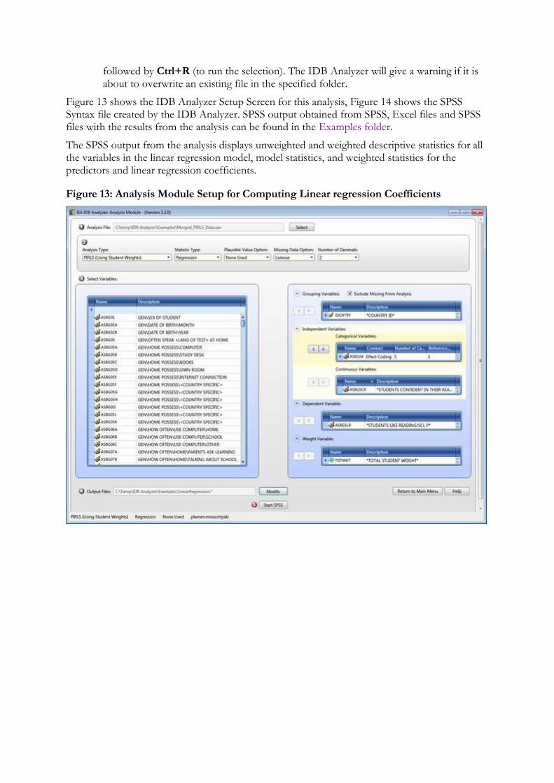

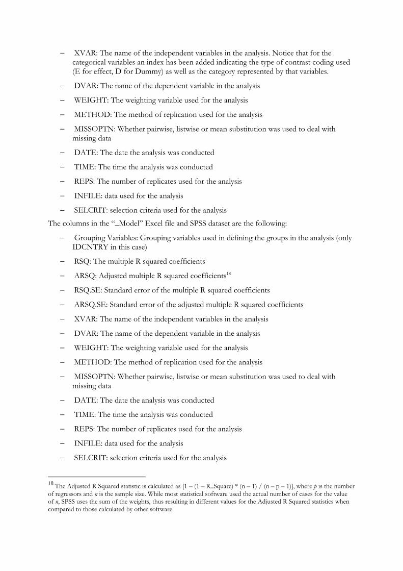


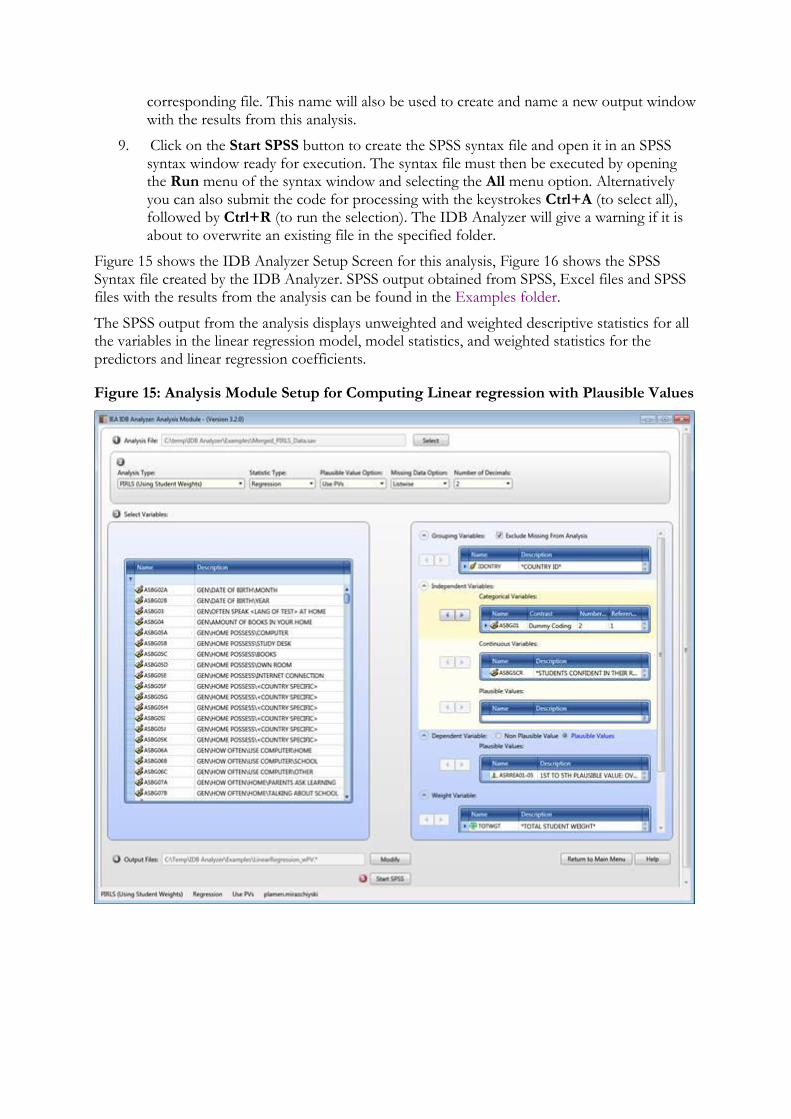

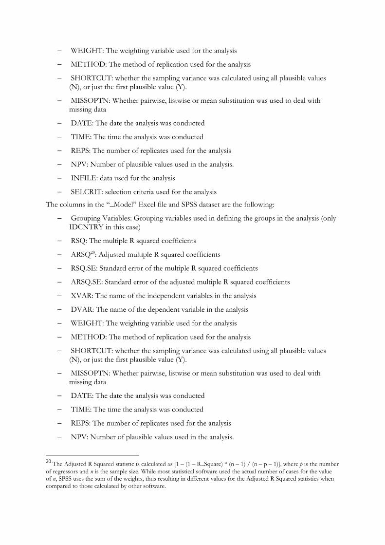

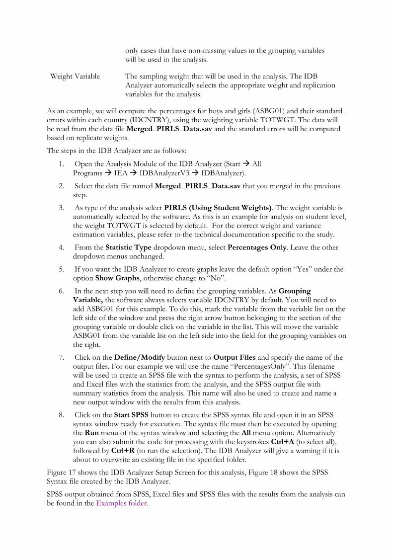
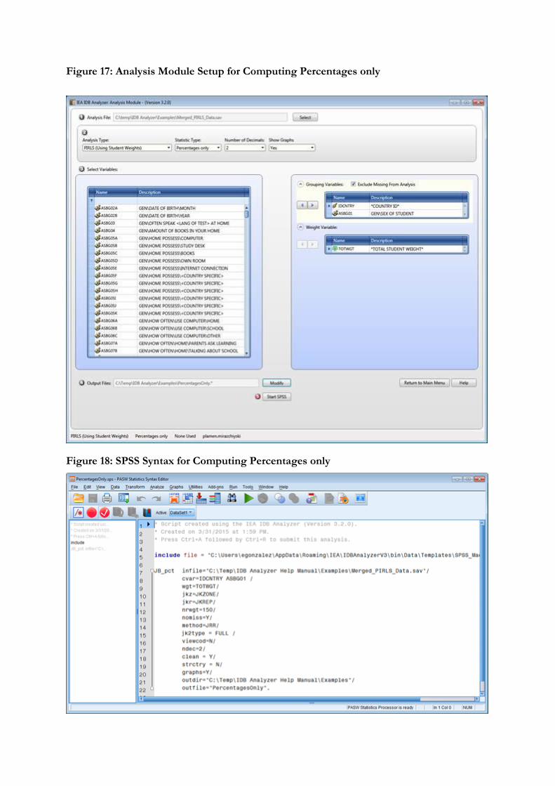
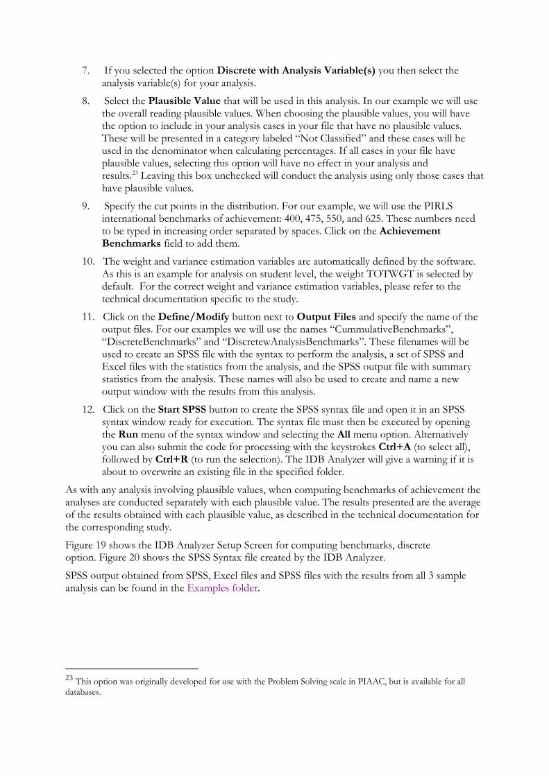
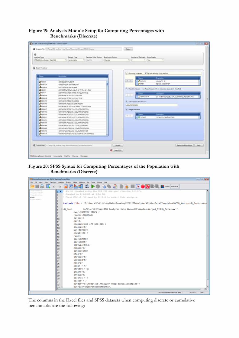


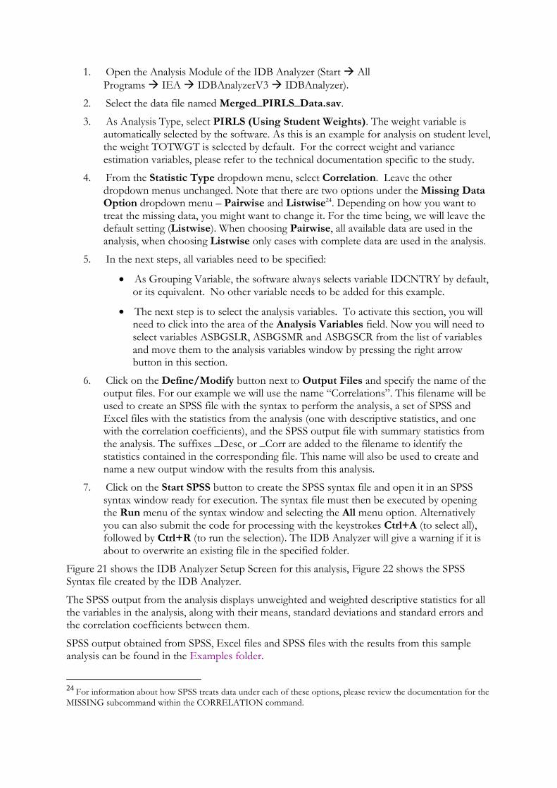
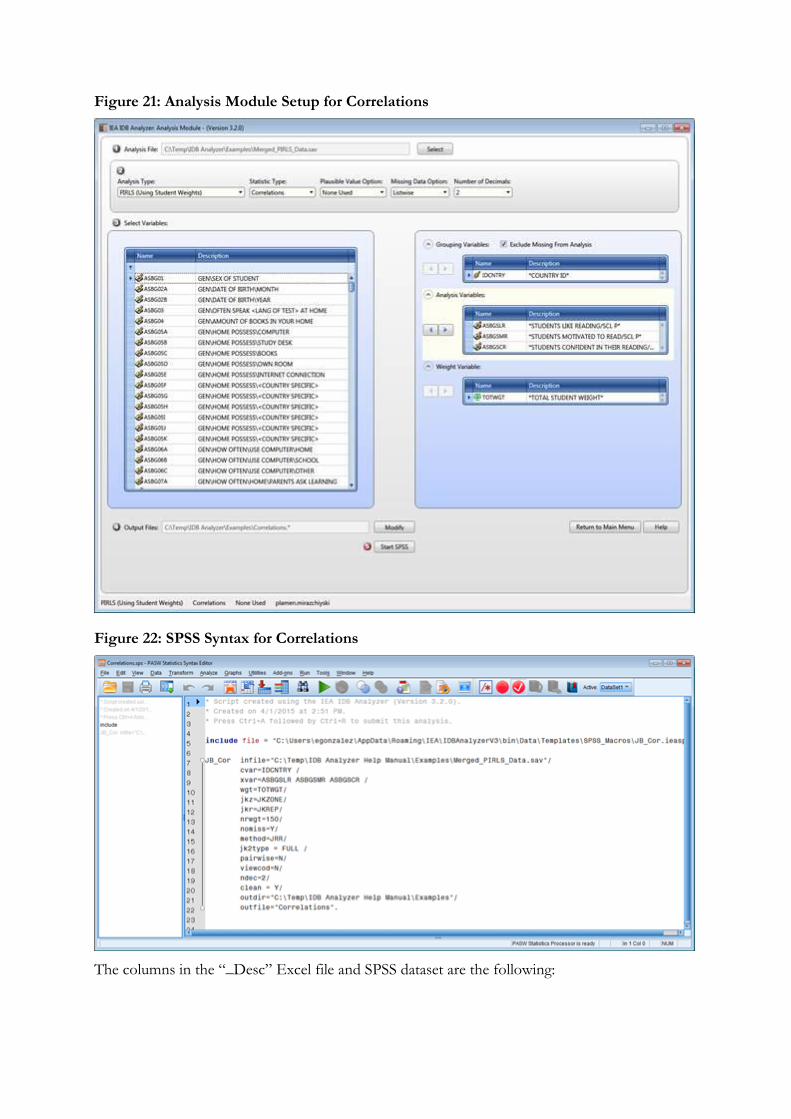


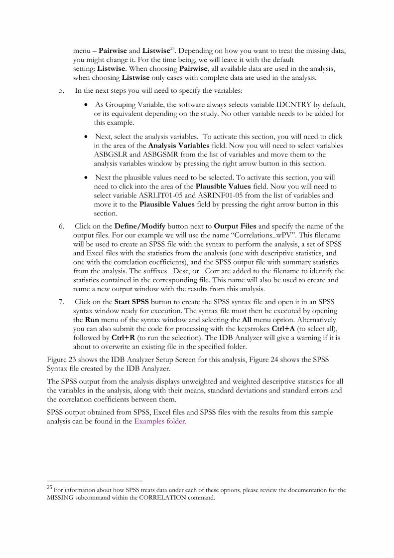
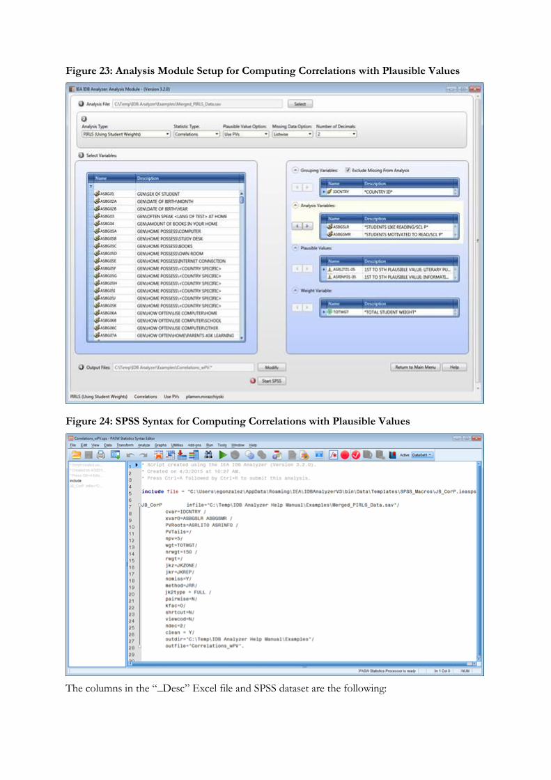
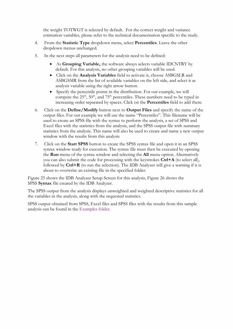
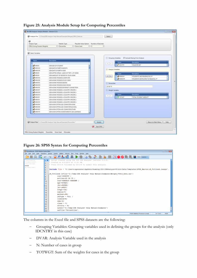
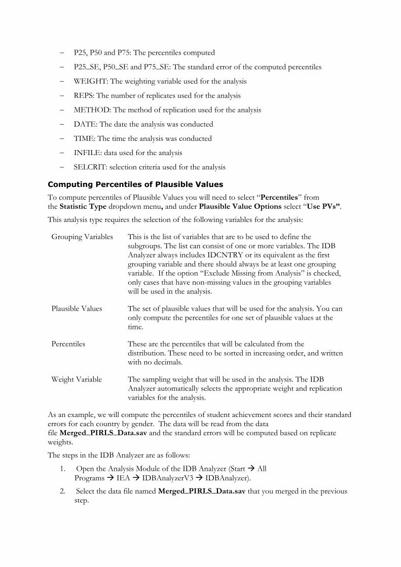
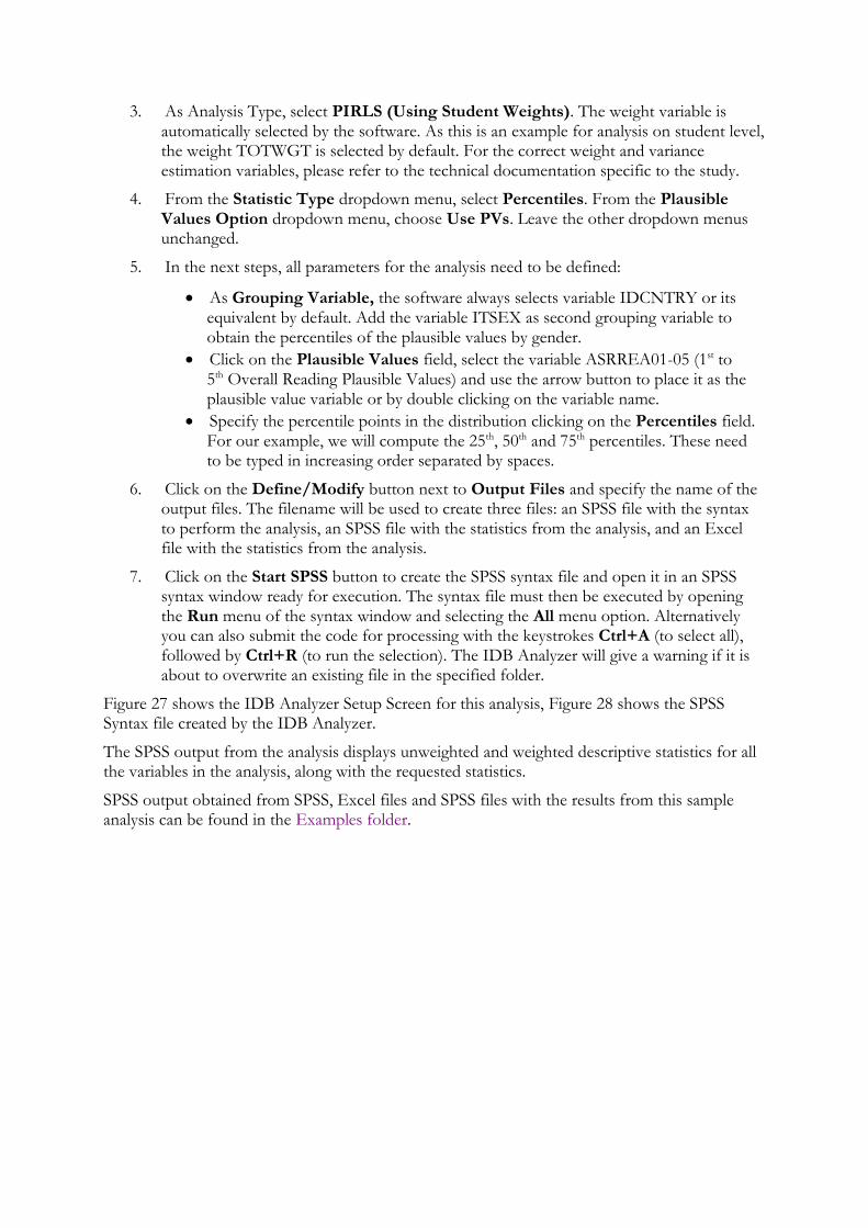
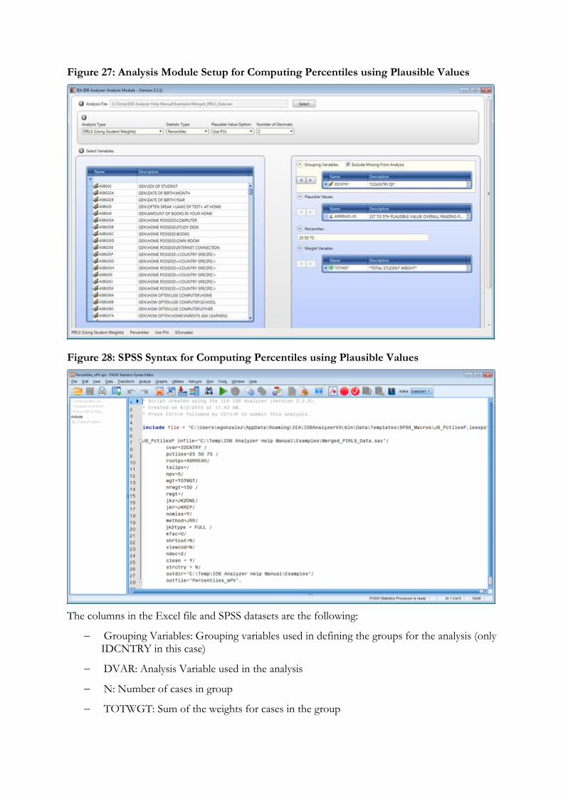

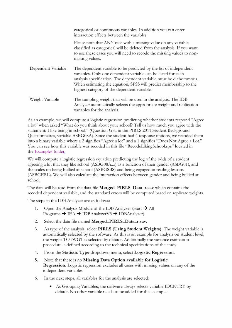


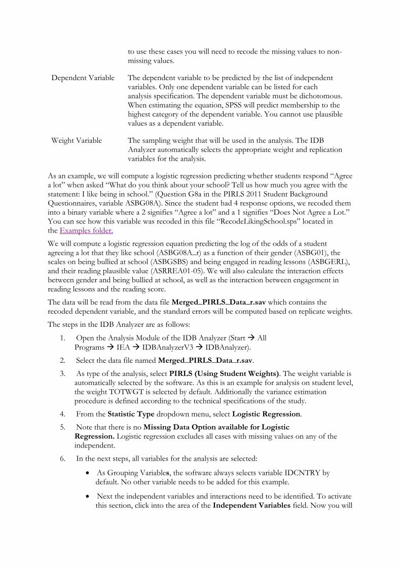

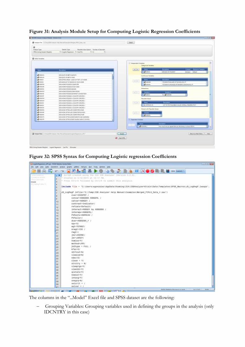
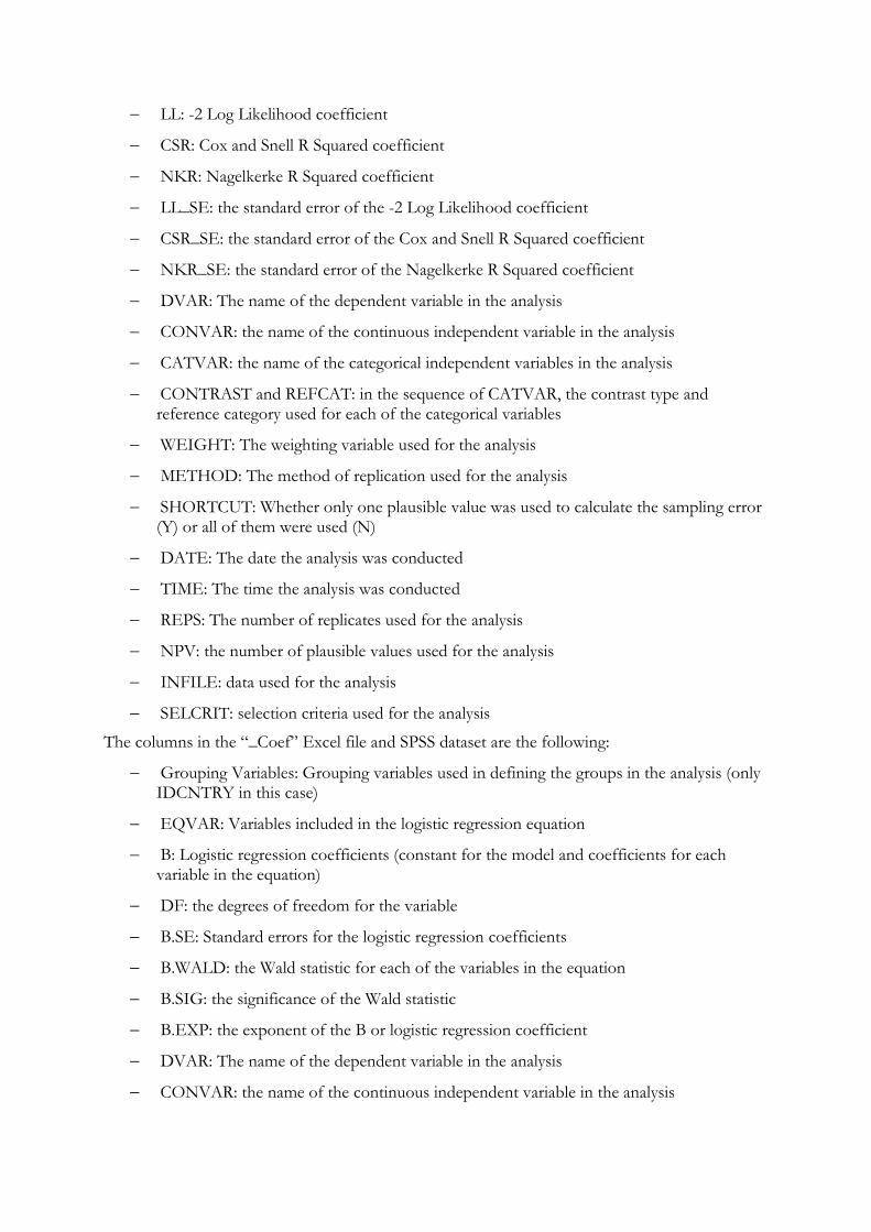
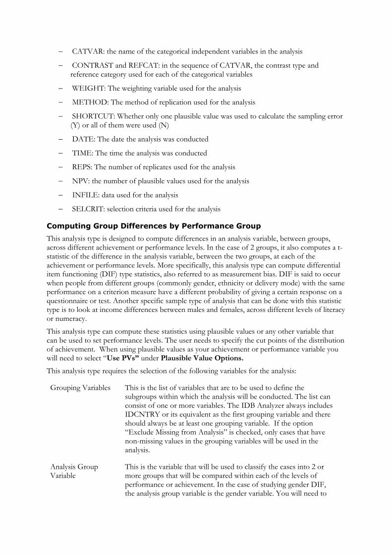
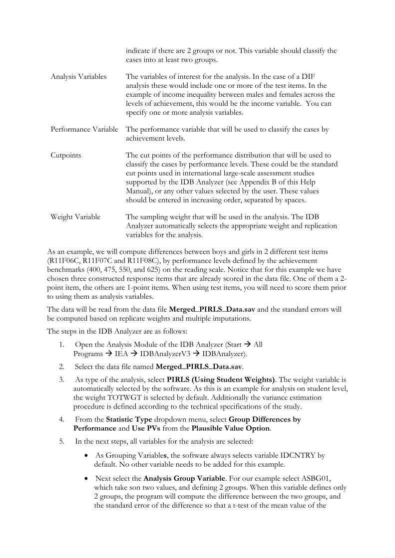

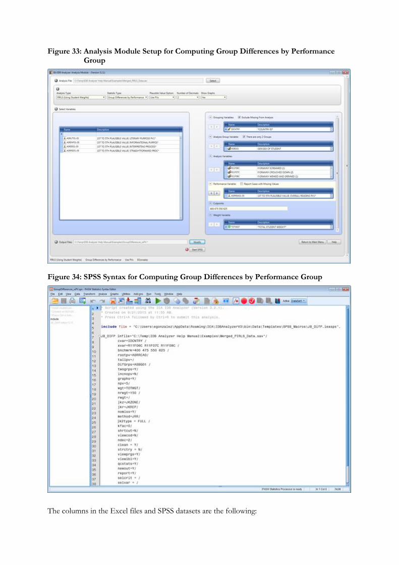
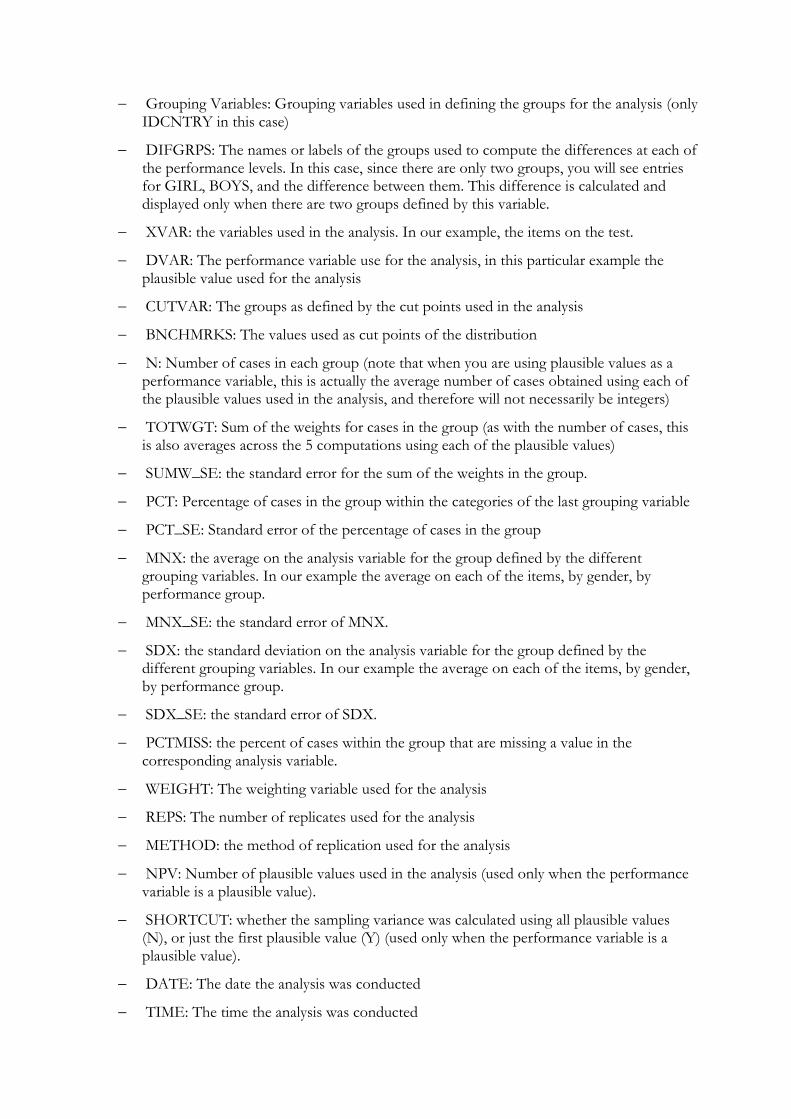
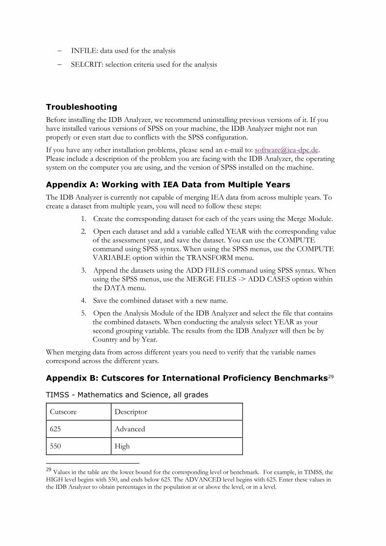
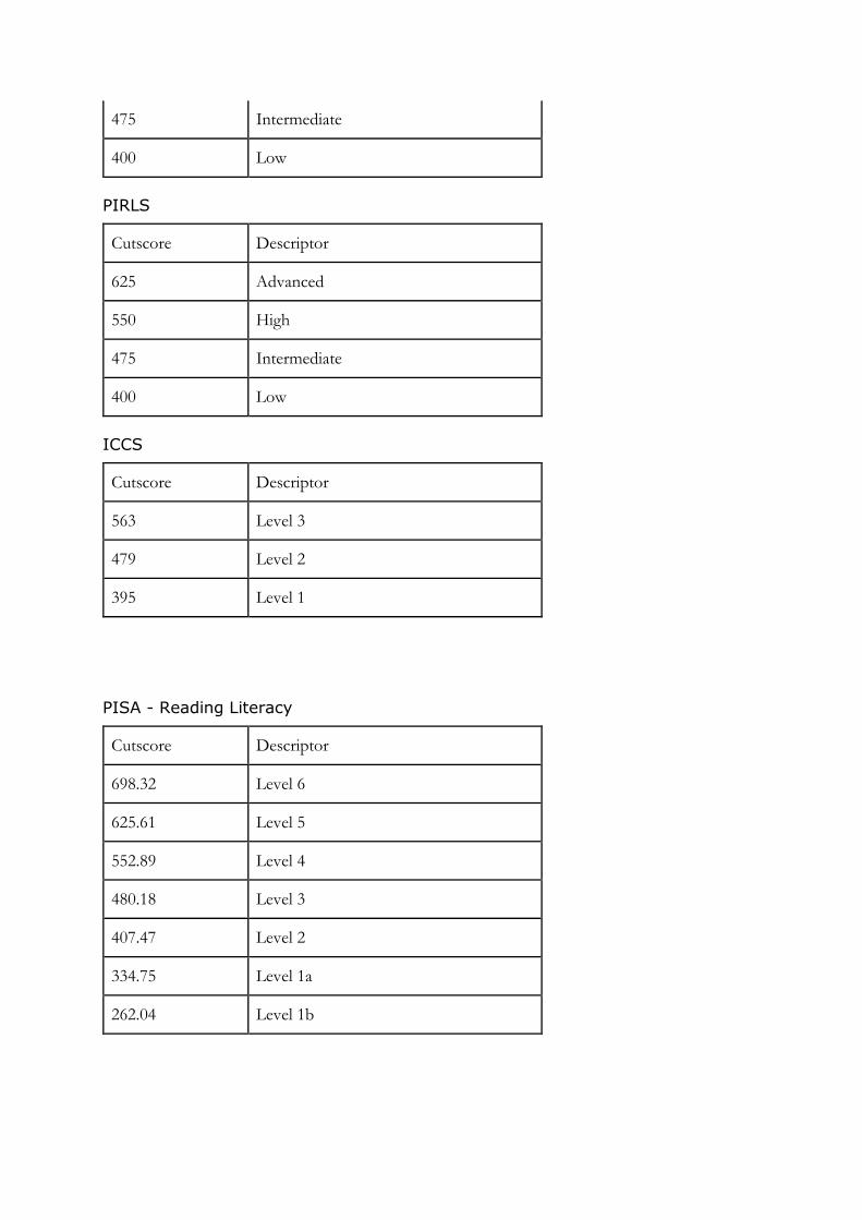
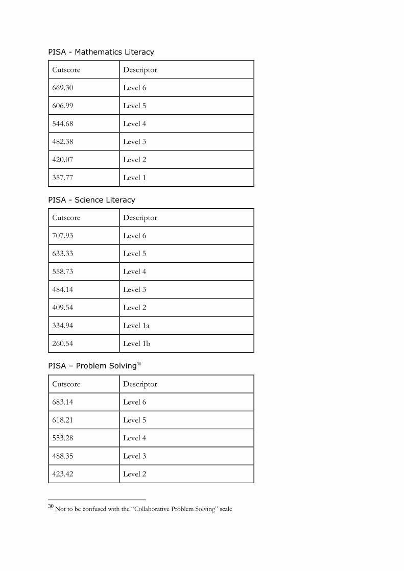
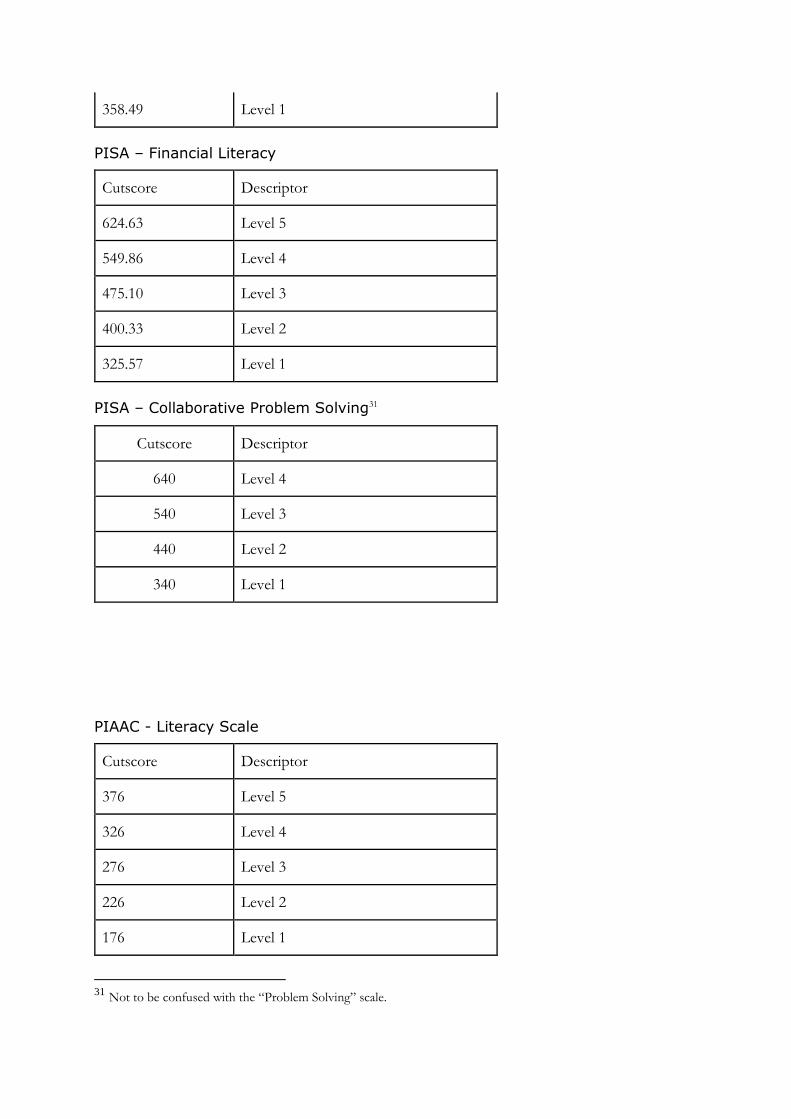
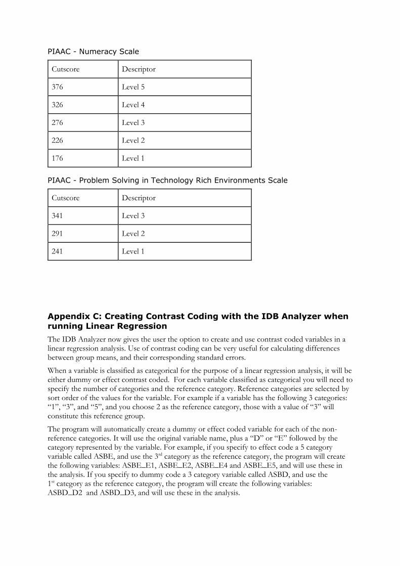

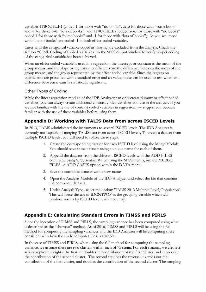
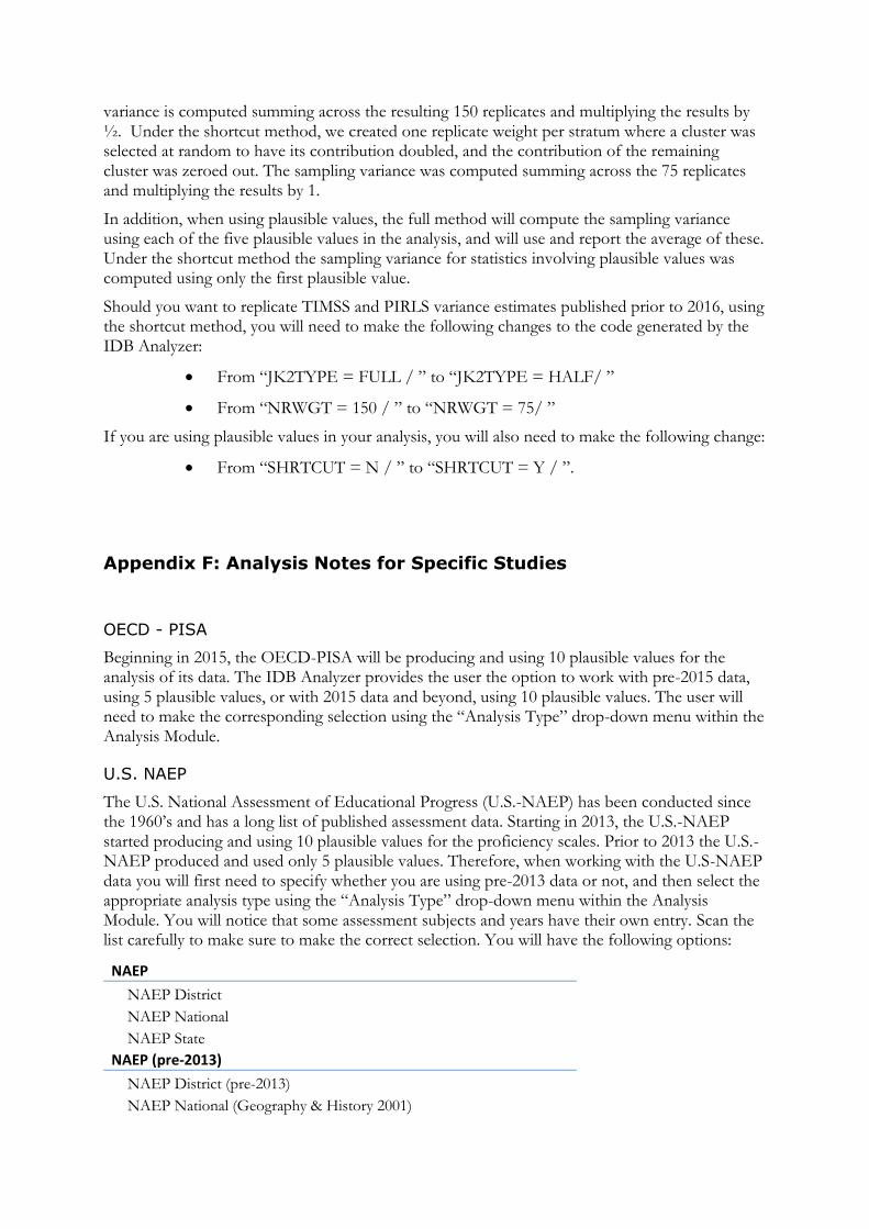

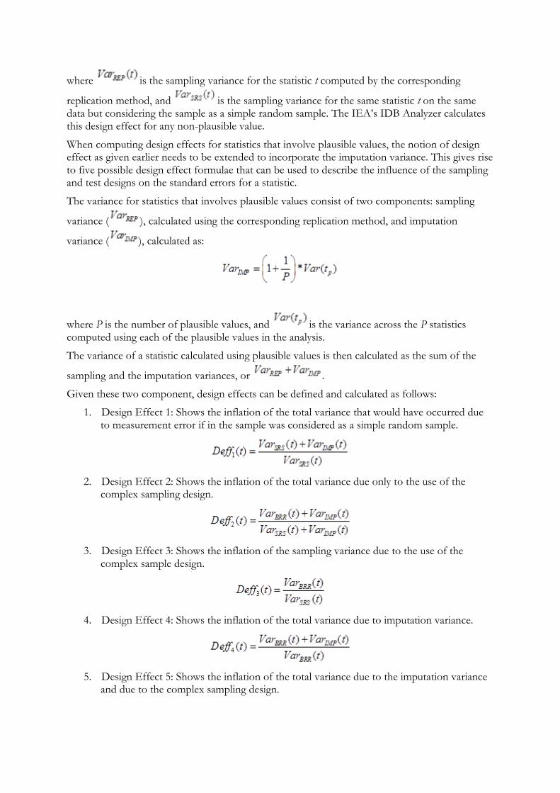


![Presentation idb[1]](https://static.documents.pub/doc/80x56/5477df3db4af9f54028b48b8/presentation-idb1.jpg)


