126
Lecture Note Sketches Spectral Methods for Partial Differential Equations Hermann Riecke Engineering Sciences and Applied Mathematics [email protected] June 3, 2009 1

Lecture Note Sketches
Spectral Methods for Partial Differential Equations
Hermann Riecke
Engineering Sciences and Applied Mathematics
June 3, 2009
1

Contents
1 Motivation and Introduction 8
1.1 Review of Linear Algebra . . . . . . . . . . . . . . . . . . . . . . . . . . . . . . . 9
2 Approximation of Functions by Fourier Series 12
2.1 Convergence of Spectral Projection . . . . . . . . . . . . . . . . . . . . . . . . . 14
2.2 The Gibbs Phenomenon . . . . . . . . . . . . . . . . . . . . . . . . . . . . . . . 22
2.3 Discrete Fourier Transformation . . . . . . . . . . . . . . . . . . . . . . . . . . 25
2.3.1 Aliasing . . . . . . . . . . . . . . . . . . . . . . . . . . . . . . . . . . . . . 29
2.3.2 Differentiation . . . . . . . . . . . . . . . . . . . . . . . . . . . . . . . . . 31
3 Fourier Methods for PDE: Continuous Time 34
3.1 Pseudo-spectral Method . . . . . . . . . . . . . . . . . . . . . . . . . . . . . . . 34
3.2 Galerkin Method . . . . . . . . . . . . . . . . . . . . . . . . . . . . . . . . . . . 36
4 Temporal Discretization 38
4.1 Review of Stability . . . . . . . . . . . . . . . . . . . . . . . . . . . . . . . . . . 39
4.2 Adams-Bashforth Methods . . . . . . . . . . . . . . . . . . . . . . . . . . . . . . 40
4.3 Adams-Moulton-Methods . . . . . . . . . . . . . . . . . . . . . . . . . . . . . . . 43
4.4 Semi-Implicit Schemes . . . . . . . . . . . . . . . . . . . . . . . . . . . . . . . . 46
4.5 Runge-Kutta Methods . . . . . . . . . . . . . . . . . . . . . . . . . . . . . . . . 46
4.6 Operator Splitting . . . . . . . . . . . . . . . . . . . . . . . . . . . . . . . . . . . 49
4.7 Exponential Time Differencing and Integrating Factor Scheme . . . . . . . . 50
4.8 Filtering . . . . . . . . . . . . . . . . . . . . . . . . . . . . . . . . . . . . . . . . 53
5 Chebyshev Polynomials 58
5.1 Cosine Series and Chebyshev Expansion . . . . . . . . . . . . . . . . . . . . . . 58
5.2 Chebyshev Expansion . . . . . . . . . . . . . . . . . . . . . . . . . . . . . . . . 60
6 Chebyshev Approximation 64
6.1 Galerkin Approximation . . . . . . . . . . . . . . . . . . . . . . . . . . . . . . . 64
6.2 Pseudo-Spectral Approximation . . . . . . . . . . . . . . . . . . . . . . . . . . . 65
6.2.1 Implementation of Fast Transform . . . . . . . . . . . . . . . . . . . . . 69
6.3 Derivatives . . . . . . . . . . . . . . . . . . . . . . . . . . . . . . . . . . . . . . . 71
6.3.1 Implementation of Pseudospectral Algorithm for Derivatives . . . . . . 74
2

7 Initial-Boundary-Value Problems: Pseudo-spectral Method 77
7.1 Brief Review of Boundary-Value Problems . . . . . . . . . . . . . . . . . . . . . 78
7.1.1 Hyperbolic Problems . . . . . . . . . . . . . . . . . . . . . . . . . . . . . 78
7.1.2 Parabolic Equations . . . . . . . . . . . . . . . . . . . . . . . . . . . . . . 79
7.2 Pseudospectral Implementation . . . . . . . . . . . . . . . . . . . . . . . . . . . 79
7.3 Spectra of Modified Differentiation Matrices . . . . . . . . . . . . . . . . . . . 80
7.3.1 Wave Equation: First Derivative . . . . . . . . . . . . . . . . . . . . . . 81
7.3.2 Diffusion Equation: Second Derivative . . . . . . . . . . . . . . . . . . . 82
7.4 Discussion of Time-Stepping Methods for Chebyshev . . . . . . . . . . . . . . 84
7.4.1 Adams-Bashforth . . . . . . . . . . . . . . . . . . . . . . . . . . . . . . . 84
7.4.2 Adams-Moulton . . . . . . . . . . . . . . . . . . . . . . . . . . . . . . . . 85
7.4.3 Backward-Difference Schemes . . . . . . . . . . . . . . . . . . . . . . . 86
7.4.4 Runge-Kutta . . . . . . . . . . . . . . . . . . . . . . . . . . . . . . . . . . 87
7.4.5 Semi-Implicit Schemes . . . . . . . . . . . . . . . . . . . . . . . . . . . . 87
7.4.6 Exponential Time-Differencing . . . . . . . . . . . . . . . . . . . . . . . 88
8 Initial-Boundary-Value Problems: Galerkin Method 90
8.1 Review Fourier Case . . . . . . . . . . . . . . . . . . . . . . . . . . . . . . . . . 91
8.2 Chebyshev Galerkin . . . . . . . . . . . . . . . . . . . . . . . . . . . . . . . . . 91
8.2.1 Modification of Set of Basis Functions . . . . . . . . . . . . . . . . . . . 92
8.2.2 Chebyshev Tau-Method . . . . . . . . . . . . . . . . . . . . . . . . . . . 93
9 Iterative Methods for Implicit Schemes 96
9.1 Simple Iteration . . . . . . . . . . . . . . . . . . . . . . . . . . . . . . . . . . . . 96
9.2 Richardson Iteration . . . . . . . . . . . . . . . . . . . . . . . . . . . . . . . . . 98
9.3 Preconditioning . . . . . . . . . . . . . . . . . . . . . . . . . . . . . . . . . . . . 99
9.3.1 Periodic Boundary Conditions: Fourier . . . . . . . . . . . . . . . . . . . 100
9.3.2 Non-Periodic Boundary Conditions: Chebyshev . . . . . . . . . . . . . . 102
9.3.3 First Derivative . . . . . . . . . . . . . . . . . . . . . . . . . . . . . . . . 103
10 Spectral Methods and Sturm-Liouville Problems 105
11 Spectral Methods for Incompressible Fluid Dynamics 109
11.1 Coupled Method . . . . . . . . . . . . . . . . . . . . . . . . . . . . . . . . . . . . 111
11.2 Operator-Splitting Methods . . . . . . . . . . . . . . . . . . . . . . . . . . . . . 113
3

A Insertion: Testing of Codes 117
B Details on Integrating Factor Scheme IFRK4 117
C Chebyshev Example: Directional Sensing in Chemotaxis 120
D Background for Homework: Transitions in Reaction-Diffusion Systems 121
E Background for Homework: Pulsating Combustion Fronts 124
4
Index
2/3-rule, 56
absolute stability, 39
absolutely stable, 39
Adams-Bashforth, 40, 45
Adams-Moulton, 43, 45
adaptive grid, 57
aliasing, 29, 38, 54, 69
Arrhenius law, 26
basis, 11
bounded variation, 15
Brillouin zone, 29
Burgers equation, 36, 37
Cauchy-Schwarz, 19
Chebyshev Expansion, 60
Chebyshev Polynomials, 61
Chebyshev round-off error, 77
chemotaxis, 120
cluster, 62
CNAB, 53, 118
Complete, 13
Completeness, 13
completeness, 12
continuous, 17
Convergence Rate, 19
cosine series, 59
Crank-Nicholson, 44, 121
Decay Rate, 18
diagonalization, 40
differentiation matrix, 77
Diffusion equation, 35
diffusive scaling, 42
discontinuities, 17
effective exponent, 21
exponential time differencing scheme, 51
FFT, 69, 75
Filtering, 53
Fourier interpolant, 29
Gauss-Lobatto integration, 67
Gibbs, 36
Gibbs Oscillations, 57
Gibbs Phenomenon, 22
Gibbs phenomenon, 59
global, 8
Heun’s method, 47
hyperbolic, 39
Improved Euler method, 47
infinite-order accuracy, 20
integrating-factor scheme, 50
integration by parts, 18
interpolates, 40
interpolation, 43
Interpolation error, 30
Interpolation property, 28
Lagrange polynomial, 76
linear transformation, 11
Matrix multiplication method, 32
matrix-multiply, 75
membrane, 120
Method, 34
modified Euler, 47
natural ordering, 71
Neumann stability, 39
Newton iteration, 121
Newton method, 38
non-uniform convergence, 16
normal, 40
numerical artifacts, 57
Operator Splitting, 49
operator splitting error, 49
Orszag, 56
Orthogonal, 13
overshoot, 25
pad, 56
parabolic, 39
Parseval identity, 14
piecewise continuous, 22
pinning, 38
pointwise, 25
5

predictor-corrector, 45
projection, 11, 13
projection error, 30
projection integral, 65
recursion, 71
recursion relation, 61
Runge-Kutta, 46
scalar product, 10
Schwartz inequality, 10, 14
Semi-Implicit, 46
semi-implicit, 121
shock, 53
shocks, 36
Simpson’s rule, 48
singularity, 18
smoothing, 57
Spectral Accuracy, 20
spectral accuracy, 26, 65
Spectral Approximation, 20
spectral blocking, 54
spectral projection, 13, 15
stable, 39
stages, 47
strip of analyticity, 20
Sturm-Liouville problem, 63
total variation, 15
Transform method, 31
trapezoidal rule, 26, 66
turbulence, 53
two-dimensionsional, 45
unconditionally stable, 44
unique, 47
Variable coefficients, 35
variable wave speed, 45
Variable-coefficient, 37
vector space, 10
weight, 62
weighted scalar product, 62
6

References
[1] C. Canuto, M. Y. Hussaini, A. Quarteroni, and T. A. Zang. Spectral methods in fluid
dynamics. Springer, 1987.
[2] C. Canuto, M. Y. Hussaini, A. Quarteroni, and T. A. Zang. Spectral methods: funda-
mentals in single domains. Springer, 2006.
[3] C. Canuto, M. Y. Hussaini, A. Quarteroni, and T. A. Zang. Spectral methods: evolution
to complex geometries and applications to fluid dynamics. Springer, 2007.
[4] M. Charalambides and F. Waleffe. Gegenbauer tau methods with and without spurious
eigenvalues. SIAM J. Num. Anal., 47(1):48–68, 2008.
[5] D. Gottlieb and S. A. Orszag. Numerical Analysis of Spectral Methods: Theory and
Applications. 1977.
[6] R. A. Horn and C. R. Johnson. Topics in matrix analysis. Cambridge University Press,
1994.
[7] A.-K. Kassam and L. N. Trefethen. Fourth-order time-stepping for stiff pdes. SIAM J.
Sci. Comput., 26:1214, 2005.
[8] B. J. Matkowsky and D. O. Olagunju. Propagation of a pulsating flame front in a
gaseous combustible mixture. SIAM J. Appl. Math., 39(2):290–300, 1980.
[9] A. Palacios, G. H. Gunaratne, M. Gorman, and K. A. Robbins. Cellular pattern forma-
tion in circular domains. Chaos, 7(3):463–475, September 1997.
7

1 Motivation and Introduction
Central step when solving partial differential equations: approximate derivatives in space
and time. Focus here on spatial derivatives.
Finite difference approximation of (spatial) derivatives:
• Accuracy depends on order of approximation ⇒ number of grid points involved in the
computation (width of ‘stencil’)
• For higher accuracy use higher-order approximation
⇒ use more points to calculate derivatives
• function is approximated locally by polynomials of increasing order
To get maximal order use all points in system
⇒ approximate function globally by polynomials
More generally:
• approximate function by suitable global functions fk(x)
u(x) =
∞∑
k=1
ukfk(x)
fk(x) need not be polynomials
• calculate derivative of fk(x) analytically: exact⇒ error completely in expansion
Notes:
• For smooth functions the order of the approximation of the derivative is higher than
any power.
• high derivatives not problematic
8

a) b)
Figure 1: a) finite differences: local approximation u = u1, u2, ...uN . Unknowns: values at
grid points. b) spectral: global approximation . Unknowns: Fourier amplitudes
Note: in pseudo-spectral methods again values at grid points used although expanded in a
set of global functions
Thus:
• Study approximation of functions by sets of other functions
• Impact of spectral approach on treatment of temporal evolution
We will use Fourier modes and Chebyshev polynomials.
Recommended books (for reference)
• Spectral Methods by C. Canuto, M.Y. Hussaini, A. Quarteroni, and T.A. Zang, Springer.
They have written three books. [1, 2, 3]. The two new ones are not expensive.
• Spectral Methods in MATLAB by L.N. Trefethen, SIAM, ISBN 0898714656. Not ex-
pensive.
• Chebyshev and Fourier Spectral Methods by J.P. Boyd, Dover (2001). Available online
at http://www-personal.umich.edu/~jpboyd/BOOK_Spectral2000.html and
is also not expensive to buy.
1.1 Review of Linear Algebra
Motivation: Functions can be considered as vectors
=⇒ consider approximation of vectors by other vectors
9

Definition: V is a real (complex) vector space if for all u,v ∈ V and all α, β ∈ R(C)
αu + βv ∈ V
Examples:
a) R3 = {(x, y, z)|x, y, z ∈ R} is a real vector space
b) Cn is a complex vector space
c) all continuous functions form a vector space:
αf(x) + βg(x) is a continuous function if f(x) and g(x) are
d) The space V = {f(x)|continuous, 0 ≤ x ≤ L, f(0) = a, f(L) = b} is only a vector space for
a = 0 = b. Why?
Definition: For a vector space V < ·, · >: V × V → C is called a scalar product or inner
product iff
< u, v > = < v, u >∗
< αu+ βv, w > = α∗ < u,w > +β∗ < v,w >, α, β ∈ C
< u, u > ≥ 0
< u, u >= 0 ⇔ u = 0.
Notes:
• < u, v > is often written as u+ · v with u+ denoting the transpose and complex conju-
gate of u.
• v is a column vector, u+ is a row vector
Examples:
a) in R3: < u, v >=∑3
i=1 uivi is a scalar product
b) in L2 ≡ {f(x)|∫∞−∞ |f(x)|2 dx <∞}
< u, v > =
∫ ∞
−∞u∗(x)v(x) dx
is a scalar product.
Notes:
• u(x) can be considered the “x− th component” of the abstract vector u.
• < u, u >≡ ||u|| defines a norm.
• scalar product satisfies Cauchy-Schwartz inequality
| < u, v > | ≤ ||u|| ||v||
(since the cosine of the angle between the vectors is smaller than 1)
10

Definition: The set {v1, ...,vN} is called an orthonormal complete set (or basis) of V if any
vector u ∈ V can be written as
u =N∑
k=1
ukvk,
with v+i · vj ≡ < vi,vj >= δij.
Calculate the coefficients ui:
< vj ,u >=∑
k
uk < vj ,vk >=∑
k
ukδkj = uj
Example: projections in R2
u1v1 =< v1,u > v1 is the projection of u onto v1.
Projections take one vector and transform it into another vector:
Definition: L : V → V is called a linear transformation iff
L(αv + βw) = αLv + βLw
Definition: A linear transformation P : V → V is called a projection iff
P 2 = P
Examples:
1. Pv = N−1v v+ with N = v+ · v is a projection onto v:
Pvu = vv+ · uv+ · v
P 2v u = v
v+
v+ · v ·(
vv+ · uv+ · v
)
= vv+ · uv+ · v = Pvu
Notes:
11

• v can be thought of as a column vector and v+ a row vector
⇒ v+ · v is a scalar while v v+ is a projection operator
• v+ · u/v+ · v is the length of the projection of u onto v
2. Let {vi, i = 1..N} be a complete orthonormal set
u =N∑
k=1
(v+k · u)vk = (
N∑
k=1
vkv+k ) · u
thus we haveN∑
k=1
vkv+k = I
i.e. the sum over all projections onto a complete set yields the identity transformation:
completeness of the set v
3. A linear transformation L can be represented by a matrix:
(Lu)i = v+i L
N∑
j=1
ujvj =∑
j
v+i Lvj uj =
∑
j
Lijuj
with
Lij = v+i Lvj
The identity transformation is given by the matrix
Iij = v+i (∑
k
vkv+k )vj =
∑
k
δikδkj = δij
can write this also as
Iij =∑
k
v+i vk︸ ︷︷ ︸
ith−component of vk
·(v+
j vk
)+
︸ ︷︷ ︸
cc of jth−component of vk
(1)
Note: The matrix elements Lij depend on the choice of the basis
Getting back to functions: Vector spaces formed by functions often cannot be spanned by
a finite number of vectors, i.e. no finite set {v1, ...,vN} suffices ⇒ need to consider se-
quences and series of vectors. We will not dwell on this sophistication.
2 Approximation of Functions by Fourier Series
Periodic boundary conditions are well suited to study phenomena that are not dominated
by boundaries. For periodic functions it is natural to attempt approximations by Fourier
series.
Consider the set of functions {φk(x) = eikx|k ∈ N}. It forms a complete orthogonal set of
L2[0, 2π].
12

1. Orthogonal
φ+k · φl ≡< φk, φl >=
∫ 2π
0
(eikx)∗eilx dx = 2πδlk
as before eikx is the xth-component of φk
2. Complete:
for any u(x) ∈ L2[0, 2π] there exist {uk|k ∈ N}
limN→∞
||u(x) −N∑
k=−N
ukφk(x)||2 = 0
i.e.
limN→∞
∫ 2π
0
|u(x) −N∑
k=−N
ukeikx|2 dx = 0
with the Fourier components given by
uk =1
2π< φ+
k , u >=1
2π
∫ 2π
0
e−ikxu(x) dx
Note:
• Completeness∑N
k=1 vkv+k = I (cf (1)) implies
limN→∞
∞∑
|k|=0
φk(x)φ+k (x′) = lim
N→∞
N∑
|k|=0
eik(x−x′) = 2π
∞∑
l=−∞δ(x− x′ + 2πl). (2)
Definition: The spectral projection PNu(x) of u(x) is defined as
PNu(x) =
N∑
|k|=0
ukφk(x).
Thus,
limN→∞
||u(x) − PNu(x)||2 = 0.
Notes:
• PN is a projection, i.e. P 2N = PN (see homework)
• PN projects u(x) onto the subspace of the lowest 2N + 1 Fourier modes
13

• ||PNu(x)||2 = 2π∑N
|k|=0 |uk|2:
||PNu(x)||2 = < PNu, PNu >
= <
N∑
|k|=0
ukφk(x),
N∑
|l|=0
ulφl(x) >
=∑
kl
u∗kul < φk(x), φl(x) >
=∑
kl
u∗kul 2π δkl
= 2πN∑
|k|=0
|uk|2.
• Parseval identity extends this to the limit N → ∞ :
•||u||2 = lim
N→∞||PNu||2 = lim
N→∞2π
∞∑
|k|=0
|uk|2
i.e. the L2−norm of a vector is given by the sum of the squares of its components for
any orthonormal complete set. Thus, as more components are included the retained
“energy” approaches the full energy.
Proof: we have
limN→∞
||u(x) − PNu(x)||2 = 0
and want to conclude ||u(x)||2 = limN→∞ ||PNu(x)||2.Consider
(||u|| − ||v||)2 = ||u||2 + ||v||2 − 2||u|| ||v||≤ ||u||2 + ||v|2 − 2| < u, v > |
using Schwartz inequality | < u, v > | ≤ ||u|| ||v|| (projection is smaller than the whole
vector).
Now use 2| < u, v > | ≥ 2Re(< u, v >) =< u, v > + < v, u > (note < u, v > is in general
complex).
Then
||u||2 − ||v||2 ≤ ||u||2 + ||v|2− < u, v > − < v, u >=< u− v, u− v >= ||u− v||2.
Get Parseval identity with v = PNu.
2.1 Convergence of Spectral Projection
Convergence of Fourier series depends strongly on the function to be approximated
14
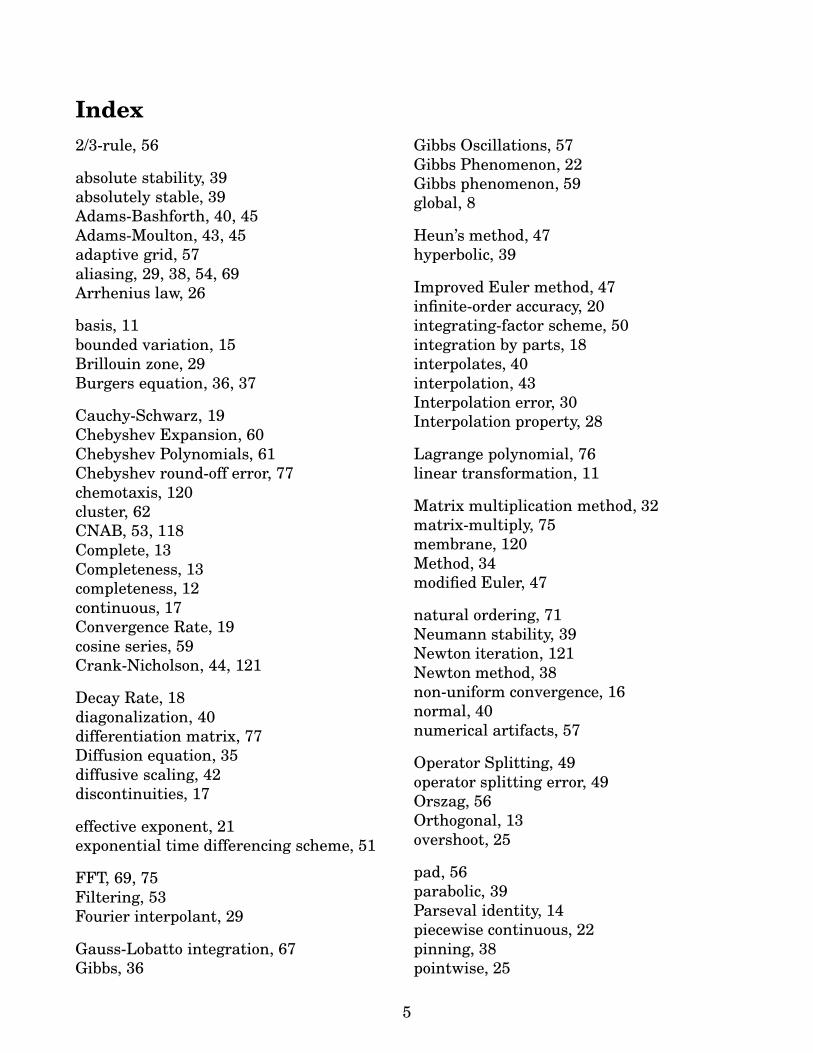
The highest wavenumber needed to approximate a function well surely depends on the
number of “wiggles” of that function.
Definition: The total variation V(u) of a function u(x) on [0, 2π] is defined as
V(u) = supn
sup0=x0<x1<...<xn=2π
n∑
i=1
|u(xi) − u(xi−1)|
Notes:
• the supremum is defined as the lowest upper bound
• for supremum need only consider xi at extrema
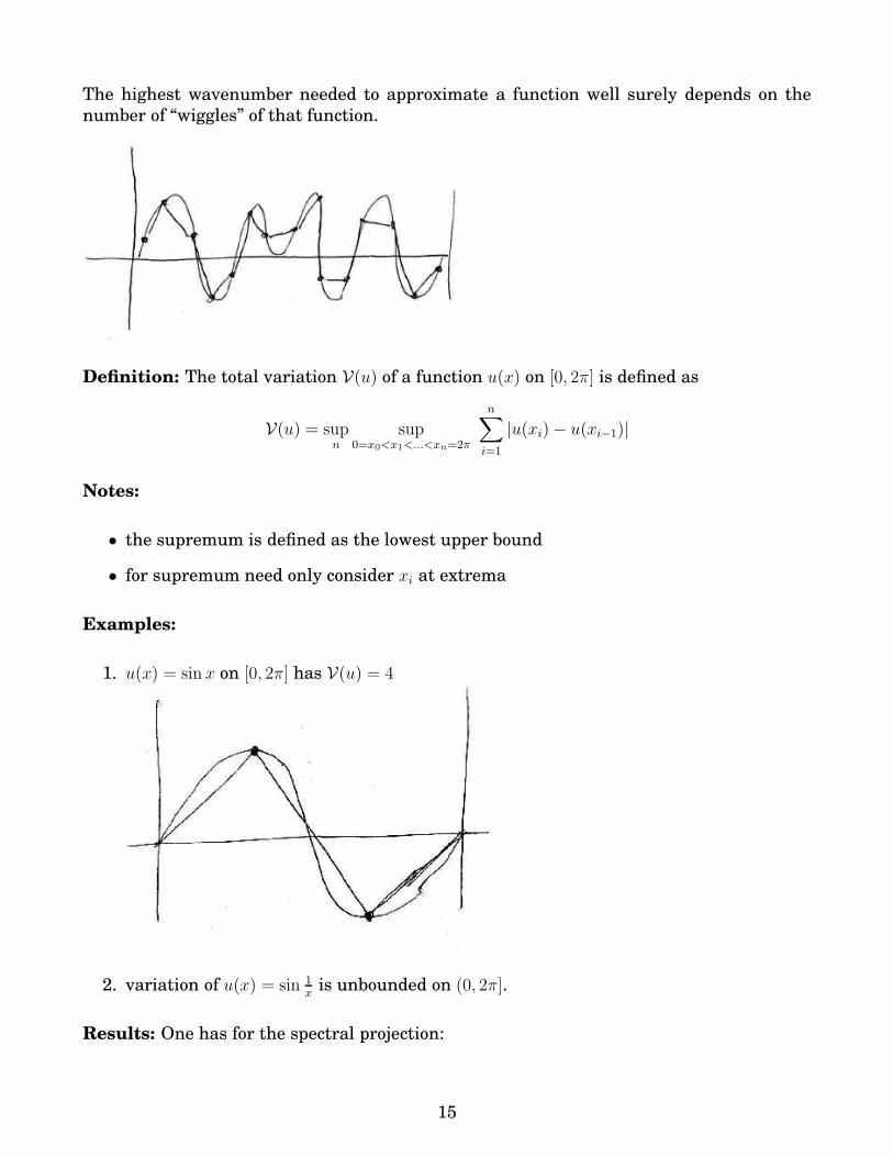
Examples:
1. u(x) = sin x on [0, 2π] has V(u) = 4
2. variation of u(x) = sin 1xis unbounded on (0, 2π].
Results: One has for the spectral projection:
15
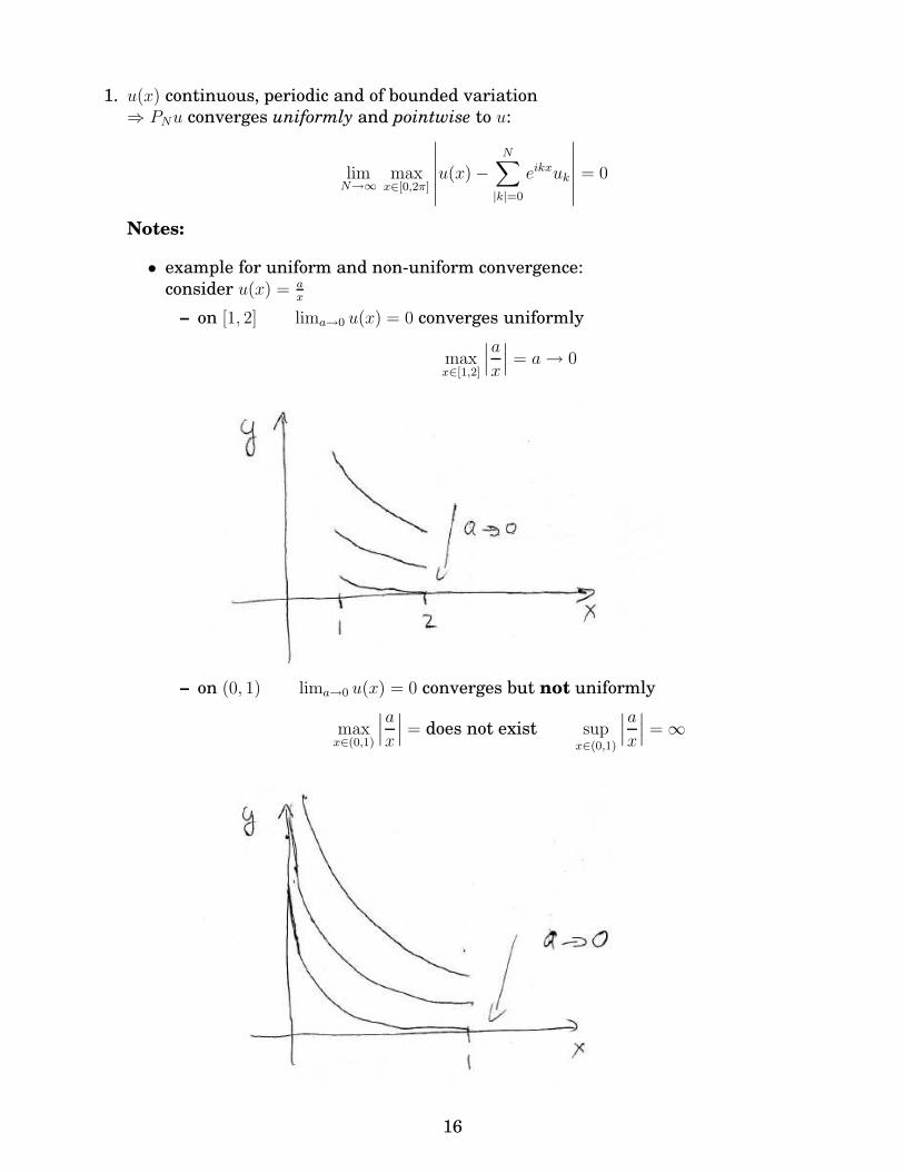
1. u(x) continuous, periodic and of bounded variation
⇒ PNu converges uniformly and pointwise to u:
limN→∞
maxx∈[0,2π]
∣∣∣∣∣∣
u(x) −N∑
|k|=0
eikxuk
∣∣∣∣∣∣
= 0
Notes:
• example for uniform and non-uniform convergence:
consider u(x) = ax
– on [1, 2] lima→0 u(x) = 0 converges uniformly
maxx∈[1,2]
∣∣∣a
x
∣∣∣ = a→ 0
– on (0, 1) lima→0 u(x) = 0 converges but not uniformly
maxx∈(0,1)
∣∣∣a
x
∣∣∣ = does not exist sup
x∈(0,1)
∣∣∣a
x
∣∣∣ = ∞
16

Thus:
uniform convergence of Fourier approximation ⇒ there is an upper bound for error
along the whole function (upper bound on global error).
2. u(x) of bounded variation
⇒ PNu converges pointwise to 12(u+(x) + u−(x)) for any x ∈ [0, 2π] where at discontinu-
ities u±(x) = u(x± ǫ)Note: even if u(x) is discontinuous PNu(x) is always continuous for finite N
(a)
Figure 2: The spectral approximation is continuous even if the function to be approximated
is discontinuous.
3. For u(x) ∈ L2 the projection PNu converges in the mean,
limN→∞
∫ ∞
−∞|u(x) −
∑
k
φkuk|2 dx = 0
but possibly u(x0) 6= PNu(x0) at isolated values of x0, i.e. pointwise convergence except
for possibly a “set of measure 0” (consisting of discontinuities and square-integrable
singularities)
4. u(x) continuous and periodic: PNu need not necessarily converge for all x ∈ [0, 2π]Note: What could go ‘wrong’? Are there functions that are periodic and continuous
but have unbounded variation?
consider u(x) = x sin 1xon [− 1
π, 1
π] (note sin 1
xis not defined at x = 0)
u(x) is continuous: limx→0 x sin 1x
= 0u(x) is periodic on [− 1
π, 1
π]
u(x) not differentiable at x = 0: u′(x) = sin 1x− 1
xcos 1
x
17

Decay Rate of Coefficients:
The error ||u − PNu|| =∑
|k|>N |uk|2 is determined by uk for |k| > N (cf. Parseval identity).
Question: how fast does the error decrease as N is increased?
⇒ consider uk for k → ∞
2π uk = < φk, u >=
∫ 2π
0
e−ikxu(x) dx
=i
ke−ikxu(x)|2π
0 − i
k
∫ 2π
0
e−ikxdu
dxdx
=i
k(u(2π−) − u(0+)) − i
k< φk,
du
dx>
...
=i
k(u(2π−) − u(0+)) + ... + (−1)r−1(
i
k)r
(dr−1u
dxr−1
∣∣∣∣2π−
− dr−1u
dxr−1
∣∣∣∣0+
)
+ (−1)r(i
k)r < φk,
dru
dxr> .
Use Cauchy-Schwarz | < φk,drudxr > | ≤ ||φk|| ||d
rudxr || as long as ||dru
dxr || <∞ (using ||φk|| =√
2π):
|uk| ≤∣∣∣∣
1
2πk
(u(2π−) − u(0+)
)∣∣∣∣+ ...+
1
2π
∣∣∣∣(1
k)r
(dr−1u
dxr−1
∣∣∣∣2π−
− dr−1u
dxr−1
∣∣∣∣0+
)∣∣∣∣+
∣∣∣∣
1√2πkr
||dru
dxr||∣∣∣∣.
Thus:
• for non-periodic functions
|uk| = O(
1
k(u(2π−) − u(0+)
)
• for C∞−functions whose derivatives are all periodic iterate integration by parts indef-
initely:
|uk| ≤1√
2πkr||d
ru
dxr|| for any r ∈ N.
Decay in k faster than any power law. One can show that
uk ∼ e−α|k|
with 2α being given by the strip of analyticity of u(x) when extended to the complex
plane (cf. Boyd, theorem 5, p.45).
Example:
With z ≡ x+ iy consider u(z) = tanh (ξ sin z) along the imaginary axis:
tanh (ξ sin iy) =sinh (ξi sinh y)
cosh (ξi sinh y)=i sin (ξ sinh y)
cos (ξ sinh y)
has a first singularity at y± with ξ sinh y± = ±12π. Strip of analyticity has width 2α =
y+ − y− ∼ 1ξ. The steeper u(x) at x = 0 the narrower the strip of analyticity and the
slower the decay of the Fourier coefficients.
18
• Cauchy-Schwarz estimate too soft: iteration possible as long as
∣∣∣∣< φk,
dru
dxr>
∣∣∣∣< ∞
(i.e. drudxr ∈ L1, see e.g. Benedetto: Real Analysis):
Thusdludxl periodic for 0 ≤ l ≤ r − 2
drudxr ∈ L1
⇒ uk = O(
1kr
)
Note:
• only dr−2udxr−2 has to be periodic because boundary contribution of dr−1u
dxr−1 is of the same
order as that of the integral over drudxr
Examples:
1. u(x) = (x− π)2 is C∞ in (0, 2π), but derivative is not periodic:
uk =1
2π
∫ 2π
0
e−ikx(x− π)2 dx =2
k2
origin for only quadratic decay are the boundary terms:
uk = − i
2πk
∫ 2π
0
e−ikxdu
dxdx =
1
2π
1
k2(u′(2π−) − u′(0+)) +
1
2π
1
k2
∫ 2π
0
e−ikxu′′(x)dx =2
k2
since u′(2π−) = 2π = −u′(0+) and∫ 2π
0e−ikxu′′(x)dx = 0.
2. u(x) = x2 − θ(x− π) ((x− 2π)2 − x2) should be similar:
periodic, but discontinuity of derivative
1st derivative has jump, 2nd derivative has a δ−function, 3rd derivative involves the
derivative of the δ-function: 〈φk, δ′(x)〉 = O(k).
Estimate Convergence Rate of Spectral Approximation
Consider approximation for u(x)
E2N ≡ ||u− PNu||2 =
∑
|k|>N
|uk|2 =∑
|k|>N
|uk|2|k|2r
|k|2r<
1
N2r
∑
|k|>N
|uk|2 |k|2r
If drudxr exists and is square-integrable then the sum converges and is bounded by the norm
||drudxr ||2:
∑
|k|>N
|uk|2 |k|2r <
∞∑
|k|=0
|k|2r |uk|2 = ||dru
dxr||2
19
Thus:
||u− PNu||2 ≤1
N2r||d
ru
dxr||2.
For u(x) ∈ C∞ with all derivatives periodic the inequality holds for any r
||u− PNu||2 ≤ infr
1
N2r||d
ru
dxr||2 (3)
Notes:
• The order of convergence depends on the smoothness of the function (highest square-
integrable derivative)
• For u(x) ∈ C∞: uk ∼ e−α|k|
⇒ one gets convergence faster than any power: spectral or infinite-order accu-
racy:
||u− PNu||2 =∑
|k|>N
|uk|2 ∼ 2e−α(N+1)
∞∑
k=0
(e−α)k
= 2e−α(N+1) 1
1 − e−α=
(2e−α
1 − e−α
)
e−αN
with 2α being the width of the strip of analyticity of u(x) when u(x) is continued ana-
lytically into the complex plane (cf. Trefethen Theorem 1c, p.30, Boyd theorem 5, p.45)
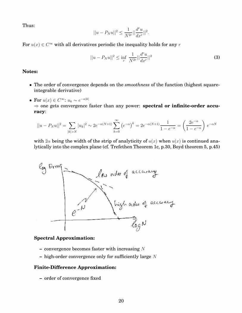
Spectral Approximation:
– convergence becomes faster with increasing N
– high-order convergence only for sufficiently large N
Finite-Difference Approximation:
– order of convergence fixed
20

• Effective exponent of convergence depends on N :
Note: in general
||dru
dxr||2 → ∞ faster than exponentially for r → ∞
– Example
||dreiqx
dxr|| = qr||eiqx||
Thus, for simple complex exponential || dr
dxr eiqx|| grows exponentially in r.
– For functions that are not given by a finite number of Fourier modes the norm
has to grow with r faster than exponentially:
show by contradiction
If ||dru
dxr||2 ∝ η2r then EN ∝
( η
N
)2r
Can then pick a fixed N > η to get
infrEN = 0
⇒ approximation is exact for finite N in contradiction to assumption..
Now consider
lnEN ≤ ln
(
infr
1
N2r||d
ru
dxr||2)
= infr
(
ln ||dru
dxr||2 − 2r lnN
)
||drudxr ||2 grows faster than exponential ⇒ ln ||dru
dxr ||2 grows faster than linearly for large r
r
small Nlarge N
⇒ can pick N sufficiently large that for small r denominator N r grows faster in r⇒ error estimate decreases with rfor larger r the exponential N r does not grow fast enough
⇒ error estimate grows with rvalue of r at the minimum gives effective exponent for decrease in error in this regime
of N .
With increasing N the minimum in the error estimate (solid circle in the figure) is
shifted to larger r⇒ effective order of accuracy increases with N :
21

Note:
Spectral approximation guaranteed to be superior to finite difference methods
only in highly accurate regime
Approximation of Derivatives
Given u(x) =∑uke
ikx the derivatives are given by
dnu
dxn=
∞∑
|k|=0
(ik)nukeikx
if the series for the derivative converges (again, convergence in the mean)
Note:
• not all square-integrable functions have square-integrable derivatives
dθ
dx= δ(x)
• if series for u(x) converges uniformly then its 1st derivative still converges (possibly
not uniformly)
• convergence for dqudxq is a power of N q slower than that for u since one can take only q
fewer derivatives of it than of u,
dqu
dxq=∑
k
(ik)quk eikx
coefficients (ik)quk decay more slowly than uk itself.
the estimate (3) gets weakened by
||dqu
dxq− PN
dqu
dxq||2 ≤ inf
r
1
N2r−2q||d
ru
dxr||2 for r > q
• Periodic boundary conditions: non-periodic derivative drudxr equivalent to discontinuous
drudxr , i.e.
dr+1udxr+1 not square-integrable
2.2 The Gibbs Phenomenon
Consider convergence in more detail for u(x) piecewise continuous
PNu(x) =
N∑
|k|=0
ukeikx =
1
2π
∫ 2π
0
N∑
|k|=0
e−ikx′+ikxu(x′) dx′
PN can be written more compact using
DN(s) ≡N∑
|k|=0
eiks =sin(N + 1
2)s
sin(12s)
.
22
This identity can be shown by multiplying by the denominator:
(
ei 12s − e−i 1
2s) [e−iNs + e−i(N−1)s + ...+ eiNs
]= ei(N+ 1
2)s − e−i(N+ 1
2)s
Insert
PNu(x) =1
2π
∫ 2π
0
sin[(N + 1
2)(x− x′)
]
sin[
12(x− x′)
] u(x′) dx′
=︸︷︷︸
use t=x−x′
1
2π
∫ x
x−2π
sin(N + 12)t
sin 12t
u(x− t) dt
Use the completeness of the Fourier modes
limN→∞
DN (s) =∞∑
|k|=0
eiks = 2π∞∑
l=−∞δ(s+ 2πl)
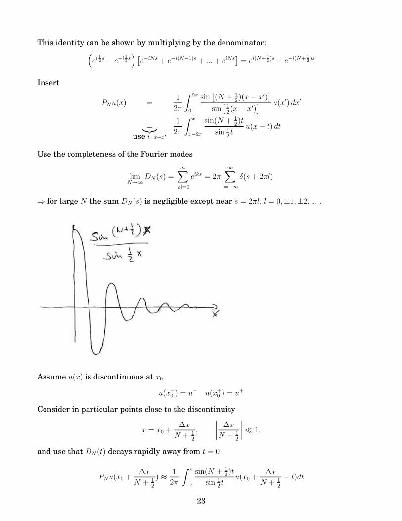
⇒ for large N the sum DN (s) is negligible except near s = 2πl, l = 0,±1,±2, ... .
Assume u(x) is discontinuous at x0
u(x−0 ) = u− u(x+0 ) = u+
Consider in particular points close to the discontinuity
x = x0 +∆x
N + 12
,
∣∣∣∣
∆x
N + 12
∣∣∣∣≪ 1,
and use that DN(t) decays rapidly away from t = 0
PNu(x0 +∆x
N + 12
) ≈ 1
2π
∫ ǫ
−ǫ
sin(N + 12)t
sin 12t
u(x0 +∆x
N + 12
− t)dt
23

Approximate u(x) in the integrand by u+ and u−, respectively,
PNu(x0 +∆x
N + 12
) ≈ 1
2πu+
∫ ∆x
N+ 12
−ǫ
sin(N + 12)t
12t
dt+1
2πu−∫ ǫ
∆x
N+ 12
sin(N + 12)t
12t
dt
Now write s = (N + 12)t and consider N → ∞ for fixed ǫ
∫ ∆x
−(N+ 12)ǫ
sin s
sds →
∫ ∆x
−∞
sin s
sds
=
∫ 0
−∞
sin s
sds+
∫ ∆x
0
sin s
sds
=π
2+ Si(∆x)
with Si(x) the sine integral and limx→∞ Si(x) = π/2.
Similarly:
∫ ǫ(N+ 12)
∆x
sin s
sds →
∫ ∞
∆x
sin s
sds
=1
2
∫ ∞
−∞
sin s
sds+
∫ 0
∆x
sin s
sds
=π
2− Si(∆x)
Thus
PNu(x0 +∆x
N + 12
) ≈ 1
2(u+ + u−) +
1
πSi(∆x)(u+ − u−)
Note:
24
• Maximal overshoot is 9% of the jump (independent of N)
PNu(x0 +π
N + 12
) − u+ = (u+ − u−)
(1
πSi(π) − 1
2
)
= (u+ − u−) 0.09
• Location of overshoot at x0 + πN+ 1
2
converges to jump position x0. Everywhere else
series converges pointwise to u(x)
• the maximal error does not decrease: convergence is not uniform in x; but convergencein the L2-norm, since area between PNu and u goes to 0.
• Smooth oscillation can indicate severe problem: unresolved discontinuity.
To capture true discontinuity finite differences may be better.
• Smooth step (e.g. tanh x/ξ):as long as step is not resolved expect behavior like for discontinuous function
slow convergence and Gibbs overshoot (⇒HW), only when enough modes are retained
to resolve the step the exponential convergence will set in.
2.3 Discrete Fourier Transformation
We had continuous Fourier transformation
u(x) =∞∑
|k|=0
eikxuk
with
uk =1
2π
∫ 2π
0
e−ikxu(x)dx
Consider evolution equation
∂u
∂t= F (u,
∂u
∂x)
Our goal was to do the time-integration completely in Fourier space since our variables are
the Fouriermodes ⇒ need Fourier components Fk
Consider linear PDE:
• F (u, ∂∂x
) = ∂2xu
∂u
∂t=∂2u
∂x2
Insert Fourier expansion and project onto φk = eikx
duk
dt= −k2uk
Consider nonlinear PDEs:
25

• Polynomial: F (u) = u3
Fk = 12π
∫
u(x)3e−ikx dx =1
2π
∫
dx e−ikx∑
k1
eik1xuk1
∑
k2
eik2xuk2
∑
k3
eik3xuk3
=∑
k1
∑
k2
uk1uk2uk−k1−k2
convolution requires N2 multiplication of three numbers, compared to a single such
multiplication
for rth−order polynomial need N r−1operations: slow!
• General nonlinearities, e.g.
coupled pendula
F (u) = sin(u) = 1 − 1
3!u3 +
1
5!u5 + ...
Arrhenius law in chemical reactions
F (u) = eu =
∞∑
l=0
1
l!ul
arbitrarily high powers of u, cannot use convolution
Evaluate nonlinearities in real space:
need to transform efficiently between real space and Fourier space
Discrete Fourier transformation:
Question: will we loose spectral accuracy with only 2N grid points in integral?
trapezoidal rule 1211111..111
2with 2N collocation points
xj =2π
2Nj, ∆x =
2π
2N, x2N = x0
uk =1
ck
1
2N
(
1
2e−ikx0u(x0) +
2N−1∑
j=1
e−ikxju(xj) +1
2e−ikx2Nu(x2N)
)
=︸︷︷︸
for periodic u(x)
1
ck
1
2N
2N−1∑
j=0
e−ikxju(xj)
High wavenumbers:
26
Calculate high wavenumber components
uN+m =1
2N
2N−1∑
j=0
e−iN 2π2N
j︸ ︷︷ ︸
e−iπj
e−imxj u(xj)
=1
2N
2N−1∑
j=0
e+iπj e−imxj u(xj)
= u−N+m
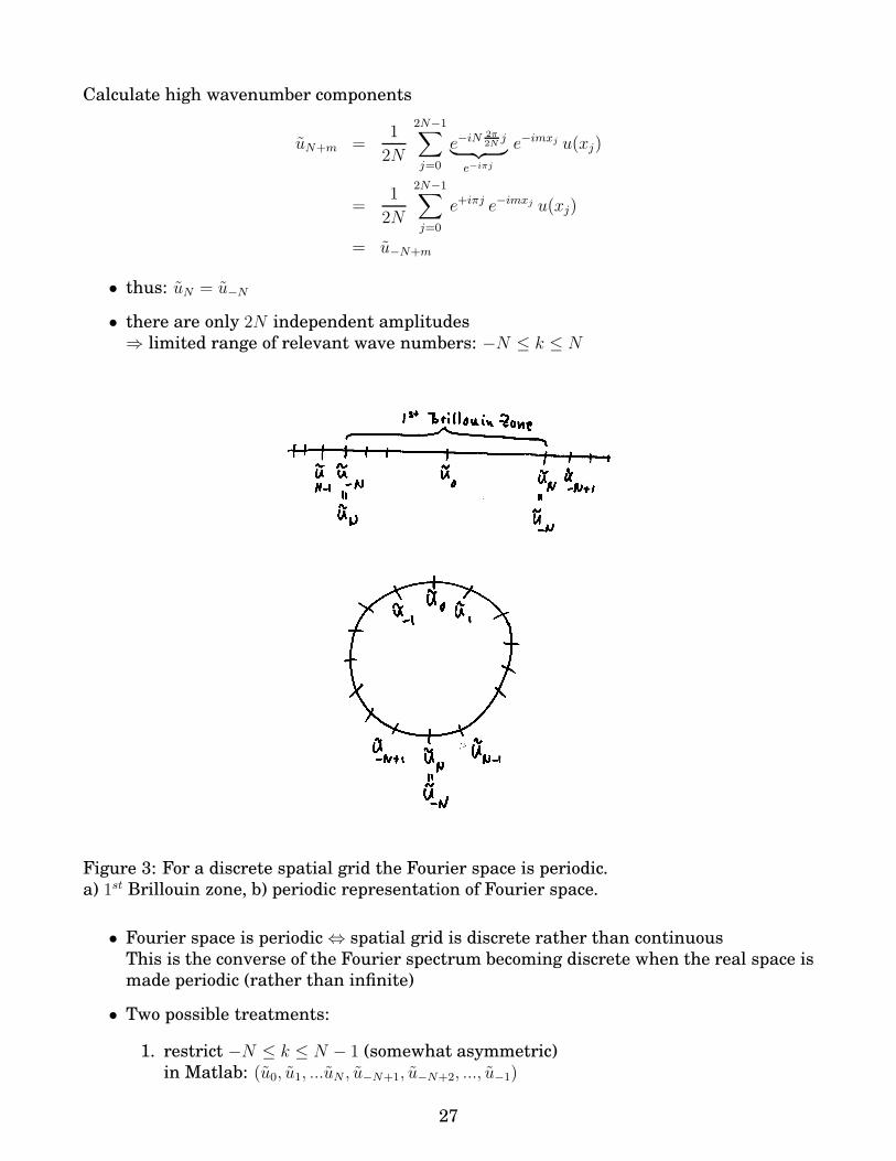
• thus: uN = u−N
• there are only 2N independent amplitudes
⇒ limited range of relevant wave numbers: −N ≤ k ≤ N
Figure 3: For a discrete spatial grid the Fourier space is periodic.
a) 1st Brillouin zone, b) periodic representation of Fourier space.
• Fourier space is periodic ⇔ spatial grid is discrete rather than continuous
This is the converse of the Fourier spectrum becoming discrete when the real space is
made periodic (rather than infinite)
• Two possible treatments:
1. restrict −N ≤ k ≤ N − 1 (somewhat asymmetric)
in Matlab: (u0, u1, ...uN , u−N+1, u−N+2, ..., u−1)
27

2. in these notes we set
uN = u−N =1
2
1
2N
2N−1∑
j=0
eiNxju(xj)
i.e.
cN = c−N = 2 and cj = 1 for j 6= ±N
Inverse Transformation
IN(u(xj)) =
N∑
k=−N
ukeikxj
Orthogonality:
< φk, φl >N=1
2N
2N−1∑
j=0
ei(l−k) 2π2N
j =
∞∑
l−k=−∞δl−k,2Nm (4)
Notation:
< ., . >N denotes the scalar product of functions defined only at N discrete points xj
Figure 4: Cancellation of the Fourier modes in the sum. Here N = 4 and l − k = 1
Note:
• < φk, φl >N 6= 0 if k − l is any multiple of 2N and not only for k = l (cf. completeness
relation (2))
high wavenumbers are not necessarily perpendicular to low wavenumbers
Interpolation property
Consider IN (u) on the grid
IN(u(xl)) =
N∑
k=−N
ukeikxl
28

=N∑
k=−N
1
2N
1
ck
2N−1∑
j=0
e−ikxju(xj)eikxl interchange sums to get δ-function
=1
2N
2N−1∑
j=0
u(xj)
2N∑
r≡k+N=0
ei(r−N) 2π2N
(l−j) 1
cr−N
in the r-sum: for r = 2N we have eiπ(l−j) 12and for r = 0 we have e−iπ(l−j) 1
2
⇒ using (4) the sum adds up to 2Nδlje−iπ(l−j) (note that |l − j| < 2N)
Thus
IN (u(xl)) =1
2N
2N−1∑
j=0
u(xj) 2Nδjl = u(xl).
Notes:
• On the grid xj the function u(x) is represented exactly by IN(u(x));no information lost on the grid
• IN (u(x)) is often called Fourier interpolant.
2.3.1 Aliasing
For the discrete Fourier transform the function is defined only on the grid:
what happens to the high wavenumbers that cannot be represented on that grid?
Consider u(x) = ei(r+2N)x with 0 < |r| < N .
Continuous Fourier transform: PNu = 0 since the wavenumber is higher than N .
Discrete Fourier transform:
u(xj) = ei(2N+r) 2π2N
j = eir 2π2N
j = eirxj
On the grid u(x) looks like eirx:
IN(u(xj)) = eirxj 6= 0
u(x) is folded back into the 1st Brillouin zone.
Notes:
• highest wavenumber that is resolvable on the grid: |k| = N
e±iN 2π2N
j = (−1)j
• in CFT unresolved modes are set to 0
• in DFT unresolved modes modify the resolved modes: Aliasing
29

Relation between CFT (uk) and DFT (uk) coefficients:
uk =1
2N
1
ck
2N−1∑
j=0
e−ikxju(xj)
=1
2N
1
ck
∞∑
l=−∞
2N−1∑
j=0
ei(l−k) 2π2N
jul
=1
ck
∞∑
l=−∞
∞∑
m=−∞δl−k,2Nmul
uk =1
ckuk +
1
ck
∞∑
|m|=1
uk+2Nm
The sum contains the aliasing terms from higher harmonics that are not represented on
the grid.
High wavenumbers look like low wavenumbers and contribute to low-k amplitudes
Error ‖u− INu‖2:
INu =
N∑
k=−N
ukeikx =
N∑
k=−N
1
ckuk +
1
ck
∞∑
|m|=1
uk+2Nm
eikx
= PNu+RNu
||u−INu||2 = || u− PNu︸ ︷︷ ︸
all modes have |k|>N
− RNu︸︷︷︸
all modes have |k|≤N
||2 =︸︷︷︸
orthogonality
||u−PNu||2+||RNu||2
Interpolation error is larger than projection error.
Decay of coefficients:
if CFT coefficients decay exponentially, uk ∼ e−α|k|, so will the DFT coefficients:
uk ∼ 1
cke−α|k|+
1
ck
∞∑
|m|=1
e−α|k+2Nm| ∼︸︷︷︸
geometric series
∼ 1
cke−α|k|+
1
ck
2e−2αN
1 − e−2αNfor k ≪ N
Thus:
The asymptotic convergence properties of the DFT are essentially the same as those of the
CFT ⇒ homework assignment
30

2.3.2 Differentiation
Main reason for spectral approach: derivatives
For CFT one has: projection and differentiation commute :
d
dx(PNu) =
N∑
k=−N
ikukeikx
PN(du
dx) =
N∑
k=−N
(du
dx)ke
ikx
=
N∑
k=−N
1
2π
∫
e−ikx′ du
dx′dx′ eikx using i.b.p. :
=N∑
k=−N
1
2πik
∫
e−ikx′
u(x′)dx′ eikx
=d
dx(PNu)
For DFT interpolation and differentiation do not commute:
d
dx(INu) 6= IN(
du
dx).
i.e. ddx
(INu) does not give the exact values of dudx
on the grid points.
INu does not agree with u between grid points ⇒ its derivative does not agree with the
derivative of u on the grid points, but IN(dudx
) does interpolate dudx.
Asymptotically, the errors of In(dudx
) and of ddxIN(u) are of the same order.
Implementation of Discrete Fourier Transformation
Steps for calculating derivatives at a given point:
i) Transform method
31

1. calculate uk from values at collocation points xj :
uk =1
2N
1
ck
2N−1∑
j=0
e−ikxju(xj)
2. for rth−derivativedru
dxr⇒ (ik)ruk
3. back-transformation at collocation points
dr
dxrIN(u(xj)) =
N∑
k=−N
(ik)rukeikxj
Notes:
• seems to require O(N2) operationscompared to O(N) operations for finite differences
• for N = 2l3m5n... DFT can be done in O(N lnN) operations using fast Fourier trans-
form1
• for u real: uk = u∗−k ⇒ need to calculate only half the uk:
special FFT that stores the real data in a complex array of half size
N independent variables: u0 and uN real, u1,...,uN−1 complex
ii) Matrix multiplication method
dr
dxr IN(u) is linear in u(xj) ⇒ can write it as matrix multiplication
dr
dxrIN(u(xj)) =
N∑
k=−N
(ik)rukeikxj interchange sums
=
2N−1∑
l=0
(N∑
k=−N
(ik)r 1
2N
1
ckeik(xj−xl)
)
u(xl)
write in terms of vectors and matrix
u(x0)...
u(x2N−1)
= udr
dxrIN(u) =
...u(r)(xj)
...
Then first derivative
u(1) = Du
1In matlab functions FFT and IFFT.
32

with
Djl =1
2N
N∑
k=−N
ik1
ckeik 2π
2N(j−l) =
12(−1)j+l cot( j−l
2Nπ) for j 6= l
0 for j = l
Higher derivatives
u(r) = Dru
Notes:
• D is 2N × 2N matrix (j, l = 0, ..., 2N − 1)
• D is anti-symmetric: Dlj = −Djl
• matrix multiplication is expensive: N2 operations
but multiplication can be vectorized, i.e. different steps of multiplication/addition are
done simultaneously for different numbers in the matrix
Eigenvalues of Pseudo-Spectral Derivative:
Fourier modes with |k| ≤ N − 1 are represented exactly
Deikx = ik eikx for |k| ≤ N − 1
⇒ plane waves eikx must be eigenvectors with eigenvalues
λk = ik = 0,±1i,±2i, ...,±(N − 1)i
D has 2N eigenvalues: one missing
trD = 0 ⇒∑
k λk = 0 ⇒ last eigenvalue λN = 0
can see that also via: eiN 2π2N
j = (−1)j = e−iN 2π2N
j ⇒ eigenvalue must be independent of the
sign of N ⇒ λN = 0
Interpretation: consider PDE
∂u
∂t=∂u
∂xwith u = eiωt+ikx
Frequency ω numerically determined by Du: ω = λk
For |k| ≤ N − 1 the solution is a traveling wave with direction of propagation given by sign
of k.
For k = ±N one has u(xj) = (−1)j : does not define a direction of propagation ⇒ ω ≡ λk = 0.
Note:
One gets a vanishing eigenvalue also using the transform method:
(−1)j = uNeiN 2π
2Nj + u−Ne
−iN 2π2N
j with uN = u−N
thusd
dxPN
((−1)j
)= iNuNe
iNxj + (−iN)u−Ne−iNxj = 0.
33

3 Fourier Methods for PDE: Continuous Time
Consider PDE∂u
∂t= S(u) ≡ F (u,
∂u
∂x,∂2u
∂x2, ...)
The operator S(u) can be nonlinear
Two methods
1. Pseudo-spectral:
u⇒ INu
Spatial derivatives in Fourier space
Nonlinearities in real space
temporal evolution performed in real space or in Fourier space:
i.e. unknowns to be updated are the u(xj) in real space or the uk in Fourier space
2. Galerkin method
u⇒ PNu
completely in Fourier space: spatial derivatives, nonlinearities and temporal updating
are all done in Fourier space
3.1 Pseudo-spectral Method
Method involves the steps
1. introduce collocation points xj and u(xj)
2. transfrom numerical solution u(xj) ⇒ uk to Fourier space
3. evaluate derivatives using uk
4. transform back into real space and evaluate nonlinearities
5. evolve in time either in real space or in Fourier space
d
dtIN(u) = S(IN(u))
Note:
IN (u) is not the spectral interpolant of the exact solution u since solving PDE induces errors:
34

1. taking the spectral interpolant of the exact solution u yields
IN
(d
dtu
)
= IN (S(u)) .
Usingd
dtIN(u) = IN
(d
dtu
)
the pseudospectral solution satisfies
IN
(d
dtu
)
= S(IN(u)) 6= IN (S(u))
since spatial derivative does not commute with IN
2. time-stepping introduces errors beyond the spectral approximation.
Examples:
1. Wave equation
∂tu = ∂xu
a) Using FFT
∂tu(xj) = ∂xIN (u(xj)) =
N∑
k=−N
ikukeikxj
Note: uk and the sum over k (=back-transformation) are evaluated via two FFTs.
b) Using multiplication with spectral differentiation matrix D,
∂tu(xj) =∑
l
Djlu(xl)
2. Variable coefficients
∂tu = c(x)∂xu
a)
∂tu(xj) = c(xj) ∂xIN(u(xj))
multiply by wave speed in real space
b)
∂tu(xj) = c(xj)∑
m
Djmu(xm).
3. Reaction-diffusion equation
∂tu = ∂2xu+ f(u)
a) using FFT
∂tu(xj) = ∂2xIN(u(xj)) + f(u(xj)) = −
N∑
k=−N
k2ukeikxj + f(u(xj))
b) matrix multiplication
∂tu(xj) =∑
m
D(2)jmu(xm) + f(u(xj)) with D
(2)jm =
∑
l
DjlDlm.
35

4. Burgers equation
∂tu = u∂xu
=1
2∂x(u
2) in conservation form
consider both types of nonlinearities2 αu∂xu+ β∂x(u2)
a)
αu(xj)∂xIN(u(xj)) = αu(xj)N∑
k=−N
ik ukeikxj
β ∂xIN(u2(xj)) = β
N∑
k=−N
ik wkeikxj
wk =1
2N
2N−1∑
j=0
e−ikxj u2(xj)
b)
∂tu(xj) = αu(x)Du+ βD
u(x0)2
...u(x2N−1)
2
Notes:
• spectral methods will lead to Gibbs oscillations near the shock
• pseudo-spectral methods: on the grid the oscillations may not be visible; may
need to plot function between grid points as well, but derivatives show oscilla-
tions
• all sums over Fourier modes k or grid points j should be done via FFT.
3.2 Galerkin Method
Equation solved completely in Fourier space
1. plug
u(x) =
N∑
k=−N
ukeikx
into ∂tu = S(u)
2. project equation onto first 2N Fourier modes (−N ≤ l ≤ N)
∂tul ≡1
2π
∫ 2π
0
e−ilx∂tu(x) dx =1
2π
∫ 2π
0
e−ilx S(u(x)) dx
2Note: For smooth functions the two formulations are equivalent.Burgers equation develops shocks at
which the solution becomes discontinuous: formulations not equivalent, need to satisfy entropy condition,
which corresponds to adding a viscous term ν∂2
xu and letting ν → 0.
36
More generally, retaining N modes from a complete set of functions {φk(x)}
u(x) =
N∑
k=1
ukφk(x)
< φl, ∂tu > = < φl, S(u) > for 1 ≤ l ≤ N
< φl, ∂tu− S(u) > = 0
Residual (=error) ∂tu− S(u) has to be orthogonal to all basis functions that were kept:
PN (∂tPNu− S(PNu)) = 0
optimal choice within the space of N modes that is used in the expansion
Note: for Galerkin the integrals are calculated exactly either analytically or numerically
with sufficient resolution (number of grid points →∞)
Examples:
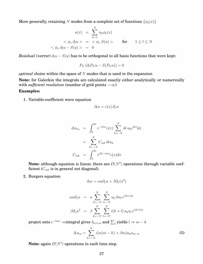
1. Variable-coefficient wave equation
∂tu = c(x) ∂xu
∂tum =
∫ 2π
0
e−imxc(x)
N∑
k=−N
ik ukeikxdx
=N∑
k=−N
Cmk ikuk
Cmk =
∫ 2π
0
ei(k−m)xc(x)dx
Note: although equation is linear, there are O(N2) operations through variable coef-
ficient (Cmk is in general not diagonal).
2. Burgers equation
∂tu = αu∂xu+ β∂x(u2)
αu∂xu = α
N∑
k=−N
N∑
l=−N
uk ilul ei(k+l)x
β∂xu2 = β
N∑
k=−N
N∑
l=−N
i(k + l) ukul ei(k+l)x
project onto e−imx ⇒integral gives δk+l,m and∑
l yields l ⇒ m− k
∂tum =N∑
k=−N
i(α(m− k) + βm)ukum−k (5)
Note: again O(N2) operations in each time step.
37

Comparison:
• Nonlinear problems:
Galerkin: effort increases with degree of nonlinearity because of convolution
pseudo-spectral: effort mostly in transformation to and from Fourier space: FFT es-
sential
• Variable coefficients:
Galerkin requires matrix multiplication, pseudospectral only scalar multiplication
• error larger in pseudo-spectral, but same scaling of error with N
• Unresolved modes:
Pseudo-spectral has aliasing errors: unresolved modes spill into equations for re-
solved modes
Nonlinearities generate high-wavenumber modes: their aliasing can be removed by
taking more grid points (32−rule) or by phase shifts
• Grid effects:
pseudo-spectral method breaks the translation symmetry, can lead to pinning of fronts
Galerkin method does not break translation symmetry.
• Newton method for unstable fixed points or implicit time stepping:
quite clear for Galerkin code: (5) is simply a set of coupled ODEs, not so obvious to im-
plement for pseudo-spectral code, since back- and forth-transformations are needed.
4 Temporal Discretization
Consider
∂tu = S(u)
Two possible goals:
1. interested in steady state: transient towards steady state not relevant
only spatial resolution relevant
2. initial-value problem: interested in complete evolution
temporal error has to be kept as small as spatial error
If transient evolution is relevant then spectral accuracy in space best exploited
if high temporal accuracy is obtained as well: seek high-order temporal schemes
38

4.1 Review of Stability
Consider ODE
∂tu = λu (6)
Definitions:
1. A scheme is stable if there are constants C, α, T , and δ such
||u(t)|| ≤ Ceαt||u(0)||for all 0 ≤ t ≤ T , 0 < ∆t < δ. The constants C and α have to be independent of ∆t.
2. A scheme is absolutely stable if
||u(t)|| <∞ for all t.
Note:
• The concept of absolute stability is only useful for differential equations for which
the exact solution is bounded for all times.
• absolute stability closely related to Neumann stability
3. The region A of absolute stability is given by the region A the complex plane defined
by
A = {λ∆t ∈ C | ||u(t)|| bounded for all t}
Notes:
• for λ ∈ R the ODE (6) corresponds to a parabolic equation like ∂tu = ∂2xu in Fourier
space
• for λ ∈ iR the ODE (6) corresponds to a hyperbolic equation like ∂tu = ∂xu in Fourier
space
For a PDE one can think in terms of a system of ODEs coupled through differentiation
matrices,
∂tu = Lu
e.g. for ∂tu = ∂xu one has L = D.
Assume L can be diagonalized
SLS−1 = Λ with Λ diagonal
Then
∂tSu = ΛSu
Thus:
Stability requires that all eigenvalues λ of L are in the region of absolute stability of the
scheme.
Note:
39

• highest Fourier eigenvalues
– for simple wave equation: λmax = ±i (N − 1)
– for diffusion equation: λmax = −N2
Side Remark: Stability condition after diagonalization in terms of Su,
||Su(t)|| < Ceαt||Su(0)||
We need
||u(t)|| < Ceαt||u(0)||If S is unitary, i.e. if S−1 = S+we have
||Su|| = ||u||
For Fourier modes spectral differentiation matrix is normal
D+D = DD+
⇒ D can be diagonalized by unitary matrix
(Not the case for Chebyshev basis functions used later)
Thus: for Fourier method it is sufficient to consider scalar equation (6).
4.2 Adams-Bashforth Methods
Based on rewriting in terms of integral equation
un+1 = un +
∫ tn+1
tn
F (t′, u(t′))dt′
Explicit method: approximate F (u) by polynomial that interpolates F (u) over last l time
steps3 and extrapolate to the interval [tn, tn+1].
Figure 5: Adams-Bashforth methods interpolate F (u) over the interval [tn−l, tn] and then
extrapolate to the interval [tn, tn+1].
3Figure has wrong label for first grid point.
40

Consider
∂tu = F (u)
AB1: un+1 = un + ∆tF (un)
AB2: un+1 = un + ∆t
(3
2F (un) − 1
2F (un−1)
)
Note:
• AB1 identical to forward Euler
Stability:
Consider F (u) = λu with λ ∈ C
AB1:
z = 1 + ∆tλ
|z|2 = (1 + λr∆t)2 + λ2
i ∆t2
Stability limit given by |z|2 = 1:
AB1=FE: (1 + λr∆t)2 + λ2
i ∆t2 = 1
To plot stability limit parametrize z = eiθ and plot λ∆t ≡ (λr(θ) + iλi(θ))∆t
AB1:
λ∆t = z − 1
AB2:
λ∆t =z − 132− 1
2z
−2.5 −2 −1.5 −1 −0.5 0 0.5−1.5
−1
−0.5
0
0.5
1
1.5Adams−Bashforth
AB1AB2AB3
41

Notes:
• AB1=FE and AB2 are not absolutely stable for purely dispersive equations λr = 0
• AB3 and AB4 are absolutely stable even for dispersive equations λr = 0
• AB1 and AB2: the stability limit is tangential to λr = 0: for λr = 0 exponential growth
rate goes to 0 for ∆t → 0 at fixed number of modes (i.e. fixed λ). For fixed tmax we can
choose ∆t small enough to limit the growth of solution.
AB1: for λr = 0 |z|2 = 1 + λ2i ∆t
2
|z| tmax∆t = (1 + λ2
i ∆t2)
12
tmax∆t ≤ e
12λ2
i ∆t2 tmax∆t need ∆t≪ O(λ−2
i )
for simple wave equation one has then
∆t≪ O(N−2)
i.e. AB1 is stable for ‘diffusive scaling’
AB2: for λr = 0 z = 1 + iλi∆t−1
2λ2
i ∆t2 +
1
4λ3
i ∆t3 − 1
8λ4
i ∆t4
|z|2 = 1 +1
2λ4
i ∆t4
|z| tmax∆t ≤ e
14λ4
i ∆t4 tmax∆t need ∆t≪ O(λ
− 43
i ) = O(N− 43 )
For simple wave equation one gets
∆t≪ O(N− 43 )
which is less stringent than AB1=FE.
The growth may be less of a problem for spectral methods since one would like to
balance the temporal error with the spatial error
∆tp ∼ e−αN
one may have to choose therefore quite small ∆t just to achieve the desired accuracy,
independent of the stability condition.
But: growth rate is largest for largest wavenumbers k: high Fourier modes tend to
‘creep in’.
• Diffusion equation: FE stability limit for λi = 0 and λr = −k2 < 0:
∆t <2
|λr|=
2
k2max
=2
N2
for central difference scheme
∆t <1
2∆x2 =
1
2
(2π
2N
)2
≈ 5
N2
The scaling of stability limit is the same, but finite-difference scheme has slightly
larger prefactor, i.e. it has a slightly larger stability range. But it needs smaller ∆xto achieve the same spatial accuracy.
42
Comment on Implementation
Consider
∂tu = ∂2xu+ f(u)
Forward Euler
un+1 = un + ∆t ∂2xu
n + ∆t f(un)
Want to evaluate derivative in Fourier space ⇒ FFT
1. If we do the temporal update in Fourier space
un+1k = un
k + ∆t(−k2)unk + ∆tFk(f(un))
where Fk(f(un)) is the kth-mode of the Fourier transform of f(un)After updating un+1
k transform back to un+1(xj) and calculate f(un+1j ) for next Euler
step.
2. If we do the temporal update in real space
First transform back into real space and do time the step there
un+1j = un
j + ∆t∂2xIN(u) + ∆t f(uj)
Note: the choice between these two types of updates is quite common, not only in
forward Euler.
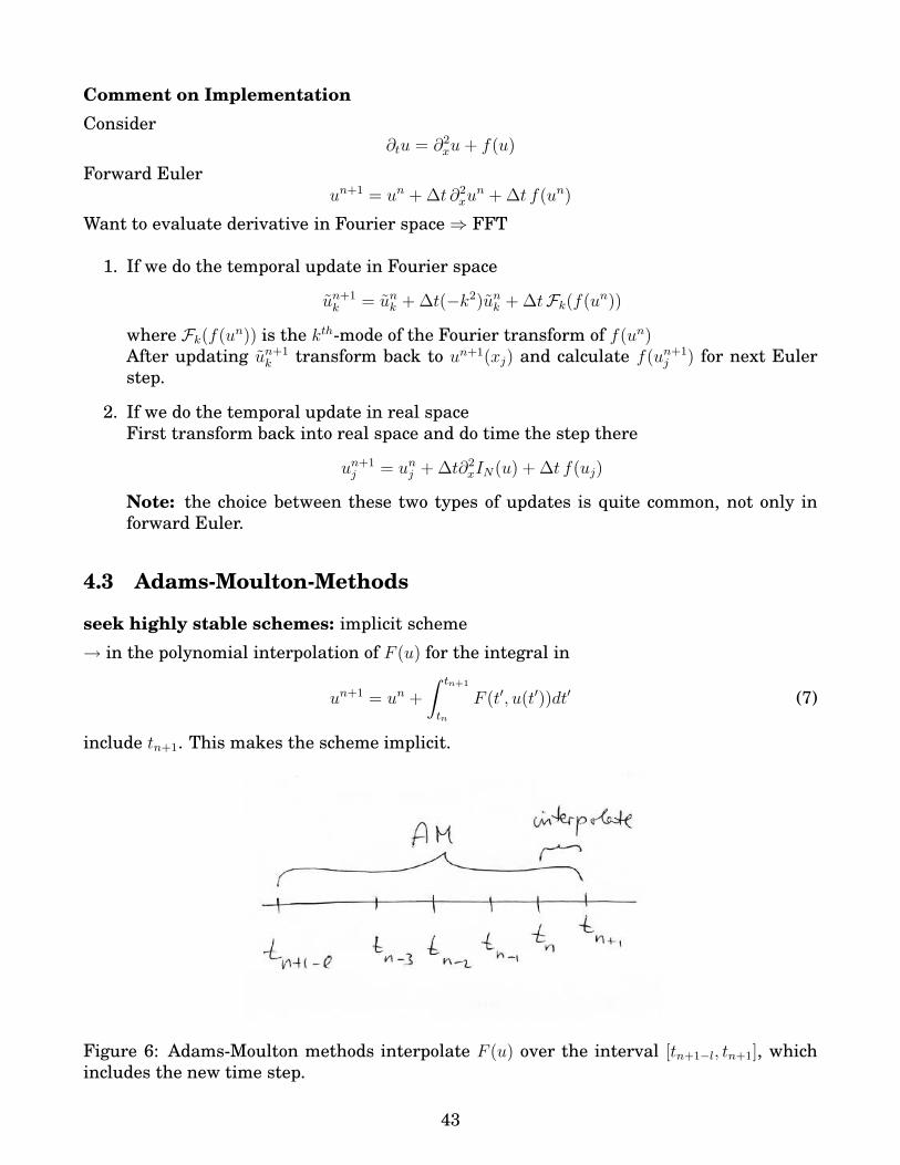
4.3 Adams-Moulton-Methods
seek highly stable schemes: implicit scheme
→ in the polynomial interpolation of F (u) for the integral in
un+1 = un +
∫ tn+1
tn
F (t′, u(t′))dt′ (7)
include tn+1. This makes the scheme implicit.
Figure 6: Adams-Moulton methods interpolate F (u) over the interval [tn+1−l, tn+1], which
includes the new time step.
43

Backwards Euler : un+1 = un + ∆tF (un+1)
Crank-Nicholson : un+1 = un +1
2∆t(F (un+1) + F (un)
)
3rd order Adams-Moulton: un+1 = un +1
12∆t(5F (un+1) + 8F (un) − F (un−1)
)
−7 −6 −5 −4 −3 −2 −1 0 1−4
−3
−2
−1
0
1
2
3
4Adams−Moulton
AM3AM4AM5AM6
Note:
• Region of stability shrinks with increasing order
• Only backward Euler and Crank-Nicholson are unconditionally stable
• AM3 and higher have finite stability limit: we do not get a high-order unconditionally
stable schem with AM.
Implementation of Crank-Nicholson
Consider the wave equation
∂tu = ∂xu(
1 − 1
2∆t ∂x
)
un+1 =
(
1 +1
2∆t ∂x
)
un
With matrix multiply method
∑
l
(
1 − 1
2∆tDjl
)
un+1(xl) =∑
l
(
1 +1
2∆tDjl
)
un(xl)
would have to invert full matrix: slow
44

With FFT or for Galerkin insert u(x) =∑
k eikxuk and project equation onto φk:
∫ 2π
0dx e−ikx...
(
1 − 1
2∆t ik
)
un+1k =
(
1 +1
2∆t ik
)
unk
un+1k =
1 + 12∆t ik
1 − 12∆t ik
unk
Note:
• Since derivative operator is diagonal in Fourier space, inversion of operator on l.h.s.
is simple:
time-stepping in Fourier space yields explicit code although implicit scheme.
This is not possible for finite differences.
• With variable wave speed one would have(
1 − 1
2∆t c(x) ∂x
)
un+1 =
(
1 +1
2∆t c(x) ∂x
)
un
⇒FFT does not lead to diagonal form: wavenumbers of u(x) and of c(x) couple⇒projection leads to convolution of c(x) and ∂xu
n+1: expensive
• The scheme does not get more involved in higher dimensions
e.g. for diffusion equation in two dimensions
∂tu = ∇2u
one gets
un+1kl =
1 − ∆t (k2 + l2)
1 + ∆t(k2 + l2)un
kl
That is to be compared with the case of finite differences where implicit schemes in
higher dimensions become much slower since the band width of the matrix becomes
large (O(N) in two dimensions, worse yet in higher dimensions).
Note:
• make scheme explicit by combining Adams-Moulton with Adams-Bashforth to predictor-
corrector
replace the unknown un+1 in the integrand of (7) of the AM-scheme by an estimate
based on AB, which can be lower order than the AM-scheme:
AB: predictor O(∆tn−1)
AM: corrector O(∆tn)
⇒ O(∆tn)
each time step requires two evaluations of r.h.s ⇒not worth if expensive
Advantage: scheme has same accuracy as AB of O(∆tn) but greater range of stability
with same storage requirements
45

4.4 Semi-Implicit Schemes
Often time step is limited by instabilities due to linear derivative terms but not due to
nonlinear terms:
Treat
• linear derivative terms implicitly
• nonlinear terms explicitly
Note: implicit treatment of nonlinear terms would require matrix inversion at each time
step
Example: Crank-Nicholson-Adams-Bashforth (CNAB)
Consider
∂tu = ∂2xu+ f(u)
un+1 − un
∆t=
1
2∂2
xun+1 +
1
2∂2
xun +
3
2f(un+1) − 1
2f(un) + O(∆t3)
(
1 − 1
2∆tD2
)
un+1 =
(
1 +1
2∆tD2
)
un + ∆t
(3
2f(un+1) − 1
2f(un)
)
3 Steps:
• FFT F of r.h.s.
• divide by (1 + 12∆tk2)
• do inverse FFT of r.h.s. ⇒un+1j
un+1j = F−1
(1
1 + 12∆tk2
{(
1 − 1
2∆t k2
)
F(uni ) + ∆tF
(3
2f(un
i ) −1
2f(un−1
i )
)})
or written as
un+1k =
1
1 + 12∆tk2
{(
1 − 1
2∆t k2
)
F(uni ) + ∆t
(3
2fk(u
ni ) −
1
2fk(u
n−1i )
)}
4.5 Runge-Kutta Methods
Runge-Kutta methods can be considered as approximations for the integral equation
un+1 = un +
∫ tn+1
tn
F (t′, u(t′))dt′
with approximation of F based purely on times t′ ∈ [tn, tn+1].
46

Runge-Kutta 2:
trapezoidal rule for integral
∫ tn+1
tn
F (t′, u(t′))dt′ =1
2∆t(F (tn, u
n) + F (tn+1, un+1)
)+ O(∆t3)
approximate un+1 with forward Euler (its error contributes to the error in the overall
scheme at O(∆t3).
Improved Euler method (Heun’s method)
k1 = F (tn, un)
k2 = F (tn + ∆t, un + ∆t k1)
un+1 = un +1
2∆t (k1 + k2) + O(∆t3)
Other version : mid-point rule ⇒ modified Euler:
un+1 = un + ∆tF
(
t+1
2∆t, un +
1
2∆tF (tn, u
n)
)
Note:
• Runge-Kutta methods of a given order are not unique (usually free parameters)
General Runge-Kutta scheme:
un+1 = un + ∆ts∑
l=0
γlFl
F0 = F (tn, un)
Fl = F (tn + αl∆t, un + ∆t
l∑
m=0
βlmFm) 1 ≤ l ≤ s
Notes:
• Scheme has s + 1 stages
• F (u) is evaluated at intermediate times tn +αl∆t and at suitably chosen intermediate
values of the function u.
• For βll 6= 0 scheme is implicit
• Coefficients αl, βlm, γl determined by requiring highest order of accuracy:
in general this does not determine the coefficients uniquely
47

Runge-Kutta 4
corresponds to Simpson’s rule (16(1 4 1))
k1 = F (tn, un)
k2 = F (tn +1
2∆t, un +
1
2∆t k1)
k3 = F (tn +1
2∆t, un +
1
2∆t k2)
k4 = F (tn + ∆t, un + ∆t k3)
un+1 = un +1
6∆t (k1 + 2k2 + 2k3 + k4) + O(∆t)5
Note:
• to push the error to O(∆t5) the middle term in Simpson’s rule has to be split up into
two different terms.
−5 −4 −3 −2 −1 0 1 2
−3
−2
−1
0
1
2
3
Runge−Kutta
RK1RK2RK3RK4
Notes:
• stability regions expand with increasing order
• RK4 covers parts of imaginary and of real axis: suited for parabolic and hyperbolic
problems
48

4.6 Operator Splitting
For linear wave equation or diffusion equation we have exact solution in Fourier space,
∂tu = ∂2xu ⇒ un
k = uk(0) e−k2tn
Can we make use of that for more general problems?
For finite differences we discussed
∂tu = (L1 + L2)u
solution approximated as
un+1 = e(L1+L2)∆tun
= eL1∆teL2∆tun + O(∆t2)
this corresponds to
∂tu = L2u and then ∂tu = L1u
alternating integration of each equation for a full time step ∆t
Apply to reaction-diffusion equation
∂tu = ∂2xu+ f(u)
L1u ∼ ∂2xu L2u ∼ f(u)
Treat L2u in real space, e.g. forward Euler
u∗(xj) = un(xj) + ∆t f(un(xj))
Treat L1u in Fourier space
un+1k = e−k2∆tu∗k exact!!
Written together:
un+1k = e−k2∆t (un
k + ∆t fk(unl ))
Notes:
• could use any other suitable time-stepping scheme for nonlinear term: higher-order
would be better
• But: operator splitting error arises.
Could improve
e(L1+L2)∆tun = e12L1∆teL2∆te
12L1∆tun + O(∆t3)
If intermediate values need not be available the 12∆t−steps can be combined:
un+2 = e12L1∆teL2∆te
12L1∆te
12L1∆teL2∆te
12L1∆tun + O(∆t3) =
= e12L1∆teL2∆teL1∆teL2∆te
12L1∆tun + O(∆t3)
approximate eL2∆t by second-order scheme (rather than forward Euler) to get over-all
error of O(∆t3).
• time-stepping is done in real space and in Fourier space
• to get higher order one would have to push the operator splitting error to higher order.
49
4.7 Exponential Time Differencing and Integrating Factor Scheme
Can we avoid the operator-splitting error altogether?
Consider again reaction-diffusion equation
∂tu = ∂2xu+ f(u)
without reaction the equation can be integrated exactly in Fourier space
un+1k = e−k2∆tun
k
Go to Fourier space (‘Galerkin style’)
∂tuk = −k2uk + fk(u) (8)
Here fk(u) is k−component of Fourier transform of nonlinear term f(u)
To assess a good approach to solve (8) it is good to consider simpler problem yet:
∂tu = λu+ F (t) (9)
where u is the Fourier mode in question and F plays the role of the coupling to the other
Fourier modes.
We are in particular interested in efficient ways to deal with the fast modes with large,
positive λ because they set the stability limit:
1. If the overall solution evolves on the fast time scale set by λ, accuracy requires a time
step with |λ∆t| ≪ 1 and an explicit scheme should be adequate.
2. If the overall solution evolves on a slower time scale τ ≫ 1/|λ|, which is set by Fourier
modes with smaller wavenumber (i.e. F (t)evolves slowly in time) then one would like
to take time steps with |λ|∆t = O(1) or even larger without sacrificing accuracy, i.e.
one would like to be limited only by the condition ∆t≪ τ .In particular, for F = const. one would like to obtain the exact solution u∞exact = −F/λwith large time steps.
Use integrating factor to rewrite (9) as
∂t
(ue−λt
)= e−λtF (t)
which is equivalent to
un+1 = eλ∆tun + eλ∆t
∫ ∆t
0
e−λt′F (t+ t′)dt′.
Need to approximate integral. To leading order it is tempting to write
un+1 = eλ∆tun + eλ∆t∆t F (t).
This yields the forward Euler implementation of the integrating-factor scheme.
For F = const. this yields the fixed point
u∞IF
(1 − eλ∆t
)= ∆t eλ∆t F.
But:
50
• for −λ∆t ≫ 1 one has u∞IF → 0 independent of F and definitely not u∞IF → u∞exact ≡−F/λ. To get a good approximation of the correct fixed point u∞exact one therefore still
needs |λ|∆t≪ 1!
Note:
• even for simple forward Euler fixed point (un+1 = un) would be obtained exactly for
large ∆t (disregarding stability)
un+1 = un + ∆t (λun + F )
Problem: Even if F evolves slowly, for large λ the integrand still evolves quickly over the
integration interval: to assume the integrand is constant is a poor approximation.
Instead: assume only F is evolving slowly and integrate the exponential explicitly
un+1 = eλ∆tun + eλ∆tF (tn)1
λ
(1 − e−λ∆t
)
This yields the forward Euler implementation of the exponential time differencing scheme,
un+1 = eλ∆tun + ∆t F (tn)
(eλ∆t − 1
λ∆t
)
Notes:
• now, for F = const and −λ∆t → ∞ one gets the exact solution u∞ETD → −F/λ.
• for |λ|∆t≪ 1 one gets back the usual forward Euler scheme (eλ∆t − 1)/λ∆ → 1.
For the nonlinear diffusion equation one gets for ETDFE
un+1k = e−k2∆tun
k + ∆t Fk(ul(t))
(
1 − e−k2∆t
k2∆t
)
where in general Fk(ul(t)) depends on all Fourier modes uk.
For higher-order accuracy in time use better approximations for the integral (see Cox &
Matthews, J. Comp. Physics 176 (2002) 430, and Kassam & Trefethen, SIAM J. Sci. Com-
put. 26 (2005) 1214, for a detailed discussion of various schemes and quantitative compar-
isons for ODEs and PDEs. The latter paper includes two matlab programs for Fourier and
Chebyshev spectral implementations).
The 4th-order Runge-Kutta version reads (using c ≡ λ∆t)
u1k = unk E1 + ∆t Fk(u
n, tn)E2
u2k = unk E1 + ∆t Fk(u1, tn +
1
2∆t)E2
u3k = u1k E1 + ∆t
(
2Fk
(
u2, tn +1
2∆t
)
− Fk (un, tn)
)
E2
un+1k = un
kE21 + ∆t ·G
G = Fk (un, tn) E3 + 2
(
Fk
(
u1, tn +1
2∆t
)
+ Fk
(
u2, tn +1
2∆t
))
E4 + (10)
+Fk (u3, tn + ∆t) E5
51

with
E1(c) = ec/2 E2(c) =ec/2 − 1
c
E3(c) =−4 − c+ ec (4 − 3c+ c2)
c3
E4(c) =2 + c+ ec (−2 + c)
c3
E5(c) =−4 − 3c− c2 + ec (4 − c)
c3
For |c| < 0.2 the factors E3,4,5(c) can become quite inaccurate due to cancellations:
E5(c) =1
c3
(
−4 − 3c− c2 +
(
1 + c+1
2c2 +
1
6c3 + . . .
)
(4 − c)
)
=1
6+ O(c)
For small values of c it is therefore better to replace E3,4,5 by their Taylor expansions
E2(c) =1
2+
1
8c+
1
48c2 +
1
384c3 +
1
3840c4 +
1
46080c5 +
1
645120c6 +
1
10321920c7
E3(c) =1
6+
1
6c+
3
40c2 +
1
45c3 +
5
1008c4 +
1
1120c5 +
7
51840c6 +
1
56700c7
E4(c) =1
6+
1
12c+
1
40c2 +
1
180c3 +
1
1008c4 +
1
6720c5 +
1
51840c6 +
1
453600c7
E5(c) =1
6+ 0 c− 1
120c2 − 1
360c3 − 1
1680c4 − 1
10080c5 − 1
72576c6 − 1
604800c7
Alternatively, one can evaluate the coefficients via complex integration using the Cauchy
integral formula [7]
f(z) =1
2πi
∮
C
f(t)
t− zdt (11)
if f(z) is analytic inside C which encloses z. Since the singularities of Ei(c) at c = 0 are
removable and since C can be chosen to remain a finite distance away from c = 0 the
Cauchy integral formula (11) can be used to evaluate Ei(c) even in the vicinity of c = 0.
Note:
• diffusion and any other linear terms retained in the eigenvalue λ of the linear operator
are treated exactly
• no instability arises from the linear terms for any ∆t : unconditionally stable
• to evaluate Fk(u1, tn + 12∆t):
u1k
inverse FFT︷︸︸︷→ u1(xj)
insert into F︷︸︸︷→ F (u1, tn +
1
2∆t)
FFT︷︸︸︷→ Fk(u1, tn +
1
2∆t)
• if the PDE involves multiple components (e.g. u and v in a two-component reaction-
diffusion system) at each stage of the RK4-scheme one needs to determine the analo-
gous quantities uik and vik with i = 1, 2, 3 in parallel, i.e. one needs to determine both
u1k and v1k before one can proceed to u2k and v2k etc.
52

• large wave numbers are strongly damped, as they should be (this is also true for
operator splitting)
compare with Crank-Nicholson (in CNAB, say)
un+1k =
1 − 12∆t k2
1 + 12∆t k2
unk
for large k∆t
un+1k = −(1 − 4
∆t k2+ ...)un
k
which exhibits oscillatory behavior and slow decay.
Note that backward Euler also damps high-wavenumber oscillations, but it is only
first order
un+1k =
1
1 + ∆tk2un
k → 1
∆tk2un
k for |k| → ∞.
Note:
• some comments on the 4th-order integrating factor scheme are in Appendix B.
4.8 Filtering
In some problems it is not (yet) possible to resolve all scales
• shock formation (cf. Burgers equation last quarter)
• fluid flow at high Reynolds numbers (turbulence): energy is pumped in at low wavenum-
bers (e.g. by motion of the large-scale walls), but only very high wavenumbers experi-
ence significant damping, since for low viscosity high shear is needed to have signifi-
cant damping.
In these cases aliasing and Gibbs oscillations can lead to problems.
Aliasing and Nonlinearities
Nonlinearities generate high wavenumbers
u(x)2 =N∑
l=−N
N∑
k=−N
ulukei(k+l)x
p-th order polynomial generates wavenumbers up to ±pN . On the grid of 2N points not all
wavenumbers can be represented ⇒ Fourier interpolant IN(u(x)) keeps only ±N : higher
wavenumber aliased into that range.
Example:
53
on grid xj = 2π2Nj with only 2 grid points per wavelength 2π
qwith q = N
u(xj) = cos qxj = cosN2π
2Nj = cos(πj) = (−1)j
u(xj)2 = cos2 qxj = (+1)j = 1 cos2 qxj is aliased to a constant on that grid
Note: in a linear equation no aliasing arises during the simulation since no high wavenum-
bers are generated (aliasing only initially when initial condition is reduced to the discrete
spatial grid)
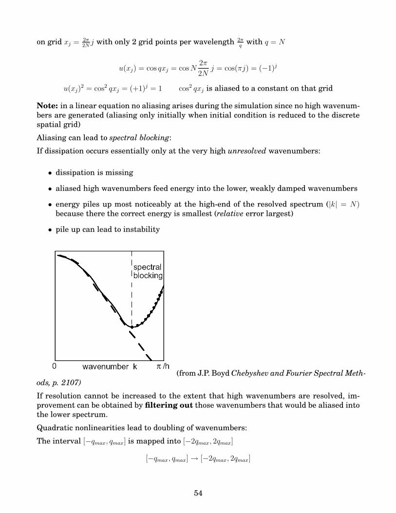
Aliasing can lead to spectral blocking:
If dissipation occurs essentially only at the very high unresolved wavenumbers:
• dissipation is missing
• aliased high wavenumbers feed energy into the lower, weakly damped wavenumbers
• energy piles up most noticeably at the high-end of the resolved spectrum (|k| = N)because there the correct energy is smallest (relative error largest)
• pile up can lead to instability
(from J.P. Boyd Chebyshev and Fourier Spectral Meth-
ods, p. 2107)
If resolution cannot be increased to the extent that high wavenumbers are resolved, im-
provement can be obtained by filtering out those wavenumbers that would be aliased into
the lower spectrum.
Quadratic nonlinearities lead to doubling of wavenumbers:
The interval [−qmax, qmax] is mapped into [−2qmax, 2qmax]
[−qmax, qmax] → [−2qmax, 2qmax]
54

-N N
q 2q2q-2N
Require that the mapped wavenumber interval does not alias into the original wavenumber
interval
2qmax − 2N ≤ −qmax
i.e. require
qmax ≤ 2
3N
More generally: for pth-order nonlinearity choose
qmax =p+ 1
2N
Algorithm:
1. FFT: ui → uk
2. take derivatives
3. filter out high wavenumbers: uk = 0 for |k| > p+12N
4. inverse FFT: uk → ui; this function does not contain any ‘dangerous’ high wavenum-
bers any more
5. evaluate nonlinearities ui → upi
6. back to 1.
(from J.P. Boyd Chebyshev
and Fourier Spectral Methods, p. 212)
55

Orszag’s 2/3-rule:
For quadratic nonlinearity set the highest N/3 Fourier-modes to 0 in each time step just
before the back-transformation to the spatial grid:
• evaluating the quadratic nonlinearity (which is done in real space):
– the ‘good’ wavenumbers [0, 23N ] contained in u(x) generate the wavenumbers [0, 4
3N ]
of which the interval [N, 43N ] will be aliased into [−N,−2
3N ] and therefore will
contaminate the highest N/3 modes (analogously for [0,−23N ]).
– the ‘bad’, highest N/3 modes [23N,N ] generate wavenumbers [4
3N, 2N ] which are
aliased into [−23N, 0] and would contaminate the ‘good’ wavenumbers.
• setting the highest N/3 modes to 0 avoids contamination of good wavenumbers; no
need to worry about contaminating the high wavenumbers that later are set to 0
anyway.
Alternative view:
For a quadratic nonlinearity, to represent the wavenumbers [−N,N ] without aliasing need32· 2N grid points:
want 3N grid points for integrals ⇒ before transforming the Fourier modes [−N,N ] back to
real space need to pad them with zeroes to the range [−32N, 3
2N ].
Thus: To avoid aliasing for quadratic nonlinearity need 3 grid points per wavelength
cos qxj = cos(N2π
3Nj) = cos(2π
j
3)
Notes:
• for higher nonlinearities larger portions of the spectrum have to be set to 0.
• instead of step-function filter can use smooth filter, e.g.
F (k) =
1 |k| ≤ k0 (= 23N)
e−(|k|n−|k0|n) |k| > k0
(12)
with n = 2, 4.
• 23−rule (and the smooth version) makes the pseudo-spectral method more similar to
the projection of the Galerkin approach
• does not remedy the missing damping of high wavenumbers, but reduces the (incor-
rect) energy pumped into the weakly damped wave numbers.
56

Gibbs Oscillations
Oscillations due to insufficient resolution can contaminate solution even away from the
sharp step/discontinuity: can be improved by smoothing
Approximate derivatives, since they are more sensitive to oscillations (function itself does
not show any oscillations on the grid)
∂xu⇒N∑
k=−N
ik ukeikx filter to
N∑
k=−N
ik F (k) ukeikx
with F (k) as in (12).
Note:
• result is different than simply reducing number of modes since the number of grid
points for the transformation is still high
• filter could also smooth away relevant oscillations ⇒ loose important features of solu-
tion
e.g. interaction of localized wave pulses: oscillatory tails of the pulses determine the
interaction between the pulses, smoothing would kill interaction
Notes:
• It is always better to resolve the solution
• Filtering and smoothing make no distinction between numerical artifacts and physi-
cal features
• Shocks would better be treated with adaptive grid
57

5 Chebyshev Polynomials
Goal: approximate functions that are not periodic
5.1 Cosine Series and Chebyshev Expansion
Consider h(θ) on 0 ≤ θ ≤ π
extend to [0, 2π] to generate periodic function by reflection about θ = π
g(θ) =
h(θ) 0 ≤ θ ≤ π
h(2π − θ) π ≤ θ ≤ 2π
Then
g(θ) =
∞∑
k=−∞gke
ikθ =
∞∑
k=−∞gk(cos kθ + i sin kθ)
Reflection symmetry: sin θ drops out
g(θ) =∞∑
k=−∞gk cos kθ =
∞∑
k=0
gk cos kθ
with
gk = gk for k = 0 gk = 2gk for k > 0
gk =1
2π
∫ 2π
0
e−ikθg(θ)dθ =1
π
∫ π
0
cos kθg(θ)dθ reflection symmetry
Write as
gk =1
π
2
ck
∫ π
0
cos kθ g(θ)dθ with ck =
2 for k = 0
1 for k > 0
58

This is the cosine transform.
Notes:
• Convergence of the cosine series depends on the odd derivatives at θ = 0 and θ = π
• If dgdθ
6= 0 at θ = 0 or θ = π then gk = O(k−2) even if function is perfectly smooth in
(0, π):
gk =2
πck
∫ π
0
cos kθ g(θ)dθ i.b.p
=2
πck
1
ksin kθ g(θ)
∣∣∣∣
π
0
− 2
πck
1
k
∫ π
0
sin kθd
dθg(θ)dθ i.b.p
=2
πck
1
k2cos kθ
d
dθg(θ)
∣∣∣∣
π
0
− 2
πck
1
k2
∫ π
0
cos kθd2
dθ2g(θ)dθ
boundary terms vanish for all k only if
g′(0) = 0 = g′(π)
Since cos kπ = (−1)k non-zero slopes at the endpoints cannot cancel for all k.
• in general, only odd derivatives of g(θ) contribute to boundary terms:
1
kl+1cos kθ
dl
dθlg(θ)
∣∣∣∣
π
0
for l odd
Thus:
• for general boundary conditions Fourier (=cosine) series converges badly: Gibbs phe-
nomenon
59

5.2 Chebyshev Expansion
To get the derivative of the function effectively to vanish at the boundaries stretch the
coordinates at the boundaries infinitely strongly. This can be achieved by parametrizing xusing the angle θ on a circle:
Consider f(x) on −1 ≤ x ≤ 1
Transform to 0 ≤ θ ≤ π using x = cos θ, g(θ) = f(cos(θ))
Function is now parametrized by θ instead of x
Consider Fourier series for g(θ)
g′(θ) = −f ′(cos θ) sin θ ⇒ dg
dθ= 0 at θ = 0, π
Generally: all odd derivatives of g(θ) vanish at θ = 0 and θ = π.
Proof: cos θ is even about θ = 0 and about θ = π ⇒ f(cos θ) is also even about those points
⇒ all odd derivatives vanish at θ = 0, π.
Thus: the convergence of the approximation to g(θ) by a cosine-series does not depend on
the boundary conditions on f(x)
f(x) = g(θ) =
∞∑
k=0
gk cos kθ extension of g to 2π is even
60
=
∞∑
k=0
gk cos(k arccosx)
Introduce Chebyshev polynomials
Tk(x) = cos(k arccosx) = cos kθ
f(x) =∞∑
k=0
fk Tk(x)
Properties of Chebyshev Polynomials
• Tk(x) is a kth−order polynomial
show recursively:
T0(x) = 1 T1(x) = x
Tn+1(x) = cos ((n + 1) arccosx) = cos ((n+ 1)θ)
Trig identities:
cos ((n+ 1)θ) = cosnθ cos θ − sinnθ sin θ
cos ((n− 1)θ) = cosnθ cos θ + sinnθ sin θ
cancel sinnθ sin θ by adding and use cos(θ) = T1(x) = x,
Tn+1(x) = 2xTn(x) − Tn−1(x)
Note: recursion relation useful for computation of Tn(x)
• Tn(x) even for n even, odd otherwise
• Tn(x) =∑
j ajxj ⇒ aj have alternating signs
• the expansion coefficients are given by
fk = gk =1
π
2
ck
∫ π
0
g(θ) cos kθ dθ
rewrite in terms of x:
θ = arccosx dθ =1√
1 − x2dx
fk =2
πck
∫ 1
−1
f(x)Tk(x)1√
1 − x2dx
ck =
{2 k = 01 k > 0
• The convergence of f(x) in terms of Tk(x) is the same as that of g(θ) in terms of the
cosine-series. In particular, boundary values are irrelevant (replace x by cos θ in f(x))
61
• The Chebyshev polynomials are orthogonal in the weighted scalar product
< Tk, Tl >≡∫ 1
−1
Tk(x)Tl(x)1√
1 − x2dx = ck
π
2δkl
• The weight√
1 − x2−1
is singular but
∫ 1
−1
1√1 − x2
dx
is finite.
• Derivatives of Tk(x) :
d
dxis not diagonal for basis of Tk(x)
d
dxTk(x) 6= λTk(x)
in particular: the order of the polynomial changes upon differentiation.
Considering ddθ
cos(n± 1)θ one gets
d
dxTk±1 =
d
dθcos(k ± 1)θ
dθ
dx
= −(k ± 1)1dxdθ
(sin kθ cos θ ± cos kθ sin θ)
1
k + 1
d
dxTk+1(x) −
1
k − 1
d
dxTk−1(x) =
1
sin θ(sin kθ cos θ + cos kθ sin θ − sin kθ cos θ + cos kθ sin θ)
thus
2Tk(x) =1
k + 1
d
dxTk+1(x) −
1
k − 1
d
dxTk−1(x)
Thus: differentiation more difficult than for Fourier modes.
• Zeroes of Tk(x)
Tk(x) = cos (k arccosx) = cos kθ
⇒ Tk(x) has k zeroes in [−1, 1]
kθl = (2l − 1)π
2l = 1, ..., k
xl = cos2l − 1
2kπ
The zeroes cluster near the boundaries.
62

• Extrema of Tk(x) (Chebyshev points)
kθl = lπ xl = cosl
kπ l = 1, ..., k
Tk(xl) = (−1)l
Extrema are also clustered at boundary
Chebyshev polynomial look like a cosine-wave wrapped around a cylinder and viewed
from the side
• Transformation to θ = arccos x places more points close to boundary: small neighbor-
hood dx is blown up in dθ
x = cos θ dθ = − 1
sin θdx
⇒ dθ → ∞ for θ → 0, πdf
dθ→ 0
all derivatives vanish at boundary: no Gibbs phenomenon for non-periodic functions
• understanding of properties of functions often aided by knowing what eigenvalue
problem they solve: what is the eigenvalue problem that has the Tk(x) as solutions?
Tk(x) = cos kθd2
dθ2cos kθ = −k2 cos kθ
rewrite in terms of x = cos θ
d
dθ= − sin θ
d
dx= −
√1 − x2
d
dx
thus Tk(x) satisfies the Sturm-Liouville problem
√1 − x2
d
dx
(√1 − x2
d
dxTk(x)
)
+ k2Tk(x) = 0
63
with boundary conditions: Tk(x) bounded at x = ±1Note: Sturm-Liouville problem is singular: coefficient of highest derivative vanishes
at boundary ⇒ no boundary values specified but only boundedness
The singularity is the origin of hte good boundary resolution (no Gibbs). Fourier series
is solution of regular Sturm-Liouville problem
6 Chebyshev Approximation
Approximate f(x) on a ≤ x ≤ b using Chebyshev polynomials
Again depending on the evaluation of the integrals
• Galerkin expansion
• Pseudospectral expansion
6.1 Galerkin Approximation
PNu(x) =N∑
k=0
ukTk(x)
with
uk =2
π
1
ck
∫ +1
−1
1√1 − x2
u(x)Tk(x)dx
Note:
• need to transform first from interval a ≤ t ≤ b to −1 ≤ x ≤ +1 using
x =2t− (a+ b)
b− a
Transformation to θ = arccosx showed
uk = O(k−r) if u ∈ Cr−1 (∂rxu ∈ L1)
i.e. if rth derivative is still integrable (may be a δ−function)
Show this directly in x:πck2uk =
∫1√
1 − x2u(x)Tk(x)dx
using k2Tk(x) = −√
1 − x2 ddx
(√
1 − x2 ddxTk)
πck2uk = − 1
k2
∫1√
1 − x2u(x)
√1 − x2
d
dx
(√1 − x2
d
dxTk(x)
)
dx =
= − 1
k2u(x)
√1 − x2
d
dxTk
∣∣∣∣
+1
−1
+1
k2
∫ +1
−1
du
dx
√1 − x2
d
dxTk(x)dx = since u(x) bounded
=1
k2
{
du
dx
√1 − x2Tk(x)
∣∣∣∣
+1
−1
−∫ +1
−1
d
dx
(du
dx
√1 − x2
)
Tk(x)dx
}
64
Note:
even without the 2nd integration by parts it seems that uk = O(k−2)⇒ it seems that even for d2u
dx2 /∈ L1 one gets uk = O(k−2)
But:d
dxTk(x) =
d
dxcos(k arccosx) = O(k)
⇒ for dudx
∈ L1 andd2udx2 /∈ L1:
uk = O(1
k2
d
dxTk(x)) = O(
1
k)
Again, convergence of Chebyshev approximation can be shown to be
||PNu(x) − u(x)|| ≤ C
N q||u||q
with ||u|| being the usual L2−norm (with weight√
1 − x2−1
and ||u||q being the qth Sobolev
norm
||u||2q = ||u||2 + ||dudx
||2 + ...+ ||dqu
duq||2
For derivatives one gets
||dru
dxr− dr
dxrPNu|| ∼ ||u− PNu||r ≤
C
N12+q−2r
||u||q
Note:
• for each derivative the convergence decreases by two powers of N ; in Fourier expan-
sion each derivative lowered the convergence only by a single power in N .
• for C∞−functions one still has spectral accuracy, i.e. exponential convergence
• the estimate for the rth derivative is not precisely for the derivative but for the r−Sobolev
norm (cf. [1] for details)
• rule of thumb: for each wavelength of a periodic function one needs at least 3 Cheby-
shev polynomials to get reasonable approximation.
6.2 Pseudo-Spectral Approximation
For Galerkin approximation the projection integral
uk =2
πck
∫ π
0
u(cos θ) cos kθdθ
has to be calculated exactly (e.g. analytically)
For pseudospectral approximation calculate integral based on a finite number of collocation
points.
Strategy: find most accurate integration formula for the functions in question
65

Here: u(cos θ) is even in θ ⇒ u(cos θ) cos kθ has expansion in cosnθ
⇒ need to consider only cosnθ when discussing integration method
Analytically we have ∫ π
0
cosnθ dθ = π δn0
Similar to Fourier case: use trapezoidal rule
∫ π
0
g(θ) dθ ⇒N∑
j=0
g(πj
N)π
Ncjwith cj =
2 j = 0, N
1 otherwise
Show: Trapezoidal rule is exact for cos lθ, l = 0, ..., 2N − 1
1. l = 0∫
dθ ⇒N∑
j=0
g(πj
N)π
Ncj=
π
2N+ (N − 1)
π
N+
π
2N
2. l even
cos lθj =1
2(eilθj + e−ilθj ) with θj =
π
Nj
⇒N∑
j=0
1
cjeil π
Nj =
︸︷︷︸
eilπ=e0 for l even
N∑
j=1
(eil π
N
)j
= eil πN
1 − eilπ
1 − eil πN
= 0 using
N∑
j=1
qj = q1 − qN
1 − q
Note: for l = 2N the denominator vanishes:
cos 2Nπ
Nj = 1 ⇒
∑
6= 0 trapezoidal rule not correct
3. l odd:cos lθ odd about θ = π
2
cos lθj = − cos lθN−j
cos lθj = cos lπ
Nj
cos lθN−j = cos(
lπ
NN − l
π
Nj)
= − cos(
−l πNj)
⇒N∑
j=0
cos lθj = 0
66
Transform in x−coordinates
∫ 1
−1
p(x)√1 − x2
dx =
∫ π
0
p(cos θ)dθ =N∑
j=0
p(cosπ
Nj)
π
Ncj
Note:
This can also be viewed as a Gauss-Lobatto integration
∫ 1
−1
p(x)w(x)dx =
N∑
j=0
p(xj)wj
with points xj = cos πNj and weights wj = π
Ncj
Gauss-Lobatto integration is exact for polynomials up to degree 2N − 1:
• degree 2N − 1 polynomials have 2N coefficients
• 2N parameters to choose:
wj for j = 0, ..., N and xj for j = 1, ..., N − 1 since x0 = −1 and xN = +1
The xj are roots of a certain polynomial q(x) = pN+1(x) + apN(x) + bpN−1(x) with a and bchosen such that q(±1) = 0
Note: for the scalar product one needs the integral to be exact up to order 2N since each
factor can be a N th-order polynomial ⇒ see (13) below
Summarizing:
pseudo-spectral coefficients given by
uk =2
Nck
N∑
j=0
u(xj)Tk(xj)1
cj
with
ci =
2 i = 0, N
1 1 ≤ i ≤ N − 1
again highest mode resolvable on the grid given by
TN(xj) = cos(
N arccos(
cosπ
Nj))
= cosπj = (−1)j
Remember origin of ck
cN = 2 as in Fourier expansion in θ
c0 = 2 since only for k 6= 0 two exponentials e±ikx contribute to cos kx
Note:
• need not distinguish between ck and cj : from now on cj = cj
67
Notes:
• transformation can be written as matrix multiplication
uk =
N∑
j=0
Ckju(xj)
with
Ckj =2
NckcjTk(xj) =
2
Nckcjcos(
k arccos(cosπ
Nj))
=2
Nckcjcos(
kjπ
N)
• the inverse transformation is
u(xj) =
N∑
k=0
Tk(xj) uk =
N∑
k=0
(C−1
)
jkuk
with(C−1
)
jk= Tk(xj) = cos
πjk
N
• transformation seemingly O(N2): but there are again fast transforms (see later).
• discrete orthogonalityN∑
j=0
Tl(xj)Tk(xj)1
cj=N
2clδlk
since for l + k ≤ 2N − 1 the integration is exact
N∑
j=0
Tl(xj)Tk(xj)wj =
∫
Tl(x)Tk(x)1√
1 − x2dx = ck
π
2δlk note: wj =
π
cjN
for l + k = 2N : since l, k ≤ N one has l = N = k: TN(xj) = (−1)j
⇒N∑
j=0
TN (xj)TN (xj)1
cj= N (13)
although T 2N is not a constant (only on the grid).
The pseudospectral approximant interpolates the function on the grid
INu(xl) =
N∑
k=0
ukTk(xl) =
N∑
k=0
N∑
j=0
2
Nckcju(xj)Tk(xj)Tk(xl)
68
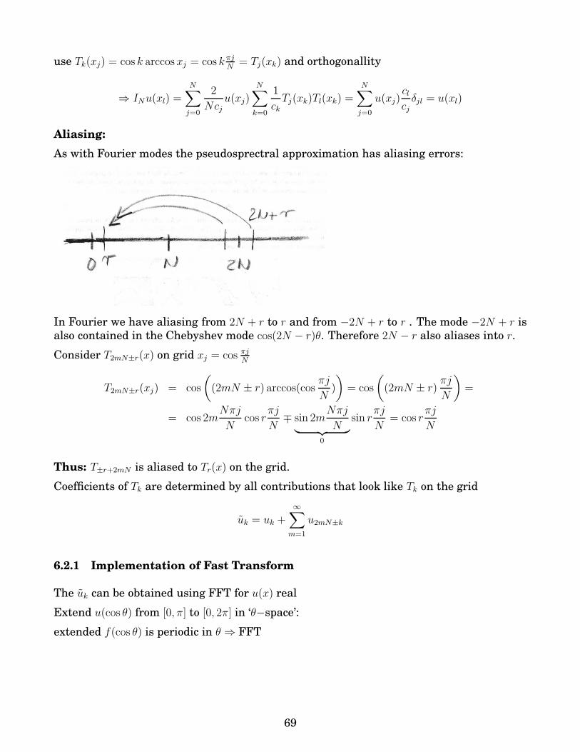
use Tk(xj) = cos k arccosxj = cos k πjN
= Tj(xk) and orthogonallity
⇒ INu(xl) =N∑
j=0
2
Ncju(xj)
N∑
k=0
1
ckTj(xk)Tl(xk) =
N∑
j=0
u(xj)clcjδjl = u(xl)
Aliasing:
As with Fourier modes the pseudosprectral approximation has aliasing errors:
In Fourier we have aliasing from 2N + r to r and from −2N + r to r . The mode −2N + r isalso contained in the Chebyshev mode cos(2N − r)θ. Therefore 2N − r also aliases into r.
Consider T2mN±r(x) on grid xj = cos πjN
T2mN±r(xj) = cos
(
(2mN ± r) arccos(cosπj
N)
)
= cos
(
(2mN ± r)πj
N
)
=
= cos 2mNπj
Ncos r
πj
N∓ sin 2m
Nπj
N︸ ︷︷ ︸
0
sin rπj
N= cos r
πj
N
Thus: T±r+2mN is aliased to Tr(x) on the grid.
Coefficients of Tk are determined by all contributions that look like Tk on the grid
uk = uk +∞∑
m=1
u2mN±k
6.2.1 Implementation of Fast Transform
The uk can be obtained using FFT for u(x) real
Extend u(cos θ) from [0, π] to [0, 2π] in ‘θ−space’:
extended f(cos θ) is periodic in θ ⇒ FFT
69

extension
uj =
{u(xj) 0 ≤ j ≤ N
u(x2N−j) N + 1 ≤ j ≤ 2N
Note:
• in Matlab the extension can be done easily using the command FLIPDIM
Coefficients are given by
uk =2
Nck
N∑
j=0
u(xj)Tk(xj)1
cj=
2
Nck
N∑
j=0
u(xj) cos(kπj
N)1
cj(14)
Rewrite the sum in terms of the extension (using that cos and u are even with respect to
θ = 0, π
N−1∑
j=1
uj cosπjk
N=︸︷︷︸
j=2N−r r=2N−j
2N−1∑
r=N+1
u2N−r︸ ︷︷ ︸
ur
cos
(πk
N(2N − r)
)
=
2N−1∑
r=N+1
ur cosπkr
N
thus considering factor 1/cj in (14)
uk =2
Nck
1
2
{
u0 cos 0 + uN cos πk + 2N−1∑
j=1
uj cosπjk
N
}
=
=2
Nck
1
2
{
u0 cos 0 + uN cos πk +
N−1∑
j=1
uj cosπjk
N+
2N−1∑
j=N+1
uj cosπjk
N
}
=1
Nck
2N−1∑
j=0
uj cosπjk
N=
1
NckRe
{2N−1∑
j=0
ujei jπk
N
}
︸ ︷︷ ︸
FFT
Notes:
• here the ordering of grid points is x = cos θtherefore u0 = u(+1) and uN = u(−1)
70
Reorder:
zj = cos θN−j then z0 = −1 zN = +1
Tk(zj) = cos (k arccos cos θN−j) = cos(
k(N − j)π
N
)
= cos kπ coskjπ
N+ sin kπ sin
kjπ
N= (−1)k cos
kjπ
N
Thus:
Tk(zj) = (−1)kTk(xj)
expressing the fact that reflecting about the y-axis (x → −x) amounts to switching sign of
the odd Chebyshev polynomials but leaving the even Tk unchanged.
Relation to FFT is changed
uk =2
Nck
N∑
j=0
u(xj)Tk(xj)1
cj=︸︷︷︸
relabeling
2
Nck
N∑
j=0
u(zj)Tk(zj)1
cj
= (−1)k 2
Nck
N∑
j=0
u(zj) coskjπ
N
1
cj= (−1)k 1
NckRe
{2N−1∑
j=0
uj ei jπk
k
}
︸ ︷︷ ︸
FFT
where
u0 = u(−1) uN = u(+1) u2N = u(−1)
⇒ with natural ordering FFT yields (−1)kuk.
6.3 Derivatives
Goal: approximate derivative of u(x) by derivative of interpolant INu(x)
Need ddxTk(x) in terms of Tk(x). We had
Recursion Relation
d
dxTm+1(x) = (m+ 1)
{
2Tm(x) +1
m− 1
d
dxTm−1(x)
}
m ≥ 2
withd
dxT0(x) = 0
d
dxT1(x) = T0
Note:
• ddxTm−1 contains even lower Tl etc.:
ddxTm contains contributions from many Tk
71
First Derivative
Expand the derivative of the interpolant in Tk(x)
d
dx(INu(x)) =
N∑
k=0
ukd
dxTk(x) =
N∑
k=0
bkTk(x)
To determine bl project derivative onto Tl(x)
N∑
k=0
uk
∫ +1
−1
Tl(x)d
dxTk(x)
1√1 − x2
dx =
N∑
k=0
bk
∫ 1
−1
Tl(x)Tk(x)1√
1 − x2dx
︸ ︷︷ ︸
δlkπ2ck
=π
2cl bl
Note:
• here c0 = 2 and cN = 1 since full projection, integrand evaluated not only at discrete
grid points (we get an analytic result for the bk )
Use∫ 1
−1
Tl(x)d
dx(Tk(x))
1√1 − x2
dx =
0 l ≥ k0 k > l k + l evenkπ k > l k + l odd
Proof:
1. l ≥ kdegree of d
dxTkis k − 1 ⇒ can be expressed by sum of Tj with j < l; scalar product
vanishes since Tk ⊥ Tj for j 6= k
2. k + l even ⇒ l and k both even or both odd ⇒ TlddxTk odd ⇒ integral vanishes
3. k + l odd, k > l: prove by induction
write k = l + 2r − 1, r = 1, 2, 3, ...
(a) r = 1, k = l + 1first l 6= 0
< Tld
dxTl+1 > =
︸︷︷︸
recursion for ddx
Tl+1
(l+1)
2 < TlTl > +1
l − 1< Tl
d
dxTl−1 >
︸ ︷︷ ︸
=0 since l−1<l
= 2(l+1)π
2
now l = 0
< T0d
dxT1 >=< T0T0 >= π
72
(b) induction step: assume
< Tld
dxTl+2r−1 >= (l + 2r − 1)
︸ ︷︷ ︸
k
π, r ≥ 1
〈Tld
dxTl+2(r+1)−1〉 = 〈Tl(l + 2r + 1)
(
2Tl+2r +1
l + 2r − 1
d
dxTl+2r−1
)
〉
=l + 2r + 1
l + 2r − 1〈Tl
d
dxTl+2r−1〉 =
l + 2r + 1
l + 2r − 1(l + 2r − 1)π = (l + 2r + 1)π
= (l + 2(r + 1) − 1)π
Thus:
bl =2
cl
N∑
k=l+1 ; k+l odd
kuk
Notes:
• calculation of single coefficient bl is O(N) operations instead of O(1) for Fourier⇒ calculation of complete derivative seems to require O(N2) operation
• bl depends only on uk with k > l: only polynomials with higher degree contribute to a
given power of x of the derivative
Determine bl recursively:
cl2bl = (l + 1)ul+1 +
N∑
k=l+3 ; k+l odd
kuk = (l + 1)ul+1 +cl+2
2bl+2
Thus
bN = 0
bN−1 = 2NuN
clbl = 2(l + 1)ul+1 + bl+2 0 ≤ l ≤ N − 2
Note:
• here cN = 1 since full integral ⇒ no factor cl+2 for l ≤ N − 2
• recursion relation requires only O(N) operations for all N coefficients
• recursion relation cannot be parallelized or vectorized:
evaluation of bl requires knowledge of bk with k > l:
– cannot evaluate all coefficients bl simultaneously on parallel computers
– cannot start evaluating product involving bl without finishing first calculation for
bk with k > l
73

Higher Derivatives
calculate higher derivatives recursively
dn
dxnu(x) =
d
dx
(dn−1
dxn−1u(x)
)
i.e. given
dn−1
dxn−1IN(u(x)) =
N∑
k=0
b(n−1)k Tk(x)
one gets
dn
dxnIN(u(x)) =
N∑
k=0
b(n−1)k
d
dxTk(x) =
N∑
k=0
b(n)k Tk(x)
with
b(n)N = 0
b(n)N−1 = 2Nb
(n−1)N
clb(n)l = 2(l + 1)b
(n−1)l+1 + b
(n)l+2
Note:
• to get nth derivative effectively have to calculate all derivatives up to n
6.3.1 Implementation of Pseudospectral Algorithm for Derivatives
Combine the steps: given u(x) at the collocation points xj calculate ∂nxu at xj
I. Transform Method
1. Transform to Chebyshev amplitudes
uk =2
Nck
N∑
j=0
u(xj) cosjkπ
N
1
cj
2. Calculate derivatives recursively
b(n)N = 0
b(n)N−1 = 2Nb
(n−1)N
clb(n)l = 2(l + 1)b
(n−1)l+1 + b
(n)l+2
3. Transform back to real space at xj
∂nx IN (u(xj)) =
N∑
k=0
b(n)k cos
jkπ
N
74

Note:
• steps 1. and 3. can be performed using FFT
FFT for back transformation
forward transformation was
uk =2
Nck
N∑
j=0
u(xj) cosjkπ
N
1
cj=
1
NckRe
{2N−1∑
j=0
ujei πjk
N
}
(15)
the last sum can be done as forward FFT
For first derivative at xj we needN∑
k=0
bk cosjkπ
N
1. extend bjbr = b2N−r for r = N + 1, ..., 2N − 1
2. need factors cj (cf. (15)): redefine bj
b0 = 2b0 bN = 2bN bj = bj for j 6= 0, N
N∑
k=0
bk cosjkπ
N=
N∑
k=0
bk cosjkπ
N
1
ck=
1
2Re
{2N−1∑
k=0
bkei jkπ
N
}
︸ ︷︷ ︸
FFT
Last sum can again be done as forward FFT.
Notes:
• backward transformation uses the same FFT as the forward transformation.
more precisely, because only real part is taken the sign of i does not matter
• again for natural ordering want derivative at zj = cos πN
(N − j):need
bk cos
(kπ
N(N − j)
)
= (−1)kbk coskjπ
N
⇒ replace
bk → (−1)k bk
II. Matrix Multiply Approach
As in Fourier case derivative is linear in u(xj) ⇒ can be written as matrix multiplication
∂xIN(u(xj)) =
N∑
k=0
Djku(xk)
75

Djk gives contribution of u(xk) to derivative at xj
The polynomial IN(u(x)) interpolates u on the grid xj . Since the order of IN is equal to the
number of grid points, this polynomial is unique. Therefore start by seeking the polynomial
that interpolates u(xj) and then take its derivative.
Construct interpolating polynomial from polynomials gk(x) satisfying
gk(xj) = δjk
u(xj) =
N∑
k=0
gk(xj)u(xk)
∂xu(x)|xj=
N∑
k=0
∂xgk(x)
∣∣∣∣∣xj
u(xk) ≡N∑
k=1
Djku(xk)
Construct the polynomial noting that Chebyshev polynomial TN (x) has extrema at all xj
for 1 ≤ j ≤ N − 1d
dxTN(xj) = 0 for j = 1, ...N − 1
Note: ddxTN has N − 1 zeroes since it has order N − 1
gk(x) =(−1)k+1
N2ck︸ ︷︷ ︸
normalization
vanishes at x0,N
︷ ︸︸ ︷
(1 − x2)
vanishes at xj
︷ ︸︸ ︷
d
dxTN(x)
1
x− xk︸ ︷︷ ︸
cancels (x−xk) in numerator
Notes:
•∑u(xk)gk(x) interpolates u on the grid
• gk(x) is indeed a polynomial since denominator is cancelled by ddxTN , which vanishes
at the xk
• gk(x) is a Lagrange polynomial
L(N)k (x) =
N∏
k 6=m=0
x− xm
xk − xm=
x− x0
xk − x0. . .
x− xk−1
xk − xk−1
x− xk+1
xk − xk+1. . .
x− xN−1
xk − xN−1
x− xN
xk − xN0 ≤ k ≤ N
Take derivative of gk(x)
d
dxINu(xj) =
N∑
k=0
u(xk)g′k(xj) =
N∑
k=0
Djku(xk)
For natural ordering z = cos θN−j = cos N−jNπ, i.e. z0 = −1 and zN = 1, one gets
76

Djk =cjck
(−1)j+k 1
xj − xkfor j 6= k
Djj = − xj
2 (1 − x2j )
for j 6= 0, N (16)
D00 = −2N2 + 1
6DNN = +
2N2 + 1
6
Notes:
• differentiation matrix is not skew-symmetric
Djk 6= Dkj since Djj 6= 0 andcjck
• ||D|| = O(N2) because of clustering of points at the boundary
clear for D00 and DNN .
smallest grid distance is O(N−2), e.g., for |j −N | ≪ N
1 − zj = 1 − cos (θN−j) = 1 − (1 − (N − j)2
N2π2 + ...) = O(N−2)
⇒ stability condition will involve N−2 instead of N−1
⇒ more restrictive than Fourier modes
• higher derivatives obtained via Dn
Note:
• it turns out that the numerical accuracy of the matrix-multiply approach using D as
formulated in (16) is quite prone to numerical round-off errors. D has to satisfy
N∑
j=0
Dij = 0 ∀j
reflecting that the derivative of a constant vanishes.
A better implementation is
Djk =cjck
(−1)j+k 1
xj − xkfor j 6= k
Djj = −N∑
j 6=k=0
Djk (17)
(18)
7 Initial-Boundary-Value Problems: Pseudo-spectralMethod
We introduced Chebyshev polynomials to deal with general boundary conditions. Imple-
ment them now
77
7.1 Brief Review of Boundary-Value Problems
Depending on character of equation we need to pose/may pose different number of boundary
conditions at different locations.
7.1.1 Hyperbolic Problems
characterized by traveling waves: boundary conditions depend on characteristics:
Boundary condition to be posed on incoming characteristic variable but not on outgoing
characteristic variable. Solution blows up if boundary condition is posed on wrong variable.
1. Scalar wave equation
∂tu = ∂xu u(x, 0) = u0(x) − 1 ≤ x ≤ +1
wave travels to the left
u(x, t) = u(x+ vt)
distinguish boundaries;
(a) x = −1: outflow boundary ⇒ u is outgoing variable
requires and allows no boundary condition
(b) x = +1 : inflow boundary ⇒ u is incoming variable
needs and allows single boundary condition
2. System of wave equations
∂tu = A∂xu
diagonalize A to determine characteristic variables
Example:
∂tu = ∂xv
∂tv = ∂xu
Taking sum and difference
Ul = u+ v Ur = u− v
∂tUl,r = ±∂xUl,r
(a) x = −1: only Ur is incoming, only Ur accepts boundary condition
(b) x = +1: only Ul is incoming, only Ul accepts boundary condition
Physical boundary conditions often not in terms of characteristic variables
Example:
u = u± at x = ±1 v unspecified
at x = −1:
Ur(−1) = u− − v(−1) = u− − 1
2(Ul(−1) − Ur(−1))
Ur(−1) = 2u− − Ul(−1)
78
7.1.2 Parabolic Equations
No characteristics, boundary conditions at each boundary
Example:
∂tu = ∇ · j = ∇ · ∇u = ∆u
Typical boundary conditions:
1. Dirichlet
u = 0
2. Neumann (no flux boundary condition)
∂xu = 0
3. Robin boundary conditions
αu+ β∂xu = g(t)
7.2 Pseudospectral Implementation
Pseudospectral: we have grid points ⇒ boundary values available
discuss using matrix-multiply approach
Explore: simple wave equation
∂tu = ∂xu u(x = 1, t) = g(t)
discretize
∂tui =
N∑
j=0
Dijuj with uj = u(xj)
Notes:
• spatial derivative calculated using all points
⇒ derivatives available at boundaries without introducing the virtual points that ap-
peared when using finite differences
∂xu0 =1
2∆x(u1 − u−1)
• boundary condition seems not necessary: it looks as if uN could be updated without
making use of g(t).But: PDE would be ill-posed without boundary conditions
⇒ scheme should blow up! (see later)
79
Correct implementation
∂tui =N∑
j=0
Dijuj i = 0, ..., N − 1
uN = g(t)
Note:
• although uN is not updated using the PDE, it can still be used to calculate the deriva-
tive at the other points.
Express scheme in terms of unknown variables only: u0, u1, ...uN−1
Define reduced n× n−differentiation matrix
D(N)ij = Dij i, j = 0, ..., N − 1
i.e. N th row and column of Dij are omitted.
∂tui =N−1∑
j=0
D(N)ij uj +DiNuN i = 0, ..., N − 1
uN = g(t)
Notes:
• boundary conditions modify differentiation matrix
• in general equation becomes inhomogeneous
7.3 Spectra of Modified Differentiation Matrices
With u = (u0, ..., uN−1) PDE becomes inhomogeneous system of ODEs
∂tu = D(N)u + d with di = DiNg(t)
For simplicity assume vanishing boundary values: d = 0
Stability properties determined by eigenvalues λj of modified differentiation matrix D(N)
∂tuj = λjuj
Reminder:
• region of absolute stability of scheme for eigenvalue λj
{λj ∆t ∈ C|uj bounded for all t}
• scheme is asymptotically stable if it is absolutely stable for all eigenvalues of D(N)
80

7.3.1 Wave Equation: First Derivative
What are the properties of D(N)?
Review of Fourier Case
• eigenvalues of DF are ik, |k| = 0, 1, ...N − 1. All eigenvalues are purely imaginary and
the eigenvalue 0 is double.
• DF is normal ⇒ can be diagonalized by unitary matrix U
U−1DU =
λ1
λ2
...λN
≡ D
with ||D|| = ||D|| and ||U−1u|| = ||u||⇒ ||u|| is bounded by the same constant as ||U−1u||, independent of N⇒ sufficient to look at scalar equation.
Properties of D(N) for Chebyshev
• eigenvalues of D(N) are not known analytically
• eigenvalues of D(N) have negative real part
∂tu = D(N)u well-posed
∂tu = −D(N)u ill-posed
in ill-posed case boundary condition should be at x = −1 but it is posed at x = +1Example: N = 1
D(N) = D00 = −2 + 1
6= −1
2
∂tu0 = −1
2u0 bounded; boundary condition on u1
For boundary condition at x = −1 introduce D(0)
D(0)ij = Dij i, j = 1, ..., N
Thus for
∂tu = −∂xu
∂tui = −N∑
j=1
D(0)ij uj +Di0g(t) for i = 1, ..., N
Eigenvalues of D(0) have positive real part
Example: N = 1
D(0) = DNN = +1
2
Note:
81

– in Fourier real part vanishes: ⇒ no blow-up
periodic boundary conditions are well-posed for both directions of propagation
• D(N) is not normal (D+D 6= DD+) ⇒ similarity transformation S to diagonal form not
unitary
||u|| 6= ||Su||For any fixed N ||u|| is bounded if ||Su|| is boundedBut constant relating ||u|| and ||Su|| could diverge for N → ∞⇒ stability is not guaranteed for N → ∞ if scalar equation is stable.
• eigenvalues of D(N) and D(0) are O(N2)⇒ stability limits for wave equation will involve
∆t ≤ O(N−2)
larger eigenvalues reflect the close grid spacing near the boundary, ∆x = O(N−2)
7.3.2 Diffusion Equation: Second Derivative
Consider
∂tu = ∂2xu α0,N u+ β0,N ∂xu = γ0,N at x = ±1
a) Fixed Boundary Values α = 1, β = 0unknowns
u1, u2, ..., uN−1
known
u0 = γ0 uN = γN
Reduced (n− 1) × (n− 1) differentiation matrix for second derivative
D(0,N)2,ij = (D2)ij i, j = 1, ..., N − 1
then
∂tui =N−1∑
j=1
D(0,N)2,ij uj + (D2)i0γ0 + (D2)iNγN for i = 1, ..., N − 1
82

Note:
• again the 2nd derivative is calculated by using all values of u, including the fixed
prescribed boundary values
• for transformation to uk via FFT use all grid points
information for ∂2xu is, however, discarded at the boundaries
Eigenvalues
exact eigenvalues of ∂2xu with u(±1) = 0:
• sin qx is eigenfunction of ∂2x for q = π
Ln = π
2n. ⇒ eigenvalues λn = −π2
4n2
• all functions that vanish at x = ±1 can be expanded in terms of sin qxwith q = πLn = π
2n
⇒ sin qx form a complete set ⇒ no other eigenfunctions
eigenvalues of D(0,N)2 :
• all eigenvalues are real and negative
• eigenvalues are O(N4) reflecting the small grid spacing near the boundaries.
b) Fixed Flux: α = 0, β = 1Need other modification of D2:
• u0 and uN now unknown ⇒ (n + 1) × (n+ 1) matrix
• ∂xu0 and ∂xuN are known
⇒ ∂xui is calculated with D only for i = 1, ..., N − 1
D(0,N)ij =
{Dij 1 ≤ i ≤ N − 10 i = 0 or i = N
∂xui =
N∑
j=0
D(0,N)ij uj + δi,0γ0 + δi,NγN i = 0, ..., N
• 2nd derivative
∂2xui =
N∑
j=0
Dij∂xuj =
N∑
j,k=0
DijD(0,N)jk uk +Dijδj,0γ0 +Dijδj,NγN
• Diffusion equation
∂tui =
N∑
j,k=0
DijD(0,N)jk uk
︸ ︷︷ ︸
apply e.g. Crank-Nicholson
+ Di0γ0 +DiNγN︸ ︷︷ ︸
inhomogeneous terms
1
∆t
(un+1 − un
)= θDD(0,N)un+1 + (1 − θ)DD(0,N)un +Di0γ0 +DiNγN
Note:
83

– derivative at boundary is calculated also with spectral accuracy; in finite differ-
ence schemes they are one-sided: reduced accuracy
– Crank-Nicholson for fixed boundary values similar.
7.4 Discussion of Time-Stepping Methods for Chebyshev
Based on analysis ofdu
dt= λu
which scheme has range of ∆t in which it is absolutely for given λ ∈ C
Main aspect: not only D(0,N)2 but also D(N) has negative real part
7.4.1 Adams-Bashforth
AB1= forward Euler
AB2
un+1 = un + ∆t
(3
2fn − 1
2fn−1
)
AB3
un+1 = un + ∆t
(23
12fn − 16
12fn−1 +
5
12fn−2
)
−2.5 −2 −1.5 −1 −0.5 0 0.5−1.5
−1
−0.5
0
0.5
1
1.5Adams−Bashforth
AB1AB2AB3
Since the eigenvalues of the odd Chebyshev derivatives have non-zero (negative) real part
all three schemes have stable regions not only for diffusion but also for wave equation.
84
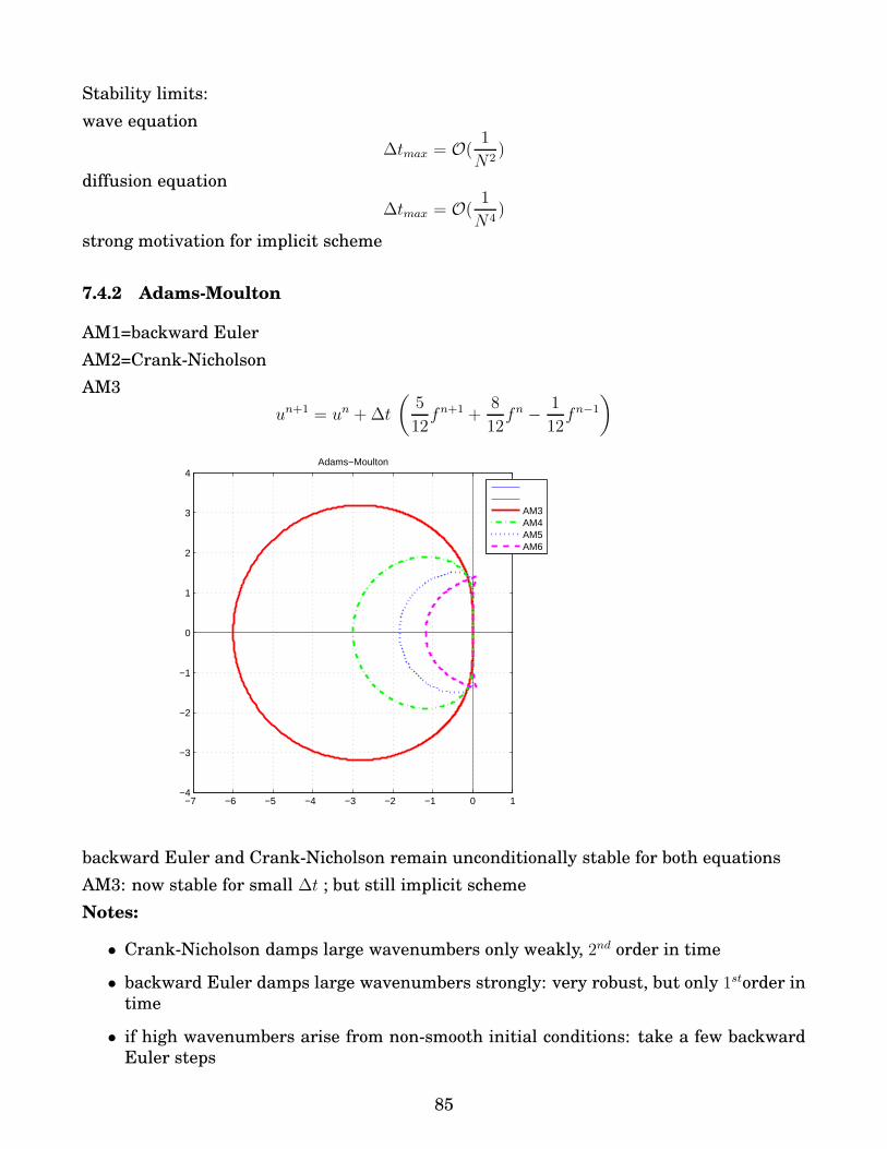
Stability limits:
wave equation
∆tmax = O(1
N2)
diffusion equation
∆tmax = O(1
N4)
strong motivation for implicit scheme
7.4.2 Adams-Moulton
AM1=backward Euler
AM2=Crank-Nicholson
AM3
un+1 = un + ∆t
(5
12fn+1 +
8
12fn − 1
12fn−1
)
−7 −6 −5 −4 −3 −2 −1 0 1−4
−3
−2
−1
0
1
2
3
4Adams−Moulton
AM3AM4AM5AM6
backward Euler and Crank-Nicholson remain unconditionally stable for both equations
AM3: now stable for small ∆t ; but still implicit scheme
Notes:
• Crank-Nicholson damps large wavenumbers only weakly, 2nd order in time
• backward Euler damps large wavenumbers strongly: very robust, but only 1storder in
time
• if high wavenumbers arise from non-smooth initial conditions: take a few backward
Euler steps
85

7.4.3 Backward-Difference Schemes
this class of schemes is obtained by obtaining interpolant for u(t) and taking its derivative
as the left-hand-side of differential equation
pm(t) =
m−1∑
k=0
u(tn+1−k)L(m)k (t)
with Lagrange polynomials
L(m)k (t) =
m−1∏
k 6=l=0
t− tn+1−l
tn+1−k − tn+1−l
to get derivativedu
dt
∣∣∣∣tn+1
=d
dtpm(t)
∣∣∣∣tn+1
1. m = 2
p2(t) =un+1 − un
tn+1 − tn(t− tn) + un
d
dtp2(t)
∣∣∣∣tn+1
=un+1 − un
tn+1 − tn= f(un+1)
thus: BD1=backward Euler
2. m = 3 yields BD23
2un+1 − 2un +
1
2un−1 = ∆t fn+1
−15 −10 −5 0 5 10 15 20 25 30 35−25
−20
−15
−10
−5
0
5
10
15
20
25backward differentiation
BD1BD2BD3BD4BD5BD6
−1 −0.5 0 0.5
−2
−1.5
−1
−0.5
0
0.5
1
1.5
2
2.5
3
backward differentiation
BD1BD2BD3BD4BD5BD6
Neumann Analysis for BD2:3
2z − 2 +
1
2z− ∆tλz = 0
86
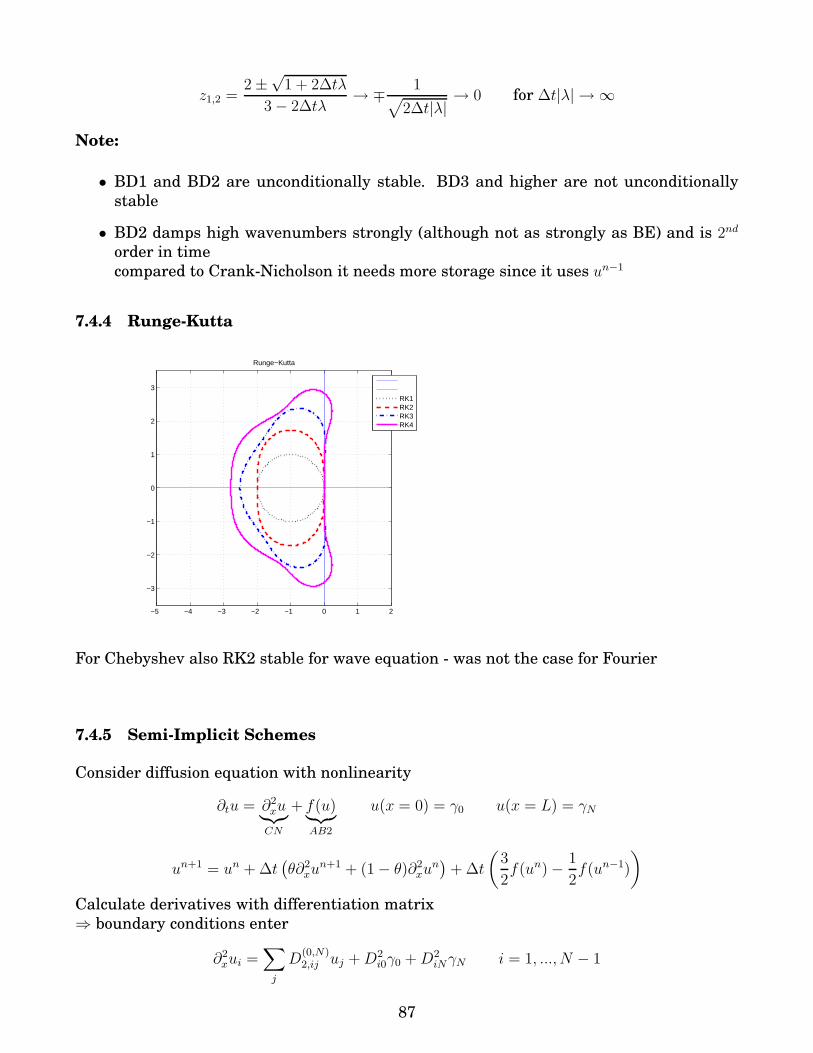
z1,2 =2 ±
√1 + 2∆tλ
3 − 2∆tλ→ ∓ 1
√
2∆t|λ|→ 0 for ∆t|λ| → ∞
Note:
• BD1 and BD2 are unconditionally stable. BD3 and higher are not unconditionally
stable
• BD2 damps high wavenumbers strongly (although not as strongly as BE) and is 2nd
order in time
compared to Crank-Nicholson it needs more storage since it uses un−1
7.4.4 Runge-Kutta
−5 −4 −3 −2 −1 0 1 2
−3
−2
−1
0
1
2
3
Runge−Kutta
RK1RK2RK3RK4
For Chebyshev also RK2 stable for wave equation - was not the case for Fourier
7.4.5 Semi-Implicit Schemes
Consider diffusion equation with nonlinearity
∂tu = ∂2xu︸︷︷︸
CN
+ f(u)︸︷︷︸
AB2
u(x = 0) = γ0 u(x = L) = γN
un+1 = un + ∆t(θ∂2
xun+1 + (1 − θ)∂2
xun)
+ ∆t
(3
2f(un) − 1
2f(un−1)
)
Calculate derivatives with differentiation matrix
⇒ boundary conditions enter
∂2xui =
∑
j
D(0,N)2,ij uj +D2
i0γ0 +D2iNγN i = 1, ..., N − 1
87

remember
D(0,N)2,ij = (D2)ij i, j = 1, ..., N − 1
insert in scheme
∑
j
(δij − ∆tθD(0,N)2,ij )un+1
j =∑
j
(δij + ∆t(1 − θ)D(0,N)2,ij )un
j + ∆t(D2
i0γ0 +D2iNγN
)+
∆t
(3
2fi(u
n) − 1
2fi(u
n−1)
)
i = 1, ..., N − 1
Notes:
• Need to invert δij − ∆tθD(0,N)2,ij : constant matrix ⇒ only one matrix inversion
• in the algorithm D(0,N)2,ij is effectively a N − 2 × N − 2 matrix; but it is not the same
matrix as D2 for N − 2 nodes!
• if boundary condition depends on time
either CN
∆t(θD2
i0γ0(tn+1) + (1 − θ)D2i0γ0(tn+1)
)
or AB2
∆t
(3
2D2
i0γ0(tn) − 1
2D2
i0γ0(tn−1)
)
4
7.4.6 Exponential Time-Differencing
Consider again
∂tu = ∂2xu+ f(u) 0 < x < L b.c. at x = 0, L
Using the Chebyshev differentiation matrix D2 this can be integrated formally
un+1 = eD2∆tun + eD
2∆t
∫ ∆t
0
e−D2t′f(t+ t′)dt′
where f denotes the vector (f1, . . . , fN).
For a EDTFE we approximate this as
un+1 = e∆tD2
un + ∆tE0(∆tD2) f(tn) (19)
4Include CNAB for Chebyshev with FFT:
(I + ∆tD)−1 = (FF−1 + ∆tF
−1DF )−1 = (F−1(I + ∆tD)F )−1 = F
−1(I + ∆tD)−1F
88

with
E0(∆tD2) = (∆tD)−2
(
I − e−D2∆t)
As in the Fourier case the evaluation of E0 suffers from round-off through cancellations.
Even worse cancellations for Ei in EDTRK4 (cf. (10)). Using Taylor’s formula is not
straightforward. Use Cauchy integral formula for matrices A [6, 7].
Consider
Φ(A) =1
2πi
∮
Cf(t) (tI −A)−1 dt
Assume A can be diagonalized
A = SΛS−1
with Λ = diag(λ1, λ2, . . . , λn)
(tI − A)−1 =(tSIS−1 − SΛS−1
)−1={S (tI −Λ)S−1
}−1
= S (tI −Λ)−1S−1 = S diag
(1
t− λ1, . . . ,
1
t− λn
)
S−1
Since S does not depend on t ∈ C
Φ(A) = S1
2πi
∮
Cf(t)diag
(1
t− λ1, . . . ,
1
t− λn
)
dtS−1
= S diag
(1
2πi
∮
Cf(t)
1
t− λ1dt, . . . ,
1
2πi
∮
Cf(t)
1
t− λndt
)
S−1
If C encloses λi1
2πi
∮
Cf(t)
1
t− λidt = f(λi)
If C encloses all eigenvalues of A one gets
Φ(A) = S diag (f(λ1), . . . , f(λn))S−1 = f(A)
and
f(A) =1
2πi
∮
Cf(t) (tI −A)−1 dt (20)
Notes:
• sample code for the Allen-Cahn equation, f(u) = u− u3, is in the appendix of [7]
• the contour integral can be evaluated using the trapezoidal rule
• simplest contour is a circle with radius R centered at t = 0
• eigenvalues of D2 grow like N4 ⇒ R has to be chosen large enough
– et grows and oscillates rapidly for ranges of large complex t (cf. (10))
89

– more integration points are needed for the integral
– possibly other contour shapes preferrable (e.g. elliptic close to real axis or parabolic)
Boundary conditions:
1. Fixed boundary values:
u0 = γ0 uN = γN
using the modified differentiation matrix D(0,N)2 we have N −1 unknowns u1, . . . , uN−1,
∂tui =N−1∑
j=1
D(0,N)2,ij uj + (D2)i0γ0 + (D2)iNγN + fi(u) for i = 1, ..., N − 1
Two possibilities:
(a) Shift solution to make boundary conditions homogeneous
u = U + ub
with
ub(x) = γ0 + (γN − γ0)x
L
U satisfies now Dirichlet boundary conditions and can be determined using (19)
or its RK4 version with D2 replaced by D(0,N)2
(b) Can include the inhomogenous terms (D2)i0γ0 + (D2)iNγN in f .
2. Fixed flux boundary conditions
∂xu = γ0,N at x = 0, L
∂tui =
N∑
j,k=0
DijD(0,N)jk uk +Di0γ0 +DiNγN + fi(u) for i = 0, . . . , N
For γ0 6= γN the transformation to Neumann condition would induce an additional
term since ∂2xub 6= 0.
Probably it is preferrabe to include the inhomogeneous terms in f .
8 Initial-Boundary-Value Problems: Galerkin Method
Galerkin method:
unknowns are the expansion coefficients, no spatial grid is introduced
Implementation of boundary conditions is different for Galerkin and for pseudospectral:
• pseudospectral: we have grid points ⇒ boundary values available
• Galerkin: no grid points, equations obtained by projections
⇒ modify expansion functions or projection
90
8.1 Review Fourier Case
∂tu = Su 0 ≤ x ≤ 2π periodic b.c.
Expand u
PN(u) =
N∑
k=−N
uk(t)eikx
replace u by projection PN(u) in PDE
∂tPN(u) − S PN(u) = 0
the expansion coefficients are determined by the condition that equation be satisfied in
subspace spanned by the eikx, −N ≤ k ≤ N , i.e. error orthogonal to that subspace
Project onto eilx, −N ≤ l ≤ N
〈eilx, ∂tPN(u) − S PN (U)〉 = 0
Orthogonality of eilx-modes
∂tul −∫ 2π
0
e−ilxS PN(u) = 0
e.g. for S = ∂x
∂tul −∫
e−ilx∑
k
(ik)ukeikx = 0
∂tul − ilul = 0
Notes:
• no aliasing error since transforms are calculated exactly
• nonlinear terms and space-dependent terms require convolution: slow
• no grid: preserves translation symmetry
• boundary conditions:
each Fourier mode satisfies the boundary conditions individually
8.2 Chebyshev Galerkin
Consider
∂tu = ∂xu − 1 ≤ x ≤ +1, u(x = +1, t) = g(t)
Expand
PN(u) =
N∑
k=0
uk(t)Tk(x)
91

project back onto Tl(x)〈Tl, ∂tPN(u) − ∂xPN(u)〉 = 0
∂tul(t) =N∑
k=0
〈Tl(x), ∂xTk(x)〉 uk(t)
with
〈u1(x), u2(x)〉 =
∫ +1
−1
u1(x)u2(x)1√
1 − x2dx
Where are the boundary conditions?
Note:
• the Tk(x) do not satisfy the boundary conditions individually
8.2.1 Modification of Set of Basis Functions
Construct new complete set of functions, each of which satisfies the boundary conditions.
Example: Dirichlet condition g(t) = 0
Since
Tk(x = +1) = 1
introduce
Tk(x) = Tk(x) − T0(x), k ≥ 1
each Tk satisfies boundary condition.
Note:
• modified functions may not be orthogonal any more
〈Tl(x), Tk(x)〉 = 〈Tk, Tl〉︸ ︷︷ ︸
∝δkl
−〈TkT0〉︸ ︷︷ ︸
=0
−〈T0Tl〉︸ ︷︷ ︸
=0
+ 〈T0T0〉︸ ︷︷ ︸
=π
• could orthogonalize the set with Gram-Schmidt procedure
T1 = T1
T2 = T2 − 〈T1T2〉 T1
T3 = T3 − 〈T1T3〉T1 − 〈T2T3〉T2
...
92

• procedure is not very flexible, expansion functions have to be changed whenever
boundary conditions are changed.
8.2.2 Chebyshev Tau-Method
To be satisfied
∂tu = ∂xu
u(+1, t) = g(t)
i.e. boundary condition represents one more condition on the expansion coefficients
⇒ introduce 1 extra unknown
Expand in N + 2 modes
PN+1(u) =
N∑
k=0
ukTk(x) + uN+1TN+1(x)
Project PDE onto T0,...TN ⇒ N + 1 equations
〈Tl, ∂tPN+1(u) − ∂xPN+1(u)〉 = 0 0 ≤ l ≤ N
satisfy boundary condition
N∑
k=0
ukTk(x = +1) + uN+1TN+1(x = +1) = g(t)
Use orthogonality
cl∂tul =
N+1∑
k=0
uk〈Tl, ∂xTk〉
and Tk(x = 1) = 1N+1∑
k=0
uk = g(t)
Thus: N + 1 equations for N + 1 unknowns. Should work.
Note:
• For p boundary conditions expand in N +1 + pmodes and project PDE onto first N + 1modes and use remaining p modes to satisfy boundary conditions.
Spurious Instabilities
τ−method can lead to spurious instabilities and eigenvalues.
Example: incompressible Stokes equation in two dimensions
∂tv = −1
ρ∇p+ ν∆v ∇ · v = 0
93
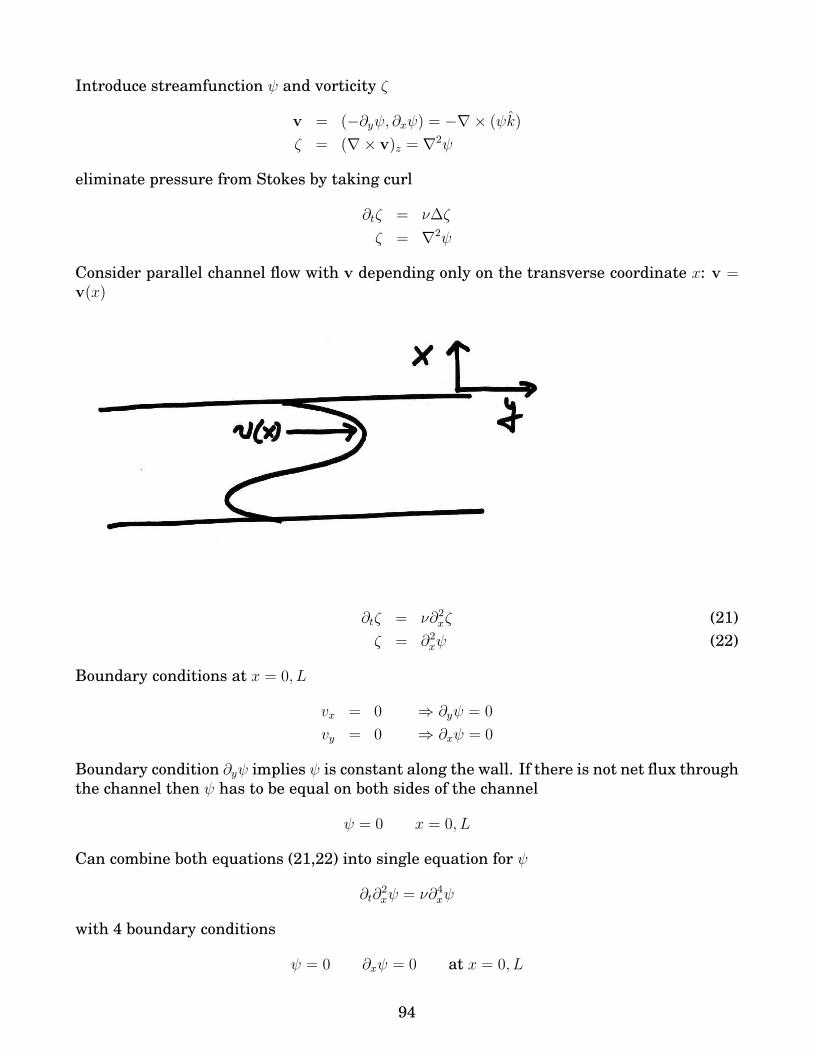
Introduce streamfunction ψ and vorticity ζ
v = (−∂yψ, ∂xψ) = −∇× (ψk)
ζ = (∇× v)z = ∇2ψ
eliminate pressure from Stokes by taking curl
∂tζ = ν∆ζ
ζ = ∇2ψ
Consider parallel channel flow with v depending only on the transverse coordinate x: v =v(x)
∂tζ = ν∂2xζ (21)
ζ = ∂2xψ (22)
Boundary conditions at x = 0, L
vx = 0 ⇒ ∂yψ = 0
vy = 0 ⇒ ∂xψ = 0
Boundary condition ∂yψ implies ψ is constant along the wall. If there is not net flux through
the channel then ψ has to be equal on both sides of the channel
ψ = 0 x = 0, L
Can combine both equations (21,22) into single equation for ψ
∂t∂2xψ = ν∂4
xψ
with 4 boundary conditions
ψ = 0 ∂xψ = 0 at x = 0, L
94
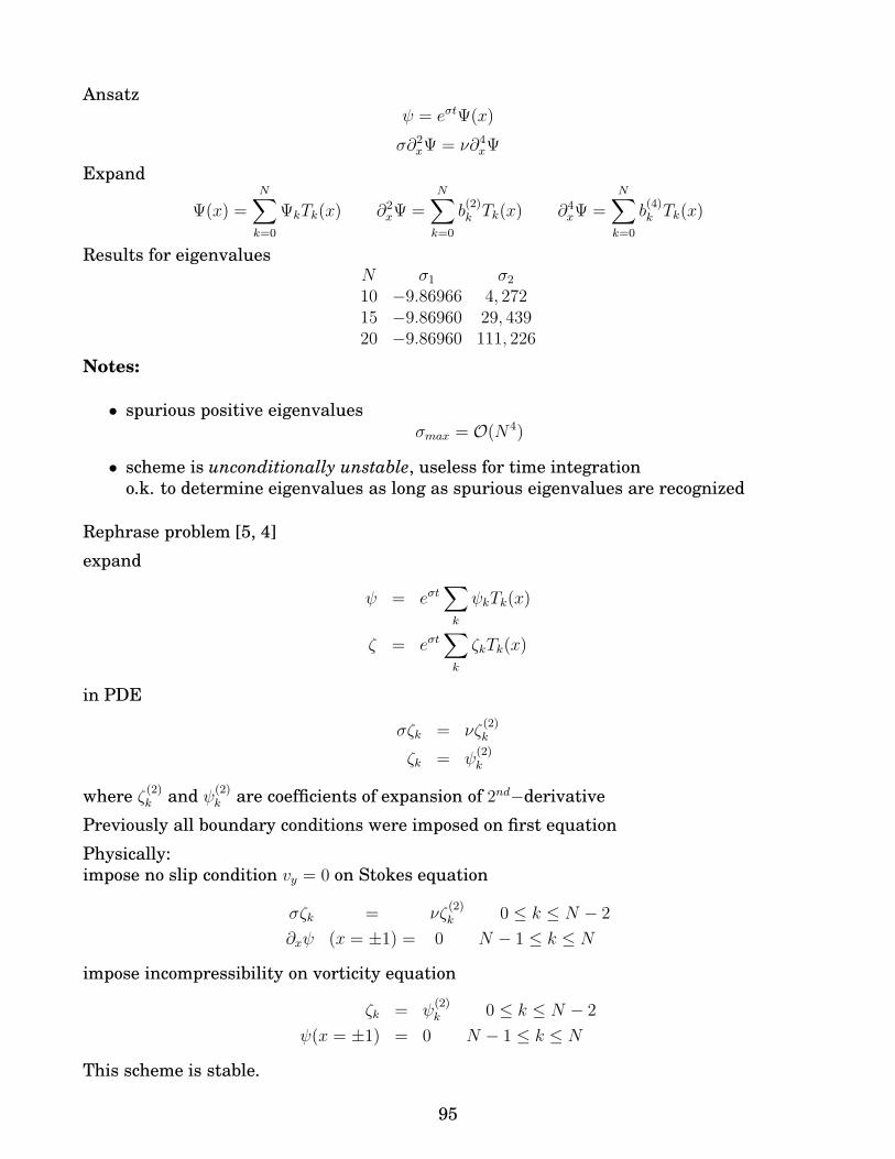
Ansatz
ψ = eσtΨ(x)
σ∂2xΨ = ν∂4
xΨ
Expand
Ψ(x) =
N∑
k=0
ΨkTk(x) ∂2xΨ =
N∑
k=0
b(2)k Tk(x) ∂4
xΨ =
N∑
k=0
b(4)k Tk(x)
Results for eigenvaluesN σ1 σ2
10 −9.86966 4, 27215 −9.86960 29, 43920 −9.86960 111, 226
Notes:
• spurious positive eigenvalues
σmax = O(N4)
• scheme is unconditionally unstable, useless for time integration
o.k. to determine eigenvalues as long as spurious eigenvalues are recognized
Rephrase problem [5, 4]
expand
ψ = eσt∑
k
ψkTk(x)
ζ = eσt∑
k
ζkTk(x)
in PDE
σζk = νζ(2)k
ζk = ψ(2)k
where ζ(2)k and ψ
(2)k are coefficients of expansion of 2nd−derivative
Previously all boundary conditions were imposed on first equation
Physically:
impose no slip condition vy = 0 on Stokes equation
σζk = νζ(2)k 0 ≤ k ≤ N − 2
∂xψ (x = ±1) = 0 N − 1 ≤ k ≤ N
impose incompressibility on vorticity equation
ζk = ψ(2)k 0 ≤ k ≤ N − 2
ψ(x = ±1) = 0 N − 1 ≤ k ≤ N
This scheme is stable.
95
9 Iterative Methods for Implicit Schemes
Consider as simple example nonlinear diffusion equation
∂tu = ∂2xu+ f(u)
with Crank-Nicholson for stability or for Newton
un+1 − un
∆t= θ∂2
xun+1 + (1 − θ)∂2
xu+ θf(un+1) + (1 − θ)f(un)
linearize f(un+1) (for reduced Newton, i.e. only single Newton step)
f(un+1) = f(un + un+1 − un) = f(un) + (un+1 − un)f ′(un) + ...
and discretize derivatives (Chebyshev or Fourier or finite differences)
∂2xu ⇒ D2u
then (
(1
∆t− θf ′(un))I − θD2
)
un+1 =
(
(1
∆t− θf ′(un))I + (1 − θ)D2
)
un + f(un)
Notes:
• in linear case matrix on l.h.s. is constant ⇒ only single matrix inversion
• in general:
– matrix inversion in each time step
– for full Newton matrix changes after each iteration
• finite differences: in one dimension only tri-diagonal matrix
• pseudospectral: matrix is full, inversion requires O(N3) operations
• implicit treatment of nonlinearity is in particular important when nonlinearity con-
tains spatial derivatives, otherwise in many cases sufficient to treat nonlinear term
explicitly (e.g. CNAB)
9.1 Simple Iteration
Goal: replace ’solving a matrix equation’ by ’multiplying by matrix’, which is faster
Consider matrix equation
Ax = b
Seek iterative solution scheme
xn+1 = xn + g(xn)
need to chose g(x) to get convergence to solution
96
xn+1 = xn ⇔ Axn = b
simplest attempt
g(x) = b− Ax
xn+1 = (I − A)xn + b ≡ Gx + b
check whether solution is a stable fixed point: consider evolution of error
δn = xn − xe
δn+1 = xn+1 − xe = (I −A)xn + b︸︷︷︸
Axe
−xe
= (I− A)(xn − xe) = (I− A)δn
thus
δn+1 = Gδn
Estimate convergence
||δn+1|| ≤ ||G|| ||δn||and
||δn|| ≤ ||G||n ||δ0||convergence in the vicinity of the solution guaranteed for
||G|| ≤ α < 1
If δn is eigenvector of G
δn+1 = Gδn = λiδn
⇒ need λi ≤ α < 1 for all eigenvalues λi
Define spectral radius of G
ρ(G) = maxi
|λi|
then we have
iteration converges iff ρ(G) ≤ α < 1
Define convergence rate R as inverse of number of iterations to decrease δ by factor e
ρ(G)1R =
1
e
R = − ln ρ(G) > 0
Note:
• for special initial conditions that lie in a direction that contracts faster one could have
faster convergence. The rate R is guaranteed.
97

• for poor initial guess: possibly no convergence at all.
For Crank-Nicholson (in the linear case)
A =1
∆tI − θD2
thus
G = I −A = (1 − 1
∆t)I + θD2
Eigenvalues of G:
ρ(G) = O(N2) Fourier
ρ(G) = O(N4) Chebyshev
ρ(G) ≫ 1 no convergence.
9.2 Richardson Iteration
Choose g(x) more carefully
g(x) = ω (b− Ax)
Iteration
xn+1 = xn + ω (b− Axn) = Gxn + ωb
with iteration matrix
G = I − ωA
Choose free parameter ω such that that ρ(G) is minimal, i.e.
maxi
|1 − ωλi| minimal
A = 1∆t
I− θD2 has only positive eigenvalues
O(1) = λmin ≤ λ ≤ λmax = O(N2,4)
98

optimal choice
1 − ωλmax = −(1 − ωλmin)
ωopt =2
λmin + λmax
optimal spectral radius
ρ(G)min = maxi
|1 − ωλi| = 1 − ωoptλmin =λmax − λmin
λmax + λmin
Spectral condition number
κ =λmax
λmin
ρ(G)min =κ− 1
κ+ 1< 1
Notes:
• Richardson iteration can be made to converge by suitable choice of ω independent of
spectral radius of original matrix
• Fourier and Chebyshev have large κ
κ = O(N2,4) ⇒ ρ very close to 1
• in Crank-Nicholson
Aij =
[1
∆t− θf ′(un)
]
δij − θD2,ij
the D2−part corresponds to calculating the second derivative ⇒ can be done using
FFT rather than matrix multiplication.
9.3 Preconditioning
Range of eigenvalues of G very large ⇒ slow convergence
Further improvement of g(x)
xn+1 = xn + ω M−1︸︷︷︸
preconditioner
(b− Axn)
Iteration matrix
G = I − ωM−1A
Goal: minimize range of eigenvalues of G
Note:
• optimal would be M−1 = A−1 then G = 0 ⇒ instant convergence
that is the original problem
• find M that is easy to invert and is close to A, i.e. has similar spectrum
⇒ use M from finite difference approximation
99
9.3.1 Periodic Boundary Conditions: Fourier
For simplicity discuss using simpler problem
∂tu = ∂2xu with periodic b.c.
backward Euler:
• spectral ⇒ A, use Fourier because of boundary conditions
• finite differences ⇒ M
Finite differences1
∆t(un+1
j − unj ) =
1
∆x2
(un+1
j+1 − 2un+1j + un+1
j−1
)
written as
Mun+1 = un
with
M =
1∆t
+ 2∆x2 − 1
∆x2 0 − 1∆x2
− 1∆x2
1∆t
+ 2∆x2
1∆x2 0
0 ... ... ...− 1
∆x2 0 − 1∆x2
1∆t
+ 2∆x2
Spectral
A =1
∆tI −D2
Eigenvalues of M−1A:
M and A have same eigenvectors eilx
⇒ eigenvalues satisfy
λM−1A =λA
λM
eigenvalues of M:
Mijeilxj =
(1
∆t− eil∆x − 2 + e−il∆x
∆x2
)
eilx
λM =1
∆t+
2
∆x2(1 − cos l∆x)
eigenvalues of A
λA =1
∆t+ l2
⇒
λM−1A =1
∆t+ l2
1∆t
+ 2∆x2 (1 − cos l∆x)
=
=∆x2
∆t+ ∆x2l2
∆x2
∆t+ 2(1 − cos l∆x)
100

range of eigenvalues
l → 0 λM−1A → 1 when∆x2
∆tdominates
l → N
2∆x2l2 →
(2π
N
N
2
)2
= π2 1 − cos l∆x→ 2 λM−1A → π2
4
Thus:
• ratio of eigenvalues is O(1) ⇒ fast convergence of iteration.
In practice
xn+1 = xn + ωM−1(b− Axn)
is solved as
M (xn+1 − xn) = ω (b −Axn)
Notes:
• for Fourier case (periodic boundary conditions) M is almost tri-diagonal , equation can
be solved fast
• for Chebyshev case: also tri-diagonal, but grid points are not equidistant, need finite
difference approximation on the same grid
∂2xu =
2
∆xj(∆xj + ∆xj−1)uj+1 −
2
∆xj∆xj−1uj +
2
∆xj−1(∆xj + ∆xj−1)uj−1 (23)
with ∆xj = xj+1 − xj
again eigenvalues of M−1A can be shown to be O(1)
• for κ ≈ 3 one has ρ = κ−1κ+1
≈ 12⇒ δn = δ12
−n
thusδnδ1
≈ 10−4 for n ≈ 12
⇒ implicit method with computational effort not much more than explicit
• the matrix multiplication should be done with fast transform, e.g. for Fourier
Axn =
(1
∆tI − D2
)
xn =1
∆txn − F−1
(−k2F(xn)
)
101

9.3.2 Non-Periodic Boundary Conditions: Chebyshev
Need to consider modified matrices, e.g. D(0,N)2 , and also in finite differences
1. fixed values u0,N = γ0,N
⇒ only N − 1 unknowns
Chebyshev: use D(0,N)2
∑
j
[δij∆t
− αD(0,N)2,ij
]
un+1j = r.h.s. +D2
i0γ0 +D2iNγN
finite differences5
1∆t
− 2α∆x2
α∆x2 0 0
α∆x2
1∆t
− 2α∆x2
α∆x2 0
0 ...0 0 α
∆x21
∆t− 2α
∆x2
=
(
r.h.s.
)
+
−1∆x2γ0
0...
−1∆x2γN
2. fixed flux ∂xu0,N = γ0,N
Chebyshev:
∂xui =∑
j
D(0,N)ij uj + δi0γ0 + δiNγN
with
D(0,N) =
0 0 0 0D
0 0 0 0
then
∂2xui =
∑
jk
DijD(0,N)jk uk
︸ ︷︷ ︸
⇒ l.h.s.
+ Di0γ0 +DiNγN︸ ︷︷ ︸
known ⇒ r.h.s.
finite differences:
introduce virtual points: u−1 and uN+1
∂xu0 =u1 − u−1
2∆x= γ0 ⇒ u−1 = u1 − 2∆xγ0
⇒ equation for u0 is modified
∂2xu0 =
u1 − 2u0 + u−1
∆x2=u1 − 2u0 + (u1 − 2∆xγ0)
∆x2
=−2
∆x2u0 +
2
∆x2u1
︸ ︷︷ ︸
l.h.s.
− 2
∆xγ0
︸ ︷︷ ︸
r.h.s.
5The matrix is actually not correct. One has to take into account the non-equidistant grid (cf. (23)).
102

M is tridiagonal
M =
1∆t
− 2∆x2
2
∆x2 0 01
∆x21
∆t− 2
∆x21
∆x2 00 ...0
Notes:
• this leads apparently to eigenvalues λM−1Ain the rangeO(1) toO( 1N
) ⇒ κ becomes
large with N , convergence not good.
• apparently better to use D(0,N)ij only to calculate derivative for the boundary points
and to calculate ∂2xu using D2 for interior points (see Streett (1983) as referenced
in [2] in Sec. 5.2)
Back to reaction-diffusion equation
∂tu = ∂2xu+ f(u)
Newton for Crank-Nicholson yields
[1
∆tI − αD2 − αI
df(un)
du
]
︸ ︷︷ ︸
A
un+1 = r.h.s.
Note:
• A depends on un ⇒ eigenvalues depend on un and therefore also on time
⇒ eigenvalues are in general not known
⇒ choice of ω is not straightforward: trial and error ‘technique’
9.3.3 First Derivative
Consider simpler problem
du
dx= f(x) with periodic b.c.
i.e. ∑
j
Dijuj = fi
Try usual central differences for finite-difference preconditioning of Fourier differentiation
matrixuj+1 − uj−1
2∆x=⇒ λM =
2i sin l∆x
2∆x
then
λM−1A =il∆x
i sin l∆xwith − π ≤ l∆x ≤ +π
since sin π = 0 one has
103

• λM−1A unbounded ⇒ κ unbounded
• no convergence
Possibilities:
1. Could omit higher modes (Orszag)
u(c)k =
{uk |k| ≤ 2N
3
0 2N3< |k| ≤ N
and calculate derivative with u(c)
duj
dx=
N∑
k=−N
iku(c)k
Now l∆x ≤ 23π and range of λM−1A is 1 ≤ λM−1A ≤ 2π
3sin 2π
3≈ 2.4.
Omitting these modes would be consistent with anti-aliasing for a quadratic nonlin-
earity.
2. Want sin 12l∆x instead of sin ∆x
Use staggered grid: evaluate derivatives and differential equation at xj+1/2 but based
on the values at the grid points xj
Finite differences
du
dx
∣∣∣∣x
j+ 12
=uj+1 − uj
∆x= e
ilxj+1
2e
12il∆x − e−
12il∆x
∆x⇒ λM =
2i sin 12l∆x
∆x
Spectral
du
dx
∣∣∣∣x
j+12
=
N∑
l=−N
ilukeil(xj+
12
πN
) ⇒ λA = il
thus
λM−1A =12l∆x
sin 12l∆x
1 ≤ λM−1A ≤ π
2
For wave equation one would get similar problem with central-difference preconditioning
λM−1A =∆x∆t
+ il∆x∆x∆t
+ i sin l∆xwith − π ≤ l∆x ≤ +π
In implicit scheme ∆t may be much larger than ∆x:again λM−1A has very large range ⇒ poor convergence
Use same method.
Note:
• one-sided difference would not have this problem either:
uj+1 − uj
∆x⇒ λM =
eil∆x
∆x
λM−1A =il∆x
eil∆x
104
10 Spectral Methods and Sturm-Liouville Problems
Spectral methods:
• expansion in complete set of functions
• which functions to choose?
To get complete set consider eigenfunctions of a Sturm-Liouville problem
d
dx
(
p(x)d
dxφ
)
− q(x)φ+ λ w(x)︸︷︷︸
weight function
φ = 0 − 1 ≤ x ≤ 1
with
p(x) > 0 in − 1 < x < 1 w(x), q(x) ≥ 0
• regular:
p(−1) 6= 0 6= p(+1)
• singular:
p(−1) = 0 and/or p(+1) = 0
Boundary conditions are homogeneous:
• regular
α±φ(±1) + β±dφ(±1)
dx= 0 (24)
• singular
p(x)dφ
dx→ 0 for x→ ±1 (25)
φ cannot become too singular near the boundary
Sturm-Liouville problems have non-zero solutions only for certain values of λ: eigenvaluesλn
Define scalar product:
〈u, v〉w =
∫ +1
−1
w(x)u∗(x)v(x)dx
eigenfunctions φk form an orthonormal complete set
〈φk, φl〉 = δlk
Examples:
105

1. p(x) = 1 = w(x) and q(x) = 0
d2
dx2φ+ λφ = 0 Fourier, regular Sturm-Liouville problem
2. p(x) =√
1 − x2, q(x) = 0, w(x) = 1√1−x2
d
dx
(√1 − x2
d
dxφ
)
+ λ1√
1 − x2φ = 0 Chebyshev, singular
Expand solutions
u(x) =∞∑
k=0
ukφk(x)
with
uk =
∫
w(x)φ∗(x)u(x) dx projection
Consider convergence of expansion in L2−norm
||u(x) −N∑
k
ukφk(x)|| → 0 for N → ∞
Note:
• pointwise convergence only for almost all x
Truncation error
||∞∑
k=N+1
ukφk(x)||
depends on decay of uk with k
Want spectral accuracy
uk ≤ O(
1
kr
)
for all r
Under what condition is spectral accuracy obtained?
Consider
uk =
∫
w(x)φ∗(x) u(x) dx
Previously (Fourier and Chebyshev) did integration by parts.
Use Sturm-Liouville problem
w(x)φ∗k(x) =
1
λk
[
qφ∗k −
d
dx
(
pdφ∗
dx
)]
106

uk
=1
λk
∫
u
{
qφ∗k −
d
dx
(
pd
dxφ∗
k
)}
dx =
=1
λk
∫
uqφ∗kdx+
1
λk
{
−up ddxφ∗
k
∣∣∣∣±1
+
∫du
dxpdφ∗
dxdx
}
=
=1
λk
∫
uqφ∗kdx+
1
λk
{
−up ddxφ∗
k
∣∣∣∣±1
+du
dxpφ∗
k
∣∣∣∣±1
−∫
d
dx
(du
dxp
)
φ∗kdx
}
Boundary terms vanish if
p
{
udφ∗
dx− du
dxφ∗
k
}∣∣∣∣±1
= 0
• regular cased
dxφ∗
k(±1) = −α±β±
φ∗k(±1)
p
{
−uα±β±
φ∗k −
du
dxφ∗
k
}∣∣∣∣±1
= 0
thus: u has to satisfy the same strict boundary conditions as φk
• singular case
pd
dxφk → 0 at boundary
⇒ require
φkpdu
dx→ 0 at boundary
need only same weak condition on u as on φ
pdu
dx→ 0 at boundary
For large k (cf. Fourier case λk = −k2 and dφk/dx = ikφk)
λk = O(k2)dφk
dx= O(k)
⇒ if boundary conditions are not met one gets
uk = O(1
k)
For spectral accuracy necessary but not sufficient:
u satisfies same boundary conditions as φ
To consider higher orders use Lφk = λkwφk to rewrite compact (cf. [2]):
uk = 〈φk, u〉w =1
λk
〈 1
wLφk, u〉w
107
if φ and u satisfy the same boundary conditions, then they are in the same function spaces
and 1wL is self-adjoint (in explicit calculation above, the w cancel and one can perform the
usual integration by parts)
uk =1
λk
〈φk,1
wLu〉w =
1
λ2k
〈 1
wLφk,
1
wLu〉w =
1
λ2k
〈φk,1
wL
1
wLu〉w
The last step can be done if 1wLu satisfies the same boundary conditions as φ.
Introducing
u(m) =1
wLu(m−1)
can write
uk =1
λrk
〈φk, u(r)〉 = O(
1
λrk
)
if
• the u(m) satisfy same boundary conditions as φ for all 0 ≤ m ≤ r − 1
• u(r) is integrable
Conclusion:
• regular Sturm-Liouville problem: since(
1wL)ru has to satisfy the boundary conditions
these boundary conditions (24) are a very restrictive condition.
Fourier case is a regular Sturm-Liouville problem: for spectral accuracy we needed
that all derivatives satisfy periodic boundary conditions.
• singular Sturm-Liouville problem: singular boundary conditions (25) only impose a
condition on regularity, do not prescribe any boundary values themselves
Simple example:
∂tu = ∂2xu+ f(x, t) u(0) = 0 = u(π)
Could use sine-series
u =∑
k
akeσt sin kx
since they satisfy related eigenvalue problem
λφ = ∂2xφ φ = 0 at x = 0, π
But: this is a regular Sturm-Liouville problem with L = ∂2x and w = 1
Spectral convergence only if
u(r)(0) = 0 = u(r)(π) for all r (26)
108

i.e. if all even derivatives have to vanish at the boundary
Most functions that satisfy the original boundary conditions u(0) = 0 = u(π) do not satisfy
the additional conditions (26)
e.g. stationary solution for f(x, t) = c
u =1
2cx2 − 1
2cπx
of course ∂2xu(x = ±1) = c 6= 0.
In fact, expanding in a sine-series one gets
ak =1
πk3
(
(−1)k − 1)
Thus:
• Expansions in natural eigenfunctions of a problem are only good if they satisfy a
singular Sturm-Liouville problem.
• If they do not satisfy a singular Sturm-Liouville problem one most likely will not get
spectral convergence even if the functions look very natural for the problem
11 Spectral Methods for Incompressible Fluid Dynam-
ics
Navier-Stokes equations for fluids arise in a wide range of application.
In many situations the fluid velocities are much smaller than the speed of sound. Density
variations can then often be assumed to propagate infinitely fast: the fluid can be assumed
to be incompressible,
∂tu + u · ∇u = −∇p + f + ν∆u
∇ · u = 0
Boundary conditions (no-slip condition and wall impermeable)
u = 0 on boundary
External forces (or imposed pressure gradients) are included in f .
The effectively infinite wave speed leads to numerical challenges.
Mathematically:
109
• pressure appears in momentum equation, but does not have an evolution equation of
its own and has no boundary condition at the walls
• divergence-free condition is an algebraic condition on the velocity, poses constraint on
the momentum equation
• could write momentum equation in terms of the vorticity ω = ∇×u
this would get rid of the pressure, but there is no convincing boundary condition for
vorticity
• divergence-free
– ⇒ can introduce streamfunction
boundary conditions can be tricky (can lead to spurious, destabilizing eigenval-
ues, cf. Sec.8.2.2)
For concreteness consider flows with boundaries only in one direction, e.g. flow between
two plates:
• 1 or 2 directions (x and z) can be approximated by periodic boundary conditions
• no-slip boundary conditions in one direction (y)
There are a number of different approaches that have been taken, we discuss only a few
selected ones. Most are formulated in terms of the primitive variables (u, p).
• coupled method: solve momentum equation and incompressibility simultaneously
• Galerkin method with divergence-free basis functions
• operator-splitting methods
Central aspects [3]:
• effectively infinite sound speed requires an implicit treatment of the pressure
• viscosity term has highest derivative: often also treated implicitly
The discussion here is following [3].
110

11.1 Coupled Method
treat u and p simultaneously in coupled equations, usually use semi-implicit method
For a first-order method one would get (with an imposed pressure gradient pxex to drive the
flow)
1
∆tun+1 − ν∆un+1 + ∇pn+1 = fn+1 + pxex +
1
∆tun − un · ∇un (27)
∇ · un+1 = 0
un+1 = 0 on boundary
Derivatives implemented via ik in the x-direction and via Chebyshev differentiation matrix
in y-direction:
u =∑
Uk(y, t)eikx =
∑
Ukm(t)Tm(y)eikx p =∑
Pk(y, t)eikx =
∑
Pkm(t)Tm(y)eikx (28)
With (28) and U = (U, V ) the Navier-Stokes equation (27) becomes
1
∆tUn+1
k + νk2Un+1k − ν∂2
yUn+1k + ikP n+1
k ex + ∂yPn+1k ey = rk (29)
ikUn+1k + ∂yV
n+1k = 0
with
rk =1
∆tUn
k − (un · ∇un)k − (pxex)k (30)
and boundary condition
Un+1k (y = ±1) = 0
System can be solved
• directly with iterative method (precondition for the y-derivative)
• using the influence matrix method (Kleiser-Schumann)
Discuss here the influence matrix method.
For U one gets from (29)
−νU ′′ + λU + ikP = rx (31)
with
U(y = ±1) = 0
and
λ =1
∆t+ νk2.
For V one gets
−νV ′′ + λV + P ′ = ry (32)
with boundary condition
V (y = ±1) = 0. (33)
111

Once P is known U and V can be determined from (31, 32).
To get an equation for the pressure eliminate Un+1 from (27) by taking its divergence and
using incompressibility (drop subscript k and superscript n = 1)
P ′′ − k2P = ∇ · r (34)
We do not have a boundary condition for the pressure. Instead, using ∇ · U = 0 and
∂xU(y = ±1) = 0 one gets the boundary condition on V ′
V ′(y = ±1) = 0 (35)
Thus, the P -equation is coupled to the V -equation through this additional boundary condi-
tions. Need to compute P and V simultaneously using (34,35,32,33)
L(PV
)
= b V (y = ±1) = 0 = V ′(y = ±1) (36)
with
L =
(∂2
y − k2 0−∂y ν∂2
y − λ
)
b =
(∇ · r−ry
)
Slightly strange boundary conditions:
• 2nd-order ODE for P but no boundary condition for P
• 2nd-order ODE for V but 4 boundary conditions for V
Consider auxiliary problem, assuming there is a boundary condition for P ,
L(PV
)
= b P (y = ±1) = P± V (y = ±1) = 0 (37)
(36) can be solved by solving 3 versions of (37):
L(Pp
Vp
)
= b Pp(y = ±1) = 0 Vp(y = ±1) = 0 (38)
L(P+
V+
)
= 0 P+(y = +1) = 1 P+(y = −1) = 0 V+(y = ±1) = 0 (39)
L(P−V−
)
= 0 P−(y = +1) = 0 P−(y = −1) = 1 V−(y = ±1) = 0 (40)
Expand the solution to (36) as(PV
)
=
(Pp
Vp
)
+ δ+
(P+
V+
)
+ δ−
(P−V−
)
(41)
and impose the boundary condition of (36)(V ′
+(+1) V ′−(+1)
V ′+(−1) V ′
−(−1)
)
︸ ︷︷ ︸
M
(δ+δ−
)
= −(V ′
p(+1)V ′
p(−1)
)
Since L does not depend on the flow (U, P ) the solutions to (39) and to (40) do not depend
on the flow:
112
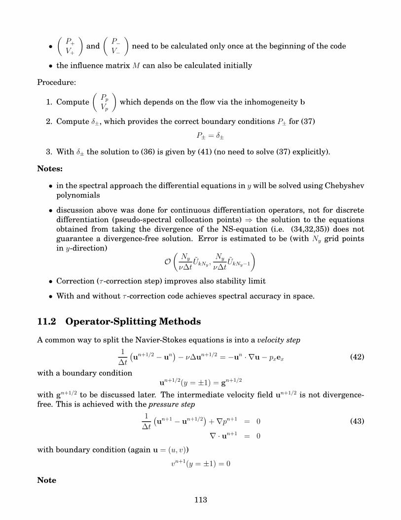
•(P+
V+
)
and
(P−V−
)
need to be calculated only once at the beginning of the code
• the influence matrixM can also be calculated initially
Procedure:
1. Compute
(Pp
Vp
)
which depends on the flow via the inhomogeneity b
2. Compute δ±, which provides the correct boundary conditions P± for (37)
P± = δ±
3. With δ± the solution to (36) is given by (41) (no need to solve (37) explicitly).
Notes:
• in the spectral approach the differential equations in y will be solved using Chebyshev
polynomials
• discussion above was done for continuous differentiation operators, not for discrete
differentiation (pseudo-spectral collocation points) ⇒ the solution to the equations
obtained from taking the divergence of the NS-equation (i.e. (34,32,35)) does not
guarantee a divergence-free solution. Error is estimated to be (with Ny grid points
in y-direction)
O(Ny
ν∆tUkNy
,Ny
ν∆tUkNy−1
)
• Correction (τ -correction step) improves also stability limit
• With and without τ -correction code achieves spectral accuracy in space.
11.2 Operator-Splitting Methods
A common way to split the Navier-Stokes equations is into a velocity step
1
∆t
(un+1/2 − un
)− ν∆un+1/2 = −un · ∇u− pxex (42)
with a boundary condition
un+1/2(y = ±1) = gn+1/2
with gn+1/2 to be discussed later. The intermediate velocity field un+1/2 is not divergence-
free. This is achieved with the pressure step
1
∆t
(un+1 − un+1/2
)+ ∇pn+1 = 0 (43)
∇ · un+1 = 0
with boundary condition (again u = (u, v))
vn+1(y = ±1) = 0
Note
113
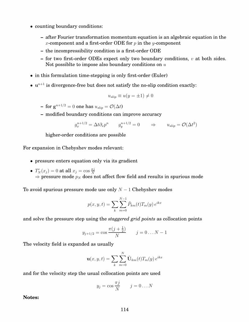
• counting boundary conditions:
– after Fourier transformation momentum equation is an algebraic equation in the
x-component and a first-order ODE for p in the y-component
– the incompressibility condition is a first-order ODE
– for two first-order ODEs expect only two boundary conditions, v at both sides.
Not possiblte to impose also boundary conditions on u
• in this formulation time-stepping is only first-order (Euler)
• un+1 is divergence-free but does not satisfy the no-slip condition exactly:
uslip ≡ u(y = ±1) 6= 0
– for gn+1/2 = 0 one has uslip = O(∆t)
– modified boundary conditions can improve accuracy
gn+1/2x = ∆t∂xp
n gn+1/2y = 0 ⇒ uslip = O(∆t2)
higher-order conditions are possible
For expansion in Chebyshev modes relevant:
• pressure enters equation only via its gradient
• T ′N (xj) = 0 at all xj = cos πj
N
⇒ pressure mode pN does not affect flow field and results in spurious mode
To avoid spurious pressure mode use only N − 1 Chebyshev modes
p(x, y, t) =∑
k
N−1∑
m=0
Pkm(t)Tm(y) eikx
and solve the pressure step using the staggered grid points as collocation points
yj+1/2 = cosπ(j + 1
2)
Nj = 0 . . . N − 1
The velocity field is expanded as usually
u(x, y, t) =∑
k
N∑
m=0
Ukm(t)Tm(y) eikx
and for the velocity step the usual collocation points are used
yj = cosπj
Nj = 0 . . . N
Notes:
114

• The pressure mode P00 also does not affect the flow. However, a spatially homogeneous
pressures is also physically irrelevant⇒ indeterminacy of P00 does not pose a problem.
• Since two different grids are used one needs to interpolate (u, p) from one grid to the
other by evaluating the Tm at the respective grid points. This introduces additional
steps in the algorithm (some slowing down).
Velocity Step
drop again subscript k
ν∂2yU
n+1/2 − λUn+1/2 = −r
Un+1/2(y = ±1) = gn+1/2(y = ±1)
with λ = 1∆t
+ νk2 and r as in (30)
Determine U using Chebyshev τ -method using the usual (Gauss-Lobatto) collocation points
yj .
Pressure Step
For transformation between the grids write
U = (U(y0), U(y1), . . . , U(yN))t V = (V (y0), V (y1), . . . , V (yN))t
and
P =(P (y1/2), P (y3/2), . . . , P (yN−1/2)
)t
Need to compute the Chebyshev coefficients U and P for U and P based on the values at
the respective grid points
U = C0U V = C0V
and
P = C+P
where C0 and C+ are the appropriate matrices
Velocity divergence needed on staggered grid points
∇ · u → DU ≡(C−1
+ C0
) [
ikU + C−10 DC0V
]
where D computes the derivative from the Chebyshev coefficients
Pressure gradient needed on regular grid points in momentum equation
∇p→ GP ≡(C−1
0 C+
) (
ikP ,C−1+ DC+P
)
Pressure step (43) becomes
Un+1 = Un+1/2 − ∆tGP at interior points yj, j = 1 . . .N − 1 (44)
DUn+1 = 0 at yj+1/2, j = 0 . . . N − 1 (45)
115
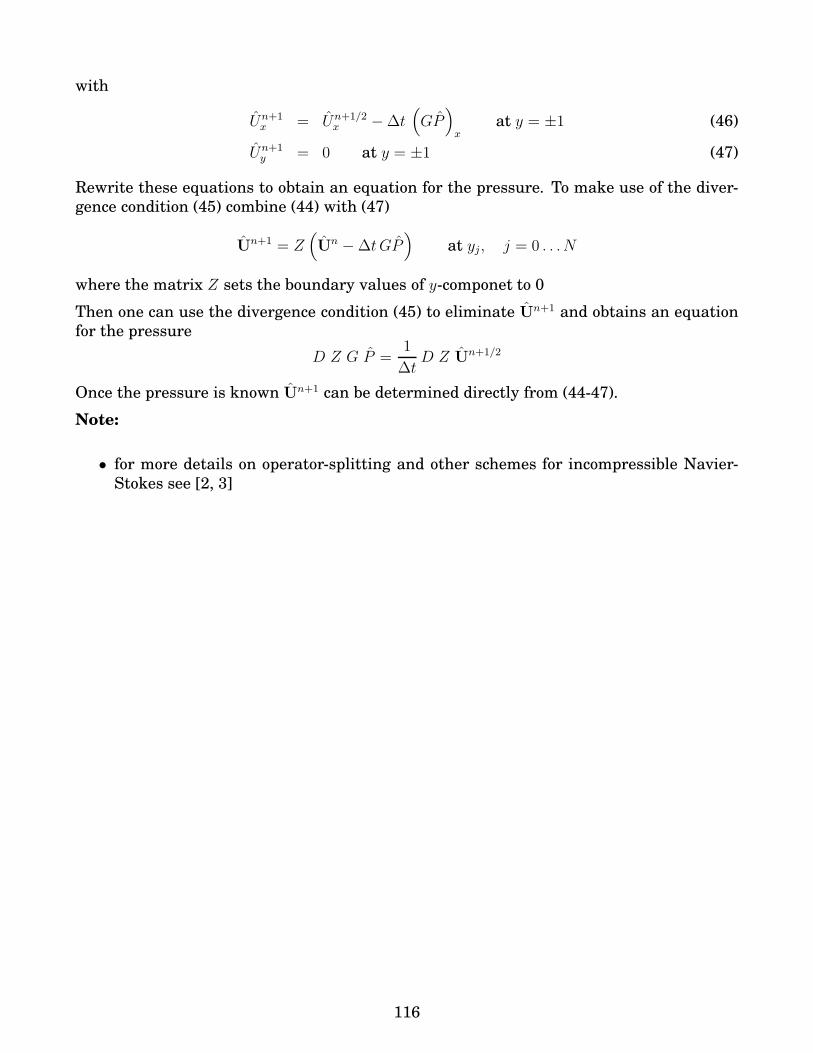
with
Un+1x = Un+1/2
x − ∆t(
GP)
xat y = ±1 (46)
Un+1y = 0 at y = ±1 (47)
Rewrite these equations to obtain an equation for the pressure. To make use of the diver-
gence condition (45) combine (44) with (47)
Un+1 = Z(
Un − ∆tGP)
at yj, j = 0 . . . N
where the matrix Z sets the boundary values of y-componet to 0
Then one can use the divergence condition (45) to eliminate Un+1 and obtains an equation
for the pressure
D Z G P =1
∆tD Z Un+1/2
Once the pressure is known Un+1 can be determined directly from (44-47).
Note:
• for more details on operator-splitting and other schemes for incompressible Navier-
Stokes see [2, 3]
116
A Insertion: Testing of Codes
A few suggestions for how to test codes and identify bugs:
• test each term individually if possible
– set all but one coefficient in the equation to 0:
does the code behave qualitatively as expected from the equation?
– compare quantitatively with simple analytical solutions (possibly with some co-
efficients set to 0)
• code ‘blows up’:
– is it a ‘true blow-up’: exact solution should not blow up
– is the blow-up reasonable for this type of scheme for this problem? Stability?
Does decreasing dt increase/decrease the growth?
– is the blow-up a coding error?
• track variables:
use only few modes so you can print out/plot what is going on in each time step
• if the code seems not to do what it should it often is a good idea to vary the parameters
and see whether the behavior of the code changes as expected (e.g. if a parameter was
omitted in an expression the results may not change at all even though the parame-
ters are changed); the response of the code to parameter changes may give an idea for
where the error lies.
B Details on Integrating Factor Scheme IFRK4
Some more details for the integrating-factor scheme (keeping in mind that it is usually not
as good as the exponential time differencing scheme):
Rewrite (8) with integrating factor ek2t
∂t(ek2tuk) = k2ek2tuk + ek2t∂tuk = ek2tfk(u) (48)
Introduce auxiliary variable vk(t) = ek2tuk(t)
∂tvk = ek2tfk(e−l2tvl) (49)
Note:
• for nonlinear f the Fourier coefficient fk depends on all Fourier modes of v
117

It is natural to consider now suitable time-integration methods to solve equation (49)
Example: Forward Euler
vn+1k = vn
k + ∆t ek2tfk(e−k2tvn
k )
ek2(t+∆t)un+1k = ek2tun
k + ∆t ek2tfk(unk)
un+1k = e−k2∆t (un
k + ∆t fk(unk))
Note:
• with forward Euler integrating factor generates same scheme as the operator-splitting
scheme above
• diffusion and other linear terms are treated exactly
• no instability arises from linear term for any ∆t
• large wave numbers are strongly damped, as they should be (this is also true for
operator splitting)
compare with Crank-Nicholson (in CNAB, say)
un+1k =
1 − 12∆tk2
1 + 12∆tk2
unk
for large k∆t
un+1k = −(1 − 4
∆tk2+ ...)un
k
oscillatory behavior and slow decay.
• FFT is done on nonlinear term rather than the linear derivative term (cf. operator
splitting)
• But: fixed points in u depend on the time step ∆t and are not computed correctly
for large ∆t, whereas without the integrating factor the fixed points of the numerical
scheme agree exactly with those of the differential equation.
Notes:
• It turns out that the prefactor of the error term is relatively large in particular com-
pared to the exponential time differencing scheme (cf. Boyd, Chebyshev and Fourier
Spectral Methods6)
Details for Runge-Kutta:
In Fourier space
∂tuk = −k2uk + fk(u)
6See also Cox and Matthews, J. Comp. Phys. 176 (2002) 430, who give a detailed comparison and a further
advanced method exponential time differencing.
118

For vk = ek2tuk then
∂tvk = ek2tfk(vle−l2t) = Fk(t, vl)
Note: Fk(t, vl) depends explicitly on time even if f(u) does not!
Then
k1k = ∆tFk(tn, vnl ) =
= ∆t ek2tnfk(vnl e
−l2tn) = ∆tek2tnfk(unl )
k2k = ∆tFk(tn +1
2∆t, vn
l +1
2k1l) =
= ∆t ek2(tn+∆t/2)fk((vnl +
1
2k1l) e
−l2(tn+∆t/2))
= ∆t ek2(tn+∆t/2)fk(vnl e
−l2tne−l2∆t/2 +1
2k1le
−l2(tn+∆t/2))
= ∆t ek2(tn+∆t/2)fk(unl e
−l2∆t/2 +1
2k1le
−l2(tn+∆t/2))
Growing exponentials become very large for large k. Introduce
k1k = k1ke−k2tn
k2k = k2ke−k2(tn+∆t/2)
k3k = k3ke−k2(tn+∆t/2)
k4k = k4ke−k2(tn+∆t)
Then
k1k = ∆t fk(unl )
k2k = ∆t fk(unl e
−l2∆t/2 +1
2k1le
−l2∆t/2)
= ∆t fk
(
(unl +
1
2k1l)e
−l2∆t/2
)
k3k = ∆t fk
(
unl e
−l2∆t/2 +1
2k2l
)
k4k = ∆t fk
(
unl e
−l2∆t + k3le−l2∆t/2
)
vn+1k = vn
k +1
6(k1k + 2k2k + 2k3k + k4k)
un+1k ek2(tn+∆t) = un
kek2tn +
1
6ek2tn
(
k1k + 2k2kek2∆t/2 + 2k3ke
k2∆t/2 + k4kek2∆t
)
Thus
un+1k = un
ke−k2∆t +
1
6
(
k1ke−k2∆t + 2k2ke
−k2∆t/2 + 2k3ke−k2∆t/2 + k4k
)
Note
• In each of the four stages go to real space to evaluate nonlinearity and then transfrom
back to Fourier space to get its Fourier components in order to evaluate kik, i = 1..4.
119
C Chebyshev Example: Directional Sensing in Chemo-
taxis
Levine, Kessler, and Rappel have introduced a model to explain the ability of amoebae (e.g.
Dictyostelium discoideum) to sense chemical gradients very sensitively despite the small
size of the amoeba (see PNAS 103 (2006) 9761).
The model consists of an activator A, which is generated in response to the external chem-
ical that is to be sensed. The activator is bound to the cell membrane and constitutes the
output of the sensing activity (and triggers chemotactic motion), and a diffusing inhibitor
B. The inhibitor can attach itself to the membrane (its concentration is denoted Bm) where
it can inactivate A.
The model is given by
∂B
∂t= D∇2B inside the cell − 1 < x < +1
with boundary ocndition
D∂B
∂n= kaS − kbB.
Here ∂/∂n is the outward normal derivative. In a one-dimension system its sign is opposite
on the two sides of the system, ∂/∂n = −∂/∂x at x = −1 whereas ∂/∂n = +∂/∂x at x = +1 .
The reactions of the membrane bound species are given by
dA
dt= kaS − k−aA− kiABm
dBm
dt= kbB − k−bBm − kiABm
To implement the boundary conditions with Chebyshev polynomials (using the matrix mul-
tiplication approach):
∂Bi
∂x=
N∑
j=0
DijBj for i = 1, . . . , N − 1
∂B0
∂x= − 1
D(kaS0 − kbB0)
∂BN
∂x=
1
D(kaSN − kbBN)
The second derivative is then given by
D∂2Bi
∂x2= D
N−1∑
j=1
N∑
k=0
DijDjkBk −Di0 (kaS0 − kbB0) +DiN (kaSN − kbBN)
which can be written as
D∂2Bi
∂x2=
N∑
k=0
DikBk + ka (−Di0S0 +DiNSN)
120
with
Dik = DN−1∑
j=1
DijDjk − b
−Di0 0 0 DiN
−Di0 ... ... DiN
−Di0 ... ... DiN
−Di0 0 0 DiN
The equations on the membrane are nonlinear. The implementation of Crank-Nicholson
is then done most easily not completely implicitly, i.e. no full Newton iteration sequence
is performed to solve the nonlinear equations. Instead only a single iteration is performed
(semi-implicit) This is equivalent to expanding the terms at the new time around those at
the old time. Specifically
αAn+1Bn+1 + (1 − α)AnBn = α ((An + ∆A)(Bn + ∆B)) + (1 − α)AnBn =
= α (AnBn + An∆B +Bn∆A + O(∆A∆B)) + (1 − α)AnBn =
= α(An+1Bn + AnBn+1
)+ (1 − 2α)AnBn + O(∆A∆B).
Ignoring the term O(∆A∆B) is often good enough.
D Background for Homework: Transitions in Reaction-
Diffusion Systems
Many systems undergo transitions from steady state to oscillatory ones or from spatially
homogeneous ones to states with spatial structure (periodic or more complex)
Examples:
• buckling of a bar or plate upon uniform compression (Euler instability)
• convection of a fluid heated from below: thermal instability through bouyancy or
temperature-dependence of surface tension
• fluid between two rotating concentric cylinders: centrifual instability
• solid films adsorbed on substrates with different crystaline structure (cf. Golovin’s
recent coloquium)
• surface waves on a vertically vibrated liquid
• various chemical reactions: Belousov-Zhabotinsky
– oscillations:
in the 1950s Belousov could not get his observations published because the jour-
nal reviewers thought such temporal structures were not ‘allowed’ by the second
law of thermodynamics
– spatial structure:
Turing suggested (1952) that different diffusion rates of competing chemicals
could lead to spatial structures that could underly the formation of spatial struc-
tures in biology (segmentation of yellow-jackets, patterning of animal coats...)
121

Common to these systems is that the temporal or spatial structures arise through instabil-
ities of a simpler (e.g. homogeneous) state. Mathematically, these instabilities are bifurca-
tions at which new solutions come into existence.
General analytical approach:
1. find simpler basic state
2. identify instabilities of basic state
3. derive simplified equations that describe the structured state in the weakly nonlinear
regime
leads to equations for the amplitude of the unstable modes characterizing the struc-
ture: Ginzburg-Landau equations
In homework consider simple model in one spatial dimension for chemical reaction involv-
ing two species
∂tu = D1∂2xu+ f(u, v)
∂tv = D2∂2xu+ g(u, v)
‘Brusselator’ (introduced by Glansdorff and Prigogine, 1971, from Brussels) does not model
any specific reaction, it is just s very simple rich model
f(u, v) = A− (B + 1) u+ u2v
g(u, v) = Bu− u2v
with A and B external control parameters. Keep in the following A fixed and vary B.
For all parameter values there is a simple homogeneous steady state
u = A v =B
A
This state may not be stable for all values of B: study stability by considering small pertur-
bations
u = A+ U
v =B
A+ V
Inserting in original equation
u2v = AB + 2BU + A2V + U2B
A+ 2AUV + U2V
∂tU = D1∂2xU + (B − 1)U + A2V + F (U, V )
∂tV = D2∂2xV − BU − A2V − F (U, V )
with
F (U, V ) =B
AU2 + 2AUV + U2V
122

Linear stability: omit F (U, V ), which is negligible for infinitesimal U and V
(∂tU∂tV
)
=
(D1∂
2xU
D2∂2xV
)
+
(B − 1 A2
−B −A2
)
︸ ︷︷ ︸
M0
(UV
)
Exponential ansatz (UV
)
= eσteiqxA(U0
V0
)
(50)
M(σ, q)
(U0
V0
)
≡(
−σ −D1q2 +B − 1 A2
−B −σ −D2q2 − A2
)(U0
V0
)
= 0
has only a solution if
detM(σ, q) = 0
σ2 + σ((D1 +D2)q
2 + A2 − B + 1)
︸ ︷︷ ︸
α(q)
+A2(B − 1) + q2(A2D1 + (1 −B)D2
)+D1D2q
4
︸ ︷︷ ︸
β(q)
= 0
This gives a relation
σ = σ(q)
Instability occurs if
ℜ(σ) ≡ σr > 0 for some q
In this model two possibilities for onset of instability
• σ = iω with q = 0: oscillatory instability leading to Hopf bifurcation
expect oscillations to arise with frequency ωoccurs for α(q = 0) = 0
B(H)c = 1 + A2 ωc = σi
• σ = 0 with q 6= 0: instability sets in first at a specific q = qc (critical wavenumber)
expect spatial structure to arise with wavenumber qcoccurs for β(qc) = 0
B(T )c =
(
1 + A
√
D1
D2
)2
q2c =
A√D1D2
here used σ(qc, B(T )c ) = 0 as well as dσ
dq
∣∣∣qc,B
(T )c
= 0 to get the value where the first mode
becomes unstable.
For small amplitude A one can do a weakly nonlinear analysis, expanding the equations in
A and B − B(H,T )c to obtain a Ginzburg-Landau equation for the complex amplitude A,
∂TA = δ ∂2XA + µA− γ|A|2A
For Hopf bifurcation δ, µ, and γ are complex, for Turing bifurcation they are real.
123
In the original exponential ansatz (50) amplitude A is constant. It turns out one can al-
low A allow to vary slowly in space and time. The Ginzburg-Landau equation has simple
spatially/temporally periodic solutions
A = A0eiωteiqx
with
A20 =
µr − δrq2
γr
ω = µi − δiq2 − γi|A|2
This leads to solutions for U and V of the form(UV
)
= ei(ωc+ω)tei(qc+q)xA0
(U0
V0
)
+ h.o.t.
In the homework the system has non-trivial boundaries: affects the onset of the instabil-
ities. In this case one gets interesting behavior already for values of B that are slightly
below Bc. Instabilities can arise at boundaries, which then can interact with the instabili-
ties in the interior of the system.
E Background for Homework: Pulsating Combustion
Fronts
Consider a one-dimensional combustible fluid in which the reactants are well mixed (pre-
mixed) and in which the concentration of a rate-limiting reactant is given by Y . The temper-
ature of the fluid is given by T . A simple reaction with Arrhenius kinetics is then described
by
∂tT = κ∂2xt+ q Y k(T )
∂tY = D∂2xY − Y k(T )
with the reaction term
k(T ) = k0e− E
kBT
with E the activation energy and kB the Boltzmann constant.
Boundary conditions
T (0, t) = Tl T (L, t) = Tr
Y (0, t) = Yl Y (L, t) = Yr
and initial conditions
T (x, 0) = T0 Y (x, 0) = Y0
Make dimensionless
C =Y
Y0
and
θ =T − Tad
Tad − T0Tad = T0 + qY0
124

i.e.
T = Ta + qY0θ
Insert into Arrhenius law
e−E/kBT = e−E/kBTaeE/kB(1/Ta−1/T )
= k(Ta)exp
(E
kB
1
TaT(T − Ta)
)
= k(Ta)exp
(E
kBTa
qY0θ
Ta + qY0θ
)
= k(Ta)exp
(Zθ
1 + δθ
)
with the Zeldovich number Z given by
Z =E
kBTa
qY0
Ta
and δ =qY0
Ta
This results in the final equations
∂tθ = ∂2xθ + Ce
Zθ1+δθ (51)
∂tC =1
Le∂2
xC − CeZθ
1+δθ (52)
with Lewis number given by
Le =κ
D
Initial conditions
C = 1 θ = −1
and boundary conditions
θ = θl,r C = Cl,r
For very large activation energy (Z large) the reaction front can be replaced by an internal
layer and one can treat the outer solution analytically. A linear stability analysis shows
that for Le > 1 and the Zeldovich number above a certain value of Zc(Le) the steadily
propagating front becomes unstable to oscillations and a transition to pulsating fronts occur
[8]. In two-dimensional versions of (51,52) instabilities to cellular flames arise for Le < 1(cf. Fig. 7).
125

Figure 7: Cellular flame on a porous plug burner (from http://vip.cs.utsa.edu/flames/overview.html see also [9]).
126


![Hermann Riecke - Physics Courses · 2018-09-27 · Stochastic differential equations: theory and applications. Wiley, New York, 1974 ... Science, 276(5314):917–922, May 1997. [3]](https://static.documents.pub/doc/80x56/5f0b8d967e708231d4311520/hermann-riecke-physics-courses-2018-09-27-stochastic-differential-equations.jpg)
