HestonStochastic VolatilityModel of Stock Prices

Peter Deeney

Project Supervisor

Dr Olaf Menkens

School of Mathematical Sciences

Dublin City University

August 2009

Declaration

I hereby certify that this material, which I now submit for assessment on the

programme of study leading to the award of Master of Science in Financial and

Industrial Mathematics, is entirely my own work and has not been taken from the

work of others save and to the extent that such work has been cited and acknowl-

edged within the text of my work.

Signed

Student No 58211432

26th August 2009

1

Acknowledgements

I would like to thank Dr Menkens and Dr Forde for their assistance, I would

also like to thank the staff of the DCU Library.

2

Contents

1 Introduction 6

1.1 Basic Introduction to Options . . . . . . . . . . . . . . . . . . . . . 6

1.2 Ito’s Lemma and Stochastic Processes . . . . . . . . . . . . . . . . . 7

1.3 Put Call Parity for European Options . . . . . . . . . . . . . . . . . 8

2 Constant Volatility Model (CV) 10

2.1 Black Scholes Merton (BSM) Formula for Option Prices . . . . . . . 11

2.2 Comparison with Empirical Data . . . . . . . . . . . . . . . . . . . 13

3 Stochastic Volatility (SV) 18

3.1 Derivation of the Dupire Eqn for Local Volatility . . . . . . . . . . 23

3.2 Local Variance in Terms of Instantaneous Variance . . . . . . . . . 26

4 Heston Model 29

4.1 An Explicit Solution . . . . . . . . . . . . . . . . . . . . . . . . . . 30

4.2 A Complex Logarithm Conjecture . . . . . . . . . . . . . . . . . . . 36

4.3 Numerical Integration . . . . . . . . . . . . . . . . . . . . . . . . . 37

4.4 Monte Carlo Simulation using Milstein Discretization . . . . . . . . 40

4.5 The Predicted Implied Volatility Surface . . . . . . . . . . . . . . . 44

4.6 SVI Model . . . . . . . . . . . . . . . . . . . . . . . . . . . . . . . . 48

4.7 Estimation of the Heston Parameters . . . . . . . . . . . . . . . . . 48

4.8 Remarks Concerning the Heston Model . . . . . . . . . . . . . . . . 50

5 Further Developments, Jump Diffusion Model and SABR 52

5.1 Stochastic Volatililty with Jumps (SVJ) . . . . . . . . . . . . . . . 52

3

5.2 Stochastic α, β, ρ (SABR) . . . . . . . . . . . . . . . . . . . . . . . 53

6 Conclusion 55

A Numerical Integration 57

A.1 Matlab Code for Explicit Solution . . . . . . . . . . . . . . . . . . . 57

A.2 Programmes Supporting Reliability of the Explicit Solution . . . . . 59

B Monte Carlo Milstein Discretization 60

4

Abstract

There are problems with the usual assumption of a log normal distri-

bution of stock prices, the most important discrepancy is to be found in

the tails and in time dependent volatility. To get a more accurate model of

the distribution of stock prices one suggestion is to use a stochastic volatil-

ity (SV) model. This project concentrates on Heston’s stochastic volatility

model. This provides a very useful way to price exotic options based on

the prices for plain vanillas. Heston’s model is particularly useful as it is

possible to find explicit formulas for the distribution of prices for Heston’s

SV model. Further improvements are mentioned namely adding jumps to

the stochastic volatility model, (SVJ) and the SABR model.

5

1 Introduction

1.1 Basic Introduction to Options

Consider the following example. We do not know how much oil will cost in 12

months, and yet many businesses need to plan ahead and sign contracts, this

requires some assumptions about the unknown price in a year’s time. One way to

avoid nasty surprises is to agree a price now which will be paid in 12 months when

the oil is delivered. This is called a forward contract. In a forward contract no

money changes hands at the start and the two parties agree the price of an item

to be delivered at some specified date in the future.

There is still a problem. We know how foolish we would feel if it turned out

that we had agreed to pay a higher price than we could have paid on the open

market. Wouldn’t it be good to have the means to know in advance whether to

take the forward price or the market price? This is the reason options are so useful,

they allow us to select a price in advance, known as the strike price, and make

the choice whether to trade at this price when we find out the market price on

the expiry date. Such a choice isn’t free. One party usually pays the other some

money initially in order to enter the contract. How much should such an option

cost? Naturally in the absence of a time machine we do not know the future price

of oil or of any other risky asset. We can however make intelligent guesses as to the

likely outcomes. That is, we can postulate models of the probability distribution

and use these to price the options. We concern ourselves only with options which

are only able to be exercised on their expiry date, these are known as European

options. We do not deal with American options which can be exercised at times

before their expiry date.

6

Section 2 deals with the Black Scholes Merton model of asset prices which as-

sumes constant volatility (CV). This model is compared with empirical results. An

improvement to this model is then proposed in Section 3, the Stochastic Volatility

model (SV), and some general properties of this are found. The Heston model is

a particular version of the SV model and it is examined in some detail in Section

4. Some other models notably the Jump Diffusion model (SVJ) and SABR mod-

els are mentioned in Section 5. There is a short conclusion in Section 6 and the

appendices contain the Matlab and Maple code used in the calculations.

1.2 Ito’s Lemma and Stochastic Processes

Use is made of Ito’s Lemma in this report, we begin with a brief description of a

Stochastic Process. Let (Ω, F, T ) be a probability space. A stochastic process is a

set of random variables St|t ∈ [0, T ] defined on (Ω, F, T ).

For our purposes the random variables will take values on the Real numbers,

and in many cases the positive Reals. We cannot predict future values of a random

variable, St, but if we know the distribution of the stochastic process we may

calculate the probability of various outcomes. There are equations which try to

model the rates of change of deterministic and stochastic variables. Ito calculus

provides the extension of regular calculus to stochastic variables so that we may

make use of such ideas. The basic statement of Ito’s Lemma for f ∈ C1,2 and a

stochastic process S, is

df =δf

δtdt+

δf

δSdS +

1

2

δ2f

δS2(dS)2. (1.1)

The multiplication rules for W1 and W2, two standard Brownian motions with

7

correlation ρ, are shown in Table 1.1 on page 8.

Product dt dW1 dW2

dt 0 0 0

dW1 0 dt ρdt

dW2 0 ρdt dt

Table 1.1: Multiplication table for Ito products.

The Lemma allows us to understand the interaction of stochastic and normal

calculus. That is, it allows us to define an integral over a stochastic variable which

is compatible with our definitions for deterministic variables.

It is more formally expressed in integral form:

ˆdf =

ˆδf

δtdt+

ˆδf

δSdS +

ˆ1

2

δ2f

δS2(dS)2.

If f depends on two stochastic processes, X and Y , we use the following:

df =δf

δtdt+

δf

δXdX +

1

2

δ2f

δX2(dX)2 +

δf

δYdY +

1

2

δ2f

δY 2(dY )2 +

1

2

δ2f

δXδY. (1.2)

This is applied in (3.6).

1.3 Put Call Parity for European Options

A call option is the right to buy the underlying asset for the strike price, K at the

expiry time, T . A put option is the right to sell the underlying asset for the strike

price K at the expiry time T . There is of course, a relationship between the value

of the call and put option, which is known as put call parity. It is common practice

to evaluate call options and use put call parity to calculate put option prices from

8

the call option prices. We will do this in the explicit solution calculations in table

2.1.

A portfolio consisting of a call option and cash equal to the present value of K,

has the same value at expiration as a portfolio of a put option and the underlying

asset. To see this, consider the first portfolio, a call option and cash which will be

worth K at expiry; this portfolio will be worth the maximum of K or the stock it

can purchase. At expiry the second portfolio is worth the maximum of the stock

price or K, because you have the right to sell the stock for K. Since both are

worth the same at expiry and we assume there is no arbitrage, (risk free profit),

then they are worth the same at the start. Let

K, be the strike price,

S, be the present value of the risky asset,

T , be the time gap from now to expiry,

r, be the risk free rate of interest with continuous compounding,

P , be the value of a put option and

C, be the value of a call option, then the following holds:

C +Ke−rT = P + S. (1.3)

9

2 Constant Volatility Model (CV)

The classical model of stock prices is known as the Black Scholes Merton model,

it was published in 1973. It assumes that the volatility is constant. Thus the

dynamics of the prices of risky assets can be modelled by geometric Brownian

motions (2.1). This leads to a distribution which is lognormal. The following

notation will be used:

St is the value of the risky asset at time t, (stock, commodity or other security),

r is the risk free interest rate,

Wt is a standard Brownian motion with zero mean and variance t and,

σ is the constant volatility. Then the price dynamics is given by

dSt = rStdt+ σStdWt. (2.1)

It is possible to calculate prices of derivatives within this model. A derivative

is a financial contract whose value is a function of the value of an underlying asset.

In particular we are interested in options but there are other kinds of derivatives.

In order to derive the price of a derivative, let us consider a portfolio which has a

value of Π, and is composed of of minus one derivative, and δfδS

units of risky asset,

where f(S) is the value of the derivative. Then we have,

Π = −f +δf

δSSt.

We now consider the change in value of the portfolio, dΠ, during the time from

10

t to t+ dt,

dΠ = −df +δf

δSdS

= −δfδtdt− δf

δSdS − 1

2σ2S2

t

δ2f

δS2dt+

δf

δSdS

where the second equation is obtained using Ito’s Lemma (1.1).

We see that the right hand side of this equation is risk free as it has only dt

terms, therefore we expect the risk free rate of return from this portfolio. Hence,

dΠ = rΠdt = r

[−f +

δf

δSSt

]dt.

Comparing the previous equations we derive the Partial Differential Equation

(PDE),

−δfδt− 1

2σ2S2 δ

2f

δS2= −rf + rSt

δf

δS, (2.2)

with the boundary condition,

f(S) = max S −K, 0 .

2.1 Black Scholes Merton (BSM) Formula for Option Prices

Rearranging terms of (2.2) gives us the much celebrated Black Scholes Merton

PDE,

δf

δt+ rSt

δf

δS+

1

2σ2S2

t

δ2f

δS2= rf,

11

with the boundary condition,

f(S) = max S −K, 0 .

This allows one to calculate the fair value price of call and put options in the CV

model. Consider a call option whose value f(S) is given by, f(S) = max(St−K, 0).

Then the solution to the PDE is given by the Black Scholes Merton Formulae for

the value of a European plain vanilla call option C0 and put option P0 at time

t = 0. Let

K be the strike price,

T be the time to expiry,

S0 be the initial value of the stock,

r be the risk free rate of return and

G be the Gaussian cumulative distribution. Then the BSM equations are,

C0 = S0G(d1)−Ke−rTG(d2),

and

P0 = Ke−rTG(−d2)− S0G(−d1),

where

d1 =1

σ√T

(log

S0

K+

(r +

σ2

2

)T

), d2 = d1 − σ

√T .

Finding the price of an option reduces to making an estimate of only one parameter,

12

the volatility σ. This is because we have been given the terms of the contract which

will contain K and T , and knowing S0 from the present market valuations and

r the risk free rate, we may calculate the price of the option if we know σ, the

volatility. Conversely we may calculate the volatility knowing the price of the

option. This calculated volatility will be known as the implied volatility, σimp. In

the CV model the volatility of a risky asset should be a property of the asset, not

a property of the derivative. That is, the time to expiry or the strike price should

not affect the value of the implied volatility, σimp. Therefore if we make a graph

of the implied volatility against T or K we should have a straight line. This is not

the case.

2.2 Comparison with Empirical Data

2.2.1 Histogram

The constant volatility model is not verified by financial data. Fig 2.1 uses the

closing prices of the FTSE All Share index from 30th June 1995 to 4th June 2009.

The histogram and normal curve have been calculated using SPSS 14.0. Fig 2.1 is

typical of histograms of index values and stock values in that it shows too high a

frequency of small changes, and too little of moderate changes. What is of more

concern is that the extreme changes are more frequent than one would expect for

a lognormal distribution. This is of great interest as the extreme changes are very

significant (Taleb, 2007, Fig 14, p276). For a comparison with the daily returns of

the S&P 500 index see Gatheral, (Gatheral, 2006, p3) and for a comparison with

30 minute returns of the S&P 500 see Cont and Tankov (Cont and Tankov, 2004,

p212).

13

Fig. 2.1: Histogram showing the log of the daily change in FTSE All Share valuesfrom 1995 to 2009. It is evident that the data are not normally distributed.

2.2.2 Quantile Plot

The Quantile Plot fig 2.2 provides strong evidence to reject the hypothesis that

the FTSE All Share prices have a lognormal distribution. If they were lognormal

then we would have a straight line instead of an ’S’ shape. The shape indicates

that there are more data on the tails than would be expected in a lognormal

distribution. This plot was generated using Matlab 7.7.0 (R2008b).

14

Fig. 2.2: Quantile Plot confirms that FTSE All Share returns from 1995 to 2009is not normally distributed.

2.2.3 Comparison With Short Expiry Data

We calculate the price of calls and puts using the BSM formulae and the data from

15th September 2005 given by Gatheral (Gatheral, 2006, p40). The calculations

use v = 0.0354 for the constant volatility, σ of the BSM formula, and time of

T = 1250

since they expired the next day. The calculations use a risk free rate of

return of 3.636 It is seen that the BSM formula is reasonably successful for in the

money calls and puts getting 1012

of the calls and 45

of the puts inside the bid ask

spread. However the BSM gets all of the out of the money options below their bid

15

ask spread.

Call Bid Put BSM Call Ask Strike Put Bid Put BSM Put Ask

66.7 67.9 68.7 1160 0.05 0 0.25

62.9 1165 0

56.7 57.9 58.7 1170 0.05 0 0.35

51.7 52.9 53.7 1175 0.05 0 0.1

46.7 47.9 48.7 1180 0.1 0 0.3

42.9 1185 0

36.7 37.9 38.7 1190 0.1 0 0.15

31.7 32.9 33.7 1195 0.05 0 0.2

26.7 27.9 28.7 1200 0.15 0 0.25

21.7 22.91 23.7 1205 0.25 0 0.3

16.8 17.91 18.6 1210 0.3 0 0.4

11.9 12.91 13.7 1215 0.3 0 0.45

8 7.91 8.8 1220 0.65 0 0.75

3.9 3.11 4.2 1225 1.1 0.2 1.9

1.5 0.35 2 1230 2.8 2.45 4.2

0.35 0 0.5 1235 6.7 7.09 8.3

0.15 0 0.25 1240 11.4 12.09 13.2

0.15 0 0.7 1245 16.4 17.09 18

0.05 0 0.1 1250 21.3 22.09 22.7

0 1255 27.09

Table 2.1: Comparison of Black Scholes Merton Option prices and actual prices on 15th September 2005 for

SPX options expiring on the next day. The BSM figures are good for in the money options but are not inside the

bid ask spread for out of the money options. Note that the BSM formula used v from the Heston parameters.

2.2.4 The Volatility Surface

It has become standard practice for the price of an option to be quoted not in

units of currency, but by quoting the implied volatility σimp. This is useful in that

it allows one to compare options for different risky assets. If market prices for

options are used to calculate the implied volatility σimp we discover that σimp is

not constant, it shows a curve called a smile. If we plot against strike price and

expiry time we get what is known as the volatility surface. This surface is not flat.

16

2.2.5 Conclusion of Comparison with Empirical Data

There are clear weaknesses with the CV model, particularly with its prediction of

the frequency of extreme events. The CV model would imply that large movements

of stock prices are very rare; however these movements have been observed much

more frequently than the CV model suggests. This is seen in the histogram Fig

2.1 and in the quantile plot Fig 2.2. The comparison with short expiry data for

15th September 2005 in table 2.1 shows that the BSM model was able to give

prices for in the money options within the bid ask spread, but was below the bid

ask spread for all out of the money options. Finally, and most significantly the

volatility surface is not flat, which the CV model assumes. Thus we need to change

the model.

17

3 Stochastic Volatility (SV)

The improvement we consider for the Constant Volatility model is that we allow

the volatility to vary in a stochastic manner. The Heston model in the next chapter

is a specific example of this idea. We now treat volatility as a random variable.

Dupire’s equation for local volatilitly, σ will be considered in a subsection. Firstly

we examine some properties of the stochastic volatility model. The dynamics of a

stochastic volatility model (SV) may be depicted as follows. Let

St be the stock price at time t,

µt be the drift at time t,

vt be the instantaneous variance at time t and

η be the variance of vt.

Z1 and Z2 are a standard Brownian motions, with correlation of ρ,

θ and ω are functions of St, vt and t. Then we have

dSt = µtStdt+√vtStdZ1, (3.1)

dvt = θ (St, vt, t) dt+ ηω (St, vt, t)√vtdZ2, (3.2)

〈dZ1, dZ2〉 = ρdt. (3.3)

It is interesting to note how the sign of ρ affects the shape of the graph of

the probability density of the value of the risky asset. If ρ is positive then we are

saying that there is a positive correlation between volatility and value. Such a

correlation would cause a heavy right tail in the graph. This is intuitively unlikely

as investors will not favour an asset just because it is volatile, in fact if investors

are risk averse we expect ρ to be negative.

18

We follow the method of Gatheral, (Gatheral, 2006, p4) who in turn follows

the method of Wilmott, (Wilmott, 2006, p854). Consider a portfolio of value Π

made of one unit of the option being priced which has value V (S, v, t), −∆ units

of the risky asset each of which is worth S, and a quantity −∆1 of another asset

whose value V1 depends on the volatility of the risky asset. Then,

Π = V −∆S −∆1V1.

The change in the value of this portfolio from time t to time t+ dt is dΠ, using

Ito’s Lemma from (1.2) leads to,

dΠ =δV

δtdt+

δV

δSdS +

1

2

δ2V

δS2(dS)2 +

δV

δvdv +

1

2

δ2V

δv2(dv)2 +

1

2

δ2V

δvδSdvdS.

Using equations (3.1), (3.2) and (3.3) we have,

dΠ =

δV

δt+ vS2 δ

2V

δS2+

1

2η2vω2 δ

2V

δv2+

1

2ηωvS

δ2V

δvδS

dt

−∆1

δV1

δt+ vS2 δ

2V1

δS2+

1

2η2vω2 δ

2V1

δv2+

1

2ηωvS

δ2V1

δvδS

dt

+

δV

δS−∆1

δV1

δS−∆

dS

+

δV

δv−∆1

δV1

δv

dv.

If this is supposed to be instantaneously risk free, the dS and dv terms must

vanish as these are random, that is

δV

δS− δV1

δv∆1 −∆ = 0 (3.4)

19

and

δV

δv− δV1

δv∆1 = 0. (3.5)

Therefore we have

dΠ =

δV

δt+

1

2vS2 δ

2V

δS2+ ρηvωS

δ2V

δvδS+

1

2η2vω2 δ

2V

δv2

dt+

−∆1

δV1

δt+

1

2vS2 δ

2V1

δS2+ ρηvωS

δ2V1

δvδS+

1

2η2vω2 δ

2V1

δv2

dt. (3.6)

Since this is a risk free portfolio we can only expect the risk free interest rate,

hence,

dΠ = rΠdt = r(V −∆S −∆1V1)dt.

Using (3.4) and (3.5) we have

dΠ =

rV − rS δV

δS+ rS

( δVδv

)

( δV1δv

)− rV1

( δVδv

)

( δV1δv

)

dt

Using this equation and (3.6) we arrive at,

δV

δt+

1

2vS2 δ

2V

δS2+ ρηvωS

δ2V

δvδS+

1

2η2vω2 δ

2V

δv2− rV + rS

δV

δS

= rS( δVδv

)

( δV1δv

)− rV1

( δVδv

)

( δV1δv

)+

( δVδv

)

( δV1δv

)

δV1

δt+

1

2vS2 δ

2V1

δS2+ ρηvωS

δ2V1

δvδS+

1

2η2vω2 δ

2V1

δv2

We now use a common technique where we gather all the V terms to one side

of an equation and the V1 terms to the other side. Since V and V1 are independent

the two sides of the equation must be equal to the same function of St, vt and t

20

so,

1

( δVδv

)

δV

δt+

1

2vS2 δ

2V

δS2+ ρηvωS

δ2V

δvδS+

1

2η2vω2 δ

2V

δv2+ rS

δV

δS− rV

=1

( δV1δv

)

δV1

δt+

1

2vS2 δ

2V1

δS2+ ρηvωS

δ2V1

δvδS+

1

2η2vω2 δ

2V1

δv2+ rS

δV1

δS− rV1

.

We may use θ and ω from (3.2) to obtain

δV

δt+

1

2vS2 δ

2V

δS2+ ρηvωS

δ2V

δvδS+

1

2η2vω2 δ

2V

δv2+ r

δV

δS− rV

= −(θ − φω√v)δV

δv. (3.7)

We have deliberately chosen φ to be what Gatheral calls the market price of

volatility risk (Gatheral, 2006,p6). For the explanation of the term ‘market price

of volatility risk’ consider a portfolio of value Π1, consisting of an option of value

V and − δVδS

units of risky asset, so that,

Π1 = V − δV

δS.

Then applying Ito’s Lemma as above, we have

dΠ1 =

δV

δt+

1

2vS2 δ

2V

δS2+ ρηvωS

δ2V

δvδS+

1

2η2vω2 δ

2V

δv2

dt+

δV

δS−∆

dS +

δV

δv

dv.

21

As the option is delta hedged, we assume the dS coefficient is zero. We now

calculate the difference between the change in the value of the portfolio dΠ1, and

the change we expect if it was a risk free investment, namely,

dΠ1 − r(Π)dt = dΠ1 − rV dt+ rδV

δSSdt

=

δV

δt+

1

2vS2 δ

2V

δS2+ ρηvωS

δ2V

δvδS+

1

2η2vω2 δ

2V

δv2− rV + rS

δV

δS

dt+

δV

δv

dv

We use (3.7) to show

= −(θ − φω√v)δV

δvdt+

δV

δvdv

and we use (3.2) to obtain

= φω√vδV

δvdt− δV

δv(dv − ηω

√vdZ2) +

δV

δvdv

dΠ1 − r(Π)dt = ω√vδV

δv(φdt+ ηdZ2)

This gives us φ as the excess return above the risk free interest rate from Π1.

That is, we would expect to receive the ηdZ2 part, but the φ is above what we

would get from a constant volatility model. So we have an expression for the

return due to the market price of volatility. (Note typographical error in the last

equation on p7 of Gatheral, 2006)

22

3.1 Derivation of the Dupire Eqn for Local Volatility

A local volatility model treats the volatility, σ, as a function of the asset price,

and the time. It is not, itself, stochastic; these models are simpler to use than the

stochastic model. We begin with (2.1), and we follow the work of Derman and

Kani, (Derman and Kani, 1994, p39).

We begin with the following stochastic differential equation to describe the

price of the risky asset St, using the usual variables from (2.1),

dSt = rStdt+ σStdWt. (2.1)

Now consider the following where we let,

ψ be the probability density of the stock price S at time T ,

K be the strike price and

D be the discount factor, meaning that D = e−´ To r(t′)dt′ . Then the risk neutral

value of a plain vanilla European option, C(S0, K, T ) is given at time t = 0 by,

C(S,K, T ) = D

ˆ ∞K

ψ(S ′, T, S)(S ′ −K)dS ′. (3.8)

Differentiating (3.8) with respect to K we have,

δC

δK= −D

ˆ ∞K

ψ(S ′, T, S)dS ′.

23

Differentiating again with respect to K we get,

δ2C

δK2= Dψ(S ′, T ′S).

Next we calculate the time rate of change of C from (3.8).

δC

δT= −r(T )C +D

ˆδ

δT[ψ(S ′, T, S)] (S ′ −K)dS ′.

Applying the Fokker Planck equation (as used also by Gatheral (Gatheral,

2006, p10)),

δψ

δT=

1

2

δ2

δS ′2(σ2S ′2ψ)− δ

δS ′(rS ′ψ)

we obtain,

δC

δT= −r(t)C +D

ˆ ∞K

1

2

δ2

δS ′2(σ2S ′2ψ)− δ

δS ′(rS ′ψ)

(S ′ −K)dS ′.

Integrating by parts,

δC

δT=− r(T )C +D

[(S ′ −K)

δ

δS ′(σ2S ′2ψ)

]∞K

−Dˆ ∞K

δ

δS ′(σ2S ′2ψ)dS ′

−D [(S ′ −K)rS ′ψ]∞K +D

ˆ ∞K

rS ′ψdS ′,

24

we can assume ψ → 0 as S ′ →∞ fast enough so that S ′ψ → 0 as S ′ → 0, thus

= −r(T ) +σ2K2

2Dψ + rD

ˆ ∞K

S ′ψdS ′ (3.9)

= −r(T )D

ˆ ∞K

ψ(S ′ −K)dS ′ +σ2K2

2Dψ + rD

ˆ ∞K

ψdS ′

=σ2K2

2Dψ + rD

ˆ ∞K

KψdS ′

δC

δT=σ2K2

2

δ2C

δK2− r(T )K

δC

δK. (3.10)

So far we have used C(S0, K, T ), now it is more convenient to consider CF (FT , K, T ).

This is the value of a call using the forward price of the asset FT , where

FT = S0e´ T0 µ(t).

Under a risk neutral measure which we will use to price options, we may rear-

range (3.10) to obtain a definition of the local volatilitly, σ, where we may estimate

δCδT

and δ2CδK2 from the prices of the risky asset. This is effectively a definition of

local volatility, σ.

σ2 =δCF

δTK2

2δ2CF

δK2

(3.11)

25

3.2 Local Variance in Terms of Instantaneous Variance

We follow Gatheral (Gatheral, 2006, p13) who follows (Derman and Kani, 1998).

Extending the definition of the forward price to a general time t, 0 ≤ t ≤ T , we

have

Ft,T = Ste´ Tt µds

thus

dFt,T =√vtFt,TdZ = dST .

Now, we consider C(S0, K, T ), the undiscounted value of a call with strike K

and expiry T ,

C(S0, K, T ) = E[(ST −K)+

],

where E denotes the risk neutral expectation. Differentiating with respect to

K gives,

δC

δK= −E [H(ST −K)]

where H is the Heaviside step function. Differentiating again we get,

δ2C

δK2= E [δ(ST −K)] ,

where δ is the Dirac delta function. We now apply Ito’s Lemma (1.1) to

26

(ST −K) and use the above calculations,

d(ST −K)+ =δ

δK

(ST −K)+

dK +

δ

δST

(ST −K)+

dST +

1

2

δ2

δS2T

(ST −K)+

(dST )2

= 0 +H(ST −K)dST +1

2vTS

2T δ(ST −K)dT,

and taking expectations conditional on St = K we have,

dE[(ST −K)+

]= dC =

1

2E[vTS

2T δ(ST −K)

]dT,

=1

2K2 δ

2C

δK2E [vT |ST = K] .

Hence

δC

δT=

1

2K2 δ

2C

δK2E [vT |ST = K]

Comparing this with (3.11) we see

σ2 = E [vT |ST = K] . (3.12)

We now have two important equations (3.11) and (3.12), the first gives a defi-

nition of the local volatility σ which is measurable from the data, and the second

connects this to the expectation of the stochastic variance v.

A problem with the SV model is that the real market is incomplete (Cont and

27

Tankov, 2004, p14) and that the hedging strategy we use is a somewhat theoretical,

as it depends on the existence of an asset whose value depends on the volatility of

the underlying. We should therefore proceed with caution. It is more realistic to

say that a model can explain what has happened than to think it can tell us what

will happen.

28

4 Heston Model

The assumption of the Heston Model is that the stochastic volatility is mean

reverting. We make this assumption because it is unreasonable to think that the

volatility will settle to become zero, and unthinkable to reason that it would be

infinite. That is, we do not expect risky assets to stop being risky which would

exclude zero volatility, and we do not wish to contemplate the possibility that the

risk would be infinite. Thus a simple non constant model is to assume that the

volatility varies about a mean, furthermore we propose that it follows a square

root diffusion.

Defining

vt to be the instantaneous variance of the value of the risky asset,

v to be the mean of vt,

λ to be the speed of reversion of the vt to v,

η to be the variance of vt and with

Z1 and Z2 standard Brownian motions with correlation ρ, the price dynamics

are assumed to be described by the following equations (4.1),(4.2) and (4.3).

dSt = µtStdt+√vtStdZ1 (4.1)

dvt = −λ (vt − v) dt+ η√vtdZ2 (4.2)

〈dZ1, dZ2〉 = ρdt (4.3)

Substituting for θ and ω into (3.7) we obtain,

29

δV

δt+

1

2vS2 δ

2V

δS2+ ρηvS

δ2V

δvδS+

1

2η2v

δ2V

δv2+ rS

δV

δS− rV = λ(v − v)

δV

δv(4.4)

We now wish to solve this equation to obtain an explicit solution.

4.1 An Explicit Solution

We follow Gatheral (Gatheral, 2006, p16) who follows Heston (Heston, 1993, p328).

We follow the usual terminology and let,

K be the strike price of the option and

T be the time to expiry. Then we define

Ft,T to be the time T forward price of the stock index, where Ft,T = Ste´ Tt µsds.

Then we use a new variable x where x = logFt,T

Kand we let

CF be the future value at expiration of the European option (note this is not

usually its value today) and as is usual we let τ = T − t the time remaining until

expiry.

Then (4.4) gives

−δCFδτ

+δ2CFδx2

v

2− δCF

δx

v

2+δ2CFδv2

η2v

2+δ2CFδxδv

ρηv = λ(v − v)δCFδv

(4.5)

Duffie, Pan and Singleton (Duffie, Pan and Singleton, 2000) state that a solu-

tion of (4.5) has the form

CF (x, v, t) = K (exP1(x, v, t)− P0(x, v, t)) . (4.6)

30

We calculate each of the terms of (4.5) using (4.6). In particular we are careful

with the terms,

δCFδx

= K

[exP1 + ex

δP1

δx− δP0

δx

]

and the term

δ2CFδx2

= K

[exP1 + ex

δP1

δx+ ex

δP1

δx+ ex

δ2P1

δx2− δ2P0

δx2

],

because these terms introduce j as a variable in eqn (4.7) and not just as a label.

The system may be condensed in to an equation in Pj, for j = 0, 1, since 1 and ex

are linearly independent. We set new variables a and bj, where

a = λv and

bj = λ− jηρ, and have,

−δPjδτ

+1

2

δ2Pjδx2

v − δPjδx

(1

2− j)v +

1

2η2v

δ2Pjδv2

+ ρηvδ2Pjδxδv

+ (a− bjv)δPjδv

= 0.

(4.7)

We have the following boundary condition which is due to the value of the call

option at expiry. Namely,

limτ→0

Pj(x, v, t) = H(x),

where H is the Heaviside step function, because if the underlying is above the

strike price at expiry when τ = 0, the option is in the money, if not the option is

31

worthless.

To solve (4.7) we use a Fourier transform technique. We denote the Fourier

transform of Pj by Pj, and use√−1 = i, then

Pj(u, v, τ) =

ˆ ∞∞

e−iuxPj(x, v, t)dx,

and the inverse transform is given by,

Pj(x, v, τ) =1

2π

ˆ ∞∞

eiuxPj(u, v, t)du.

Let us recall the properties of the Fourier transform (Dettman, 1984, p371).

Denote by f the Fourier transform of the function f , which has continuous deriva-

tives f (k) for k = 0, ..., n − 1, and piecewise continuous derivative f (n). Then we

have f ′ = izf , and ˜f (n) = (iz)nf .

Hence we have,

˜δPjδτ

=δ

δτ(Pj),

˜δPjδx

= iuδ

δx(Pj),

˜δ2Pjδx2

= i2u2 δ2

δx2(Pj),

˜δPjδv

=δ

δv(Pj),

˜δPjδv2

=δ

δv2(Pj),

˜δ2Pjδvδx

= iuδ2

δvδx(Pj),

so that the Fourier transform of (4.7) is,

−δPjδτ

+1

2v(−u2)Pj − (

1

2− j)vuiPj +

1

2η2v

δPjδv2

+ ρηviuδPjδv

+ (a− bjv)δPjδv

= 0.

32

Defining α, β and γ,

α = −u2

2− iu

2+ iju, β = λ− ρηj − ρηiu, γ =

η2

2, (4.8)

we have

v

αPj − β

δPjδv

+ γδ2Pjδv2

+ a

δPjδv− δPj

δτ= 0. (4.9)

We use the following form of solution as proposed by Gatheral (Gatheral, 2006,

p18)

Pj(u, v, τ) = Pj(u, v, 0)e[F (u,t)v+D(u,t)v]

=1

iue[F (u,t)v+D(u,t)v],

where

Pj(u, v, 0) =

ˆ ∞−∞

e−iuxH(x)dx =1

iu.

We now calculateδPj

δτ,δPj

δvand

δ2Pj

δv2.

First,

δPjδτ

=1

iueF v+Dv

(δF

δτv +

δD

δτv

)=

vδF

δτ+ v

δD

δτ

Pj, (4.10)

next,

δPjδv

=1

iueF v+DvD = DPj, (4.11)

33

and finally,

δ2Pjδv2

= D2 1

iueF v+Dv +

(1

iueF v+Dv δD

δv

),

but

δD

δv= 0

so,

δ2Pjδv2

= D2Pj. (4.12)

We substitute (4.10), (4.11) and (4.12) into (4.9) to obtain,

vαPj − βDPj + γD2Pj

+ aDPj − Pj

(vδF

δτ+ v

δD

δτ

)= 0

⇐⇒ vα− βD + γD2

= v

δF

δτ+ v

δD

δτ− aD. (4.13)

Then we see that since a = vλ, a solution to (4.13) is given by,

δF

δτ= λD (4.14)

and

δD

δτ= α− βD + γD2.

34

We factorize the second of these equations by the usual formula for quadratics

giving the roots r±,

r± =β ±

√β2 − 4αγ

2γ.

We integrate (4.15) using partial fractions to obtain D and hence F , the alge-

braic manipulation has been verified using Maple (see appendix for the code).

We set g = r−r+

and d =√β2 − 4αγ and hence,

δD

δτ= γ(D − r+)(D − r−), (4.15)

this gives the solutions,

D(u, τ) = r−

1− e−dτ

1− ge−dτ

(4.16)

and

F (u, τ) = λ

r+τ −

2

η2log(edτ − g

1− g

)(4.17)

The inverse transform gives the following for Pj(x, v, τ)

Pj(x, v, τ) =1

2+

1

π

ˆ ∞0

Re

e[Fj(u,τ)v+Dj(u,τ)v+iux]

iu

du (4.18)

We now have an explicit solution when the above integral (4.18) is substituted

into (4.6), using (4.16) and (4.17). However to avoid a problem with a complex

logarithm we use (4.19) instead of (4.17). This is dealt with in the next subsection.

35

4.2 A Complex Logarithm Conjecture

The equation for F (u, τ), (4.17) uses the complex logarithm, it turns out that it

is better to use (4.19). The complex logarithm function sends x + iy = r(cos θ +

i sin θ)→ r+ iθ. The choice of the range of θ, is of concern. The principle branch

of logarithm uses θ ∈ (−π, π] but another choice could be θ ∈ [0, 2π). These

are different functions. We need to be careful which branch of logarithm we use.

Numerical methods normally use the principle branch which cuts the complex

plane along negative Real axis. In fact there are many choices of where to cut the

complex plane, and the cut need not even be a straight line. The problem is that

the logarithm is not continuous across this cut, and therefore numerical methods

will be not be reliable if the path of the argument of the logarithm crosses the

negative Real axis. Gatheral says that using (4.19) avoids the problem (Gatheral,

2006, p19-20).

F (u, τ) = λ

r−τ −

2

η2log(1− ge−dτ

1− g

). (4.19)

36

4.3 Numerical Integration

We present the results of the explicit solution to the Heston model’s in table 4.1.

We use the parameters for the 15th September 2005 from Gatheral (Gatheral,

2006, p40) to calculate the prices of the call options. The prices for puts were

calculated using the put call parity relationship (1.3). The explicit solution does

not give the present value of the call, but gives the future value. Similarly it uses

not the present value of the asset but the time T forward value. This means that

when we use the put call parity relationship we will not discount the strike price,

and the result will be the forward value of the put. In this case there is little point

applying the discount to the resulting put prices as the time period is tiny.

We find that for 1012

in the money calls and 35

in the money puts the explicit

solutions are inside the bid ask spread. The picture is different for out of the

money options, none of the explicit solutions for out of the money options are

inside the bid ask spread. Of the explicit solutions for calls, 25

are below the bid

ask spread and 912

of the puts are below. These results are generally better than

the BSM formula solutions in table 2.1.

4.3.1 Evidence to Support the Accuracy of Numerical Integration

It was necessary to use a numerical method to evaluate the integral in (4.18) and

produce the results in table 4.1 on page 16. Since the limits of (4.18) are zero and

infinity we have to check that the integrand goes to zero fast enough so that we may

pick a reasonable upper limit for the numerical integration. This was assumed in

the derivation of (3.9). We also need to check that the integrand is well behaved

near zero, that is, we wish to verify that our method for numerical integration

37

Call Bid Put Explicit Call Ask Strike Put Bid Put Explicit Put Ask

66.7 67.73 68.7 1160 0.05 0 0.25

62.73 1165 0

56.7 57.73 58.7 1170 0.05 0 0.35

51.7 52.73 53.7 1175 0.05 0 0.1

46.7 47.73 48.7 1180 0.1 0 0.3

42.73 1185 0

36.7 37.73 38.7 1190 0.1 0 0.15

31.7 32.74 33.7 1195 0.05 0.01 0.2

26.7 27.75 28.7 1200 0.15 0.02 0.25

21.7 22.8 23.7 1205 0.25 0.07 0.3

16.8 17.95 18.6 1210 0.3 0.22 0.4

11.9 13.32 13.7 1215 0.3 0.59 0.45

8 9.13 8.8 1220 0.65 1.4 0.75

3.9 5.63 4.2 1225 1.1 2.9 1.9

1.5 3.03 2 1230 2.8 5.3 4.2

0.35 1.37 0.5 1235 6.7 8.64 8.3

0.15 0.51 0.25 1240 11.4 12.78 13.2

0.15 0.15 0.7 1245 16.4 17.42 18

0.05 0.03 0.1 1250 21.3 22.3 22.7

0.01 1255 27.28

Table 4.1: Heston Explicit solutions for SPX options on 15th September 2005 and actual prices. There was

no information for strikes of 1165, 1185 and 1255.

will converge. While numerical methods do not prove either convergence or good

behaviour at zero, the plots in figures 4.1, 4.2 and 4.3 lend considerable credibility

to the assumption.

Let us consider that for each evaluation of the numerical integral of (4.18), τ

and v are constant. Then define,

Q(j, x, u) = Re

e[F (u,j)v+D(u,j)v+iux]

iu

.

Using this we see that for C(x), the value of a call option and x = logFt,T

K,

38

(4.6) becomes,

C(x) =1

πK

(ˆ ∞0

exQ(1, x, u)−Q(0, x, u)du

)+

1

2(Ft,T −K)

It is clear that (Ft,T−K) does not vary with the integration variable u, therefore

the convergence of (4.18) and hence the reliability of the numerical estimation of

(4.6) depends on the behaviour of M(K, u), where

M(K, u) = K (exQ(1, x, u)−Q(0, x, u)) .

It is seen in figure 4.1 that this function is almost zero for u > 300 and we

see in figure 4.2 that it does not display erratic behaviour as u → 0. It is seen

from figure 4.3 that for a strike price exactly at the money, M does not oscillate.

The oscillations are important, the gap used in the numerical integration must be

considerably smaller than the wavelength of these oscillations, hence we use 0.001.

Since M(K, 1000) < 10−14 for for several values of K, the upper limit of 1000 is

used for the numerical integration.

39

Fig. 4.1: This shows that the M(1160, u) function goes to zero quickly. It is veryinteresting between 50 and 250, and is effectively zero beyond 300.

4.4 Monte Carlo Simulation using Milstein Discretization

The explicit solution relies on the numerical estimation of an integral. We now

examine another way to obtain a numerical solution to (4.1),(4.2) and (4.3) using

the Monte Carlo Method, this has the advantage that it can be easily adapted to

estimate the prices of exotic options. We leave the estimation of the parameters

vt, v, λ, η and ρ to the next subsection.

Here we outline the Milstein discretization as quoted by Gatheral (Gatheral,

2006, p22). The Euler discretization can allow negative variances and is very

40

Fig. 4.2: This shows the behaviour of the M(1160, u) function nearer to zero, andthat it would seem to tend to a finite limit at zero.

slow to converge. The Milstein discretization is essentially found by using the Ito

Lemma to a higher order. For the discretized variance we have,

vi+1 = vi − λ(vi − v) + η√vi∆tZ +

η2

4∆t(Z2 − 1).

This can be rewritten as,

vi+1 =(√

vi +η

2

√∆tZ

)2

− λ(vi − v)∆t− η2

4∆t.

41

Fig. 4.3: This shows the behaviour of the M(1227.73, u) function. Note that it doesnot display oscillations as M(1160, u) did, but does tend to zero whilst positive.

For the price of the risky asset we have,

xi+1 = xi −vi2

∆t+√vi∆tW,

where xi = log Si

S0. W and Z are standard normally distributed random vari-

ables with correlation ρ.

The difficulty is that we may still have a negative variance due to discretization

error. In the Matlab code, used in Milstein.m, we avoid this by using absolute

value of the variance (see appendix). In order to demonstrate the usefulness of

42

the Milstein discretization we present the results using the parameters of from

Gatheral’s Table 3.2 (Gatheral 2006, p40) and the actual prices of the calls and

puts for that day (Gatheral 2006, p51) in Table 4.2.

This date, 15th September 2005, is chosen as it is one day before the expiry of

the options. It will demonstrate that the prices are higher than one would expect

using the straightforward Heston model. The actual prices for these options are

displayed (Gatheral, 2006, p51). There is of course a word of warning in this

method, namely that short expiry options are very likely to be affected by liquidity

concerns. However the point of the exercise is to show the eventual need for further

development beyond Heston’s model.

The Monte Carlo (MC) programme, Milstein.m, produced Table 4.2 using ∆t =

10−5, T = 1250

and N = 5, 000 iterations, this is equivalent to recalculating the

process every five minutes for a trading day. The 95 Natually with a Monte Carlo

process we wish to check convergence, we did this by repeating the calculations

with N = 20, 000 and ∆t = 10−6; the running time went from 20 minutes to

2 hours. The results were practically identical with the same pattern of overlap

between the bid ask spread and the confidence intervals.

In order to check the working of Milstein.m, we use the parameters of the

Heston Nandi model (Gatheral, 2006, p44) and compare the output with Fig 4.1 of

Gatheral (Gatheral, 2006, p45). The results are presented in a histogram figure 4.4.

The parameters used for Heston Nandi model are v = 0.04; v = 0.04;λ = 10, η = 1

and ρ = −1. It is notable that the shape of Fig 4.4 is basically the same as the

shape of Gatheral’s Fig 4.1 (Gatheral, 2006, p45), though shifted a little to the

left. We conclude that the Milstein discretization is working quite well.

43

Call Bid Call Milstein Call Ask C.I. Strike C.I. Put Bid Put Milstein Put Ask

66.7 67.01 68.7 0.28 1160 0 0.05 0 0.25

62.26 0.28 1165 0 0

56.7 56.96 58.7 0.29 1170 0 0.05 0 0.35

51.7 52.08 53.7 0.28 1175 0 0.05 0 0.1

46.7 46.97 48.7 0.29 1180 0.01 0.1 0.01 0.3

41.88 0.29 1185 0 0

36.7 37.31 38.7 0.28 1190 0.01 0.1 0.01 0.15

31.7 32.15 33.7 0.3 1195 0.01 0.05 0.01 0.2

26.7 27.4 28.7 0.28 1200 0.02 0.15 0.04 0.25

21.7 22.2 23.7 0.28 1205 0.03 0.25 0.09 0.3

16.8 17.35 18.6 0.27 1210 0.05 0.3 0.27 0.4

11.9 12.82 13.7 0.25 1215 0.07 0.3 0.65 0.45

8 8.66 8.8 0.23 1220 0.11 0.65 1.62 0.75

3.9 5.31 4.2 0.19 1225 0.15 1.1 3.09 1.9

1.5 2.68 2 0.14 1230 0.2 2.8 5.57 4.2

0.35 1.2 0.5 0.09 1235 0.24 6.7 9.26 8.3

0.15 0.38 0.25 0.05 1240 0.27 11.4 13.44 13.2

0.15 0.13 0.7 0.03 1245 0.28 16.4 18.15 18

0.05 0.02 0.1 0.01 1250 0.29 21.3 23.08 22.7

0.01 0.01 1255 0.29 28.11

Table 4.2: Comparison of Milstein calculations and actual prices for short expiry SPX options. The programme

used ∆t = 10−5 and T = 1250

and N = 5, 000 iterations

4.5 The Predicted Implied Volatility Surface

We look at some properties of the volatility surface predicted by the Heston

model. It is to be hoped that this surface will coincide with the observed val-

ues of σimp(K,T ). There are of course practical problems. First there is only ever

a discrete list of prices available from which too calculate σimp; and second, the

prices are quoted for bid and ask, so we really have two values of σimp for each pair

(K,T ). The hope would be that any theoretical surface would fit between these

pairs of vaules.

Considering the general SV model Gatheral (Gatheral, 2006, p30) shows that

44

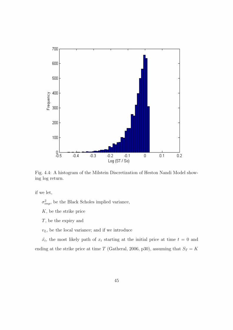
Fig. 4.4: A histogram of the Milstein Discretization of Heston Nandi Model show-ing log return.

if we let,

σ2imp, be the Black Scholes implied variance,

K, be the strike price

T , be the expiry and

vL, be the local variance; and if we introduce

xt, the most likely path of xt starting at the initial price at time t = 0 and

ending at the strike price at time T (Gatheral, 2006, p30), assuming that ST = K

45

then we have,

σ2imp ≈

1

T

ˆ T

0

vL(xt)dt. (4.20)

This is summarized very well by Gatheral:

we now have a very simple and intuitive picture for the meaning of

Black-Scholes implied variance of a European option with a given strike

and expiration: It is approximately the integral from today to expira-

tion of local variances along the most probable path for the stock price

conditional on the stock price at expiration being the strike price of

the option. (Gatheral, 2006, p31)

Applying this to the Heston model where

v, is the instantaneous variance

λ′ = λ− ρη2

where v is the mean variance of the asset,

v′ = vλλ′

this yields (4.21),

σ2imp

∣∣K=FT

≈ (v − v′)1− e−λ′T

λ′T+ v′. (4.21)

This has the consequence that

σ2imp

∣∣K=FT

→ v, T → 0

46

and

σ2imp

∣∣K=FT

→ v, T →∞

as one would expect.

It is more interesting to see how the implied volatility changes with ρ and η.

It turns out that the dependence is roughly linear. We have from (Gatheral, 2006,

p35)

δ

δxtσ2imp =

ρη

λ′T

1− 1− e−λ′T

λ′T,

(4.22)

therefore,

δ

δxtσ2imp →

ρη

2, T → 0,

and

δ

δxtσ2imp →

ρη

λ′T, T →∞.

There are straight line asymptotes which may be used for calibration. Again,

a word of warning is appropriate, options that are either very far in the money

or very far out of the money are not frequently traded, this is often the case with

very short or very long expiry options. Thus they are not a very reliable source of

information to calculate parameters, it is better to use the prices of options which

are traded in high volumes.

47

4.6 SVI Model

Based on the straight line asymptotes for σimp, Gatheral has suggested a straight-

forward model for the shape of the volatility surface. He describes this model as

Stochastic Volatility Inspired (SVI). It is based on the shape of the surface and

while it is not directly derived from the dynamics, it does work reasonably well.

We follow (Gatheral, 2006, p37) and (Gatheral, 2004). Gatheral proposes that for

k = log(K/St),

a, the overall level of variance,

b, the angle between the left and right asymptotes,

s, a measure of the smoothness of the meeting point of the asymptotes,

ρ, the orientation of the graph and

m, a translation parameter, that

σ2imp = a+ b

(ρ(k −m) +

√(k −m)2 + σ2

).

The following plot in figure 4.5 was made with a = 0.04, b = 0.4, s = 0.1, ρ =

−0.4,m = 0 and it shows the asymptotes. The equations of the asymptotes are

for the left and right

σ2imp = a− b(1− ρ)(k −m), σ2

imp = a+ b(1 + ρ)(k −m).

4.7 Estimation of the Heston Parameters

It is very difficult to estimate the parameters with a sufficiently small error. We

wish to find estimates for: v, v, λ, ρ and η, subject to the following conditions,

48

Fig. 4.5: Plot of the SVI model with implied variance against k = log(K/St) .

v ≥ 0, as it is a variance it cannot be negative,

v > 0, as a variance of a risky asset needs to be non zero,

η > 0, since the variance of the asset is stochastic,

λ > 0, as we want the volatility of the asset to revert to its mean, and

−1 < ρ < 1, as it is a correlation,

It is to be expected that the correlation ρ would actually be negative. This is

because we expect that an unexpected decrease in an asset’s value would increase

the market’s perception of its volatility, (and hence increase its actual volatility).

The basic method to estimate parameters is that for a particular option we

49

vary the five parameters so that we equate the observed market price of the option,

and the predicted value from the Heston Model. We do this simultaneously for

several combinations of strike price and expiries, and minimize the sum of the

errors. The process will hopefully yield a set of five parameters giving the least

overall error. It is common to use the sum of the squares of the errors instead of

the magnitudes of the errors. The problem with this general method is that the

minimized error, however it is calculated, in the five dimensional space might only

be a local minimum. To test all the possible combinations of five variables would

use considerable computing power, and might not be possible for each risky asset

each day. It would be considered reasonable however that once values are found

that are working well, that there would only be a daily correction rather than

an exhaustive search. For example Excel’s solver might be sufficient if nothing

serious happens between calibrations. The advantage of the Heston model for the

general problem of parameters is that we can use the explicit solution to find the

parameters starting from traded option prices. We may then use these parameters

in the Monte Carlo simulation to find the prices of exotic or path dependent

options.

This problem is discussed in (Mikhailov and Nogel, 2003), (Bakshi,Cao and

Chen, 1997) and in (Gatheral, 2006, p40).

4.8 Remarks Concerning the Heston Model

Consideration of the prices of short expiry options leads one to conclude that

the observed implied volatility level cannot be fully explained by the stochastic

volatility model of Heston. This leads to further developments of the model dealt

50

with later in this report. Rebonato suggests that the excess of implied volatility

might be a consequence of the market crash on Black Monday, 17th October 1987

(Rebonato, 2004, p439). After such a shock traders may have been prepared to

pay for a little ‘insurance’ even for a very short period of time as they consider

the possibility that the price of a risky asset might move suddenly.

51

5 Further Developments, Jump Diffusion Model

and SABR

We briefly look at two developments since the Heston Model. First the Jump

Diffusion (SVJ) model and second the Stochastic, α, β, ρ (SABR) model.

5.1 Stochastic Volatililty with Jumps (SVJ)

In the SV model risky asset prices followed a continuous process and so there was in

some sense a limit to how much an asset value could be expected to move in a small

time. Thus, an improvement to the SV model is to allow jumps. This will account

for the higher than expected short term volatility one observes, however it raises

questions about the frequency and size of these jumps. It is to be expected that

the jump diffusion will not be significantly different from the stochastic volatility

at large expiry times since the intervening time would allow the SV model to

account for the implied volatility. However the jump diffusion model will be useful

in explaining short expiry option prices.

We follow Gatheral (Gatheral, 2006, p52), who follows Wilmott (Wilmott,

2006, p931).

S is the value of the risk asset,

µ is the drift,

σ is the volatility

Z is a standard Brownian motion, which is independent of the jump process,

J is the proportion by which S changes when a jump occurs, we assume that

this is known, and

52

dq is a Poisson Process dq = 1 with probability λ(t)dt, otherwise dq = 0. Then

the SVJ model proposes that,

dS = µSdt+ σSdZ + (J − 1)Sdq

For example if J = 23, then when dq = 1, the change in S, dS is immediately

(1 − 23)S = −1

3S, that is S changes from S to 2

3S. If J = 1, there is no jump

at all. The advantage of this model is of course that it can fit the empirical data

better than the SV model as it can account for the short term implied volatility.

The disadvantage is that the mathematics is much more complicated. This is

because in addition to the needs of the SV model we must model the distribution

of the jump events and also their size. This leads to yet more parameters to be

estimated and more room for error. It would seem reasonable to look for the jump

parameters at short expiry where their effect is most pronounced, and to look at

the longer expiry data to fit the background SV model.

5.2 Stochastic α, β, ρ (SABR)

We base this discussion on Wilmott, (Wilmott, 2007, p292-293), with some input

from (Gatheral, 2006, p91-93). This model is best suited to modeling bond yields,

and other fixed income instruments which tend to have lower volatility than stocks,

currencies or commodities. It proposes that for

F the forward rate, a random quantity,

α the volatility of the forward rate, also a random quantity and,

X1, X2, two standard Brownian motions with correlation ρ

53

that

dF = αF βdX1,

and

dα = vαdX2.

There are three parameters, namely, α, β, ρ. The advantage of this method is that

there are good closed form approximations for the cases where the volatility α and

the volitility of the volatility v are both low. This is the case for bonds. Another

advantage is that there are only three parameters to be estimated instead of the

five of the Heston model.

54

6 Conclusion

1n 1973 the Black Scholes Merton model was published. This made a huge differ-

ence to the pricing of options all over the financial world. As with any model it

has to make assumptions about the market, these are (Gemmill, 1997, p14):

• the asset price is lognormally distributed, i.e. the returns on the asset are

normally distributed,

• the distribution of the returns is constant,

• there are no transaction costs, so that hedging may be done without fees,

• the risk free interest rate is constant, and

• there are no dividends.

Quoting from Rebonato,

Once we recognize that the assumptions of the Black-and-Scholes world

are so strongly violated that we have to introduce a strike dependence

on the implied volatility, the latter quantity simply becomes the wrong

number to put in the wrong formula to get the right price of plain-

vanilla options ’ (Rebonato, 2004, p169, italics his).

It is clear that the CV model needs to be improved. The Heston model relaxes the

first and second assumptions. We have shown in the Monte Carlo simulations that

SV is more realistic than constant volatility models, we have also proposed that

SV is not the end of the story and that the SVJ models might be an improvement.

This is clearly a good direction for further study.

55

There are wider questions one can raise in this field. As one builds models of

market behaviour what units of time should be used? Is it reasonable to assume

that chronological time is sufficient? What about gaps between trading days, do we

ignore these gaps? Would it be better to use the sequence of trades or the number

of shares sold, as units of time? Can we assume that all trades are actually done

for the purpose of trading or can there be other reasons, for example tax benefits?

There are more questions in this field than one can hope to address.

Consider the path of a projectile near the surface of the earth. A first model of

its trajectory is to ignore air resistance and assume gravity is constant and parallel,

this gives us the familiar parabolic path. By the time we incorporate air resistance

and the rotation of the earth we have some very messy mathematical equations

but we have a more accurate model. This is the level we may be at with with the

improvement from CV to SV, SVJ and SABR models. We are certainly nowhere

near the hermeneutic change from Newtonian physics to relativistic mechanics with

it’s extreme accuracy. It might however be permissible to quote from Einstein,

As far as the laws of mathematics refer to reality, they are not certain;

and as far as they are certain, they do not refer to reality.’(J R Newman,

1956)

It is unlikely that economic phenomena will ever be as predictable as physical

phenomena, not while trading decisions are made by human beings and their

computer programmes. So, we are left chasing the gold at the end of the rainbow...,

and occasionally finding some.

56

This section of the report contains the code used in the computer programmes

which did the calculations producing the tables and graphs.

A Numerical Integration

A.1 Matlab Code for Explicit Solution

The following Matlab code, D.m and F.m, was used to evaluate the functions D

(4.16) and F (4.19).

function [DJ]=D(u,j)

% We begin by entering the Heston parameters used here

lambda = 1.3253; rho =-0.7165; eta = 0.3877;

% This is a constant which we may vary at some stage

tau = 1/250;

% These are the intermediary functions

alpha = -u2/2 -1i*u/2 + 1i*u*j; beta = lambda-rho*eta*j

- rho*eta*1i*u; gg = eta2/2; d = sqrt(beta2 - 4*alpha*gg);

rm = (beta - d)/eta2; rp = (beta + d)/eta2; g = rm/rp;

% We define D

DJ=rm*(1-exp(-d*tau))/(1-g*exp(-d*tau));

57

function [FJ]=F(u,j)

% We begin by entering the Heston parameters used here

lambda = 1.3253; rho =-0.7165; eta = 0.3877;

% This is a constant which we may vary at some stage

tau = 1/250;

% These are the intermediary functions

alpha = -u2/2 -1i*u/2 + 1i*u*j; beta = lambda-rho*eta*j

- rho*eta*1i*u; gg = eta2/2; d = sqrt(beta2 - 4*alpha*gg);

rm = (beta - d)/eta2; rp = (beta + d)/eta2; g = rm/rp;

% We define F

FJ=lambda*( rm*tau - (2/eta2)*log((1-g*exp(-d*tau))/(1-g))

);

Using the above code to calculate F and D, the integrals P1 and P0 of (4.18)

were calculated using the following code, P.m.

function [PJ] = P(j,x)

% We enter the remaining Heston parameters

58

vbar =0.0354; v =0.0174;

% We evaluate the integral in 2.13 of p19 of Gatheral, 2006

gap = 0.001; PJI=0;

for z=1:fix(1000/gap) PJI=PJI+ real((exp(F(z*gap,j)*vbar + D(z/1000,j)*v

+ 1i*(z*gap)*x))/(1i*(z*gap))); end PJ= 1/2 + (1/pi)*PJI*(gap);

Finally the price of a call option was calculated using C.m. To operate this

just enter the stike price, K.

function [CJ]=C(K)

% From eqn 2.5 on p17, Gatheral, 2006

x=log(1227.73/K); CJ=1227.73*P(1,x)-K*P(0,x);

A.2 Programmes Supporting Reliability of the Explicit So-

lution

Q.m is the integrand of (4.18) which is taken from zero to infinity. The aim of

this is to show that 1,000 is large enough to give a reliable upper limit for the

numerical integral.

59

function [PJI] = Q(j,x,u)

% We enter the remaining Heston parameters for 15th Sept 2005

vbar =0.0354; v =0.0174;

PJI = real((exp(F(u,j)*vbar + D(u,j)*v + 1i*(u)*x))/(1i*(u)));

PlotofM.m shows that it is reasonable to calculate (4.18) with an upper limit

of 1,000.

function[K] = PlotofM(K)

x=log(1227.73/K); M=0;N=0; % R is the resolution of the plot, i.e. the number of points used

R=50; for b=1:R N(b)=b*10; M(b)=K*(exp(x)*Q(1,x,10*b)-Q(0,x,10*b));

end plot(N,M) StrikePrice = K;

B Monte Carlo Milstein Discretization

Table 4.2 was obtained using the following Matlab code on an Intel dual core

using Matlab Version 7.2.0232 (R2006a). The second version referred to in the

text was made using an Intel Celeron 1.6GHz, Matlab Version 7.7.0 (R2008b) and

60

used more iterations, N = 20, 000 instead of N = 5, 000, and a smaller time gap,

∆t = 10−6 instead of ∆t = 10−5. It produced almost the same results, but took

about six time as long to run.

Milstein.m is the Matlab programme which used the Monte Carlo method to

calculate asset prices and hence option prices using the Milstein Discretization

from Gatheral, 2006, p22.

% The results from this one seem quite reasonable. using N=5000 and

% dt=0.00001.

% We use the initial price ’So’ note use of lower case letter as it

% looks better.

% We get the final price and the price of a plain vanilla.

% Milstein Discretization of the Heston Model page 22 of Gatheral with

% parameters from p40, ie the 15th of Sept 2005.

function [K]= Milstein(K,eta,lambda,vbar,dt,T,So,rho,v0)

if nargin < 1 K = 1160 ; end; if nargin < 2 eta = 0.3877; end; if

nargin < 3 lambda = 1.3253; end; if nargin < 4 vbar = 0.0354; end;

if nargin < 5 dt = 10-6; end; if nargin < 6 T = 1/250; end; if nargin

< 7 So = 1227.73; end; if nargin < 8 rho = -0.7165; end; if nargin

< 9 v0 = 0.0174;

61

end; % x = log( S_t / So ), it’s not the stock price, so it can be negative

for N=1:5000

x0 = 0; v = v0; x = x0; xx=0; vv=0; SToverSo = 0;

for j=1:(floor(T/dt)); R1 = randn; R2 = randn; v = abs((sqrt(v) +

(eta/2) * sqrt(dt) * R1)2 - lambda * ( v - vbar) * dt - (eta2)/4

* dt); x = x + sqrt(v * dt) * ( rho *R1 + sqrt(1-rho2) *

R2 ); % xi = log of Si/So. We have used the formula for a bivariate

% normal distribution from Glasserman, 2004, p72.

vv(j) = v; xx(j) = x;

end

% Here we calculate ST/So

SToverSo(N) = K*exp(x); Result(N) = x; %this is a plot like fig 4.1 on p.45 of Gatheral

%Here we calculate the price of plain vanillas

62

Call(N) = max(So*exp(x) - K,0); Put(N) = max(K - So*exp(x),0);

end

% We may display the output with the command

hist(Result,40);

MeanEndpriceST = mean(SToverSo);

% Calculating the price of the options and 95% confidence intervals

MeanofCall = mean(Call) ConIntCall = 1.96*std(Call)/sqrt(N)

MeanofPut = mean(Put) ConIntPut = 1.96*std(Put)/sqrt(N)

63

References

[1] Bakshi,G., Cao, C. and Chen, Z.:Empirical Performance of Altermative Op-

tion Pricing Models, The Journal of Finance 52, 2003-2049, 1997.

[2] Cont R., Tankov P.:Financial Modelling With Jump Processes, Florida: Chap-

mam & Hall, 2004.

[3] Derman E. and Kani I.:RISK Volume 7., No 2 February (1994).

[4] Derman E. and Kani I.:Stochastic implied trees, Arbitrage pricing with

stochastic term and strike structure of volatility. International Journal of

Theoretical and Applied Finance Vol 1, 61 - 110: 1998.

[5] Dettman, J.W.:Applied Complex Variables, New York: Dover, 1984.

[6] Duffie D., Pan J., and Singleton K.: Transform analysis and asset pricing for

affine jump diffusions, Econometrica 68, 1343 - 1376, (2000).

[7] Gatheral, J.:A parsimonious arbitrage-free implied volatility parametrization

with application to the valuation of volatility derivatives, a paper presented

at Global Derivatives and Risk Management in Madrid on 26th May 2004.

[8] Gatheral, J.:The Volatility Surface A Practitioner’s Guide, New Jersey: Wiley

2006.

[9] Gemmill, G.:Black-Scholes, in: D. Paxso (ed.) and D. Wood (ed.) The Black-

well Encyclopedic Dictionary of Finance, Oxford: Blackwell Business 1977.

[10] Glasserman, P.:Monte Carlo Methods in Financial Engineering, Springer,

2004.

64

[11] Heston, S.:A closed-form solution for options with stochastic volatility, with

application to bond and currency options, Review of Financial Studies 6,327

- 343, 1993.

[12] Kahl, C. and Jackel P.:Not so complex logarithms in the Heston Model,

Wilmott Magazine,Wiley, 94-103, 2005.

[13] Mikhailov S. and Nogel U., Heston’s Stochastic Volatility Model Implemen-

tation, Calibration and Some Extensions, Wilmott Magazine, Wiley, 74 - 79,

2003.

[14] Newman, J.R.:The World of Mathematics : New York 1956.

[15] Rebonato, R.:Volatility and Correlation the Perfect Hedger and the Fox, 2nd

edition Chichester: Wiley, 2004.

[16] Taleb, N.:The Black Swan - The Impact of the Highly Improbable, London:

Penguin, 2007.

[17] Wilmott, P.:Paul Wilmott on Quantitative Finance (Volume 3.), Chichester:

Wiley, 2006.

[18] Wilmott, P.:Frequently Asked Questions in Quantitative Finance, Chichester:

Wiley, 2007.

65