0 HETERODOX PRODUCTION AND COST THEORY OF THE BUSINESS ENTERPRISE By Professor Frederic S. Lee The 4 th Bi-Annual Cross-Border Post Keynesian Conference 9-10 October 2009 Professor Frederic S. Lee Department of Economics University of Missouri-Kansas City 5100 Rockhill Road Kansas City, Missouri 64110 USA E-mail: [email protected]
Transcript
0
HETERODOX PRODUCTION AND COST THEORY OF THE
BUSINESS ENTERPRISE
By
Professor Frederic S. Lee
The 4th Bi-Annual Cross-Border Post Keynesian Conference 9-10 October 2009
Professor Frederic S. Lee Department of Economics
University of Missouri-Kansas City 5100 Rockhill Road
Heterodox economists complain about having no systematic alternative to neoclassical
production and cost theory. The complaint seems somewhat inaccurate since over the last seventy
years alternatives have been broached, starting with Gardiner Means, Philip Andrews, Joel Dean and
Piero Sraffa and more recently Alfred Eichner (Lee, 1986, 1998). However, there is also a
reasonable germ of truth to it as long as the alternative theory had to contain or mirror all of what
constitutes neoclassical production and cost theory. What the heterodox alternatives failed to do was
to adequately delimit themselves from their neoclassical brethren and to clearly articulate what an
alternative production and cost theory would covered and what it would not. For example, most
heterodox alternatives dismissed marginal products, but they did not extend their arguments to cost
minimization, to marginal cost curves, or to constant output factor input demand curves. Moreover,
most of the alternatives dealt with short period production and costs, but left open the possibilities
for long period production and costs based on, implicitly, neoclassical returns to scale arguments. If
any real progress is to be made in developing a heterodox theory of production and costs, it must be
accompanied with empirically-based arguments that establishes its theoretical domain and at the
same time rejecting the domain of neoclassical theory on the grounds that it is empirically
ungrounded and theoretically irrelevant. What follows is a preliminary attempt to do precisely this:
to develop a heterodox theory of production and costs of the business enterprise and delineate its
domain relative to the domain of neoclassical production and cost theory.
The business enterprise produces an array of outputs, that is, goods and services or product
lines. A product line may consist of a single main product with numerous derivative but secondary
2
and/or by-products; or it may consist of a conceptually distinct product that is a differentiated array
of products. In either case, the structure of production of a single product in a product line is hard to
isolate because fixed investment goods and labor power skills may be used to produce more than one
product; and the costing of the product is difficult because of the problem of allocating various
common shop costs. To overcome this, the product line is defined in terms of its core or main
product—that is, a product line consists of a single homogeneous product. As a going concern, when
producing any product line, the business enterprise engages in sequential acts of production through
historical time and as a result incurs sequential costs of production also through time. These acts of
production and the costs incurred in producing a product line are determined by the underlying
relatively enduring structures of production and costs. The structure of production consists of plant
segments-plant, shop technique of production, and the enterprise technique of production; and
correspondingly, the cost structure of the product line consist of direct costs, shop expenses and
enterprise expenses (jointly called non-direct costs). The basic analysis of the structure of
production and costs is a two dimensional comparative analysis in which production and costs are
examined relative to different flow rates of output (or degrees of capacity utilization). Hence it
concentrates on the "virtual" movement of inputs and costs and the flow rate of output. From this it
is possible to delineate a time-oriented structure of production and costs with regard to sequential
and different variations in the flow rate of output, but it will not be covered in this paper.
Before delving into the theory of production and costs, it is first necessary to delineate and
discuss the accounting rules by which enterprises identify, understand, and record their costs. Once
this is in place, the ensuing sections deal with the structures of production and costs as they relate to
plant segments, plants, and direct costs; the structures of production and costs regarding the shop and
enterprise techniques of production and shop and enterprise costs; and the structure of production
3
and average total costs for the product line. The final section of the paper summarizes the theory by
comparing it to and differentiating from and compares it to neoclassical production and cost theory.
Accounting Rules
The business enterprise adopts and develops cost and financial or, more generally, managerial
accounting practices that are necessary for it to be a going concern. So long as the enterprise
remains a going concern, its accounting practices remain relatively enduring, although changing in
minor ways in light of changes in technology, inputs used in production, and the information needs
of management. If an enterprise is not a going concern, it is a terminal venture in that it has a
specific starting and ending date. Consequently, accounting for expenditures as deductions or one-
time expenses against revenue, revenue, and business income is straightforward. Moreover, the
question of the value of the fixed investment goods and depreciation never arises. That is, the fixed
investment goods are valued at the beginning of the venture and then revalued at the terminal date.
Their initial value is their historical costs while their liquidation value at the terminal date is added to
the profit account for distribution (Litherland 1951). An enterprise as a strictly terminal venture is
largely incommensurate with a going concern economy; rather it is compatible with an exchange
economy where repeatable and ongoing economic activities and provisioning process are absent. As
for the going enterprise, the accounting practices must ensure an accurate delineation of costs which
must be recovered if the enterprise is to be a going concern. More specifically, because a going
enterprise engages in continuous sequential acts of production, its income or profits has to be
calculated periodically, which is denoted as the accounting period and is generally taken to be a
calendar year, and in a manner that permits distributing part of it as dividends without impairing the
enterprise’s productive capabilities. This means it is necessary to treat inputs (which are producible
and reproducible) that contribute to the production of the output as reoccurring costs as oppose to
4
one-time expenses against total revenue to arrive at profits.1 In this manner, the expenses of
resources, goods, services, labor power skills, depreciation of fixed investment goods used directly
and/or indirectly in production are costs that are recouped so that the enterprise can repeat
production. This implies that the fixed investment goods are not viewed as commodities to be sold
on the market for revenue purposes; rather the going enterprise views them as essential non-
commodities for maintaining the going plant whose historical value is considered a recoverable cost
to be changed against revenue before determining business income.
The accounting practices essential to a going concern deal with (1) the tracing of the direct
and overhead material, services, resources, and labor skills inputs relevant to the production of a unit
of output, (2) the categorization of costs into direct (variable) and overhead (fixed) costs, (3) the
determination of the cost of producing a unit of output, (4) depreciation, and (5) the determination of
profits associated with a particular product and the business income for the enterprise as a whole.
Evidence from archives of business enterprises show that prior to 1700 merchants utilized
accounting systems to keep records of purchases and sales; and after that, industrial enterprises drew
on these systems to keep records of purchases and sales, and to document the internal movement of
inputs in the production process. In particular, sophisticated cost accounting systems for tracking
direct inputs and direct costs in the production of a specific good have been in use since the 1700s.
At almost the same time, enterprises developed accounting procedures that differentiated between
1 That is, costs are defined in terms of the going enterprise, so that what constitutes costs are reoccurring expenses derived from the use of reproducible intermediate inputs, labor power skills, and fixed investment goods. Such costs are objective and irreducible to a homogeneous unit such as labor or subjective disutility. Moreover, non-produced items that are not utilized on a reoccurring basis are not costs but expenses that are charged against revenue. Therefore, scarce factor inputs are not costs in the context of the going enterprise, which means that the category of costs of the going enterprises is conceptually distinct from the category of costs in neoclassical theory in that the former is not based on relative scarcity. [Kurz and Salvadori, 2005]
5
direct and overhead inputs and costs, began identifying and measuring/quantifying them, and devised
procedures to allocate the overhead costs among the various goods produced.2 Thus by 1900
comprehensive accounting systems of various degrees of sophistication were in general use and
remain so to the present day. With developed cost accounting systems in hand, enterprises are able
to engage in costing of a good, that is, to arrive at its unit (or average) direct or direct plus overhead
cost.3 Costing systems utilized historical-estimated, or standard costs and employed various methods
(based on, for example, output, direct costs, direct labor costs, labor hours, or machine hours) for the
allocation of overheads.4 However, changes in technology, the production of new goods and
services, the need for new and better product line cost information, and competitive pressures have
pushed enterprises to alter their cost accounting and costing systems although not significantly, but
their function of collecting cost information and use for estimating product line costs has remained
unchanged—as long as enterprises remain going concerns, cost accounting and costing systems will
2 The term ‘direct’ input/cost refers to inputs and costs that are directly associated with the production of a good; while ‘overhead’ input/cost refers to an input/cost that is not directly associated with the production of a good. Direct and overhead are not the same as variable and fixed; and accountants and business enterprises generally did not use those concepts until the latter part of the twentieth century, when the accounting profession began acquiring the concept from economics. While not identical, they are in practice pretty much the same and for theoretical purposes with regard to pricing and the determination of profits, the differences are not important. Thus for this paper, direct and overhead will be used. 3 The costing of unit direct costs (or what is called ‘direct’ or ‘marginal’ costing) is done only under special circumstances, if the accounting procedures employed do not permit more detailed costing to take place, or if management is not interested in a better understanding of its costs. But in general, enterprises undertake total (absorption) costing which includes both direct and overhead costs. 4 There are two types of costing procedures, historical-estimated and standard costing. In the former, costs are determined by methods that range from a perfunctory guess to a very careful computation based upon past experience; in either case, past costs are used as the basis to determine the costs of a good that will be produced in the future. In the latter, costs are determined in advance of production by a process of scientific fact-finding that utilizes both past experience and controlled experiments. However, in spite of the differences, both historical-estimated and standard costing arrive at the costs of producing a good that will be used in setting the price in the same way.
Jones 1985; Boyns and Edwards 1995; Boyns, Edwards, and Nikitin 1997; Fleischman and Parker
1997; Lee 1998: Appendix A; Al-Omiri and Drury, 2007]
Business enterprises have always made financial decisions, such setting prices, whether to
produce a good or close down a product line, or undertake an investment project; and tying costing
systems to the financial decisions (which occurred as early as 1700) helped immensely in making the
decisions. This long historical emergence was, in part, due to an interlinked problem qua
controversy grounded in the nature of a going concern. In particular, profits are defined as the
difference between revenue and costs for a particular period of time, such as the accounting period,
but whether that definition is consistent with the nature of the going concern depends on how
expenditures on fixed investment goods are accounted for. From 1700 into the early 1900s,
expenditures on fixed investment goods paid for and expensed out of revenues or profits and not
included as a cost component, that is depreciation, of a product. Being treated as a current expense
and hence not added to the capital account, the capitalized value of the enterprise did not change.
More significantly, it also meant that the enterprise’s cost structure did not include all the costs to be
a going concern—that is, it did not include the cost of the fixed investment goods needed for ongoing
and future production. So when the fixed investment goods wore out or became technologically
obsolete and thus needed to be replaced, a ‘cost-recovery’ fund for their replacement purchase did
not exist.
Enterprises dealt with the problem through adopting replacement accounting in which
5 In recent decades various studies have noted the relative stability in accounting practices used by enterprises. They show that enterprises slowly make marginal changes while retaining basic practices, even when faced with a changing environment. [Emore and Ness 1991; Bright et. al 1992; Granlund, 2001]
7
replacement (which could include repairs) investment was charged directly against revenues before
profits were determined; having repairs to the fixed investment goods (which is a form of
investment) charged directly against revenues before profits were determined; or establishing a
depreciation fund of money based on assigned depreciation rates (based on reducing balance, straight
line, or some other basis) to different categories of fixed investment goods based on their historical
costs, which involved a charge against revenue before profits were determined or directly against
profits.6 However, the demand by shareholders of the enterprise for immediate dividends
irrespective of the negative impact on the going concern capabilities of the enterprise to provide an
ongoing stream of dividends and hence an ongoing access to the provisioning process resulted in a
change in the way expenditures on fixed investment goods were dealt with.7 Instead of being
expenses charged against revenue, they initially are expenditures out of profits that become a cost of
production.8 To include depreciation as a cost of production, it is first necessary to value the fixed
investment goods, which is generally done at historical cost (that is in terms of money). Then a
method of depreciation, such as straight-line or accelerated, is deployed to determine the amount of
depreciation to be allowed as a cost of production. Once depreciation is a cost of production, the
accounting working rules of the enterprise ensure that, in principle, all inputs are traceable, all costs
identified and allocated, and the determination of business income or profits can be done without
6 Allocations to the depreciation fund often varied directly with profitable years (Stone 1973-74; Edwards 1980). 7 There was another controversy which involved whether ‘interest’ on the paid in ‘capitalized value’ of the enterprise was a cost or not. In some partnerships, interest charges were included as costs in order “to ensure that individuals were properly remunerated for differential capital contributions rather than to produce a more accurate costing of business operations’ (Edwards 1989: 312; also see Stone 1973-74; Hudson 1977). While this case seems to be the basis of mainstream arguments that includes normal profits as costs, generally interest charges are not considered costs. 8 This means that fixed investment goods are not seen as commodities to be sold to raise revenue, but as a cost of production to be recovered.
8
affecting the going plant of the enterprise.9 [Edwards 1980, 1986, 1989; Boyns and Edwards 1997;
Napier 1990; Tyson 1992; Fleischman and Parker 1997; Wale 1990]
Technology, Plants, and Direct Costs
The basic aggregate unit of production is an establishment which houses or encompasses the
activities immediately involved in the production of the product line—it is denoted as the plant.
Given the plant, production can be further delineated in that more than one plant may be used to
produce the product line and/or that each plant may consist of a number of plant segments, each also
capable of producing the product line. Whether the plant is an emergent technological establishment,
divided into separate plant segments, or a hybrid of the two depends on the technology constituting
the plant.10 Although the production of a product line may consist of many processes and stages, the
enterprise’s cost accounting procedures are capable of tracking each direct intermediate and labor
power input and their amount used in production. Consequently, the array of direct inputs used in
production of a unit of output constitutes and represents the technology used in production.
Plant Segment, Plant, and the Structure of Production
For the segmented plant (SP), the primary unit of production is the plant segment (PS) which
is defined as the technical specifications of direct intermediate inputs of resources, goods, and
services and labor power skills needed to produce a given amount of output, g, of a product line in a
specific period of time. This usage of direct inputs, is, in turn, uniquely determined by the
specifications of the plant segment and underlying fixed investment goods (K = k1,…, kk), and the
9 The old method of expensing the purchases of fixed investment goods meant that the capitalized value of the enterprise did not alter. Consequently, the concept of the rate of profit under this system had no precise meaning, making it useless as a theoretical concept. Although the introduction of depreciation partially redresses this issue, the use of historical cost makes the rate of profit a backward looking concept, hence ill-suited as a theoretical tool. 10 For evidence of the three types of plants, see Lee (1986).
9
social/labor conditions surrounding production. Moreover, the fixed investment goods used in
production of g are uniquely related to it in that they are is specifically tailored to produce g per
period of calendar time. The period of time used in the specification of the PS is called the
production period and it denotes the amount of calendar time needed to produce g, starting with the
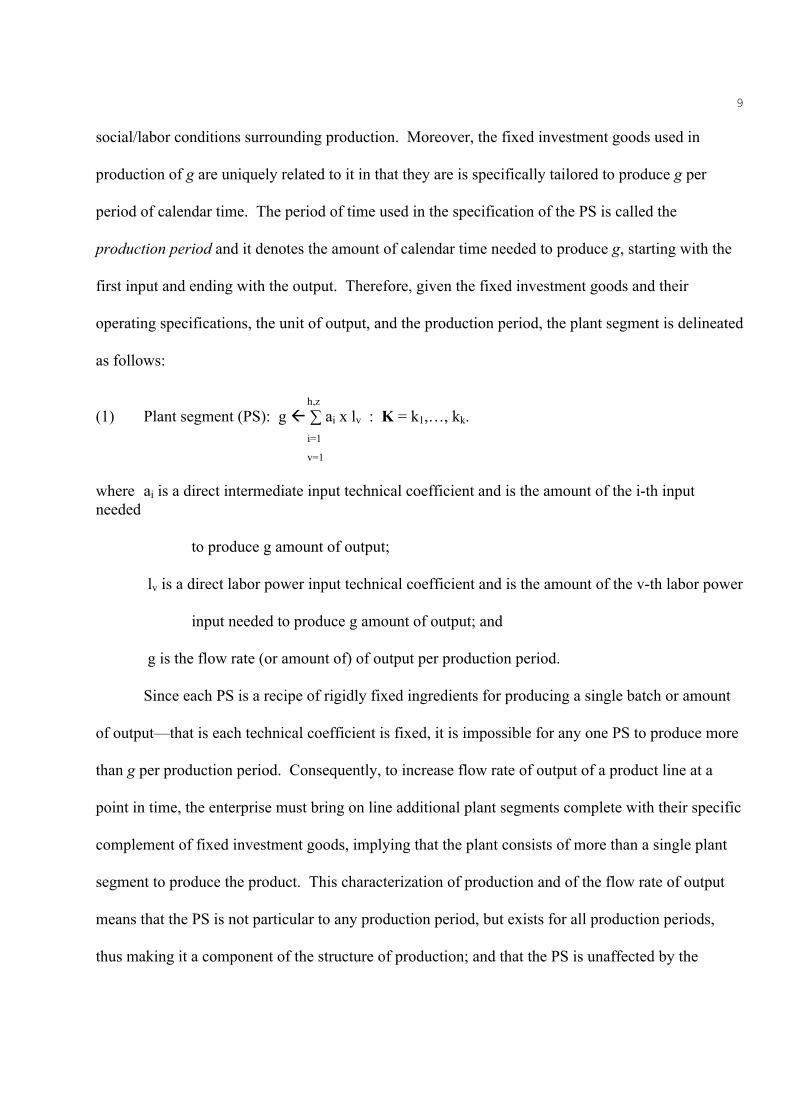
first input and ending with the output. Therefore, given the fixed investment goods and their
operating specifications, the unit of output, and the production period, the plant segment is delineated
as follows:
h,z (1) Plant segment (PS): g ∑ ai x lv : K = k1,…, kk. i=1 v=1 where ai is a direct intermediate input technical coefficient and is the amount of the i-th input needed to produce g amount of output; lv is a direct labor power input technical coefficient and is the amount of the v-th labor power input needed to produce g amount of output; and g is the flow rate (or amount of) of output per production period.
Since each PS is a recipe of rigidly fixed ingredients for producing a single batch or amount
of output—that is each technical coefficient is fixed, it is impossible for any one PS to produce more
than g per production period. Consequently, to increase flow rate of output of a product line at a
point in time, the enterprise must bring on line additional plant segments complete with their specific
complement of fixed investment goods, implying that the plant consists of more than a single plant
segment to produce the product. This characterization of production and of the flow rate of output
means that the PS is not particular to any production period, but exists for all production periods,
thus making it a component of the structure of production; and that the PS is unaffected by the
10
passage of time or by repeated usage through time even though it must exist in time. As a result, this
relatively enduring structural property permits the PS to be used over and over again under the guise
of sequential production. In this manner, the fixed technical coefficients are flow coefficients and g
is a flow of output denominated in terms of a single production period.11
Consider the case for the segmented plant when the plant segments of a plant are not
identical, meaning that each PS consists of different amounts of the same inputs or of different
inputs.12 If m plant segments are being used, where 1 < m < maximum number of plant segments in
the plant, then we have
m m h,z (2) Segmented plant: qm = ∑gj ∑ ∑ aij x lvj : Ksp = k1m,…, kkm. j=1
j=1 i=1
v=1 where qm is the plant’s aggregate flow rate of output for m plant segments; kkm is the quantity of the k-th fixed investment good associated with the m plant segments that constitute the segmented plant; and Ksp is the vector of fixed investment goods associated with the segmented plant. From equation (2), the average amount of direct intermediate and labor power inputs used to produce
a unit of output at a given flow rate of output is derived by dividing by qm:
h,z
11It also can be noted that the characterization of the PS sweeps away the property of single (or multiple) input-output variation—that is the marginal products for intermediate and labor power inputs do not exist. Since an increased flow rate of output requires additional plant segments complete with their specific complement of K fixed investment goods, it is impossible to argue that an increase in the flow rate of output can occur by simply increasing one, some, or all the direct intermediate and labor inputs. Consequently, not only are marginal products, the law of variable proportions, and ‘convexity’ inapplicable to this analysis, but the traditional distinction between fixed and variable inputs is also undermine. 12It is possible that technically different plant segments can produce different flow rates of output, but this will be ignored.
11
(3) average plant segment (APS): 1 = qm ∑ a*i x l*
v : Kmu qm i=1 v=1 m where a*
i = ∑ aij/qm is the i-th average plant intermediate production coefficient at qm; j=1 m l*
v = ∑ lvj/qm is the v-th average plant labor power production coefficient at qm; and j=1 Kmu = qm/qmax represents the degree of capacity utilization of the plant where qmax is the plant’s maximum flow rate of output when all plant segments at utilized. The average plant segment and its production coefficients (which are input-output ratios) represent
the plant’s structure of production at different flow rates of output or capacity utilization. If the plant
segments are different, then production coefficients will vary, as will the APS, as capacity utilization
increases. However, if the plant segments of the plant are all identical, the outcome of an increase in
the flow rate of output or Kmu is
m m h,z (4) qm = ∑gj ∑ ∑ aij x lvj : Ksp j=1 j=1 i=1
v=1 h,z h,z or qm qm ∑ (ai x lv) = ∑ (aiqm x lvqm) : Ksp. i=1 i=1 v=1 v=1 since qm = mg = m. From equations (3) and (4), the average plant segment of the segmented plant is:
h,z h,z (5) APS: 1 qm ∑ (ai x lv) = ∑ (a*
i x l*v) : Kmu
qm i=1 i=1 v=1 v=1 since aiqm/qm = a*
i = ai; and lvqm/qm = l*
v = lv.
12
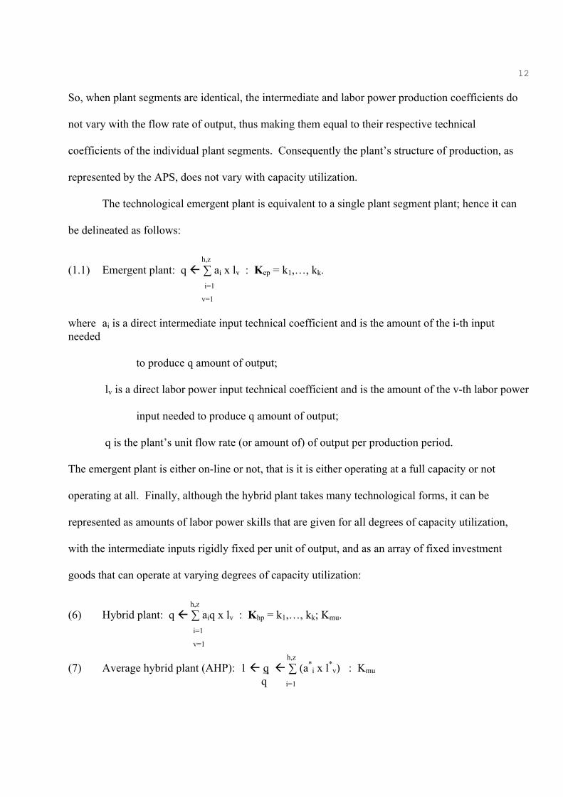
So, when plant segments are identical, the intermediate and labor power production coefficients do
not vary with the flow rate of output, thus making them equal to their respective technical
coefficients of the individual plant segments. Consequently the plant’s structure of production, as
represented by the APS, does not vary with capacity utilization.
The technological emergent plant is equivalent to a single plant segment plant; hence it can
be delineated as follows:
h,z (1.1) Emergent plant: q ∑ ai x lv : Kep = k1,…, kk. i=1 v=1 where ai is a direct intermediate input technical coefficient and is the amount of the i-th input needed
to produce q amount of output; lv is a direct labor power input technical coefficient and is the amount of the v-th labor power input needed to produce q amount of output; q is the plant’s unit flow rate (or amount of) of output per production period.
The emergent plant is either on-line or not, that is it is either operating at a full capacity or not
operating at all. Finally, although the hybrid plant takes many technological forms, it can be
represented as amounts of labor power skills that are given for all degrees of capacity utilization,
with the intermediate inputs rigidly fixed per unit of output, and as an array of fixed investment
goods that can operate at varying degrees of capacity utilization:
v = lv/q. So, when Kmu increases to the technically specified full capacity utilization of all fixed investment
goods, the intermediate production coefficient remains constant while the labor power production
coefficient declines, which means the hybrid plant’ structure of production also varies.
To summarize, the basic aggregate unit of production is the plant. Whether it is a segmented,
emergent, or hybrid plant, production is a recipe of fixed ingredients that results in fixed technical
coefficients. Hence, the intermediate and labor power inputs are not individually productive; instead
to be productive all inputs must be used together along with the associated fixed investment goods.
When the capacity utilization of the plant increases, the resulting production coefficients may
increase, decrease, or remain constant, even though the underlying technical coefficients are fixed;
and the changes are a result of the technology embodied in the plant, not the outcome of some law of
production. So how a plant’s structure of production, as represented by APS and AHP, varies with
changes in Kmu can only be determined by empirical investigations, not by assumption. [Lee, 1986;
Dean, 1976; Eichner, 1976]
Plant Segment, Plant, and the Structure of Average Direct Costs
With the introduction of intermediate input prices and wage rates, the plant segment becomes
the direct costs of the product line produced by the plant
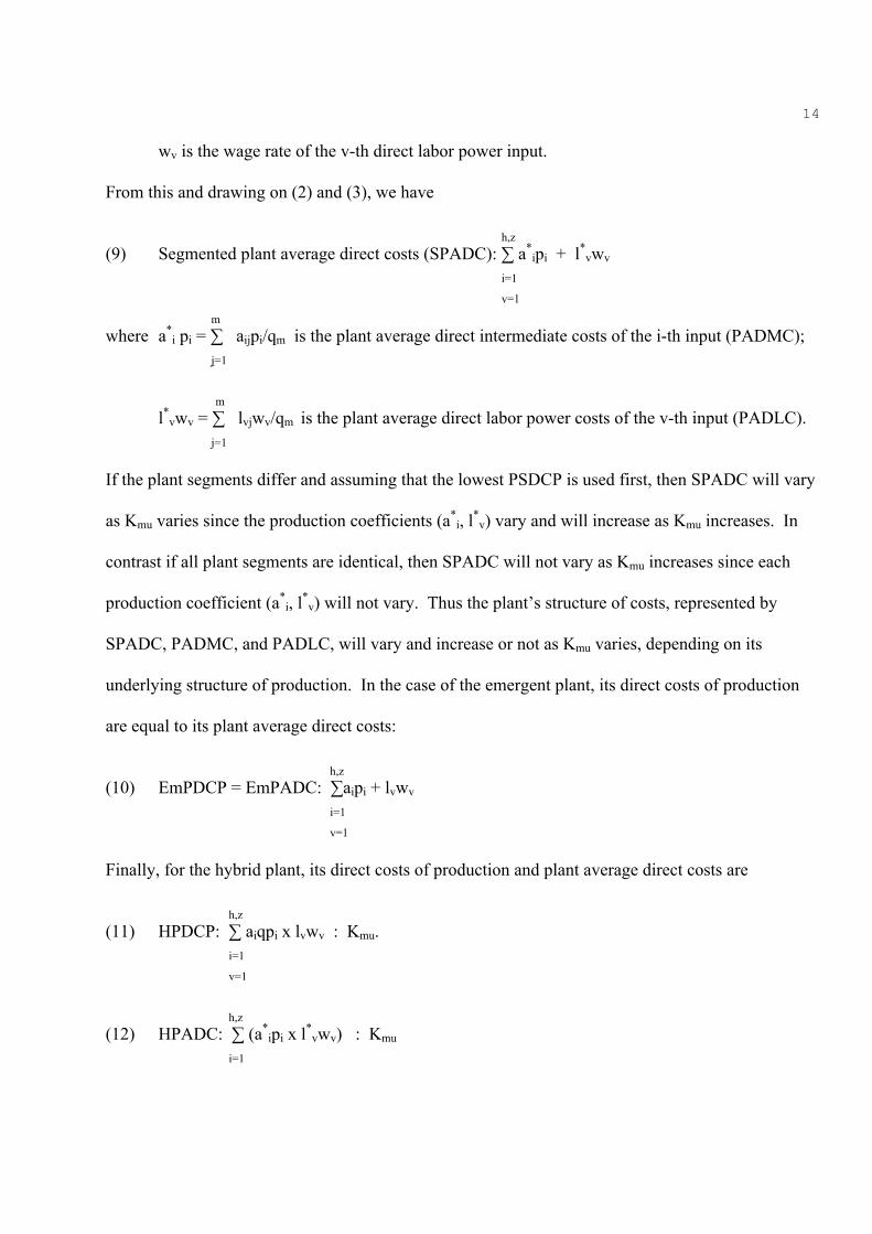
h,z (8) Plant segment direct cost of production (PSDCP): ∑aipi + lvwv i=1 v=1 where pi is the price of the i-th direct intermediate input; and
14
wv is the wage rate of the v-th direct labor power input. From this and drawing on (2) and (3), we have
h,z (9) Segmented plant average direct costs (SPADC): ∑ a*
ipi + l*vwv
i=1 v=1 m where a*
i pi = ∑ aijpi/qm is the plant average direct intermediate costs of the i-th input (PADMC); j=1 m l*
vwv = ∑ lvjwv/qm is the plant average direct labor power costs of the v-th input (PADLC). j=1 If the plant segments differ and assuming that the lowest PSDCP is used first, then SPADC will vary
as Kmu varies since the production coefficients (a*i, l*
v) vary and will increase as Kmu increases. In
contrast if all plant segments are identical, then SPADC will not vary as Kmu increases since each
production coefficient (a*i, l*
v) will not vary. Thus the plant’s structure of costs, represented by
SPADC, PADMC, and PADLC, will vary and increase or not as Kmu varies, depending on its
underlying structure of production. In the case of the emergent plant, its direct costs of production
are equal to its plant average direct costs:
h,z (10) EmPDCP = EmPADC: ∑aipi + lvwv i=1 v=1 Finally, for the hybrid plant, its direct costs of production and plant average direct costs are
ipi = aiqpi/q is the plant average direct intermediate costs of the ith input; and l*
vwv = lvwv/q is the plant average direct labor power costs of the vth input. So as Kmu increases PADMC is constant since the intermediate production coefficient is constant,
while PADLC declines as Kmu increases because the labor power production coefficient declines;
thus as Kmu increases up to full capacity utilization, PADC declines because of its underlying
structure of production. To summarize, the plant’s structure of average direct costs, as represented
by SPADC, HPADC, PADMC, and PADLC, can vary in any direction with changes in Kmu
depending on its underlying structure of production. [Lee, 1986]
Multi-Plant Production and Enterprise Average Direct Costs of Production
Business enterprises may employ up to p plants to produce a product line. Thus the number
of plants actually used in production depends on the total flow rate of output as well as the flow rate
of output of each plant. Consequently the shape of the enterprise's average direct costs curve
depends on which plants are being utilized and the degree of utilization of each plant. Focusing on
the k-th plant and assuming full capacity utilization, we have
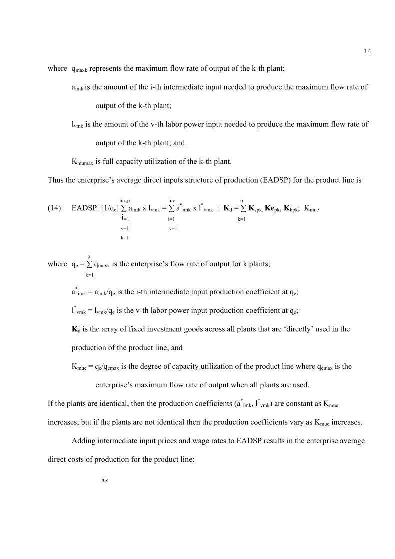
where qmaxk represents the maximum flow rate of output of the k-th plant; aimk is the amount of the i-th intermediate input needed to produce the maximum flow rate of output of the k-th plant; lvmk is the amount of the v-th labor power input needed to produce the maximum flow rate of output of the k-th plant; and Kmumax is full capacity utilization of the k-th plant. Thus the enterprise’s average direct inputs structure of production (EADSP) for the product line is
h,z,p h,v p (14) EADSP: [1/qe] ∑ aimk x lvmk = ∑ a*
imk x l*vmk : Kd = ∑ Kspk, Kepk, Khpk; Kmue
i=1 i=1 k=1
v=1 v=1
k=1
p where qe = ∑ qmaxk is the enterprise’s flow rate of output for k plants; k=1 a*
imk = aimk/qe is the i-th intermediate input production coefficient at qe; l*
vmk = lvmk/qe is the v-th labor power input production coefficient at qe; Kd is the array of fixed investment goods across all plants that are ‘directly’ used in the production of the product line; and Kmue = qe/qemax is the degree of capacity utilization of the product line where qemax is the enterprise’s maximum flow rate of output when all plants are used. If the plants are identical, then the production coefficients (a*
imk, l*vmk) are constant as Kmue
increases; but if the plants are not identical then the production coefficients vary as Kmue increases.
Adding intermediate input prices and wage rates to EADSP results in the enterprise average
direct costs of production for the product line:
h,z
17
(15) EADC = ∑ a*imkpi x l*
vmkwv : Kd; Kmue i=1
v=1 where a*
imkpi is the enterprise average direct intermediate costs of the i-th input (EADMC); and l*
vmkwv is the enterprise average direct labor power costs of the v-th input (EADLC). As noted above, if the plants are identical, then the production coefficients are constant as Kmue
increases, resulting in constant EADC, EADMC, and EADLC.13 However, if the plants are not
identical, then they will change as Kmue changes. That is, if technical and organization knowledge
has changed over time, then each plant may be different in terms of intermediate and labor power
inputs used and the flow rate of output. Consequently, it is not possible to determine the order in
which the various plants are used to produce the output without first comparing their average direct
costs (Gold, 1981). Assuming that the business enterprise tries to produce any flow rate of output as
cheaply as possible, it will use plants with lower PADC at full capacity utilization first and plants
with higher PADC later:
(16) PADC1 < ... < PADCk < …< PADCp
where PADCk is the plant average direct costs of the k-th plant at full capacity utilization; and
PADCp is the highest cost and last plant used by the business enterprise.
Consequently, as capacity utilization increases and more plants are brought on line, EADC will
increase due to the use of more costly plants:
(17) if PADCk < PADCk+1 then PADCk+1 > EADCk and EADCk+1 – EADCk > 0
where PADCk+1 is plant average ‘incremental’ costs.14
13 This assumes that input prices do not change with changes in the usage of the inputs. But if pi is based on the quantities of the input used in that for large amounts of aimk, pi is reduced, then EADC will decline as Kmue increases. 14 If variations of Kmue takes place within the k-th segmented plant, the production coefficients
18
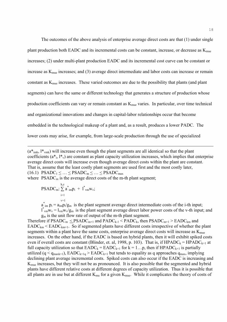
The outcomes of the above analysis of enterprise average direct costs are that (1) under single
plant production both EADC and its incremental costs can be constant, increase, or decrease as Kmue
increases; (2) under multi-plant production EADC and its incremental cost curve can be constant or
increase as Kmue increases; and (3) average direct intermediate and labor costs can increase or remain
constant as Kmue increases. These varied outcomes are due to the possibility that plants (and plant
segments) can have the same or different technology that generates a structure of production whose
production coefficients can vary or remain constant as Kmue varies. In particular, over time technical
and organizational innovations and changes in capital-labor relationships occur that become
embedded in the technological makeup of a plant and, as a result, produces a lower PADC. The
lower costs may arise, for example, from large-scale production through the use of specialized
(a*imk, l*vmk) will increase even though the plant segments are all identical so that the plant coefficients (a*i, l*v) are constant as plant capacity utilization increases, which implies that enterprise average direct costs will increase even though average direct costs within the plant are constant. That is, assume that the least costly plant segments are used first and the most costly later, (16.1) PSADC1 < … < PSADCm < … < PSADCmax where PSADCm is the average direct costs of the m-th plant segment; h,z PSADCm: ∑ a*
impi + l*vmwv;
i=1 v=1 a*
im pi = aimpi/gm is the plant segment average direct intermediate costs of the i-th input; l*
vmwv = lvmwv/gm is the plant segment average direct labor power costs of the v-th input; and gm is the unit flow rate of output of the m-th plant segment. Therefore if PSADCm < PSADCm+1 and PADCk-1 < PADCk, then PSADCm+1 > EADCkm and EADCkm < EADCkm+1. So if segmented plants have different costs irrespective of whether the plant segments within a plant have the same costs, enterprise average direct costs will increase as Kmue increases. On the other hand, if the EADC is based on hybrid plants, then it will exhibit spiked costs even if overall costs are constant (Blinder, et. al, 1998, p. 103). That is, if HPADCk = HPADCk+1 at full capacity utilization so that EADCk = EADCk+1 for k = 1…p, then if HPADCk+1 is partially utilized (q < qmaxk+1), EADCk+1q > EADCk+1 but tends to equality as q approaches qmax, implying declining plant average incremental costs. Spiked costs can also occur if the EADC is increasing and Kmue increases, but they will not be as pronounced. It is also possible that the segmented and hybrid plants have different relative costs at different degrees of capacity utilization. Thus it is possible that all plants are in use but at different Kmu for a given Kmue. While it complicates the theory of costs of
19
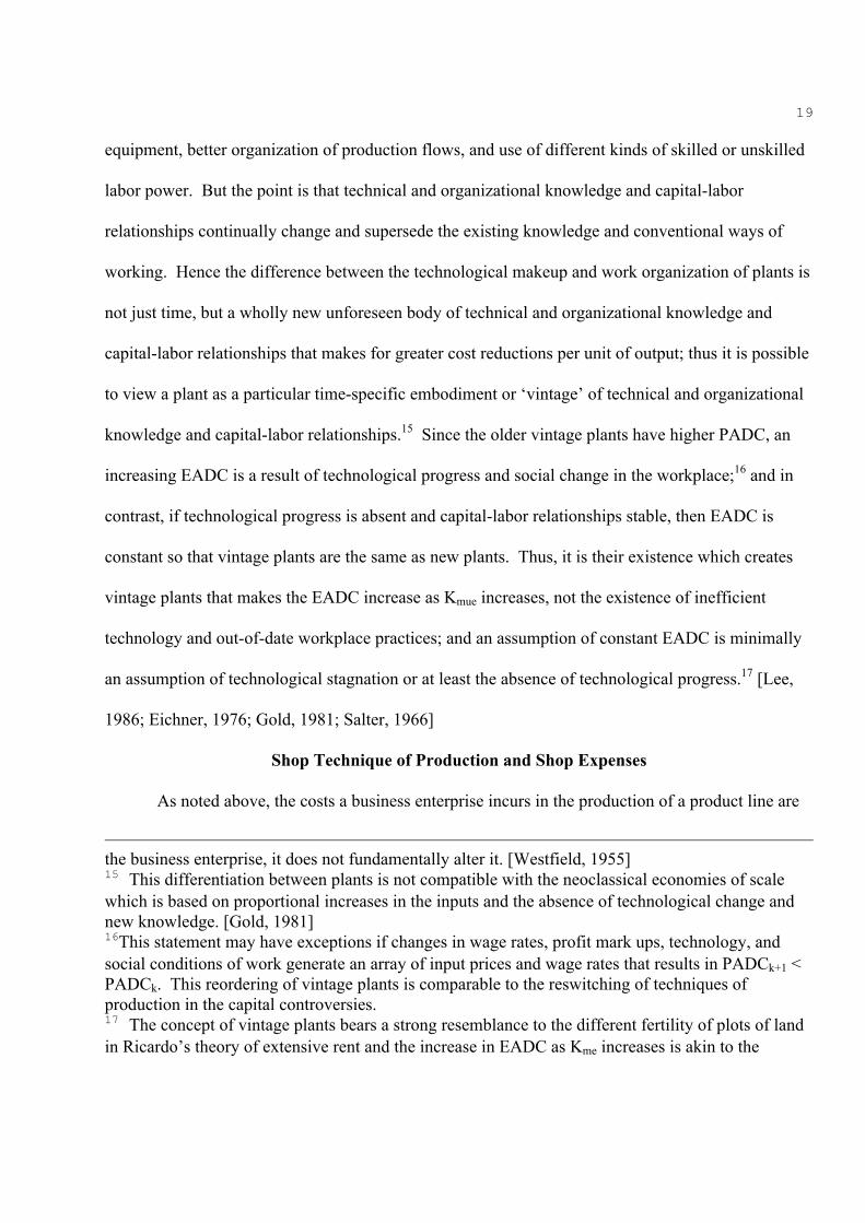
equipment, better organization of production flows, and use of different kinds of skilled or unskilled
labor power. But the point is that technical and organizational knowledge and capital-labor
relationships continually change and supersede the existing knowledge and conventional ways of
working. Hence the difference between the technological makeup and work organization of plants is
not just time, but a wholly new unforeseen body of technical and organizational knowledge and
capital-labor relationships that makes for greater cost reductions per unit of output; thus it is possible
to view a plant as a particular time-specific embodiment or ‘vintage’ of technical and organizational
knowledge and capital-labor relationships.15 Since the older vintage plants have higher PADC, an
increasing EADC is a result of technological progress and social change in the workplace;16 and in
contrast, if technological progress is absent and capital-labor relationships stable, then EADC is
constant so that vintage plants are the same as new plants. Thus, it is their existence which creates
vintage plants that makes the EADC increase as Kmue increases, not the existence of inefficient
technology and out-of-date workplace practices; and an assumption of constant EADC is minimally
an assumption of technological stagnation or at least the absence of technological progress.17 [Lee,
1986; Eichner, 1976; Gold, 1981; Salter, 1966]
Shop Technique of Production and Shop Expenses
As noted above, the costs a business enterprise incurs in the production of a product line are
the business enterprise, it does not fundamentally alter it. [Westfield, 1955] 15 This differentiation between plants is not compatible with the neoclassical economies of scale which is based on proportional increases in the inputs and the absence of technological change and new knowledge. [Gold, 1981] 16This statement may have exceptions if changes in wage rates, profit mark ups, technology, and social conditions of work generate an array of input prices and wage rates that results in PADCk+1 < PADCk. This reordering of vintage plants is comparable to the reswitching of techniques of production in the capital controversies. 17 The concept of vintage plants bears a strong resemblance to the different fertility of plots of land in Ricardo’s theory of extensive rent and the increase in EADC as Kme increases is akin to the
20
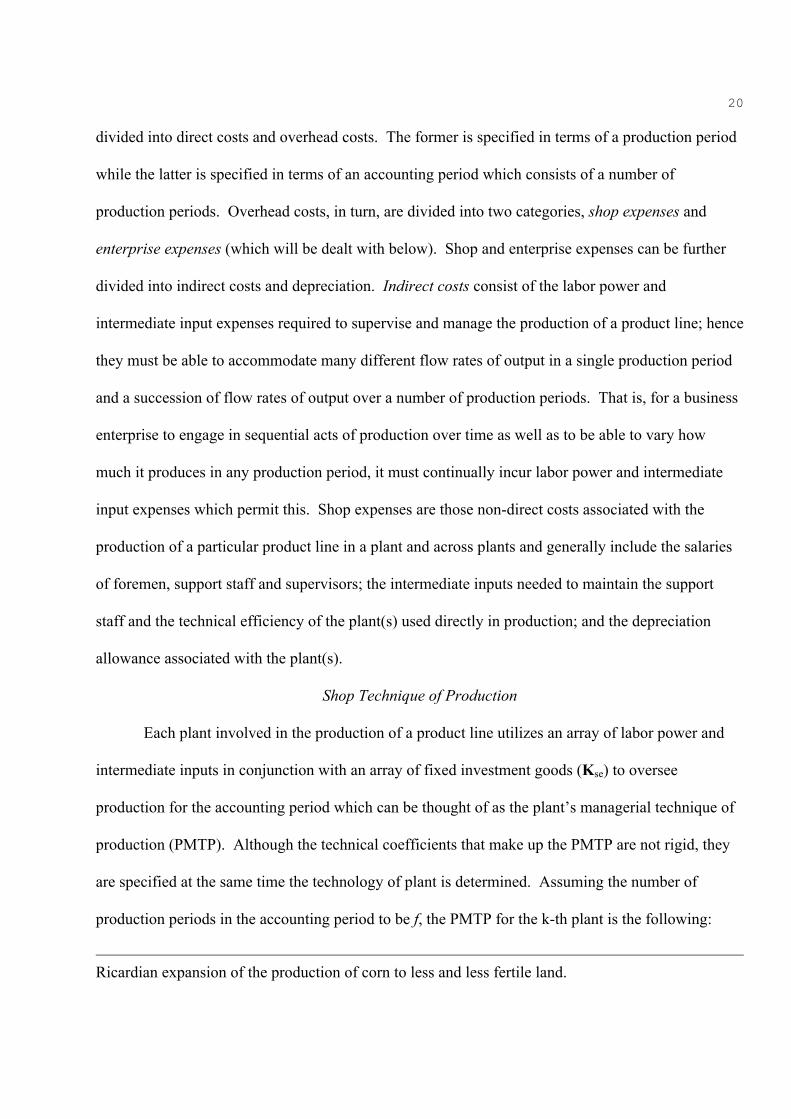
divided into direct costs and overhead costs. The former is specified in terms of a production period
while the latter is specified in terms of an accounting period which consists of a number of
production periods. Overhead costs, in turn, are divided into two categories, shop expenses and
enterprise expenses (which will be dealt with below). Shop and enterprise expenses can be further
divided into indirect costs and depreciation. Indirect costs consist of the labor power and
intermediate input expenses required to supervise and manage the production of a product line; hence
they must be able to accommodate many different flow rates of output in a single production period
and a succession of flow rates of output over a number of production periods. That is, for a business
enterprise to engage in sequential acts of production over time as well as to be able to vary how
much it produces in any production period, it must continually incur labor power and intermediate
input expenses which permit this. Shop expenses are those non-direct costs associated with the
production of a particular product line in a plant and across plants and generally include the salaries
of foremen, support staff and supervisors; the intermediate inputs needed to maintain the support
staff and the technical efficiency of the plant(s) used directly in production; and the depreciation
allowance associated with the plant(s).
Shop Technique of Production
Each plant involved in the production of a product line utilizes an array of labor power and
intermediate inputs in conjunction with an array of fixed investment goods (Kse) to oversee
production for the accounting period which can be thought of as the plant’s managerial technique of
production (PMTP). Although the technical coefficients that make up the PMTP are not rigid, they
are specified at the same time the technology of plant is determined. Assuming the number of
production periods in the accounting period to be f, the PMTP for the k-th plant is the following:
Ricardian expansion of the production of corn to less and less fertile land.
21
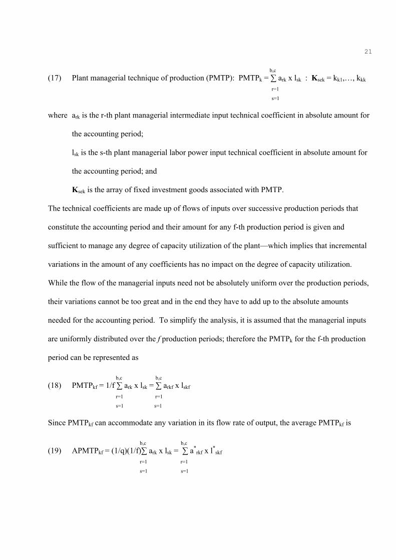
b,c (17) Plant managerial technique of production (PMTP): PMTPk = ∑ ark x lsk : Ksek = kk1,…, kkk r=1 s=1 where ark is the r-th plant managerial intermediate input technical coefficient in absolute amount for the accounting period; lsk is the s-th plant managerial labor power input technical coefficient in absolute amount for the accounting period; and Ksek is the array of fixed investment goods associated with PMTP. The technical coefficients are made up of flows of inputs over successive production periods that
constitute the accounting period and their amount for any f-th production period is given and
sufficient to manage any degree of capacity utilization of the plant—which implies that incremental
variations in the amount of any coefficients has no impact on the degree of capacity utilization.
While the flow of the managerial inputs need not be absolutely uniform over the production periods,
their variations cannot be too great and in the end they have to add up to the absolute amounts
needed for the accounting period. To simplify the analysis, it is assumed that the managerial inputs
are uniformly distributed over the f production periods; therefore the PMTPk for the f-th production
period can be represented as
b,c b,c (18) PMTPkf = 1/f ∑ ark x lsk = ∑ arkf x lskf r=1 r=1 s=1 s=1 Since PMTPkf can accommodate any variation in its flow rate of output, the average PMTPkf is
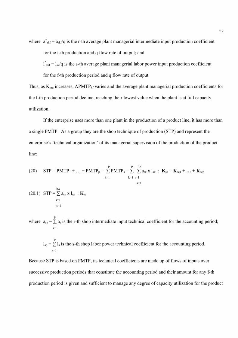
where a*rkf = arkf/q is the r-th average plant managerial intermediate input production coefficient
for the f-th production and q flow rate of output; and l*
skf = lsk/q is the s-th average plant managerial labor power input production coefficient for the f-th production period and q flow rate of output. Thus, as Kmu increases, APMTPkf varies and the average plant managerial production coefficients for
the f-th production period decline, reaching their lowest value when the plant is at full capacity
utilization.
If the enterprise uses more than one plant in the production of a product line, it has more than
a single PMTP. As a group they are the shop technique of production (STP) and represent the
enterprise’s ‘technical organization’ of its managerial supervision of the production of the product
line:
p p b,c (20) STP = PMTP1 + … + PMTPp = ∑ PMTPk = ∑ ∑ ark x lsk : Kse = Kse1 + … + Ksep
k=1
k=1 r=1
s=1 b,c (20.1) STP = ∑ arp x lsp : Kse
r=1 s=1 p where arp = ∑ ar is the r-th shop intermediate input technical coefficient for the accounting period; k=1 p lsp = ∑ ls is the s-th shop labor power technical coefficient for the accounting period. k=1 Because STP is based on PMTP, its technical coefficients are made up of flows of inputs over
successive production periods that constitute the accounting period and their amount for any f-th
production period is given and sufficient to manage any degree of capacity utilization for the product
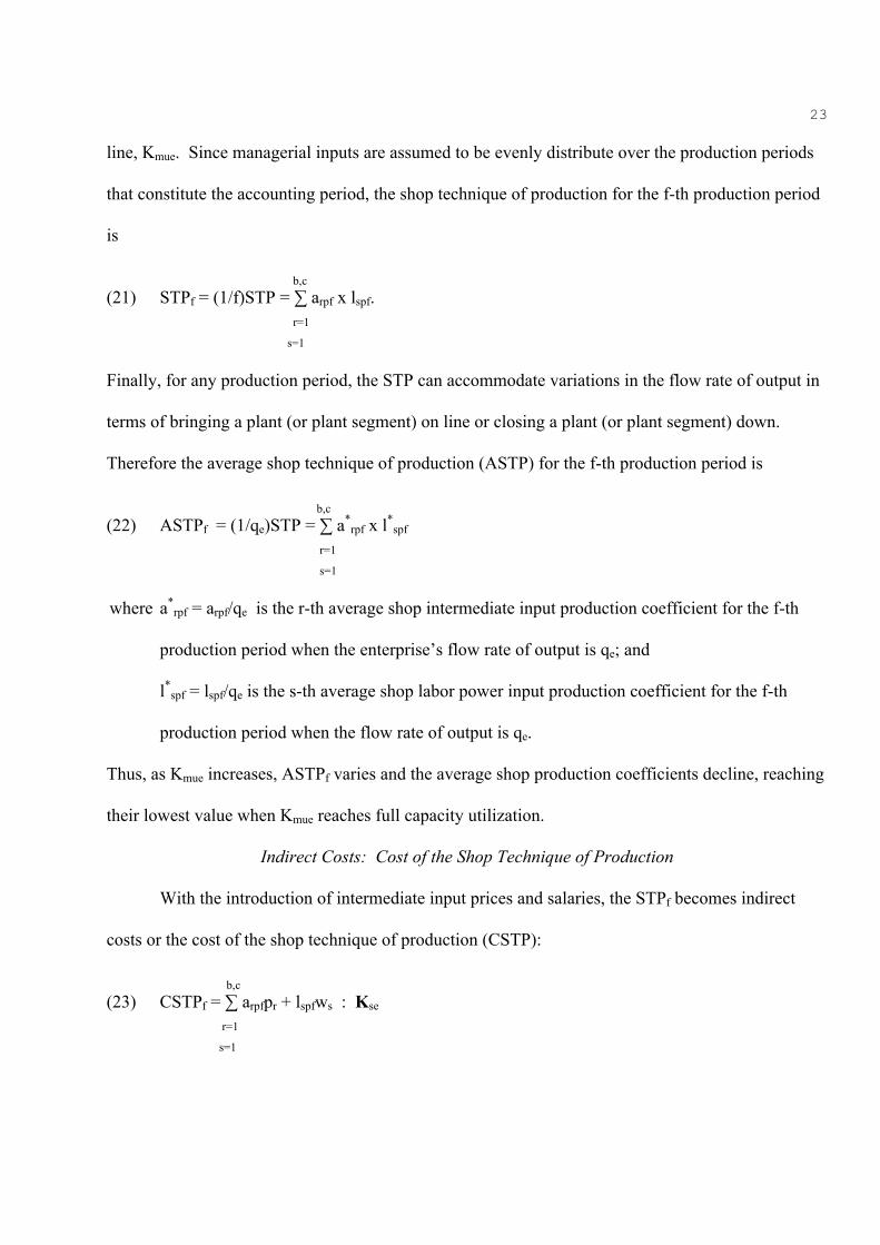
23
line, Kmue. Since managerial inputs are assumed to be evenly distribute over the production periods
that constitute the accounting period, the shop technique of production for the f-th production period
is
b,c (21) STPf = (1/f)STP = ∑ arpf x lspf. r=1
s=1 Finally, for any production period, the STP can accommodate variations in the flow rate of output in
terms of bringing a plant (or plant segment) on line or closing a plant (or plant segment) down.
Therefore the average shop technique of production (ASTP) for the f-th production period is
b,c (22) ASTPf = (1/qe)STP = ∑ a*
rpf x l*spf
r=1 s=1 where a*
rpf = arpf/qe is the r-th average shop intermediate input production coefficient for the f-th production period when the enterprise’s flow rate of output is qe; and l*
spf = lspf/qe is the s-th average shop labor power input production coefficient for the f-th production period when the flow rate of output is qe. Thus, as Kmue increases, ASTPf varies and the average shop production coefficients decline, reaching
their lowest value when Kmue reaches full capacity utilization.
Indirect Costs: Cost of the Shop Technique of Production
With the introduction of intermediate input prices and salaries, the STPf becomes indirect
costs or the cost of the shop technique of production (CSTP):
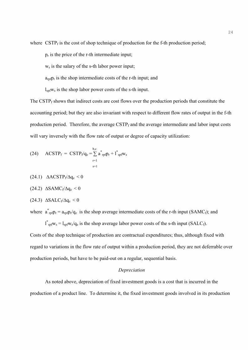
b,c (23) CSTPf = ∑ arpfpr + lspfws : Kse r=1
s=1
24
where CSTPf is the cost of shop technique of production for the f-th production period; pr is the price of the r-th intermediate input; ws is the salary of the s-th labor power input; arpfpr is the shop intermediate costs of the r-th input; and lspfws is the shop labor power costs of the s-th input. The CSTPf shows that indirect costs are cost flows over the production periods that constitute the
accounting period; but they are also invariant with respect to different flow rates of output in the f-th
production period. Therefore, the average CSTPf and the average intermediate and labor input costs
will vary inversely with the flow rate of output or degree of capacity utilization:
rpfpr = arpfpr/qe is the shop average intermediate costs of the r-th input (SAMCf); and l*
spfws = lspfws/qe is the shop average labor power costs of the s-th input (SALCf). Costs of the shop technique of production are contractual expenditures; thus, although fixed with
regard to variations in the flow rate of output within a production period, they are not deferrable over
production periods, but have to be paid-out on a regular, sequential basis.
Depreciation
As noted above, depreciation of fixed investment goods is a cost that is incurred in the
production of a product line. To determine it, the fixed investment goods involved in its production
25
have to be identified. From equations 1, 2, 1.1, 6, 14, 17, and 20, the array of fixed investment goods
associated with the production of the product line is
(25) Kdse = Kd + Kse.
With the fixed investment goods associated with the production of the product line identified, their
individual values are determined based on their historical costs. Then using straight-line or declining
charges methods, the depreciation allowance of each fixed investment good for the accounting period
is determined from whence they are aggregated into a single value amount for the accounting period,
Ddse. Distributing Ddse equally across all production periods, depreciation allowance for the f-th
production period is Ddsef = Ddse/f. Since Ddsef is invariant with respect to variations in the flow rate
of output, average depreciation costs and hence the shop depreciation production coefficient varies
inversely with as the flow rate of output or degree of capacity utilization:
(26) d*dsef = Ddsef/qe
(26.1) ∆d*
dsef/∆qe < 0 where d*
dsef is the shop depreciation production coefficient for the f-th production period when the flow rate of output is qe.
Shop Expenses
Shop expenses (SE) for the f-th production period is obtained by adding together Ddsef and
CSTPf:
b,c (27) SEf = ∑ arpfpr + lspfws + Ddsef. r=1
s=1
Since CSTPf and Ddsef are cost flows, SEf is also a cost flow. Thus it cannot be seen as "fixed" even
though it is invariant with respect to different flow rates of output. Average shop expenses (ASE) for
26
the f-th production period is
b,c (28) ASEf = SEf/qe = ∑ (a*
rpfpr + l*spfws) + d*
dsef : Kse; Kmue r=1 s=1 and as the degree of capacity utilization increases, ASEf declines (equations 24.1 and 26.1)
(28.1) ∆ASEf/∆qe < 0.
Enterprise Technique of Production and Enterprise Expenses
Because the going enterprise is generally a multi-product producer and a going concern, it
incurs expenses that are common to all of its product lines and necessary if it is to stay in existence
as a going concern and hence are identified as enterprise expenses. In general, these costs are
associated with those activities that the enterprise must engage in order to co-ordinate the production
flows of its various product lines, to sell its various product lines, and to develop and implement
enterprise-wide investment and diversification plans and which include the salaries of management,
stationary, selling and other office expenses, and the depreciation of the central office fixed
investment goods. This array of labor power and intermediate inputs in conjunction with an array of
fixed investment goods (Kee = kee1,…, keek) are used to manage the enterprise as a whole for the
accounting period which includes the various degrees of capacity utilization for any one product line
and all product lines; and it can be thought of as the enterprise technique of production (ETP):
o,y (29) ETP = ∑ au x le : Kee
u=1 e=1 where au is the u-th enterprise intermediate input technical coefficient for the accounting period; and le is the e-th enterprise labor power technical coefficient for the accounting period. The technical coefficients are made up of flows of inputs over the accounting period that are not
27
synchronized with the production periods of the various production lines, which would not be
possible in any case since they are not necessarily the same. Therefore, it is not possible, as with the
STP, to allocate the flow of the inputs to any and all product lines; rather the allocation is done in
terms of money.
With the introduction of intermediate input prices and yearly salaries, the ETP becomes
indirect costs or the cost of the enterprise technique of production (CETP):
o,y (30) CETP = ∑ aupu + lese u=1 e=1 where pu is the input price of the u-th enterprise intermediate input; aupu is the enterprise intermediate costs for the u-th input for the accounting period; se is the yearly salary of the e-th labor power input; and lese is the enterprise labor power costs for the e-th input for the accounting period. Given the CETP for the accounting period, it is allocated to each of the enterprise’s j product lines.
Once a given percentage of CETP, αCETP, is allocated to the j-th product line for the accounting
period, it is then allocated equally over all the production periods. Therefore, the CETP for the
enterprise’s j-th product line and the f-th production period is
o,y o,y (31) CETPjf = (αj)(1/f)(∑ aupu + lese) = ∑ aujfpu + lejfse u=1 u=1 e=1 e=1 where aujfpu is the enterprise intermediate costs for the u-th input for the j-th product line and f-th production period; lejfse is the enterprise labor power costs for the e-th input for the j-th product line and f-th production period; and
28
αj is the percentage of CETP allocated to the j-th product line. Like with the CSTPf, the CETPjf shows that indirect costs are cost flows over the production periods
that constitute the accounting period; but they are also invariant with respect to different flow rates of
output in the f-th production period. Therefore, the average CETPjf and the average intermediate and
labor input costs will vary inversely with the flow rate of output or degree of capacity utilization:
ujfpr = aujfpr/qje is the enterprise average intermediate costs of the u-th input of the j-th product line (EAMCjf); and l*
ejfws = lejfws/qje is the enterprise average labor power costs of the e-th input of the j-th product line (EALCjf). Costs of the enterprise technique of production are also contractual expenditures: thus, although
fixed with regard to variations in the flow rate of output within a production period, they are not
deferrable over production periods, but have to be paid-out on a regular, sequential basis.
Because the array of fixed investment goods (Kee = kee1,…, keek) associated with the ETP are
known, the depreciation allowance for enterprise expenses, De, for the accounting period is
determined in the same manner described above in reference to shop expenses. It is then allocated to
the various product lines so that the enterprise depreciation allowance of the j-th product line for the
accounting period is Dej = (αj)(De); and for the j-th product for the f-th production period, it is Dejf =
29
(1/f)(αj)(De). Finally, although Dejf is invariant with respect to variations in the flow rate of output,
the enterprise depreciation production coefficient for the j-th product line and f-th production period
varies as the flow rate of output varies:
(32) d*ejf = Dejf/qje
(32.1) ∆d*
ejf/∆qje < 0 where d*
ejf is the enterprise depreciation production coefficient of the j-th product line for the f-th production period when the flow rate of output is qje. Finally, the enterprise expenses for the accounting period consist of the cost of the enterprise
technique of production and depreciation; thus the enterprise expenses (EE) for the j-th product line
in the f-th production period is
o,y (33) EEjf = CETPjf + Dejf = ∑ aujfpu + lejfse + Dejf. u=1 e=1 Since each of its components are cost flows, the EEjf is also a cost flow. Thus it cannot be seen as
"fixed" even though it is invariant with respect to different flow rates of output. Average enterprise
expenses for the j-th product line and f-th production period is
o,y (34) AEEjf = EEjf/qje = ACETPjf + d*
ejf = ∑ (a*ujfpu + l*
ejfse) + d*ejf : Kee; Kmue
u=1 e=1
and as the degree of capacity utilization increases, AEEjf declines (equations 31.1 and 32.1)
(34.1) ∆AEEjf/∆qje < 0.
Structure of Production and Costs of a Product Line
The average structure of production for the business enterprise’s j-th product line in terms of
the f-th production period and for a flow rate of output of qje (derived from equations 14, 22, and 31)
30
Structure of Production for a Product (SPP)
h,b,o,z,c,y (35) ASPPjf = ∑ a*
ijf x a*rjf x a*
ujf x l*vjf x l*
sjf x l*ejf : Kz = Kd + Kse + Kee; Kmue
i=1 r=1
u=1
v=1
s=1
e=1
Equation 35 clearly shows that the enterprise’s SPP consists of an array of material and service
inputs and labor power (skills) whose production coefficients are jointly determined by technology
and the flow rate of output. So while the structure itself remains stable in face of variations of the
flow rate of output, the production coefficients can vary: (1) a*rjf, a*ujf, l*sjf, and l*ejf all decline as
the flow rate of output (qje) increases; and (2) a*ijf and l*
vjf can remain constant or increase as output
increases. Hence the SPP changes only when the underlying technology and social/labor
relationships change, resulting in changes in changing the material and labor power inputs. This
generally occurs when new plants (or plant segments) are brought on line and as vintage plants (plant
segments) are dropped as well as when managerial and enterprise techniques of production are
altered; but it can also occur after a failed (or successful) strike.
When considering the structure of costs for a single product, we are essentially considering
the enterprise’s average total costs of production for the j-th product line, f-th production period, and
flow rate of output of qje:
(36) Enterprise average total costs of production for the j-th product line (EATCj)—see equations
e=1 where EADCjf is the enterprise average direct costs for the j-th product line, f-th production period when the flow rate of output is qje; ASEjf is the average shop expenses for the j-th product line, f-th production period when the flow rate of output is qje; and AEEjf is the average enterprise expenses for the j-th product line, f-th production period when the flow rate of output is qje. Restricting the structural analysis to a single production period, the relationship between EATCjf and
the flow rate of output can be shown in the following manner:
(37) ∆EATCjf > 0 if PADCjk+1 > EATCjf ∆qje = 0 if PADCjk+1 = EATCjf < 0 if PADCjk+1 < EATCjf. Thus we find that the specific forms of the relationship depend on a tug-of-war between the rising
incremental costs and the falling ASEjf and AEEjf. Since there is no necessary reason for the relative
dominance of one side over the other, a positive, negative, or U-shaped EATCjf are possible. The
empirical evidence does suggest, however, that EATCjf is declining as the flow rate of output
increases. Still, it should be noted that whatever the shape of the average total cost curve is, the
shape is solely due to technological and organizational change and changes in capital-labor
relationships and hence is solely an empirical issue. [Insert data reference]
Conclusion
32
The beginning point of heterodox production and cost theory is not the business enterprise
per se, but a circular production, surplus producing economy. For such an economy, production and
the surplus are delineated in terms of an Leontief-Sraffa input-output model complete with industry
or market level production coefficients. However, what is lacking is a connection between the
business enterprise which actually does the production and the industry level coefficients. The
heterodox theory of production and costs of an enterprise’s product line delineated above fills this
gap by developing the theoretical ‘micro’ foundations of the industry production coefficients that
consisted of a product-based input-output structure, an explanation of the movements of production
coefficients, and finally an explanation of average and incremental cost curves. Given this, how does
heterodox production and cost theory stand relative to neoclassical theory? Because it is based on
the going business enterprise with its relatively enduring (but not unchanging) accounting rules and
unceasing sequential acts of production, the theory cannot be located in the short or long period.
Rather the relevant time periods for theoretical purposes are the production period and the
accounting period, both of which are calendar time/real time periods and not solely analytical time
periods defined in terms of fixed and variable inputs. The going enterprise is also predicated on
reproducible, differentiated intermediate inputs and differentiated labor power, implying the rejection
of inputs being characterized as relatively scarce factors of production and of the ‘linear’ reduction
of intermediate inputs to an objective or subjective quantity of homogeneous labor power or effort.
Finally, the role of a going enterprise’s accounting rules in determining what constitutes the
reoccurring costs of a product line makes costs a socially constructed concept as opposed to an
unambiguous, unmediated objective concept. These three points fundamentally differentiate
heterodox from neoclassical production and cost theory: the former is in the theoretical universe of
historical time, reproducible inputs, non-reductionism, and social knowledge whereas the latter is in
33
a universe of analytical time, relative scarcity, reductionism, and socially unmediated knowledge.
Heterodox theory also differs from neoclassical theory on the particulars. That is, the
heterodox characterization of production as a recipe embedded in a plant is incompatible with
intensive rent qua the productivity of individual inputs qua marginal products, fixed-variable input
distinction, and the full utilization of a fixed input requirement for the existence of marginal
products; and without marginal products (and relative scarcity), the law of diminishing returns does
not exist as well as cost minimization, marginal cost curves and their upward slope, the marginal rate
of technical substitution, and constant output factor input demand curves. Since vintage plants differ
by knowledge and capital-labor relationships that are historically contingent, factor substitution via
changes in relative factor input prices, and returns to scale have no substantive meaning. Finally, the
inclusion of depreciation solely as a money cost and the rejection of the rate of interest or normal
profits as a cost make the meaning of heterodox and neoclassical average total costs quite different.
Therefore, the choice between neoclassical and heterodox production and cost theory is based on the
empirical validity and theoretical superiority of the latter.
Although fundamentally different at the theoretical level, heterodox and neoclassical
production and cost theory are similarly organized. Both theories start with a structure of production
in which inputs are connected to outputs, although the actual production processes are left
unarticulated; and from the structures, the movement of production coefficients (average products)
and ‘incremental’ plants (marginal products) are delineated. In short, both theories see production as
a technological, organizational, and (at least for heterodox economists) social activity central to
understanding the business enterprise. The transformation of production into costs is carried out in a
similar manner by both theories, giving rise to similar looking cost curves. Since their theoretical
content is, for both theories, located in the theory of production, the curves superficial resemblance
34
obscures their profound theoretical differences. This tight connection between production and cost
theory means for both theories that it is illegitimate to discuss the costs of the business enterprise
independent of its structure of production. This point can be further extended for heterodox
economics in that it is illegitimate to aggregate structures of production and costs across product
lines. That is, heterodox production and cost theory is predicated on an input-output relationship of a
well-defined product line. So long as the production of the goods and services needed for social
provisioning require distinct and differentiated reproducible inputs, labor power inputs, and fixed
investment goods, it is not possible to aggregate the different product lines and their corresponding
structures of production into a single homogeneous input-output (such as in a corn model or a labor-
based production model). Therefore the input-output relationship is the foundation of both the going
capitalist economy and the going business enterprise. From this, it can be inferred that production
and cost theory provides, in part, the foundation from which all heterodox theory emanates.
References
Al-Omiri, M. and Drury, C. (2007) ‘A Survey of Factors Influencing the Choice of Product Costing
Systems in UK Organizations’, Management Accounting Research 18: 399-424.
Blinder, A. S., Canetti, E. R. D., Lebow, D. E., and Rudd, J. B. 1998. Asking About Prices: a new
approach to understanding price stickiness, New York: Russell Sage Foundation.
Boyns, T. and Edwards, J. R. (1995) ‘Accounting Systems and Decision-Making in the Mid-
Victorian Period: the case of the Consett Iron Company’, Business History, 37(3): 28–51.
__________ (1997) ‘The Construction of Cost Accounting Systems in Britain to 1900: the case of
the coal, iron and steel industries’, Business History, 39(3): 1-29.
35
Boyns, T., Edwards, J. R., and Nikitin, M. (1997) The Birth of Industrial Accounting in France and
Britain, New York: Garland Publishing, Inc.
Bright. J., Davies, R. E., Downes, C. A., and Sweeting, R. C. (1992) ‘The Deployment of Costing
Techniques and Practices: a UK study’, Management Accounting Research, 3(3): 201-11.
Chatfield, M. (1974) A History of Accounting Thought, Hinsdale: The Dryden Press.
Dean, J. (1976) Statistical Cost Estimation, Bloomington: Indiana University Press.
Edwards, J. R. (1980) ‘British Capital Accounting Practices and Business Finance 1852-1919: an
exemplification’, Accounting and Business Research, 10: 241-58.
Edwards, J. R. (1986) ‘Depreciation and Fixed Asset Valuation in British Railway Company
Accounts to 1911’, Accounting and Business Research, 16: 251-63.
Edwards, J. R. (1989) ‘Industrial Cost Accounting Developments in Britain to 1830: a review
article’, Accounting and Business Research, 19(76): 305-17.
Eichner, A. S. (1976) The Megacorp and Oligopoly. New York City: Cambridge University Press.
Emore, J. R., and J. A. Ness. 1991. “The Slow Pace of Meaningful Change in Cost Systems,”
Journal of Cost Management, 5(4): 36-45.
Fleischman, R. K. and Parker, L. D. (1997) What is Past is Prologue: cost accounting in the British
industrial revolution, 1760–1850, New York: Garland Publishing, Inc.
Garner, S. P. (1954) Evolution of Cost Accounting to 1925. University: The University of Alabama
Press.
Gold, B. (1981) ‘Changing Perspectives on Size, Scale, and Returns: an interpretive survey’, The
Journal of Economic Literature 19(1): 5-33.
Granlund, M. (2001) ‘Towards Explaining Stability in and Around Management Accounting
36
Systems’, Management Accounting Research 12: 141-66.
Hudson, P. (1977) ‘Some Aspects of 19th Century Accounting Development in the West Riding
Textile Industry’, Accounting History, 2: 4–22.
Jones, H. (1985) Accounting, Costing and Cost Estimation: Welsh industry 1700-1830. Cardiff:
University of Wales Press.
Kurz, H. and Salvadori, N. (2005) ‘Representing the Production and Circulation of Commodities in
Material Terms: on Sraffa’s objectivism’, Review of Political Economy, 17(3): 413–41.
Lee, F. S. (1986) ‘Post Keynesian View of Average Direct Costs: a critical evaluation of the theory
and the empirical evidence‘, Journal of Post Keynesian Economics, 8: 400–24.
______ (1998) Post Keynesian Price Theory, Cambridge: Cambridge University Press.
Litherland, D. A. (1951) ‘Fixed Asset Replacement a Half Century Ago’, The Accounting Review,
26(4): 475-80.
Lukka, K. (2007) ‘Management Accounting Change and Stability: loosely coupled rules and routines
in action’, Management Accounting Research, 18(1): 76-103.
Napier, C. J. (1990) ‘Fixed Asset Accounting in the Shipping Industry: P&O 1840-1914’,
Accounting, Business and Financial History 1(1): 23-50.
Salter, W. E. G. (1966) Productivity and Technical Change, 2nd edn, Cambridge: Cambridge
University Press.
Stone, W. E. (1973-74) “An Early English Cotton Mill Cost Accounting System: Charlton Mills,
1810-1889’, Accounting and Business Research, 4: 71-8.
Tyson, T. (1992) ‘The Nature and Environment of Cost Management Among Early Nineteenth
Century U.S. Textile Manufacturers’, The Accounting Historians Journal, 19(2): 1-24.
37
Wale, J. (1990) ‘The Reliability of Reported Profits and Asset Values, 1890-1914: case studies from
the British coal industry’, Accounting and Business Research, 20(79): 253-67.
Westfield, F. M. (1955) ‘Marginal Analysis, Multi-Plant Firms, and Business Practice: an example’,
The Quarterly Journal of Economics, 69(2): 253-68.