International Economic JournalVol. 24, No. 2, 255–282, June 2010
Heterogeneity in Ability andInheritance, Disparities, and
Development
SHERIF KHALIFA
Department of Economics, California State University, Fullerton, California, USA
(Received 18 February 2008; accepted 14 October 2009)
ABSTRACT This paper investigates the impact of income inequality on economic growth.A two-period overlapping generations model is developed where agents are heterogeneousin innate abilities and inheritance. In the first period, they receive their inheritance and theirabilities are revealed. There are only two types of abilities: high and low. Individuals decideon their education level, and divide their inheritance between spending on education andsaving. In the second period, individuals supply their labor and allocate the labor incomeand the return to their saving between consumption and bequests to their offsprings. Initialcapital stock is owned entirely by the capitalists. In this context, a more equal distributionof income enhances economic growth if the economy is lower than a threshold capital-labor ratio, while income inequality has an insignificant effect above this threshold. Thepredictions of the model are tested empirically using the Hansen (1999) threshold estimation.The results, using a panel of 70 countries for the period 1971-1999, suggest that there isa statistically significant threshold income per capita, below which the coefficient on therelationship between inequality and economic growth is significantly negative and abovewhich the estimate is not significant.
KEY WORDS: Income inequality, economic growthJEL CLASSIFICATIONS: D9, D31
1. Introduction
The distribution of income in an economy, and its effect on economic outcomes,has always been a source of concern for economists. In this context, there are two
Correspondence Address: Sherif Khalifa, Department of Economics, California State University,Fullerton, CA, 92834, USA. Email: [email protected]
streams of literature. One argues that income inequality is propitious to economicperformance, while the other concludes that the prevalent disparities call for anintervention to achieve the desired outcomes. According to Kuznets (1955), theseattempts struggled in a ‘field of study that has been plagued by looseness indefinitions, unusual scarcity of data, and pressure of strongly held opinions’.
On one hand, a vast literature argues that greater egalitarian conditions are aprerequisite for economic growth, and that inequality adversely affects the overallperformance of the economy. For instance, Barro (2000) shows that redistributionfrom the rich whose marginal productivity is low to the poor whose marginal pro-ductivity is high, but cannot invest in human capital more than their endowmentdue to capital market imperfections, would enhance productivity and growth.
From a political economy point of view, Persson and Tabellini (1994) showthat in more inegalitarian economies a majority of voters prefer a higher level ofredistribution, which reduces the incentives for investment. Alesina and Rodrick(1994) demonstrate that the more equitable the economy the better endowed themedian voter with capital, and thus the lower the level of capital taxation andthe higher is the economy’s growth. Finally, Perotti (1992, 1993) emphasizes thatincome disparities motivate disruptive and destabilizing activities, and argues thatredistributive policies reduce social tension.
Another stream of literature disputes the previous conclusions and asserts thatthe skewness of the income distribution is conducive to economic performance.In support of this opinion, Forbes (2000) provides empirical evidence that incomeinequality has a significant positive effect on economic growth. In this context,studies of consumption and saving behavior proposed a channel in which inequal-ity has a stimulating effect on growth. For instance, Carroll (2000) finds that themarginal propensity to save of the rich is higher than that of the poor. This isbecause, according to the precautionary saving incentive, consumers with smallasset stocks tend to compress their consumption so that their marginal propensityto consume out of wealth is higher than that of those holding larger asset stocks.The implication is that if the growth rate of income is proportional to aggregatesaving, then more inegalitarian economies grow faster.
As an attempt to reconcile these two streams, Galor and Moav (2004) providea unified approach that argues that, in the early stages of development, physicalcapital accumulation is the primary source of economic growth. Thus, inequalityenhances growth by channeling resources towards individuals whose marginalpropensity to save is higher. In later stages of development, physical capital isreplaced by human capital as the engine of growth. Accordingly, equality allevi-ates the adverse effects of credit constraints on human capital accumulation andprompts the growth process.
This paper extends the framework in Galor and Moav (2004) by introducingagent heterogeneity across innate abilities and inheritance. This is to emphasizethat what generates income inequality is not only differences in what one inher-its but also differences in one’s ability to generate income through labor. Thisextension suggests that a more equitable income distribution enhances economicgrowth at an earlier stage than the one proposed by Galor and Moav (2004).
An overlapping generations framework is developed in which individuals livefor two periods. In the first period, they receive their inheritance and their innate
Heterogeneity in Ability and Inheritance, Disparities, and Development 257
abilities are revealed. The term inheritance is used interchangeably with bequestsreceived from parents in this context. Individuals decide on their optimal educa-tion level, and divide their inheritance between spending on education and savingfor the second period, and then devote their entire time to the acquisition ofhuman capital. In the second period, individuals supply their efficiency units oflabor and allocate the resulting labor income along with the return to their sav-ing between consumption and bequests to their offsprings. Initial capital stockis entirely owned by a proportion of the population referred to as capitalists,while the remainder are referred to as workers. There are only two types of innateabilities: high and low. In this context, a more equitable distribution of incomeenhances economic growth if the economy is lower than a threshold capital-laborratio, while income inequality has an insignificant effect above this threshold. Thepredictions of the model are tested empirically using the Hansen (1999) thresholdestimation. The results, using a panel of 70 countries for the period 1971-1999,suggest that there is a statistically significant threshold income per capita, belowwhich the coefficient on the relationship between inequality and economic growthis significantly negative and above which the estimate is not significant.
The remainder of the paper is organized as follows: section 2 includes themodel, section 3 includes the empirical estimation, section 4 is the conclusion.Data and derivations are given in the appendices.
2. Model
Consider an overlapping generations economy in which economic activity extendsover an infinite discrete time. In every period, a generation of measure 1 is born.
2.1 Firms
In every period, the economy produces a single homogeneous good. The factorsof production are physical capital and human capital. The stock of physicalcapital in every period is the output produced in the preceding period net ofconsumption and human capital investment. The level of human capital in everyperiod is a function of individuals’ education decisions in the previous period.Output is produced at time t according to a neoclassical constant returns to scaleproduction technology as follows:
Yt = Y(Kt, Ht) = AH1−αt Kα
t (1)
where A is the level of technology,1 and α ∈ (0, 1). Kt = ∫ 10 Sit−1di is the quantity
of physical capital in efficiency units employed in production in period t, and isthe sum of the saving Sit−1 of all individuals in period t − 1. Ht = ∫ 1
0 Hit−1di is
1The introduction of technological progress that is fueled by human capital accumulation wouldnot affect the qualitative results. If human capital accumulation is conducive for economic growth,the optimal evolution of the economy would require the fastest physical capital accumulation inearly stages of development so as to raise the incentive to invest in human capital. Inequality inearly stages would therefore stimulate the process of development.
258 S. Khalifa
the quantity of human capital in efficiency units employed in production in periodt, and is the sum of the human capital acquired by all individuals in period t − 1.Firms operate in a perfectly competitive environment. Given the wage rate perefficiency units of labor Wt and the rate of return to capital Rt, firms in period tchoose the level of employment of physical and human capital so as to maximizetheir profits
{Kt, Ht} = argmax[AH1−αt Kα
t − WtHt − RtKt] (2)
The firms demand the optimal level of physical capital, such that the return tophysical capital is equal to its marginal productivity
Rt = AαH1−αt Kα−1
t = Aα(kt)α−1 = R(kt) (3)
The firms demand the optimal level of human capital, such that the return tohuman capital is equal to its marginal productivity
Wt = A(1 − α)H−αt Kα
t = A(1 − α)(kt)α = W(kt) (4)
where kt =(
KtHt
)is the capital-labor ratio, ∂Rt
∂kt= Aα(α − 1)kα−2
t < 0, and∂Wt∂kt
= A(1 − α)αkα−1t > 0. The first derivative ensures that physical capital is
the engine for growth at an early stage of development when kt is small. The lastderivative emphasizes that the accumulation of physical capital increases the rateof return to human capital, and thus induces human capital accumulation.
2.2 Individuals
In every period, a generation that consists of a continuum of individuals ofmeasure 1 is born. Each individual has a single parent and a single offspring.Individuals live for two periods. In the first period of their lives, they receive theirinheritance and their abilities are revealed. For simplicity, we assume there aretwo types of innate abilities: high ability and low ability. Individuals decide ondividing their inheritance between spending on education and saving for the sec-ond period, and then devote their entire time to the acquisition of human capital.The consumption of an individual in the first period can be perceived as part ofthat of the parent. In the second period, individuals supply their efficiency unitsof labor and allocate the resulting labor income along with the return to theirsaving between consumption and bequests to their offsprings.
2.2.1 Second period. Individuals, within as well as across generations, areidentical in their preferences. For individual i, preferences are represented bya log-linear utility function2 over consumption during adulthood Cit+1, and the
2This formulation is common in the literature and suggests that individuals are ex-ante identicalin their intertemporal preferences, although due to differences in income their marginal propensityto save may differ. This form is supported empirically by Altonji et al. (1997).
Heterogeneity in Ability and Inheritance, Disparities, and Development 259
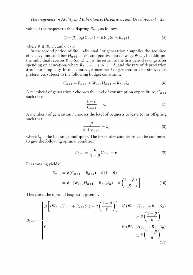
value of the bequest to the offspring Bit+1 as follows:
(1 − β) log(Cit+1) + β log(θ + Bit+1) (5)
where β ∈ (0, 1), and θ > 0.In the second period of life, individual i of generation t supplies the acquired
efficiency units of labor Hit+1, at the competitive market wage Wt+1. In addition,the individual receives Rt+1Sit, which is the return to the first period savings afterspending on education, where Rt+1 = 1 + rt+1 − δ, and the rate of depreciationδ = 1 for simplicity. In this context, a member i of generation t maximizes hispreferences subject to the following budget constraint:
Cit+1 + Bit+1 ≤ Wt+1Hit+1 + Rt+1Sit (6)
A member i of generation t chooses the level of consumption expenditure, Cit+1such that:
1 − β
Cit+1= λt (7)
A member i of generation t chooses the level of bequests to leave to his offspringsuch that:
β
θ + Bit+1= λt (8)
where λt is the Lagrange multiplier. The first-order conditions can be combinedto give the following optimal condition:
Bit+1 = β
1 − βCit+1 − θ (9)
Rearranging yields:
Bit+1 = β(Cit+1 + Bit+1) − θ(1 − β)
= β
[(Wt+1Hit+1 + Rt+1Sit) − θ
(1 − β
β
)](10)
Therefore, the optimal bequest is given by:
Bit+1 =
⎧⎪⎪⎪⎪⎪⎪⎪⎪⎪⎨⎪⎪⎪⎪⎪⎪⎪⎪⎪⎩
β
[(Wt+1Hit+1 + Rt+1Sit) − θ
(1 − β
β
)]if (Wt+1Hit+1 + Rt+1Sit)
> θ
(1 − β
β
)
0 if (Wt+1Hit+1 + Rt+1Sit)
≤ θ
(1 − β
β
)(11)
260 S. Khalifa
2.2.2 First period. The innate ability of each individual is revealed at thebeginning of the first period of their lives, and they devote their entire time tothe acquisition of human capital. The acquired level of human capital increasesif their time investment is supplemented by capital investment. The bequestsreceived from parents are allocated between the finance of education Eit andsaving, thus Sit = Bit − Eit. We also assume that individuals cannot borrow tofinance education.
As the indirect utility function is a strictly increasing function of the individuals’second period wealth, individual i chooses the optimal level of education Lit so asto maximize the second period wealth, Wt+1Hit+1 + Rt+1Sit. This is subject tothe efficiency units of labor that a member i of generation t supplies in the secondperiod, which is a strictly increasing, strictly concave function of the individual’slevel of education in period t; Hit+1 = H(Lit). In the absence of expenditureon education, individuals acquire one efficiency unit of labor as basic skills;H(0) = 1. This assumption is intended to allow those who do not receive bequests,and cannot spend on education, to receive labor income. This income increaseswith the increase in wages due to the increase in the capital-labor ratio until itcrosses the threshold ((θ(1 − β))/β), after which they can leave bequests to theiroffsprings. Also assume that lim
Lit→0H′(Lit) = γ < ∞, and lim
Lit→∞ H′(Lit) = 0. The
expenditure on education is given by:
Eit = jLit (12)
where j; j ∈ (h, l) for high and low ability respectively, is the cost of a unit ofeducation, such that h < l. This can be perceived as a reduction in the cost ofeducation due to the ease with which high-ability individuals absorb the subjectthey are learning compared with low-ability ones. The optimal level of educationis thus the solution to:
Lit+1 = argmax[Wt+1H(Lit) + Rt+1(Bit − Eit)] (13)
The optimal level of education of individual i of generation t is chosen such that:
H′(Lit) = Rt+1
Wt+1j = R(Kt+1)
W(kt+1)j (14)
This means that the optimal level of education is unique and identical across thoseof the same ability category of generation t. Thus, the optimal education levelfor an individual i amongst those with high ability is given by Lh
t = Lh(h, kt+1),and for individual i amongst those with low ability is given by Ll
t = Ll(l, kt+1).Accordingly, the optimal expenditure on education is also identical across thoseof the same ability, such that Eh
t = hLht and El
t = lLlt.
Proposition 1 ∃ a unique capital labor ratio kj = α(1−α)γ
j; j ∈ (h, l), belowwhich individuals with innate ability j do not invest in human capital, and such
Heterogeneity in Ability and Inheritance, Disparities, and Development 261
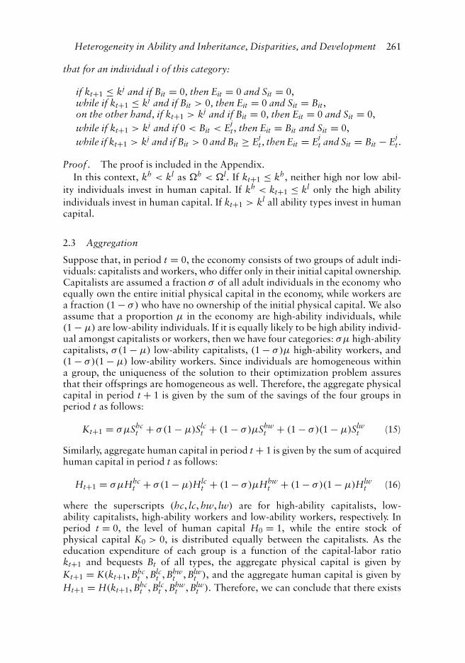
that for an individual i of this category:
if kt+1 ≤ kj and if Bit = 0, then Eit = 0 and Sit = 0,while if kt+1 ≤ kj and if Bit > 0, then Eit = 0 and Sit = Bit,on the other hand, if kt+1 > kj and if Bit = 0, then Eit = 0 and Sit = 0,while if kt+1 > kj and if 0 < Bit < Ej
t, then Eit = Bit and Sit = 0,while if kt+1 > kj and if Bit > 0 and Bit ≥ Ej
t, then Eit = Ejt and Sit = Bit − Ej
t.
Proof. The proof is included in the Appendix.In this context, kh < kl as h < l. If kt+1 ≤ kh, neither high nor low abil-
ity individuals invest in human capital. If kh < kt+1 ≤ kl only the high abilityindividuals invest in human capital. If kt+1 > kl all ability types invest in humancapital.
2.3 Aggregation
Suppose that, in period t = 0, the economy consists of two groups of adult indi-viduals: capitalists and workers, who differ only in their initial capital ownership.Capitalists are assumed a fraction σ of all adult individuals in the economy whoequally own the entire initial physical capital in the economy, while workers area fraction (1 − σ) who have no ownership of the initial physical capital. We alsoassume that a proportion μ in the economy are high-ability individuals, while(1 − μ) are low-ability individuals. If it is equally likely to be high ability individ-ual amongst capitalists or workers, then we have four categories: σμ high-abilitycapitalists, σ(1 − μ) low-ability capitalists, (1 − σ)μ high-ability workers, and(1 − σ)(1 − μ) low-ability workers. Since individuals are homogeneous withina group, the uniqueness of the solution to their optimization problem assuresthat their offsprings are homogeneous as well. Therefore, the aggregate physicalcapital in period t + 1 is given by the sum of the savings of the four groups inperiod t as follows:
Kt+1 = σμShct + σ(1 − μ)Slc
t + (1 − σ)μShwt + (1 − σ)(1 − μ)Slw
t (15)
Similarly, aggregate human capital in period t + 1 is given by the sum of acquiredhuman capital in period t as follows:
Ht+1 = σμHhct + σ(1 − μ)Hlc
t + (1 − σ)μHhwt + (1 − σ)(1 − μ)Hlw
t (16)
where the superscripts (hc, lc, hw, lw) are for high-ability capitalists, low-ability capitalists, high-ability workers and low-ability workers, respectively. Inperiod t = 0, the level of human capital H0 = 1, while the entire stock ofphysical capital K0 > 0, is distributed equally between the capitalists. As theeducation expenditure of each group is a function of the capital-labor ratiokt+1 and bequests Bt of all types, the aggregate physical capital is given byKt+1 = K(kt+1, Bhc
t , Blct , Bhw
t , Blwt ), and the aggregate human capital is given by
Ht+1 = H(kt+1, Bhct , Blc
t , Bhwt , Blw
t ). Therefore, we can conclude that there exists
262 S. Khalifa
a continuous single valued function, such that the capital-labor ratio in periodt + 1 is fully determined by the level of bequests of all types
kt+1 = k(Bhct , Blc
t , Bhwt , Blw
t ), (17)
where k0 ∈ (0, kh). This assumption ensures that in the initial stages the rate ofreturn to physical capital is higher than the rate of return to human capital. Theevolution of bequests within each group is given by:
Bjct+1 = max
{β
[Wt+1H(Ljc
t ) + Rt+1(Bjct − Ejc
t ) − θ
(1 − β
β
)], 0}
; j ∈ (h, l)
(18)
Bjwt+1 = max
{β
[Wt+1H(Ljw
t ) + Rt+1(Bjwt − Ejw
t ) − θ
(1 − β
β
)], 0}
; j ∈ (h, l)
(19)
where the initial bequests, at time t = 0, are given by:
Bhc0 = max
{β
[W(k0) + R(k0)
(μ
σk0
)− θ
(1 − β
β
)], 0}
Blc0 = max
{β
[W(k0) + R(k0)
(1 − μ
σ
)k0 − θ
(1 − β
β
)], 0}
Bhw0 = max
{β
[W(k0) − θ
(1 − β
β
)], 0}
Blw0 = max
{β
[W(k0) − θ
(1 − β
β
)], 0}
(20)
2.4 Stages of Development
This section analyzes the endogenous evolution of the economy through differentstages of development. The dynamical system is determined by the evolution ofbequests of all types. The economy evolves through several stages as follows.
2.4.1 Stage I. Stage I is defined as the time interval 0 ≤ t < tl, where tl + 1 isthe first period in which the capital-labor ratio exceeds kl. In this case, the incomeof the workers is less than the threshold that permits bequests.
Proposition 2 In stage I, workers do not leave bequests to their offsprings.
Proof. The proof is included in the Appendix.
Heterogeneity in Ability and Inheritance, Disparities, and Development 263
In this stage, the capital-labor ratio is determined by the bequests of capitalists,
kt+1 = k(Bhct , Blc
t , 0, 0) = σμBhct + σ(1 − μ)Blc
t = σBct for 0 < t < t1,
and for Bct ∈ [0, Bl], where:
Bl =(
kl
σ
)= α
(1 − α)γ σ1
The evolution of the economy in this stage is given by:
Bjct+1 = max
{β
[W(σBc
t ) + R(σBct )B
jct − θ
(1 − β
β
)], 0}
; for j ∈ (h, w)
Bjwt+1 = max
{β
[W(σBc
t ) − θ
(1 − β
β
)], 0}
; for j ∈ (h, w) (21)
In order to ensure that the economy ultimately takes off from stage I to stage II,we follow Galor and Moav (2004) in assuming that the technology is sufficientlyproductive.
Proposition 3 The dynamical system in stage I has two steady state equilibria inthe interval Bc
t ∈ [0, Bl]; a locally stable steady state, and an unstable steady state.
Proof. The proof is included in the Appendix.To ensure the system takes off from stage I to stage II, the initial bequest Bc
0is assumed between the unstable steady state and Bl, as in Figure 1. Workers aretrapped in this stage in a zero bequest temporary steady state equilibrium. Asthe bequests of the capitalists increase, the capital-labor ratio increases, and thethreshold bequest that enables the workers to escape the no-bequest temporarysteady state eventually declines.
Proposition 4 In stage I, if kt+1 ∈ [k0, kh], a more equal income distribution doesnot enhance economic growth.
Proof. The proof is included in the Appendix.
Proposition 5 In stage I, if kt+1 ∈ (kh, kl], redistribution from low-abilitycapitalists to high-ability workers enhances economic growth, if and only if
β(∂Hhw
t∂Lhw
t
)(1
h
) < l
γ.
Proof. The proof is included in the Appendix.
264 S. Khalifa
Figure 1. The dynamical system.
The term in the left-hand side of this inequality reflects the decline in the bequestreceived by the low-ability capitalists due to the transfer to the high ability workersthat would allow them to increase their human capital by one unit exactly. Theterm l
γreflects the required increase in education expenditure by those with
low innate ability necessary to increase their human capital by one unit exactlyif they start without any education. Accordingly, this condition states that it ischeaper to redistribute a small amount from the low ability capitalists to the highability workers to increase human capital by one unit rather than attempting toaccumulate human capital themselves.
This demonstrates that if this condition is satisfied, equality can be growthenhancing at an earlier stage of development than the one proposed by Galorand Moav (2004). In their study, equality can be growth enhancing only after thecapital-labor ratio crosses the threshold kl.
2.4.2 Stage II. Stage II is defined as the time interval tl ≤ t ≤ t, where t + 1is the first period in which the capital-labor ratio exceeds k, which is the criticallevel below which individuals who do not receive bequests from their parent donot leave bequests to their offspring. That is W(k) = θ(1−β)
β. The capital-labor
ratio in the interval (kl, k] is determined by the savings of the capitalists and theirinvestment in human capital. Even though the marginal rate of return to humancapital investment is higher than that for physical capital for the workers, sincethey are credit constraint as the economy is below k, they do not save nor do they
Heterogeneity in Ability and Inheritance, Disparities, and Development 265
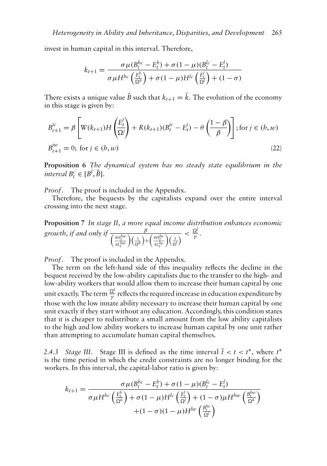
invest in human capital in this interval. Therefore,
kt+1 = σμ(Bhct − Eh
t ) + σ(1 − μ)(Blct − El
t)
σμHhc(
Eht
h
)+ σ(1 − μ)Hlc
(El
tl
)+ (1 − σ)
There exists a unique value B such that kt+1 = k. The evolution of the economyin this stage is given by:
Bjct+1 = β
[W(kt+1)H
(Ej
t
j
)+ R(kt+1)(B
jct − Ej
t) − θ
(1 − β
β
)]; for j ∈ (h, w)
Bjwt+1 = 0; for j ∈ (h, w) (22)
Proposition 6 The dynamical system has no steady state equilibrium in theinterval Bc
t ∈ [Bl, B].Proof. The proof is included in the Appendix.
Therefore, the bequests by the capitalists expand over the entire intervalcrossing into the next stage.
Proposition 7 In stage II, a more equal income distribution enhances economicgrowth, if and only if β(
∂Hhwt
∂Lhwt
)(1
h
)+(
∂Hlwt
∂Llwt
)(1l
) < l
γ.
Proof. The proof is included in the Appendix.The term on the left-hand side of this inequality reflects the decline in the
bequest received by the low-ability capitalists due to the transfer to the high- andlow-ability workers that would allow them to increase their human capital by oneunit exactly. The term l
γreflects the required increase in education expenditure by
those with the low innate ability necessary to increase their human capital by oneunit exactly if they start without any education. Accordingly, this condition statesthat it is cheaper to redistribute a small amount from the low ability capitaliststo the high and low ability workers to increase human capital by one unit ratherthan attempting to accumulate human capital themselves.
2.4.3 Stage III. Stage III is defined as the time interval t < t < t∗, where t∗is the time period in which the credit constraints are no longer binding for theworkers. In this interval, the capital-labor ratio is given by:
kt+1 = σμ(Bhct − Eh
t ) + σ(1 − μ)(Blct − El
t)
σμHhc(
Eht
h
)+ σ(1 − μ)Hlc
(El
tl
)+ (1 − σ)μHhw
(Bhw
th
)+(1 − σ)(1 − μ)Hlw
(Blw
tl
)
266 S. Khalifa
The evolution of the economy is given by:
Bjct+1 = β
[W(kt+1)H
(Ej
t
j
)+ R(kt+1)(B
jct − Ej
t) − θ
(1 − β
β
)]; for j ∈ (h, w)
Bjwt+1 = max
{β
[W(kt+1)H
(Bjw
t
j
)− θ
(1 − β
β
)], 0
}; for j ∈ (h, w) (23)
Proposition 8 The dynamical system has no steady state equilibrium in the timeinterval t < t < t∗.
Proof. The proof is included in the Appendix.In the initial period kt+1 > k, the bequests Bhw
t > 0 and Blwt > 0, and therefore
the sequence {Bct , Bw
t } increases monotonically over the time period t < t < t∗.Therefore, the economy proceeds into stage IV.
Proposition 9 In stage III, a more equal income distribution enhances economicgrowth, if and only if β(
∂Hhwt
∂Lhwt
)(1
h
)+(
∂Hlwt
∂Llwt
)(1l
) < l
γ.
Proof. The proof is included in the Appendix.
2.4.4 Stage IV. Stage IV is defined as the time interval t ≥ t∗, where creditconstraints are no longer binding. The capital-labor ratio is given by:
kt+1 =σμ(Bhc
t − Eht ) + σ(1 − μ)(Blc
t − Eht ) + (1 − σ)
×μ(Bhwt − Eh
t ) + (1 − σ)(1 − μ)(Blwt − El
t)
σμHhc(
Eht
h
)+ σ(1 − μ)Hlc
(El
tl
)+ (1 − σ)
×μHhw(
Eht
h
)+ (1 − σ)(1 − μ)Hlw
(El
tl
)
The evolution of the economy is given by:
Bjct+1 = β
[W(kt+1)H
(Ej
t
j
)+ R(kt+1)(B
jct − Ej
t) − θ
(1 − β
β
)]; for j ∈ (h, w)
Bjwt+1 = β
[W(kt+1)H
(Ej
t
j
)+ R(kt+1)(B
jwt − Ej
t) − θ
(1 − β
β
)]; for j ∈ (h, w)
(24)
Heterogeneity in Ability and Inheritance, Disparities, and Development 267
Proposition 10 In Stage IV, income redistribution has no effect on economicgrowth.
Proof. The proof is included in the Appendix.
3. Estimation
In this section, the predictions of the model are tested empirically using the thresh-old estimation technique developed in Hansen (1999). The model suggests thatthe relationship between economic growth and income inequality depends on thedevelopment stage of the economy. In the early stages, equality enhances economicgrowth, while in the later stage inequality does not have an effect on growth. Theadvantage of the threshold regression model is that it allows the level of GDP percapita to determine the existence and significance of a threshold level in the rela-tionship between income inequality and economic growth, rather than imposinga priori an arbitrary classification scheme. The econometric specification is typ-ical to that used in the literature to estimate the effect of income inequality oneconomic growth. The specification estimates the growth rate as a function oflagged income inequality, a lagged measure of human capital investment, and alagged measure of physical capital investment. The threshold estimation modelis, thus, given by:
Growthit =
⎧⎪⎪⎨⎪⎪⎩
μi + β1Giniit−1 + φ1Educationit−1
+φ2Investmentit−1 + eitif GDPit−1 ≤ GT
μi + β2Giniit−1 + φ1Educationit−1
+φ2Investmentit−1 + eitif GDPit−1 > GT
(25)
where the subscript i indexes the country, and the subscript t indexes time. Thedependent variable Growthit denotes the growth rate of GDP per capita in countryi in year t. The variable Giniit−1 is a measure of the Gini coefficient in country i inyear t − 1. The variable Educationit−1 is a measure of educational attainment incountry i in year t − 1, and is considered as a proxy for human capital investmentas is standard in the literature. The variable Investmentit−1 is the investment shareof real GDP per capita in country i in year t − 1. The variable GDPit−1 denotesreal GDP per capita in country i in year t − 1, and is the threshold variabledetermining the stage of development. It is standard in the literature to includeinitial real GDP per capita, as an independent variable, to test for convergence. Ifincluded, the equation contains a lagged endogenous variable which is the incometerm. This is apparent when the equation is rewritten with growth expressed asthe difference in the logarithm of income levels. As Hansen’s (1999) technique isdeveloped for a non-dynamic panel, lagged real GDP per capita is excluded fromthis regression.
Obviously, the threshold GDP per capita determines whether the coefficient onthe Gini coefficient is positive or negative. In this context, the observations aredivided into two regimes depending on whether the threshold variable GDPit−1is smaller or larger than the threshold GT. The regimes are distinguished by
differing regression slopes, β1 and β2. According to the predictions of the model,the coefficient β1 is expected to be negative, while the coefficient β2 is not expectedto be statistically significant. Another way of writing the equation of interest is:
where I(.) is the indicator function. A balanced panel annual data is used for 70countries that cover the period from 1971 to 1999. A Gini coefficient compiled bythe University of Texas Inequality Project is used as a proxy for income inequality.The average years of total education in the population aged over 15, from Barroand Lee data on educational attainment, is used as a measure of human capital.Finally, real GDP per capita, and the investment share of real GDP per capita areextracted from the Penn World Tables 6.2. Detailed data description is includedin the Appendix. Summary statistics of the variables used in the estimation areprovided in Table 1.
To determine the number of thresholds, the model is estimated by least squaresallowing for zero, one, two and three thresholds. The test statistics F1, F2, and F3,along with their bootstrap3 p-values are shown in column 1 in Table 2. The testfor a single threshold F1 is highly significant with a bootstrap p-value of zero, andthe test for a double threshold F2 is also significant with a bootstrap p-value of0.006667. On the other hand, the test for a triple threshold F3 is not significant,with a bootstrap p-value of 0.573333. Thus, we conclude that there is evidencethat there are two thresholds in the regression relationship. For the remainder ofthe analysis, we work with the double threshold model as follows:
Growthit = μi + β1Giniit−1I(GDPit−1 ≤ GT1)
+ β2Giniit−1I(GT1 < GDPit−1 ≤ GT2)
+ β3Giniit−1I(GT2 < GDPit−1) + φ1Educationit−1
+ φ2Investmentit−1 + eit (27)
We refer to this as regression 1. We also estimate another model, where we replacetotal educational attainment with male and female educational attainment. The
3300 bootstrap replications are used for each of the three bootstrap tests.
Heterogeneity in Ability and Inheritance, Disparities, and Development 269
Table 2. Tests for thresholds effects
Regression 1 Regression 2
Test for single thresholdF1 87.368146 87.239120P-value 0.000000 0.000000(10%, 5%, 1% critical values) (21.482757, 30.922510,
variable MaleEducationit−1 is a measure of male educational attainment in coun-try i in year t − 1, and the variable FemaleEducationit−1 is a measure of femaleeducational attainment in country i in year t − 1. The average years of educationin the male and female population aged over 15 is extracted from Barro and Leedata on educational attainment. The test statistics F1, F2, and F3, along with their
Figure 2. Confidence interval construction in double threshold model.
270 S. Khalifa
Figure 3. Confidence interval construction in double threshold model.
bootstrap4 p-values are shown in column 2 in Table 2. We can conclude that thereare also two thresholds in the regression relationship 2. Regression 2 is, thus,given by:
+ φ2FemaleEducationit−1 + φ3Investmentit−1 + eit (28)
In both regressions, the point estimates of the two thresholds are $1079.172759and $1347.094572, and their asymptotic 99% confidence intervals are[1079.172759, 1079.172759] and [1347.094572, 1380.328760], respectively. Moreinformation can be learned from plots of the concentrated likelihood ratio func-tion displayed in Figures 2 and 3. To examine the first-step likelihood ratiofunction which is computed when estimating a single threshold model, the first-step threshold estimate is the point where the likelihood function equals zero,which occurs at GT1 = 1079.172759. There is a second dip in the likelihood ratioaround the second-step estimate GT2 = 1347.094572.
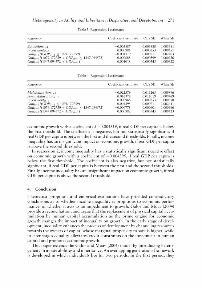
The regression slope estimates, conventional OLS standard errors, and white-correlated standard errors are reported in Table 3 for regression 1, and in Table 4for regression 2. The estimates of primary interest in regression 1 are those on theGini coefficient. Income inequality has a statistically significant negative effect on
4300 bootstrap replications are used for each of the three bootstrap tests.
Heterogeneity in Ability and Inheritance, Disparities, and Development 271
economic growth with a coefficient of −0.004319, if real GDP per capita is belowthe first threshold. The coefficient is negative, but not statistically significant, ifreal GDP per capita is between the first and the second thresholds. Finally, incomeinequality has an insignificant impact on economic growth, if real GDP per capitais above the second threshold.
In regression 2, income inequality has a statistically significant negative effecton economic growth with a coefficient of −0.004395, if real GDP per capita isbelow the first threshold. The coefficient is also negative, but not statisticallysignificant, if real GDP per capita is between the first and the second thresholds.Finally, income inequality has an insignificant impact on economic growth, if realGDP per capita is above the second threshold.
4. Conclusion
Theoretical proposals and empirical estimations have provided contradictoryconclusions as to whether income inequality is propitious to economic perfor-mance, or whether it acts as an impediment to growth. Galor and Moav (2004)provide a reconciliation, and argue that the replacement of physical capital accu-mulation by human capital accumulation as the prime engine for economicgrowth changes the impact of inequality on growth. In the early stage of devel-opment, inequality enhances the process of development by channeling resourcestowards the owners of capital whose marginal propensity to save is higher, whilein later stages equality alleviates credit constraints on the investment in humancapital and promotes economic growth.
This paper extends the Galor and Moav (2004) model by introducing hetero-geneity in innate abilities and inheritance. An overlapping generations frameworkis developed in which individuals live for two periods. In the first period, they
272 S. Khalifa
receive their inheritance and their innate abilities are revealed. Individuals decideon their optimal education level, and divide their inheritance between spendingon education and saving for the second period, and then devote their entire timeto the acquisition of human capital. In the second period, individuals supplytheir efficiency units of labor and allocate the resulting labor income along withthe return to their saving between consumption and bequests to their offsprings.Initial capital stock is owned entirely by capitalists, while the remainder of thepopulation are referred to as workers. There are only two types of innate abilities:high and low.
In this context, a more equitable distribution of income enhances economicgrowth if the economy is lower than a threshold capital-labor ratio, while incomeinequality has an insignificant effect above this threshold. The predictions ofthe model are tested empirically using the Hansen (1999) threshold estimation.The results, using a panel of 70 countries for the period 1971–1999, suggestthat there is a statistically significant threshold income per capita, below whichthe coefficient on the relationship between inequality and economic growth issignificantly negative and above which the estimate is not significant.
Acknowledgements
I thank Christopher Carroll, an anonymous referee, and participants in the Southern Economic AssociationAnnual Meeting 2007, and California State University, Fullerton, Seminar Series. Any remaining errors are myown.
References
Alesina, A. & Rodrik, D. (1994) Distributive politics and economic growth, The Quarterly Journal of Economics,109, pp. 465–490.
Altonji, J., Hayashi, F. & Kotlikoff, L. (1997) Parental altruism and inter vivos transfers: theory and evidence,Journal of Political Economy, 105, pp. 1121–1166.
Barro, R. (2000) Inequality and growth in a panel of countries, Journal of Economic Growth, 5, pp. 5–32.Barro, Robert & Lee, Jong-Wha (2000) International data on educational attainment: updates and implications.
Center for International Development Working Paper 42.Carroll, C. (2000) Why do the rich save so much, in: J. Slemrod (Ed) Does Atlas Shrug? Economic Consequences
of Taxing the Rich (London: Cambridge University Press).Deininger, K. & Squire, L. (1996) A new data set measuring income inequality, The World Bank Economic
Review, 10(3), pp. 565–591.Forbes, K. (2000) A reassessment of the relationship between inequality and growth, The American Economic
Review, 90, pp. 869–887.Galbraith, J. & Kum, H. (2004) Estimating the inequality of household incomes: a statistical approach to the
creation of a dense and consistent global dataset, University of Texas Inequality Project Working Paper 22.Galor, O. & Moav, O. (2004) From physical to human capital accumulation: inequality and the process of
development, Review of Economic Studies, 71, pp. 1001–1026.Hansen, B. (1999) Threshold effects in non-dynamic panels: estimation, testing, and inference, Journal of
Econometrics, 93, pp. 345–368.Kuznets, S. (1955) Economic growth and income inequality, The American Economic Review, 45, pp. 1–28.Perotti, R. (1992) Income distribution, politics, and growth, The American Economic Review, 82, pp. 311–316.Perotti, R. (1993) Political equilibrium, income distribution, and growth, Review of Economic Studies, 60(4),
pp. 755–776.Persson, T. & Tabellini, G. (1994) Is inequality harmful for growth? The American Economic Review, 84,
pp. 600–621.
Heterogeneity in Ability and Inheritance, Disparities, and Development 273
Appendix
Data
The estimation uses annual data that covers the period from 1971 to 1999 for 70countries, namely: Algeria, Australia, Austria, Bangladesh, Barbados, Belgium,Bolivia, Cameroon, Canada, Central Africa, Chile, Colombia, Cyprus, Den-mark, Dominican Republic, Ecuador, El Salvador, Fiji, Finland, Germany, Ghana,Greece, Guatemala, Haiti, Hong Kong, Hungary, Iceland, India, Indonesia, Iran,Iraq, Ireland, Israel, Italy, Jamaica, Japan, Jordan, Kenya, Korea, Kuwait, Malawi,Malaysia, Mauritius, Mexico, Netherlands, New Zealand, Nicaragua, Norway,Pakistan, Panama, Papua New Guinea, Philippines, Poland, Portugal, Senegal,Singapore, South Africa, Spain, Swaziland, Sweden, Syria, Taiwan, Tanzania,Tunisia, Turkey, United Kingdom, United States of America, Uruguay, Venezuela,and Zimbabwe.
The variables used in the estimations are described in details as follows.
Gini Coefficient. A detailed description of the Estimated Household IncomeInequality dataset, compiled by the University of Texas Inequality Project, is pro-vided in Galbraith and Kum (2004). This dataset combines data on the measure ofdispersion of pay across industrial categories in the manufacturing sector, drawnfrom the industrial database published annually by the United Nations IndustrialDevelopment Organization UNIDO, with the information in the Deininger andSquire (1996) data, resulting in a dataset for the Gini coefficient referred to as theEstimated Household Income Inequality EHII.
Gross Domestic Product. The data for real Gross Domestic Product per capita(Laspeyres) is extracted from the Penn World Tables 6.2, which is obtained byadding up consumption, investment, government and exports, and subtractingimports in any given year, where the components are obtained by extrapolatingthe 1996 values in international dollars from the Geary aggregation using nationalgrowth rates. The growth rate of GDP per capita is given by the difference in thenatural logarithm of the real GDP per capita in two consecutive years.
Education. The data for total education, male and female education arederived from the Barro and Lee International Data on Educational Attainmentin which they constructed estimates of educational attainment by sex for personsaged 15 and over. The values applied to several countries over five-year intervalsfor 1970, 1975, 1980, 1985, 1990, 1995 and 1999. The estimation procedure beganwith census information on school attainment for males and females where thedata came from individual governments as compiled by the UNESCO and othersources. We follow Forbes (2000) in using the average years of secondary school-ing in the male population, and the average years of secondary schooling in thefemale population as proxies for male and female education, respectively. As thedata are available only for the years 1970, 1975, 1980, 1985, 1990, 1995 and 1999,we use linear interpolation to derive the years in between.
274 S. Khalifa
Investment. The data for the investment share of real Gross Domestic Productper capita is extracted from the Penn World Tables 6.2.
Derivations
Proof of Proposition 1 As limLit→0 H′(Lit) = γ , then the first order conditionfor those with innate ability j satisfies H′(Lit) = R(kj)
W(kj)j = γ . Therefore, from
the first order conditions of the firm Aα(kj)α−1
A(1−α)(kj)αj = γ , which can be rearranged
as kj = j α(1−α)γ
.If kt+1 ≤ kj, then individual i of generation t with innate ability j does not
invest in education Eit = 0, and saves only if he receives a positive bequest from hisparents Bit > 0, since Sit = Bit − Eit. On the other hand, if kt+1 > kj, individuali of generation t with innate ability j invests in education where the optimal levelis given by Ej
t. However, if they do not receive any bequest from their parents,they are credit constrained since they cannot borrow to cover the expenditure oneducation, and thus they do not spend on education Eit = 0 and save nothingSit = 0. If they receive a positive bequest from their parents Bit > 0, and thisamount is lower than the optimal level Ej
t, then their expenditure on education isconstrained by this amount and they do not save as well. They can only achievethe optimal level of education if the bequest they receive from their parents isequal to or larger than the optimal amount. If larger, they save the differenceSit = Bit − Ej
t.
Proof of Proposition 2 Let k be the critical level of the capital-labor ratiobelow which individuals who do not receive bequests from their parent do notleave bequests to their offspring. That is W(k) = θ(1−β)
β. From the first-order
conditions of the firm, k =[
θ(1−β)β
A(1−α)
] 1α
, where if kt+1 ≤ k then W(kt+1) ≤θ(1−β)
β, whereas if kt+1 > k, then W(kt+1) >
θ(1−β)β
. Accordingly, Bit+1 = 0 if
kt+1 ≤ k, and Bit+1 > 0 if kt+1 > k.Assume also that once wages increase sufficiently such that workers leave
bequests to their offspring, or if kt+1 > k, investment in human capital is prof-itable for all types of workers, or kt+1 > kl. That is kl ≤ k. Since ∂ k
∂(θ(1−β)
β)
> 0, it
follows that for any given γ , there exists θ(1−β)β
sufficiently large such that kl ≤ k.
Let tl + 1 be the first period in which the capital-labor ratio exceeds kl. Thatis, since k0 < kl, it follows that kt+1 ≤ kl for all 0 ≤ t < tl. Let t + 1 be thefirst period in which the capital-labor ratio exceeds k. That is kt+1 ≤ k for all0 ≤ t < t. Then, it follows from kl ≤ k that tl ≤ t.
Heterogeneity in Ability and Inheritance, Disparities, and Development 275
Since k0 < kl, then the bequest of a worker Bw0 = 0. Furthermore, for 1 ≤ t < t,
as long as Bwt−1 = 0, the descendants do not invest in human capital, Hw
t = 1, andtherefore Bw
t = max[β(W(kt+1) − θ(1−β)β
), 0] = 0.
Proof of Proposition 3 There exists a B such that Bct+1 = 0 for Bc
t ≤ B, whereBc
t = μBhct + (1 − μ)Blc
t . Thus, B is defined, such that:
0 = β
[W(σB) + R(σB)B − θ
1 − β
β
]
0 = β
{(1 − α)A[σB]α + αA[σB]α−1B − θ
(1 − β
β
)}
Solving for B yields B = [ (θ1−ββ
)
(1−α)Aσα+αAσα−1 ]1α . Since this expression is decreasing
in A, and we assumed the technology is sufficiently productive, then Bct+1 = 0 for
Bct ≤ B as shown in Figure 1. Furthermore, Bc
t+1 is increasing and strictly concave
in the interval Bct ∈ (B, Bl], where Bl = (kl
σ) = α
(1−α)γ σl, which is independent
of A. As depicted in Figure 1, the function Bct+1 is equal to zero for Bc
t ≤ B, andit is increasing and concave for B < Bc
t ≤ Bl, and it crosses the 45◦ line once inthis interval. It is worth mentioning that in this interval, there is also Bh = (kh
σ) =
α(1−α)γ σ
h < Bl, as h < l. Hence, the dynamical system has two steady state
equilibria in the interval Bct ∈ [0, Bl]; a locally stable steady state, B0 = 0, and an
unstable steady state B. If Bct < B, the bequests contract over time and the system
converges to the steady state B0. If Bct >
�
B, the bequests expand over the entireinterval crossing into stage II. To ensure that the process of development starts instage I and ultimately takes off to stage II, it is assumed that Bc
0 ∈ (B, Bl).
Proof of Proposition 4 In stage I, if kt+1 ∈ [k0, kh], we know that Bhct > 0, and
Blct > 0, while from Proposition 2, Bhw
t = Blwt = 0. From Proposition 1, high
ability capitalists do not invest in education, so Ehct = 0, and thus Shc
t = Bhct .
Similarly, low ability capitalists do not invest in education, so Elct = 0, and
thus Slct = Blc
t . From Proposition 1, high ability workers do not invest in edu-cation, therefore Ehw
t = 0 and Shwt = 0. Similarly, low-ability workers do not
invest in education, therefore Elwt = 0 and Slw
t = 0. In this context, the aggregatephysical capital is given by Kt+1 = σμBhc
t + σ(1 − μ)Blct , while the aggregate
human capital is given by Ht+1 = 1. Therefore, output in period t + 1 is given byYt+1 = A[σμBhc
t + σ(1 − μ)Blct ]α. In this context, we have:
Bjct = β
(Wt + RtB
jct−1 − θ(1 − β)
β
)= β
(Ijct − θ(1 − β)
β
); for j ∈ (h, l)
276 S. Khalifa
If εt, that is sufficiently small, is subtracted from the period t income of thecapitalists, such that Ihc
t = Ihct − μεt and Ilc
t = Ilct − (1 − μ)εt, and redistributed
to workers such that Ihwt = Ihw
t + μεt and Ilwt = Ilw
t + (1 − μ)εt. Then, we can see
that ∂Bhct
∂εt< 0 and ∂Blc
t∂εt
< 0. In addition, as long as Ihwt <
θ(1−β)β
and Ilwt <
θ(1−β)β
,
then ∂Bhwt
∂εt= 0 and ∂Blw
t∂εt
= 0. Accordingly, the effect of redistribution on outputin period t + 1 is given by:
∂Yt+1
∂εt= ∂Yt+1
∂Kt+1
∂Kt+1
∂Bhct
∂Bhct
∂εt+ ∂Yt+1
∂Kt+1
∂Kt+1
∂Blct
∂Blct
∂εt< 0
To show that Yt+1 = Y(Yt), we have:
Yt+1 = A{σμ[βWt + βRtBhct−1 − θ(1 − β)]
+ σ(1 − μ)[βWt + βRtBlct−1 − θ(1 − β)]}α
= A{σβWt − σθ(1 − β) + βRt[σμBhct−1 + σ(1 − μ)Blc
t−1]}α
= A
⎧⎨⎩σβWt − σθ(1 − β) + βRt
⎡⎣(Yt
A
) 1α
⎤⎦⎫⎬⎭
α
Therefore, ∂Yt+1∂Yt
> 0, and thus ∂Yt+2∂Yt+1
> 0 and generally ∂Yt+n∂Yt+n−1
> 0. Therefore,redistribution at this stage of development does not enhance economic growth.
Proof of Proposition 5 In stage I, if kt+1 ∈ (kh, kl], we know that Bhct > 0, and
Blct > 0, while from Proposition 2, Bhw
t = Blwt = 0. From Proposition 1, high-
ability capitalists invest in human capital, Ehct = Bhc
t < Eht , and thus Shc
t = 0. FromProposition 1, low-ability capitalists do not invest in education, so Elc
t = 0, andthus Slc
t = Blct . From Proposition 1, high-ability workers are credit constrained, so
they cannot invest in education, Ehwt = 0, and thus Shw
t = 0. From Proposition 1,low-ability workers do not invest in education Elw
t = 0, thus Slwt = 0. In this
context, aggregate physical capital is given byKt+1 = σ(1 − μ)Blct . On the other
hand, aggregate human capital is given by Ht+1 = σμHhc(Bhc
th ) + σ(1 − μ) +
(1 − σ). Therefore, output in period t + 1 is given by:
Yt+1 = A
[σμHhc
(Bhc
t
h
)+ σ(1 − μ) + (1 − σ)
]1−α
[σ(1 − μ)Blct ]α
In this context, we have:
Blct = β
(Wt + RtBlc
t−1 − θ(1 − β)
β
)= β
(Ilct − θ(1 − β)
β
)
If an amount εt, that is sufficiently small, is subtracted from the period t incomeof low-ability capitalists and transferred to the high ability workers, such that
Heterogeneity in Ability and Inheritance, Disparities, and Development 277
Ilct = Ilc
t − σ(1 − μ)εt. Then, the aggregate human capital, after redistribution,is given by:
Ht+1 = σμHhc
(Bhc
t
h
)+ σ(1 − μ) + (1 − σ)μHhw
⎛⎝[
σ(1−μ)(1−σ)μ
εt
]h
⎞⎠
+ (1 − σ)(1 − μ)
Then ∂ Ilct
∂εt< 0, and accordingly ∂Blc
t∂εt
= −β < 0. Similarly, as εt is redistributed tothe high-ability workers to finance their education and taking into consideration
the properties of the human capital function, then ∂Hhwt
∂εt> 0. The final effect on
output in period t + 1 of the redistribution is given by:
∂Yt+1
∂εt= ∂Yt+1
∂Ht+1
∂Ht+1
∂Hhwt
∂Hhwt
∂Lhwt
∂Lhwt
∂εt+ ∂Yt+1
∂Kt+1
∂Kt+1
∂Blct
∂Blct
∂εt
= A(1 − α)H−αt+1Kα
t+1(1 − σ)μ∂Hhw
t
∂Lhwt
[σ(1−μ)(1−σ)μ
]h
− AH1−αt+1 αKα−1
t+1 σ(1 − μ)β
Therefore, ∂Yt+1∂εt
> 0 if and only if:
A(1 − α)H−αt+1Kα
t+1(1 − σ)μ∂Hhw
t
∂Lhwt
[σ(1−μ)(1−σ)μ
]h
> AH1−αt+1 αKα−1
t+1 σ(1 − μ)β
This is satisfied if:
(1 − α)kαt+1
∂Hhwt
∂Lhwt
> hαkα−1t+1 β
This can be arranged as:
kt+1 >α
1 − α
βh
(∂Hhw
t∂Lhw
t)
As we are focusing on kh < kt+1 ≤ kl, or α1−α
h
γ< kt+1 ≤ α
1−αl
γ. Then, there
exists a situation where redistribution from low-ability capitalists to high-ability
workers induces growth, ∂Yt+1∂εt
> 0, if an only if βh
(∂Hhw
t∂Lhw
t)
< l
γ.
Proof of Proposition 6 For any given B > Bl, where Bl is independent of A,since β[W(B) + R(B)B − θ
1−ββ
] is strictly increasing in A, there exists a suffi-
ciently large A such that β[W(B) + R(B)B − θ1−ββ
] > B. Note that B decreases
278 S. Khalifa
with A, however a sufficiently large θ1−ββ
ensures that k > kl. Assume that
β[W(B) + R(B)B − θ1−ββ
] > B. This implies, in the absence of investment inhuman capital that:
β[W(Bct ) + R(Bc
t )Bct − θ
1 − β
β] > Bc
t ; for Bct ∈ [Bl, B]
Since∂Bc
t+1∂Ec
t> 0 for Bc
t ∈ [Bl, B], and Ejct ∈ [0, Ej
t], then Bct+1 ≥ β[W(Bc
t ) +R(Bc
t )Bct − θ
1−ββ
] > Bct ; for Bc
t ∈ [Bl, B]. Therefore, the dynamical system has nosteady state equilibrium in this interval.
Proof of Proposition 7 In stage II, we know that Bhct > 0, and Blc
t > 0, whilefrom Proposition 2, Bhw
t = Blwt = 0. From Proposition 1, high ability capitalists
invest in human capital, Ehct = Eh
t , and thus Shct = (Bhc
t − Eht ). From Proposition 1,
low ability capitalists invest in education, so Elct = El
t, and thus Slct = (Blc
t − Elt).
From Proposition 1, high-ability workers are credit constrained, so they cannot invest in education, Ehw
t = 0, and thus Shwt = 0. From Proposition 1, low-
ability workers do not invest in education Elwt = 0, thus Slw
t = 0. In this context,aggregate physical capital is given by:
Kt+1 = σμ(Bhct − Eh
t ) + σ(1 − μ)(Blct − El
t)
On the other hand, aggregate human capital is given by:
Ht+1 = σμHhc
(Eh
t
h
)+ σ(1 − μ)Hlc
(El
t
l
)+ (1 − σ)
Therefore, output in period t + 1 is given by:
Yt+1 = A
[σμHhc
(Eh
t
h
)+ σ(1 − μ)Hlc
(El
t
l
)+ (1 − σ)
]1−α
× [σμ(Bhct − Eh
t ) + σ(1 − μ)(Blct − El
t)]α
If an amount εt, that is sufficiently small, is subtracted from the period t income ofcapitalists and transferred to the workers, where Bhc
t − Eht > εt, and Blc
t − Elt > εt,
then we have Ihct = Ihc
t − μεt and Ilct = Ilc
t − (1 − μ)εt, such that Ihwt = Ihw
t + μεt
and Ilwt = I1w
t + (1 − μ)εt. After redistribution, the aggregate human capital is
Heterogeneity in Ability and Inheritance, Disparities, and Development 279
given by:
Ht+1 = σμHhc
(Eh
t
h
)+ σ(1 − μ)Hlc
(El
t
l
)+ (1 − σ)μHhw
⎛⎝[
σ(1−σ)μ
]εt
h
⎞⎠
+ (1 − σ)(1 − μ)Hlw
⎛⎝[
σ(1−σ)(1−μ)
]εt
l
⎞⎠
The final effect on output in period t + 1 of the redistribution is given by:
∂Yt+1
∂εt= ∂Yt+1
∂Ht+1
∂Ht+1
∂Hhwt
∂Hhwt
∂Lhwt
∂Lhwt
∂εt+ ∂Yt+1
∂Ht+1
∂Ht+1
∂Hlwt
∂Hlwt
∂Llwt
∂Llwt
∂εt
+ ∂Yt+1
∂Kt+1
∂Kt+1
∂Bhct
∂Bhct
∂εt+ ∂Yt+1
∂Kt+1
∂Kt+1
∂Blct
∂Blct
∂εt
= A(1 − α)H−αt+1Kα
t+1(1 − σ)μ∂Hhw
t
∂Lhwt
[σ
(1−σ)μ
]h
+ A(1 − α)H−αt+1Kα
t+1(1 − σ)(1 − μ)∂Hlw
t
∂Llwt
[σ
(1−σ)(1−μ)
]l
− AH1−αt+1 αKα−1
t+1 σμβ − AH1−αt+1 αKα−1
t+1 σ(1 − μ)β
Therefore ∂Yt+1∂εt
> 0 if and only if:
A(1 − α)H−αt+1Kα
t+1(1 − σ)μ∂Hhw
t
∂Lhwt
[ σ(1−σ)μ
]h
+ A(1 − α)H−αt+1Kα
t+1(1 − σ)(1 − μ)∂Hlw
t
∂Llwt
[ σ(1−σ)(1−μ)
]l
> AH1−αt+1 αKα−1
t+1 σμβ + AH1−αt+1 αKα−1
t+1 σ(1 − μ)β
This is satisfied if:
(1 − α)kαt+1
[∂Hhw
t
∂Lhwt
σ
h+ ∂Hlw
t
∂Llwt
σ
l
]> αkα−1
t+1 σβ
which can be rearranged as:
kt+1 >αβ
(1 − α)[
∂Hhwt
∂Lhwt
1h + ∂Hlw
t∂Llw
t
1l
]
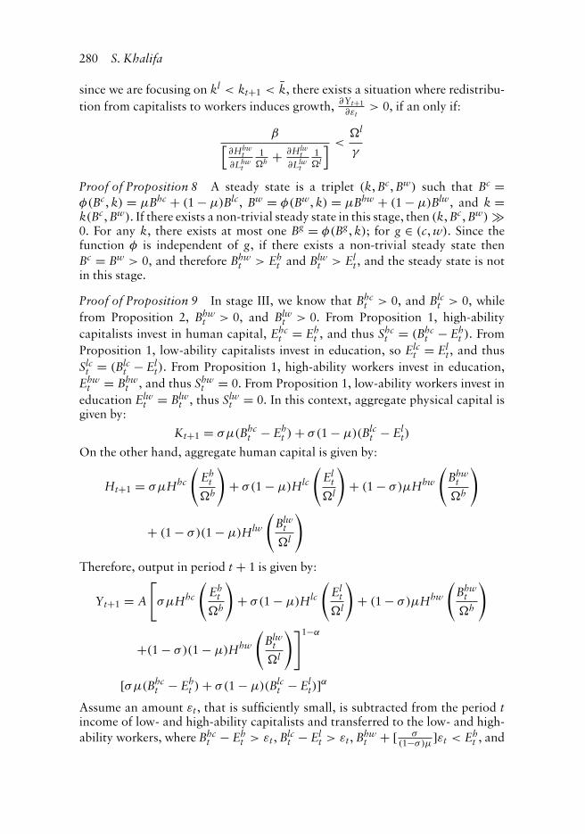
280 S. Khalifa
since we are focusing on kl < kt+1 < k, there exists a situation where redistribu-tion from capitalists to workers induces growth, ∂Yt+1
∂εt> 0, if an only if:
β[∂Hhw
t∂Lhw
t
1h + ∂Hlw
t∂Llw
t
1l
] <l
γ
Proof of Proposition 8 A steady state is a triplet (k, Bc, Bw) such that Bc =φ(Bc, k) = μBhc + (1 − μ)Blc, Bw = φ(Bw, k) = μBhw + (1 − μ)Blw, and k =k(Bc, Bw). If there exists a non-trivial steady state in this stage, then (k, Bc, Bw) �0. For any k, there exists at most one Bg = φ(Bg, k); for g ∈ (c, w). Since thefunction φ is independent of g, if there exists a non-trivial steady state thenBc = Bw > 0, and therefore Bhw
t > Eht and Blw
t > Elt, and the steady state is not
in this stage.
Proof of Proposition 9 In stage III, we know that Bhct > 0, and Blc
t > 0, whilefrom Proposition 2, Bhw
t > 0, and Blwt > 0. From Proposition 1, high-ability
capitalists invest in human capital, Ehct = Eh
t , and thus Shct = (Bhc
t − Eht ). From
Proposition 1, low-ability capitalists invest in education, so Elct = El
t, and thusSlc
t = (Blct − El
t). From Proposition 1, high-ability workers invest in education,Ehw
t = Bhwt , and thus Shw
t = 0. From Proposition 1, low-ability workers invest ineducation Elw
t = Blwt , thus Slw
t = 0. In this context, aggregate physical capital isgiven by:
Kt+1 = σμ(Bhct − Eh
t ) + σ(1 − μ)(Blct − El
t)
On the other hand, aggregate human capital is given by:
Ht+1 = σμHhc
(Eh
t
h
)+ σ(1 − μ)Hlc
(El
t
l
)+ (1 − σ)μHhw
(Bhw
t
h
)
+ (1 − σ)(1 − μ)Hlw
(Blw
t
l
)
Therefore, output in period t + 1 is given by:
Yt+1 = A
[σμHhc
(Eh
t
h
)+ σ(1 − μ)Hlc
(El
t
l
)+ (1 − σ)μHhw
(Bhw
t
h
)
+(1 − σ)(1 − μ)Hhw
(Blw
t
l
)]1−α
[σμ(Bhct − Eh
t ) + σ(1 − μ)(Blct − El
t)]αAssume an amount εt, that is sufficiently small, is subtracted from the period tincome of low- and high-ability capitalists and transferred to the low- and high-ability workers, where Bhc
t − Eht > εt, Blc
t − Elt > εt, Bhw
t + [ σ(1−σ)μ
]εt < Eht , and
Heterogeneity in Ability and Inheritance, Disparities, and Development 281
Blwt + [ σ
(1−σ)(1−μ)]εt < El
t. After redistribution, the aggregate human capital isgiven by:
Ht+1 = σμHhc
(Eh
t
h
)+ σ(1 − μ)Hlc
(El
t
l
)
+ (1 − σ)μHhw
⎛⎝Bhw
t +[
σ(1−σ)μ
]εt
h
⎞⎠
+ (1 − σ)(1 − μ)Hlw
⎛⎝Blw
t +[
σ(1−σ)(1−μ)
]εt
l
⎞⎠
The final effect on output in period t + 1 of the redistribution is given by:
∂Yt+1
∂εt= ∂Yt+1
∂Ht+1
∂Ht+1
∂Hhwt
∂Hhwt
∂Lhwt
∂Lhwt
∂εt+ ∂Yt+1
∂Ht+1
∂Ht+1
∂Hlwt
∂Hlwt
∂Llwt
∂Llwt
∂εt
+ ∂Yt+1
∂Kt+1
∂Kt+1
∂Bhct
∂Bhct
∂εt+ ∂Yt+1
∂Kt+1
∂Kt+1
∂Bhct
∂Bhct
∂εt
= A(1 − α)H−αt+1Kα
t+1(1 − σ)μ∂Hhw
t
∂Lhwt
[σ
(1−σ)μ
]h
+ A (1 − α) H−αt+1Kα
t+1(1 − σ)(1 − μ)∂Hlw
t
∂Llwt
[σ
(1−σ)(1−μ)
]l
− AH1−αt+1 αKα−1
t+1 σμβ − AH1−αt+1 αKα−1
t+1 σ(1 − μ)β
Therefore, ∂Yt+1∂εt
> 0 if and only if:
(1 − α)kαt+1
[∂Hhw
t
∂Lhwt
σ
h+ ∂Hlw
t
∂Llwt
σ
l
]> αkα−1
t+1 σβ
which is the same condition as in Proposition 7.
Proof of Proposition 10 In stage IV, we know that Bhct > 0, and Blc
t > 0, andfrom Proposition 2, Bhw
t > 0, and Blwt > 0. From Proposition 1, high-ability
capitalists invest in human capital, Ehct = Eh
t , and thus Shct = (Bhc
t − Eht ). From
Proposition 1, low-ability capitalists invest in education, so Elct = El
t, and thusSlc
t = (Blct − El
t). From Proposition 1, high-ability workers invest in education,Ehw
t = Eht , and thus Shw
t = (Bhwt − Eh
t ). From Proposition 1, low-ability workers
282 S. Khalifa
invest in education Elwt = El
t, thus Slwt = (Blw
t − Elt). In this context, aggregate
physical capital is given by:
Kt+1 = σμ(
Bhct − Eh
t
)+ σ(1 − μ)
(Blc
t − Elt
)+ (1 − σ)μ
(Bhw
t − Eht
)+ (1 − σ)(1 − μ)
(Blw
t − Elt
)On the other hand, aggregate human capital is given by:
Ht+1 = σμHhc
(Eh
t
h
)+ σ(1 − μ)Hlc
(El
t
l
)+ (1 − σ)μHhw
(Eh
t
h
)
+ (1 − σ)(1 − μ)Hlw
(El
t
l
)
Therefore, output in period t + 1 is given by:
Yt+1 = A
[σμHhc
(Eh
t
h
)+ σ(1 − μ)Hlc
(El
t
l
)+ (1 − σ)μHhw
(Eh
t
h
)
+(1 − σ)(1 − μ)Hlw
(El
t
l
)]1−α
[σμ(Bhc
t − Eht ) + σ(1 − μ)(Blc
t − Elt) + (1 − σ)μ(Bhw
t − Eht )
+(1 − σ)(1 − μ)(Blwt − El
t)]α
Assume an amount εt, that is sufficiently small, is subtracted from the period tincome of the low- and high-ability capitalists and transferred to the low- andhigh-ability workers, where Bhc
t − Eht > εt, and Blc
t − Elt > εt. After redistribu-
tion, the aggregate human capital remains the same as before the redistribution,since all types are already investing the optimal amount of expenditure oneducation. Therefore, ∂Yt+1/∂εt = 0.