Heterogeneity in the Gender Wage Gap in

Canada

Luiza Antonie

University of Guelph lantonie@uoguelph.ca

Miana Plesca University of Guelph miplesca@uoguelph.ca

Jennifer Teng Independent Researcher jiayuanteng@gmail.com

Department of Economics and Finance

University of Guelph

Discussion Paper 2016-03

Heterogeneity in the Gender Wage Gap in Canada

Luiza Antonie, University of Guelph∗

Miana Plesca, University of GuelphJennifer Teng, Independent Researcher

April 15, 2016

JEL Codes: J31, J16, J38Keywords: Gender wage gap, Pay equity

Abstract

There is significant heterogeneity in the male-female wage gap depending on individuals’education, income, and labour supply choices. Using data from the Canadian Census and fromthe Labour Force Survey, we document to what extent the gap in hourly wages gets compoundedby a gender gap in hours worked, making the annual gender pay gap much larger. Within full-time full-year, full-time part year, and part-time jobs, we find much smaller gaps than the overallone, even conditional on detailed occupations. This suggests a different selection by gender intofull-time and part-time jobs, with women of higher earnings potential selecting into part-timework. We document that men are more likely to be promoted than women, regardless of maritalstatus, while women are more likely to select into part-time jobs or be absent from work if theyhave children in their care. Furthermore, the wage gap is very small for younger people andit increases with age, even for single individuals, providing suggestive evidence for statisticaldiscrimination. The male-female wage gap decreases with education, at all quantiles of theincome distribution, except for a glass ceiling effect observable for the top 10% of the universitywage distribution. We look more deeply at this glass ceiling effect by assigning gender to theindividuals on Ontario’s Sunshine list of public salary disclosure for top earners. We documenta gender imbalance on the list, with twice more men than women making the list, but nosubstantive gender wage gap. Given all these findings, we contend that wage equality in thelabour market can only be achieved in conjunction with gender equality in the household, andthat effective policies to target the remaining wage gap should address labour supply and childrearing channels.

∗We gratefully acknowledge the support from the Ontario Pay Equity Commission grant. We thank AndrewDAngelo for assistance with the Sunshine List data, Scott Strickland for assistance with the literature survey, andEsmond Lun for research assistance. Gary Grewal and Kris Inwood have provided valuable comments, for which weare grateful.

1

List of Tables

1 Evolution of the Gender Pay Gap, Census 1996-2011, all jobs . . . . . . . . . . . . . 232 Evolution of the Gender Pay Gap, Census 1996-2011, FTFY . . . . . . . . . . . . . . 243 Evolution of the Gender Pay Gap, Census 1996-2011, FT Part Year . . . . . . . . . 254 Evolution of the Gender Pay Gap, Census 1996-2011, Part Time . . . . . . . . . . . 265 Evolution of the Gender Pay Gap, Public LFS, Hourly Wages . . . . . . . . . . . . . 276 Oaxaca-Blinder Wage Gap Decomposition, LFS (RDC access) 1997-2013 . . . . . . . 297 Heterogeneity in the wage gap by marital status and age groups, controlling by

education and job type. Public LFS, 1997 to 2014 . . . . . . . . . . . . . . . . . . . 308 Relative Gender Wage Gap, Census . . . . . . . . . . . . . . . . . . . . . . . . . . . 319 Probability of promotion by gender . . . . . . . . . . . . . . . . . . . . . . . . . . . . 3310 Probability of Working Part-time and Probability of Leaving Job Due to Children

and Family Obligations. Source: 2013 public LFS . . . . . . . . . . . . . . . . . . . . 3411 Probability of Being Employed Absent from Work . . . . . . . . . . . . . . . . . . . 3512 Number of Records on Sunshine List (Nominal and Real Thresholds) . . . . . . . . . 3613 Number of Records on Sunshine List by Sector (Nominal and Real Thresholds) . . . 3714 Percent women across time and (aggregated) sectors . . . . . . . . . . . . . . . . . . 38

List of Figures

1 Evolution of the Gender Wage Gap, Canada (Census). . . . . . . . . . . . . . . . . . 392 Gender Wage Gap Across the Income Distribution, Census Annual Earnings. . . . . 403 Gender Wage Gap Across the Income Distribution, Census (imputed) Hourly Earnings. 414 Wage Gap by Public/Private Sectors, LFS. . . . . . . . . . . . . . . . . . . . . . . . 425 Wage Gap by Education and Public/Private Sectors, LFS. . . . . . . . . . . . . . . . 436 Number of Records in the Sunshine List (nominal $ and real $ thresholds). . . . . . 437 Evolution of the Gender Ratio in the Sunshine List (nominal $ and real $ thresholds). 448 Pay Gap between Men and Women in the Sunshine List. . . . . . . . . . . . . . . . . 459 Gender Gap at Quantiles of Earnings Distribution, Sunshine List. . . . . . . . . . . . 4610 Gender Gap at Quantiles of Earnings Distribution by Sectors, Sunshine List. . . . . 47

2

1 Introduction

“It’s 2015. Probably time for wage parity.”

After last year Sony hack leaked emails revealing that female stars of the Oscar-nominatedAmerican Hustle were paid less than their male counterparts, the issue has been a hot subject inHollywood; Best Supporting Actress winner Patricia Arquette (Boyhood) concluded her acceptancespeech by declaring: “It’s our time to have wage equality once and for all, and equal rights for womenin the United States of America.” 1 Canada’s newly elected Prime-Minister Justin Trudeau hasappointed Canada’s first gender-balanced cabinet. “Because it’s 2015”, Trudeau has famously saidwhen asked why gender parity was important.2

The question of the male-female wage gap has persisted both in academic circles and in thepublic sphere. The society has evolved considerably in terms of the career expectations of women.Current university enrollment statistics show that female students make up about two thirds of thestudent body; labour force participation rates of women and the number of hours worked have beenconstantly edging closer to men’s, especially at higher levels of education. Despite this, a genderwage gap still persists. The overarching question is: what can policy do to reduce or eliminate thisgap? For policy to be effective, we must first understand where the gender wage gap is comingfrom.

This paper reviews some of the explanations provided in the literature for the gender wage gap,and provides recent estimates of the gap and relates the current gap to its evolution across time.A major contribution of this paper is its focus on the heterogeneity in the gender wage gap and itsimplications for policy, something that the literature has pad insufficient attention to. We provideevidence from the two major Canadian surveys, the Census and the Labour Force survey

First, we distinguish between hourly wage gap and annual income gap. Despite constant progressin participation and hours worked, women still work fewer hours than men do, on average. Even ifhourly wages were the same between men and women which they are not men would have a higherannual income because they work longer hours. Our research documents the difference betweenhourly and annual gender wage gaps resulting from the added gender gap in hours worked.

Second, when we restrict the analysis to similar types of jobs in terms of full-time full-yearversus part-time, the pay gap is smaller within each category than the overall gender pay gap.That is, the gap is lower within full-time full-year jobs, it is lower within full-time part-year jobs,and there is no gender wage gap within part-time jobs. This suggests a differential selection bygender into full-time jobs and part-time jobs, with women with high earnings potential choosingpart-time jobs. Moreover, men are more likely to be promoted than women, regardless of maritalstatus, and women are more likely to select into part-time jobs or be absent from work if they havechildren in their care. As suggestive evidence for statistical discrimination, where all women onaverage are expected to conform to average fertility and child rearing choices, we document thatthe gender wage gap is very small for young people, and not even present for young unmarriedindividuals, while it is increasing with age, even for singles.

Third, we document the heterogeneity in the gender wage gap across education and wagedistribution, even conditional on very refined occupation categories. The male-female wage gapdecreases with education, at all quantiles of the income distribution, except for the glass ceilingeffect observable for the top 10% of the university-educated workers. At low-skill low-educationlevels, the male-female wage gap may be generated by the difference in working conditions between

1From The Globe and Mail, February 23, 2015, Coverage of the Oscar awards ceremony by Simon Houpt.2Canadian Press, November 4 2015, Jennifer Ditchburn.

3

“tough” male jobs in mining and forestry and “soft” female jobs in retail. At high-skill high-education levels we do find evidence of a “glass-ceiling” effect, with fewer women than men beingemployed at top jobs in their organizations.

To further examine the glass ceiling, we investigate the gender wage gap for workers in theOntario public sector. Starting from 1996, all workers in Ontario establishments receiving publicsubsidies - such as local and provincial governments, crown corporations, utilities, schools, uni-versities, hospitals - have their income made public if they earn more than $100,000/year.3 Byassigning gender to individuals on Ontario’s Sunshine list, we document a gender imbalance on thelist: twice more men than women are on the Sunshine list. Nevertheless, conditional on being onthe list, we find no substantive gender wage gap, with women making form 95% to 99% of whatmen earn, depending on year and sector. The two sectors on the Sunshine List where a genderwage gap is present are Hospital and Universities/Colleges. In the Hospital sector this could bedue to a selection by gender into different types of jobs (nurses for women and surgeons for men),while in the post-secondary sector the men may be more likely to have more advanced careers.

Given these findings, we contend that effective and efficient policies to target the remainingwage gap would have to address labour supply and child rearing channels. We further contend thatfull gender wage equality in the labour market can only be achieved in conjunction with genderequality in the household. Increasing educational achievement may provide a two-fold solution:women will have an incentive to capitalize more on their increased human capital and earningpotential; moreover, technological progress may reduce the degree of “toughness” in jobs which canbecome available to women,decreasing the wage gap at lower quantiles of the income distribution.as well as encourage workers to take higher-skill higher-pay type of jobs. For women to breakthrough the glass ceiling and to encourage female participation in top jobs, policy can achieve alot. We already invest in educating women, and policy should make it easier for women to stayin the workforce or return soon after fertility interruptions, so that their human capital does notdepreciate. Potential means through which this can be achieved is by encouraging men to partakeof parental leaves as much as women do (“daddy” leaves), making sure high-quality affordablechildcare is the norm here Ontario’s all day kindergarten is an excellent example - as well asensuring a proper work-life balance in Ontario establishments.

2 Literature

2.1 Characteristics of Wage and Annual Earnings Ratio

The literature documenting the gender wage gap and its determinants is extensive. We summa-rize here some of it. Baker and Drolet (2010) found that on average the number of hours workedper week for women working full time was 3-4 hours less than men working full time. The authorsfound that this difference explained a significant amount of the annual earnings gap; specifically in2006 the female-male annual earnings ratio for full year workers aged 25-54 was 0.72 but the wageratio was 0.85. The authors also found that the wage ratio was much higher for younger work-ers, single persons and university graduates. Secondly, the academic literature shows that womenare both more likely to combine periods of paid work with periods of labour force withdrawal forfamily reasons (Drolet 2002a), and more likely to work non-standard employment jobs such aspart time or temporary jobs (Zeytinoglu and Cooke 2008). Zeytinoglu and Cooke also found thatfemale workers employed in these precarious jobs are less likely to be promoted than regular full

3Originally designed as a mechanism to “shame the fat cats” in the pubic sector, the list seems to have had theopposite effect, with public sector unions using the list when bargaining for wage increases for their membership.

4

time workers, but the same cannot be said of the male labour force. This is compounded by thefact that women tend to be disproportionately employed in low-wage occupations and low wageestablishments and industries (Drolet 2002a, 2002b; Reilly and Wirjanto 1999). Hence while someproportion of the pay gap may be accounted for by differences in the choice of hours worked, typeof employment, occupation or industry, the proportion that is not explained by this may be due tobaseless discrimination against women by employers. Finally, it is also necessary to consider thatthere is evidence of a glass ceiling effect in Canada where a large male-female pay gap exists atthe high end of the pay distribution (Baker et al. 1995; Yap and Konrad 2009). In fact, Cannings(1998a) showed that female managers are 80% as likely to be promoted as males.

2.2 Changes in Wage and Earnings Gap Over Time

Documenting how the male-female gap in pay has changed over time, Baker and Drolet (2010)found that women have significantly increased their levels of educational achievement and labourmarket participation since the 1970s. The authors also found that the wage ratio had increasedover the past fifteen years while the earnings ratio has not moved. Drolet (2011) found that theincrease in the wage ratio has been due to higher growth in women’s relative wages compared tomen. The author found that this has been driven by a “cohort effect” such that men and womenentering today’s labour market are more alike in terms of characteristics like education and wagesthan in the past and their wages are less likely to diverge over time than in the past which hasresulted in the convergence of hourly wages. However, Baker and Drolet (2010) also find that, whencontrolling for gender differences in productive characteristics, females have increasingly higherlevels than males. Hence, the authors argue that if females received the same returns to productivecharacteristics then they would receive higher wages than men. Thus as the wage gap has fallen overtime the proportion of the gap that is not explained by differences in productive characteristics,specifically the returns to productive characteristics, has grown to near 100%. Finally, there isalso evidence that women with conventionally unobserved traits that yield a wage premium, whichare not analysed by Baker and Drolet (2010), have been increasingly drawn into the higher end ofthe labour market which could indicate rising returns to skill (Blau and Kahn 2006; Mulligan andRubenstein 2008; Weinberger and Kuhn 2010; Black and Spitz-Oener 2010).

2.3 Explanations for Gender Gap

2.3.1 Job Experience and Occupational Choice

As identified above, while women in Canada have increased their levels of productive charac-teristics there is evidence that a significant proportion of the gender pay gap is explained by joband occupation choice within the labour market. Drolet (2002a, 2002b) found that controlling forlabour market experience explained a portion of the pay gap. In addition, a number of studies havepointed to the importance of men and women working in different occupations as an explanation forthe gender pay gap (Fortin and Huberman (2002), Drolet (2002a), Boudarbar and Connolly (2013).However, the extent to which occupation choice effects the gender gap varies at different pointsalong the wage distribution. Examining the gender wage gap for workers with post-secondary ed-ucation, Boudarbat and Connolly (2013) found that occupational dummies explain 37% of the gapat the mean, 112% at the 10th percentile of the wage distribution, and 17.7% at the 90th percentile.The ability of occupational choice as an explanation for the gender pay gap has also been shown toincrease with the use of occupation-specific skills rather than occupation dummy variables. Specifi-cally, Baker and Fortin (2001), looking at data from 1987 and 1988, found men are paid significantlyless in female dominated occupations than in mixed or male dominated occupations but there is

5

no substantial penalty to women who work in male-dominated or mixed occupations. In addition,Teng (2015) in examining the Survey of Labour and Income Dynamics from 1993 to 2010 foundthat more of the gender gap at various points of the wage distribution was explained when usingoccupation-specific skills from the Dictionary of Occupational Titles (DOT) as well as workplacecompetitiveness and the ranking of managerial position. The author found that gender differencesin DOT-skills explain up to 50% of the gender gap for high school and community college graduateand most of the university graduates. The author also found that a significant portion of the genderpay differences for workers without a high school education can be explained by men choosing toexperience more unpleasant work conditions such as more physical work, exposure to contaminantsand hazardous equipment, higher levels of noise, and greater variations in temperature. Finally, theauthor found that gender differences in workplace competitiveness and the ranking of managerialposition explain 30.5% of the gender gap at the 95th percentile which serves as a partial expla-nation of the glass-ceiling effect in Canada. It should also be noted that the author allows thatthe analysis does not address whether women face barriers to entry in male-dominated jobs andcannot determine if women choose to not work in unpleasant work conditions or less competitivejobs because of discrimination or personal preference.

2.3.2 Attitudes towards Risk

However, there is also important evidence on women’s’ attitude towards competition that offersfurther explanation of the choice of occupations by women. In fact, Fisman and O’Neil (2009)found that women are consistently more likely to view success as a matter of luck and view com-petition negatively, with the likelihood increasing if the women is a member of the workforce, asupervisor or a mother, which they argue shows evidence of barriers to female’s advancement in theworkplace. In addition, the evidence shows that attitudes towards competition are largely sociallyconditioned and unwarranted. Frick (2011), in analyzing professional long distance running, foundthat, in contrast to biology and pre-disposition hypotheses that women are less competitive thanmen, financial incentives and/or reputation were the primary determinants of competition for bothgenders and over time competitiveness has increased among women to similar levels as men. Simi-larly, Gerdes and Gransmark (2010), in analyzing the strategies of high level chess players, foundthat women on average choose less aggressive strategies than men but that both genders increasetheir aggressiveness when playing women despite a resulting decrease in winning percentage, whichmay indicate unwarranted and negative gender stereotyping. Finally, Gneezy, Leonard and List(2009), in comparing a patriarchal Tanzanian society and a matriarchal Indian society, found thatin the patriarchal society men were more competitive than women but that this was reversed in thematriarchal society. The authors concluded that this evidence supported theories of gene-cultureco-evolution rather than undifferentiated innate differences in competitiveness between men andwomen, making attitudes towards competition strongly related to processes of socialization.

2.4 Impact of Policy Initiatives

By and large, empirical studies have found that the legislative policies implemented to decreasethe gender pay gap have either failed to do so or had smaller than expected effects.

2.4.1 Equal Pay for Equal Work Policies

In Canada, equal pay for equal work policies have not been found to have any significantimpact on reducing the gender pay gap. His lack of impact likely reflected the limited scope of suchpolicies, since they could only deal with male-female wage differences within the same occupation

6

and establishment, and such differences are unlikely to be very large to begin with. As well relianceon a complaints procedure may deter enforcement since individuals may be reluctant to complain.Furthermore, similar policy in the United States has also been found to have little or no effect,with studies producing inconclusive results. (Benjamin et al. 2012, 377).

2.4.2 Equal Pay for Work of Equal Value

In terms of policies designed to prevent discrimination under the idea of equal pay for workof equal value there has also been limited success. Altonji and Blank (1999), and Gunderson(1995) in evaluating the application of pay equity policy in public sector jurisdictions in Canadaand the United States, found that wage adjustments of $3000-$4000 were common but there wasconsiderable variability in the adjustments. These resulted in a narrowing of the gender gap inpublic sector employment from 0.78 to 0.84 about one third of the earnings gap. Gunderson (1995)also found that pay adjustments were smaller on average in the private sector compared to thepublic sector. There have also been several papers that have looked at the impact of equal payfor work of equal value legislation specifically in Ontario. Baker and Fortin (2004) performed acomprehensive analysis of the effects of pay equity legislation on the private sector in Ontario. Theyfound no substantial impact on women’s wages in female-dominated jobs, in part because such jobstend to be in the smaller firms where implementation and compliance is difficult; a reduction in malewages in the female-dominated jobs, leading to a slight reduction in the male-female wage gap infemale-dominated jobs; a reduction of female wages and increase in male wages in male-dominatedjobs, which tended to be in the larger firms where compliance was more prominent. The furtherdocumented no substantial change in the overall male-female wage gap across all occupations,because the reduction in the gap in female-dominated jobs was largely offset by the increase in thegap in the male-dominated jobs. In terms of employment, they documented a small decrease infemale employment in the larger firms where compliance is more likely, as well as a small increasein female employment in the smaller firms where compliance is less likely which resulted in nosubstantial change in female employment as a result of these offsetting forces.

The lack of any substantial impact of the legislation can be attributed in part to the fact thatcompliance and enforcement is extremely difficult in the small firms that employ the majority ofwomen. In support of these findings, McDonald and Thornton (2014) used a synthetic controlmethod to compare the effects of the Ontario Pay Equity Act to a synthetic province which didnot enact the legislation and found that “there is no indication that the act materially affected thefemale-male wage gap in Ontario” (McDonald and Thornton 2014, 12). The authors concludedthat this was due to the ability of employers to manipulate the interpretation of the law so as toavoid substantial increases in wages.

2.4.3 Effects of Facilitating Policies

It is important to examine studies that look at the sustainability of pay equity policies as well asthe impact of other types of policies. Specifically, Connolly et al. (2012) in evaluating the impactof equal pay for equal work policies in the province of Queensland in Australia, found that, whilethe system did initially increase wages for female workers, it was likely that these gains would belost over time unless similar legislation was enacted in other provinces or at the national level.Furthermore, Baker and Milligan (2008) found that the introduction of modest job-related leaveentitlements increases the proportion of mothers employed and on leave but has little effect onthe length of time they’re at home. The authors also found that maternity leave entitlementsincrease job continuity with pre-birth mother as women are more likely to come back to work. This

7

supports the work of Drolet (2002a) that showed that reduced job separation probabilities increaseinvestments in human capital and increase wages. Finally, Ransom and Oaxaca (2005) found thatcourt mandated affirmative action requirements improved the status of female employees.

3 Data and Methodology

3.1 Data

Our current analysis uses the 1996, 2001 and 2006 waves of the Canadian Census together withthe 2011 National Household Survey (which has replaced the Census data). Census data providesannual earnings, the number of weeks worked, and occupations, and industries where people workedin the past 12 months. We use people aged between 25 and 64 at the time of Census who haveworked at least 1 week and had some positive earnings in the past 12 months. In the rest of thereport, we use the term of Census year to refer to 1995, 2000, and 2005 Census and 2011 NHS,respectively.

The advantages of Census data are as follows. First, it has a very large sample. Each censusyear has more than 10 million observations, which enable us to conduct analysis by education andprovince groups. Second, it provides information on occupations and industries that are based onfinely defined categories. Detailed occupational categories are needed to document that men andwomen work in different occupations and to examine how this affects the gender gap. Third, theCensus provides information on major fields of study for people with post-secondary education.This is important, since men and women have preferences for different fields of study: for example,men are more likely to major in computer science and engineering, while women prefer degreesin elementary and primary education. This partly explains why men and women are employed indifferent occupations after they graduate from post-secondary institutions.

There are two drawbacks of using Census data. First, we cannot observe whether peoplework in the public sector or in the private sector. In order to deal with this issue, we groupedpeople by industry. We assigned to the public sector those who work in the public utilities sector,in educational services, health care and social assistance, and in public administration. We dida validation exercise using Labour Force Survey (LFS) data where we know the industry andoccupation of workers and also whether they are public or private sector employees. A majority ofthe workers in sectors we chose as public indeed report being public sector employees, but thereare a few exceptions. For instance, in education teachers and university professors are counted aspublic employees, but not other support workers. Likewise, only about 60% of the health sectorcounts as public employees, namely those associated with hospitals. For the final report we will dosensitivity analysis regarding the definition of public sector employment.

Second, we do not know how many hours people worked in a year. The Census data refers toinformation from the previous calendar year. For instance, the 2011 NHS will ask questions aboutevents that had happened in 2010, including annual income for 2010 and the numbers of weeksworked in 2010. There are no questions about the average hours worked in a week last year, northe annual hours worked. The Census does ask for the number of hours worked in the current weekprior to the interview (that would be spring 2011 in our example), but not in the previous calendaryear. Our current analysis uses the current hours worked information as a proxy for average hoursworked per week last year in order to compute people’s average hourly wage in census years. Bydoing this, we impose an assumption that people who worked, for example, 40 hours in the currentweek prior to the time of interview in 2011 also worked on average 40 hours a week in 2010. Weacknowledge that this approximation could result in a substantial measurement error, and thereforeour analysis on hourly wages from census data should be taken with a grain of salt.

8

We also use the LFS, a monthly data set which has good information on weekly wages andweekly hours worked, as well as an indicator of public or private work sector. From the LFS weget a better way to examine the gender gap in hourly wage separately for public sector and privatesector employees. Moreover, in the full version of the LFS which we have accessed in the ResearchData Centre (RDC), we can construct six-month panel on individuals, which we use to look atvariables such as change in occupation. The information provided in the LFS supplements that inthe Census data for our analysis.

Finally, for Ontario we also used the Sunshine List data - a public disclosure of employees earningmore than $100,000 every year in the public sector, including government, crown corporation,utilities, school boards, universities and hospitals - to explore and understand the factors thatinfluence the gender wage gap in the highest-paid jobs in the public sector. This complements theprevious analysis using Census data because it will allow us to map the gender wage gap in thepublic sector by refined occupational categories. For the Sunshine Lists analysis, we have collectedand clean the data for public employees earning more than $100,000 every year. One challenge ofthis data has been the lack of gender identifiers. We have built a probabilistic model based on namefrequency lists to assign the gender for each individual in the list. We use these data to documenta gender imbalance in the ratio of men to women who make it on the list, but conditional on beingon the list we find almost no gender pay gap.

3.2 Methodology

In the first stage of our analysis, we focus on the gender gap in weekly wage and annual earnings.Weekly wage and annual earnings are evaluated at 1993 dollar values. We analyze the conditionalgender pay gap: conditional on differences in people’s marital status, the number of children athome, education, potential work experience (age-6-years of education), occupations, and the sectorof employment. We examine the conditional gender gap in each of the census years, and comparewhether the gender gap is statistically different in 2000, 2005, 2010 from the gap in 1996, tosee whether and for what groups the gender pay gap has been decreasing. To better focus howthe gender gap has changed in Ontario relative to other provinces, we conduct the analysis forOntario, Canada, and Canadian provinces excluding Ontario (which we call in this report the Restof Canada, ROC).

We examine heterogeneity in the gender gap in several dimensions. We start the analysisby examining the average gender gap separately for three types of employees, full-time full-yearemployees who work at least 48 weeks a year (including paid holiday) and at least 35 hours a week,full-time part-year employees who work less than 35 hours a week but at least 48 weeks a year, andpart-time employees. Since women tend to work fewer hours per week and fewer weeks per yearthan men, part of the gender gap in annual earnings and weekly wages results from different laboursupply behaviour between men and women. When we analyze the conditional gender gap by thetypes of employees, we can mitigate the impact of gender differences in labour supply behaviouron the gender wage gap.

Second, we examine the gender gap by educational group for each province. There are threeeducational groups, people who did not complete high school, whom we call “HSD” (High-schooldrop-outs), people who completed high school education or college education, and people whocompleted a four-year university degree or a postgraduate degree. We estimate the conditionalgender gap by province-education group. Estimations use all workers. On top of the covariatesthat are used in the first step, we control for the types of workers (PT, FTPY, and FTFY) inorder to account for the fact that annual earnings and weekly wage are dependent on the numberof weeks and the number of hours people have worked.

9

The current analysis uses a person’s province of residence in a census year. We acknowledgethat this may not be accurate, since the province of workplace could be different than the provinceof residence. In our next stage, we will repeat the analysis by the province of workplace.

We explore differences in raw annual earnings between men and women at different parts of theearnings distribution by educational group. In order to do so, we estimate the earnings distributionfunction for men and women who are in the same education group. We then compare the earningsof men at each decile of the earnings distribution with those of women and plot the differencesin annual earnings against the deciles of the earnings distribution. This is done separately for allworkers and for FTFY workers, in order to see whether the gender gap would be different whenwe account for different labour supply behaviour between men and women. We have provided thefigures for Canada and for Ontario.

In the second stage of the analysis, we use the Oaxaca-Blinder wage decomposition method.,which tells us what would be the wage gap if women had the same observed productivity charac-teristics as men. We first control by 2-digit occupations but then proceed to refine this measure byusing 4-digit occupation codes. By doing so, we expected to eliminate a large part of the gendergap that is explained by gender differences in occupations and major fields of study. While thegender wage gap decreases with more refined measures of occupation and field of study, we cannotcompletely eliminate it: a 10% gender wage gap persists even in the most detailed specification.

4 Trends in the gender pay gap in Canada

4.1 The evolution of the annual and hourly gender pay gap

We start by investigate the evolution of the gender wage gap by reporting the base wage gap in1996 documenting its evolution moving forward. Table 1 looks at the evolution of the male-femalepay gap in Canada for all workers from 1996 until 2011 using Census data. Table 1A reportsannual earnings, Table 1B weekly wages, and Table 1C hourly wages, with the disclaimer thatthe hourly wage measure is noisy in the Census data. We control for standard, basic backgroundcharacteristics: number of children, marital status, education, and year of reference, to capture themacroeconomic effects on the wage.

The first line reports the male coefficient in the gender wage gap. Because we are using log-arithmic wages, the coefficient can be interpreted as the percentage of the male benefit on top ofwhat women make.4 In annual earnings, men made 49% more than women did in 1996, for allworkers in Canada. The gap was a bit smaller in Ontario, 43.7% and larger in the Rest of Canada(ROC) at 52.5%.

To investigate the evolution of the gender wage gap, we focus on the interaction terms reportedon lines 2, 3 and 4. The interpretation of these interaction terms is: relative to the baseline year1996, compared to the average male premium (from line 1), how does the male premium changefor each of the interaction years? We see that for Canada, relative to 1996, the gender wage gapdid not change much until 2011 when it decreased by 8.5 percent relative to 1996. This decreasecomes mostly from the ROC, where a 4% decrease is noticed even in the earlier years, from 1996to 2006, with an overall decrease of 9.7% by 2011. In Ontario the gap stagnated or even increasedslightly from 1996 to 2006, and it only decreased from 2006 on. By 2011 the overall wage gap inOntario went down by 6.4% compared to 1996, a smaller decline than for the ROC.

4We report the log differential in wages, which is approximately the percentage wage return for being a male.This approximation works very well for lower returns up to 10%-15% but it is a bit less precise at higher differentials,where the actual percentage is even higher. The exact percentage return is exp(coefficient)-1. To be very precise, weshould refer to the reported return as “log percentage points differential” rather than “percentage differential”.

10

The rest of the coefficients represent standard effects of human capital and background charac-teristics on the wage, and we will not comment on them here. From Table 2 on, we stop reportingthese coefficients, although we still control by the same background characteristics, and later onalso by occupation and major field of study.

The two main conclusions from Table 1A are that (i) the total annual gender wage gap is huge,at about 50%, ad that (ii) since 1996 the gender wage gap declined by about 4% at the end of the90s and then by about 5% at the end of the 2000s for the Rest of Canada, while this decline onlyhappened in the second period, end of the 2000s, for Ontario.

In Tables 1B and 1C we report the analysis for weekly and hourly wages, to try and remove someof the labour supply effect, by which men not only make more per hour than women do, but alsowork more hours per week and per year compared to women. As expected, the wage gap shrinksas we remove some of the labour supply effect, to a 36% gap in weekly wages for Canada overall(32.7% for Ontario) and down to a 15% gap in hourly wages for Canada (13.4% gap for Ontario).This labour supply effect is even more remarkable once we recognize that the log wage differentialis a poor approximation of the percentage gap at higher percentages. Take the example for overallCanada numbers: the .491 log annual wages gap translates to an exact percentage difference ofexp(.491)-1=63.4%. 5

In terms of the evolution of the gender wage gap, from Table 1B we can see that the weeklywage gap has decreased in the ROC from 1996 to 2006 (by 3%) and it has increased in Ontariofrom 2001 to 2006. Overall there is a small decline of 2.6% in Canada in the weekly wage gap from1996 to 2011, driven by the ROC, and no change in Ontario.

For the hourly wage gap things look completely different. For Ontario the hourly wage gap hasincreased by about 4% every five years, except it has no longer increased from 2006 on, and mighthave actually decreased a little. For Ontario the hourly wage gap is 5.7% higher in 2011 comparedto 1996, and it was even higher than that, 8.6% higher in 2006 compared to 1996, from where wecan infer that, while climbing steadily until 2006, it has started to decline since then. For the RC,an increase of 5% in the hourly wage gap occurred from 2001 to 2006, but the gap has not increasedsince and may have actually even declined a little. Combining the two, the story for all of Canadais of about 2% increase from 1996 to 2001, 4% increase from 2001 to 2006, and a small decrease of1% to 2% since then.

On the annual wage gap we have not seen any increase since 1996, and overall compared to1996 the annual wage gap is smaller. On the hourly wage gap we saw increases in the early 2000sand a small decline only starting from 2006, such that overall the hourly wage gap is larger thanin 1996. Moreover, the gap in annual pay is more than 50% while the gap in hourly wages is about15%. From this we can conclude that women’s gains in terms of pay equity have come in the formof increased labour supply rather than pay per hour, and this can be a cause for concern.

We have repeated this analysis separately for province. For reasons of space, we do not re-port here this analysis, but leave it instead for a separate on-line Appendix.6 Ontario has thesmallest overall earnings gap, except for university-educated workers for whom the gap is smallerin other provinces: Northern Canada, Atlantic provinces, Quebec and Saskatchewan The highestearnings gap is documented for high-school dropouts, high-school and college graduate in Albertaand Saskatchewan, for whom the gap is more than 40 log points.

5Likewise, the .363 log weekly wages gap translates to an exact percentage difference of exp(.438)-1=43.8%, whilethe log hourly wages gap translates to an exact percentage difference of exp(.155)-1=16.7%.

6Recent analysis devoted entirely to the decomposition of the gender pay gap across provinces can be found inSchirle (2015).

11

4.2 Pay gap by type of job: full-time or part-time

As already mentioned, Tables 2, 3 and 4 replicate the same analysis, except workers are sepa-rated into three categories: full-time full-year(FTFY, Table 2), full-time part-year (FTPY, Table3) and part-time (PT, Table 4). While we use the same background controls as before in the wageregressions, we do not report all coefficients; instead we only focus on the earnings pay gap and itsevolution across the 4 census years.

The first striking observation is the much smaller magnitude of the gaps for annual and weeklyincomes when workers are split into groups according to full-time or part-time status. When allworkers were considered together, the gap (log differentials) was about 50%, while it is between20% and 30% when workers are split into the three groups, with the smallest gap coming from thepart-time workers, for whom the gap actually disappears after 2005. This implies a clear selectionof workers by gender into the three groups. More women are in the part-time group, so that whenthese women are compared only with part-time men (Table 4), they show a smaller gap than whenthey are compared to all men, who on average are more likely to be in the better paid full-timegroups.

The second observation is that the hourly wage gap disappears for the part-time workers (exceptin 2001), but not for the full-time ones. Here we can speculate that women who select into part-timework do so because of preference over work/family time balance, while men select into part-timework because they do not have the best work skills, some of which are not observable in the censusdata (such as motivation or attitude). This is also consistent with the annual wage gap havingdisappeared for part-time workers since 2005.

The third observation is that the pattern for full-time workers across time gets preserved, andwe notice an increase in the wage gap from 1996 to 2006 and a decrease afterward. This is alsonoticeable in the first set of graphs, Figure 1, where we plot the year coefficients, as a summary ofTable 2 to Table 4.

4.3 Wage gap decomposition

In Table 5 we present the evolution of the hourly gender pay gap computed from the publicversion of the LFS. The advantage of the pubic LFS is its ease of access and replicability of results.The disadvantage is that some variables are truncated or aggregated in the public version of theLFS; for instance, occupation codes are only available on two digits prior to 2009, age is groupedand wages maybe top coded. In Panel A of Table 5 we report the raw wage gap across years,measured as the ratio of female to male wages. The gap has been closing over the last fifteen years,from 77% in 1997 to 85% currently. In Panel B of Table 5 we add standard Mincer controls forproductivity: education, age, tenure in the last job, industry and occupation. Adding these controlsdoes not seem to make a huge difference, especially in the latter years. While in the nineties thecontrols would reduce the gap by 6-7 percentage points, closer to present this reduction is smaller,of about 3 percentage points, and even less than that for Ontario, where the gap shrinks fromroughly 86% to 87%. Being able to control for refined occupations since 2009 also does not seem tomake much of a difference in terms of reducing the conditional gender wage gap. Likewise, addingon top of these variables controls for family background (marital status, number of children) asreported in Panel C of Table 5 does not help reduce any further the gender wage gap.

To confirm that a gender wage gap persists even within narrowly defined occupation/education/marital status groups, we perform a standard Blinder-Oaxaca parametric wage decomposition. Thisboils down to running two separate regressions, one for each gender, and using the coefficients fromone of the lines say, male and the productivity characteristics of the other group female in this

12

case to predict the counterfactual of what would have been the wages of women, had women’sproductivity characteristics been rewarded at the same rate as those of men. The difference betweenthe male wage and the predicted counterfactual would represent the explained part of the wage gap(that is, the part of the wage gap arising from differences in productivity). The actual mechanismis slightly more elaborate than this, computing a weighted average from both counterfactuals, ofwomen’s predicted wages if their characteristics were rewarded at men’s rate, but also the men’spredicted wages if their characteristics were rewarded at the female rate.

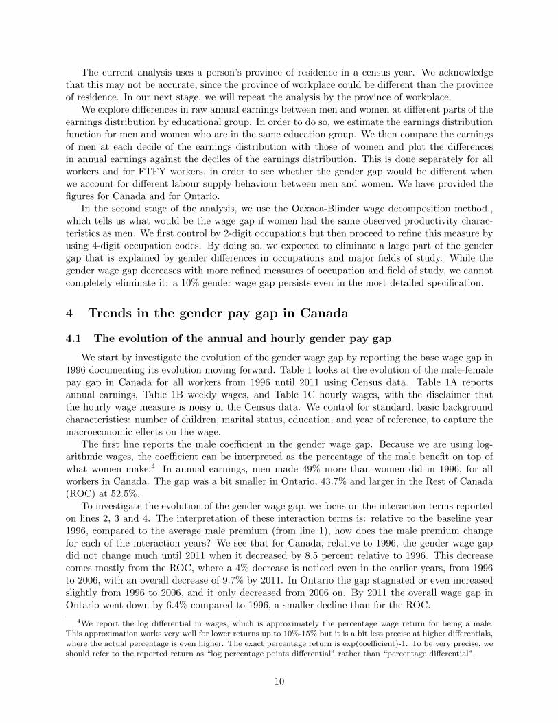
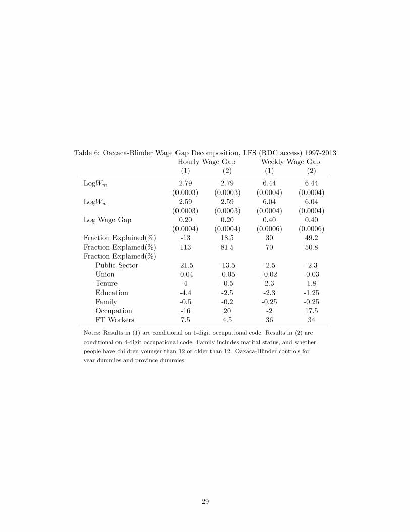
Table 6 reports the results of the Oaxaca-Blinder wage gap decomposition using the full versionof the LFS (accessed at a Research Data Centre) from 1997-2013. In this sample the total wagegap is about 20% for the hourly wage and 40% for the weekly wage. Note once again that thehourly wage gap gets amplified by the gap in hours worked between men and women, to the extentthat in weekly wages the gap is more than double. The difference between columns (1) and (2) forboth hourly and weekly wage gaps is that we use 2-digit occupational codes in columns (1), andrespectively 4-digit occupation codes in columns (2).

The only variable that can consistently explain part of the gender gap is full-time versus part-time work. Being a FT worker explains about 35% of the gender gap for weekly wages and 5%to 7.5% for hourly wage. This means that men are more likely to be full-time workers, and beinga full-time worker is associated with higher hourly wages, and even more so with higher weeklywages.

Most of the other variables cannot explain the gender wage gap, quite the opposite. Take forinstance education. Women tend to be more educated than men, and higher education is associatedwith higher wages. Due to education alone, women should earn higher wages than men, so educationwill not help explain anything from the wage gap, quite the contrary. Likewise, women are morelikely to be in the public sector or in a union, and since these characteristics are associated withhigher wages, due to these alone, women should earn more not less than men.

Other than FT status, the other two variables which can explain a bit from the gender wage gapare tenure and occupation. Tenure refers to months spent in the current job, not overall markettenure, and as such is a noisy measure of actual tenure. Still, tenure tends to explain a little bitfrom the wage gap, up to at most 4%. What makes a bigger difference for explaining the gap areoccupational characteristics. When we condition on aggregated occupations, they either explainnothing (column 1 for the weekly wage gap), or work in the opposite direction, suggesting thatwomen should have a higher wage given their occupation (column 1 for the hourly wage gap).When we condition instead on four-digit occupations, 17% to 20% of the gap gets explained. Inother words, the wage gap narrows quite a bit within a narrowly defined occupation, although alarge unexplained part still remains.

5 Heterogeneity in the pay gap by income and education

For all provinces and for both annual earnings and hourly wages, the pay gap decreases witheducation. As expected, the pay gap is much smaller for the hourly wage measure than for theannual earnings measure, with a difference of magnitudes around five or ten percentage points, andoccasionally higher.

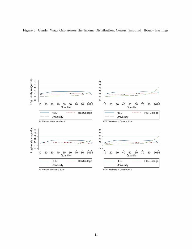
This is further confirmed by the non-parametric analysis reported in Figure 2 and Figure 3.We plot the smoothed raw wage gap across deciles of the income distribution for annual earnings(Figure 2) and hourly wages (Figure 3). We group education into three categories: (1) high-schooldrop-outs (HSD), (2) high-school and college graduates (HS+College), and (3) university includingBachelor’s and above (University). We have grouped high-school and college together because of

13

previous evidence that the human capital and returns to education for college graduates is closerto that of high-school, and even more importantly for this analysis, past research (Teng, 2015)documents a similar gender gap along all parts of the income distribution for high-school as forcollege graduates.

First, the gender gap decreases with education. The gap is highest for high-school drop-outs,followed by high-school and college, while the university group experiences the lowest gendergap.Second, we observe an increase in the gender wage gap at the highest part of the earningsdistribution for individuals with university education. We refer to this phenomenon as the glassceiling. We return to document the glass ceiling for Ontario when we do the analysis on theSunshine list in Section 7.

Third, the annual pay gender gap within education is slightly decreasing as income goes up,and it is mostly flat and smaller in magnitude when only full-time workers are considered. It ispossible that women working part-time are more likely to be better educated and earn less, thusincreasing the university wage gap when all workers are considered. It is also possible that, withinthe low educated group, part-time men still earn more than part-time women, and thus the wagegap for the low educated can be larger when part-time workers are also considered. Since thisdifference is more pronounced for the annual pay gap than for the hourly wage gap, it is possiblethat these adjustments occur on the labour supply avenue rather than on the pay gap itself.

6 Possible explanations for the remaining gender wage gap

6.1 The gender wage gap by age, marital status, and children

In the previous analysis, we could not get the hourly gender gap lower than 10%, even controllingby very refined occupations and field of study for post-secondary educated workers. Here we lookinstead at the heterogeneity in the gender wage gap separately by marital status and education.Table 7 reports the heterogeneity in the gender wage gap by marital status and age, from regressionsalso controlling for other productivity-related characteristics such as education, FT jobs, publicsector, using the public LFS, 1997 to 2014. For brevity, we only report here the mean gender wagegap within each age and marital status groups, and not the other interaction terms.

This table confirms that the gender gap is higher for married women, and it decreases witheducation and for the public sector. Most interestingly, the wage gap increases with age, at it isnot present for single women until mid-thirties. The fact that it increases with age for all maritalgroups, including single women, can be indicative of statistical discrimination. In other words, ifmarried women start losing ground relative to men as fertility choices start interfering with, say,tenure, this disadvantage will also affect single women, who get painted in terms of productivityexpectations with the same brush as married women.

A related analysis regarding the heterogeneity in the gender wage gap is reported in Table 8,using Census data and looking at the differential impact of marital status, public sector, educationand number of children on the gender wage gap. Similar conclusions from the LFS analysis carryforward, both for the aggregate wage gap decomposition, and also when decomposing the smallergender pay gaps for FTFY, FTPY and PT jobs. Being married is the biggest contributor to arelatively higher gender wage gap. Having children increases the gender pay gap, with the oneexception coming from FTPY workers with one child, for whom the hourly wage gap seems smallerthan for workers without children; this could be potentially due to the noise in our construction ofhourly wage data, especially for part-year workers.

14

6.2 The gender wage gap by public/private sectors

As reported in Table 8, workers in the public sector experience a relatively smaller wage gap.7 Public sector jobs are typically more likely to be unionized, and are also at the forefront ofimplementing equal pay and other non-discrimination measures, and a smaller gender wage gap isreflective of that.

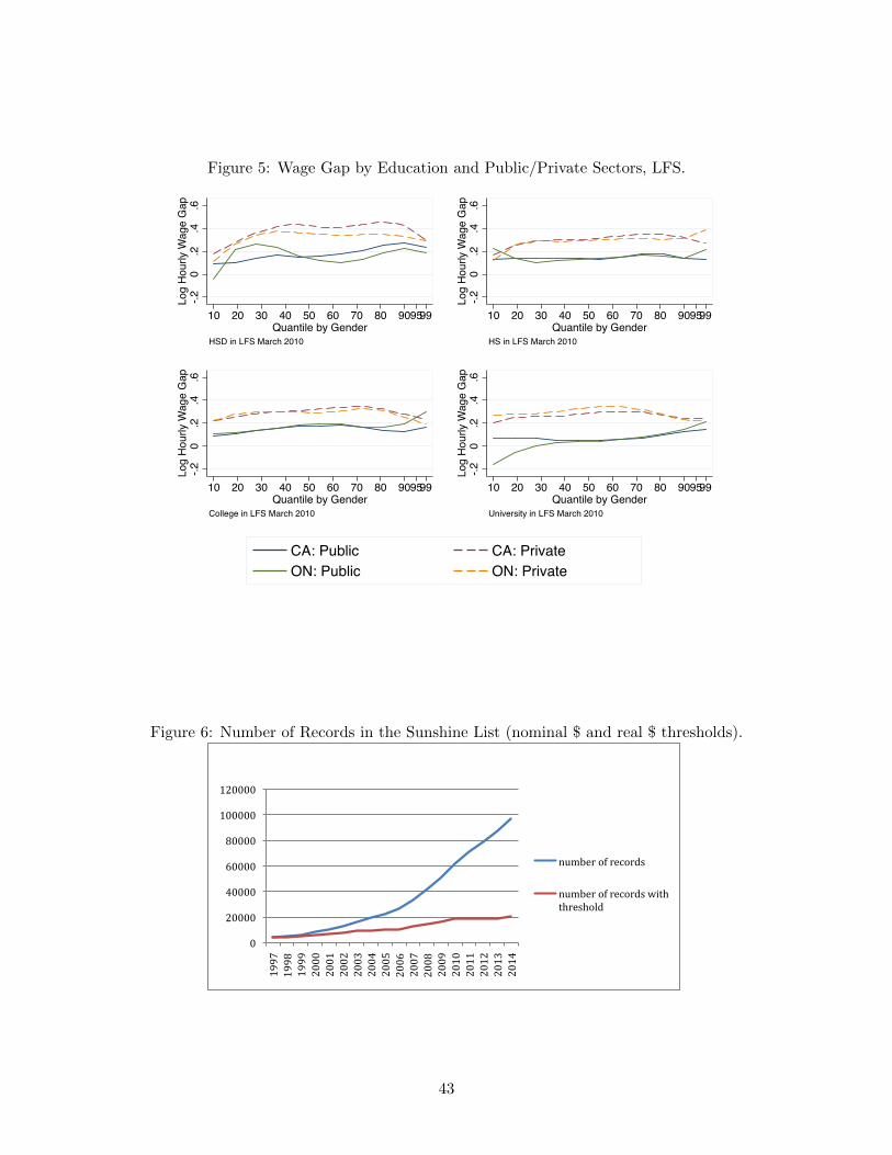
This is confirmed by Figures 4 and 5 where we look at the gender pay gap in the publicand private sectors using the hourly wage measure from the LFS, overall and also separately byeducation, along quantiles of the wage distribution. Interestingly enough, we see the gender wagegap declining at the highest wage quantiles in the private sector, but increasing in the public sector.This is also true when examining separately the gender wage gap by education levels, except forworkers with high-school education in Ontario for whom the gender wage gap seems to increaseboth in the public and the private sector at high wage levels.

Because the glass ceiling effect − higher wage gaps at high income levels − appears moreevident in the public sector, this further motivates our gender pay gap analysis for the incomes onthe Sunshine List in section 7; the Sunshine List discloses public sector incomes above a nominal$100,000 threshold.

6.3 Promotions and family/career balance

We investigate here whether any facts consistent with statistical discrimination can be docu-mented. In Table 9 we analyze the probability of promotion defined as a switch into a managerialtype of occupation. (We use the monthly panel feature of the LFS to be able to identify switchesinto managerial occupations). Men are more likely to be promoted into managerial occupationscompared to women, but, at maximum 1.5 percentage point difference, the magnitude of this effectis not that large. It is nevertheless present in both the public and private sectors, and a bit morepronounced in the private sector.

In Table 10 we document the probability of being employed in part-time work, while in Table11 we look at the probability of being absent from work within the sub-population of employedworkers. Women are more likely to be employed part-time than men are. The largest differencecomes from reasons related to caring for own children or other family. Women are 10 times morelikely to give childcare as a reason for part-time and 6 times more likely to quit a job because ofchildcare. Being single decreases the probability in both cases. Being in the public sector increasesthe probability of part-time and decreases the probability of quitting for family reasons, possiblyindicating a more family-friendly environment in the public sector.

To summarize, the labour supply channel plays a very important role in the gender pay gap,and so does the type of job (sector) and the education category. The gender wage gap increaseswith age as fertility choice and career interruptions start affecting tenure and career advancementpossibilities. There is no gender wage gap for young single people, but the gap appears fromthe thirties onward even for single childless individuals, as possible indication of the presence ofstatistical discrimination.

7A similar analysis is reported in the on-line Appendix with the separate analysis by province. The gender paygap between the public and private sectors is given by the interaction coefficient “male*public”. The gap is about10% smaller on average in the public sector for annual income, and less than that for hourly wages.

15

7 The Gender Gap and the Sunshine List

“Some believe that disclosure creates an upward salary spiral. It’s the Lake Wobegon effect. Ev-erybody wants to be above average. Employees comb through the salary disclosure lists, comparingtheir pay to that of their peers, and seeking redress for any perceived inequities. Employers tryingto attract above average workers, especially for senior management positions, offer above-averagecompensation packages, further fueling salary growth.” Frances Wooley for the Globe and Mail,March 27 2015.

The public sector salary disclosure data, better known as Ontario’s “Sunshine List”, was in-troduced in Ontario in 1997 by then-government of Mike Harris. It was designed as a mechanismto keep public salary expenditures in check, by a “public shaming of the fat cats” type of effect,by making public the names of all public sector workers earning more than $100,000 in any givenyear. To economists it is not entirely clear what sort of mechanism the government had in mind.Public knowledge of wages and salaries is something that workers and employers alike dislike, be-cause it restricts the ability of the two contractual parties to agree on remuneration reflecting theproductivity of a given worker. Indeed, while rigorous evidence is not available, anecdotal evidenceseems to indicate that the Sunshine List has had a contrary effect, of “race to the top”, becauseworkers, and in particular their unions, have used the Sunshine List to negotiate better pay fortheir members, in a “keeping up with the Jones’ ” fashion.

For our study the Sunshine List offers a unique opportunity of a glimpse at the entire populationof public sector earners in Ontario whose salaries are above the $100,000 threshold. The mainchallenge of the analysis has been identifying the gender of each respondent: while the names ofthe workers are public, their genders are not. We detail in the following section the algorithms usedin order to assign gender to each given names.

7.1 Data collection and gender assignment

The Sunshine List data used for this study was pulled from the Ontario Government public sec-tor salary disclosure website (http://www.fin.gov.on.ca/en/publications/salarydisclosure/pssd/).The gender variable is not provided in the original data, but we know what the names of in-dividuals are. In order to write computer algorithms to infer gender from first name informa-tion, we used a compiled list of names from U.S.A. Social Security data from 1950-1980 inclusive(http://www.ssa.gov/OACT/babynames/limits.html). This data provides names and gender fre-quency for all babies born in the U.S.A. in any given decade. For example, the name Lindsay hada male frequency of 5 whereas it had a female frequency of 26132; this would imply that someonenamed Lindsay had a probability of being male of 5/26134 and a probability of being female of26132/26134.

We used the information from the U.S.A. Social Security records, combined with heuristicalgorithms that decompose the characters of the first name, in order to assign a gender probabilityto each observation. We set the male threshold at an identified probability larger than .95 forthe first name to belong to a male, and likewise for the female names.8 Given this constraint,we identify a total of 197184 females and a total of 406390 males in our database, while dropping49,230 observations (7% of the original Sunshine List database of 652,804 records)when gender isassigned less precisely.

Note that this is the first attempt at processing the Sunshine List in a way that identifiesgender, even in a probabilistic way. In future research we will provide sensitivity analysis to usingthe probabilities themselves, rather than a dichotomous gender variable constructed by imposing

8More details on how the data was parsed and processed are available from the Sunshine list Appendix.

16

a threshold on the probabilities. Note though that in some of the analysis we performed so far, weexperimented with various thresholds and the results did not change substantively.

7.2 The evolution of gender shares in the Sunshine List across time

We present here some summary statistics and analysis of wages for the data on Sunshine listfrom 1997 to 2014. Note that in our analysis, the year corresponds to the year the Sunshine Listwas released, not the year of the reported income, which would be the previous calendar year (i.e.,the year 1997 on the list refers to income from 1996). Also note that the minimum salary remainedat $100,000 since the Sunshine List was introduced. We report results from two types of analysis:one taking into account all the records in the Sunshine List, with a nominal income threshold of$100,000 which does not change across this entire period, and a separate analysis where we accountfor inflation and we impose a threshold in real dollars, by deflating the nominal $100,000 by theConsumer Price Index in Ontario for each year in our data. By doing so, the income cutoff increasesover this period up to $139,456 in 2014 (referring to salary information from 2013).

There are 652,804 records in the Sunshine List to which we have assigned gender. A yearlybreakdown of the number of records is shown in Table 12, both for the actual number of recordsusing the nominal cut-off at $100,000, as well as using a real dollar cut-off income reported in column4 of that table. Figure 6 and Figure 7 report this information in a graphical way. From Figure 6 wecan see that the number of individuals on the Sunshine List has increased tremendously over thelast 15 years. The majority of the increase is due to the value of the nominal threshold becomingsmaller and smaller relative to the average salary in the economy. Put differently, part of the gap isdue to inflation, and we capture that by plotting the number of records above the inflation-adjustedthreshold. Even then, while there is some growth in the Sunshine List, we contend that it matchesthe growth in the real income in the economy, and not a relative growth in the public sector per se.

A striking point of the analysis so far is the small fraction of women relative to men who makeit on the Sunshine List. Table 12 reports in columns 3 and 6 the fraction of women on the SunshineList, and Figure 7 plots this information. The bad news is that less than a third of observations inthe Sunshine List are women. The good news is that this fraction has been increasing, from 22%females when the list was first introduced in 1997, to 36% in the 2014 list. This increase is slightlysmaller if we focus only on the subset of the Sunshine List earners who would have been on thelist even if the threshold had been moved at the pace of inflation; in that case, the percentage ofwomen increases from 22% to 31%.

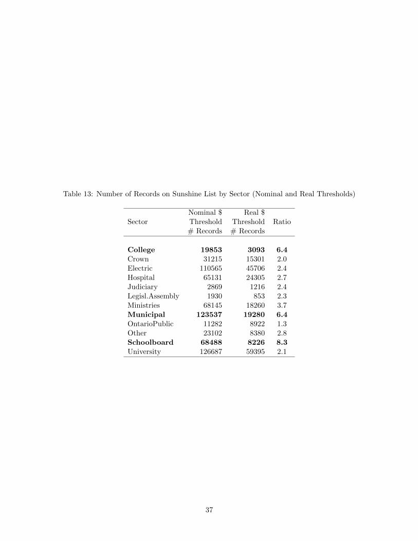
This evidence seems to indicate that, as the threshold to be nominated on the Sunshine Listkeeps decreasing in real dollar terms, more women relative to men make their way on the list.We investigate this further by analyzing separately the information by sector. Table 13 reportsthe number of observations per sector for all of the original 12 sectors that can be identified onthe Sunshine List. On average, over all sectors, there are three times more observations when thethreshold is kept at nominal $100,000 year after year. The sectors where lowering the thresholdin real terms across time makes the most difference are: the School board, Municipal sector, andColleges, where using the nominal threshold leads to an eight- or six-fold increase in the numberof records relative to the real threshold. By contrast, the size of what the Sunshine list refers to as“Ontario Public Sector” is relatively unchanged when a real threshold is imposed, as an indicationthat nominal incomes did not increase by more than inflation in this sector.

Because some of these sectors get introduced in later years, in order to try and be consistentwith relative shares of sectors across time and also to simplify the exposition in the remaininganalysis we group the sectors into five main ones: University (including College), Utilities, Hospital,School board, and Government and Judicial. Table 14 lists the percentage of women in each of these

17

sectors and across time, both for the Sunshine List using a nominal cut-off at $100,000 every year,as well as the inflation-adjusted cut-off in real dollars. The Hospital and School board sectors arethe two sectors in which women have the highest representation; since early- to mid- 2000, womenactually outnumber men in these two sectors. At the other end, women are underrepresented to ahuge extent in the Utilities sector, and this proportion has not been increasing over time.9

The main conclusion from this analysis has been that, while the percentage of women increasesover time, they are still underrepresented among the top earners in the public sector.

7.3 The gender pay gap in the Sunshine List

Figure 8 plots the male-female pay gap from the observations on the Sunshine List both usingthe nominal threshold of $100,000 and imposing the real dollar threshold on the list. The only wayto interpret these numbers is that, overall, the male-finale pay gap on the sunshine list is tiny atbest. Using the nominal threshold, the gap increases from zero in the late nineties to about 3%or 4% in current times.Although there is an increasing trend in the wage gap from 1997 to 2014,however, the wage gap is still small. When we adjust the sunshine list income threshold to accountfor inflation, the gap disappears completely. We think that the main gender gap story here comesfrom the percentage of women, rather than their earnings: only one third of people on the list arefemale, but those women who make it on the list get paid almost as much as men do and exactlyas much as men if we restrict the list to those who would have qualified under the original terms.

The slight increase in the gender pay gap under the nominal threshold, compared to no gapunder the real threshold, is consistent with the finding that individuals between the nominal andreal thresholds that is, those who wou non’t have made the list if the threshold income was adjustedfor inflation are more likely to be female. This is nevertheless not the case in all sectors, and isnot the only motivation behind the slight increase in the average pay gap on the Sunshine List.

The bottom half of Figure 8 lists the gender pay gap across the five sectors identified in theanalysis. Most of the average pay gap is coming from the Hospital sector, not only in the listusing the nominal threshold, but also in the list using the real threshold. Women who have madeit onto the Sunshine list tend to get paid, on average, as much as men do, with the exception ofthe Hospital sector. We will need to continue our research to identify where the pay gap of 20%is coming from in the Hospital sector. Another future research avenue involves the University andCollege sectors, where the trend shows an increasing pay gap.

7.4 The gender pay gap by quantiles of the income distribution

To better document glass ceiling phenomena and pay gap at the very top, we analyze differencesat quantiles of the earnings distributions for men and women respectively. Figure 9 shows theevolution of the gender pay gap at five quantiles of the earnings distribution; this way the salariesof the bottom 20% females on the Sunshine List can be compared to the salaries of the bottom20% males, and so on until the top 20%. Indeed, most of the pay gap is coming from the top 20%,consistent with the glass ceiling story where women simply don’t make it into the corner office. Itis interesting to notice though that in recent years the gap is also increasing for those at the 40th

to 60th to 80th percentile of the wage distribution. Restricting the analysis to what would amount

9One interesting observation refers to the sector where we have grouped the former government and judiciarysectors. Here, the fraction of women is higher in the real-income threshold sublist, indicating that in the mid-2000sthe women in this sector were relatively more likely to have incomes above the real threshold compared to men withincomes between the nominal and real thresholds.

18

to the same original circumstances, there was a small gap in the top quintile, but even this hasbecome smaller.

Our analysis of the Sunshine List so far supports four main conclusions. First, women areunderrepresented on the Sunshine List by a ratio of two to one. Second, those women who do makeit onto the sunshine list earn, by and large, comparable incomes with those of men. Third, while,in general, the gender pay gap does not seem to be an issue, some sectors on the Sunshine List,such as the Hospital sector, still show a substantive pay gap. Fourth, the analysis across the wagedistribution of men and women seems to indicate a glass-ceiling type of gap at the higher end ofthe respective earning distributions of men and women, consistent with our previous results.

8 Conclusion

The pay gap is a complex issue, and policy addressing it should tackle the causes of genderimbalances, and not merely attempt to fix the outcome, because that may introduce inefficiencies.Women are getting increasingly more educated and participate in record numbers in the labourforce. Current national graduation rates show that about 66% of recent post-secondary graduatesare female. Still, women are underrepresented in top occupations: two-thirds of individuals whomade it to Ontario’s Sunshine List are male.

When we discuss the gender pay gap, we must be careful in how we define this gap. The hourlywage gap is smaller than the annual wage gap. Even if the hourly wage gap were zero (which isnot) we would still observe an average gender earnings gap because women work, on average, fewerhours than men do. Subsequently, there could be two types of policies that attempt to redress thegender pay gap: one group of policies would target the difference in hours worked, while the otherwould target the remaining gap in hourly wages.

Policies that reduce the male-female gap in hours worked would be related to the availability ofhigh-quality daycare and incentives for women to return faster to work following a leave episode,in order to minimize human capital loss.

A further cultural shift in the traditional roles of men vs. women, both in the householdand in the workplace, would be a big step towards reducing gender imbalances. We have alreadyseen the huge transformation following the increased labour force participation of women in theseventies and onward. We would need a similar change of perspective in the society to even out theresponsibilities, as well as the benefits, of women and men likewise, in terms of working in the labormarket and in the household. Such a change would also help address the statistical discriminationchannel, whereby employers would no longer feel it is in their best interest to promote and encouragework from men rather than from women.

An equal society is a society where everyone has equal opportunity, and where productivity iscompensated accordingly and without discrimination. Some gender pay gap will persist even inan equal society, as long as women and men make different life-work-fertility choices. Policy canmake sure that women do not get penalized because of gender stereotypes in the work place. Anyremaining gender discrimination should go away as the society becomes fully accepting of men andwomen having an equal role in child rearing and household activities. Such decisions cannot belegislated with a heavy hand, but they can be incentivized.

19

References

[1] J. Altonji and R. Blank. Race and Gender in the Labour Market. In Handbook of LabourEconomics. D. Ashenfelter and D. Card, New York: Elsevier Science, 1999.

[2] D. Baker and M. Drolet. A new view of the male/female pay gap. Canadian Public Policy,XXXVI:429–463, 2010.

[3] D. Baker and N. Fortin. Women’s wages in women’s work: A u.s. and canada comparison ofthe roles of unions and “public goods” sector jobs. American Economic Review, 89:198–203,1999.

[4] D. Baker and N. Fortin. Occupational gender composition and wages in canada. CanadianJournal of Economics, 34:345–376, 2001.

[5] D. Baker and N. Fortin. Comparable worth in a decentralised labour market: The case ofontario. Canadian Journal of Economics, 37:850–878, 2004.

[6] M. Baker, D. Benjamin, A. Cepeg, and M. Grant. The distribution of the male/female earningsdifferential. Canadian Journal of Economics, 28:479–501, 1995.

[7] M. Baker and K. Milligan. How does job-protected maternity leave affect mothers’ employ-ment? Journal of Labour Economics, 26:no. 4: 665–691, 2008.

[8] D. Benjamin, M. Gunderson, T. Lemieux, and W. Craig Riddell. Labour Market Economics:Theory, Evidence and Policy in Canada. 7th ed. Toronto: McGraw-Hill Ryerson, 2012.

[9] S. E. Black and A. Spitz-Oener. Explaining women’s success: Technological change and theskill content of women’s work. Review of Economics and Statistics, 92:187–194, 2010.

[10] F. D. Blau and L. M. Kahn. The u.s. pay gap in the 1990s: Slowing convergence. ILR Review,60:45–60, 2006.

[11] B. Boudarbat and M. Connolly. The gender wage gap among recent post-secondary graduatesin canada: A distributional approach. Canadian Journal of Economics, 46:1037–1065, 2013.

[12] K. Cannings. Managerial promotion: The effects of socialization, specialization and gender.ILR Review, 42:77–88, 1988.

[13] V. Caponi and M. Plesca. Post-secondary education in canada: Can ability bias explain theearnings gap between college and university graduates? Canadian Journal of Economics,42:1100–1131, 2009.

[14] J. Connolly and T. Rooney. Tracking pay equity: The impact of regulatory change on thedissemination and sustainability of equal remuneration decisions. The Journal of IndustrialRelations, 54:no. 2:114–130, 2012.

[15] J. DiNardo, N. Fortin, and T. Lemieux. Labor market institutions and the distribution ofwages, 1973-1992: A semiparametric approach. Econometrica, 64:1001–1044, 1996.

[16] M. Drolet. New evidence on gender pay differentials: Does measurement matter? CanadianPublic Policy, 28:1–16, 2002a.

20

[17] M. Drolet. Can the workplace explain canadian gender pay differentials? Canadian PublicPolicy, 28:S41–S63, 2002b.

[18] M. Drolet. Why has the gender gap narrowed? Warwick Journal of Philosophy, 23:no. 1:5–16, 2011.

[19] R. Finnie and T. Wannell. Evolution of the gender earnings gap among canadian universitygraduates. Applied Economics, 36:1967–1978, 2004.

[20] S. Firpo, N. Fortin, and T. Lemuiex. Unconditional quantile regressions. Econometrica,77:953–973, 2009.

[21] R. Fisman and M. O’Neil. Gender differences in beliefs on the returns to effort: Evidence fromthe world values survey. The Journal of Human Resources, 44:no. 4: 858–70, 2009.

[22] N. Fortin and M. Huberman. Occupational gender segregation and womens wages in canada:A historical perspective. Canadian Public Policy, 28:S11S39, 2002.

[23] B. Frick. Differences in competitiveness: Empirical evidence from professional distance run-ning. Labour Economics, 18:no. 3: 389–398, 2011.

[24] C. Gerdes and P. Gransmark. Strategic behavior across gender: A comparison of female andmale expert chess players. Labour Economics, 17:no. 5: 766–775, 2010.

[25] U. Gneezy, K.L. Leonard, and J.A. List. Gender differences in competition: Evidence from amatrilineal and a patriarchal society. Econometrica, 77:no. 5: 1637–664, 2009.

[26] M. Gunderson. Gender Discrimination and Pay-Equity Legislation. In Aspects of Labour Mar-ket Behaviour: Essays in Honor of John Vanderkamp. L. Christofides, E. K. Grant, and R.Swindinsky, Toronto: University of Toronto Press, 1999.

[27] J. A. McDonald and R. J. Thornton. Coercive cooperation? ontarios pay equity act of 1988and the gender pay gap. Contemporary Economic Policy. DOI: 10.1111/coep.12094, 2014.

[28] C. B. Mulligan and Y. Rubinstein. Selection, investment, and women’s relative wages overtime. Quarterly Journal of Economics, 123:1061–1110, 2008.

[29] M. Niederie and L. Versterlund. Do women shy away from compeition? do men compete toomuch? Quarterly Journal of Economics, pages 1061–1110, 2007.

[30] Employment Equity Act. Statues of Canada 1995. c.44. s.6. laws-lois.justice.gc.ca/eng/acts/E-5.401/.

[31] Canada. Department of Labour. Employment equity. 2014. accessed march 24, 2015.http://www.labour.gc.ca/eng/standards equity/eq/emp/index.shtml.

[32] Canada. Department of Labour. Introduction to pay equity. 2013. accessed march 24, 2015.http://www.labour.gc.ca/eng/standards equity/eq/pay/intro.shtml.

[33] Ontario Human Rights Code. Statues of Ontario 1990. c.H19. http://www.e-laws.gov.on.ca/html/statutes/english/elaws statutes 90h19 e.htm#BK6.

[34] Pay Equity Act. Statues of Ontario 1990. c.P.7. s.4. http://www.e-laws.gov.on.ca/html/statutes/english/elaws statutes 90p07 e.htm#BK6.

21

[35] Employment Standards Act. Statues of Ontario 2000. c.41. s.42. http://www.e-laws.gov.on.ca/html/statutes/english/elaws statutes 00e41 e.htm#BK65.

[36] Child Care Modernization Act. Statues of Ontario 2014. c.11 s.2.http://www.ontla.on.ca/web/bills/bills detail.do?locale=en&BillID=3002.

[37] C. Olivetti and B. Petrongolo. The evolution of gender gaps in industrialized countries. NBERWorking paper, w21887.

[38] C. Olivetti and B. Petrongolo. Unequal pay or unequal employment? a cross-country analysisof gender gaps. Journal of Labor Economics, 26:621–654, 2007.

[39] K. Reilly and T. Wirjanto. Does more mean less? the male-female wage gap and the proportionof females at the establishment level. Canadian Journal of Economics, 32:906–929, 1999.

[40] T Schrile. The gender wage gap in the canadian provinces, 1997-2014. Canadian Public Policy,2015.

[41] J. Teng. Occupational characteristics and gender wage inequality: A distributional analysis.Manuscript submitted for publication, 2014.

[42] C. J. Weinberger and P.J. Kuhn. Changing levels or changing slopes? the narrowing of thegender earnings gap 1959-1999. ILR Review, 63:384–406, 2010.

[43] M. Yap and A.M. Konrad. Gender and racial differentials in promotions: Is there a stickyfloor, a mid-level bottleneck, or a glass ceiling? Industrial Relations, 64:593–619, 2009.

[44] I.U. Zeytinoglu and G.B. Cooke. Non-standard employment and promotions: a within gendersanalysis. International Relations, 50:319–337, 2008.

22

Table 1: Evolution of the Gender Pay Gap, Census 1996-2011, all jobsA. Log Annual Earnings

(1) (2) (3)Canada ROC Ontario

Males 0.491∗∗∗ 0.525∗∗∗ 0.437∗∗∗

(base 1996) (0.01) (0.01) (0.01)males*2001 −0.019 −0.036∗∗ 0.007

(0.01) (0.01) (0.02)males*2006 −0.019∗∗ −0.042∗∗∗ 0.021

(0.01) (0.01) (0.01)males*2011 −0.084∗∗ −0.097∗∗∗ −0.064∗∗∗

(0.01) (0.01) (0.01)Intercept 123∗∗ 129∗∗∗ 233∗∗∗

(0.01) (0.01) (0.02)

B. Log Weekly Wage

(1) (2) (3)Canada ROC Ontario

Males 0.363∗∗∗ 0.385∗∗∗ 0.327∗∗∗

(base 1996) (0.01) (0.01) (0.01)males*2001 −0.017∗ −0.033∗∗ 0.007

(0.01) (0.01) (0.01)males*2006 0.021∗∗∗ 0.005 0.049∗∗∗

(0.01) (0.01) (0.01)males*2011 −0.026∗∗∗ −0.033∗∗∗ −0.014

(0.01) (0.01) (0.01)Intercept 4.383∗∗∗ 4.389∗∗∗ 4.468∗∗∗

(0.01) (0.01) (0.02)

C. Log Hourly Wage

(1) (2) (3)Canada ROC Ontario

Males 0.155∗∗∗ 0.169∗∗∗ 0.134∗∗∗

(base 1996) (0.01) (0.01) (0.01)males*2001 0.023∗∗ 0.008 0.045∗∗

(0.01) (0.01) (0.01)males*2006 0.064∗∗∗ 0.050∗∗∗ 0.086∗∗∗

(0.01) (0.01) (0.01)males*2011 0.048∗∗∗ 0.042∗∗∗ 0.057∗∗∗

(0.01) (0.01) (0.01)Intercept 1.123∗∗∗ 1.129∗∗∗ 1.233∗∗∗

(0.01) (0.01) (0.02)

Standard errors in parentheses.∗ p < 0.05, ∗∗ p < 0.01, ∗∗∗ p < 0.001

23

Table 2: Evolution of the Gender Pay Gap, Census 1996-2011, FTFYA. Log Annual Earnings, FTFY workers

(1) (2) (3)Canada ROC Ontario

Males 0.267∗∗∗ 0.285∗∗∗ 0.243∗∗∗

(base 1996) (0.01) (0.01) (0.01)males*2001 0.012 0.005 0.021

(0.01) (0.01) (0.01)males*2006 0.044∗∗∗ 0.032∗∗∗ 0.062∗∗∗

(0.01) (0.01) (0.01)males*2011 0.011 0.006 0.015

(0.01) (0.01) (0.01)Intercept 8.519∗∗∗ 8.529∗∗∗ 8.627∗∗∗

(0.01) (0.01) (0.02)

B. Log Weekly Wage, FTFY workers

(1) (2) (3)Canada ROC Ontario

Males 0.266∗∗∗ 0.285∗∗∗ 0.242∗∗∗

(base 1996) (0.01) (0.01) (0.01)males*2001 0.012∗ 0.005 0.021

(0.01) (0.01) (0.01)males*2006 0.045∗∗∗ 0.032∗∗∗ 0.062∗∗∗

(0.01) (0.01) (0.01)males*2011 0.011 0.006 0.016

(0.01) (0.01) (0.01)Intercept 4.587∗∗∗ 4.598∗∗∗ 4.695∗∗∗

(0.01) (0.01) (0.02)

C. Log Hourly Wage, FTFY workers

(1) (2) (3)Canada ROC Ontario

Males 0.160∗∗∗ 0.173∗∗∗ 0.143∗∗∗

(base 1996) (0.01) (0.01) (0.01)males*2001 0.022∗ 0.007 0.044∗∗

(0.01) (0.01) (0.02)males*2006 0.046∗∗∗ 0.055∗∗∗ 0.078∗∗∗

(0.01) (0.01) (0.01)males*2011 0.051∗∗∗ 0.047∗∗∗ 0.055∗∗∗

(0.01) (0.01) (0.01)Intercept 1.025∗∗∗ 1.035∗∗∗ 1.130∗∗∗

(0.01) (0.01) (0.02)

Standard errors in parentheses.∗ p < 0.05, ∗∗ p < 0.01, ∗∗∗ p < 0.001

24

Table 3: Evolution of the Gender Pay Gap, Census 1996-2011, FT Part YearA. Log Annual Earnings, FT Part Year Workers

(1) (2) (3)Canada ROC Ontario

Males 0.313∗∗∗ 0.356∗∗∗ 0.230∗∗∗

(base 1996) (0.01) (0.01) (0.02)males*2001 0.017 −0.010 0.069∗

(0.02) (0.02) (0.03)males*2006 0.050∗∗∗ 0.035∗ 0.088∗∗∗

(0.01) (0.01) (0.02)males*2011 −0.009 −0.015 0.003

(0.01) (0.02) (0.02)Intercept 7.280∗∗∗ 7.227∗∗∗ 7.747∗∗∗

(0.03) (0.03) (0.04)

B. Log Weekly Wage, FT Part Year Workers

(1) (2) (3)Canada ROC Ontario

Males 0.275∗∗∗ 0.308∗∗∗ 0.208∗∗∗

(base 1996) (0.01) (0.01) (0.02)males*2001 −0.010∗ −0.032 0.030

(0.02) (0.02) (0.03)males*2006 0.006 −0.004 0.033

(0.01) (0.01) (0.02)males*2011 −0.024∗ −0.030∗ −0.011

(0.01) (0.01) (0.02)Intercept 4.945∗∗∗ 4.892∗∗∗ 5.163∗∗∗

(0.02) (0.03) (0.04)

C. Log Hourly Wage, FT Part Year Workers

(1) (2) (3)Canada ROC Ontario

Males 0.121∗∗∗ 0.151∗∗∗ 0.063∗∗

(base 1996) (0.01) (0.02) (0.02)males*2001 0.007 −0.007 0.026

(0.02) (0.02) (0.03)males*2006 0.049∗∗∗ 0.035∗ 0.083∗∗∗

(0.01) (0.02) (0.02)males*2011 0.045∗∗ 0.038∗ 0.061∗

(0.01) (0.02) (0.02)Intercept 1.362∗∗∗ 1.321∗∗∗ 1.621∗∗∗

(0.03) (0.03) (0.05)

Standard errors in parentheses.∗ p < 0.05, ∗∗ p < 0.01, ∗∗∗ p < 0.001

25

Table 4: Evolution of the Gender Pay Gap, Census 1996-2011, Part TimeA. Log Annual Earnings, PT Workers

(1) (2) (3)Canada ROC Ontario

Males 0.221∗∗∗ 0.244∗∗∗ 0.175∗∗∗

(base 1996) (0.02) (0.03) (0.04)males*2001 0.027 0.014 0.053

(0.03) (0.04) (0.06)males*2006 −0.189∗∗∗ −0.194∗∗∗ −0.175∗∗∗

(0.02) (0.03) (0.04)males*2011 −0.179∗∗∗ −0.188∗∗∗ −0.159∗∗∗

(0.02) (0.03) (0.04)Intercept 6.937∗∗∗ 6.759∗∗∗ 7.441∗∗∗

(0.04) (0.04) (0.06)

B. Log Weekly Wage, PT Workers

(1) (2) (3)Canada ROC Ontario

Males 0.216∗∗∗ 0.234∗∗∗ 0.176∗∗∗

(base 1996) (0.02) (0.02) (0.03)males*2001 0.008∗ −0.016 0.054

(0.03) (0.03) (0.05)males*2006 −0.118∗∗∗ −0.119∗∗∗ −0.111∗∗∗

(0.02) (0.02) (0.03)males*2011 −0.105∗∗∗ −0.111∗∗∗ −0.085∗

(0.02) (0.02) (0.03)Intercept 4.631∗∗∗ 4.472∗∗∗ 4.887∗∗∗

(0.03) (0.04) (0.05)

C. Log Hourly Wage, PT Workers

(1) (2) (3)Canada ROC Ontario

Males −0.002 0.012 −0.033(base 1996) (0.02) (0.03) (0.04)males*2001 0.097∗∗ 0.088∗ 0.116

(0.04) (0.04) (0.06)males*2006 −0.017 −0.019 −0.009

(0.03) (0.03) (0.04)males*2011 0.002 −0.004 0.022

(0.03) (0.03) (0.04)Intercept 1.604∗∗∗ 1.503∗∗∗ 1.826∗∗∗

(0.04) (0.04) (0.06)

Standard errors in parentheses.∗ p < 0.05, ∗∗ p < 0.01, ∗∗∗ p < 0.001

26

Table 5: Evolution of the Gender Pay Gap, Public LFS, Hourly Wages

A. Basic Pay Gap (unconditional)

Year CANADA ONTARIO ROC

1997 0.77 0.77 0.771998 0.77 0.77 0.771999 0.77 0.77 0.772000 0.77 0.77 0.772001 0.77 0.76 0.782002 0.78 0.78 0.782003 0.79 0.78 0.792004 0.80 0.79 0.802005 0.81 0.81 0.822006 0.81 0.81 0.822007 0.81 0.81 0.822008 0.82 0.82 0.822009 0.83 0.83 0.832010 0.84 0.85 0.842011 0.85 0.86 0.852012 0.84 0.86 0.842013 0.84 0.86 0.842014 0.85 0.86 0.86

B. Conditional Pay Gap: adding age, education,tenure, industry and occupation, and year

and province indicators.

Year CANADA ONTARIO ROC

1997 0.83 0.84 0.831998 0.83 0.84 0.831999 0.84 0.84 0.842000 0.83 0.84 0.832001 0.83 0.83 0.832002 0.84 0.85 0.842003 0.84 0.84 0.832004 0.85 0.86 0.842005 0.86 0.86 0.862006 0.86 0.85 0.872007 0.86 0.85 0.862008 0.86 0.86 0.862009 0.87 0.88 0.86 0.87 0.87 0.882010 0.87 0.88 0.87 0.87 0.87 0.882011 0.88 0.89 0.88 0.89 0.88 0.902012 0.88 0.89 0.87 0.88 0.88 0.892013 0.88 0.89 0.87 0.88 0.88 0.892014 0.88 0.89 0.87 0.88 0.88 0.89

C. Conditional Pay Gap: adding Familycharacteristics (marital status, children) to

age, education, tenure, industry, occupation,year and province indicators.

Year CANADA ONTARIO ROC

1997 0.84 0.84 0.831998 0.83 0.84 0.831999 0.84 0.84 0.842000 0.83 0.84 0.832001 0.83 0.83 0.832002 0.84 0.85 0.842003 0.84 0.84 0.832004 0.85 0.86 0.842005 0.86 0.86 0.862006 0.86 0.85 0.872007 0.86 0.85 0.862008 0.86 0.86 0.86

27

Table 5 (cont). Evolution of the Gender Pay Gap,Public LFS, Hourly Wages

Year CANADA ONTARIO ROC

2009 0.87 0.88 0.86 0.87 0.87 0.882010 0.87 0.88 0.87 0.88 0.87 0.882011 0.88 0.89 0.88 0.89 0.88 0.902012 0.88 0.89 0.87 0.88 0.88 0.892013 0.88 0.89 0.87 0.88 0.88 0.892014 0.88 0.89 0.87 0.88 0.88 0.89

Note: After 2009 we can control for 4-digit refinedoccupational codes (columns 3, 5, and 7)

28

Table 6: Oaxaca-Blinder Wage Gap Decomposition, LFS (RDC access) 1997-2013Hourly Wage Gap Weekly Wage Gap(1) (2) (1) (2)

LogWm 2.79 2.79 6.44 6.44(0.0003) (0.0003) (0.0004) (0.0004)

LogWw 2.59 2.59 6.04 6.04(0.0003) (0.0003) (0.0004) (0.0004)

Log Wage Gap 0.20 0.20 0.40 0.40(0.0004) (0.0004) (0.0006) (0.0006)

Fraction Explained(%) -13 18.5 30 49.2Fraction Explained(%) 113 81.5 70 50.8Fraction Explained(%)

Public Sector -21.5 -13.5 -2.5 -2.3Union -0.04 -0.05 -0.02 -0.03Tenure 4 -0.5 2.3 1.8Education -4.4 -2.5 -2.3 -1.25Family -0.5 -0.2 -0.25 -0.25Occupation -16 20 -2 17.5FT Workers 7.5 4.5 36 34

Notes: Results in (1) are conditional on 1-digit occupational code. Results in (2) are

conditional on 4-digit occupational code. Family includes marital status, and whether

people have children younger than 12 or older than 12. Oaxaca-Blinder controls for

year dummies and province dummies.

29

Table 7: Heterogeneity in the wage gap by marital status and age groups, controlling byeducation and job type. Public LFS, 1997 to 2014

MARRIED DIVORCED, WIDOWED SINGLE

Coef. Std. Err. Coef. Std. Err. Coef. Std. Err.

Overall No Interaction -0.178 0.001 -0.150 0.002 -0.072 0.001

Overall w/ InteractionGender Gap -0.136 0.002 -0.124 0.006 -0.048 0.005

Age 25 to 26Gender gap -0.015 0.015 -0.07 0.079 0.037 0.013

Age 27 to 29Gender gap -0.035 0.012 -0.154 0.043 0.027 0.013

Age 30 to 34Gender gap -0.075 0.008 -0.010 0.026 -0.033 0.012

Age 35 to 39Gender gap -0.094 0.008 -0.132 0.020 -0.041 0.013

Age 40 to 44Gender gap -0.121 0.007 -0.121 0.016 -0.120 0.014

Age 45 to 49Gender gap -0.186 0.007 -0.136 0.015 -0.093 0.016

Age 50 to 54Gender gap -0.175 0.006 -0.178 0.015 -0.119 0.019

Age 55 to 59Gender gap -0.135 0.006 -0.099 0.015 -0.012 0.023

Age 60 to 64Gender gap -0.121 0.008 -0.085 0.017 -0.138 0.032

30

Table 8: Relative Gender Wage Gap, Census

Weekly Hourly

Canada Ontario ROC Canada Ontario ROC

Panel A: All Workers

Relative to SingleMarried 0.125∗∗∗ 0.134∗∗∗ 0.128∗∗∗ 0.076∗∗∗ 0.084∗∗∗ 0.074∗∗∗

Other 0.063∗∗∗ 0.070∗∗∗ 0.065∗∗∗ 0.057∗∗∗ 0.057∗∗∗ 0.059∗∗∗

Relative to Private SectorPublic Sector −0.089∗∗∗ −0.088∗∗ −0.092∗∗∗ −0.056∗∗∗ −0.057∗∗∗ −0.056∗∗∗

Relative to HSCollege −0.022∗∗∗ −0.012∗∗ −0.026∗∗∗ −0.020∗∗∗ −0.022∗∗∗ −0.019∗∗∗

University −0.101∗∗∗ −0.082∗∗∗ −0.109∗∗∗ −0.088∗∗∗ −0.084∗∗∗ −0.091∗∗∗

Relative to without Childrenwith one child 0.049∗∗∗ 0.040∗∗∗ 0.055∗∗∗ 0.038∗∗∗ 0.032∗∗∗ 0.041∗∗∗

with 2+ children 0.079∗∗∗ 0.078∗∗∗ 0.081∗∗∗ 0.049∗∗∗ 0.051∗∗∗ 0.047∗∗∗

Panel B: Full Time Part Year Workers

Relative to SingleRelative to Single

Married 0.111∗∗∗ 0.108∗∗∗ 0.126∗∗∗ 0.066∗∗∗ 0.063∗∗∗ 0.076∗∗∗

Other 0.058∗∗∗ 0.049∗∗∗ 0.070∗∗∗ 0.042∗∗∗ 0.032∗∗ 0.053∗∗∗

Relative to Private SectorPublic Sector −0.050∗∗∗ −0.032∗∗ −0.060∗∗∗ −0.025∗∗∗ −0.008 −0.035∗∗∗

Relative to HSCollege −0.053∗∗∗ −0.045∗∗ −0.053∗∗∗ −0.055∗∗∗ −0.053∗∗∗ −0.057∗∗∗

University −0.232∗∗∗ −0.234∗∗∗ −0.219∗∗∗ −0.208∗∗∗ −0.216∗∗∗ −0.199∗∗∗

Relative to without Childrenwith one child −0.015∗∗∗ −0.017 −0.009 −0.035∗∗∗ −0.040∗∗∗ −0.030∗∗∗

with 2+ children 0.036∗∗∗ 0.031∗∗∗ 0.043∗∗∗ 0.022∗∗∗ 0.019∗ 0.26∗∗∗

Panel C: Full Time Full Year Workers

Relative to SingleMarried 0.120∗∗∗ 0.136∗∗∗ 0.119∗∗∗ 0.094∗∗∗ 0.103∗∗∗ 0.092∗∗∗

Other 0.047∗∗∗ 0.058∗∗∗ 0.045∗∗∗ 0.050∗∗∗ 0.054∗∗∗ 0.050∗∗∗

Relative to Private SectorPublic Sector −0.087∗∗∗ −0.088∗∗∗ −0.089∗∗∗ −0.058∗∗∗ −0.061∗∗∗ −0.058∗∗∗

Relative to HSCollege −0.028∗∗∗ −0.026∗∗∗ −0.028∗∗∗ −0.026∗∗∗ −0.033∗∗∗ −0.023∗∗∗

University −0.098∗∗∗ −0.083∗∗∗ −0.106∗∗∗ −0.081∗∗∗ −0.077∗∗∗ −0.084∗∗∗

Relative to without Childrenwith one child 0.067∗∗∗ 0.056∗∗∗ 0.074∗∗∗ 0.050∗∗∗ 0.043∗∗∗ 0.054∗∗∗

with 2+ children 0.085∗∗∗ 0.085∗∗∗ 0.086∗∗∗ 0.055∗∗∗ 0.057∗∗∗ 0.055∗∗∗

Panel D: Part Time Workers

Relative to SingleMarried 0.059∗∗∗ 0.031∗∗ 0.081∗∗∗ −0.073∗∗∗ −0.113∗∗∗ −0.048∗∗∗

Other 0.070∗∗∗ 0.040∗ 0.875∗∗∗ 0.047∗∗∗ −0.016 0.081∗∗∗

Relative to Private SectorPublic Sector −0.050∗∗∗ −0.060∗∗ −0.050∗∗∗ −0.027∗∗ 0.035∗ 0.017

Relative to HSCollege −0.009 0.065∗∗∗ −0.042∗∗∗ −0.019 0.031 −0.043∗∗

University −0.118∗∗∗ −0.023 −0.161∗∗∗ −0.151∗∗∗ −0.106∗∗∗ −0.171∗∗∗

31

Relative to without Childrenwith one child 0.045∗∗∗ 0.021 0.061∗∗∗ −0.008 −0.019 0.001with 2+ children 0.049∗∗∗ 0.045∗∗∗ 0.054∗∗∗ −0.049∗∗∗ −0.050∗∗∗ −0.048∗∗∗

Standard errors in parentheses.∗ p < 0.05, ∗∗ p < 0.01, ∗∗∗ p < 0.001

32

Table 9: Probability of promotion by genderAll Workers All Workers Single Not Single Women Men

Public Private Public Private Public Private

Male 0.012∗∗∗ 0.009∗∗∗ 0.012∗∗∗ 0.008∗∗∗ 0.006∗∗∗ 0.009∗∗∗ 0.015∗∗∗ Public −0.005∗∗∗ −0.082∗∗∗

(0.0004) (0.001) (0.0005) (0.002) (0.001) (0.001) (0.0006) (0.0007) (0.0009)

Age 0.003∗∗∗ 0.002∗∗∗ 0.003∗∗∗ 0.005∗∗∗ 0.004∗∗∗ −0.0007∗ 0.003∗∗∗ Age 0.003∗∗∗ 0.004∗∗∗

(0.0002) (0.0003) (0.0002) (0.0006) (0.0003) (0.0004) (0.0003) (0.0003) (0.0002)

Age2 −0.00004∗∗∗ −0.00002∗∗∗ −0.00004∗∗∗ −0.00006∗∗∗ −0.00006∗∗∗ 0.000007 −0.00003∗∗∗ Age2 −0.00004∗∗∗ −0.00004∗∗∗

(0.000001) (0.000003) (0.000001) (0.000003) (0.000003) (0.000005) (0.000003) (0.000003) (0.000002)

Married −0.001∗∗∗ −0.003∗∗∗ −0.0005 −0.006∗∗∗ −0.003∗∗∗ Married −0.004∗∗∗ 0.001(0.0006) (0.001) (0.0006) (0.002) (0.001) (0.0007) (0.001)

Divorced/ 0.002∗∗ 0.0005 0.002∗∗ Divorced/ 0.0002 0.004∗∗

Widowed (0.001) (0.002) (0.001) Widowed (0.001) (0.001)

HS 0.008∗∗∗ 0.01∗∗∗ 0.009∗∗∗ 0.005 0.004∗∗∗ 0.009∗∗∗ 0.009∗∗∗ HS 0.007∗∗∗ 0.009∗∗∗

(0.0007) (0.003) (0.0007) (0.001) (0.001) (0.003) (0.001) (0.0008) (0.001)

College 0.008∗∗∗ −0.003 0.009∗∗∗ −0.006 0.009∗∗∗ −0.005 0.008∗∗∗ College 0.008∗∗∗ 0.009∗∗∗

(0.0007) (0.003) (0.0007) (0.003) (0.003) (0.003) (0.001) (0.0008) (0.001)

University 0.01∗∗∗ −0.004 0.02∗∗∗ −0.01∗∗ 0.020∗∗∗ −0.006∗ 0.02∗∗∗ University 0.014∗∗∗ 0.02∗∗∗

(0.0008) (0.003) (0.0008) (0.005) (0.001) (0.003) (0.001) (0.0009) (0.001)

cons −0.04∗∗∗ −0.009 −0.04∗∗∗ −0.06∗∗∗ −0.06∗∗∗ 0.05∗∗∗ −0.03 cons −0.03∗∗∗ −0.04∗∗∗

(0.002) (0.001) (0.002) (0.01) (0.003) (0.009) (0.004) (0.002) (0.002)

# of obs. 737516 133577 603939 28146 194737 105431 409202 # of obs. 374398 363118Standard errors in parentheses.∗ p < 0.05, ∗∗ p < 0.01, ∗∗∗ p < 0.001

Table 10: Probability of Working Part-time and Probability of Leaving Job Due to Children andFamily Obligations. Source: 2013 public LFSA. Tabulations from the data

Reason for part-time % for Males % for Females Reason why left job % for Males % for Females

Other reasons 2.64 2.11 Left job-other reasons 9.99 12.85Own illness/disability 4.35 4.14 Left job-illness/disab 5.34 5.99Care for own children 1.39 12.67 Left job-person/family 1.40 7.61Other family 1.32 3.58Going to school 34.72 23.36 Left job-school 20.25 20.15Personal preference 7.78 27.82Couldn’t find FT/look 10.54 9.02 Lost job: laid off 53.41 42.76Couldn’t find FT/didn’t 17.26 17.31 Left job: retired 9.61 10.65

Total 46881 97602 Total 52639 47872

B. Regression Coefficients for the Probability of Part-time/Probability of Leaving Job Due to Childrenand Family Obligations

Probability (PART-TIME) Probability (LEAVING JOB)

Women 0.135 Women 0.062Intercept 0.02 Intercept 0.014

No regressors included.

Women 0.119 Women 0.075Public Sector 0.001 Public Sector 0.007Women*Public 0.009 Women*Public -0.029Single -0.072 Single -0.047Women*Single -0.101 Women*Single -0.048Union -0.015

Also included are age, education, province, industry, and occupation.

34

Table 11: Probability of Being Employed Absent from WorkSample average

Male 0.073Female 0.104

Coef. Std. Err. Coef. Std. Err.

FEMALE 0.032 0.0002 FEMALE 0.003 0.0002age 27-30 0.015 0.0005 younger 3 0.003 0.0004age 30-34 0.021 0.0005 younger 5 -0.003 0.0005age 35-39 0.006 0.0005 younger 12 -0.002 0.0004age 40-44 -0.000 0.0005 younger 15 -0.002 0.0004age 45-49 0.005 0.0005 mom younger 3 0.222 0.0006age 50-54 0.013 0.0005 mom younger 5 0.014 0.0007age 55-59 0.020 0.0005 mom younger 12 0.005 0.0005age 60-65 0.027 0.0006 public 0.029 0.0003intercept 0.029 0.0005 public*FEMALE 0.017 0.0004

age 27-30 0.006 0.0005age 30-34 0.008 0.0005age 35-39 0.008 0.0005age 40-44 0.013 0.0005age 45-49 0.020 0.0005

Coef. Std. Err. age 50-54 0.028 0.0005FEMALE 0.26 00002. age 55-59 0.036 0.0005public 0.040 0.0002 age 60-65 0.043 0.0006intercept 0.040 0.0003 intercept 0.050 0.0004

35

Table 12: Number of Records on Sunshine List (Nominal and Real Thresholds)

Nominal $ Threshold Real $ ThresholdYear Nb. Records % female Constant $ Cut-off Nb. Records % female

1997 4307 0.22 $100,000 4307 0.221998 4866 0.24 $101,814 4445 0.241999 6210 0.23 $102,721 5332 0.232000 8008 0.20 $104,762 6168 0.212001 10331 0.21 $107,823 6751 0.212002 12973 0.24 $111,111 7873 0.242003 16237 0.24 $113,379 9369 0.242004 19947 0.25 $116,440 9404 0.252005 22387 0.26 $118,594 9730 0.252006 26694 0.28 $121,202 10524 0.262007 33618 0.29 $123,356 12796 0.272008 41920 0.31 $125,624 14505 0.272009 50383 0.32 $128,458 16359 0.282010 61496 0.34 $128,912 19068 0.292011 71052 0.35 $132,086 18971 0.292012 78910 0.36 $136,168 18564 0.302013 86941 0.37 $138,095 18708 0.312014 96524 0.36 $139,456 20063 0.31

Total 652804 212937

36

Table 13: Number of Records on Sunshine List by Sector (Nominal and Real Thresholds)

Nominal $ Real $Sector Threshold Threshold Ratio

# Records # Records

College 19853 3093 6.4Crown 31215 15301 2.0Electric 110565 45706 2.4Hospital 65131 24305 2.7Judiciary 2869 1216 2.4Legisl.Assembly 1930 853 2.3Ministries 68145 18260 3.7Municipal 123537 19280 6.4OntarioPublic 11282 8922 1.3Other 23102 8380 2.8Schoolboard 68488 8226 8.3University 126687 59395 2.1

37

Table 14: Percent women across time and (aggregated) sectorsA. Nominal income threshold ($100,000)year Univ&College Utilities Hospital GVT&Judicial Schlboard overall

1997 0.11 0.25 0.29 0.26 0.20 0.211998 0.13 0.20 0.33 0.29 0.25 0.241999 0.13 0.19 0.32 0.28 0.29 0.222000 0.14 0.12 0.32 0.30 0.33 0.202001 0.15 0.13 0.38 0.29 0.38 0.212002 0.18 0.13 0.43 0.33 0.37 0.232003 0.20 0.13 0.45 0.30 0.40 0.242004 0.23 0.12 0.50 0.29 0.41 0.242005 0.25 0.12 0.51 0.29 0.47 0.262006 0.27 0.12 0.53 0.28 0.50 0.282007 0.30 0.13 0.57 0.27 0.52 0.292008 0.32 0.13 0.62 0.27 0.55 0.312009 0.33 0.15 0.67 0.26 0.56 0.322010 0.35 0.17 0.67 0.27 0.57 0.342011 0.36 0.17 0.67 0.27 0.57 0.352012 0.38 0.18 0.69 0.28 0.57 0.362013 0.39 0.16 0.70 0.28 0.57 0.372014 0.40 0.19 0.69 0.27 0.57 0.36

Total 0.33 0.15 0.63 0.28 0.55 0.33

B. Real $ Income Thresholdyear Univ&College Utilities Hospital GVT&Judicial Schlboard overall

1997 0.11 0.25 0.29 0.26 0.20 0.211998 0.13 0.20 0.32 0.29 0.25 0.241999 0.13 0.19 0.32 0.28 0.30 0.232000 0.14 0.11 0.31 0.30 0.33 0.212001 0.16 0.13 0.35 0.29 0.37 0.212002 0.17 0.13 0.39 0.33 0.34 0.232003 0.19 0.14 0.40 0.30 0.34 0.242004 0.20 0.13 0.42 0.32 0.39 0.242005 0.21 0.12 0.42 0.32 0.43 0.252006 0.22 0.13 0.42 0.31 0.46 0.252007 0.25 0.13 0.46 0.32 0.47 0.272008 0.25 0.13 0.49 0.33 0.46 0.272009 0.27 0.14 0.52 0.33 0.46 0.282010 0.28 0.14 0.51 0.34 0.51 0.292011 0.29 0.14 0.50 0.34 0.52 0.292012 0.29 0.15 0.50 0.35 0.52 0.302013 0.31 0.13 0.51 0.36 0.49 0.312014 0.32 0.15 0.50 0.35 0.48 0.31

Total 0.25 0.14 0.45 0.33 0.43 0.27

38

Figure 1: Evolution of the Gender Wage Gap, Canada (Census)..2

.25

.3.3

5Lo

g A

nnua

l Wag

e G

ap

1995 2000 2005 2010Year

Canada ROCOntario

25-64 full-time full-year workers.2

.25

.3.3

5.4

Log

Ann

ual W

age

Gap

1995 2000 2005 2010Year

Canada ROCOntario

25-64 full-time part-year workers

0.0

5.1

.15

.2.2

5Lo

g A

nnua

l Wag

e G

ap

1995 2000 2005 2010Year

Canada ROCOntario

25-64 part-time workers

39

Figure 2: Gender Wage Gap Across the Income Distribution, Census Annual Earnings.

0.1

.2.3

.4.5

.6Lo

g An

nual

Ear

ning

s G

ap

10 20 30 40 50 60 70 80 9095Quantile

HSD HS+College University

All Workers in Canada 2010

0.1

.2.3

.4.5

.610 20 30 40 50 60 70 80 9095

Quantile

HSD HS+College University

FTFY Workers in Canada 2010

0.1

.2.3

.4.5

.6Lo

g An

nual

Ear

ning

s G

ap

10 20 30 40 50 60 70 80 9095Quantile

HSD HS+College University

All Workers in Ontario 2010

.1.2

.3.4

.5.6

10 20 30 40 50 60 70 80 9095Quantile

HSD HS+College University

FTFY Workers in Ontario 2010

40

Figure 3: Gender Wage Gap Across the Income Distribution, Census (imputed) Hourly Earnings.

0.1

.2.3

.4.5

.6Lo

g H

ourly

Wag

e G

ap

10 20 30 40 50 60 70 80 9095Quantile

HSD HS+College University

All Workers in Canada 2010

0.1

.2.3

.4.5

.610 20 30 40 50 60 70 80 9095

Quantile

HSD HS+College University

FTFY Workers in Canada 2010

0.1

.2.3

.4.5

.6Lo

g H

ourly

Wag

e G

ap

10 20 30 40 50 60 70 80 9095Quantile

HSD HS+College University

All Workers in Ontario 2010

0.1

.2.3

.4.5

.6

10 20 30 40 50 60 70 80 9095Quantile

HSD HS+College University

FTFY Workers in Ontario 2010

41

Figure 4: Wage Gap by Public/Private Sectors, LFS.

0.1

.2.3

.4Lo

g Ho

urly

Wag

e G

ap

10 20 30 40 50 60 70 80 90 95 99Quantile by Gender

CA: Public CA: PrivateON: Public ON: Private

People aged between 25 and 64 in LFS March 2010

42

Figure 5: Wage Gap by Education and Public/Private Sectors, LFS.

-.20

.2.4

.6Lo

g Ho

urly

Wag

e G

ap

10 20 30 40 50 60 70 80 909599Quantile by Gender

HSD in LFS March 2010

-.20

.2.4

.6Lo

g Ho

urly

Wag

e G

ap

10 20 30 40 50 60 70 80 909599Quantile by Gender

HS in LFS March 2010

-.20

.2.4

.6Lo

g Ho

urly

Wag

e G

ap

10 20 30 40 50 60 70 80 909599Quantile by Gender

College in LFS March 2010

-.20

.2.4

.6Lo

g Ho

urly

Wag

e G

ap

10 20 30 40 50 60 70 80 909599Quantile by Gender

University in LFS March 2010

CA: Public CA: PrivateON: Public ON: Private

Figure 6: Number of Records in the Sunshine List (nominal $ and real $ thresholds).

0  

20000  

40000  

60000  

80000  

100000  

120000  

1997  

1998  

1999  

2000  

2001  

2002  

2003  

2004  

2005  

2006  

2007  

2008  

2009  

2010  

2011  

2012  

2013  

2014  

number  of  records  

number  of  records  with  threshold  

43

Figure 7: Evolution of the Gender Ratio in the Sunshine List (nominal $ and real $ thresholds).

0.2  

0.22  

0.24  

0.26  

0.28  

0.3  

0.32  

0.34  

0.36  

0.38  

1997   1998   1999   2000   2001   2002   2003   2004   2005   2006   2007   2008   2009   2010   2011   2012   2013   2014  

Nominal  

Real  

44

Figure 8: Pay Gap between Men and Women in the Sunshine List.

-.05

0.0

5.1

1995 2000 2005 2010 2015year

All Sectors Smoothened plot

Male-Female % Income DifferentialSunshine List

-.05

0.0

5.1

1995 2000 2005 2010 2015year

All Sectors Smoothened plot

Male-Female % Income DifferentialSunshine List, Real Threshold

-.05

0.0

5.1

.15

.2

1995 2000 2005 2010 2015year

University Utilities HospitalGVT + Judicial Schoolboard

Male-Female % Income DifferentialSunshine List, by Sector

-.05

0.0

5.1

.15

.2

1995 2000 2005 2010 2015year

University Utilities HospitalGVT + Judicial Schoolboard

Male-Female % Income DifferentialSunshine List (by Sect.) Real Threshold

45

Figure 9: Gender Gap at Quantiles of Earnings Distribution, Sunshine List.

0.1

0

0.1

0.219

97

1999

2001

2003

2005

2007

2009

2011

2013

All sectors

quint1_dif

quint2_dif

quint3_dif

quint4_dif

quint5_dif

0.1

0

0.1

0.2

1997

1999

2001

2003

2005

2007

2009

2011

2013

All sectors, Real $ Threshold

quint1_dif

quint2_dif

quint3_dif

quint4_dif

quint5_dif

46

Figure 10: Gender Gap at Quantiles of Earnings Distribution by Sectors, Sunshine List.

0.1

0

0.1

0.2

1997

1999

2001

2003

2005

2007

2009

2011

2013

All sectors

quint1_dif

quint2_dif

quint3_dif

quint4_dif

quint5_dif

0.1

0

0.1

0.2

1997 1999 2001 2003 2005 2007 2009 2011 2013

University + College

quint1_dif

quint2_dif

quint3_dif

quint4_dif

quint5_dif

0.1

0

0.1

0.2

1997 1999 2001 2003 2005 2007 2009 2011 2013

Utilities

quint1_dif

quint2_dif

quint3_dif

quint4_dif

quint5_dif

0.1

0.1

0.3

0.5

1997 1999 2001 2003 2005 2007 2009 2011 2013

Hospital

quint1_dif

quint2_dif

quint3_dif

quint4_dif

quint5_dif

0.1

0

0.1

0.2

1 2 3 4 5 6 7 8 9 10 11 12 13 14 15 16 17 18

Government and Judicial

quint1_dif

quint2_dif

quint3_dif

quint4_dif

quint5_dif

0.1

0

0.1

0.2

1997 1999 2001 2003 2005 2007 2009 2011 2013

Schoolboard

quint1_dif

quint2_dif

quint3_dif

quint4_dif

quint5_dif

47