ScienceDirectAvailable online at www.sciencedirect.com
Information Technology and Quantitative Management (ITQM 2014)
Heuristic for a real-life truck and trailer routing problem Mikhail Batsyna and Alexander Ponomarenkoa*
aLaboratory of Algorithms and Technologies for Networks Analysis, National Research University Higher School of Economics, 136 Rodionova str., Nizhny Novgorod, 603093
Abstract
In this paper we suggest a multi-start greedy heuristic for a real-life truck and trailer routing problem. The considered problem is a site dependent heterogeneous fleet truck and trailer routing problem with soft and hard time windows and split deliveries. This problem arises in delivering goods from a warehouse to stores of a big retail company. There are about 400 stores and 100 vehicles for one warehouse. Our heuristic is based on sequential greedy insertion of a customer to a route with further improvement of the solution. The computational experiments are performed for real-life data. We also provide a mixed integer linear programming formulation for precise and clear description of the problem.
Real-life transportation logistics problems differ greatly from classical vehicle routing problems. In this paper we consider one of such real-life problems arising in delivering goods from a warehouse to stores of a big retail company. This problem is a site dependent heterogeneous fleet truck and trailer routing problem with soft and hard time windows and split deliveries. The problem consists in minimizing the total cost of delivery of orders made by stores.
A possible vehicle and a service time depend on a store to be served. Some stores can be served only by small-size vehicles, some – only by a truck without a trailer, some – by a vehicle with a refrigerator, etc. Moreover, a store can have two parts in its order: one which needs a refrigerator and another which does not. Correspondingly, a heterogeneous fleet of vehicles contains different types of vehicles and travelling costs depend on a vehicle and its state (whether it travels with a trailer or without it). Each vehicle has also a fixed cost spent if this vehicle is used for delivery. Every used vehicle makes only one route.
779 Mikhail Batsyn and Alexander Ponomarenko / Procedia Computer Science 31 ( 2014 ) 778 – 792
The stores which can be visited only by a truck without a trailer are called truck-stores. To serve such a store a road-train can leave its trailer either at a transshipment location or at a trailer-store (a store which can be served from a trailer). A truck without a trailer can visit several stores including trailer-stores also, but then it should return to take its trailer. When a trailer is left at a trailer-store, this store is served from it and at the same time the truck visits several truck-stores. In this case a load transfer can be necessary, either if there are not enough goods in the truck to serve these truck-stores (load transfer to a truck), or if there are not enough goods in the trailer to serve this trailer-store (load transfer to a trailer).
A hard time window is defined by open and close times of a store. Hard time windows cannot be violated. Each store also has a soft time window defining a preferred hours of delivery. Soft time windows can be violated, but the total number of violations is limited. Transshipment locations have only hard time windows. If an order of a store is larger than the largest suitable vehicle capacity then it is split between the minimal required number of vehicles. A smaller order can be split between two vehicles, but the number of such splits is limited. Only one of the split deliveries is required to satisfy the soft window of a store, all the other should only satisfy the hard window.
One of the first papers devoted to the truck and trailer routing problem belongs to Semet & Taillard (1993). These authors suggest a tabu-search algorithm for a real-life site dependent heterogeneous fleet truck and trailer routing problem with hard time windows. Split deliveries are not allowed and a trailer can be left only at a trailer-store in their problem. A cluster-first route-second heuristic is developed by Semet (1995) for a similar problem, but without time windows. The author also provides an integer programming formulation for this problem. In the papers of Semet & Taillard (1993) and Drexl (2011) the truck and trailer routing problem is considered in the formulations very close to our one. Particularly, in these formulations trucks and trailers can have different capacities, travel costs, travel times, and trailers are strictly bound to its trucks, so that one truck cannot travel with the trailer of another truck. Such formulations can be called as Heterogeneous Fleet Truck and Trailer Routing Problem (HFTTRP) and HFTTRP with Time Windows (HFTTRPTW).
A number of papers consider the truck and trailer routing problem in a simpler formulation with a homogeneous fleet of vehicles, where all trucks and all trailers are identical. This formulation is usually called in the literature simply as Truck and Trailer Routing Problem (TTRP). The papers on the TTRP belong to authors Chao (2002), Scheuerer (2006), Lin et al. (2009, 2010, 2011), Villegas et al. (2011a,b). Chao (2002) suggested a tabu-search algorithm for the TTRP. Scheuerer (2006) developed two constructive heuristics and a tabu-search algorithm for the TTRP. Lin et al. (2009, 2010) introduced an efficient simulated annealing heuristic for the TTRP and later Lin et al. (2011) applied a similar heuristic for the TTRP with Time Windows (TTRPTW). Villegas et al. (2011a) proposed a hybrid GRASP/VNS heuristic for the TTRP and later Villegas et al. (2011b) combined this heuristic with a set-partitioning formulation for the TTRP.
Hoff (2006), Hoff & Lokketangen (2007) developed a tabu-search algorithm for the multi-depot HFTTRP arising in the milk collection. Caramia & Guerriero (2010a,b) suggested a multi-start cluster-first route-second local search-third heuristic for a similar milk collection HFTTRP. Drexl (2011) developed an integer programming formulation and a branch-and-price algorithm for the HFTTRPTW.
In this paper we propose a multi-start greedy heuristic for a site dependent HFTTRP with soft and hard time windows and split deliveries. To our knowledge such a general formulation has never been considered in the literature. Our heuristic is based on a greedy insertion procedure similar to the insertion procedures suggested by Solomon (1987). We also apply a simple improvement procedure which tries to move deliveries in the current route earlier to avoid delays.
The paper is organized as follows. In the next section we provide a mixed integer linear programming formulation for the considered problem. In Section 3 we present a detailed description of our algorithm together with its pseudo-code. Computational experiments for real-life instances containing up to 400 orders and 100 vehicles are given in Section 4.
780 Mikhail Batsyn and Alexander Ponomarenko / Procedia Computer Science 31 ( 2014 ) 778 – 792
2. Mathematical formulation
An oriented graph for the considered problem is denoted as ),( AVG , where V is the set of vertices, and VVA is the set of arcs. The set of vertices is divided into 4 sets including the depot (vertex 0), trailer-
stores, truck-stores, and transshipment locations. The depot vertex also has a copy in the transshipment locations, so that any vehicle can leave its trailer directly at the depot and then make a pure truck-route. Below we will use term “location” for any vertex representing a store or a transshipment location (any vertex
}0{\Vi ). The input of the problem is given by the following parameters: n , 1n , 2n , 3n , – the number of stores, trailer-stores, truck-stores, and transshipment locations 0 – the depot
},...,1{ 11 nV – the set of trailer-stores, },...,1{ 2112 nnnV – the set of truck-stores,
},...,1{ 33 nnnV – the set of transshipment locations, 321}0{ VVVV – the set of all possible route locations,
K , 1K , 2K , K – the set of all vehicles, vehicles with trailer, without trailer, with refrigerator kf – the fixed cost of using vehicle k ,
kQ , 1kQ , 2
kQ – the total capacity of vehicle k , capacity of its trailer, capacity of its truck
iq , iq – the total demand of store i , its demand which needs a refrigerator kis – the service time of total demand of store i for vehicle k , k
ir – the time to leave trailer and make load transfer at location i for vehicle k , iop , icl – the open and close time of location i (hard time window),
ier , ilt – the earliest and latest preferred time of delivery to store i (soft time window), klijc ,
klijt – the cost, time of arc ),( ji for vehicle k with trailer ( 1l ) or without ( 2l ),
– the maximum number of soft time window violations, – the maximum number of stores with split deliveries excluding inevitable splits The following Boolean, integer, and fractional variables are used in the suggested mixed integer linear
programming model: }1,0{kl
ijx – equals 1, if vehicle k travels along arc ),( ji with trailer ( 1l ) or without it ( 2l ), ]1,0[k
iy – the fraction of demand of store i delivered by vehicle k , }1,0{k
iz – equals 1, if vehicle k delivers some fraction of demand to store i in its route, }1,0{kz – equals 1, if vehicle k is used in one of the routes, }1,0{k
iu – equals 1, if vehicle k leaves trailer at location i , Rbk
i – the begin time of the delivery to store i by vehicle k , Rek
i – the end time of the delivery to store i by vehicle k , Rak
i – the arrive time of vehicle k to store i ,
Rd ki – the demand served by the truck of vehicle k in a truck subtour starting from the first store in this
subtour and ending in store i ; for example for subtour ),...,,,...,,( 010 jijjj p , in which 1j is the first store
visited by the truck after store 0j where the trailer is left, this demand will be equal to: ijjj
kjj
ki
p
yqd,,...,1
}1,0{k
iv – equals 1, if vehicle k is not used for store i or it starts service at i out of its soft window, }1,0{iv – equals 1, if the soft window of store i is violated,
781 Mikhail Batsyn and Alexander Ponomarenko / Procedia Computer Science 31 ( 2014 ) 778 – 792
}1,0{i – equals 1, if the delivery for store i is split, though its total demand can be delivered by one vehicle,
}1,0{21kkw – equals 1, if the split delivery by vehicle 2k to store i is ended before the split delivery by
vehicle 1k to this store is started. The complete mixed integer linear programming formulation is presented below. Objective function:
min2
1 Kkkk
l Kk Vi Vj
klij
klij zfxcf
(1) Demand and capacity constraints:
121Kk
kiyVVi
(2)
kik
ki
ki yzyzVViKk ,, 21 (3)
kVVi
kii QyqKk
21 (4)
Travelling and flow conservation constraints:
0,, 112
kji
kij xxVjViKk (5)
kVi
klil zxKkl
}0{\0},2,1{
(6)
ki
l Vj
klij zxViKk
2
1}0{\,
(7)
Vj
klji
Vj
klij xxViKkl ,},2,1{
(8) Hard time window constraints:
0000kkk ebaKk (9)
ki
ki
ki
kii
kii
kii
ki ysbecleopaopbViKk ,,,}0{\, (10)
113131 1},0{, k
ijkij
ki
kj xMtebVVjVViKk (11)
222121 1,, k
ijkj
ki
kij
ki
kj xuuMtebVVjVViKk (12)
113131 11},0{, k
ijkj
ki
kij
ki
kj xuuMteaVVjVViKk (13)
223121 11,, k
ijkj
ki
kij
ki
kj xuuMteeVVjVViKk (14)
782 Mikhail Batsyn and Alexander Ponomarenko / Procedia Computer Science 31 ( 2014 ) 778 – 792
222131 11,, k
ijki
kij
ki
ki
kj xuMtrabVVjVViKk (15)
Soft time window constraints:
MltbvMbervzvViKk iki
ki
kii
ki
ki
ki /)(,/)(,1}0{\, (16)
||1}0{\ KvvViKk
kii (17)
}0{\Viiv
(18) Split deliveries number constraints:
kKkiKk
kikKki QqzQqVVi max/2max/21 (19)
21max/21Kk
kikKki zQqVVi (20)
kKkiKk
kii QqzVVi max/21 (21)
21 VVii (22)
Split deliveries time constraints:
)11(/)(,,},0{\ 2121
211221ki
ki
ki
kikk zzMMebwkkKkkVi (23)
)11(/)(1,,},0{\ 2121
211221ki
ki
ki
kikk zzMMebwkkKkkVi (24)
)11(,,},0{\ 21
21
211221
ki
kikk
ki
ki zzMMwbekkKkkVi (25)
Truck subtour capacity constraints:
)1(}0{\},0{\, 2kij
kj
kjj
ki
kj xuMyqddVjViKk (26)
231, k
kj QdVVjKk (27)
Refrigerator constraints:
iiKk
ki qqyVVi /21 (28)
The objective function (1) of the problem minimizes the total cost including travelling costs and fixed costs of vehicles used in routes. Demand and capacity constraints (2) – (4) guarantee that the total demand is delivered to every store and every vehicle is loaded not more than its capacity. Constraints (3) require that variables k
iz and kz are equal to 1 if 0kiy .
Travelling and flow conservation constraints (5) – (8) guarantee that every trailer tour and every truck subtour is a cycle, and every trailer tour includes the depot. Constraint (5) requires that any truck-store cannot be visited by a vehicle with trailer. Constraint (6) requires that every route including pure truck-routes contains
783 Mikhail Batsyn and Alexander Ponomarenko / Procedia Computer Science 31 ( 2014 ) 778 – 792
the depot (vertex 0). Constraint (7) requires that if a vehicle visits a location then it have to travel from this location to another location. Constraint (8) requires that if a vehicle arrives to a store it then leaves it in every route and every truck subtour.
Constraints (2) – (8) together determine basic restrictions on the main variables. First they require the certain kiy variables to be greater than zero so that every store gets its demand. It then makes the corresponding k
iz and kz variables to be equal to 1, which means that the corresponding vehicles are used in the solution. In its turn it causes that the corresponding kl
jx0 variables are equal to 1 (every used vehicle goes out from the depot in its route), and for every store j the corresponding kl
ijx and kljix ' variables are also equal to 1 (every store served
by the corresponding vehicle should be visited and then left by this vehicle). As a result due to these constraints all the stores will be served in the solution and every used vehicle will make a cyclic route passing through the depot, but together with such routes it will make also a number of disjoint cyclic routes covering all the stores which it should serve. In order to avoid such solutions and require, that every used vehicle makes one cyclic trailer tour and several cyclic truck subtours starting and ending in one of the main tour points, we use time window constraints (9) – (15).
Hard time window constraints (9) – (15) guarantee that every route is started from the depot (vertex 0), every customer is served not earlier than its open time and the service is ended not later than its close time. Constraints (9) require that every vehicle leaves the depot at time 0. First two constraints (10) require that any vehicle arrives to any location and begins unloading at a store or leaves trailer at a transshipment location not earlier than the open time of this location. Next two constraints (10) require that the service at the location is performed during its service time k
is and is ended not later than its close time. For transshipment locations there is no service time: 0k
is , and trailer decoupling and load transfer time is taken into account separately by means of k
ir parameter. Constraint (11) requires that any vehicle travelling from the depot, a trailer-store or a transshipment location
i to a trailer-store or a transshipment location j cannot begin service at location j earlier than it leaves location i plus the travelling time 1k
ijt between these locations. In case 01kijx (the vehicle is not travelling
from i to j ) this constraint transforms into an inequality which is always true due to the “big-M” constant. Constraint (12) requires that any truck without a trailer travelling from store i to store j , in which a trailer is not left ( 0k
jki uu ), cannot begin service at location j earlier than it leaves location i plus the travelling
time 2kijt between these locations. In case 02k
ijx or 1kiu or 1k
ju (the truck is not travelling from i to j or the trailer is left at store i or at store j ) this constraint transforms into an inequality which is always true.
Constraint (13) requires that any vehicle travelling from the depot, a trailer-store or a transshipment location i , where it does not leave a trailer ( 0k
iu ) to a trailer-store or a transshipment location j where it leaves the trailer ( 1k
ju ) cannot arrive to location j earlier than it leaves location i plus the travelling time 1kijt between
these locations. In case 01kijx or 1k
iu or 0kju (the vehicle is not travelling from i to j or the trailer is
left at location i or is not left at location j ) this constraint transforms into an inequality which is always true. This constraint on arrive time is necessary only for trailer-stores where the trailer is left for unloading and at the same time the truck makes a subtour. For such stores unloading from the trailer can begin much later than the arrive time in order to satisfy the soft time window, but the truck does not wait here and immediately travels to next store, for which the begin service time is controlled by constraint (15).
Constraint (14) requires that any truck travelling from store i to a trailer-store or a transshipment location j where it has left the trailer ( 1k
ju ) cannot leave this location with the trailer earlier than it leaves location i plus the travelling time 2k
ijt between these locations. In case 02kijx or 1k
iu or 0kju (the vehicle is not
travelling from i to j or the trailer is left at store i or is not left at location j ) this constraint transforms into an inequality which is always true.
Constraint (15) requires that any truck leaving a trailer at a trailer-store or a transshipment location i ( 1k
iu ) and travelling to store j cannot begin service at location j earlier than it arrives to location i plus the time k
ir spent on load transfer and decoupling the trailer and the travelling time 2kijt between these locations.
784 Mikhail Batsyn and Alexander Ponomarenko / Procedia Computer Science 31 ( 2014 ) 778 – 792
In case 02kijx or 0k
iu (the truck is not travelling from i to j or the trailer is not left at store i ) this constraint transforms into an inequality which is always true.
Soft time window constraints (16) – (18) limit the number of soft time window violations. Constraints (16) require that variable k
iv equals 1 if either vehicle k does not visit store i in its route, or it visits this store violating its soft time window, which means that it starts service before or later the time window. Constraint (17) requires that variable iv equals 1 if all the deliveries (in case of split deliveries) to store i violate its time window. In case of split deliveries only one delivery is required to satisfy the soft time window. Finally constraint (18) requires the total number of soft time window violations to be limited by parameter .
Split deliveries number constraints (19) – (22) limit the number of stores for which the delivery is split between two vehicles excluding those which demand is greater than the capacity of the largest vehicle. For such stores split deliveries are unavoidable, but its number should be as less as possible. This is provided by constraint (19) which requires that the number of vehicles visiting such a store is equal to the minimal possible number of largest vehicles that is enough to serve its total demand. Constraint (20) requires that the number of deliveries for other stores cannot be greater than two. Constraint (21) sets the variable i to be equal to the number of deliveries made to store i in the solution. Constraint (22) limits the total number of stores with split deliveries excluding unavoidable splits by parameter .
Split deliveries time constraints (23) – (25) guarantee that for every location at most one vehicle is present at this location at every time moment. Constraints (23) and (24) require that variable 21kkw equals 1, if the split delivery by vehicle 2k to store i is ended before the split delivery by vehicle 1k to this store is started, and equals 0, otherwise. Constraint (25) requires that in case 0
21kkw the split delivery by vehicle 1k is ended before the split delivery by vehicle 2k is started. Thus any two split deliveries to any store cannot intersect. In case of a transshipment location this means that two trailers cannot stay at this location simultaneously.
Truck subtour capacity constraints (26) and (27) guarantee that the total demand served in a truck subtour including all stores from the first one up to any chosen store i increases and cannot be greater than the truck capacity. Refrigerator constraints (28) require that all the orders requiring a refrigerator can be served only by a vehicle equipped with a refrigerator. Note that a vehicle with a refrigerator can also serve common orders.
Except refrigerator constraints this model can be easily extended with many other restrictions on the orders which can be served by vehicle k for store i . The model also allows adding other constraints connected with site dependencies simply by setting k
iz to zero for every vehicle k which cannot deliver orders to store i . Note that the presented mathematical model does not allow vehicles to make multiple truck subtours starting
in one trailer-store or transshipment location. This is because for the considered real-life problem the triangle inequality is true, and thus joining of two truck subtours starting in one location reduces the total travel cost. However, potentially there can be cases when the total demand of stores in such two truck subtours is greater than the truck capacity and the optimal solution contains such two subtours. Looking at the real-life data we can assume that such cases are very rare and thus our model is precise enough for the considered problem.
3. Algorithm description
In this section we provide a description of our algorithm. We use multi-start greedy randomized insertion heuristic. The main algorithm is quite simple. We generate many solutions in a greedy way and choose the best one in term of the objective function i.e. the one with the lowest cost.
Algorithm 1 Main procedure
function Main(iterationsNumber) output: solution
f* = for i=1 to iterationsNumber do
785 Mikhail Batsyn and Alexander Ponomarenko / Procedia Computer Science 31 ( 2014 ) 778 – 792
S = BuildGreedySolution() if f(S) < f* then S* = S f* = f(S) endif endfor
return S* end function Algorithm 2 Build a greedy solution
function BuildGreedySolution() output: solution
S = Ø U = V U is the set of customers having unserved demand while U ≠ Ø do customer = ChooseRandomly(U, μ) choose random customer from the set of first μ most expensive unserved customers
R = (customer) create a new route with one customer k = getProperVehicle(customer) success = true while success do success = InsertBestCustomer(R) end while S=S R
end while return S end function
We build a new solution by constructing routes sequentially. Every route is also constructed by adding customers sequentially. The first customer in a route is chosen randomly from the top μ most expensive customers who still have unserved demand. The cost of customer j is measured as the direct travel cost 1
0k
jc from the depot to it. The type of the first customer determines the type of the selected vehicle. We choose an available vehicle with the biggest capacity that can serve the selected customer. So if the customer has an unserved order requiring refrigerator, we choose the biggest available vehicle with a refrigerator.
In the next steps function InsertBestCustomer inserts customer with the biggest value of totalCustomerGoodness to the route R, until it is possible. The total customer goodness is a value that reflects how it is good to add this customer to the current route.
Building of a new route stops when the function InsertBestCustomer returns false. It happens when there is no customer that can be added to the current route or adding new customer becomes unprofitable i.e. any remaining customer is cheaper to be served directly by a separate vehicle than to be added to the current route R. Algorithm 3 Insert customer with the biggest value of totalGoodness
function InsertBestCustomer(R, k) output: "true" if a new customer has been added to the route, "false" otherwise
L ← the list of remaining customers that can be served by vehicle k chosen for the current route R maxTotalCustomerGoodness = foreach i L do goodness =
10kic
786 Mikhail Batsyn and Alexander Ponomarenko / Procedia Computer Science 31 ( 2014 ) 778 – 792
if not setDemandToDeliver(R, i, goodness) then continue endif minInsertionBadness, position ← calculateMinInsertionBadness(R, i) directCost = ||/1
0 Rfc kki direct cost estimation
if (directCost < minInsertionBadness) then continue this customer is cheaper to be served by a separate vehicle endif totalCustomerGoodness ← goodness – minInsertionBadness if totalCustomerGoodness > maxTotalCustomerGoodness then maxTotalCustomerGoodness ← totalCustomerGoodness bestCustomer ← customer bestPosition ← position endif end foreach if (maxTotalCustomerGoodness = ) then return false endif insert customer bestCustomer to position bestPosition in route R
end function
As described above the function InsertBestCustomer chooses which customer is better to be added to route R. We have the list of customers L having unserved demand which can be visited by vehicle k that is chosen for the current route R. After that for every customer i from the list L we decide what part of its demand iq should be delivered. That is what setDemandToDeliver function does. We use a greedy approach again. It is reasonable for a vehicle to serve the total demand when possible. In case when a vehicle can serve only a part of demand, we make a random choice to perform this delivery with probability or not to perform it. Since we have a limit on the number of splits, the probability depends on the remaining number of splits and on the expected number of splits. When the random choice is not to make split, the function setDemandToDeliver returns false.
The value of totalCustomerGoodness is calculated for every customer who still has an unserved demand that can be completely or partly satisfied by the current vehicle. The totalCustomerGoodness is calculated as the difference between the constant value of goodness and the value of minInsertionBadness which is dynamically calculated for the current customer and route. The value of goodness for a customer is directly proportional to the travel cost from the depot.
Algorithm 4 Decide what part of demand should be delivered function setDemandToDeliver(R, i,k ) freeCapacity ←remaining capacity of vehicle k in route R if demand that can be delivered by vehicle k to customer i > remaining demand of customer i then deliverTotalDemand() else
doSplit ← "true" with probability litsNumberexpectedSp
rplitsNumberemainingS
if (doSplit) then deliver all possible demand else return false; endif
787 Mikhail Batsyn and Alexander Ponomarenko / Procedia Computer Science 31 ( 2014 ) 778 – 792
endif return true end function Algorithm 5 Calculate the minimal value of badness for all possible insertion places in the route function calculateMinInsertionBadness(R, i) output: the minimal value of insertion badness, the best position of insertion minInsertionBadness ← bestPosition ← 0 route ),...,( 1 miiR foreach },...,3,2{ mp do
),...,,,,...,(' 11 mpp iiiiiR insert customer i to position p in route R
laterViolationsDelta ← 0 foreach },...,,{ mp iiij do
if (delay( ', Rj ) > 0) earlierViolationsDelta ← shiftEarlier( ', Rj ) laterViolationsDelta ← laterViolationsDelta + delay( ', Rj ); endif end foreach penaltyDelta ← penalty * (earlierViolationsDelta + laterViolationsDelta) insertionBadness ← costDelta(i, p, R') + penaltyDelta if (insertionBadness < minInsertionBadness) then minInsertionBadness ← insertionBadness bestPosition ← p endif end foreach return minInsertionBadness, bestPosition end function
Algorithm 5 describes how minInsertionBadness is calculated. The purpose of minInsertionBadness is to
show how expensive it is to add the customer to the current route. We allow a customer to be inserted to any position in the route. Therefore we choose the minimal value from all possible values of badness which correspond to different positions in the route and different possible cases of insertion. Note that Algorithm 5 describes only the simplest case of insertion.
In case of a delivery started after the soft time window we measure the delay )0,max(min jkjKk
ltb – the
difference between the delivery begin time and the latest preferred time (the end of the soft time window). Since for split deliveries only one vehicle should satisfy the soft time window we take the minimal delay for all vehicles Kk . For all possible positions in route R we try to insert customer i and minimize the sum of delays by shifting earlier begin delivery times for all customers. We make this shift so that the delays become minimal, but the shift is as small as possible in order not to increase time window violations too much because of too earlier begin delivery times. The violation of the begin time of the soft time window is measured as
)0,max(min kjjKk
ber . After that we calculate a value of insertionBadness as the sum of costDelta and
penaltyDelta. The costDelta function calculates the difference between the cost of the route without customer i and the
cost of the route with customer i which is inserted to position p. Variable penaltyDelta reflects the value of soft time window violations. We use the input parameter penalty to specify how crucial the violations of soft time windows are. When it is set to infinity no violations are possible, when to zero – soft time windows are not taken into account. The value of penalty is chosen empirically so that the number of violations in the obtained greedy solutions does not exceed the limit too frequently.
788 Mikhail Batsyn and Alexander Ponomarenko / Procedia Computer Science 31 ( 2014 ) 778 – 792
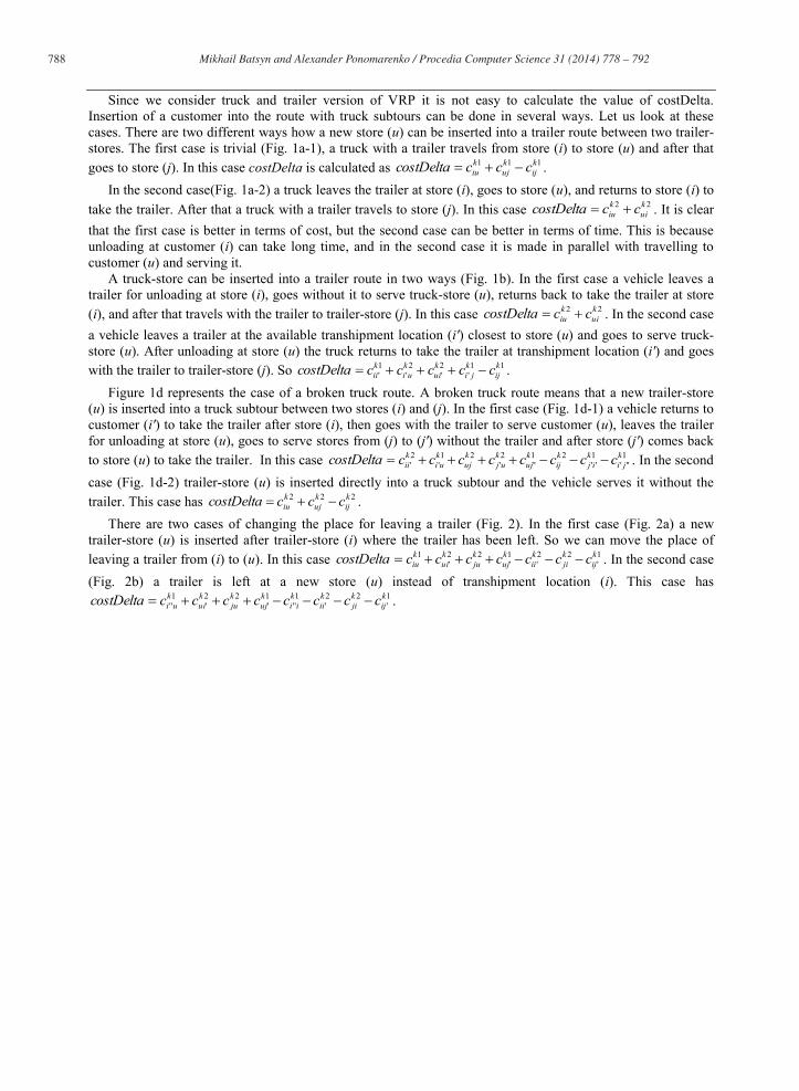
Since we consider truck and trailer version of VRP it is not easy to calculate the value of costDelta. Insertion of a customer into the route with truck subtours can be done in several ways. Let us look at these cases. There are two different ways how a new store (u) can be inserted into a trailer route between two trailer-stores. The first case is trivial (Fig. 1a-1), a truck with a trailer travels from store (i) to store (u) and after that goes to store (j). In this case costDelta is calculated as 111 k
ijkuj
kiu ccccostDelta .
In the second case(Fig. 1a-2) a truck leaves the trailer at store (i), goes to store (u), and returns to store (i) to take the trailer. After that a truck with a trailer travels to store (j). In this case 22 k
uikiu cccostDelta . It is clear
that the first case is better in terms of cost, but the second case can be better in terms of time. This is because unloading at customer (i) can take long time, and in the second case it is made in parallel with travelling to customer (u) and serving it.
A truck-store can be inserted into a trailer route in two ways (Fig. 1b). In the first case a vehicle leaves a trailer for unloading at store (i), goes without it to serve truck-store (u), returns back to take the trailer at store (i), and after that travels with the trailer to trailer-store (j). In this case 22 k
uikiu cccostDelta . In the second case
a vehicle leaves a trailer at the available transhipment location (i') closest to store (u) and goes to serve truck-store (u). After unloading at store (u) the truck returns to take the trailer at transhipment location (i') and goes with the trailer to trailer-store (j). So 11
'2'
2'
1'
kij
kji
kui
kui
kii ccccccostDelta .
Figure 1d represents the case of a broken truck route. A broken truck route means that a new trailer-store (u) is inserted into a truck subtour between two stores (i) and (j). In the first case (Fig. 1d-1) a vehicle returns to customer (i') to take the trailer after store (i), then goes with the trailer to serve customer (u), leaves the trailer for unloading at store (u), goes to serve stores from (j) to (j') without the trailer and after store (j') comes back to store (u) to take the trailer. In this case 1
'''1''
21''
2'
21'
2'
kji
kij
kij
kuj
kuj
kuj
kui
kii cccccccccostDelta . In the second
case (Fig. 1d-2) trailer-store (u) is inserted directly into a truck subtour and the vehicle serves it without the trailer. This case has 222 k
ijkuj
kiu ccccostDelta .
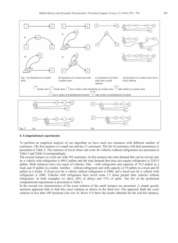
There are two cases of changing the place for leaving a trailer (Fig. 2). In the first case (Fig. 2a) a new trailer-store (u) is inserted after trailer-store (i) where the trailer has been left. So we can move the place of leaving a trailer from (i) to (u). In this case 1
'22
'1'
22'
1 kij
kji
kii
kuj
kju
kui
kiu ccccccccostDelta . In the second case
(Fig. 2b) a trailer is left at a new store (u) instead of transhipment location (i). This case has 1'
22'
1''
1'
22'
1''
kij
kji
kii
kii
kuj
kju
kui
kui cccccccccostDelta .
789 Mikhail Batsyn and Alexander Ponomarenko / Procedia Computer Science 31 ( 2014 ) 778 – 792
Fig. 1 (a) Insertion of a trailer-store
(b) Insertion of a truck-store into a trailer route
(c) Insertion of a truck-store into a truck subtour
(d) Insertion of a trailer-store into a truck subtour
trailer-store truck-store leave trailer with unloading at a trailer-store take trailer at a trailer-store
leave trailer at transhipment location take trailer at transhipment location
Fig. 2 (a) (b) 4. Computational experiments To perform an empirical analysis of our algorithm we have used two instances with different number of customers. The first instance is a small one and has 11 customers. The list of customers with their parameters is presented in Table 2. The matrices of travel times and costs for vehicles without refrigerators are presented in Table 3 and Table 4 correspondingly. The second instance is a real one with 292 customers. In this instance the total demand that can be served only by a vehicle with refrigerator is 490.5 pallets and the total demand that does not require refrigerator is 2293.5 pallets. Both instances have two types of vehicles. One – with refrigerator and capacity of 19.5 pallets in a truck and 19 pallets in a trailer. Another – without refrigerator and with capacity of 19 pallets in a truck and 20 pallets in a trailer. A fixed cost for a vehicle without refrigerator is 2000, and a fixed cost for a vehicle with refrigerator is 2600. Vehicles with refrigerator have travel costs 1.5 times greater than vehicles without refrigerator. In both examples we allow 20% of delays and 15% of splits. The list of the performed computational experiments is presented in Table 1. In the second row characteristics of the exact solution of the small instance are presented. A simple greedy insertion approach fails to find this exact solution as shown in the third row. Our approach finds the exact solution in less than 100 iterations (see row 4). Rows 5-9 show the results obtained for the real-life instance.
790 Mikhail Batsyn and Alexander Ponomarenko / Procedia Computer Science 31 ( 2014 ) 778 – 792
The suggested approach finds a solution with 20% lower cost than the simple greedy one. It spends about one hour to make 100k iterations to get such a solution. It is not reasonable to make more than 100k iterations because the solution improves insignificantly for 1000k iterations. Table 1. Computational experiments.
Instance Total cost, rub Distance, km km/pallets Number of vehicles
without ref.
Number of vehicles with ref.
Percent of time window
violations
Percent of splits
Small test - exact solution
70035 3720 35.7692 2 4 18 0
Small test - simple greedy
102464 4342 51.75 4 5 18 0
Small test - our algorithm - 100 iterations
70035 3720 35.7692 2 4 18 0
Real test - simple greedy 1217452 64907 24.7223 61 51 20 11 Real test - our algorithm - 1000 iterations
984599 52780 18.9583 50 39 17 11
Real test - our algorithm - 10k iterations
974712 52325 18.7949 49 39 18 8
Real test - our algorithm - 100k iterations
966671 51718 18.5769 49 39 18 9
Real test - our algorithm - 1000k iterations
963242 51324 18.3224 48 39 19 12
Table 2. Customers.
Customer Ref. demand No ref. demand
Soft time widow begin
Soft time window end
Open time (hard time window)
Close time (hard time window)
Is truck-store
1 0 10.5 15:00 16:00 10:00 21:00 Y 2 0 10 11:30 12:30 10:00 22:30 Y 3 1 4.5 15:00 16:00 10:00 21:30 Y 4 0 9.5 10:00 11:00 9:30 21:00 N 5 2 7 10:00 11:00 10:00 22:00 N 6 1.5 7 10:00 11:00 10:00 21:30 N 7 0 9 16:00 17:00 10:00 21:00 N 8 6.5 9.5 11:00 12:00 10:00 22:00 Y 9 2 7 12:30 13:30 10:00 22:00 Y
10 0 7.5 17:30 18:30 10:00 22:00 Y 11 2.5 7 18:00 19:00 9:30 20:00 N
The authors are supported by LATNA Laboratory, NRU HSE, RF government grant, ag. 11.G34.31.0057.
References
[1] Caramia M., Guerriero F., 2010a. A heuristic approach for the truck and trailer routing problem. Journal of the Operational Research Society 61, p. 1168–1180.
[2] Caramia M., Guerriero F., 2010b. A milk collection problem with incompatibility constraints. Interfaces 40(2), p. 130–143. [3] Chao, I. M., 2002. A tabu search method for the truck and trailer routing problem. Computers & Operations Research 29(1), p. 33–51. [4] Drexl, M., 2011. Branch-and-Price and Heuristic Column Generation for the Generalized Truck-and-Trailer Routing Problem. Journal
of Quantitative Methods for Economics and Business Administration 12(1), p. 5-38. [5] Hoff, A., 2006. Heuristics for rich vehicle routing problems. Ph.D. Thesis. Molde University College. [6] Hoff, A., Lokketangen A., 2007. A tabu search approach for milk collection in western Norway using trucks and trailers. The sixth
triennial symposium on transportation analysis TRISTAN VI. Phuket, Tailand. [7] Lin, S.-W., Yu, V. F., Chou, S.-Y., 2009. Solving the truck and trailer routing problem based on a simulated annealing heuristic.
Computers & Operations Research 36(5), p. 1683–1492. [8] Lin, S.-W., Yu, V. F., Chou, S.-Y., 2010. A note on the truck and trailer routing problem. Expert Systems with Applications 37(1), p.
899–903. [9] Lin, S.-W., Yu, V. F., Lu, C.-C., 2011. A simulated annealing heuristic for the truck and trailer routing problem with time windows.
Expert Systems with Applications 38, p. 15244-15252. [10] Scheuerer, S., 2006. A tabu search heuristic for the truck and trailer routing problem. Computers & Operations Research 33, p. 894–
909. [11] Semet, F., Taillard, E., 1993. Solving real-life vehicle routing problems efficiently using tabu search. Annals of Operations Research
41, p. 469–488. [12] Semet, F., 1995. A two-phase algorithm for the partial accessibility constrained vehicle routing problem. Annals of Operations
Research 61, p. 45–65.
792 Mikhail Batsyn and Alexander Ponomarenko / Procedia Computer Science 31 ( 2014 ) 778 – 792
[13] Solomon, M. M., 1987. Algorithms for the vehicle routing and scheduling problem with time window constraints. Operations Research 35, p. 254–265.
[14] Villegas, J. G., Prins, C., Prodhon, C., Medaglia, A. L., Velasco, N., 2011a. A GRASP with evolutionary path relinking for the truck and trailer routing problem. Computers & Operations Research 38(9), p. 1319-1334.
[15] Villegas, J. G., Prins, C., Prodhon, C., Medaglia, A. L., Velasco, N., 2011b. Heuristic column generation for the truck and trailer routing problem. International Conference on Industrial Engineering and Systems Management IESM’2011. Metz, France.