21
Heuristic Search: A* 1 CPSC 322 – Search 4 January 19, 2011 Textbook §3.6 Taught by: Vasanth
Heuristic Search: A*
1
CPSC 322 – Search 4January 19, 2011
Textbook §3.6Taught by: Vasanth
Lecture Overview
• Recap
• Search heuristics: admissibility and examples
• Recap of BestFS
• Heuristic search: A*
2
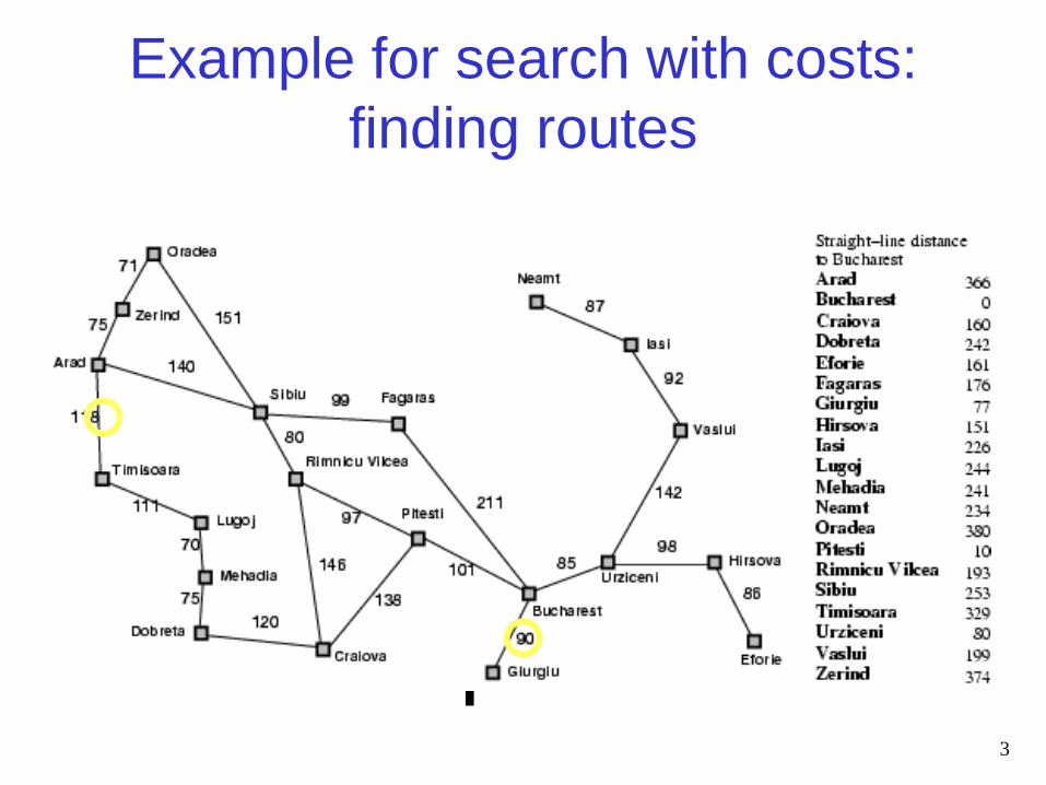
Example for search with costs: finding routes
3
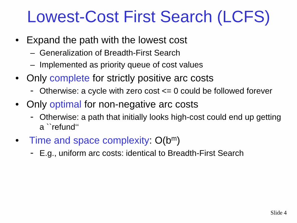
Lowest-Cost First Search (LCFS)• Expand the path with the lowest cost
– Generalization of Breadth-First Search– Implemented as priority queue of cost values
• Only complete for strictly positive arc costs- Otherwise: a cycle with zero cost <= 0 could be followed forever
• Only optimal for non-negative arc costs- Otherwise: a path that initially looks high-cost could end up getting
a ``refund‘‘
• Time and space complexity: O(bm)- E.g., uniform arc costs: identical to Breadth-First Search
Slide 4
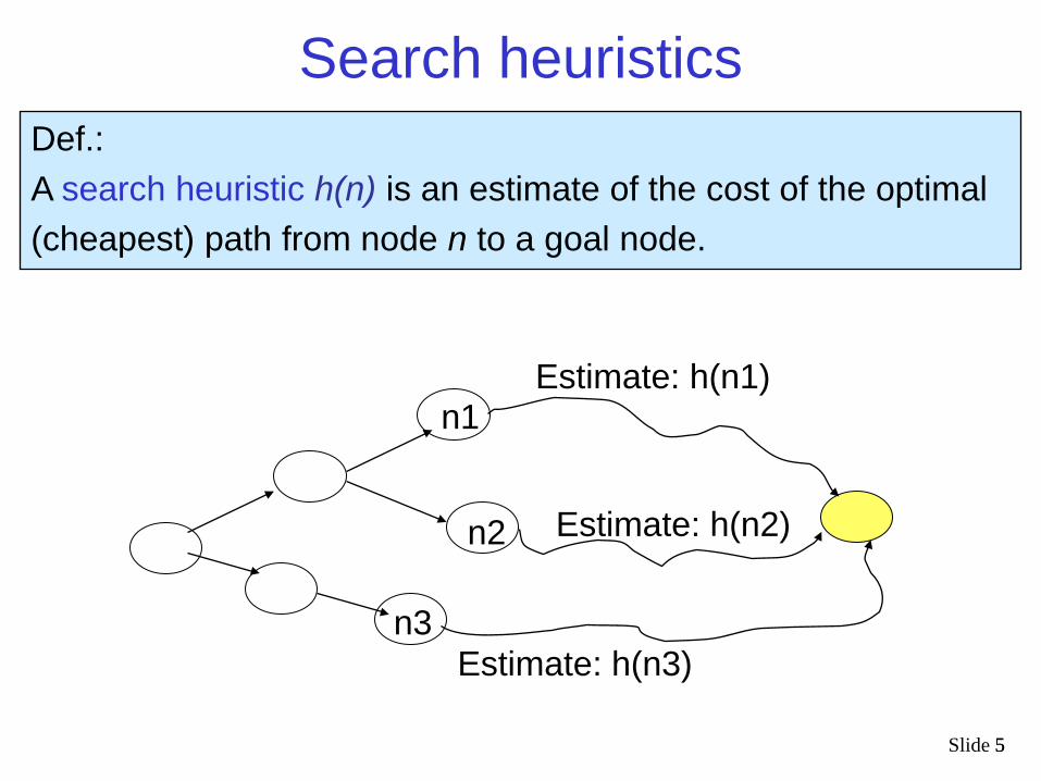
Search heuristics
Slide 5
Def.: A search heuristic h(n) is an estimate of the cost of the optimal (cheapest) path from node n to a goal node.
Estimate: h(n1)
5
Estimate: h(n2)
Estimate: h(n3)n3
n2
n1
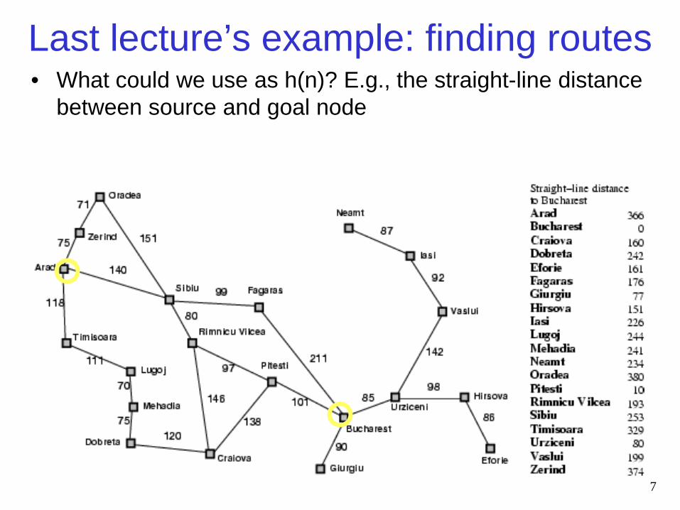
Last lecture’s example: finding routes
7
• What could we use as h(n)? E.g., the straight-line distance between source and goal node
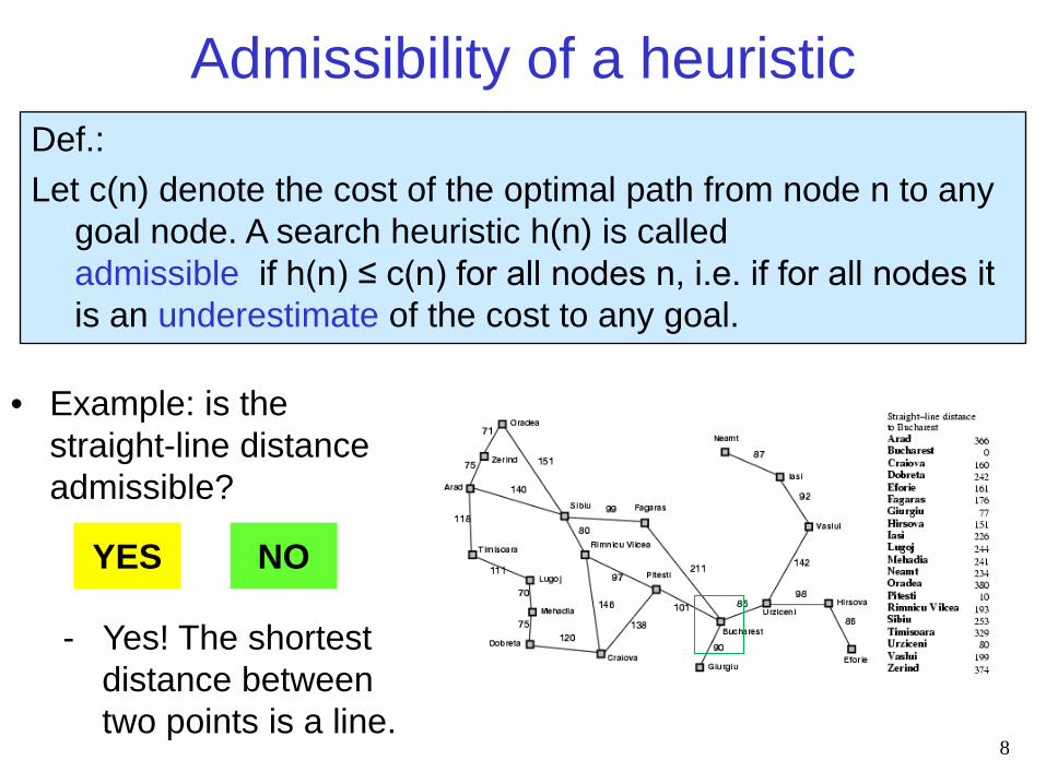
Admissibility of a heuristic
8
Def.: Let c(n) denote the cost of the optimal path from node n to any
goal node. A search heuristic h(n) is called admissible if h(n) ≤ c(n) for all nodes n, i.e. if for all nodes it is an underestimate of the cost to any goal.
• Example: is the straight-line distance admissible?
- Yes! The shortest distance between two points is a line.
YES NO
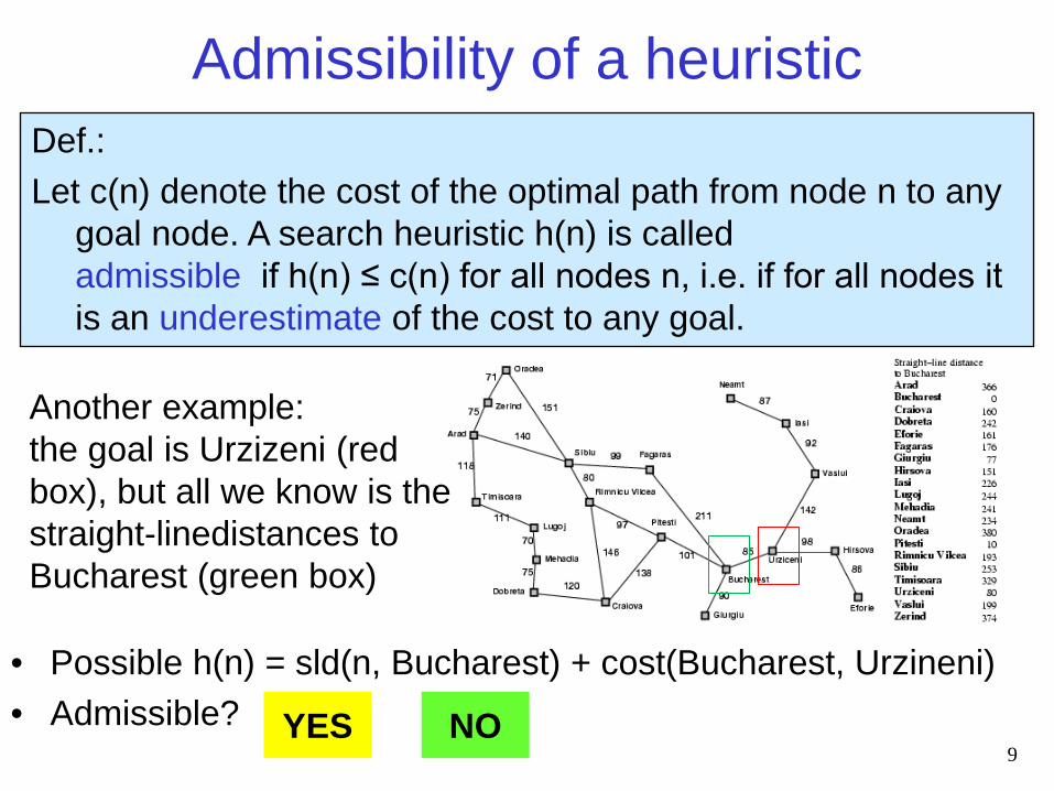
Admissibility of a heuristic
9
Def.: Let c(n) denote the cost of the optimal path from node n to any
goal node. A search heuristic h(n) is called admissible if h(n) ≤ c(n) for all nodes n, i.e. if for all nodes it is an underestimate of the cost to any goal.
Another example: the goal is Urzizeni (red box), but all we know is the straight-linedistances to Bucharest (green box)
YES NO
• Possible h(n) = sld(n, Bucharest) + cost(Bucharest, Urzineni)• Admissible?
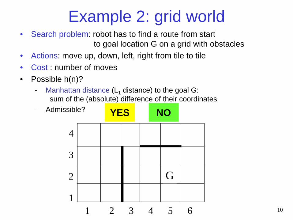
Example 2: grid world• Search problem: robot has to find a route from start
to goal location G on a grid with obstacles• Actions: move up, down, left, right from tile to tile• Cost : number of moves• Possible h(n)?
- Manhattan distance (L1 distance) to the goal G: sum of the (absolute) difference of their coordinates
- Admissible?
101 2 3 4 5 6
G
4
3
2
1
YES NO
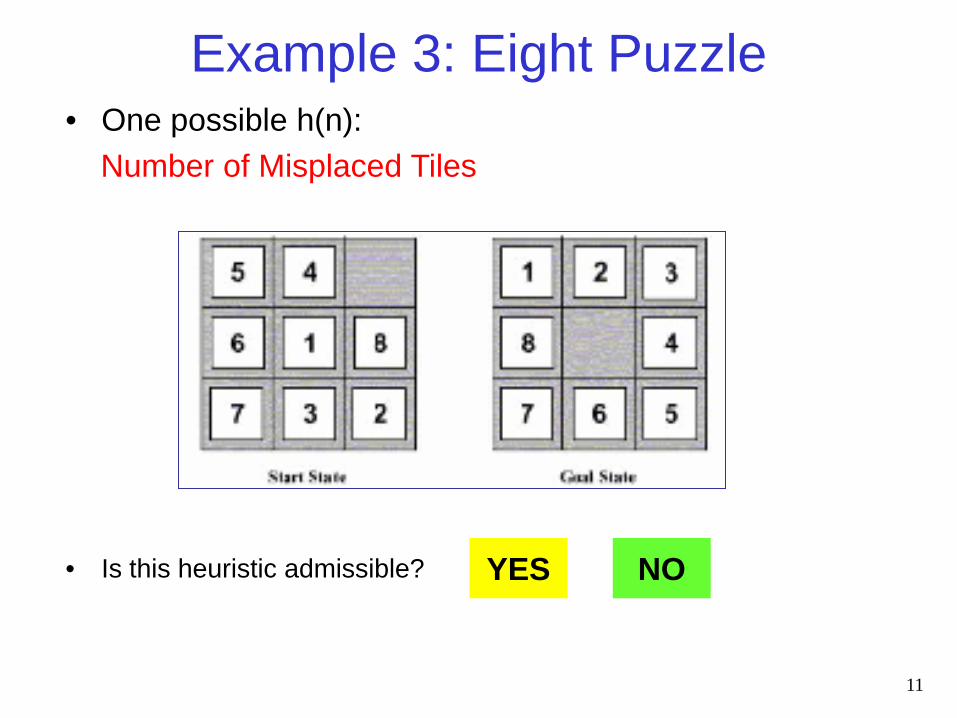
Example 3: Eight Puzzle
11
• One possible h(n):Number of Misplaced Tiles
YES NO• Is this heuristic admissible?
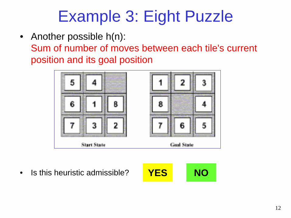
Example 3: Eight Puzzle
12
• Another possible h(n): Sum of number of moves between each tile's current position and its goal position
YES NO• Is this heuristic admissible?
How to Construct an Admissible Heuristic
13
• Identify relaxed version of the problem: - where one or more constraints have been dropped- problem with fewer restrictions on the actions
• Grid world: the agent can move through walls• Driver: the agent can move straight• 8 puzzle:
- “number of misplaced tiles”:tiles can move everywhere and occupy same spot as others
- “sum of moves between current and goal position”:tiles can occupy same spot as others
• Why does this lead to an admissible heuristic?- The problem only gets easier!
Lecture Overview
• Recap
• Search heuristics: admissibility and examples
• Recap of BestFS
• Heuristic search: A*
14
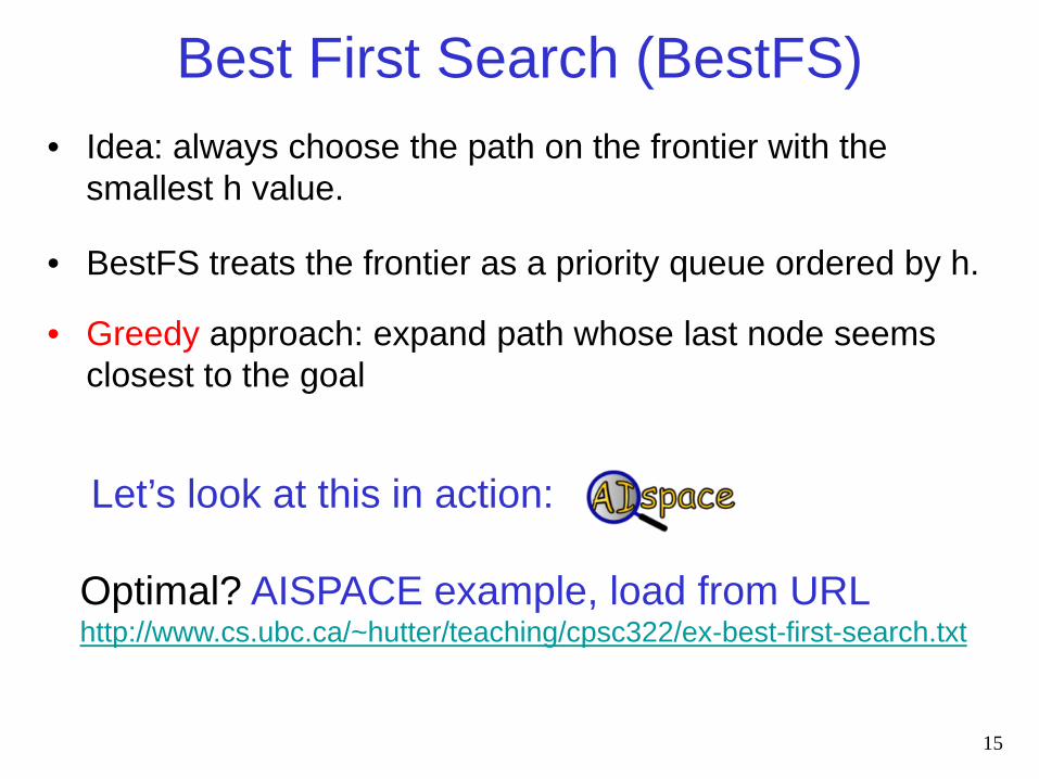
• Idea: always choose the path on the frontier with the smallest h value.
• BestFS treats the frontier as a priority queue ordered by h.
• Greedy approach: expand path whose last node seems closest to the goal
Best First Search (BestFS)
15
Let’s look at this in action:
Optimal? AISPACE example, load from URLhttp://www.cs.ubc.ca/~hutter/teaching/cpsc322/ex-best-first-search.txt
Lecture Overview
• Recap
• Search heuristics: admissibility and examples
• Recap of BestFS
• Heuristic search: A*
17
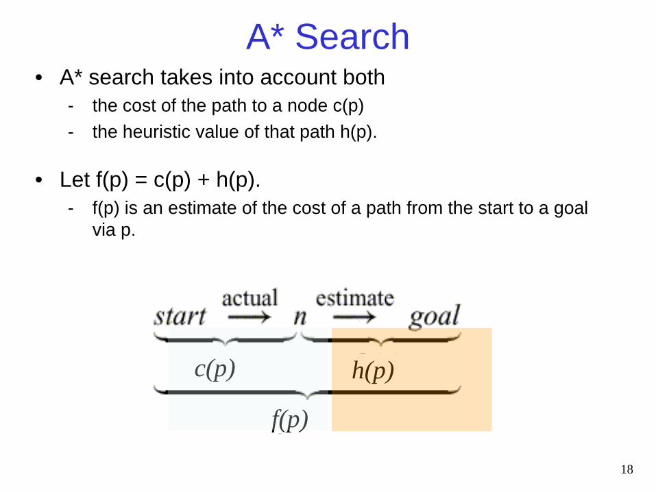
• A* search takes into account both - the cost of the path to a node c(p) - the heuristic value of that path h(p).
• Let f(p) = c(p) + h(p). - f(p) is an estimate of the cost of a path from the start to a goal
via p.
A* Search
c(p) h(p)
f(p)
18
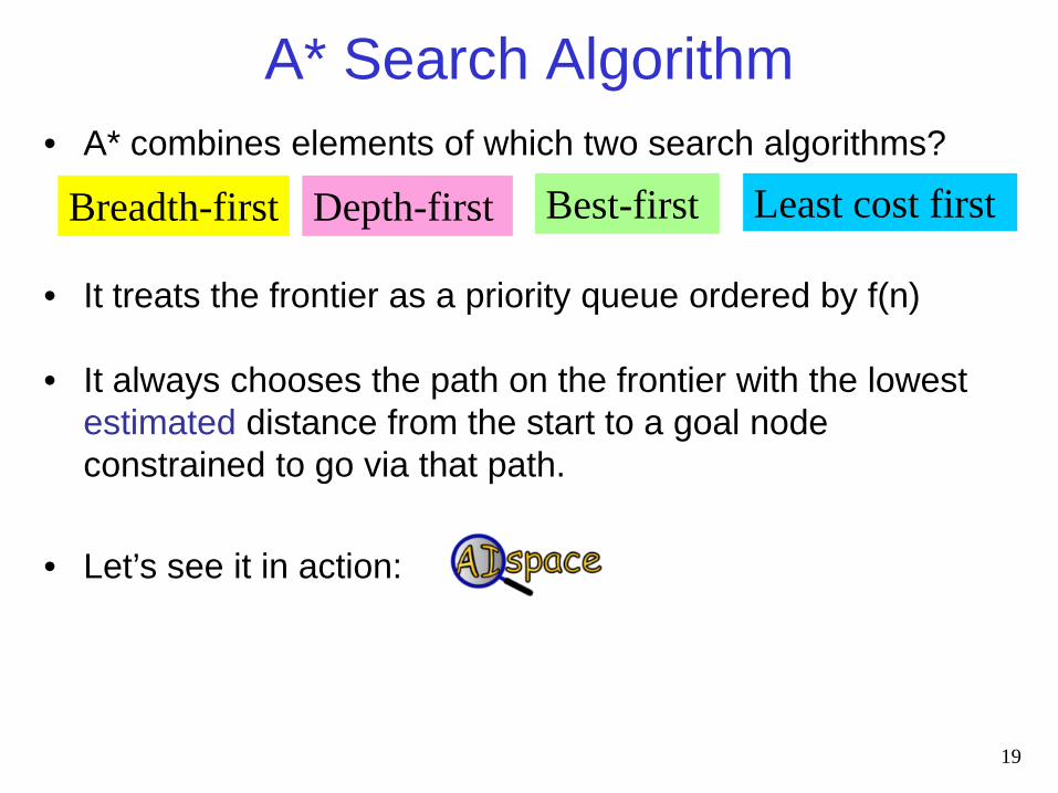
• A* combines elements of which two search algorithms?
• It treats the frontier as a priority queue ordered by f(n)
• It always chooses the path on the frontier with the lowest estimated distance from the start to a goal node constrained to go via that path.
• Let’s see it in action:
A* Search Algorithm
19
Least cost firstBreadth-first Best-firstDepth-first

A* in Infinite Mario Bros
20
http://www.youtube.com/watch?v=DlkMs4ZHHr8
Analysis of A*
21
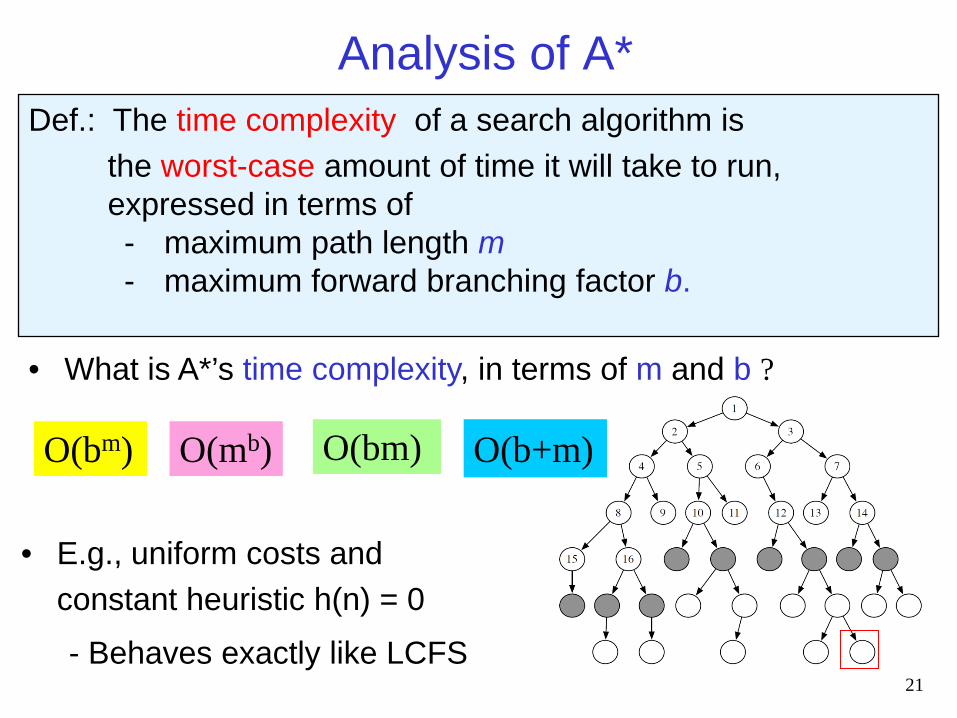
• What is A*’s time complexity, in terms of m and b ?
• E.g., uniform costs and constant heuristic h(n) = 0
- Behaves exactly like LCFS
Def.: The time complexity of a search algorithm is the worst-case amount of time it will take to run, expressed in terms of - maximum path length m- maximum forward branching factor b.
O(b+m)O(bm) O(bm)O(mb)
• A* is complete (finds a solution, if one exists) and optimal (finds the optimal path to a goal) if:- the branching factor is finite- arc costs are > 0 - h(n) is admissible -> an underestimate of the length of the
shortest path from n to a goal node.
• This property of A* is called admissibility of A*
A* completeness and optimality
23
• Construct heuristic functions for specific search problems Define/read/write/trace/debug different search algorithms
- With/without cost- Informed/Uninformed
• Formally prove A* optimality (continued next class)
24
Learning Goals for today’s class


![Informed [Heuristic] Search - University of Delawaredecker/courses/681s07/pdfs/04-Heuristic...Informed [Heuristic] Search Heuristic: “A rule of thumb, simplification, or educated](https://static.documents.pub/doc/80x56/5aa1e13c7f8b9a84398c48b6/informed-heuristic-search-university-of-delaware-deckercourses681s07pdfs04-heuristicinformed.jpg)


