AC 2011-1013: HEV GREEN MOBILITY LABORATORY

Mark G. Thompson, Kettering University

Dr. Mark G. Thompson is a Professor of Electrical Engineering at Kettering University. He teaches in theareas of electronic design and automotive electronic control. He has been involved in many alternativeenergy and alternative fueled vehicle research projects including development of power electronic andcontrol interfaces for photovoltaic arrays, hybrid electric vehicles and fuel cell vehicles.

Craig J. Hoff, Kettering University

Dr. Craig J. Hoff is a Professor of Mechanical Engineering at Kettering University. He teaches in the areasof thermal design, mechanical design, and automotive engineering. His research focuses on sustainablemobility technologies including alternative fuels, fuel cells and hybrid electric vehicles. He is activelyinvolved in the Society of Automotive Engineers and is the faculty advisor for Kettering’s Formula SAErace team. Dr. Hoff is a registered Professional Engineer in the State of Michigan.

James Gover, Kettering University

Dr. Gover holds a Ph.D. in nuclear engineering and an MS in electrical engineering from the Universityof New Mexico. He is retired from Sandia National Laboratories and has been Professor of electrical en-gineering at Kettering University for 13 years. His honors include selection as IEEE Fellow and recipientof IEEE Citation of Honor. He has served IEEE in numerous conference positions and as CongressionalFellow and Competitiveness Fellow.

Allan R Taylor, Kettering University

Allan Taylor attained his BSEE degree from Kettering University in Spring 2009 with honors (MagnaCum-Laude) and is a member of Eta Kappa Nu electrical engineering honor society. Allan is currentlyworking on his Master’s in Engineering (with concentration in ECE) and has been awarded a full schol-arship and assistantship at Kettering University. Allan has had extensive experience with HEV relatedtopics in his undergraduate and graduate coursework and has volunteered time as a Power Electronics& Electrical Drive Train engineer for Kettering’s fuel cell formula race car team for which he has beendeveloping computer controls system models. Allan has been selecting equipment for the Green MobilityLaboratory and aiding the design of experiments and simulations for the lab.

Michelle R. Pomeroy, Kettering University

Michelle Pomeroy attained her BSEE from Kettering University in June 2002 receiving the PresidentsMedal given to only 2% of each graduating class for professionalism in the workplace, community in-volvement and participation in professional societies. Since graduation Michelle has received her MS inEngineering Management from Oakland University, a Masters Certificate from Villanova University inProject Management and is currently pursuing a Master’s of Science in Engineering with a concentrationin Electrical and Computer Engineering from Kettering University. She worked for Delphi from 1997 to2009 in various positions, most recently focusing in applications engineering and project management.Michelle is doing project management support activities and assisting with software development for theGreen Mobility Laboratory.

Kevin (Hua) Bai, Kettering Univ

Kevin Bai received B S and PHD degree in Department of Electrical Engineering of Tsinghua University.,Beijing, China in 2002 and 2007, respectively. He was a post-doc fellow and research scientist in Univ ofMichigan-Dearborn, USA, in 2007 and 2009, respectively. Now he is an assistant professor in Departmentof Electrical and Compurter Engineering, Kettering University, MI, USA. His research interest is thedynamic processes and transient pulsed power phenomena of power electronic devices, including variablefrequency motor drive system, high voltage and high power DC/DC converter, renewable energy andhybrid electric vehicles.

c©American Society for Engineering Education, 2011

Hybrid Electric Vehicle “Green Mobility” Laboratory

Abstract

The implementation of a Hybrid Electric Vehicle (HEV) Green Mobility Laboratory to aid in the

development of an innovative and flexible educational program in transportation electrification is

described. The high level objectives of the program are: (1) to provide unique and timely

educational opportunities for undergraduate students as a basis for the advancement of

transportation electrification, and (2) to provide research facilities and opportunities for graduate

students and faculty in the Department of Electrical and Computer Engineering (ECE) that will

establish the future direction of electric transportation for the country and the world.

The Green Mobility Laboratory consists of three open-bench, hybrid electric vehicle drive train

control, simulation, and data acquisition systems. The hybrid drive train components on each

bench include a DC power supply / battery pack simulator, 3-phase DC-AC Pulse Width

Modulated (PWM) controlled inverter motor drive, 5 kW permanent magnet synchronous motor

(PMSM), and Eddy current dynamometer load. Power and waveform measurements are made

with a Precision Power Analyzer and PC based data acquisition system. The drive train

components and instrumentation are integrated in a flexible control and simulation laboratory for

utilization in several curricular and research activities. Two new courses utilizing the Green

Mobility Laboratory are being developed for the ECE curriculum. Details of the laboratory

implementation and utilization within the ECE curriculum focusing on transportation

electrification are described.

Introduction

In the United States, national and state transportation policy experts consider electric and hybrid

electric vehicles (HEVs) to be a key technology for reducing dependence on oil imports and for

lowering the production of greenhouse gas emissions generated by the transportation sector. The

Institute of Electrical and Electronic Engineers (IEEE) Energy Policy Committee emphasize the

importance of HEV power trains in its recommendations to Congress. HEV power trains are

more complex and operate much differently than conventional vehicle power trains in many

respects. Thus, well established and existing conventional design techniques, control algorithms,

and testing methods are not directly applicable to HEVs. Education of a new generation of

engineers with interdisciplinary knowledge capable of meeting the challenges presented by the

electrification of the transportation industry must serve as a central component in a strategy to

gain U.S. energy independence. To this end, the implementation of a Hybrid Electric Vehicle

Green Mobility Laboratory to aid in the development of an innovative and flexible educational

program in transportation electrification is described in this paper. The high level objectives of

the program are: (1) to provide unique and timely educational opportunities to undergraduate

students as a basis for the advancement of transportation electrification, and (2) to provide

research facilities and opportunities for graduate students and faculty in the Department of

Electrical and Computer Engineering (ECE) that will establish the future direction of electric

transportation for the country and the world.

This program was initiated in response to a definition of hybrid electric industry education needs

identified by the Michigan Academy for Green Mobility and is supported by the United States

Department of Energy with funds provided by the American Recovery and Reinvestment Act.

Background & Motivation

To help reduce emissions from internal combustion engines, increase fuel economy, realign

transportation energy needs toward domestic resources, and generally assist the U.S. automobile

industry in meeting the economic and technical challenges of a new era of electric vehicles,

engineering programs must provide transportation electrification (“green mobility”) educational

opportunities to undergraduate and graduate students. The Michigan Academy for Green

Mobility was established to provide an ongoing government-industrial-academic partnership

with a goal to support the transformation of the domestic automotive industry in the State of

Michigan. The education needs, desired courses, and laboratory requirements to support this

transformation were determined through active participation by more than thirty OEM and

supplier companies working in the hybrid vehicle sector and from more than ten regional

colleges and universities.

A meaningful educational program in transportation electrification must involve an integrated

and interdisciplinary curriculum that includes; energy storage systems, power electronics,

electric drives, digital electronic control, local area network communications, and the mechanics

of automotive power trains. The Michigan Academy for Green Mobility determined, as part of

this effort, that Michigan universities should develop undergraduate and graduate education

programs to fulfill the identified needs. A preponderance of these new educational needs were in

electrical engineering. It was concluded that industry supportive undergraduate education

requirements could be met at Kettering University by: (1) existing courses (from the standard

Electrical and Computer Engineering (ECE) and Mechanical Engineering curricula), (2)

development of two new ECE courses that fulfill specialized needs identified by industry, and

(3) utilizing battery controls courses being developed and taught at the University of Michigan.

To properly teach this curriculum with equal emphasis on theory, simulation and hands-on

laboratory experiences, would require the cross-disciplinary (electrical engineering, computer

engineering, and mechanical engineering) development of an integrated hybrid vehicle power

electronics laboratory. The HEV Green Mobility Laboratory is the outcome of this effort.

The Green Mobility Laboratory has been designed to support hands-on undergraduate student

experiments, faculty demonstrations, independent studies, and graduate student research projects.

The laboratory opened for the Fall 2010 academic semester and was utilized in the first new

course, Design, Simulation, and Control of Power Electronic Circuits for Electric Drive Trains

for several demonstration exercises. The first offering of this course was via a “special topics”

class with a limited enrollment of 5 students. Laboratory development continued through the

Winter 2011 semester with refinements to the system control software, hardware, and user

interface to make it easier and safer for undergraduate students to perform hands-on experiments.

Examples of the control interface and a sample laboratory exercise are presented in this paper.

Starting with the Spring 2011 academic term, the Green Mobility Laboratory should be fully

functional for undergraduate laboratory experiments associated with the second new course,

Semiconductor Switching: Electrical and Thermal Effects. For the 2011-2012 academic year, the

Green Mobility Laboratory will be utilized in both new courses and two existing courses (Power

Electronics and Applications; and Hybrid Electric Vehicle Propulsion) with a projected total

student enrollment of 75 students. The laboratory is currently ready for industry sponsored

graduate student research projects.

Laboratory Hardware Description

The Green Mobility Laboratory consists of three open-bench, hybrid electric vehicle drive train

control, simulation, and data acquisition systems. The hybrid drive train components on each

bench include:

• Programmable DC power supply / battery pack simulator

• 3-phase DC-AC Pulse Width Modulated (PWM) controlled inverter motor drive and cooling

loop controller

• 5 kW permanent magnet synchronous motor (PMSM)

• Eddy current dynamometer load / vehicle dynamics simulator

Figure 1. Green Mobility Laboratory station (one of three)

Power and waveform measurements are made with a Precision Power Analyzer and PC based

data acquisition system. The drive train components and instrumentation are integrated with a

flexible control and simulation software, developed at Kettering University and written with

National Instruments LabVIEW 8.6. The Graphical User Interface (GUI) communicates with

each device either through serial communication (RS-232) or through an Ethernet connection.

As depicted in the system block diagram of Figure 2, electrical and mechanical power

measurements are made with a Yokogawa Power Analyzer. The DC electrical output power of

the power supply, 3-phase AC electrical power of the inverter, and the mechanical output power

of the motor are measured. Thus, efficiencies for the inverter and motor can be calculated under

any operating condition.

Figure 2. Green Mobility Lab system-block-diagram

Also shown in the system block diagram, the 3-phase inverter is water-cooled. Temperature and

flow sensors have been included in the inverter coolant loop to allow thermodynamic calculation

of heat loss. This calculation can be experimentally compared to the measured inverter electrical

power loss from the power analyzer.

The coolant loop is controlled by a National Instruments Compact Reconfigurable I/O (cRIO).

The cRIO communicates with the host PC’s software GUI to generate 3 PWM signals. These

PWM signals drive three DC/DC step-down converters to generate three variable DC voltages

from a single fixed 24 V DC power supply (Figures 3 and 4). Thus, fan speed, pump speed, and

12 V inverter logic can be powered and controlled through software.

Figure 3. Coolant loop controller block diagram

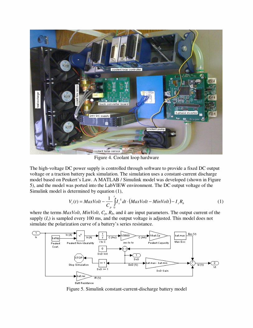
Figure 4. Coolant loop hardware

The high-voltage DC power supply is controlled through software to provide a fixed DC output

voltage or a traction battery pack simulation. The simulation uses a constant-current discharge

model based on Peukert’s Law. A MATLAB / Simulink model was developed (shown in Figure

5), and the model was ported into the LabVIEW environment. The DC output voltage of the

Simulink model is determined by equation (1),

( )bs

tk

s

p

t RIMinVoltMaxVoltdtIC

MaxVolttV −−⋅−= ∫0

1)( (1)

where the terms MaxVolt, MinVolt, Cp, Rb, and k are input parameters. The output current of the

supply (Is) is sampled every 100 ms, and the output voltage is adjusted. This model does not

simulate the polarization curve of a battery’s series resistance.

Figure 5. Simulink constant-current-discharge battery model

The GUI software panel for the programmable DC power supply / battery pack simulator is

shown in Figure 6. Through the software panel, students can enter the modeling parameters of

the battery, reset the Depth of Discharge (DoD) counter, and toggle the supply output to simulate

a wide variety of HEV traction battery packs and conditions.

Figure 6. Software panel for DC power supply / battery pack simulator

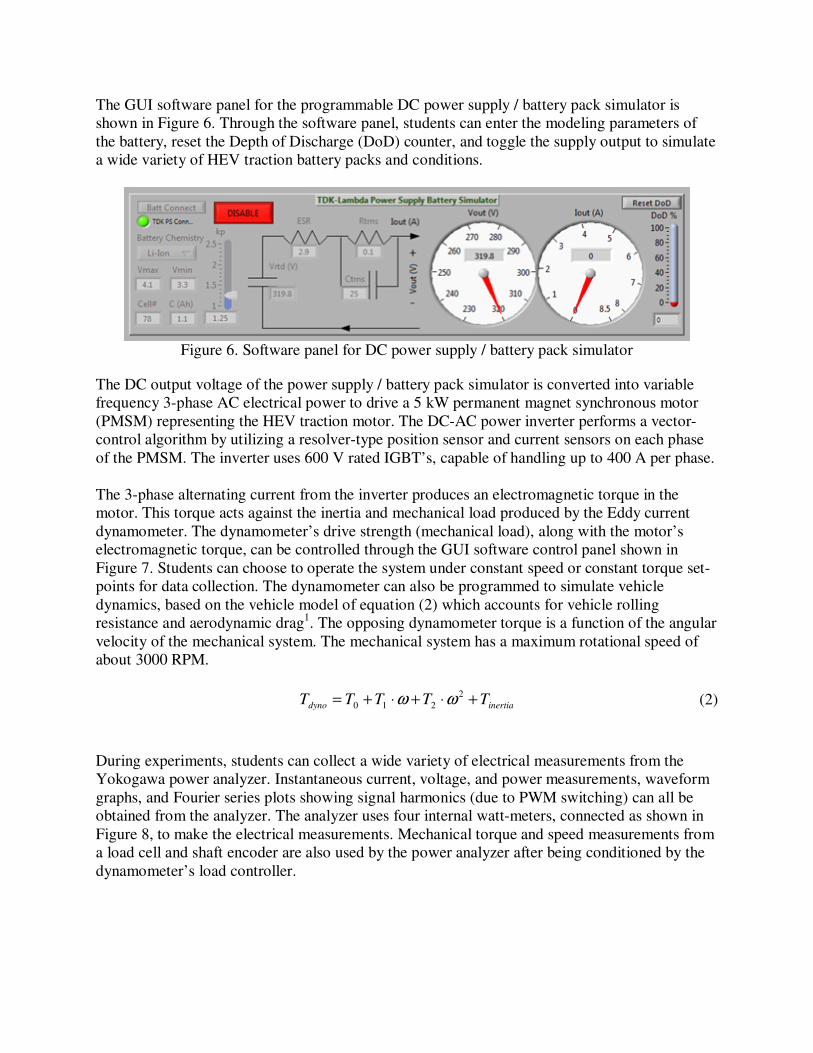
The DC output voltage of the power supply / battery pack simulator is converted into variable

frequency 3-phase AC electrical power to drive a 5 kW permanent magnet synchronous motor

(PMSM) representing the HEV traction motor. The DC-AC power inverter performs a vector-

control algorithm by utilizing a resolver-type position sensor and current sensors on each phase

of the PMSM. The inverter uses 600 V rated IGBT’s, capable of handling up to 400 A per phase.

The 3-phase alternating current from the inverter produces an electromagnetic torque in the

motor. This torque acts against the inertia and mechanical load produced by the Eddy current

dynamometer. The dynamometer’s drive strength (mechanical load), along with the motor’s

electromagnetic torque, can be controlled through the GUI software control panel shown in

Figure 7. Students can choose to operate the system under constant speed or constant torque set-

points for data collection. The dynamometer can also be programmed to simulate vehicle

dynamics, based on the vehicle model of equation (2) which accounts for vehicle rolling

resistance and aerodynamic drag1. The opposing dynamometer torque is a function of the angular

velocity of the mechanical system. The mechanical system has a maximum rotational speed of

about 3000 RPM.

inertiadyno TTTTT +⋅+⋅+=2

210 ωω (2)

During experiments, students can collect a wide variety of electrical measurements from the

Yokogawa power analyzer. Instantaneous current, voltage, and power measurements, waveform

graphs, and Fourier series plots showing signal harmonics (due to PWM switching) can all be

obtained from the analyzer. The analyzer uses four internal watt-meters, connected as shown in

Figure 8, to make the electrical measurements. Mechanical torque and speed measurements from

a load cell and shaft encoder are also used by the power analyzer after being conditioned by the

dynamometer’s load controller.

Figure 7. Inverter and dynamometer software control panels

Figure 8. Yokogawa electrical power measurement connections

New Electrical Engineering Courses Utilizing the Green Mobility Laboratory

Two new courses utilizing the Green Mobility Laboratory are being developed for the ECE

curriculum 1) Design, Simulation, and Control of Power Electronic Circuits for Electric Drive

Trains, and 2) Semiconductor Switching: Electrical and Thermal Effects. Outlines of the course

descriptions and laboratory time allocation for each course within the ECE curriculum are

presented in Figures 9 and 10.

New ECE Course Outline (1): Design, Simulation, and Control of Power Electronic Circuits for

Electric Drive Trains

• Introduction to the application and roles of power electronics in EV/HEV/PHEV drive trains.

• Analytical circuit design, simulation using Multi-Sim, control and testing with limitation for

use in EV/HEV/PHEV systems highlighted

• State variable models of traditional uni-directional, IGBT switched, pulse width

modulated (PWM), DC-DC converters

• State variable models of bi-directional, isolated, PWM, DC-DC converters

• State space models of IGBT-switched DC-AC inverters under different PWM

conditions

• Electromagnetic Interference (EMI) in electric drive trains.

• Review of commercially available power IGBT devices, power modules and testing methods.

Figure 9. Design, Simulation, and Control of Power Electronic Circuits for Electric Drive

Trains: Lecture and laboratory time allocation

New ECE Course Outline (2): Semiconductor Switching: Electrical and Thermal Effects

• Relationship between IGBT electrical heating, cooling system design and IGBT electrical

behavior

• Introduction to power semiconductors, semiconductor internals & analytical models

• IGBT physical & electrical characteristics and IGBT parasitic effects

• Power losses in IGBT switches

• Analytical models of heat transfer due to power losses in IGBT switches by heat sinks with

liquid cooling

• Design and simulation of IGBT cooling system for EV/HEV/PHEV

• Advanced IGBT cooling methods

• Impact of Silicon Carbide & other high-temperature semiconductors

0 5 10 15 20 25 30 35

Hrs Lab

Hrs Lec

Hours

IGBT electrical heating, cooling system design and IGBT

electrical behavior

Introduction to power semiconductors

IGBT Power Switches

Power Losses in IGBT switches

Analytical models of heat transfer from IGBTs by heat

sinks with liquid cooling

One-dimensional, time-dependent heat transfer using

Matlab/Simulink

Three-dimensional, time-dependent heat transfer models &

comparison to one-dimensional equivalent models

Design of IGBT cooling system for EV/HEV/PHEV

Impact of Silicon Carbide and other high temperature

semiconductors

Figure 10. Semiconductor Switching: Electrical and Thermal Effects: Lecture and

laboratory time allocation

A Green Mobility Laboratory sample hands-on laboratory exercise appropriate for students

enrolled in the new ECE course, Design, Simulation, and Control of Power Electronic Circuits

for Electric Drives, or for students enrolled in the existing ME course Hybrid Electric Vehicle

Propulsion is presented in the appendix to this paper.

Conclusions

A Green Mobility Laboratory has been developed to support an Electrical, Computer, and

Mechanical Engineering cross-disciplinary education program in transportation electrification.

The design, implementation and utilization of this open-bench HEV drive train laboratory has

been described within the ECE curriculum. The Green Mobility Laboratory supports hands-on

undergraduate student experiments, faculty demonstrations, independent studies, and graduate

student research projects in an effort to educate a new generation of engineers possessing the

interdisciplinary knowledge and capabilities to meet the challenges of HEV development.

Students achieve a basic understanding of HEV drive train design techniques, control algorithms,

and testing methods and an appreciation for the complexity and real world constraints facing the

transportation electrification industry.

Bibliography

1. G. Sovran & D. Blaser, “A Contribution to Understanding Automotive Fuel Economy and Its Limits”

Appendix

Green Mobility Laboratory Sample Exercise

HEV INVERTER DRIVE AND TRACTION MOTOR EFFICIENCY MAPPING

The purpose of this experiment is to characterize the efficiency of electric vehicle drive train

components in the Green Mobility Laboratory over the full range of operating conditions for a

given DC bus voltage. For each part of the experiment, you will be collecting electrical and

mechanical power measurements at various torque loadings, while holding the speed constant.

On a torque vs. speed plot, a constant power will appear as a decaying exponential curve. The

laboratory supply is limited to 5 kW (8.5 A at 600 V) of electrical power. This is illustrated by

the yellow shaded area in Figure A-1. Note that running at lower DC bus voltages will enlarge

this region. The mechanical losses of the dynamometer (while unloaded) are dominated by

frictional losses (due to the large mass of the dynamometer’s flywheel). The aerodynamic losses

due to rotation are negligible. This is depicted by the blue shaded area in Figure A-1. The point

where the yellow and blue regions intersect is the maximum unloaded speed of the system. For

this experiment, you will operate the equipment between these two regions, collecting a data at

regular torque and speed increments.

Figure A-1. Depiction of mechanical operating ranges

To begin, first apply power to the laboratory hardware equipment:

1. Pull the red emergency-stop switch out to supply power to the power supply and

dynamometer controller.

2. Flip up the switch on the far left of the TDK-Lambda power supply to power the supply.

3. Press in the blue power switch on the bottom left of the Yokogawa power analyzer.

Once the laboratory equipment is powered, you can now run the Green Mobility Lab software

(GrMoLab.exe) to connect the controller to each component:

1. To connect the hardware, click the “Connect” button in the upper left corner of each

corresponding software pane. All devices except the inverter can be connected at this time.

Figure A-2 Software “connect” button for power supply

2. To connect to the inverter, the 12 V logic must first be powered. In the coolant loop control

pane, switch on the power to the inverter as well as the coolant pump. You should see the

green power LED light up, both in the software panel as well as on the inverter hardware.

You should now be able to connect to the inverter on the inverter software pane.

Figure A-3 Coolant loop control pane depicting inverter power

If you receive any connection errors, have your instructor assist you to check if the device is

powered. In order for the dynamometer and power supply to operate, the main circuit breakers

must be enabled.

Before running the equipment, you must ensure that the Yokogawa power analyzer’s Ethernet

channel buffer is configured to transmit the appropriate data channels:

1. On the Yokogawa software pane, click the “Configure Channels” button. A dialog box listing

all possible channels will open.

2. Check the boxes next to each channel to be logged. The channels needed for this laboratory

exercise are: P4, PSIGM, TORQ1, SPE1, and PM1.

3. Click “Update Channel Buffer”. The screen will close. You should now see the selected

channels displayed at the top of the Yokogawa software pane.

You are now ready to begin configuring the equipment. You must now set the operating modes

of the power supply, inverter, and dynamometer:

1. In the power supply control pane, click the “Battery Chemistry” drop-down box to select the

“Fixed Vltg” mode. This will disable the battery simulation, and run the supply as a fixed DC

voltage source. You should also select a DC operating voltage at this time by entering a value

into the “Vrtd” numeric box. Your instructor will inform you of what voltage to use.

2. In the inverter control pane, click the dropdown box to select “Speed Cntl”. This will

command the inverter to maintain constant motor speed. You should also set the maximum

inverter speed and torque values. The maximum achievable operating speed is a function of

the DC bus voltage. Your instructor will tell you what speed to enter in the “Speed Lim”

numeric box. In the “Torque Lim” numeric box, enter a value of “25” Nm.

3. In the dynamometer control pane, click the dropdown box to select “Torque Cntl”. This will

command the dynamometer controller to apply fixed load torques to the motor.

Once the operating modes have been set, you can begin testing. You will collect data at constant

speeds (starting at 500 RPM) with 2.5 Nm increasing torque intervals. Once the power supply

limits have been reached, you will gradually remove the dynamometer loading, increase the

motor speed by 500 RPM, and begin loading at 2.5 Nm intervals again. You will repeat this

procedure until the entire Operating Region of Figure A-1 has been covered.

1. Enable the DC power supply by clicking the green “Enable Supply” button.

2. Enable the inverter by clicking the green “Start Motor” button.

3. Set the inverter set speed to 500 RPM. Wait for the motor to come up to speed.

4. Once at the desired speed, you can capture your first data point. This operating condition will

represent a “no-load” point at the bottom of the Operating Region (limited by the mechanical

loading of the inherent losses presented by the motor and dynamometer).

a. To capture a data point, first switch over to the Yokogawa control pane.

b. In the upper right corner, click the “Hdr � Clipbrd” button. This will copy all of the

signal names to the Windows clipboard (this step only needs to be done once!).

Figure A-4 Yokogawa software control pane

c. Open Microsoft Excel and press Cntl+V to paste the signal names. This will make a

header row for the data you will collect (this step only needs to be done once!).

d. Next, press the “Update Data” button in the Yokogawa control pane to refresh the

signal data in the software GUI.

e. Now press the “Data � Clipbrd” button to copy all of the signal data to the Windows

clipboard.

f. Paste this data into the Excel sheet to log your first data point.

5. Once you have grabbed your first “no-load” data point, you can enable the dynamometer by

clicking the green “Start Dyno” button. You should hear a relay click from the

dynamometer’s control box.

6. Set the dynamometer’s torque set-point to an increment of 2.5 Nm (you may have to start

from a torque value of 5 Nm due to excessive mechanical losses). Wait for the motor’s speed

to re-adjust to 500 RPM .

7. Capture the next data point and paste it into your Excel spreadsheet as in Step 4.

8. Continue increasing the dynamometer load, collecting data at every interval, until you are

operating near the power supply’s limits. This can be determined by examining the dc supply

output current. If you are drawing near or above 7.5 A from the dc supply, you can then

proceed to the next step to adjust the speed set-point.

9. Before adjusting the speed, gradually reduce the dynamometer load to zero. The motor

should now be free-wheeling at the speed set-point once again. You can also disable the

dynamometer at this time by pressing the red “STOP DYNO” button.

10. Adjust the speed, increasing it by 500 RPM. Wait for the motor to come up to speed.

11. Repeat this process, starting at step 4, by collecting the “no-load” data point, and the

subsequent data points at increasing torque levels. Continue until you have reached the speed

limit given by your instructor.

You should now have an Excel spreadsheet data set full of power measurements at varying

torques and speeds covering the entire Operating Range of the system. The operating points at

which you collected data should be similar to the points indicated on the graph below in Figure

A-5.

Figure A-5 Sample data collection operating points

Things to include in your write-up for this laboratory exercise:

• For the table of data you have collected, calculate the efficiencies of the 3-phase inverter and

the permanent magnet synchronous motor. Place these data in separate columns.

• Using MATLAB, create contour maps of the efficiency versus torque on the y-axis and speed

on the x-axis. Since your data isn’t “perfectly” sampled at regular intervals, you will want to

use the “GRIDDATA” command to interpolate all of your data before using the

“CONTOUR” command.

• Multiply the two efficiencies found earlier together to get the over-all inverter-motor system

efficiency. Create a contour plot of the over-all efficiency.

• Answer the following questions:

o In what operating region is the inverter most efficient? In what operating region is the

motor most efficient?

o Looking at the over-all system efficiency contour map, which component appears to

be more “dominant” in terms of power loss, the inverter or the motor? In other words,

which efficiency plot does the over-all efficiency map more closely resemble? Why

do you think so?

Green Mobility Laboratory Sample Exercise Data and Response

Example torque, speed, and power data at a DC bus voltage of 320V are shown below in Table

A-1. The calculated efficiencies for the inverter and motor are also shown.

Table A-1. Sample laboratory exercise experimental data Spd (RPM) Trq (Nm) Pdc (W) Pac (W) Pmt (W) InvEff (%) MotEff (%)

493.6 3.396 379.6 270 51 0.706189 0.188889

527 5.83 566.4 415 197 0.73006 0.474699

500.4 7.804 658.9 481 284 0.726816 0.590437

499.1 9.886 791.1 575 392 0.724874 0.681739

511.1 11.841 945.3 683 509 0.720356 0.745242

505.7 14.138 1088.3 777 624 0.712174 0.803089

499.5 16.008 1219.1 862 713 0.70531 0.827146

505 17.793 1374.6 963 816 0.697703 0.847352

503.1 19.828 1527.8 1048 920 0.684328 0.877863

504.2 21.706 1697 1152 1021 0.677515 0.886285

505.2 23.455 1858.9 1254 1116 0.672612 0.889952

994.7 3.385 688.1 555 228 0.803285 0.410811

997.4 5.558 934.2 741 456 0.791001 0.615385

1000.6 7.574 1159.3 915 669 0.78748 0.731148

1001.1 9.687 1385 1079 891 0.777408 0.825765

997.5 11.768 1612.7 1236 1104 0.765519 0.893204

1008.2 13.735 1858.6 1401 1325 0.752738 0.945753

1003.6 15.767 2115.1 1564 1532 0.737537 0.97954

1499.1 4.183 1136.1 948 532 0.832622 0.561181

1507.2 5.57 1383.5 1147 754 0.827548 0.657367

1479.6 3.598 1071.5 892 433 0.83019 0.485426

1509.4 5.294 1334.8 1109 712 0.829039 0.64202

1507.5 7.254 1653.4 1356 1020 0.819236 0.752212

1510 9.396 1985.7 1602 1361 0.805532 0.849563

1510.9 11.439 2304.8 1825 1685 0.790542 0.923288

1513.5 13.349 2628.8 2040 1991 0.77464 0.97598

2002 4.103 1612.5 1378 760 0.852935 0.551524

2036 4.88 1744.8 1487 916 0.850819 0.616005

2011.2 6.966 2122.8 1807 1342 0.850523 0.742667

2007.1 9.005 2524.8 2107 1768 0.833488 0.839108

2510.7 3.935 1981.9 1757 910 0.885324 0.517928

2505.3 4.392 2088 1814 1027 0.867395 0.566152

2535.8 6.433 2610.3 2232 1584 0.853885 0.709677

3016.6 3.549 2470.6 2188 996 0.884663 0.45521

Example MATLAB generated contour plots of the inverter efficiency, motor efficiency, and

over-all system efficiency are shown in Figures A-6, A-7, and A-8, respectively.

Figure A-6. Inverter efficiency map Figure A-7. Motor efficiency map

Figure A-8. System efficiency map

Looking at Figure A-6, the inverter is shown to be most efficient at high speeds and low torques.

At low torques, the output current is low, thus the I2R losses are minimized. At high speeds, the

back-EMF of the motor is considerably large, such that the amplitude modulation index of the

inverter is close to 1. This helps to reduce harmonic content. Figure A-7 shows that the motor is

most efficient in the mid-speed range, and high torque. At high speeds and low torques, friction

and windage losses reduce output power. At low speeds and low torques, little power is

produced, thus the loss-terms begin to dominate.

Looking at the over-all system efficiency plot of Figure A-8, it most closely resembles the motor

efficiency plot. The motor efficiency has a much larger swing over the operating ranges since it

is being operated near the “edges” of the operating region (near-zero torques and speeds). At

these locations, the power, and thus the efficiency, must be zero.