HF radars WERA and CODAR in the St. Lawrence estuary Cédric Chavanne Institut des Sciences de la Mer de Rimouski (ISMER) Université du Québec à Rimouski (UQAR) Rimouski (Québec), Canada HF radar WERA workshop University of Victoria 12-13 June 2017
Transcript
HF radars WERA and CODAR in the St. Lawrence estuary
Cédric ChavanneInstitut des Sciences de la Mer de Rimouski (ISMER)
Université du Québec à Rimouski (UQAR)Rimouski (Québec), Canada
HF radar WERA workshopUniversity of Victoria
12-13 June 2017
Outline
1) Experimental setup
2) Range vs environmental parameters
3) Currents comparisons between WERA, CODAR, ADCP and surface drifters
4) Waves comparisons between WERA and wave buoy
5) Future work
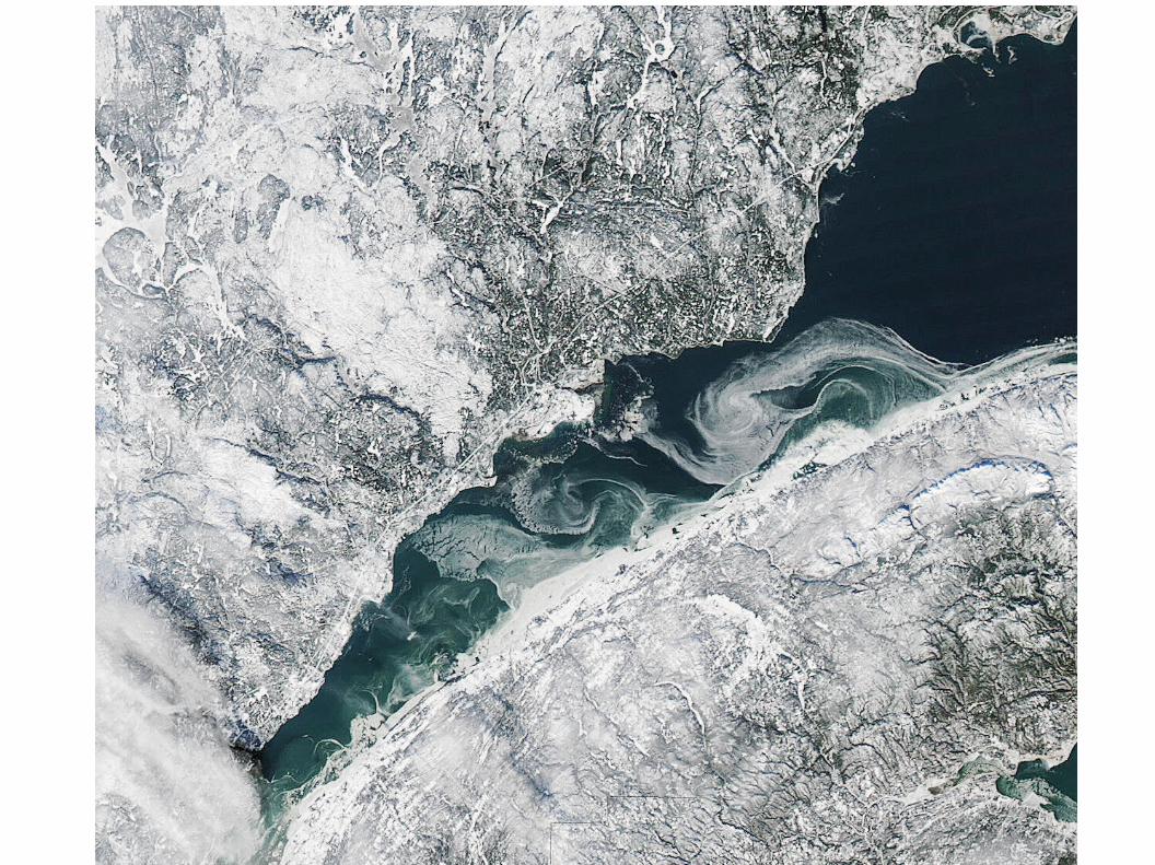
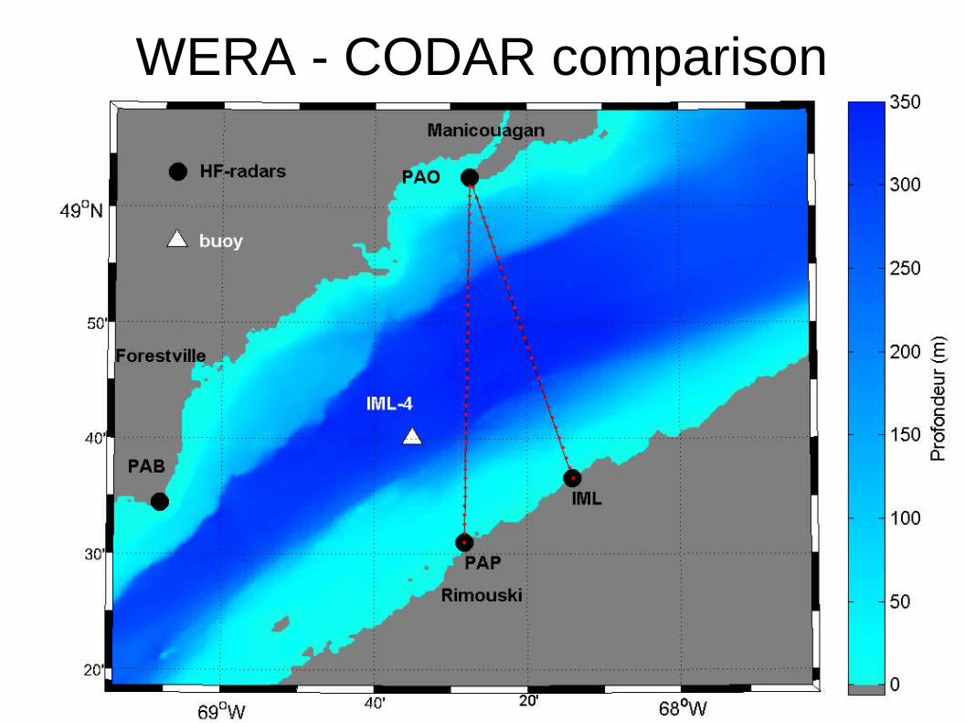
Experimental setup
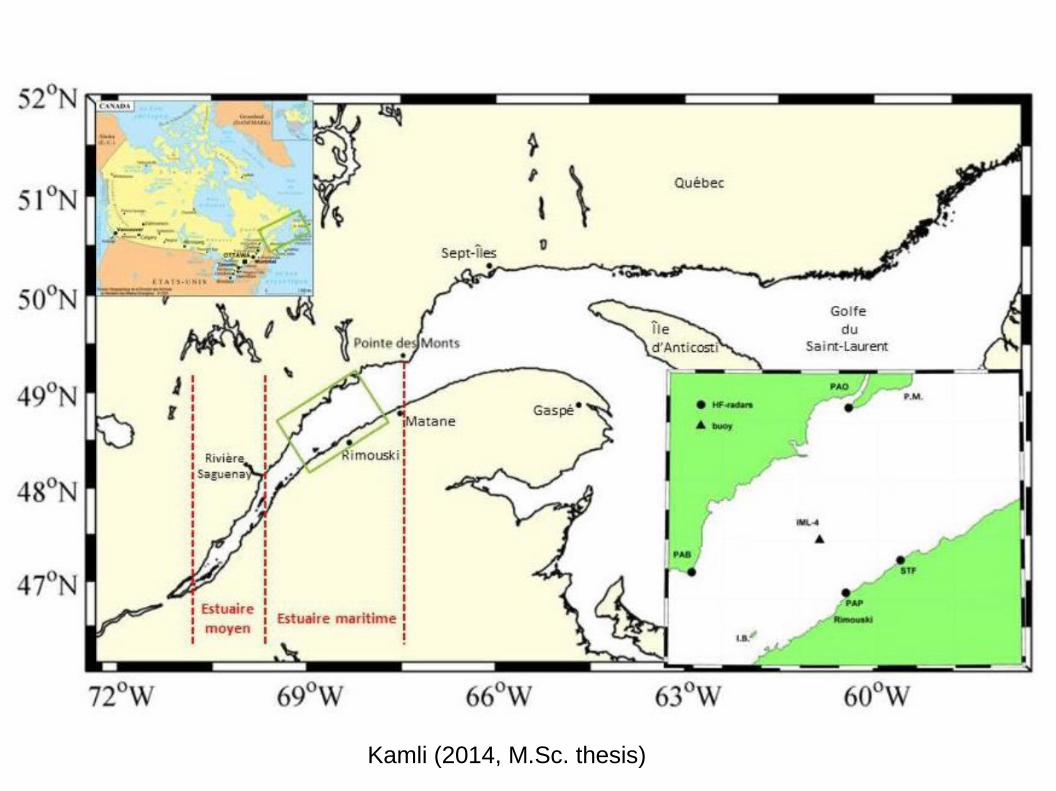
Kamli (2014, M.Sc. thesis)
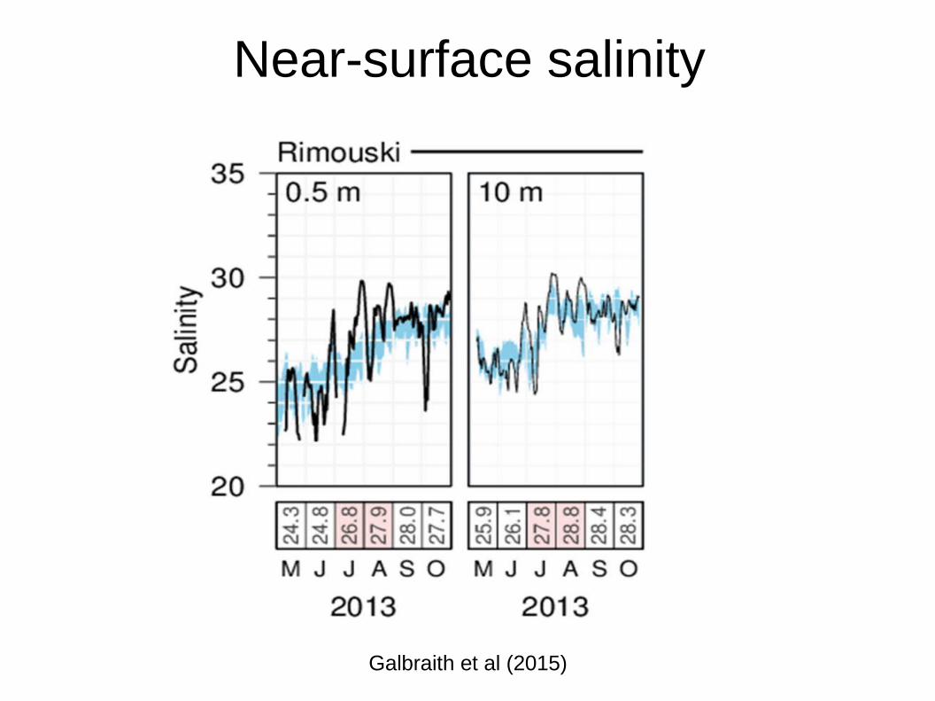
Near-surface salinity
Galbraith et al (2015)
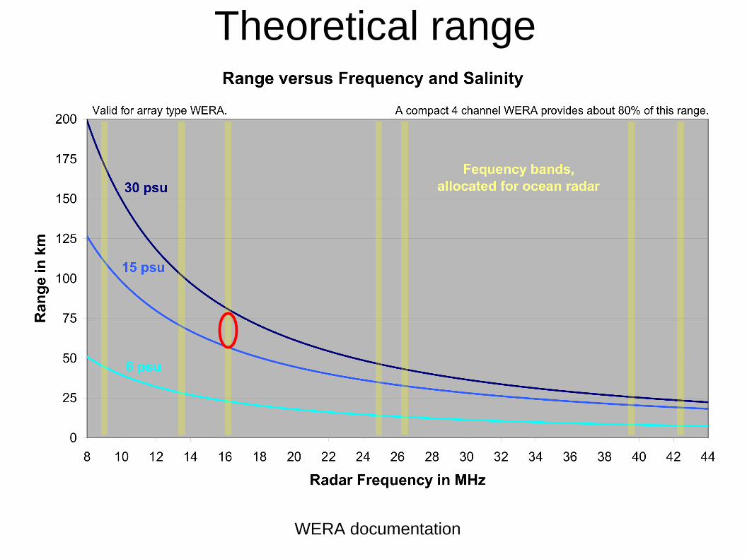
Theoretical range
WERA documentation
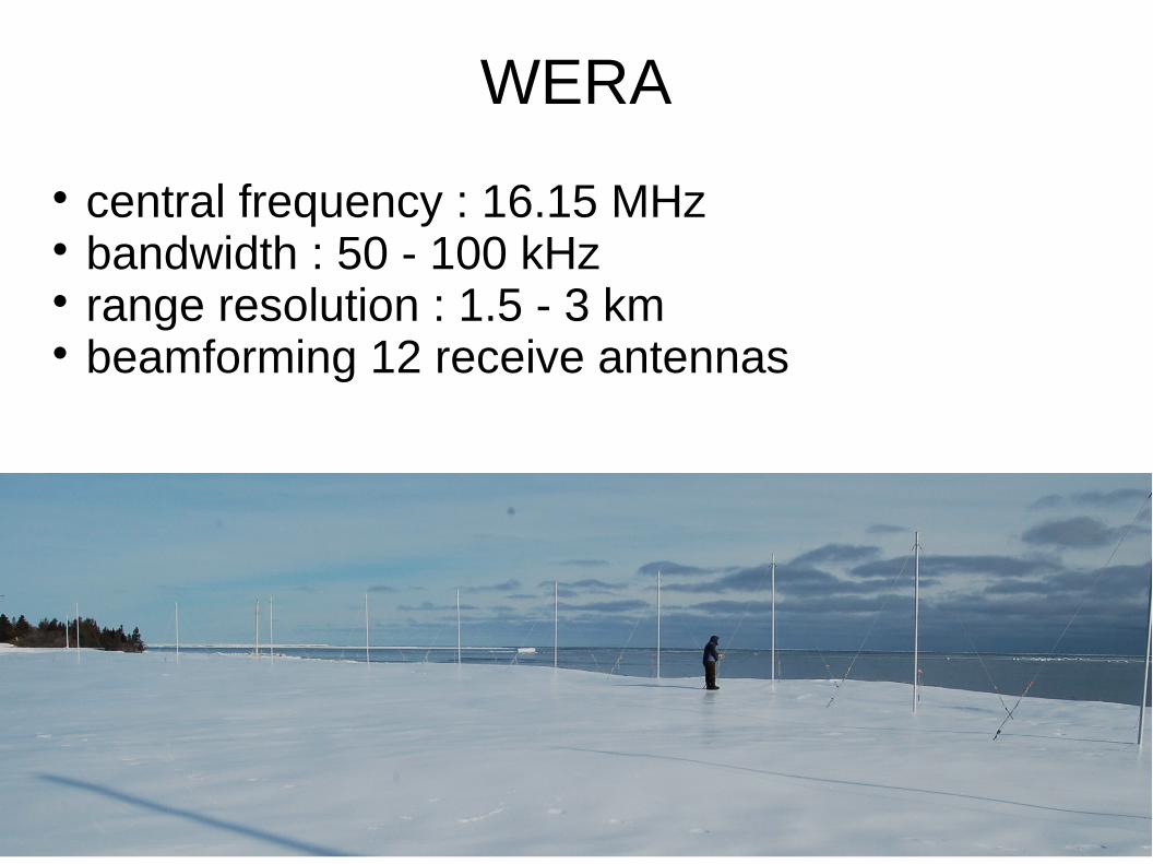
WERA
central frequency : 16.15 MHz bandwidth : 50 - 100 kHz range resolution : 1.5 - 3 km beamforming 12 receive antennas
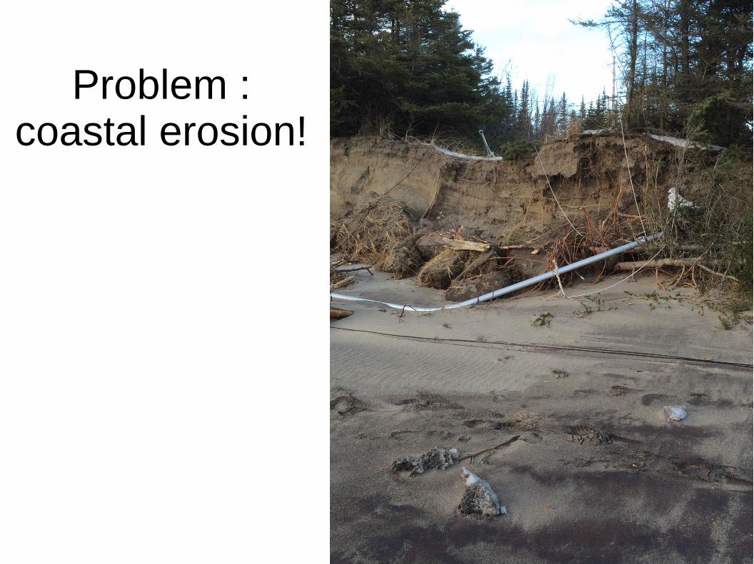
Problem : coastal erosion!
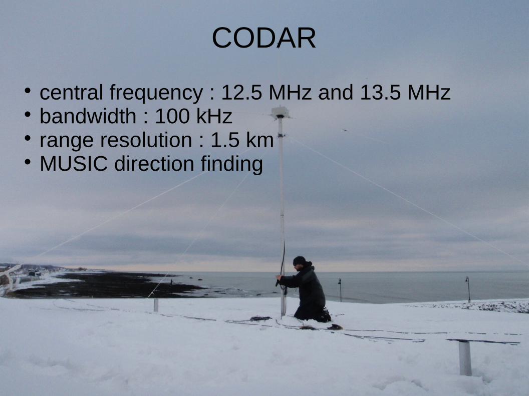
CODAR
central frequency : 12.5 MHz and 13.5 MHz bandwidth : 100 kHz range resolution : 1.5 km MUSIC direction finding
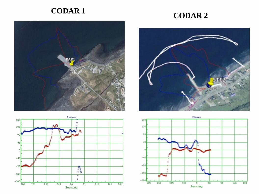
CODAR 2CODAR 1
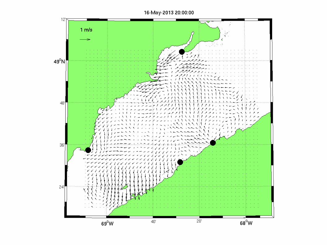
Example of currents coverage
Range vs environmental parameters
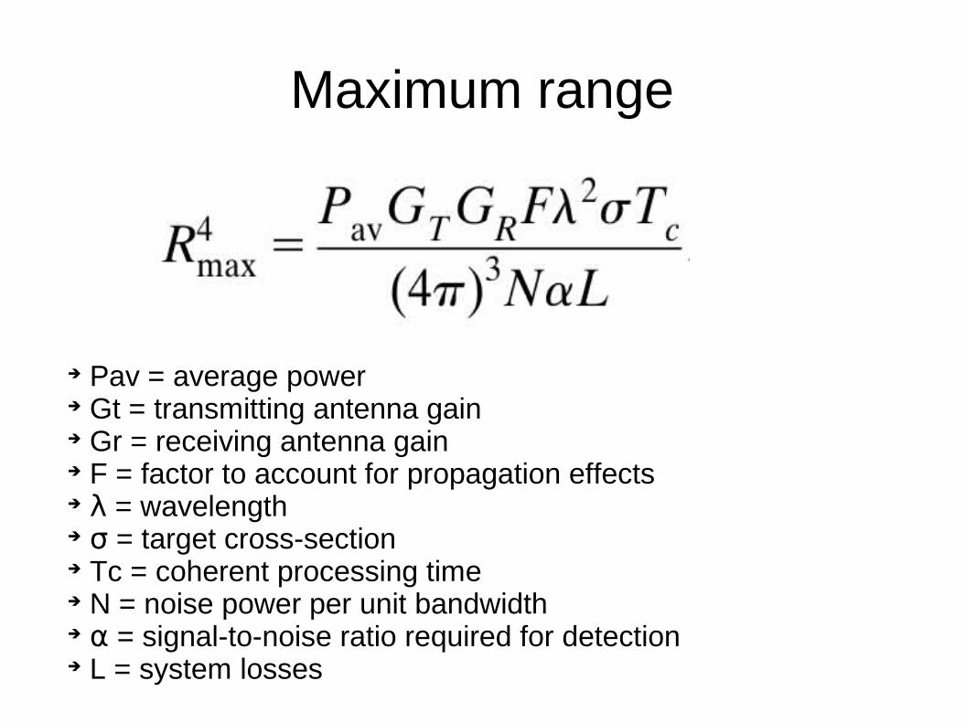
Maximum range
➔ Pav = average power➔ Gt = transmitting antenna gain➔ Gr = receiving antenna gain➔ F = factor to account for propagation effects➔ λ = wavelength➔ σ = target cross-section➔ Tc = coherent processing time➔ N = noise power per unit bandwidth➔ α = signal-to-noise ratio required for detection➔ L = system losses
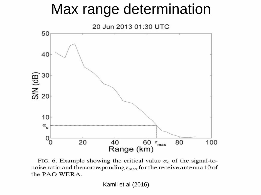
Max range determination
Kamli et al (2016)
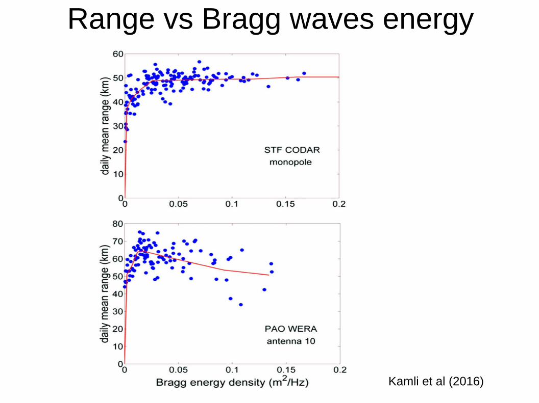
Range vs Bragg waves energy
Kamli et al (2016)
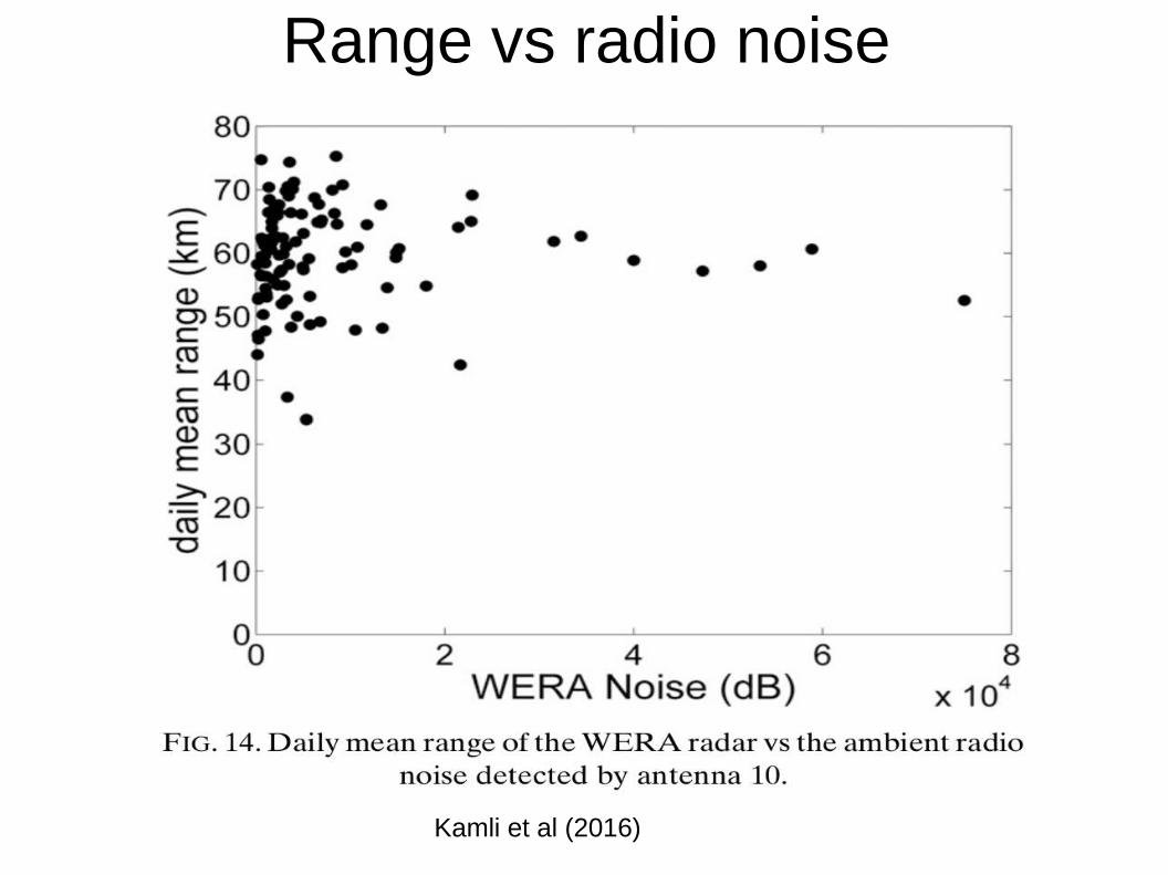
Range vs radio noise
Kamli et al (2016)
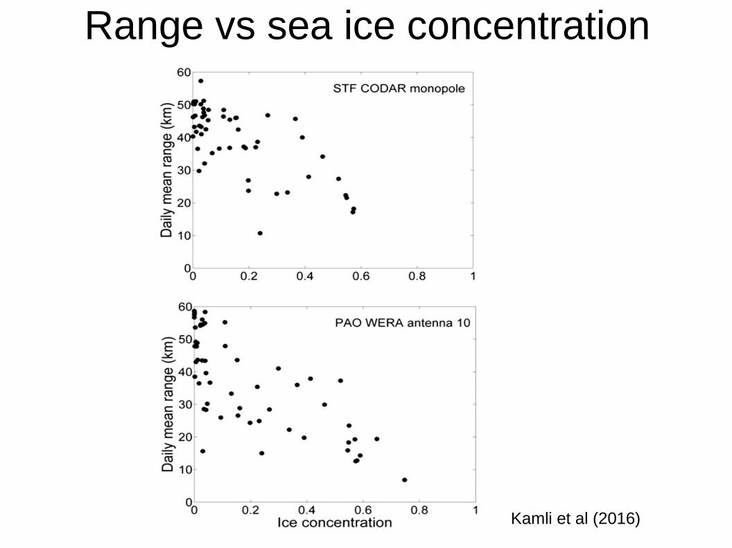
Range vs sea ice concentration
Kamli et al (2016)
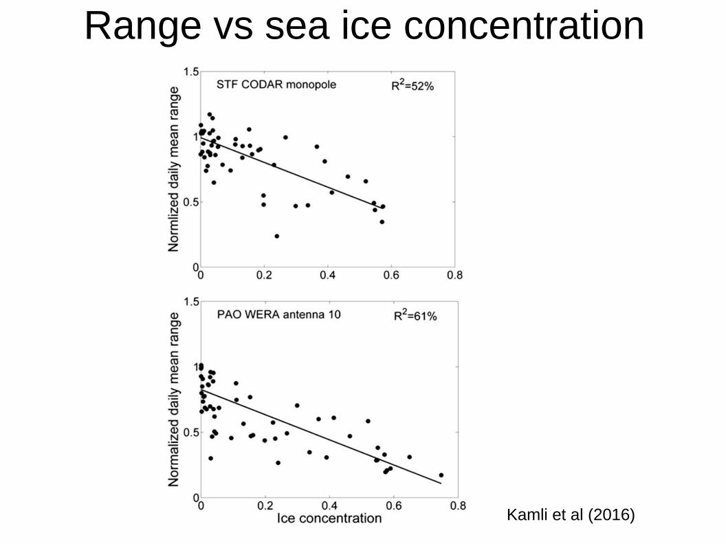
Range vs sea ice concentration
Kamli et al (2016)
Currents comparisons between WERA, CODAR, ADCP
and surface drifters
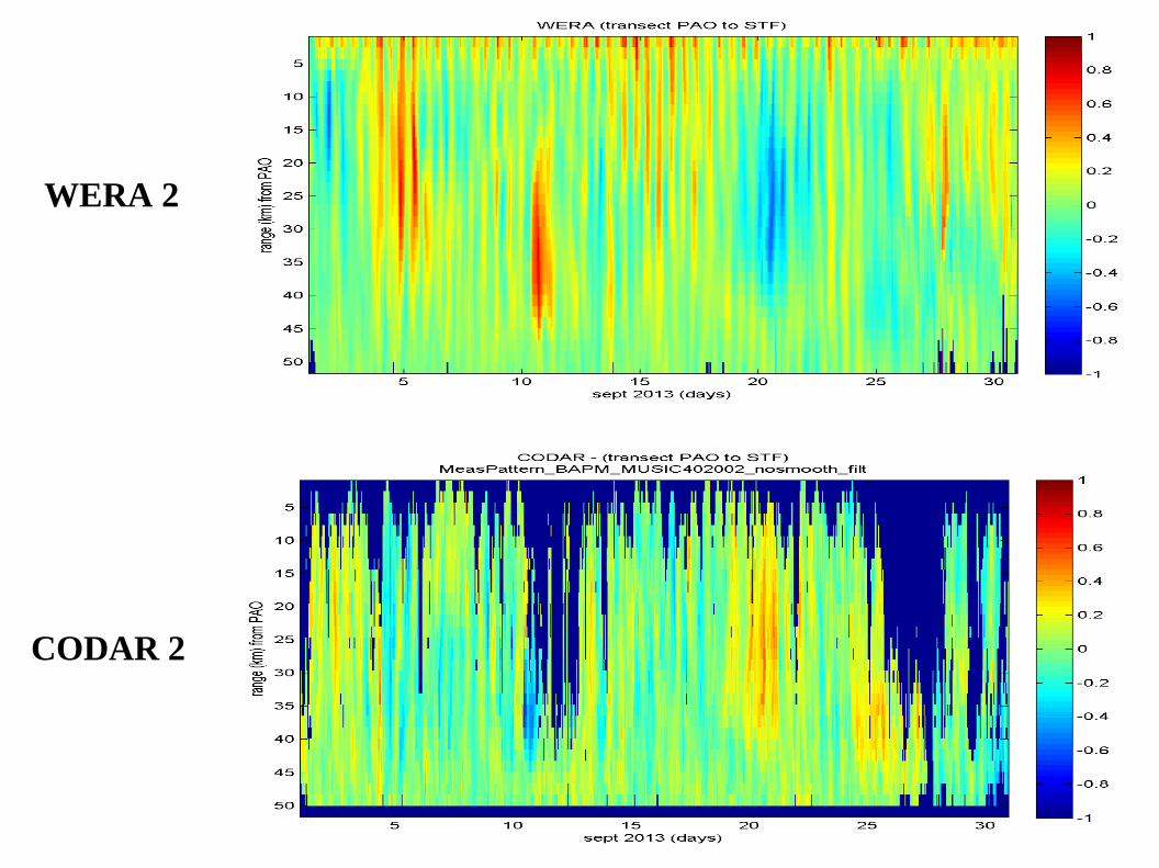
WERA - CODAR comparison
WERA 2
CODAR 2
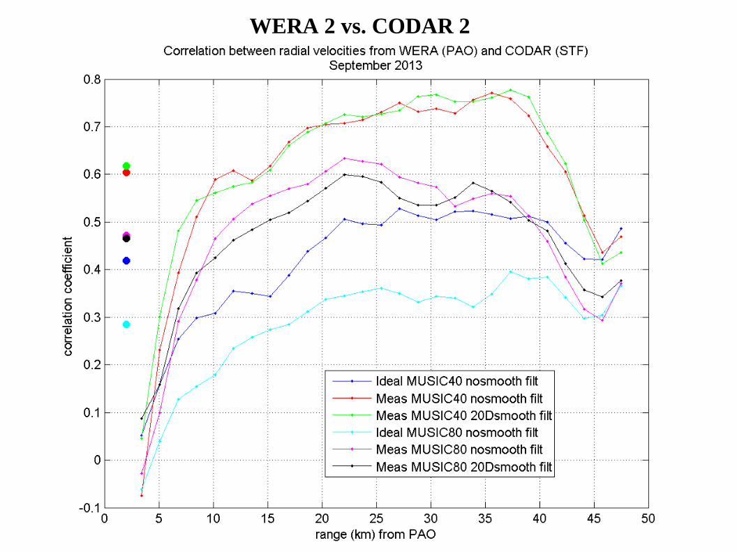
WERA 2 vs. CODAR 2
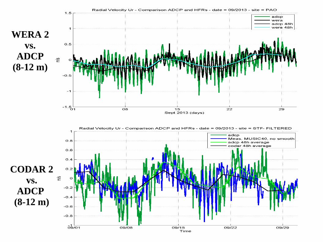
WERA 2vs.
ADCP(8-12 m)
CODAR 2vs.
ADCP (8-12 m)
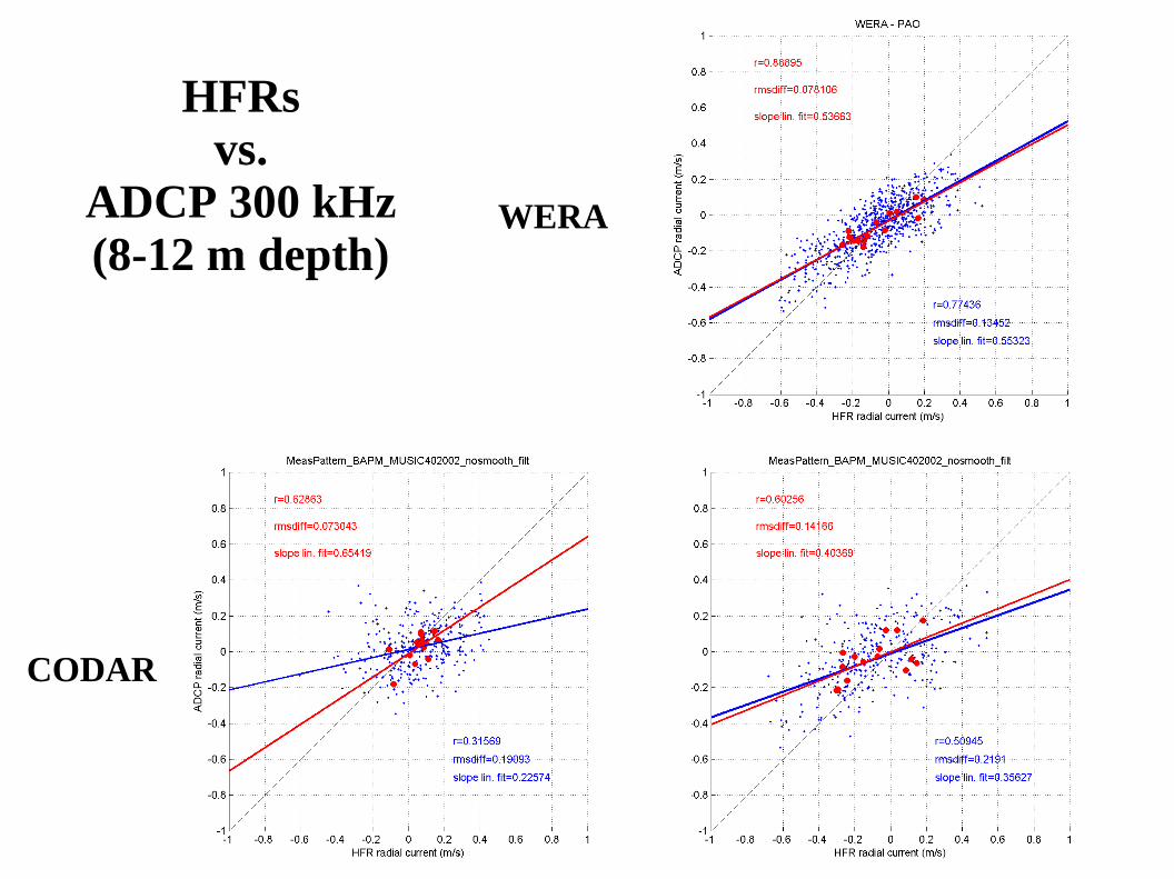
HFRsvs.
ADCP 300 kHz(8-12 m depth)
WERA
CODAR
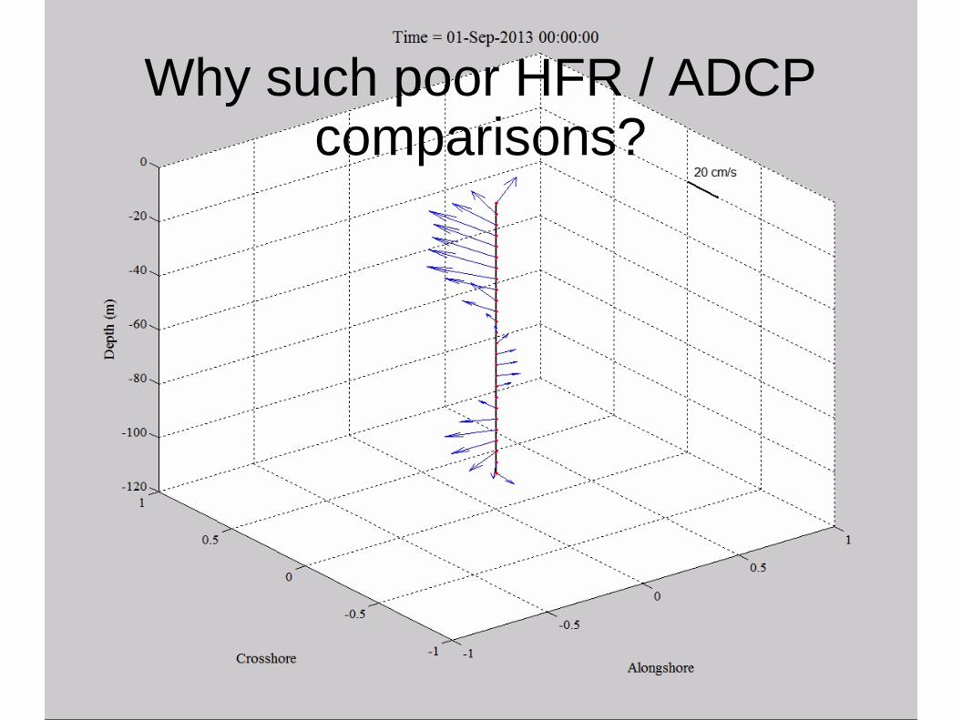
Why such poor HFR / ADCP comparisons?
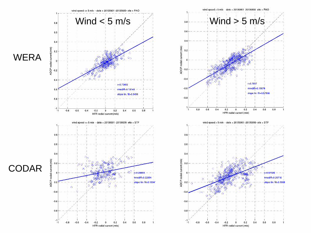
WERA
CODAR
Wind < 5 m/s Wind > 5 m/s
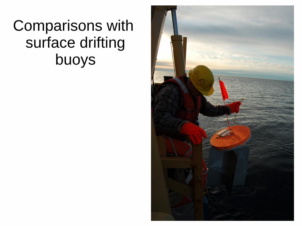
Comparisons with surface drifting
buoys
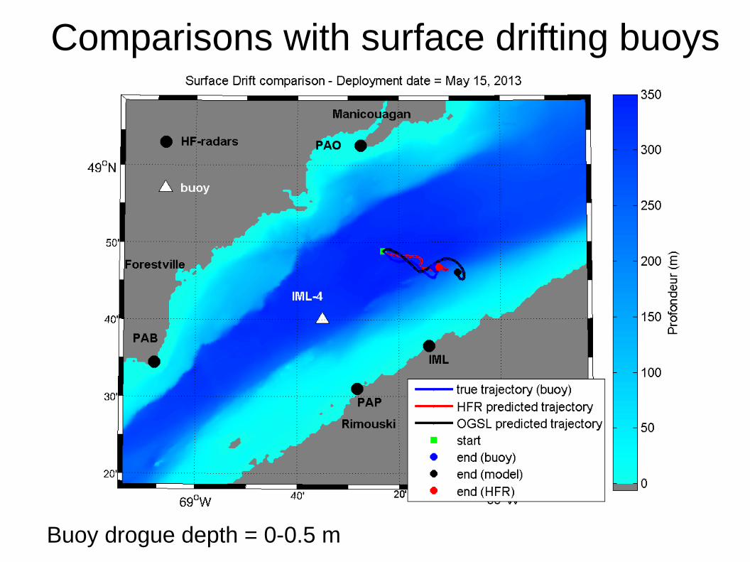
Comparisons with surface drifting buoys
Buoy drogue depth = 0-0.5 m
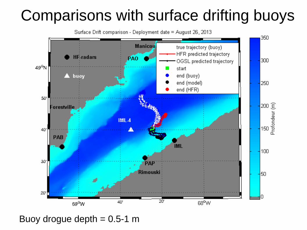
Comparisons with surface drifting buoys
Buoy drogue depth = 0.5-1 m
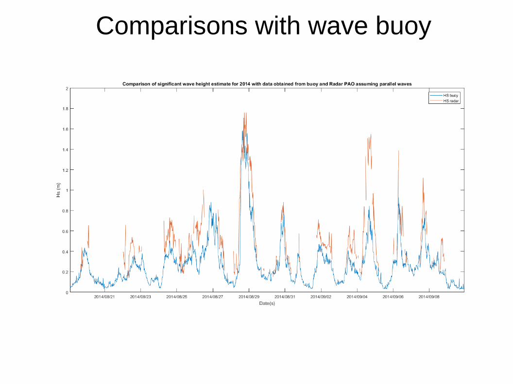
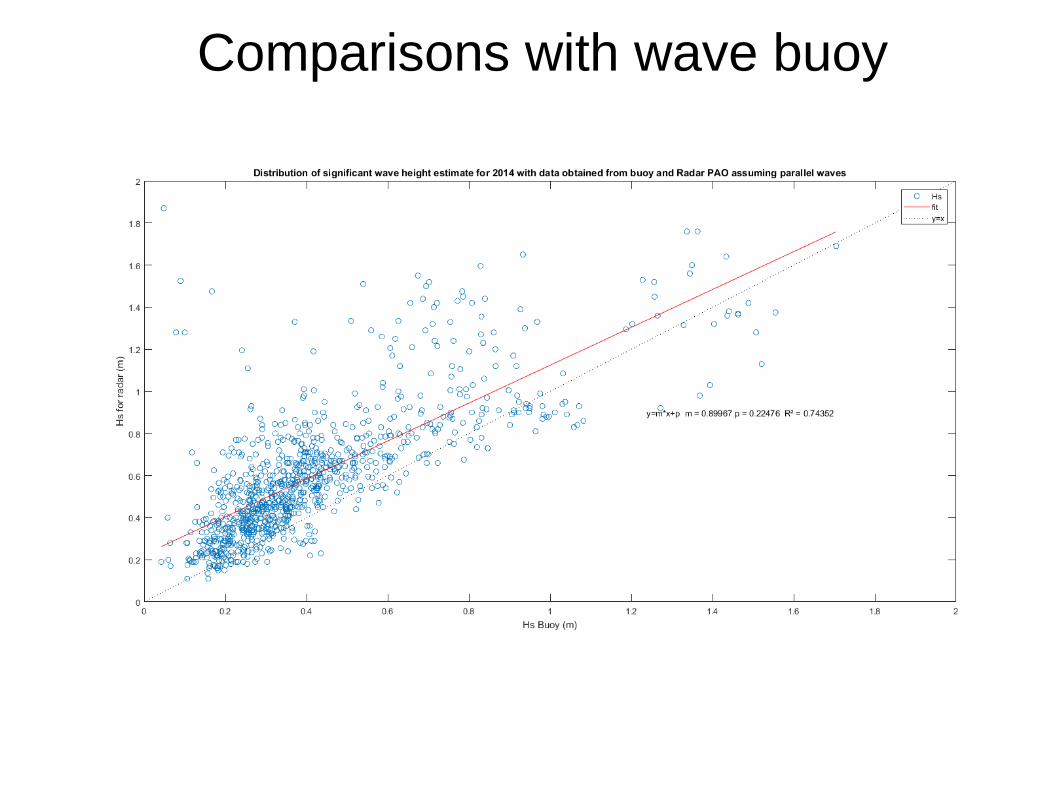
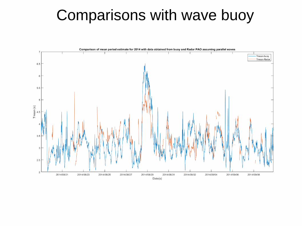
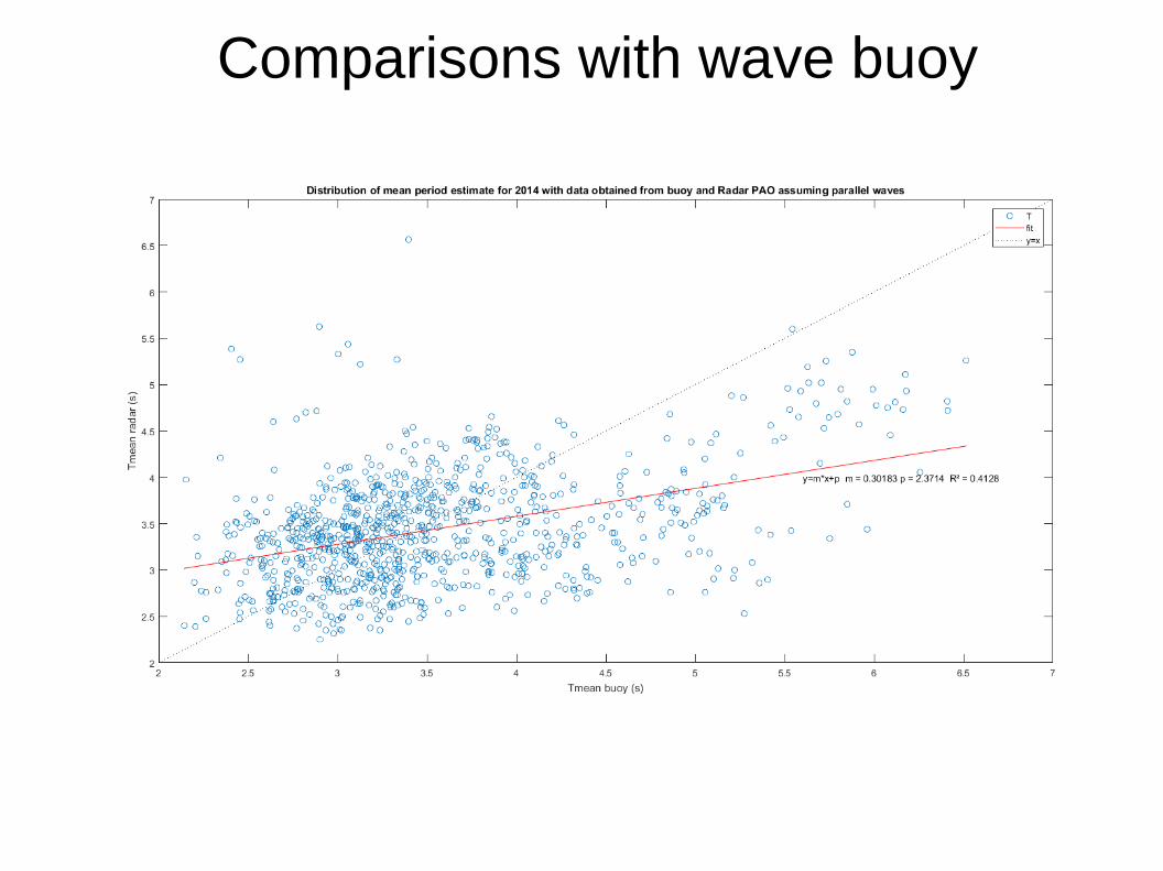
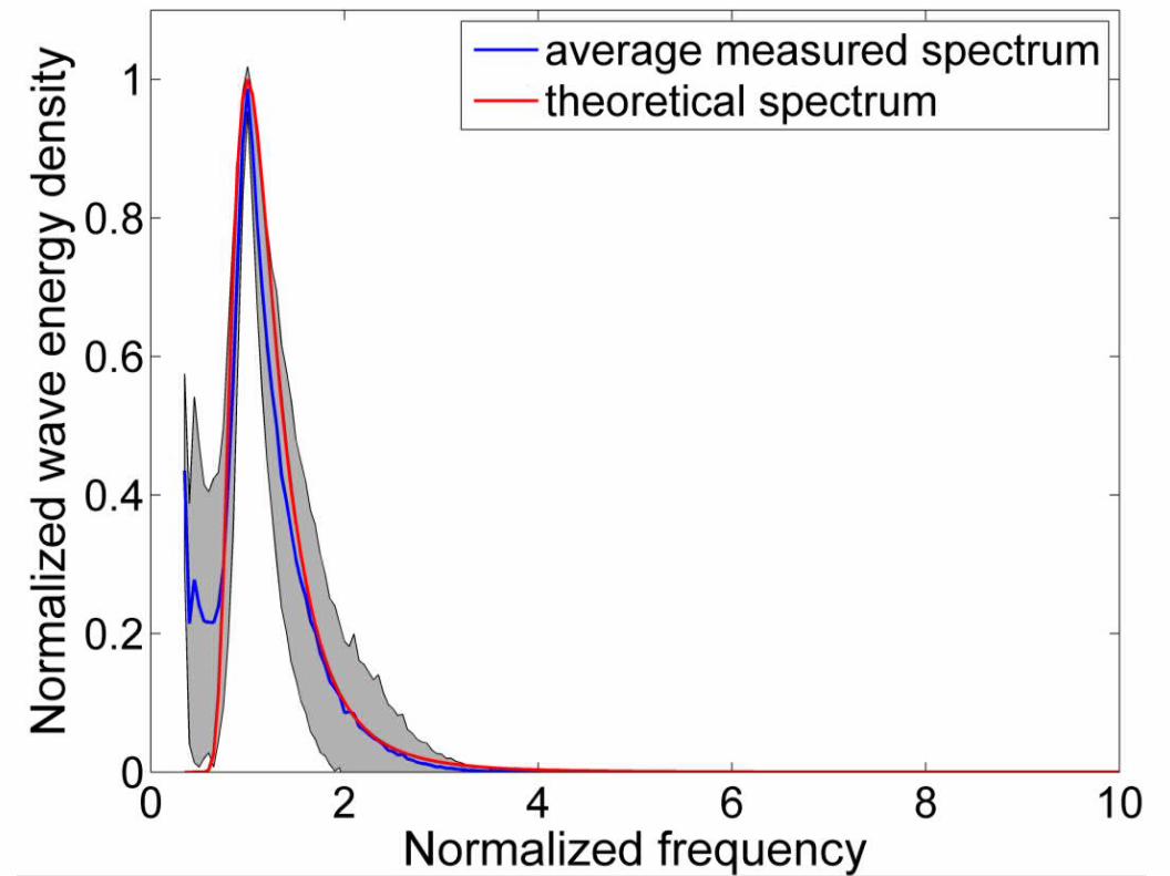
Waves comparisons between WERA and wave buoy
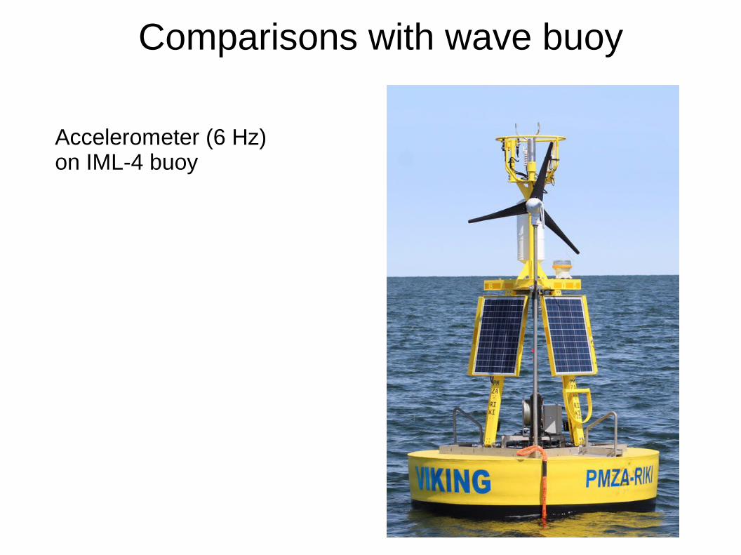
Comparisons with wave buoy
Accelerometer (6 Hz)on IML-4 buoy
Comparisons with wave buoy
Comparisons with wave buoy
Comparisons with wave buoy
Comparisons with wave buoy
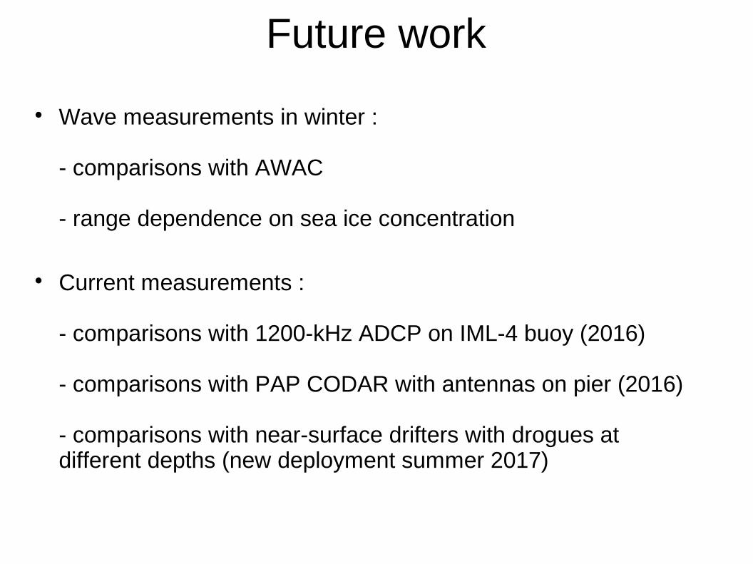
Future work
Wave measurements in winter :
- comparisons with AWAC
- range dependence on sea ice concentration
Current measurements :
- comparisons with 1200-kHz ADCP on IML-4 buoy (2016)
- comparisons with PAP CODAR with antennas on pier (2016)
- comparisons with near-surface drifters with drogues at different depths (new deployment summer 2017)
Acknowledgments
Jan Buermans, Bruno Cayouette, Fraser Eaton, Noah Hansen, Emna Kamli, Matthias Kniephoff, Julien Robitaille, Mike Scott, Markus Valentin, and Chad Whelan for installation, tuning and maintenance of HF-radars.
Ministère des Transports du Québec, Parc Nature de Pointe-aux-Outardes, Site Historique Maritime de Pointe-au-Père, and Motel Le Gaspésiana for hosting the radars on their land properties.
Ministère des Pêches et des Océans (Maurice-Lamontagne Institute) for moored ADCP data.
Développement Économique Canada pour les régions du Québec (DEC), Fonds de Recherche du Québec - Nature et Technologies (FRQNT), Natural Sciences and Engineering Research Council of Canada (NSERC), and Marine Environmental Observation Prediction and Response Network (MEOPAR) for funding.