HÖGSKOLAN DALARNA SCHOOL OF TECHNOLOGY AND BUSINESS STUDIES

MODELLING AND FORECASTING INFLATION RATES IN GHANA:

AN APPLICATION OF SARIMA MODELS

Author:

AIDOO, ERIC

Supervisor

DAO LI

APRIL, 2010

i

HÖGSKOLAN DALARNA SCHOOL OF TECHNOLOGY AND BUSINESS STUDIES

MODELLING AND FORECASTING INFLATION RATES IN GHANA:

AN APPLICATION OF SARIMA MODELS

Author

AIDOO, ERIC1

Supervisor

Dao Li

(Master‟s Thesis)

A dissertation submitted to the School of Technology and Business Studies,

Hogskolan Dalarna in partial fulfillment of the requirement for the award of

Master of Science Degree in Applied Statistics.

APRIL, 2010

1 Contact: ghanaogonos@yahoo.com or eaogonos@gmail.com or h09eriai@du.se

ii

ACKNOWLEDGEMENT

(Showing gratitude paves way for future assistance)

The completion of this research has been possible through the help of many individuals

who supported me in the different stages of this study. I would like to express my deepest

appreciation to my supervisor Dao Li. Who despite her heavy schedule has rendered me

immeasurable supports by reviewed the manuscript. Her comments and suggestions

immensely enriched the content of this work.

I am also grateful to all the lecturers and entire staffs of Dalarna University especially

Professor Kenneth Carling, Professor Changli He, Associate Professor Lars Rönnegard,

Moudud Alam, Richard Stridbeck and Mikael Moller.

I have also benefited from the help of the many other individuals during my studies at

Dalarna University, especially Collins Armah, Amarfio Susana, Fransisca Mensah, Seth

Opoku and Emmanuel Atta Boadi.

I extend my sincere gratitude to officials of Ghana Statistical Service Department for their

assistance in providing data for this exercise.

Finally, I want to give thanks to the 2010 year group of Masters in Applied Statistics,

Hogskolan Dalarna.

iii

DEDICATION

To my beloved siblings (David, Olive, Beatrice and Maxwell) and all my friends

iv

ABSTRACT

Ghana faces a macroeconomic problem of inflation for a long period of time. The problem

in somehow slows the economic growth in this country. As we all know, inflation is one of

the major economic challenges facing most countries in the world especially those in

African including Ghana. Therefore, forecasting inflation rates in Ghana becomes very

important for its government to design economic strategies or effective monetary policies

to combat any unexpected high inflation in this country. This paper studies seasonal

autoregressive integrated moving average model to forecast inflation rates in Ghana. Using

monthly inflation data from July 1991 to December 2009, we find that ARIMA

(1,1,1)(0,0,1)12 can represent the data behavior of inflation rate in Ghana well. Based on

the selected model, we forecast seven (7) months inflation rates of Ghana outside the

sample period (i.e. from January 2010 to July 2010). The observed inflation rate from

January to April which was published by Ghana Statistical Service Department fall within

the 95% confidence interval obtained from the designed model. The forecasted results

show a decreasing pattern and a turning point of Ghana inflation in the month of July.

KEY WORDS: Ghana Inflation, Forecasting, Box-Jenkins Approach, SARIMA model,

Unit Root test, ARCH–LM test, ADF test, HEGY test, Ljung-Box test.

v

TABLE OF CONTENTS

ACKNOWLEDGEMENT ................................................................................................ ii

DEDICATION .................................................................................................................. iii

ABSTRACT ...................................................................................................................... iv

TABLE OF CONTENTS .................................................................................................. v

LIST OF TABLES ........................................................................................................... vi

LIST OF FIGURES ........................................................................................................ vii

1 INTRODUCTION .......................................................................................................... 1

2 DATA .............................................................................................................................. 4

3 METHODOLOGY ......................................................................................................... 6

4 MODELLING .............................................................................................................. 13

4.1 Model Identification ................................................................................................ 13

4.2 Estimation and Evaluation ...................................................................................... 15

4.3 Forecasting .............................................................................................................. 18

5 CONCLUSIONS .......................................................................................................... 20

REFERNCES .................................................................................................................. 21

vi

LIST OF TABLES

Table 3.1: Behaviour of ACF and PACF for Non-seasonal ARIMA(p,q) ......................... 9

Table 3.2: Behaviour of ACF and PACF for Pure Seasonal ARIMA(P,Q)s ..................... 9

Table 4.1: HEGY Test for Seasonal Unit Root ................................................................ 13

Table 4.2: Canova-Hansen Test for Seasonal Unit Root .................................................. 14

Table 4.3: Unit Root Test for Inflation Series in its level form ...................................... 14

Table 4.4: Unit Root Test for First Differenced Inflation Series ..................................... 14

Table 4.5: AIC and BIC for the Suggested SARIMA Models ......................................... 16

Table 4.6: Estimation of Parameters for ARIMA(1,1,1)(0,0,1)12 .................................... 17

Table 4.7: Estimation of Parameters for ARIMA(1,1,2)(0,0,1)12 .................................... 17

Table 4.8: ARCH-LM Test for Homoscedasticity ........................................................... 17

Table 4.9: Forecast Accuracy Test on Suggested SARIMA Models ............................... 18

Table 4.10: ARIMA(1,1,1)(0,0,1)12 Forecasting Results for Monthly Inflation Rate...... 19

vii

LIST OF FIGURES

Figure 2.1: Monthly Inflation Rates of Ghana (1991:7 - 2009:12) .................................... 4

Figure 2.2: ACF and PACF of Inflation Rates (1991:7 - 2009:12).................................... 4

Figure 4.1: ACF and PACF of First Order Differenced Series ........................................ 16

Figure 4.2: Diagnostics Plot of the Residuals of ARIMA(1,1,1)(0,0,1)12 Model ............ 17

Figure 4.3: Fitted and Forecast values of ARIMA(1,1,1)(0,0,1)12 Model ....................... 19

1

1 INTRODUCTION

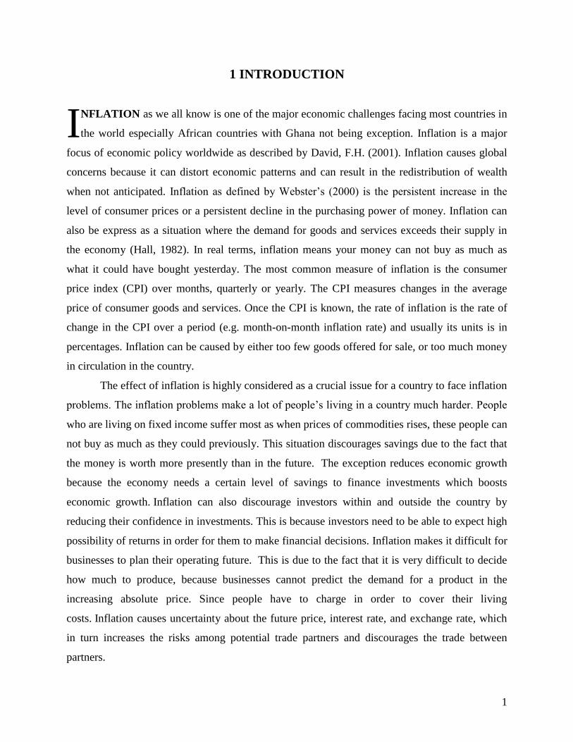
NFLATION as we all know is one of the major economic challenges facing most countries in

the world especially African countries with Ghana not being exception. Inflation is a major

focus of economic policy worldwide as described by David, F.H. (2001). Inflation causes global

concerns because it can distort economic patterns and can result in the redistribution of wealth

when not anticipated. Inflation as defined by Webster‟s (2000) is the persistent increase in the

level of consumer prices or a persistent decline in the purchasing power of money. Inflation can

also be express as a situation where the demand for goods and services exceeds their supply in

the economy (Hall, 1982). In real terms, inflation means your money can not buy as much as

what it could have bought yesterday. The most common measure of inflation is the consumer

price index (CPI) over months, quarterly or yearly. The CPI measures changes in the average

price of consumer goods and services. Once the CPI is known, the rate of inflation is the rate of

change in the CPI over a period (e.g. month-on-month inflation rate) and usually its units is in

percentages. Inflation can be caused by either too few goods offered for sale, or too much money

in circulation in the country.

The effect of inflation is highly considered as a crucial issue for a country to face inflation

problems. The inflation problems make a lot of people‟s living in a country much harder. People

who are living on fixed income suffer most as when prices of commodities rises, these people can

not buy as much as they could previously. This situation discourages savings due to the fact that

the money is worth more presently than in the future. The exception reduces economic growth

because the economy needs a certain level of savings to finance investments which boosts

economic growth. Inflation can also discourage investors within and outside the country by

reducing their confidence in investments. This is because investors need to be able to expect high

possibility of returns in order for them to make financial decisions. Inflation makes it difficult for

businesses to plan their operating future. This is due to the fact that it is very difficult to decide

how much to produce, because businesses cannot predict the demand for a product in the

increasing absolute price. Since people have to charge in order to cover their living

costs. Inflation causes uncertainty about the future price, interest rate, and exchange rate, which

in turn increases the risks among potential trade partners and discourages the trade between

partners.

I

2

Ghana was the first Sub-Sahara African country to gain political independence from their

European colonial rulers –Britain. Ghana has worked hard to deliver on the promise of happiness

for its people. Ghana‟s motto, “Freedom and Justice,” demonstrates its many peoples‟ courage

and perseverance for freedom, education and socio-political triumph; the results of which can be

seen all over the world. All the past governments in Ghana did their best to make a success

nation. The economy of Ghana is now considered as one of successful developing countries in

Africa and the world as a whole. When discussing the issues of inflation forecasts in Ghana, we

found that there has been little research on this study. To develop an effective monetary policy,

central banks should possess the information on the economic situation of the country. Such

information would enable central banks to predict future macroeconomic developments, see Asel

Isakova (2007).

In this study, our main objective is to model and forecast seven (7) months inflation rate

of Ghana outside the sample period. The post-sample forecasting is very important for economic

policy makers to foresee ahead of time the possible future requirements to design economic

strategies and effective monetary policies to combat any expected high inflation rates in the

country of Ghana. Forecasts will also play a crucial role in business, industry, government, and

institutional planning because many important decisions depend on the anticipated future values

of inflation rate. We also believed that this research will serve as a literature for other researchers

who wish to embark studies on inflation situation in Ghana.

In order to model the inflation rate, the study starts by analyzing the long behavior of

monthly inflation rates of Ghana from July, 1991 to December, 2009 for comprehensive

understanding. Following the Box-Jenkins approach, we apply SARIMA models to our time

series data in other to model and forecast future monthly inflation rates of Ghana. When it comes

to forecasting, there are extensive number of methods and approaches available and their relative

success or failure to outperform each other is in general conditional to the problem at hand. The

motive for choosing this type of model is based on the behaviour of our time series data. Also in

the history of inflation forecasting, this model has proved to perform better as compared to other

models.

Box and Jenkins (1976) propose an entire family of models, called AutoRegressive

Integrated Moving Average (ARIMA) models. It seems applicable to a wide variety of situations.

They have also developed a practical procedure for choosing an appropriate ARIMA model out

3

of this family of ARIMA models. However, selecting an appropriate ARIMA model may not be

easy. Many literatures suggest that building a proper ARIMA model is an art that requires good

judgment and a lot of experience. ARIMA models are especially suited for short term forecasting.

This is because the model places more emphasis on the recent past rather than distant past. This

emphasis on the recent past means that long-term forecasts from ARIMA models are less reliable

than short-term forecasts, see Pankratz (1983). Seasonal AutoRegressive Integrated Moving

Average (SARIMA) model is an extension of the ordinary ARIMA model to analyze time series

data which contain seasonal and non-seasonal behaviors. SARIMA model accounts for the

seasonal property in the time series. It has been found to be widely applicable in modeling

seasonal time series as well as forecasting future values. SARIMA model has also been applied to

forecast inflation extensively. The forecasting advantage of SARIMA model compared to other

time series models have been investigated by many studies. For example, Aidan et al (1998) used

SARIMA model to forecast Irish Inflation, Junttila (2001) applied SARIMA model approach in

other to forecast finish inflation, and Pufnik and Kunovac (2006) applied SARIMA model to

forecast short term inflation in Croatia. In most of those researches, SARIMA model tends to

perform better in terms of forecasting compared to other competent time series models. Schulze

and Prinz (2009) applied SARIMA model and Holt-Winters exponential smoothing approach to

forecast container transshipment in Germany, according to their results, SARIMA approach

yields slightly better values of modeling the container throughput than the exponential smoothing

approach.

The structure of the remaining paper is as follows: Section 2 describes the Inflation rate

data and macroeconomic background in Ghana. Section 3 introduces the studied SARIMA model

in this research. Section 4 analyzes our inflation data and illustrates how the theoretical

methodology can be applied for modeling and forecasting. Section 5 presents the concluding

remarks which include findings, comments and recommendations.

4

2 DATA

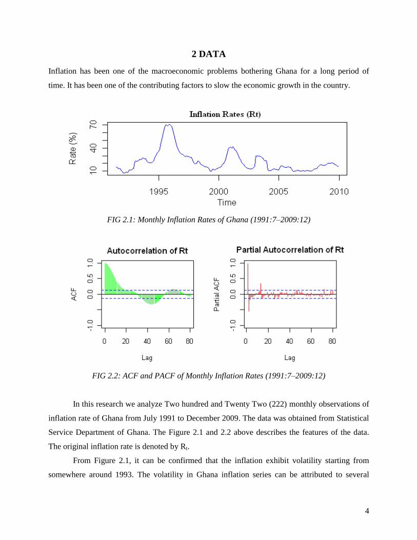
Inflation has been one of the macroeconomic problems bothering Ghana for a long period of

time. It has been one of the contributing factors to slow the economic growth in the country.

FIG 2.1: Monthly Inflation Rates of Ghana (1991:7–2009:12)

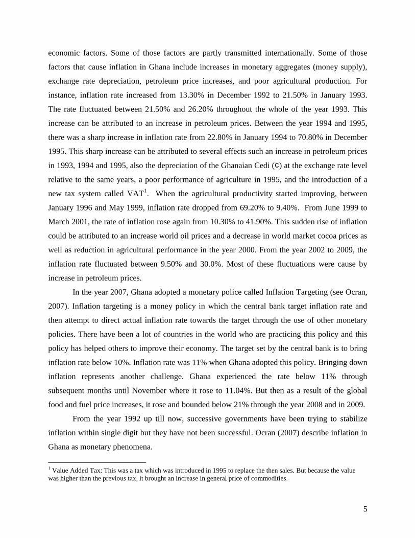
FIG 2.2: ACF and PACF of Monthly Inflation Rates (1991:7–2009:12)

In this research we analyze Two hundred and Twenty Two (222) monthly observations of

inflation rate of Ghana from July 1991 to December 2009. The data was obtained from Statistical

Service Department of Ghana. The Figure 2.1 and 2.2 above describes the features of the data.

The original inflation rate is denoted by Rt.

From Figure 2.1, it can be confirmed that the inflation exhibit volatility starting from

somewhere around 1993. The volatility in Ghana inflation series can be attributed to several

5

economic factors. Some of those factors are partly transmitted internationally. Some of those

factors that cause inflation in Ghana include increases in monetary aggregates (money supply),

exchange rate depreciation, petroleum price increases, and poor agricultural production. For

instance, inflation rate increased from 13.30% in December 1992 to 21.50% in January 1993.

The rate fluctuated between 21.50% and 26.20% throughout the whole of the year 1993. This

increase can be attributed to an increase in petroleum prices. Between the year 1994 and 1995,

there was a sharp increase in inflation rate from 22.80% in January 1994 to 70.80% in December

1995. This sharp increase can be attributed to several effects such an increase in petroleum prices

in 1993, 1994 and 1995, also the depreciation of the Ghanaian Cedi (¢) at the exchange rate level

relative to the same years, a poor performance of agriculture in 1995, and the introduction of a

new tax system called VAT1. When the agricultural productivity started improving, between

January 1996 and May 1999, inflation rate dropped from 69.20% to 9.40%. From June 1999 to

March 2001, the rate of inflation rose again from 10.30% to 41.90%. This sudden rise of inflation

could be attributed to an increase world oil prices and a decrease in world market cocoa prices as

well as reduction in agricultural performance in the year 2000. From the year 2002 to 2009, the

inflation rate fluctuated between 9.50% and 30.0%. Most of these fluctuations were cause by

increase in petroleum prices.

In the year 2007, Ghana adopted a monetary police called Inflation Targeting (see Ocran,

2007). Inflation targeting is a money policy in which the central bank target inflation rate and

then attempt to direct actual inflation rate towards the target through the use of other monetary

policies. There have been a lot of countries in the world who are practicing this policy and this

policy has helped others to improve their economy. The target set by the central bank is to bring

inflation rate below 10%. Inflation rate was 11% when Ghana adopted this policy. Bringing down

inflation represents another challenge. Ghana experienced the rate below 11% through

subsequent months until November where it rose to 11.04%. But then as a result of the global

food and fuel price increases, it rose and bounded below 21% through the year 2008 and in 2009.

From the year 1992 up till now, successive governments have been trying to stabilize

inflation within single digit but they have not been successful. Ocran (2007) describe inflation in

Ghana as monetary phenomena.

1 Value Added Tax: This was a tax which was introduced in 1995 to replace the then sales. But because the value

was higher than the previous tax, it brought an increase in general price of commodities.

6

3 METHODOLOGY

SARIMA - Seasonal AutoRegressive Integrated Moving Average model is an extension of

AutoRegressive Integrated Moving Average (ARIMA) model. The ARIMA model is a

combination of two univariate time series model which are Autoregressive (AR) model and

Moving Average (MA) model. These models are to utilize past information of a time series to

forecast future values for the series. The ARIMA model is applied in the case where the series is

non-stationary and an initial differencing step (corresponding to the "integrated" part of the

model) can make ARMA model applicable to a integrated stationary process. The ARIMA model

with its order is presented as ARIMA (p,d,q) model where p, d, and q are integers greater than or

equal to zero and refer to the order of the autoregressive, integrated, and moving average parts of

the model respectively. The first parameter p refers to the number of autoregressive lags (not

counting the unit roots), the second parameter d refers to the order of integration that makes the

data stationary, and the third parameter q gives the number of moving average lags. (see Hurvich

and Tsai, 1989; Kirchgässner and Wolters, 2007; Kleiber and Zeileis, 2008; Pankratz, 1983;

Pfaff, 2008)

A process, }{ ty is said to be ARIMA (p,d,q) if t

d

t

d yLy )1( is ARMA(p,q). In

general, we will write the model as

),0(~}{;)()1)(( 2 WNLyLL ttt

d (1)

where t follows a white noise (WN). Here, we define the Lag operator by ktt

k yyL and the

autoregressive operator and moving average operator are defined as follows:

p

p LLLL 2

211)( (2)

q

q LLLL 2

211)( (3)

0)( L for 1 , the process }{ ty is stationary if and only if d=0, in which case

it reduces to an ARMA(p,q) process.

The extension of ARIMA model to the SARIMA model comes in when the series

contains both seasonal and non-seasonal behavior. This behavior of the series makes the ARIMA

model inefficient to be applied to the series. This is because it may not be able to capture the

behavior along the seasonal part of the series and therefore mislead to a wrong order selection for

7

non-seasonal component. The SARIMA model is sometimes called the multiplicative seasonal

autoregressive integrated moving average denoted by ARIMA(p,d,q)x(P,D,Q)S. This can be

written in is lag form as (Halim & Bisono, 2008):

t

S

t

DSdS BByBBBB )()()1()1)(()( (4)

P

P BBBB 2

211)( (5)

PS

P

SSS BBBB 2

211)( (6)

q

q BBBB 2

211)( (7)

qS

q

SSS BBBB 2

211)( (8)

where,

p, d and q are the order of non-seasonal AR, differencing and MA respectively.

P, D and Q is the order of seasonal AR, differencing and MA respectively.

yt represent time series data at period t.

t represent white noise error (random shock) at period t.

B represent backward shift operator ( ktt

k yyB )

S represent seasonal order ( 4s for quarterly data and 12s for monthly data).

In the identification stage of model building, we determine the possible models based on

the data pattern. But before we can begin to search for the best model for the data, the first

condition is to check whether the series is stationary or not. The ARIMA model is appropriate for

stationary time series data (i.e. the mean, variance, and autocorrelation are constant through

time). If a time series is stationary then the mean of any major subset of the series does not differ

significantly from the mean of any other major subset of the series. Also if a data series is

stationary then the variance of any major subset of the series will differ from the variance of any

other major subset only by chance (see Pankratz, 1983). The stationarity condition ensures that

the autoregressive parameters in the estimated model are stable within a certain range as well as

the moving average parameters in the model are invertible. If this condition is assured then, the

estimated model can be forecasted (see Hamilton, 1994). To check for stationarity, we usually

test for the existence or nonexistence of what we called unit root. Unit root test is performed to

determine whether a stochastic or a deterministic trend is present in the series. If the roots of the

characteristic equation (such as equation 2) lie outside the unit circle, then the series is considered

8

stationary. This is equivalent to say that the coefficients of the estimated model are in absolute

value is less than 1 (i.e. pifori ,,11 ). There are several statistical tests in testing for

presence of unit root in a series. For series with seasonal and non-seasonal behaviour, the test

must be conducted under the seasonal part as well as the non-seasonal part. Some example of the

unit root test for the non-seasonal time series are the Dickey-Fuller and the Augmented Dickey-

Fuller (DF, ADF) test, Kwiatkowski-Phillips-Schmidt-Shin (KPSS) test and Zivot-Andrews (ZA)

test (see Dickey & Fuller, 1979; Kwiatkowski et al, 1992; Zivot & Andrews, 1992). Also some

examples of the unit root test for seasonal time series are Hylleberg-Engle-Granger-Yoo

(HEGY)1 test, Canova-Hansen (CH) test etc (see Canova & Hansen,1995; Hylleberg et al,1990;

Beaulieu &Miron,1993).

When the series is stationary, the order of the model which is the AR, MA, SAR and

SMA terms can be determine. Where AR=p and MA=q represent the non-seasonal autoregressive

and moving average parts respectively and SAR=P and SMA=Q represent the seasonal

autoregressive and moving average parts respectively as described earlier. To determine these

orders, we use the sample autocorrelation function (ACF)2 and partial autocorrelation function

(PACF) of the stationary series. The ACF and PACF give more information about the behavior of

the time series. The ACF gives information about the internal correlation between observations in

a time series at different distances apart, usually expressed as a function of the time lag between

observations. These two plots suggest the model we should build. Checking the ACF and PACF

plots, we should both look at the seasonal and non-seasonal lags. Usually the ACF and the PACF

has spikes at lag k and cuts off after lag k at the non-seasonal level. Also the ACF and the PACF

has spikes at lag ks and cuts off after lag ks at the seasonal level. The number of significant

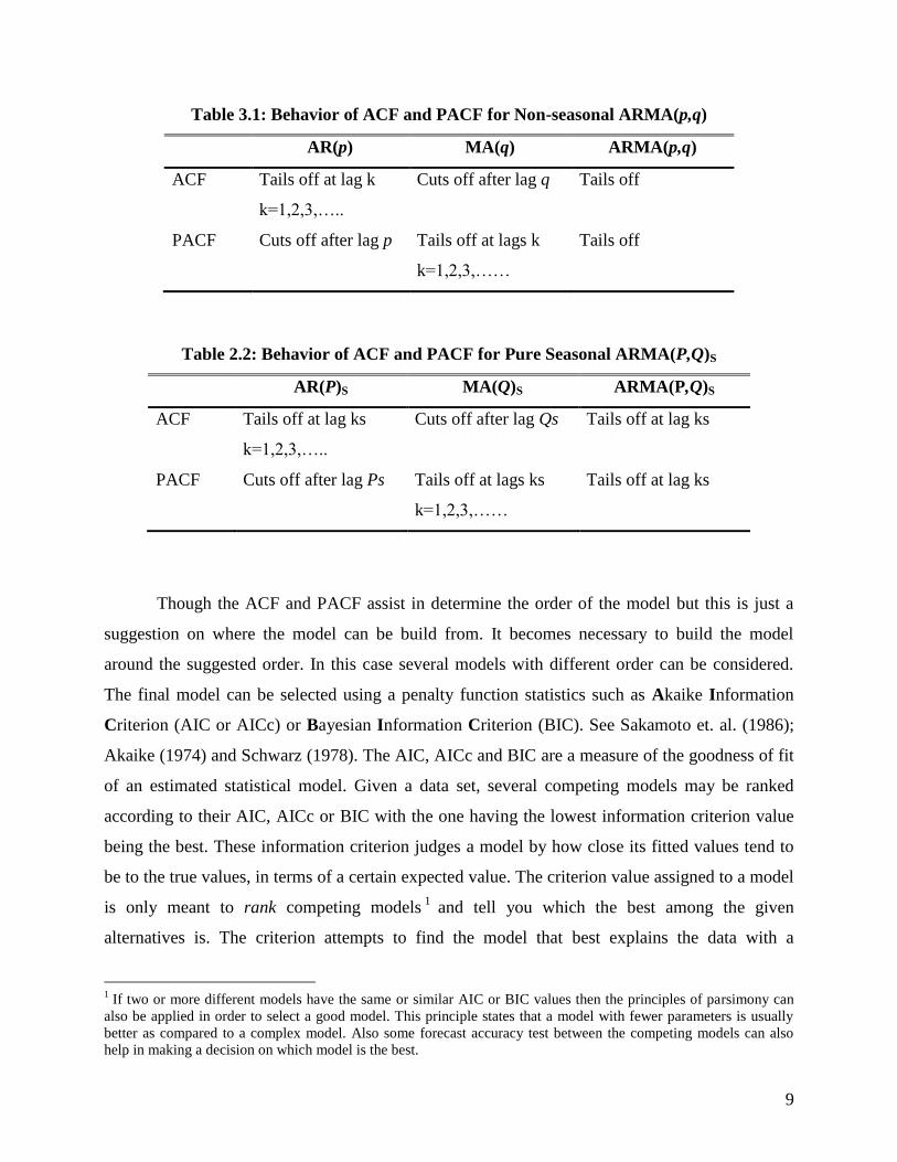
spikes suggests the order of the model. The Table 3.1 and 3.2 below describes the behaviour of

the ACF and PACF for both seasonal and the non-seasonal series (see Shumway and Stoffer,

2006)

1 The HEGY test was first applied by the authors to test for seasonal unit root in quarterly data. The test was later

extended by some to authors such as Beaulieu & Miron, to test for seasonal unit root in monthly data. The CH test

also use similar procedure but in different format. 2 The ACF and PACF are plot that display the estimated autocorrelation and partial autocorrelation coefficients after

fitting autoregressive models of successively higher orders to the time series.

9

Table 3.1: Behavior of ACF and PACF for Non-seasonal ARMA(p,q)

AR(p) MA(q) ARMA(p,q)

ACF Tails off at lag k

k=1,2,3,…..

Cuts off after lag q Tails off

PACF Cuts off after lag p Tails off at lags k

k=1,2,3,……

Tails off

Table 2.2: Behavior of ACF and PACF for Pure Seasonal ARMA(P,Q)S

AR(P)S MA(Q)S ARMA(P,Q)S

ACF Tails off at lag ks

k=1,2,3,…..

Cuts off after lag Qs Tails off at lag ks

PACF Cuts off after lag Ps Tails off at lags ks

k=1,2,3,……

Tails off at lag ks

Though the ACF and PACF assist in determine the order of the model but this is just a

suggestion on where the model can be build from. It becomes necessary to build the model

around the suggested order. In this case several models with different order can be considered.

The final model can be selected using a penalty function statistics such as Akaike Information

Criterion (AIC or AICc) or Bayesian Information Criterion (BIC). See Sakamoto et. al. (1986);

Akaike (1974) and Schwarz (1978). The AIC, AICc and BIC are a measure of the goodness of fit

of an estimated statistical model. Given a data set, several competing models may be ranked

according to their AIC, AICc or BIC with the one having the lowest information criterion value

being the best. These information criterion judges a model by how close its fitted values tend to

be to the true values, in terms of a certain expected value. The criterion value assigned to a model

is only meant to rank competing models1

and tell you which the best among the given

alternatives is. The criterion attempts to find the model that best explains the data with a

1 If two or more different models have the same or similar AIC or BIC values then the principles of parsimony can

also be applied in order to select a good model. This principle states that a model with fewer parameters is usually

better as compared to a complex model. Also some forecast accuracy test between the competing models can also

help in making a decision on which model is the best.

10

minimum of free parameters but also includes a penalty that is an increasing function of the

number of estimated parameters.

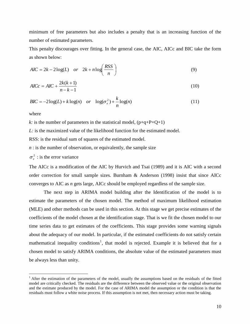
This penalty discourages over fitting. In the general case, the AIC, AICc and BIC take the form

as shown below:

n

RSSnkorLkAIC log2)log(22 (9)

1

)1(2

kn

kkAICAICc (10)

)log()log()log()log(2 2 nn

kornkLBIC e (11)

where

k: is the number of parameters in the statistical model, (p+q+P+Q+1)

L: is the maximized value of the likelihood function for the estimated model.

RSS: is the residual sum of squares of the estimated model.

n : is the number of observation, or equivalently, the sample size

2

e : is the error variance

The AICc is a modification of the AIC by Hurvich and Tsai (1989) and it is AIC with a second

order correction for small sample sizes. Burnham & Anderson (1998) insist that since AICc

converges to AIC as n gets large, AICc should be employed regardless of the sample size.

The next step in ARIMA model building after the Identification of the model is to

estimate the parameters of the chosen model. The method of maximum likelihood estimation

(MLE) and other methods can be used in this section. At this stage we get precise estimates of the

coefficients of the model chosen at the identification stage. That is we fit the chosen model to our

time series data to get estimates of the coefficients. This stage provides some warning signals

about the adequacy of our model. In particular, if the estimated coefficients do not satisfy certain

mathematical inequality conditions1, that model is rejected. Example it is believed that for a

chosen model to satisfy ARIMA conditions, the absolute value of the estimated parameters must

be always less than unity.

1 After the estimation of the parameters of the model, usually the assumptions based on the residuals of the fitted

model are critically checked. The residuals are the difference between the observed value or the original observation

and the estimate produced by the model. For the case of ARIMA model the assumption or the condition is that the

residuals must follow a white noise process. If this assumption is not met, then necessary action must be taking.

11

After estimating the parameters of ARIMA model, the next step in the Box-Jenkins

approach is to check the adequacy of that model which is usually called model diagnostics.

Ideally, a model should extract all systematic information from the data. The part of the data

unexplained by the model (i.e., the residuals) should be small. The diagnostic check is used to

determine the adequacy of the chosen model. These checks are usually based on the residuals of

the model. One assumption of the ARIMA model is that, the residuals of the model should be

white noise. A series }{ t is said to be white noise if }{ t is a sequence of independent and

identically distributed random variable with finite mean and variance. In addition if }{ t is

normally distributed with mean zero and variance 2 , then the series is called Gaussian White

Noise. For a white noise series the, all the ACF are zero. In practice if the residuals of the model

is white noise, then the ACF of the residuals are approximately zero. If the assumption of are not

fulfilled then different model for the series must be search for. A statistical tool such as Ljung-

Box Q statistic can be used to determine whether the series is independent or not. Statistical tool

such as ARCH–LM test and Shapiro normality test can also be used to check for

homoscedasticity and normality among the residuals respectively.

The last step in Box-Jenkins model building approach is Forecasting1. After a model has

passed the entire diagnostic test, it becomes adequate for forecasting. Forecasting is the process

of making statements about events whose actual outcomes have not yet been observed. It is an

important application of time series. If a suitable model for the data generation process (DGP) of

a given time series has been found, it can be used for forecasting the future development of the

variable under consideration. In ARIMA models as described by several researchers have proved

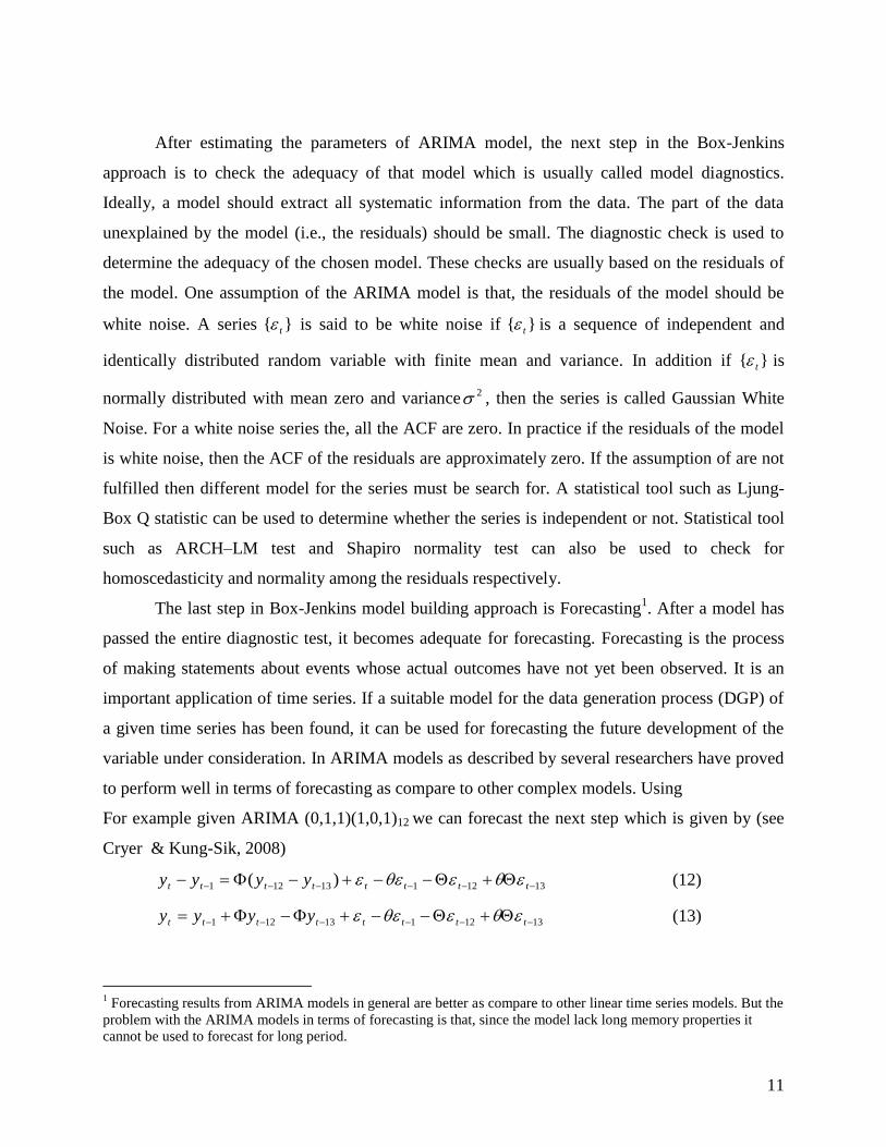
to perform well in terms of forecasting as compare to other complex models. Using

For example given ARIMA (0,1,1)(1,0,1)12 we can forecast the next step which is given by (see

Cryer & Kung-Sik, 2008)

1312113121 )( tttttttt yyyy (12)

1312113121 tttttttt yyyy (13)

1 Forecasting results from ARIMA models in general are better as compare to other linear time series models. But the

problem with the ARIMA models in terms of forecasting is that, since the model lack long memory properties it

cannot be used to forecast for long period.

12

The one step ahead forecast from the origin t is given by

121112111 ttttttt yyyy

(14)

The next step is

1110111012 tttttt yyyy

(15)

and so forth. The noise terms 110111213 ,,,,, (as residuals) will enter into the forecasts for

lead times 13,,3,2,1 l but for 13l the autoregressive part of the model takes over and we

have

1313121 lforyyyy ltltltlt

(16)

To choose a final model for forecasting the accuracy of the model must be higher than

that of all the competing models. The accuracy for each model can be checked to determine how

the model performed in terms of in-sample forecast. Usually in time series forecasting, some of

the observations are left out during model building in other to access models in terms of out of

sample forecasting also. The accuracy of the models can be compared using some statistic such

as mean error (ME), root mean square error. (RMSE), mean absolute error (MAE), mean

percentage error (MPE), mean absolute percentage error (MAPE) etc. A model with a minimum

of these statistics is considered to be the best for forecasting.

13

4 MODELLING

4.1 Model Identification

Looking at the sample ACF and PACF plot of the series in Figure 2.2, there is non-seasonal and

seasonal pattern in the series. To confirm the proper order of differencing filter, we can perform

both seasonal and non-seasonal unit root test. Using CH and HEGY test, we can test seasonal unit

root in the series. Seasonal frequencies in monthly data are 66

5,

3,

3

2,

2,

and . These are

equivalent to 6, 3, 4, 2, 5 and 1 cycles per year respectively (Hylleberg et. al,1990; Canova and

Hansen, 1995). The null hypothesis to be tested in HEGY test is, „there exist seasonal unit root‟.

Also the null hypothesis to be tested in CH test is „there exist stationarity at all seasonal cycles‟.

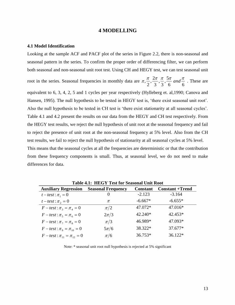
Table 4.1 and 4.2 present the results on our data from the HEGY and CH test respectively. From

the HEGY test results, we reject the null hypothesis of unit root at the seasonal frequency and fail

to reject the presence of unit root at the non-seasonal frequency at 5% level. Also from the CH

test results, we fail to reject the null hypothesis of stationarity at all seasonal cycles at 5% level.

This means that the seasonal cycles at all the frequencies are deterministic or that the contribution

from these frequency components is small. Thus, at seasonal level, we do not need to make

differences for data.

Table 4.1: HEGY Test for Seasonal Unit Root

Note: * seasonal unit root null hypothesis is rejected at 5% significant

Auxiliary Regression Seasonal Frequency Constant Constant +Trend

0: 1 testt 0 -2.123 -3.164

0: 2 testt -6.667* -6.655*

0: 43 testF 2 47.072* 47.016*

0: 65 testF 32 42.240* 42.453*

0: 87 testF 3 46.989* 47.093*

0: 109 testF 65 38.322* 37.677*

0: 1211 testF 6 36.753* 36.122*

14

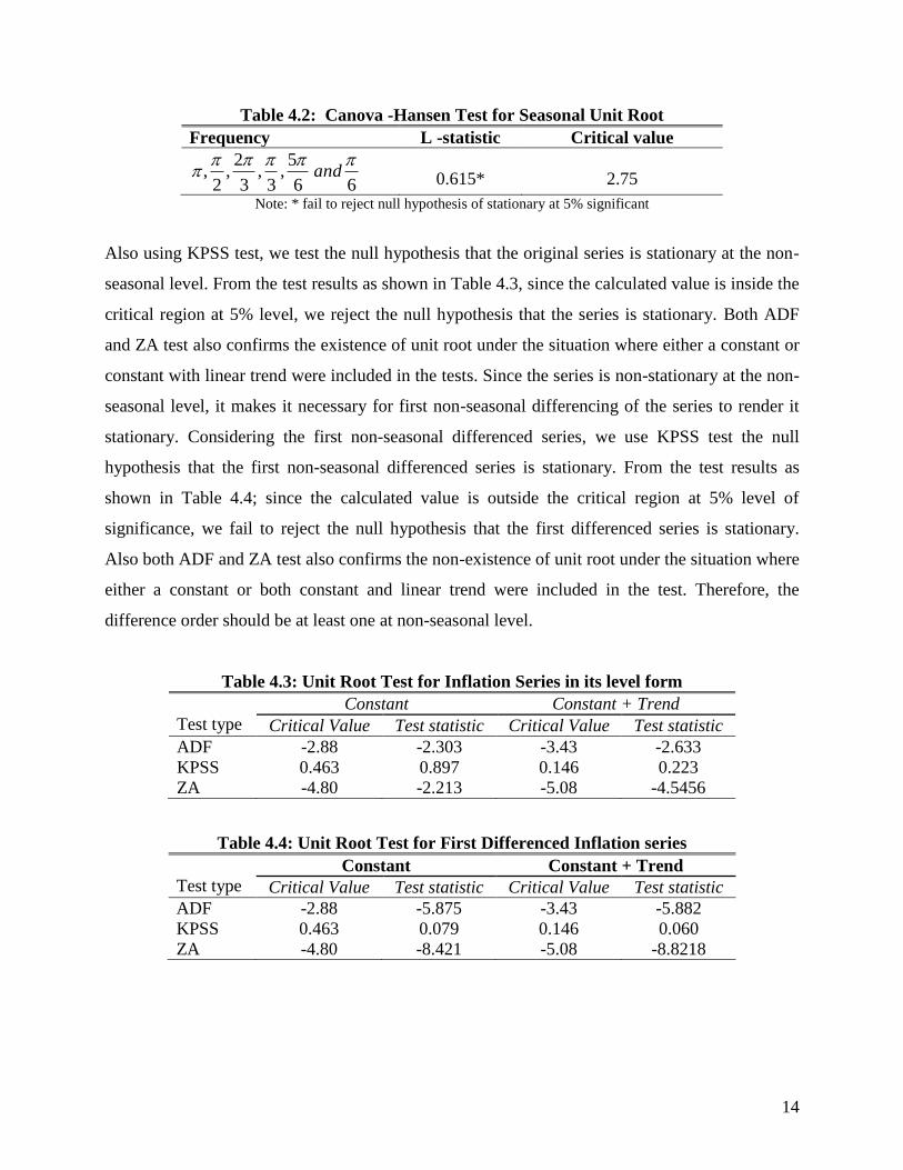
Table 4.2: Canova -Hansen Test for Seasonal Unit Root

Frequency L -statistic Critical value

66

5,

3,

3

2,

2,

and

0.615*

2.75

Note: * fail to reject null hypothesis of stationary at 5% significant

Also using KPSS test, we test the null hypothesis that the original series is stationary at the non-

seasonal level. From the test results as shown in Table 4.3, since the calculated value is inside the

critical region at 5% level, we reject the null hypothesis that the series is stationary. Both ADF

and ZA test also confirms the existence of unit root under the situation where either a constant or

constant with linear trend were included in the tests. Since the series is non-stationary at the non-

seasonal level, it makes it necessary for first non-seasonal differencing of the series to render it

stationary. Considering the first non-seasonal differenced series, we use KPSS test the null

hypothesis that the first non-seasonal differenced series is stationary. From the test results as

shown in Table 4.4; since the calculated value is outside the critical region at 5% level of

significance, we fail to reject the null hypothesis that the first differenced series is stationary.

Also both ADF and ZA test also confirms the non-existence of unit root under the situation where

either a constant or both constant and linear trend were included in the test. Therefore, the

difference order should be at least one at non-seasonal level.

Table 4.3: Unit Root Test for Inflation Series in its level form

Test type

Constant Constant + Trend

Critical Value Test statistic Critical Value Test statistic

ADF -2.88 -2.303 -3.43 -2.633

KPSS 0.463 0.897 0.146 0.223

ZA -4.80 -2.213 -5.08 -4.5456

Table 4.4: Unit Root Test for First Differenced Inflation series

Test type Constant Constant + Trend

Critical Value Test statistic Critical Value Test statistic

ADF -2.88 -5.875 -3.43 -5.882

KPSS 0.463 0.079 0.146 0.060

ZA -4.80 -8.421 -5.08 -8.8218

15

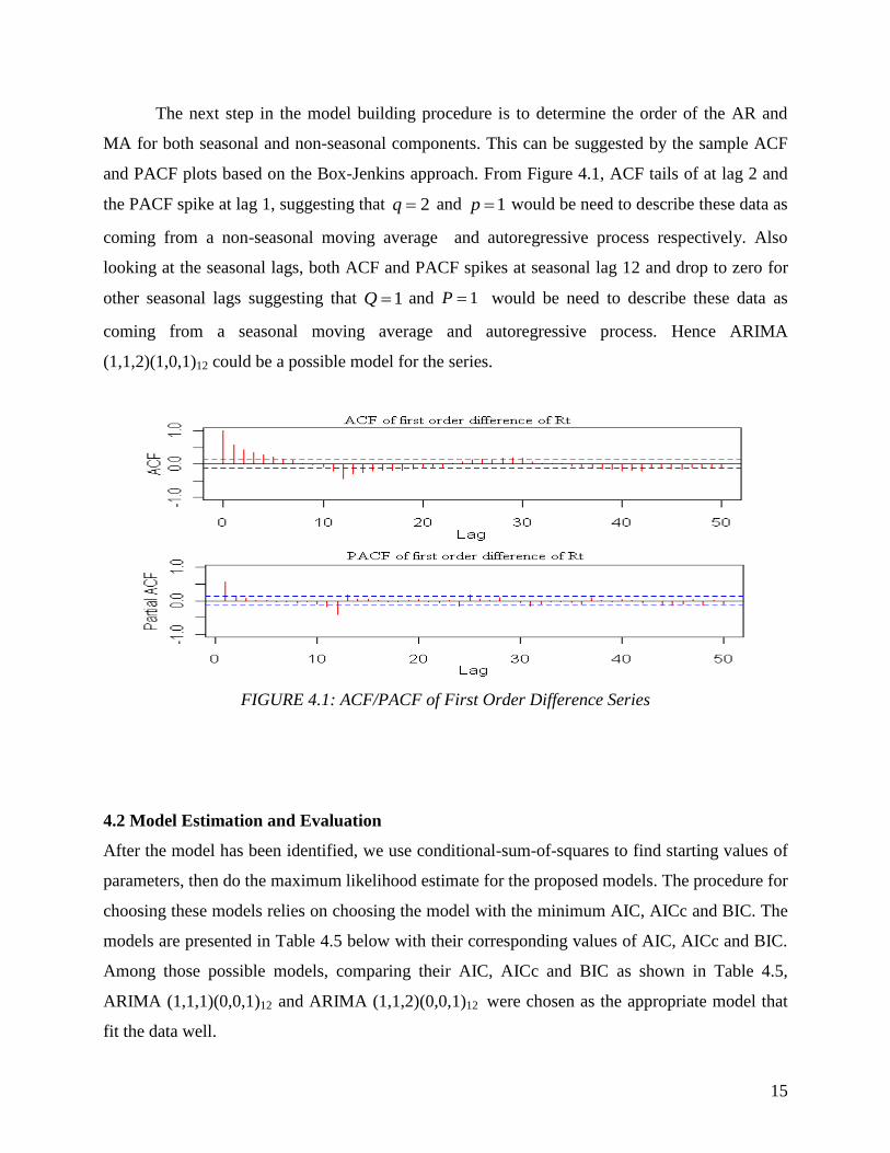
The next step in the model building procedure is to determine the order of the AR and

MA for both seasonal and non-seasonal components. This can be suggested by the sample ACF

and PACF plots based on the Box-Jenkins approach. From Figure 4.1, ACF tails of at lag 2 and

the PACF spike at lag 1, suggesting that 2q and 1p would be need to describe these data as

coming from a non-seasonal moving average and autoregressive process respectively. Also

looking at the seasonal lags, both ACF and PACF spikes at seasonal lag 12 and drop to zero for

other seasonal lags suggesting that 1Q and 1P would be need to describe these data as

coming from a seasonal moving average and autoregressive process. Hence ARIMA

(1,1,2)(1,0,1)12 could be a possible model for the series.

FIGURE 4.1: ACF/PACF of First Order Difference Series

4.2 Model Estimation and Evaluation

After the model has been identified, we use conditional-sum-of-squares to find starting values of

parameters, then do the maximum likelihood estimate for the proposed models. The procedure for

choosing these models relies on choosing the model with the minimum AIC, AICc and BIC. The

models are presented in Table 4.5 below with their corresponding values of AIC, AICc and BIC.

Among those possible models, comparing their AIC, AICc and BIC as shown in Table 4.5,

ARIMA (1,1,1)(0,0,1)12 and ARIMA (1,1,2)(0,0,1)12 were chosen as the appropriate model that

fit the data well.

16

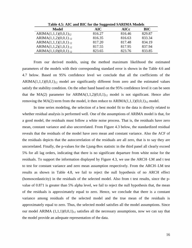
Table 4.5: AIC and BIC for the Suggested SARIMA Models

Model AIC AICc BIC

ARIMA(1,1,1)(0,0,1)12 816.27 816.46 829.87

ARIMA(1,1,2)(0,0,1) 12 816.35 816.63 833.34

ARIMA(1,1,1)(1,0,1) 12 817.20 817.48 834.19

ARIMA(1,1,2)(1,0,1) 12 817.55 817.95 837.94

ARIMA(1,1,0)(0,0,1) 12 823.65 823.76 833.85

From our derived models, using the method maximum likelihood the estimated

parameters of the models with their corresponding standard error is shown in the Table 4.6 and

4.7 below. Based on 95% confidence level we conclude that all the coefficients of the

ARIMA(1,1,1)(0,0,1)12 model are significantly different from zero and the estimated values

satisfy the stability condition. On the other hand based on the 95% confidence level it can be seen

that the MA(2) parameter for ARIMA(1,1,2)(0,0,1)12 model is not significant. Hence after

removing the MA(2) term from the model, it then reduce to ARIMA(1,1,1)(0,0,1)12 model.

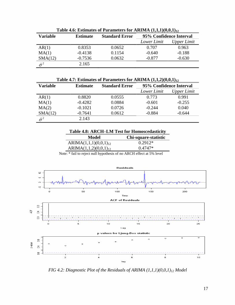
In time series modeling, the selection of a best model fit to the data is directly related to

whether residual analysis is performed well. One of the assumptions of ARIMA model is that, for

a good model, the residuals must follow a white noise process. That is, the residuals have zero

mean, constant variance and also uncorrelated. From Figure 4.3 below, the standardized residual

reveals that the residuals of the model have zero mean and constant variance. Also the ACF of

the residuals depicts that the autocorrelation of the residuals are all zero, that is to say they are

uncorrelated. Finally, the p-values for the Ljung-Box statistic in the third panel all clearly exceed

5% for all lag orders, indicating that there is no significant departure from white noise for the

residuals. To support the information displayed by Figure 4.3, we use the ARCH–LM and t test

to test for constant variance and zero mean assumption respectively. From the ARCH–LM test

results as shown in Table 4.8, we fail to reject the null hypothesis of no ARCH effect

(homoscedasticity) in the residuals of the selected model. Also from t test results, since the p-

value of 0.871 is greater than 5% alpha level, we fail to reject the null hypothesis that, the mean

of the residuals is approximately equal to zero. Hence, we conclude that there is a constant

variance among residuals of the selected model and the true mean of the residuals is

approximately equal to zero. Thus, the selected model satisfies all the model assumptions. Since

our model ARIMA (1,1,1)(0,0,1)12 satisfies all the necessary assumptions, now we can say that

the model provide an adequate representation of the data.

17

Table 4.6: Estimates of Parameters for ARIMA (1,1,1)(0,0,1)12

Variable Estimate Standard Error 95% Confidence Interval

Lower Limit Upper Limit

AR(1) 0.8353 0.0652 0.707 0.963

MA(1) -0.4138 0.1154 -0.640 -0.188

SMA(12) -0.7536 0.0632 -0.877 -0.630 2

2.165

Table 4.7: Estimates of Parameters for ARIMA (1,1,2)(0,0,1)12

Variable Estimate Standard Error 95% Confidence Interval

Lower Limit Upper Limit

AR(1) 0.8820 0.0555 0.773 0.991

MA(1) -0.4282 0.0884 -0.601 -0.255

MA(2) -0.1021 0.0726 -0.244 0.040

SMA(12) -0.7641 0.0612 -0.884 -0.644 2

2.143

Table 4.8: ARCH–LM Test for Homoscedasticity

Model Chi-square-statistic

ARIMA(1,1,1)(0,0,1)12 0.2912*

ARIMA(1,1,2)(0,0,1)12 0.4747* Note: * fail to reject null hypothesis of no ARCH effect at 5% level

FIG 4.2: Diagnostic Plot of the Residuals of ARIMA (1,1,1)(0,0,1)12 Model

18

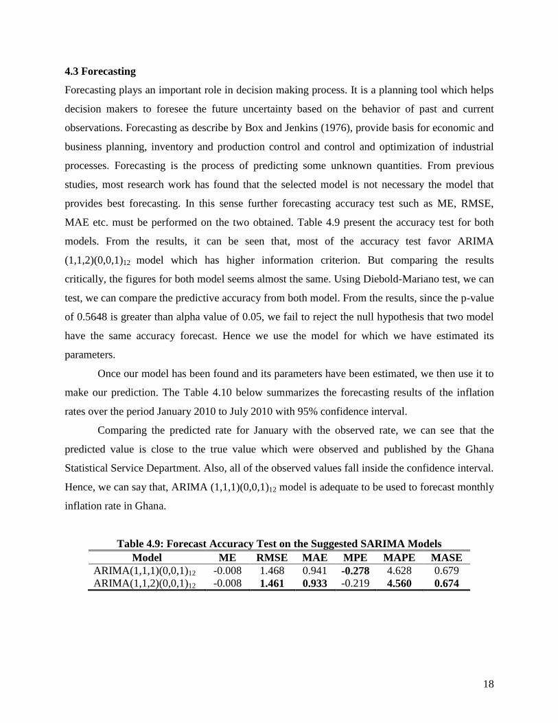
4.3 Forecasting

Forecasting plays an important role in decision making process. It is a planning tool which helps

decision makers to foresee the future uncertainty based on the behavior of past and current

observations. Forecasting as describe by Box and Jenkins (1976), provide basis for economic and

business planning, inventory and production control and control and optimization of industrial

processes. Forecasting is the process of predicting some unknown quantities. From previous

studies, most research work has found that the selected model is not necessary the model that

provides best forecasting. In this sense further forecasting accuracy test such as ME, RMSE,

MAE etc. must be performed on the two obtained. Table 4.9 present the accuracy test for both

models. From the results, it can be seen that, most of the accuracy test favor ARIMA

(1,1,2)(0,0,1)12 model which has higher information criterion. But comparing the results

critically, the figures for both model seems almost the same. Using Diebold-Mariano test, we can

test, we can compare the predictive accuracy from both model. From the results, since the p-value

of 0.5648 is greater than alpha value of 0.05, we fail to reject the null hypothesis that two model

have the same accuracy forecast. Hence we use the model for which we have estimated its

parameters.

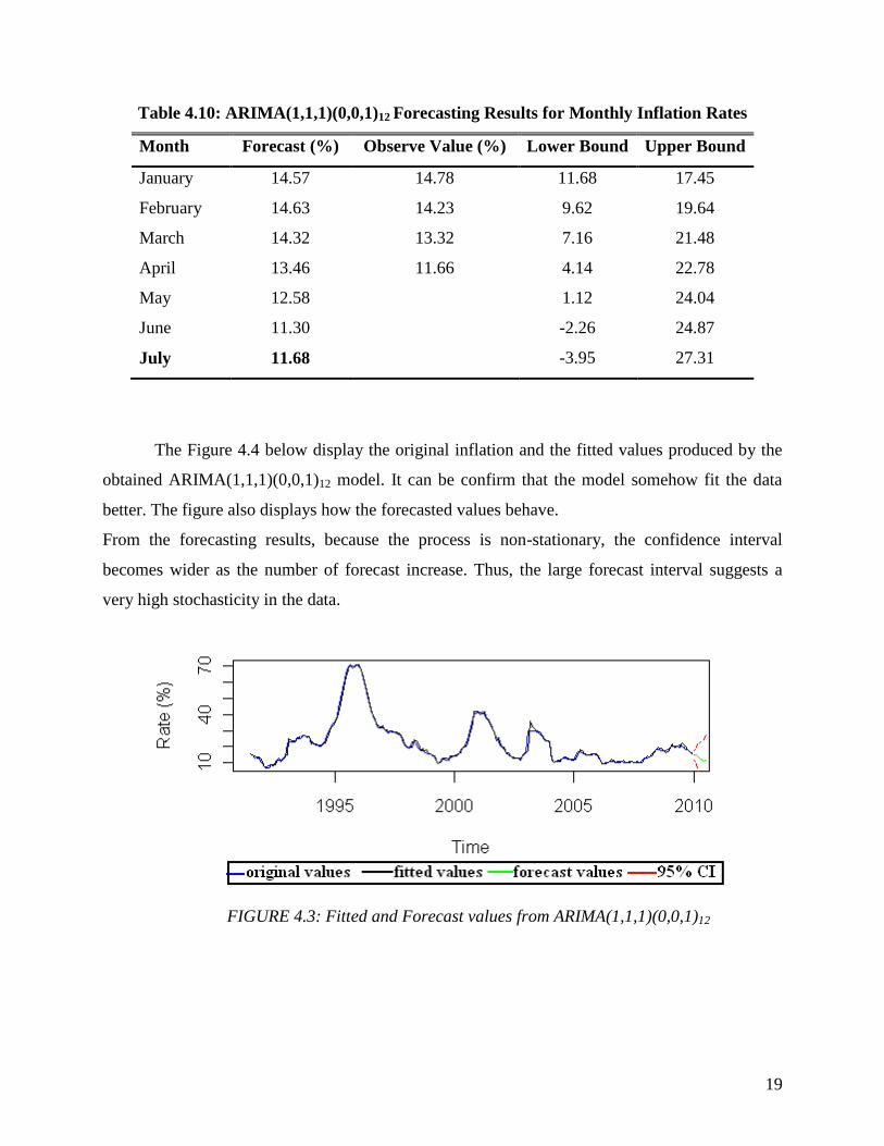
Once our model has been found and its parameters have been estimated, we then use it to

make our prediction. The Table 4.10 below summarizes the forecasting results of the inflation

rates over the period January 2010 to July 2010 with 95% confidence interval.

Comparing the predicted rate for January with the observed rate, we can see that the

predicted value is close to the true value which were observed and published by the Ghana

Statistical Service Department. Also, all of the observed values fall inside the confidence interval.

Hence, we can say that, ARIMA (1,1,1)(0,0,1)12 model is adequate to be used to forecast monthly

inflation rate in Ghana.

Table 4.9: Forecast Accuracy Test on the Suggested SARIMA Models

Model ME RMSE MAE MPE MAPE MASE

ARIMA(1,1,1)(0,0,1)12 -0.008 1.468 0.941 -0.278 4.628 0.679

ARIMA(1,1,2)(0,0,1)12 -0.008 1.461 0.933 -0.219 4.560 0.674

19

Table 4.10: ARIMA(1,1,1)(0,0,1)12 Forecasting Results for Monthly Inflation Rates

Month Forecast (%) Observe Value (%) Lower Bound Upper Bound

January 14.57 14.78 11.68 17.45

February 14.63 14.23 9.62 19.64

March 14.32 13.32 7.16 21.48

April 13.46 11.66 4.14 22.78

May 12.58 1.12 24.04

June 11.30 -2.26 24.87

July 11.68 -3.95 27.31

The Figure 4.4 below display the original inflation and the fitted values produced by the

obtained ARIMA(1,1,1)(0,0,1)12 model. It can be confirm that the model somehow fit the data

better. The figure also displays how the forecasted values behave.

From the forecasting results, because the process is non-stationary, the confidence interval

becomes wider as the number of forecast increase. Thus, the large forecast interval suggests a

very high stochasticity in the data.

FIGURE 4.3: Fitted and Forecast values from ARIMA(1,1,1)(0,0,1)12

20

5 CONCLUSION

Following the Box-Jenkins approach, Seasonal Autoregressive Integrated Moving Average

(SARIMA) was employed to analyse monthly inflation rate of Ghana from July 1991 to

December 2009. The study mainly intended to forecast the monthly inflation rate for the coming

period of January, 2010 to July 2010.

Based on minimum AIC, AICc and BIC value, the best-fitted SARIMA models tends to

be ARIMA(1,1,1)(0,0,1)12 and ARIMA(1,1,2)(0,0,1)12 model. After the estimation of the

parameters of selected model, a series of diagnostic and forecast accuracy test were performed.

Having satisfied all the model assumptions, ARIMA(1,1,1)(0,0,1)12 model was judge to be the

best model for forecasting.

The forecasting results in general revealed a decreasing pattern of inflation rate over the

forecasted period and turning point at the month of July. In light of the forecasted results, policy

makers should gain insight into more appropriate economic and monetary policy in other to

combat such increase in inflation rate which is yet to occur at the month of July.

The accuracy of forecasted future values is the core point for every forecaster. This is

because the forecasted values will affect the quality of the policies implemented based on this

forecast. With this motive, it is therefore recommend that future research on this topic is of great

concerned and it will be helpful to access the performance of the model used in this research in

terms of forecast precision as compare to other time series models. The precision of forecast does

not based on complexity or simplicity of the model used.

From the description of the Ghana inflation rates behavior, it was found that, an increase

in world oil prices always leads to increase in Ghana inflation rate. In the next few years Ghana

will be an oil producer and it is believe that if the county managed the newly found natural

resources (oil) well, then increase in world market oil price will not affect inflation in the country

so much. This will also pave way for policy makers to study inflation situation in Ghana in other

to determine other factors that contribute to high inflation rates in the country.

21

REFERNCES

[1] Adam, C., Ndulu, B. and Sowa, N.K (1996). Liberalization and Seigniorage Revenue in

Kenya, Ghana and Tanzania. The Journal of Development Studies, 32(4, April), 531–53.

[2] Aidan, M., Geoff, K. and Terry, Q. (1998). Forecasting Irish Inflation Using ARIMA

Models. CBI Technical Papers 3/RT/98:1-48, Central Bank and Financial Services

Authority of Ireland.

[3] Akaike, H.(1974). A New Look at the Statistical Model Identification. IEEE Transactions

on Automatic Controll 19 (6): 716–723.

[4] Amediku, S. (2006). Stress Test of the Ghanaian Banking Sector: A VAR Approach. BOG

Working Papers 2006/02, Bank of Ghana.

[5] Asel, I. (2007). Modeling and Forecasting Inflation in Developing Countries: The Case of

Economies in Central Asia. CERGE-EI Discussion Papers 2007-174, Center for Economic

Research and Graduate Education, Academy of Science of the Czech Republic Economic

Institute.

[6] Beaulieu, J. & Miron, J. (1993), Seasonal unit roots in aggregate U.S. data. Journal of

Econometrics, 54: 305-328.

[7] Box, G.E.P. & Jenkins, G.M. (1976) Time Series Analysis: Forecasting and Control.

Holden-Day, San Francisco.

[8] Brockwell, P. J. & Davis, R. A. (1996) Introduction to Time Series and Forecasting.

Springer, New York.

[9] Burnham, K.P., & Anderson, D.R. (1998). Model Selection and Inference. Springer-Verlag,

New York.

[10] Buss, G. (2009). Comparing forecasts of Latvia's GDP using Simple Seasonal ARIMA

models and Direct versus Indirect. MPRA Paper No. 16825, Munich Personal RePec

Archive.

[11] Canova, F & Hansen, B.E (1995), Are Seasonal Patterns Constant Over Time? A Test for

Seasonal Stability. Journal of Business and Economic Statistics, 13, 237-252.

[12] Chan, N.H (2002) Time Series Application To Finance. John Wiley & Sons, Inc., USA.

[13] Cowpertwait, P.S.P & Metcalfe, A.V. (2009) Introductory Time Series with R. Springer

Science +Business Media, LLC, NY, USA.

22

[14] Cromwell, J.B., LABYS, W.C., & Terraza M. (1994) Univariate Tests for Time Series

Models. Sage University Paper series on Quantitative Applications in the Social Sciences,

07-099. Thousand Oaks, CA: Sage.

[15] Cryer J.D & Kung-Sik C. (2008) Time Series Analysis with Applications in R. 2Ed.

Springer Science +Business Media, LLC, NY, USA.

[16] David, F.H. (2001) Modelling UK Inflation, 1875-1991. Journal of Applied Econometrics,

16(3): 255-275.

[17] De Brouwer, G. & Neil, R.E. (1998). Modelling Inflation in Australia. Journal of Business

& Economic Statistics, American Statistical Association, 16(4): 433-49.

[18] Dickey, D.A. & Fuller, W.A. (1979). Distribution of the Estimators for Autoregressive Time

Series with Unit Root. Journal of the American Statistical Association, 74: 427-431.

[19] Dickey, D.A. & Fuller, W.A. (1981). Likelihood Ratio Statistics for Autoregressive Time

Series with a Unit Root. Econometrica, 49(4), 1057-1072.

[20] Diebold, F.X. and Mariano, R.S. (1995) Comparing Predictive Accuracy. Journal of

Business and Economic Statistics, 13, 253-263.

[21] Engle, R.F (2001). GARCH 101: The Use of ARCH/GARCH Models in Applied

Econometrics", Journal of Economic Perspectives, 15(4): 157-168

[22] Fedderke, J.W. & Schaling, E. (2005). Modelling Inflation in South Africa: A Multivariate

Cointegration Analysis. South African Journal of Economics, 73(1): 79-92.

[23] Franses, P.H. (1990), Testing for Seasonal Unit Roots in Monthly Data, Technical Report

9032, Econometric Institute.

[24] Halim, S. & Bisono, I.N. (2008). Automatic Seasonal Autoregressive Moving Average

Models and Unit Root Test Detection. International Journal of Management Science and

Engineering Management, 3(4): 266-274

[25] Hall, R. (1982). Inflation, Causes and Effects. University of Chicago Press, Chicago.

[26] Hamilton, J. D. (1994). Time Series Analysis. Princeton Univ. Press, Princeton New Jersey.

[27] Hellerstein, R. (1997). “The Impact of Inflation” Regional Review, Winter 1997, 7(1).

[28] Hurvich, C.M., & Tsai, C.L (1989). Regression and Time Series Model Selection in Small

Sample. Biometrika, 76: 297-307.

[29] Hylleberg, S., Engle, R., Granger, C. & Yoo, B. (1990), Seasonal Integration and

Cointegration. Journal of Econometrics, 44: 215-238.

23

[30] Kenji, M. & Abdul N. (2009). Forecasting Inflation in Sudan. IMF Working Papers 09/132,

International Monetary Fund.

[31] Kihoro, J.M., Otieno, R.O., & Wafula, C. (2004). Seasonal Time Series Forecasting: A

Comparactive Study of ARIMA and ANN Models. African Journal of Science and

Technology, 5(2): 41-49

[32] Kirchgässner, G &Wolters, J. (2007) Introduction To Modern Time Series Analysis.

Springer-Verlag Berlin Heidelberg

[33] Kivilcim, M. (1998). The Relationship between Inflation and the Budget Deficit in Turkey.

Journal of Business and Economic Statistics, 16(4): 412-422.

[34] Kleiber, C. & Zeileis, A. (2008) Applied Econometrics with R. Springer Science +Business

Media, LLC, NY, USA.

[35] Kwiatkowski, D., Phillips, P. C. B., Schmidt, P. & Shin, Y. (1992): Testing the Null

Hypothesis of Stationarity against the Alternative of a Unit Root. Journal of Econometrics

54, 159–178.

[36] Junttila, J. (2001). Structural breaks, ARIMA Model and Finnish Inflation Forecasts

International Journal of Forecasting, 17: 203–230

[37] Mame, A.D. (2007). Modeling Inflation for Mali. IMF Working Papers 07/295,

International Monetary Fund.

[38] Ocran, M.K. (2007). A Modelling of Ghana's Inflation Experience: 1960–2003. African

Economic Research Consortium, RP_169.

[39] Michael, H.C. (1981).U.S. inflation and the import demand of Ghana and Nigeria, 1967–

1976. Journal of The Review of Black Political Economy, 11(2), 217-228.

[40] Pankratz, A. (1983) Forecasting with Univariate Box-Jenkins Models: Concepts and Cases.

John Wily & Sons. Inc. USA

[41] Pfaff, B. (2008) Analysis of Integrated and Cointegrated Time Series with R. 2Ed, Springer

Science +Business Media, LLC, NY, USA.

[42] Phillips, P.C.B. and Perron, P. (1988), Testing for a unit root in time series regression,

Biometrika, 75(2), 335–346.

[43] Pufnik, A. and Kunovac, D. (2006). Short-Term Forecasting of Inflation in Croatia with

Seasonal ARIMA Processes. Working Paper, W-16, Croatia National Bank.

24

[44] R Development Core Team (2009). R: A Language and Environment for Statistical

Computing. R Foundation for Statistical Computing, Vienna, Austria. ISBN 3-900051-07-0,

URL http://www.R-project.org.

[45] Sakamoto, Y., Ishiguro, M., and Kitagawa G. (1986). Akaike Information Criterion

Statistics. D. Reidel Publishing Company.

[46] Schulz, P.M. and Prinz, A. (2009). Forecasting Container Transshipment in Germany.

Applied Economics, 41(22): 2809-2815

[47] Schwarz, G. E. (1978). Estimating the Dimension of a Model. Annals of Statistics 6 (2):

461–464.

[48] Shumway, R.H. and Stoffer, D.S. (2006)Time Series Analysis and Its Applications With R

Examples 2Ed, Springer Science +Business Media, LLC, NY, USA.

[49] Sowa, N.K. (1996). Policy Consistency and Inflation in Ghana. African Economic Research

Consortium, RP_43.

[50] Sowa, N.K. and Kwakye, J. (1991). Inflationary Trends and Control in Ghana. African

Economic Research Consortium, RP_22.

[51] Tim, C. and Dongkoo, C. (1999). Modelling and Forecasting Inflation in India. IMF

Working Papers 99/119, International Monetary Fund

[52] Tsay, R.S. (2002) Analysis of Financial Time Series. John Wiley & Sons, Inc. USA

[53] Webster, D. (2000). Webster's New Universal Unabridged Dictionary. Barnes & Noble

Books, New York

[54] Zivot, E. and Andrews, D. W.K. (1992), Further Evidence on the Great Crash, the Oil-Price

Shock, and the Unit-Root Hypothesis, Journal of Business & Economic Statistics, 10(3),

251–270.