1 Hidden Markov Models Ronald J. Williams CSG220 Spring 2007 Contains several slides adapted from an Andrew Moore tutorial on this topic and a few figures from Russell & Norvig’s AIMA site and Alpaydin’s Introduction to Machine Learning site. Hidden Markov Models: Slide 2 A Simple Markov Chain s 2 s 3 1/3 1/3 1/3 1/3 2/3 2/3 1/3 s 1 1/2 1/2 0 Numbers at nodes represent probability of starting at the corresponding state. Numbers on arcs represent transition probabilities. At each time step, t = 1, 2, ... a new state is selected randomly according to the distribution at the current state. Let X t be a random variable for the state at time step t. Let x t represent the actual value of the state at time t. In this example, x t can be s 1 , s 2 , or s 3 .
Transcript
1
Hidden Markov Models
Ronald J. WilliamsCSG220
Spring 2007
Contains several slides adapted from an Andrew Moore tutorial on this topic and a few figures from Russell & Norvig’s AIMA site and Alpaydin’s Introduction to Machine Learning site.
Hidden Markov Models: Slide 2
A Simple Markov Chain
s2
s3
1/3
1/3
1/3
1/3
2/32/3
1/3
s11/2 1/2
0
Numbers at nodes represent probability of starting at the corresponding state.
Numbers on arcs represent transition probabilities.
At each time step, t = 1, 2, ... a new state is selected randomly according to the distribution at the current state.
Let Xt be a random variable for the state at time step t.
Let xt represent the actual value of the state at time t.In this example, xt can be s1, s2, or s3.
2
Hidden Markov Models: Slide 3
Markov Property• For any t, Xt+1 is conditionally independent of {Xt-1, Xt-2, … X1}
given Xt.
• In other words:
P(Xt+1 = sj |Xt = si ) = P(Xt+1 = sj |Xt = si ,any earlier history)
• Question: What would be the best Bayes Net structure to represent the Joint Distribution of (X1, X2, … , Xt-1, Xt, ...)?
Hidden Markov Models: Slide 4
Markov Property• For any t, Xt+1 is conditionally independent of {Xt-1, Xt-2, … X1}
given Xt.
• In other words:
P(Xt+1 = sj |Xt = si ) = P(Xt+1 = sj |Xt = si ,any earlier history)
• Question: What would be the best Bayes Net structure to represent the Joint Distribution of (X1, X2, … , Xt-1, Xt, ...)?
• Answer:
X1 X2 Xt-1 Xt. . . . . .
3
Hidden Markov Models: Slide 5
Markov chain as a Bayes netX1 X2 Xt-1 Xt
. . . . . .
aNN…aNj
…aN2aN1N
aiN…aij
…ai2ai1i
:::::::
…
…
…
…
a3Na3j…a32a31
3
a2Na2j…a22a21
2
a1Na1j…a12a11
1
Nj…21
Same CPT at every node except X1
Notation:
)(
)|(
1
1
ii
itjtij
sXP
sXsXPa
==
=== +
π
πNN
πii
π33π22π11P(X1 = si)i
Hidden Markov Models: Slide 6
Markov Chain: Formal Definition
A Markov chain is a 3-tuple consisting of• a set of N possible states {s1, s2, ..., sN}• {π1, π2, .. πN} The starting state probabilities
πi = P(X1 = si)• a11 a22 … a1N
a21 a22 … a2N
: : :aN1 aN2 … aNN
The state transition probabilities
aij = P(Xt+1=sj | Xt=si)
4
Hidden Markov Models: Slide 7
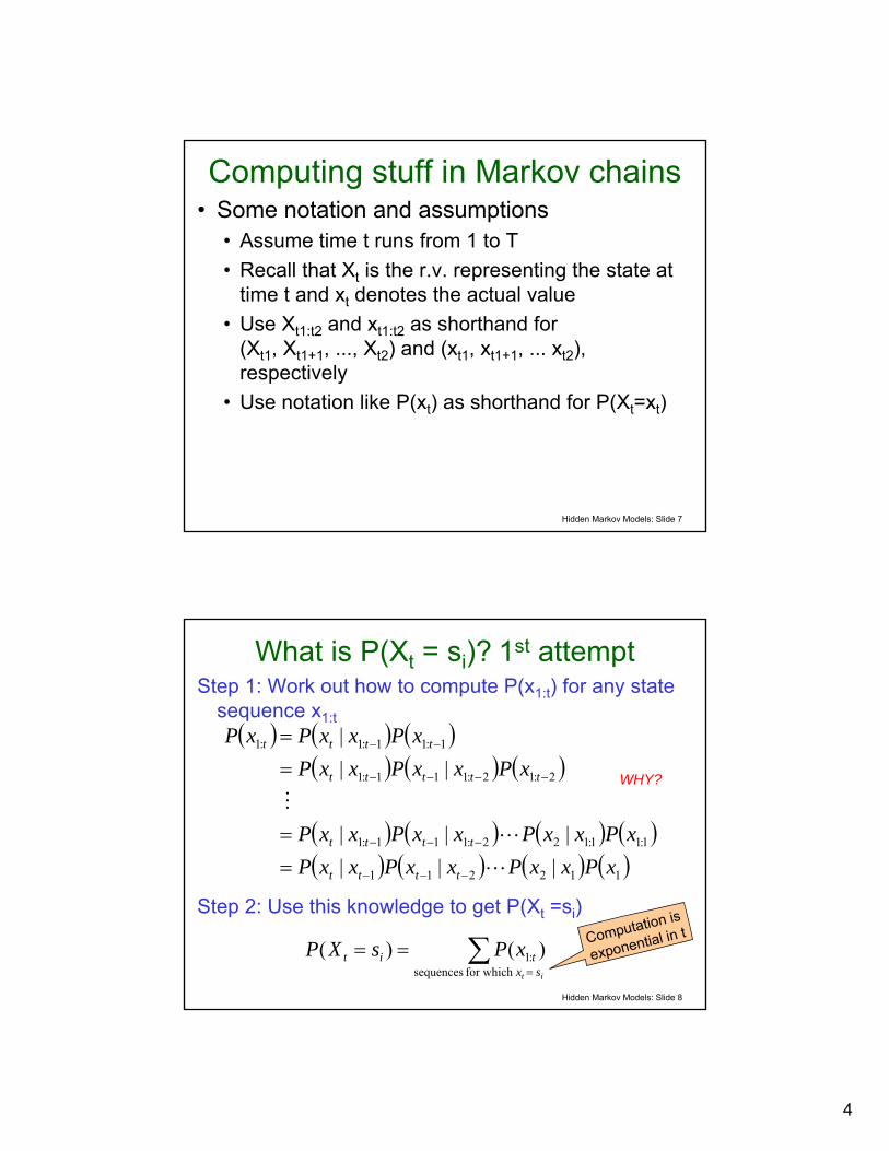
Computing stuff in Markov chains• Some notation and assumptions
• Assume time t runs from 1 to T• Recall that Xt is the r.v. representing the state at
time t and xt denotes the actual value• Use Xt1:t2 and xt1:t2 as shorthand for
(Xt1, Xt1+1, ..., Xt2) and (xt1, xt1+1, ... xt2), respectively
• Use notation like P(xt) as shorthand for P(Xt=xt)
Hidden Markov Models: Slide 8
What is P(Xt = si)? 1st attemptStep 1: Work out how to compute P(x1:t) for any state
sequence x1:t
Step 2: Use this knowledge to get P(Xt =si)
WHY?
∑=
==it sx
tit xPsXP for which sequences
:1 )()( Computation is
exponential in t
( ) ( ) ( )( ) ( ) ( )
( ) ( ) ( ) ( )( ) ( ) ( ) ( )112211
1:11:122:111:1
2:12:111:1
1:11:1:1
||||||
|||
xPxxPxxPxxPxPxxPxxPxxP
xPxxPxxPxPxxPxP
tttt
tttt
ttttt
tttt
L
L
M
−−−
−−−
−−−−
−−
==
==
5
Hidden Markov Models: Slide 9
State sequence as a path
trellis
Exponentially many paths, but at each time step only goes through exactly one of the N states
Hidden Markov Models: Slide 10
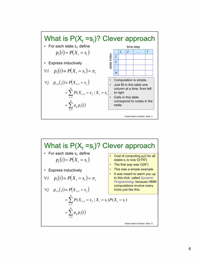
What is P(Xt =si)? Clever approach• For each state si, define
• Express inductively
( ) ( ) iisXPipi π==≡∀ 11
( ) ( )itt sXPip ==
( ) ( )
( )∑
∑
=
=+
++
=
====
=≡∀
N
itij
N
iititjt
jtt
ipa
sXPsXsXP
sXPjpj
1
11
11
)()|(
6
Hidden Markov Models: Slide 11
What is P(Xt =si)? Clever approach• For each state si, define
• Express inductively
( ) ( ) iisXPipi π==≡∀ 11
( ) ( )itt sXPip ==
( ) ( )
( )∑
∑
=
=+
++
=
====
=≡∀
N
itij
N
iititjt
jtt
ipa
sXPsXsXP
sXPjpj
1
11
11
)()|(
N
:
2
1T. . .21
time step
stat
e in
dex
• Computation is simple.• Just fill in this table one
column at a time, from left to right
• Cells in this table correspond to nodes in the trellis
Hidden Markov Models: Slide 12
What is P(Xt =si)? Clever approach• For each state si, define
• Express inductively
( ) ( ) iisXPipi π==≡∀ 11
( ) ( )itt sXPip ==
( ) ( )
( )∑
∑
=
=+
++
=
====
=≡∀
N
itij
N
iititjt
jtt
ipa
sXPsXsXP
sXPjpj
1
11
11
)()|(
• Cost of computing pt(i) for all states si is now O(TN2)
• The first way was O(NT)• This was a simple example• It was meant to warm you up
to this trick, called Dynamic Programming, because HMM computations involve many tricks just like this.
7
Hidden Markov Models: Slide 13
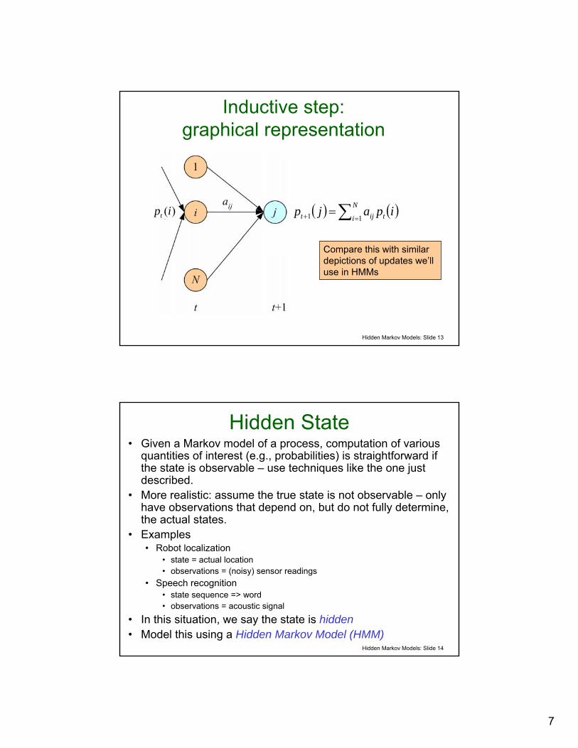
Inductive step:graphical representation
( ) ( )∑ =+ =N
i tijt ipajp11 )(ipt
Compare this with similar depictions of updates we’ll use in HMMs
Hidden Markov Models: Slide 14
Hidden State• Given a Markov model of a process, computation of various
quantities of interest (e.g., probabilities) is straightforward if the state is observable – use techniques like the one just described.
• More realistic: assume the true state is not observable – only have observations that depend on, but do not fully determine, the actual states.
• Examples• Robot localization
• state = actual location• observations = (noisy) sensor readings
• Speech recognition• state sequence => word• observations = acoustic signal
• In this situation, we say the state is hidden• Model this using a Hidden Markov Model (HMM)
8
Hidden Markov Models: Slide 15
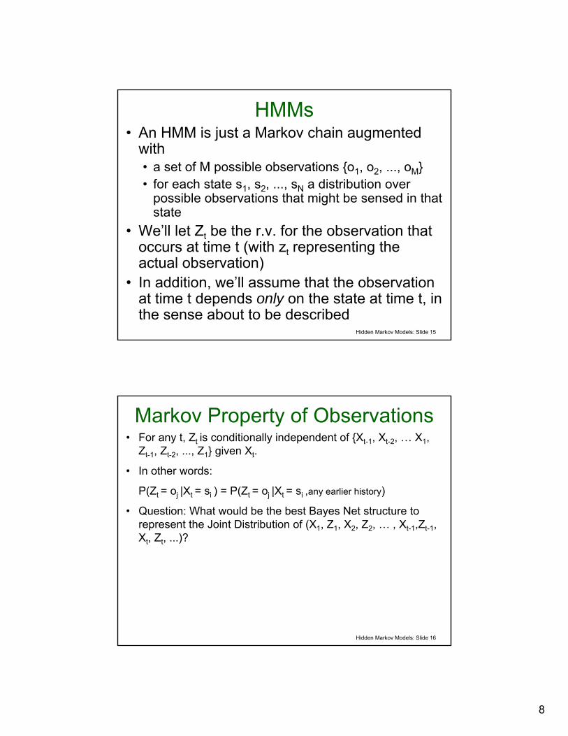
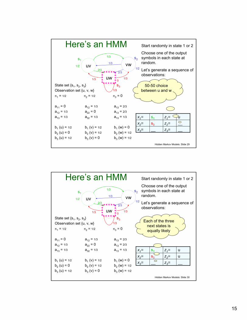
HMMs• An HMM is just a Markov chain augmented
with• a set of M possible observations {o1, o2, ..., oM}• for each state s1, s2, ..., sN a distribution over
possible observations that might be sensed in that state
• We’ll let Zt be the r.v. for the observation that occurs at time t (with zt representing the actual observation)
• In addition, we’ll assume that the observation at time t depends only on the state at time t, in the sense about to be described
Hidden Markov Models: Slide 16
Markov Property of Observations• For any t, Zt is conditionally independent of {Xt-1, Xt-2, … X1,
Zt-1, Zt-2, ..., Z1} given Xt.
• In other words:
P(Zt = oj |Xt = si ) = P(Zt = oj |Xt = si ,any earlier history)
• Question: What would be the best Bayes Net structure to represent the Joint Distribution of (X1, Z1, X2, Z2, … , Xt-1,Zt-1, Xt, Zt, ...)?
9
Hidden Markov Models: Slide 17
Markov Property of Observations• For any t, Zt is conditionally independent of {Xt-1, Xt-2, … X1,
Zt-1, Zt-2, ..., Z1} given Xt.
• In other words:
P(Zt = oj |Xt = si ) = P(Zt = oj |Xt = si ,any earlier history)
• Question: What would be the best Bayes Net structure to represent the Joint Distribution of (X1, Z1, X2, Z2, … , Xt-1,Zt-1, Xt, Zt, ...)?
• Answer:X1 X2 Xt-1 Xt
. . . . . .
Z1 Z2 Zt-1 Zt
Hidden Markov Models: Slide 18
Notation:
HMM as a Bayes NetX1 X2 Xt-1 Xt
. . . . . .
Z1 Z2 Zt-1 Zt
:::::::
bN (oM)…bN(ok)…bN (o2)bN (o1)N
bi (oM)…bi(ok)…bi (o2)bi(o1)i
:::::::
…
…
…
…
b3 (oM)b3(ok)…b3 (o2)b3 (o1)3
b2 (oM)b2(ok)…b2 (o2)b2 (o1)2
b1(oM)b1 (ok)…b1 (o2)b1(o1)1
Mk…21 This is the CPT for every Z node
)|()( itktki sXoZPob ===
observation index
stat
e in
dex
10
Hidden Markov Models: Slide 19
Are HMMs Useful?You bet !!• Robot planning & sensing under uncertainty (e.g.
Reid Simmons / Sebastian Thrun / Sven Koenig)• Robot learning control (e.g. Yangsheng Xu’s work)• Speech Recognition/Understanding
Phones → Words, Signal → phones• Human Genome Project
Complicated stuff your lecturer knows nothing about.
• Consumer decision modeling• Economics & Finance.Plus at least 5 other things I haven’t thought of.
Hidden Markov Models: Slide 20
Dynamic Bayes Nets• An HMM is actually a special case of a more
general concept: Dynamic Bayes Net (DBN)• Can decompose into multiple state variables
and multiple observation variables at each time slice, with only direct influences represented explicitly
• (1st order) Markov property: nodes in any time slice have arcs only from nodes in their own or the immediately preceding time slice
• Higher-order Markov models also easily represented in this framework
11
Hidden Markov Models: Slide 21
DBN Example
Linear dynamical system with position sensors
E.g., target tracking
Hidden Markov Models: Slide 22
Another DBN Example
Modeling a robot with position sensors and a battery charge meter
12
Hidden Markov Models: Slide 23
Back to HMMs ...Summary of our HMM notation:• Xt = state at time t (r.v.)• Zt = observation at time t (r.v.)• Vt1:t2 = (Vt1, Vt1+1, ..., Vt2) for any time-indexed r.v. V• Possible states = {s1, s2, ..., sN}• Possible observations = {o1, o2, ..., oM}• vt = actual value of r.v. V at time step t• vt1:t2 = (vt1, vt1+1, ..., vt2) = sequence of actual values
of r.v. V from time steps t1 through t2• Convenient shorthand: E.g., P(x1:t⏐z1:t) means
P(X1:t = x1:t⏐Z1:t = z1:t)• T = final time step
Hidden Markov Models: Slide 24
HMM: Formal DefinitionAn HMM λ is a 5-tuple consisting of• a set of N possible states {s1, s2, ..., sN}• a set of M possible observations {o1, o2, ..., oM}• {π1, π2, .. πN} The starting state probabilities
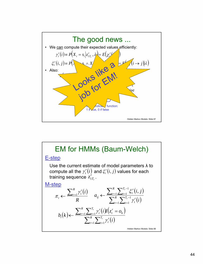
• Used especially in HMM applications:• observation sequence likelihood• most probable path• maximum likelihood model fitting
19
Hidden Markov Models: Slide 37
Filtering
X1 X2 Xt-1 Xt. . . . . .
Z1 Z2 Zt-1 Zt
current time
Xt+1
Zt+1
observed
infer (distribution)
( )λ, Compute :1 tt zXP
Hidden Markov Models: Slide 38
Prediction
...X1 X2 Xt-1 Xt... ...
Z1 Z2 Zt-1 Zt
Xk
Zk
observed
infer (distribution)current time
( ) tkzXP tk >for , Compute :1 λ
20
Hidden Markov Models: Slide 39
Smoothing
...X1 X2 Xk Xt...
Z1 Z2 Zk Zt
current time
Xt+1
Zt+1
observed
infer (distribution)
...
( ) tkzXP tk <for , Compute :1 λ
Hidden Markov Models: Slide 40
Observation Sequence Likelihood
observed
X1 X2 Xt-1 Xt. . . . . .
Z1 Z2 Zt-1 Zt
XT
ZT
What’s the probability of this particular sequence of observations as a function of the model parameters?
( )λtzP :1 Compute
Useful for such things as finding which of a set of HMM models best fits an observation sequence, as in speech recognition.
21
Hidden Markov Models: Slide 41
Most Probable Path
Not necessarily the same as the sequence of individually most probable states (obtained by smoothing)
X1 X2 Xt-1 Xt. . . . . .
Z1 Z2 Zt-1 Zt
XT
ZT
observed
infer (only most probable)
( )λ,maxarg Compute :1:1:1 TTx zxPT
Hidden Markov Models: Slide 42
Maximum Likelihood ModelAssume number of states givenGiven a set of R observation sequences
Compute
∏=
=R
r
rTr
zP1
:1* )|(maxarg λλ λ
( )( )
( )
, ,,
, ,,
, ,,
21:1
222
21
2:1
112
11
1:1
22
11
RT
RRRT
TT
TT
RRzzzz
zzzz
zzzz
K
M
K
K
=
=
=
22
Hidden Markov Models: Slide 43
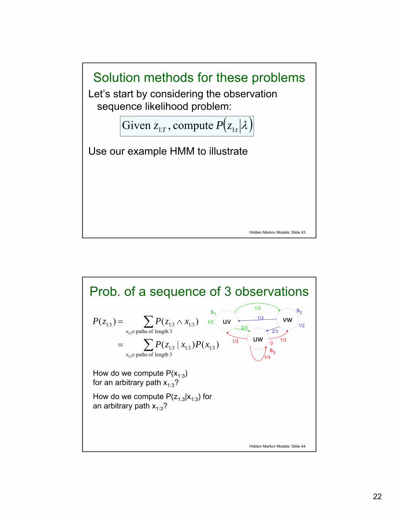
Solution methods for these problemsLet’s start by considering the observation
sequence likelihood problem:
Use our example HMM to illustrate
( )λtT zPz :1:1 compute ,Given
Hidden Markov Models: Slide 44
Prob. of a sequence of 3 observations
uv
uw
vws2s1
s3
1/3
1/3
1/3
1/3
2/32/3
1/3
1/21/2
0∑
∑
∈
∈
=
∧=
3length of paths3:13:13:1
3length of paths3:13:13:1
3:1
3:1
)()|(
)()(
x
x
xPxzP
xzPzP
How do we compute P(x1:3)for an arbitrary path x1:3?
How do we compute P(z1:3|x1:3) for an arbitrary path x1:3?
23
Hidden Markov Models: Slide 45
Prob. of a sequence of 3 observations
uv
uw
vws2s1
s3
1/3
1/3
1/3
1/3
2/32/3
1/3
1/21/2
0∑
∑
∈
∈
=
∧=
3length of paths3:13:13:1
3length of paths3:13:13:1
3:1
3:1
)()|(
)()(
x
x
xPxzP
xzPzP
How do we compute P(x1:3)for an arbitrary path x1:3?
How do we compute P(z1:3|x1:3) for an arbitrary path x1:3?
P(x1,x2,x3) = P(x1) P(x2|x1) P(x3| x2)
E.g, P(s1, s3, s3) =1/2 * 2/3 * 1/3 = 1/9
Hidden Markov Models: Slide 46
Prob. of a sequence of 3 observations
uv
uw
vws2s1
s3
1/3
1/3
1/3
1/3
2/32/3
1/3
1/21/2
0∑
∑
∈
∈
=
∧=
3length of paths3:13:13:1
3length of paths3:13:13:1
3:1
3:1
)()|(
)()(
x
x
xPxzP
xzPzP
How do we compute P(x1:3)for an arbitrary path x1:3?
How do we compute P(z1:3|x1:3) for an arbitrary path x1:3?
P(x1,x2,x3) = P(x1) P(x2|x1) P(x3| x2)
E.g, P(s1, s3, s3) =1/2 * 2/3 * 1/3 = 1/9
P(z1, z2, z3 | x1, x2, x3)
= P(z1 | x1 ) P(z2 | x2 ) P(z3 | x3 )
E.g, P(uuw | s1, s3, s3) =1/2 * 1/2 * 1/2 = 1/8
24
Hidden Markov Models: Slide 47
Prob. of a sequence of 3 observations
uv
uw
vws2s1
s3
1/3
1/3
1/3
1/3
2/32/3
1/3
1/21/2
0∑
∑
∈
∈
=
∧=
3length of paths3:13:13:1
3length of paths3:13:13:1
3:1
3:1
)()|(
)()(
x
x
xPxzP
xzPzP
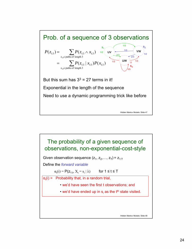
But this sum has 33 = 27 terms in it!
Exponential in the length of the sequence
Need to use a dynamic programming trick like before
Hidden Markov Models: Slide 48
The probability of a given sequence of observations, non-exponential-cost-style
Given observation sequence (z1, z2,…, zT) = z1:T
Define the forward variable
αt(i) = P(z1:t, Xt = si | λ) for 1 ≤ t ≤ T
αt(i) = Probability that, in a random trial,
• we’d have seen the first t observations; and
• we’d have ended up in si as the tth state visited.
25
Hidden Markov Models: Slide 49
( ) ( )( ) ( )
ii
ii
i
zbsXPsXzP
sXzPi
π
α
)(
1
111
111
=
===
=∧≡1
i
N
1z
1
i
N
time step 1 2
iπ
Note: For simplicity, we’ll drop explicit reference to conditioning on the HMM parameters λ for many of the upcoming slides, but it’s always there implicitly.
Base case:
Computing the forward variables
Hidden Markov Models: Slide 50
Forward variables: inductive step( ) ( )
( )( )( ) ( )( ) ( )( ) ( ) ( )
( ) ( )
( ) ( )∑∑∑∑∑∑∑
=+
= ++
+= ++
= ++
= ++
= ++
= ++
+++
=
==
===∧==
==∧=
=∧=∧=∧=
=∧=∧∧=
=∧=∧=
=∧≡
N
i tijtj
tijN
i jtt
titjtN
i itjtt
tN
i itjtt
ittN
i ittjtt
N
i jtittt
N
i jtitt
jttt
iazb
iasXzP
isXsXPsXsXzP
isXsXzP
sXzPsXzsXzP
sXsXzzP
sXsXzP
sXzPj
11
1 11
11 11
1 11
:11 :111
1 11:1
1 11:1
11:11
α
α
α
α
α sum over all possible previous states
26
Hidden Markov Models: Slide 51
Forward variables: inductive step( ) ( )
( )( )( ) ( )( ) ( )( ) ( ) ( )
( ) ( )
( ) ( )∑∑∑∑∑∑∑
=+
= ++
+= ++
= ++
= ++
= ++
= ++
+++
=
==
===∧==
==∧=
=∧=∧=∧=
=∧=∧∧=
=∧=∧=
=∧≡
N
i tijtj
tijN
i jtt
titjtN
i itjtt
tN
i itjtt
ittN
i ittjtt
N
i jtittt
N
i jtitt
jttt
iazb
iasXzP
isXsXPsXsXzP
isXsXzP
sXzPsXzsXzP
sXsXzzP
sXsXzP
sXzPj
11
1 11
11 11
1 11
:11 :111
1 11:1
1 11:1
11:11
α
α
α
α
αsplit off last observation
Hidden Markov Models: Slide 52
Forward variables: inductive step( ) ( )
( )( )( ) ( )( ) ( )( ) ( ) ( )
( ) ( )
( ) ( )∑∑∑∑∑∑∑
=+
= ++
+= ++
= ++
= ++
= ++
= ++
+++
=
==
===∧==
==∧=
=∧=∧=∧=
=∧=∧∧=
=∧=∧=
=∧≡
N
i tijtj
tijN
i jtt
titjtN
i itjtt
tN
i itjtt
ittN
i ittjtt
N
i jtittt
N
i jtitt
jttt
iazb
iasXzP
isXsXPsXsXzP
isXsXzP
sXzPsXzsXzP
sXsXzzP
sXsXzP
sXzPj
11
1 11
11 11
1 11
:11 :111
1 11:1
1 11:1
11:11
α
α
α
α
α
chain rule
27
Hidden Markov Models: Slide 53
Forward variables: inductive step( ) ( )
( )( )( ) ( )( ) ( )( ) ( ) ( )
( ) ( )
( ) ( )∑∑∑∑∑∑∑
=+
= ++
+= ++
= ++
= ++
= ++
= ++
+++
=
==
===∧==
==∧=
=∧=∧=∧=
=∧=∧∧=
=∧=∧=
=∧≡
N
i tijtj
tijN
i jtt
titjtN
i itjtt
tN
i itjtt
ittN
i ittjtt
N
i jtittt
N
i jtitt
jttt
iazb
iasXzP
isXsXPsXsXzP
isXsXzP
sXzPsXzsXzP
sXsXzzP
sXsXzP
sXzPj
11
1 11
11 11
1 11
:11 :111
1 11:1
1 11:1
11:11
α
α
α
α
α
latest state and observation conditionally independent of earlier observations given
previous state
Hidden Markov Models: Slide 54
Forward variables: inductive step( ) ( )
( )( )( ) ( )( ) ( )( ) ( ) ( )
( ) ( )
( ) ( )∑∑∑∑∑∑∑
=+
= ++
+= ++
= ++
= ++
= ++
= ++
+++
=
==
===∧==
==∧=
=∧=∧=∧=
=∧=∧∧=
=∧=∧=
=∧≡
N
i tijtj
tijN
i jtt
titjtN
i itjtt
tN
i itjtt
ittN
i ittjtt
N
i jtittt
N
i jtitt
jttt
iazb
iasXzP
isXsXPsXsXzP
isXsXzP
sXzPsXzsXzP
sXsXzzP
sXsXzP
sXzPj
11
1 11
11 11
1 11
:11 :111
1 11:1
1 11:1
11:11
α
α
α
α
α
chain rule
28
Hidden Markov Models: Slide 55
Forward variables: inductive step( ) ( )
( )( )( ) ( )( ) ( )( ) ( ) ( )
( ) ( )
( ) ( )∑∑∑∑∑∑∑
=+
= ++
+= ++
= ++
= ++
= ++
= ++
+++
=
==
===∧==
==∧=
=∧=∧=∧=
=∧=∧∧=
=∧=∧=
=∧≡
N
i tijtj
tijN
i jtt
titjtN
i itjtt
tN
i itjtt
ittN
i ittjtt
N
i jtittt
N
i jtitt
jttt
iazb
iasXzP
isXsXPsXsXzP
isXsXzP
sXzPsXzsXzP
sXsXzzP
sXsXzP
sXzPj
11
1 11
11 11
1 11
:11 :111
1 11:1
1 11:1
11:11
α
α
α
α
α
latest observation conditionally independent of earlier states given latest state
Hidden Markov Models: Slide 56
Forward variables: inductive step( ) ( )
( )( )( ) ( )( ) ( )( ) ( ) ( )
( ) ( )
( ) ( )∑∑∑∑∑∑∑
=+
= ++
+= ++
= ++
= ++
= ++
= ++
+++
=
==
===∧==
==∧=
=∧=∧=∧=
=∧=∧∧=
=∧=∧=
=∧≡
N
i tijtj
tijN
i jtt
titjtN
i itjtt
tN
i itjtt
ittN
i ittjtt
N
i jtittt
N
i jtitt
jttt
iazb
iasXzP
isXsXPsXsXzP
isXsXzP
sXzPsXzsXzP
sXsXzzP
sXsXzP
sXzPj
11
1 11
11 11
1 11
:11 :111
1 11:1
1 11:1
11:11
α
α
α
α
α
29
Hidden Markov Models: Slide 57
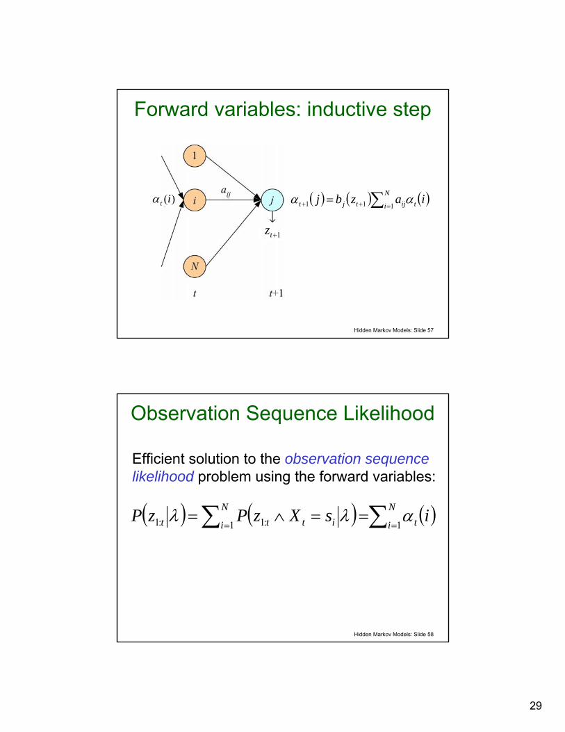
Forward variables: inductive step
1+tz
( ) ( ) ( )∑ =++ =N
i tijtjt iazbj111 αα)(itα
Hidden Markov Models: Slide 58
Observation Sequence Likelihood
Efficient solution to the observation sequence likelihood problem using the forward variables:
( ) ( ) ( )∑∑ ====∧=
N
i tN
i ittt isXzPzP11 :1:1 αλλ
30
Hidden Markov Models: Slide 59
In our example( ) ( )( ) ( )( ) ( ) ( )iazbj
zbisXzi
ti
ijtjt
ii
ittt
αα
παλα
∑++ =
=
=∧≡
11
11
:1
P
( ) ( ) ( )( ) ( ) ( )( ) ( ) ( ) 72
1312
121
721
321
2241
1
3 3 032 02 02
01 01 1
=========
ααααααααα
Observed: z1 z2 z3 = u u w
uv
uw
vws2s1
s3
1/3
1/3
1/3
1/3
2/32/3
1/3
1/21/2
0
So probability of observing uuw is 1/36
Hidden Markov Models: Slide 60
Filtering
Efficient solution to the filtering problem using the forward variables:
( ) ( )( ) ∑ =
=∧=
== N
j t
t
t
tittit
ji
zPzsXPzsXP
1:1
:1:1
)()(
αα
Estimating current state based on all observations up to the current time.
So in our example, after observing uuw, prob. of being in s1 is 0 and prob. of being in s2 = prob. of being in s3 = 1/2
31
Hidden Markov Models: Slide 61
Prediction• Note that the (state) prediction problem can
be viewed as a special case of the filtering problem in which there are missing observations.
• That is, trying to compute the probability of Xkgiven observations up through time step t, with k > t, amounts to filtering with missing observations at time steps t+1, t+2, ..., k.
• Therefore, we now focus on the missing observations problem.
Hidden Markov Models: Slide 62
Missing Observations• Looking at the derivation of the inductive step for computing the forward
variables, we see that the last step involves writing
• Thus the second factor gives us a prediction of the state at time t+1 based on all earlier observations, which we then multiply by the observation probability at time t+1 given the state at time t+1.
• If there is no observation at time t+1, clearly the set of observations made through time t+1 is the same as the set of observations made through time t.
( ) ( ) ( )tsXPsXzPj jtjttt ime through tup nsobservatio all1111 === ++++α
( ) ( )∑ =+N
i tijtj iazb11 α
32
Hidden Markov Models: Slide 63
Missing Observations (cont.)• Thus we redefine
• This generalizes our earlier definition but allows for the possibility that some observations are present and others are missing
• Then define
• It’s not hard to see that the correct forward compution should then proceed as:
• Amounts to propagating state predictions forward wherever there are no observations
• Interesting special case: When there are no observations at any time, the α values are identical to the p values we defined earlier for Markov chains
( ) ( )( ) ( ) ( )iazbj
zbi
ti
ijtjt
ii
αα
πα
∑++ ′=
′=
11
11
( ) ( )tsXPi itt ime through tnsobservatio available all∧==α
( ) ( )⎩⎨⎧=′
otherwise 1 at timen observatioan is thereif tzbzb ti
ti
Hidden Markov Models: Slide 64
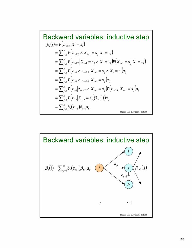
Solving the smoothing problem• Define the backward variables
• Probability of observing zt+1, ..., zT given that system was in state si at time step t
• These can be computed efficiently by starting at the end (time T) and working backwards
• Base case:• Valid because zT+1:T is an empty sequence of
observations so its probability is 1
( ) ( )λβ ,:1 itTtt sXzPi == +
( ) Ni iiT ≤≤= 1 , allfor 1β
33
Hidden Markov Models: Slide 65
Backward variables: inductive step( ) ( )
( )( ) ( )( )( )( ) ( )( ) ( )
( )∑∑∑∑∑∑∑
= ++
= +++
++= +++
= +++
= +++
= +++
= ++
+
=
==
==∧=
=∧=
=∧=∧=
===∧==
==∧=
=≡
N
j ijttj
ijN
j tjtt
ijjtTtN
j jtTtt
N
j ijjtTtt
N
j ijitjtTtt
N
j itjtitjtTt
N
j itjtTt
itTtt
azb
ajsXzP
asXzPsXzzP
asXzzP
asXsXzzP
sXsXPsXsXzP
sXsXzP
sXzPi
1 11
1 111
1:21 1:21
1 1:21
1 1:21
1 11:1
1 1:1
:1
β
β
β
Hidden Markov Models: Slide 66
Backward variables: inductive step
1+tz( )jt 1+β( ) ( )∑ = ++=
N
j ijttjt azbi1 11 ββ
34
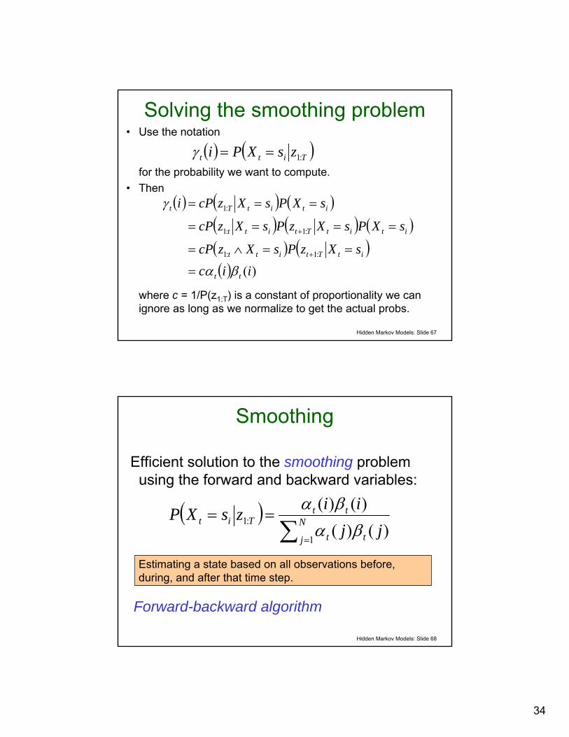
Hidden Markov Models: Slide 67
Solving the smoothing problem• Use the notation
for the probability we want to compute.• Then
where c = 1/P(z1:T) is a constant of proportionality we can ignore as long as we normalize to get the actual probs.
( ) ( )Titt zsXPi :1==γ
( ) ( ) ( )( ) ( ) ( )( ) ( )( ) )(
:1:1
:1:1
:1
iicsXzPsXzcP
sXPsXzPsXzcP
sXPsXzcPi
tt
itTtitt
ititTtitt
ititTt
βα
γ
=
==∧=
====
===
+
+
Hidden Markov Models: Slide 68
Smoothing
Efficient solution to the smoothing problem using the forward and backward variables:
( )∑ =
== N
j tt
ttTit
jjiizsXP
1
:1)()(
)()(βα
βα
Estimating a state based on all observations before, during, and after that time step.
Forward-backward algorithm
35
Hidden Markov Models: Slide 69
Solving the most probable path problem• Want• One approach:
• Easy to compute each factor for a given state and observation sequence, but number of paths is exponential in T
• Use dynamic programming instead
( )TTx zxPT :1:1:1
maxarg
( ) ( ) ( )( )
( ) ( )TTTx
T
TTTxTTx
xPxzPzP
xPxzPzxP
T
TT
:1:1:1
:1
:1:1:1:1:1
:1
:1:1
maxarg
maxargmaxarg
=
=
Hidden Markov Models: Slide 70
DP for Most Probable Path• Define
• A path giving this maximum is one of lengtht-1 having the highest probability of simultaneously• occuring• ending at si
• producing observation sequence z1:t
( ) ( )tittxt zsXxPit :11:11:1
max ∧=∧= −−δ
36
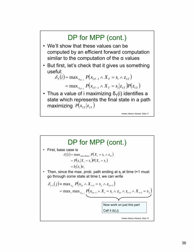
Hidden Markov Models: Slide 71
DP for MPP (cont.)• We’ll show that these values can be
computed by an efficient forward computation similar to the computation of the α values
• But first, let’s check that it gives us something useful:
• Thus a value of i maximizing δT(i) identifies a state which represents the final state in a path maximizing
( ) ( )( ) ( )TTiTTx
TiTTxT
zPzsXxP
zsXxPi
T
T
:1:11:1
:11:1
1:1
1:1
max
max
=∧=
∧=∧=
−
−
−
−δ
( )TT zxP :1:1
Hidden Markov Models: Slide 72
DP for MPP (cont.)• First, base case is
• Then, since the max. prob. path ending at sj at time t+1 must go through some state at time t, we can write
( ) ( )( ) ( )( ) ii
itit
it
zbsXPsXzP
zsXPi
π
δ
1
1
1:1choice one1 max
=
===
∧==
( ) ( )( )jtttittxi
tjttxt
sXzzsXxP
zsXxPj
t
t
=∧∧∧=∧=
∧=∧≡
++−
+++
− 11:11:1
1:11:11
1:1
:1
maxmax
maxδ
Now work on just this part
Call it Δ(i,j)
37
Hidden Markov Models: Slide 73
DP for MPP (cont.)
( ) ( )( ) ( )( ) ( )( ) ( ) ( )( ) ( )tittijtj
tittitjtjtt
tittitjtt
titttittjtt
jtttitt
zsXxPazb
zsXxPsXsXPsXzP
zsXxPsXsXzP
zsXxPzsXxsXzP
sXzzsXxPji
:11:11
:11:1111
:11:111
:11:1:11:111
11:11:1,
∧=∧=
∧=∧====
∧=∧==∧=
∧=∧∧=∧=∧=
=∧∧∧=∧≡Δ
−+
−+++
−++
−−++
++−
• Using the chain rule and the Markov property, we find that the probability to be maximized can be written as
Hidden Markov Models: Slide 74
DP for MPP (cont.)• Finally, then, we get
• This is inductive step• Virtually identical to computation of forward variables α – only
difference is that it uses max instead of sum• Also need to keep track of which state si gives max for each
state sj at the next time step to be able to determine actual MPP, not just its probability
( ) ( )( ) ( )[ ]
( ) ( )[ ]( ) ( )iazb
zsXxPazb
zsXxPazb
jij
tijitj
tittxijitj
tittijtjxi
xit
t
t
t
δ
δ
max
maxmax
maxmax
,maxmax
1
:11:11
:11:11
1
1:1
1:1
1:1
+
−+
−+
+
=
∧=∧=
∧=∧=
Δ=
−
−
−
38
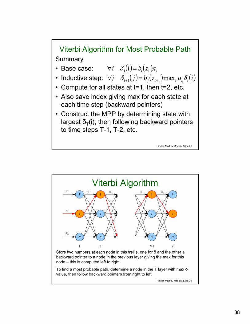
Hidden Markov Models: Slide 75
Viterbi Algorithm for Most Probable PathSummary• Base case:• Inductive step:• Compute for all states at t=1, then t=2, etc.• Also save index giving max for each state at
each time step (backward pointers)• Construct the MPP by determining state with
largest δT(i), then following backward pointers to time steps T-1, T-2, etc.
Store two numbers at each node in this trellis, one for δ and the other a backward pointer to a node in the previous layer giving the max for this node – this is computed left to right.
To find a most probable path, determine a node in the T layer with max δvalue, then follow backward pointers from right to left.
39
Hidden Markov Models: Slide 77
Viterbi algorithm: inductive step
1+tz
( ) ( ) ( )( ) ( )iaj
iazbj
tijit
tijitjt
δψ
δδ
maxarg
max
1
11
=
=
+
++)(itδ
Hidden Markov Models: Slide 78
Prob. of a given transition• The final problem we want to address is the HMM
inference (learning) problem, given a training set of observation sequences
• Most of the ingredients for deriving a max. likelihood method for this are in place
• But there’s one more sub-problem we’ll need to address:Given an observation sequence z1:T, what’s the probability that the state transition si to sj occurred at time t?
variables• Most probable path: Viterbi algorithm• Maximum likelihood model: Baum-Welch
algorithm
46
Hidden Markov Models: Slide 91
Some good references• Standard HMM reference:
L. R. Rabiner, "A Tutorial on Hidden Markov Models and Selected Applications in Speech Recognition," Proc. of the IEEE, Vol.77, No.2, pp.257-286, 1989.
• Excellent reference for Dynamic Bayes Nets as a unifying framework for probabilistic temporal models (including HMMs and Kalman filters):Chapter 15 of Artificial Intelligence, A Modern Approach, 2nd Edition, by Russell & Norvig
Hidden Markov Models: Slide 92
What You Should Know• What an HMM is• Definition, computation, and use of αt(i)• The Viterbi algorithm• Outline of the EM algorithm for HMM learning
(Baum-Welch)• Be comfortable with the kind of math needed
to derive the HMM algorithms described here• What a DBN is and how an HMM is a special