Hidden Markov Models (HMM) and Probabilistic Graphical Models...

Professor Joongheon Kim (CSE@CAU)http://sites.google.com/site/joongheon

Artificial Intelligent Lectures for Communication andNetwork Engineers/Researchers (14 April 2017)

Hidden Markov Models (HMM) and Probabilistic Graphical Models (PGM)

Professor Joongheon Kim

School of Computer Science and Engineering, Chung-Ang University, Seoul, Republic of Korea

1



Hidden Markov Models (HMM) and Probabilistic Graphical Models (PGM)Part 1: Hidden Markov Models



2



Outline

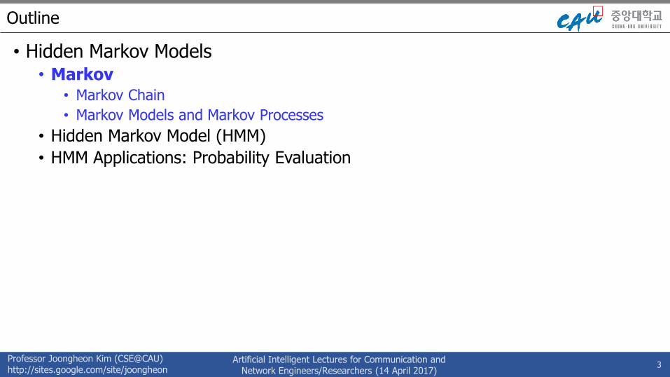
• Hidden Markov Models• Markov

• Markov Chain

• Markov Models and Markov Processes

• Hidden Markov Model (HMM)

• HMM Applications: Probability Evaluation

3



Markov (Markov Chain)

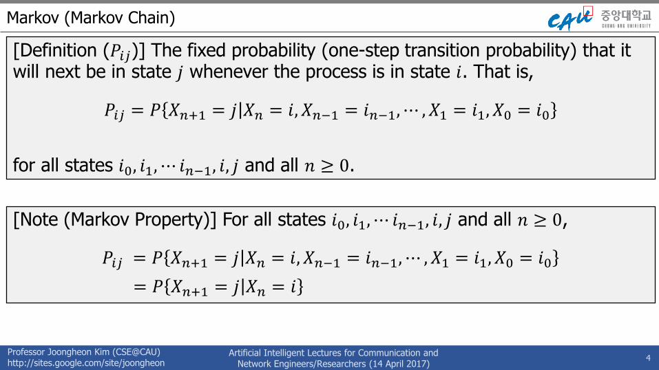
[Definition (𝑃𝑖𝑗)] The fixed probability (one-step transition probability) that it will next be in state 𝑗 whenever the process is in state 𝑖. That is,

𝑃𝑖𝑗 = 𝑃 𝑋𝑛+1 = 𝑗 𝑋𝑛 = 𝑖, 𝑋𝑛−1 = 𝑖𝑛−1, ⋯ , 𝑋1 = 𝑖1, 𝑋0 = 𝑖0

for all states 𝑖0, 𝑖1, ⋯ 𝑖𝑛−1, 𝑖, 𝑗 and all 𝑛 ≥ 0.

[Note (Markov Property)] For all states 𝑖0, 𝑖1, ⋯ 𝑖𝑛−1, 𝑖, 𝑗 and all 𝑛 ≥ 0,

𝑃𝑖𝑗 = 𝑃 𝑋𝑛+1 = 𝑗 𝑋𝑛 = 𝑖, 𝑋𝑛−1 = 𝑖𝑛−1, ⋯ , 𝑋1 = 𝑖1, 𝑋0 = 𝑖0

= 𝑃 𝑋𝑛+1 = 𝑗 𝑋𝑛 = 𝑖

4



[Markov Chain]


[Note]

• 𝑃𝑖𝑗 ≥ 0 where 𝑖 ≥ 0, 𝑗 ≥ 0

• 𝑗=0∞ 𝑃𝑖𝑗 = 1 for all 𝑖 = 0,1,⋯

5

𝑖

1

2

𝑛

⋯

𝑃𝑖1

𝑃𝑖2

𝑃𝑖𝑛

𝑃𝑖𝑖




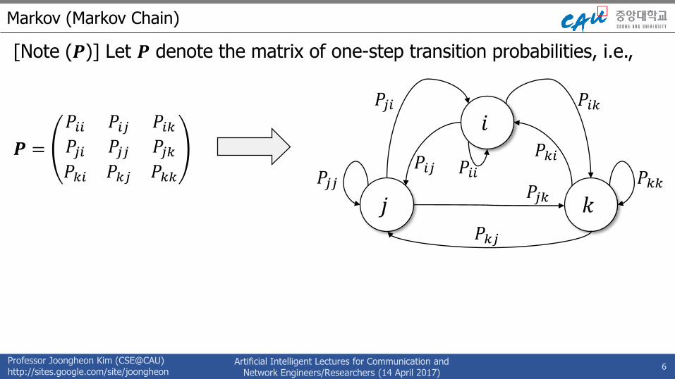
[Note (𝑷)] Let 𝑷 denote the matrix of one-step transition probabilities, i.e.,

𝑷 =

𝑃𝑖𝑖 𝑃𝑖𝑗 𝑃𝑖𝑘𝑃𝑗𝑖 𝑃𝑗𝑗 𝑃𝑗𝑘𝑃𝑘𝑖 𝑃𝑘𝑗 𝑃𝑘𝑘

6

𝑗

𝑖

𝑘

𝑃𝑖𝑖𝑃𝑖𝑗

𝑃𝑖𝑘𝑃𝑗𝑖

𝑃𝑗𝑗𝑃𝑗𝑘

𝑃𝑘𝑖

𝑃𝑘𝑗

𝑃𝑘𝑘



[Transition Matrix] [Markov Chain]


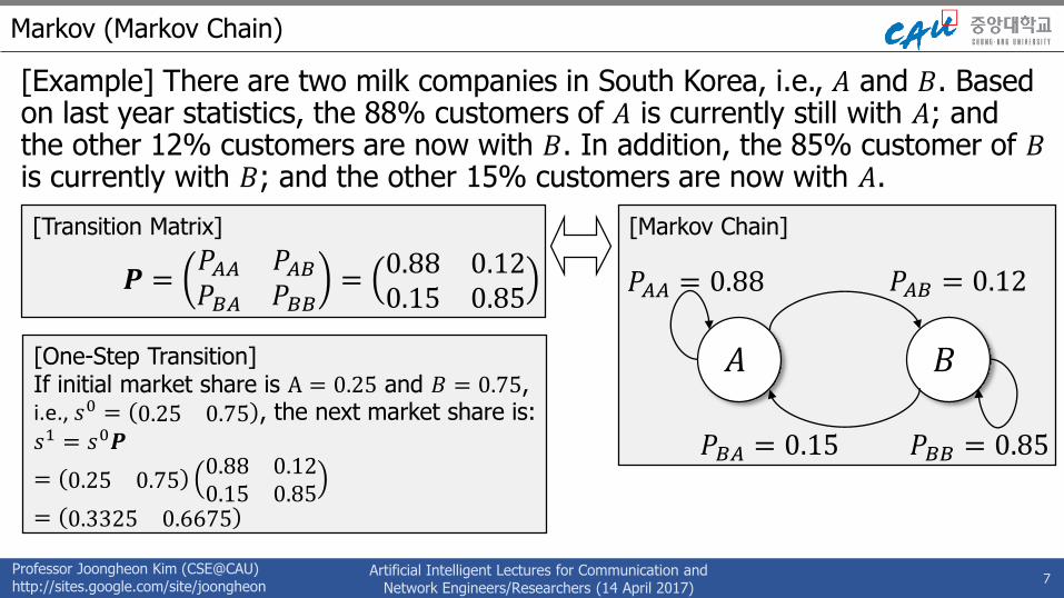
[Example] There are two milk companies in South Korea, i.e., 𝐴 and 𝐵. Based on last year statistics, the 88% customers of 𝐴 is currently still with 𝐴; and the other 12% customers are now with 𝐵. In addition, the 85% customer of 𝐵is currently with 𝐵; and the other 15% customers are now with 𝐴.

7

𝑷 =𝑃𝐴𝐴 𝑃𝐴𝐵𝑃𝐵𝐴 𝑃𝐵𝐵

=0.88 0.120.15 0.85

𝐵𝐴

𝑃𝐴𝐴 = 0.88 𝑃𝐴𝐵 = 0.12

𝑃𝐵𝐴 = 0.15 𝑃𝐵𝐵 = 0.85

[One-Step Transition]If initial market share is A = 0.25 and 𝐵 = 0.75,i.e., 𝑠0 = 0.25 0.75 , the next market share is:

𝑠1 = 𝑠0𝑷

= 0.25 0.750.88 0.120.15 0.85

= 0.3325 0.6675




[Example (Multi-Step Transition)] From the 𝑷 (in previous slide), suppose that we are in state 𝑖 in time 𝑡 and we have to compute the probability for being in state 𝑖 in time 𝑡 + 2 (denote by 𝑃𝑖𝑖

2).

8

𝑗𝑖

𝑘

𝑖

𝑖

𝑡 𝑡 + 1 𝑡 + 2

𝑃𝑖𝑖

𝑃𝑖𝑘

𝑃𝑖𝑗

𝑃𝑖𝑖

𝑃𝑗𝑖

𝑃𝑘𝑖

𝑃𝑖𝑖2 = 𝑃 𝑋𝑛+2 = 𝑖 𝑋𝑛 = 𝑖

= 𝑃𝑖𝑖𝑃𝑖𝑖 + 𝑃𝑖𝑗𝑃𝑗𝑖 + 𝑃𝑖𝑘𝑃𝑘𝑖

=



= 𝑷𝑖𝑖2

[𝑋𝑛 = 𝑖: State in 𝑖 in time 𝑛]



Markov (Markov Models and Markov Processes)

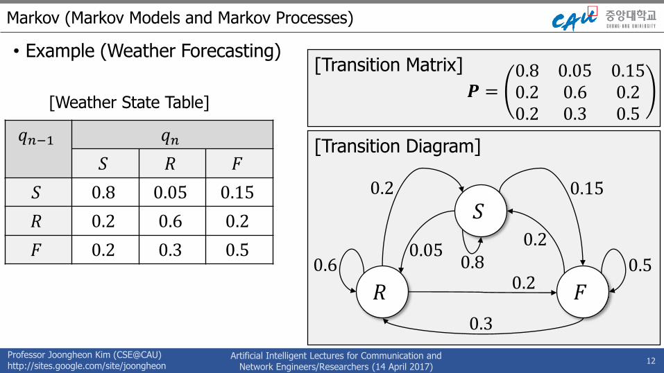
• Example for Markov Model (Weather Forecasting)• Weather State: Sunny (𝑆), Rainy (𝑅), Foggy (𝐹)

• Today’s weather 𝑞𝑛 depends on previous weather conditions, i.e., 𝑞𝑛−1, 𝑞𝑛−2, ⋯ , 𝑞1:

𝑃 𝑞𝑛 𝑞𝑛−1, 𝑞𝑛−2, ⋯ , 𝑞1

• Example: if the previous three weather conditions are 𝑞𝑛−1 = 𝑆,𝑞𝑛−2 = 𝑅, and𝑞𝑛−3 = 𝐹, subsequently, the probability where today weather (𝑞𝑛) is 𝑅 is as follows:

9

𝑃 𝑞𝑛 = 𝑅 𝑞𝑛−1 = 𝑆, 𝑞𝑛−2 = 𝑅, 𝑞𝑛−3 = 𝐹




• Observation from previous [Example]• If we have larger 𝑛, it means we have to gather more information.

• If 𝑛 = 6, we need to gather 3(6−1) = 243 weather data. Therefore, we need an assumption (called Markov Assumption) which reduces the number of gathering data.

• [First-Order Markov Assumption]

• [Second-Order Markov Assumption]

10

𝑃 𝑞𝑛 = 𝑆𝑗 𝑞𝑛−1 = 𝑆𝑖 , 𝑞𝑛−2 = 𝑆𝑘 , ⋯ = 𝑃 𝑞𝑛 = 𝑆𝑗 𝑞𝑛−1 = 𝑆𝑖

𝑃 𝑞1, 𝑞2, ⋯ , 𝑞𝑛 =

𝑖=1

𝑛

𝑃 𝑞𝑖 𝑞𝑖−1




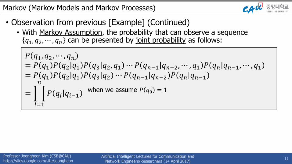
• Observation from previous [Example] (Continued)• With Markov Assumption, the probability that can observe a sequence 𝑞1, 𝑞2, ⋯ , 𝑞𝑛 can be presented by joint probability as follows:

11

𝑃 𝑞1, 𝑞2, ⋯ , 𝑞𝑛= 𝑃 𝑞1 𝑃 𝑞2 𝑞1 𝑃 𝑞3 𝑞2, 𝑞1 ⋯𝑃 𝑞𝑛−1 𝑞𝑛−2, ⋯ , 𝑞1 𝑃 𝑞𝑛 𝑞𝑛−1, ⋯ , 𝑞1= 𝑃 𝑞1 𝑃 𝑞2 𝑞1 𝑃 𝑞3 𝑞2 ⋯𝑃 𝑞𝑛−1 𝑞𝑛−2 𝑃 𝑞𝑛 𝑞𝑛−1

=

𝑖=1

𝑛

𝑃 𝑞𝑖 𝑞𝑖−1when we assume 𝑃 𝑞0 = 1



[Transition Matrix]


• Example (Weather Forecasting)

12

𝑞𝑛−1 𝑞𝑛

𝑆 𝑅 𝐹

𝑆 0.8 0.05 0.15

𝑅 0.2 0.6 0.2

𝐹 0.2 0.3 0.5

[Weather State Table]𝑷 =0.8 0.05 0.150.2 0.6 0.20.2 0.3 0.5

[Transition Diagram]

𝑅

𝑆

𝐹

0.80.05

0.150.2

0.60.2

0.2

0.3

0.5




• Example (Weather Forecasting)• Case Study: Suppose that yesterday (𝑞1)’s weather is Sunny (𝑆). Then, find the

probabilities where today (𝑞2)’s weather is Sunny (𝑆) and tomorrow (𝑞3)’s weather is Rainy (𝑅).

• (Solutions)

13

𝑃 𝑞2 = 𝑆, 𝑞3 = 𝑅 𝑞1 = 𝑆= 𝑃 𝑞3 = 𝑅 𝑞2 = 𝑆, 𝑞1 = 𝑆 ∙ 𝑃 𝑞2 = 𝑆 𝑞1 = 𝑆= 𝑃 𝑞3 = 𝑅 𝑞2 = 𝑆 ∙ 𝑃 𝑞2 = 𝑆 𝑞1 = 𝑆= 0.05 ∙ 0.8 = 0.04

[Markov Assumption]

𝑃 𝑞1 = 𝑆, 𝑞2 = 𝑆, 𝑞3 = 𝑅= 𝑃 𝑞1 = 𝑆 ∙ 𝑃 𝑞2 = 𝑆 𝑞1 = 𝑆 ∙ 𝑃 𝑞3 = 𝑅 𝑞2 = 𝑆, 𝑞1 = 𝑆= 𝑃 𝑞1 = 𝑆 ∙ 𝑃 𝑞2 = 𝑆 𝑞1 = 𝑆 ∙ 𝑃 𝑞3 = 𝑅 𝑞2 = 𝑆= 1.0 ∙ 0.8 ∙ 0.05 = 0.04

[Markov Assumption]



Outline


• Hidden Markov Model (HMM)• Example: Weather

• Example: Balls in Jars


14



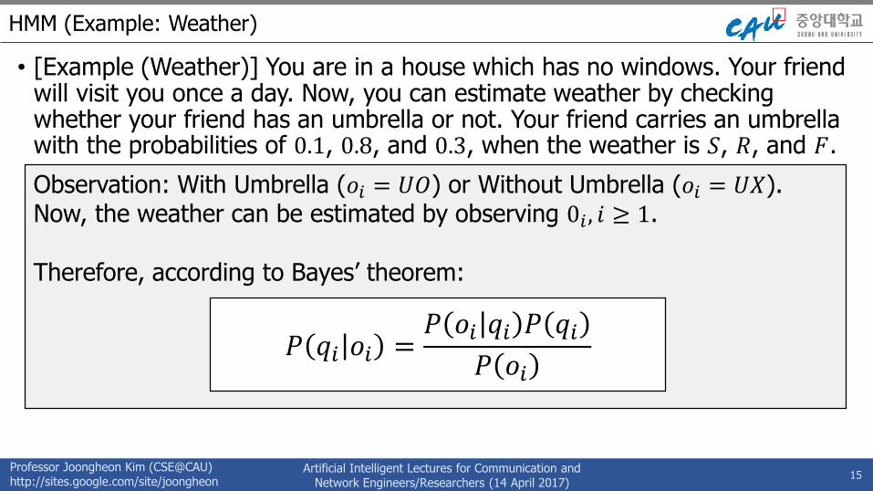
HMM (Example: Weather)

• [Example (Weather)] You are in a house which has no windows. Your friend will visit you once a day. Now, you can estimate weather by checking whether your friend has an umbrella or not. Your friend carries an umbrella with the probabilities of 0.1, 0.8, and 0.3, when the weather is 𝑆, 𝑅, and 𝐹.

15

Observation: With Umbrella (𝑜𝑖 = 𝑈𝑂) or Without Umbrella (𝑜𝑖 = 𝑈𝑋).Now, the weather can be estimated by observing 0𝑖 , 𝑖 ≥ 1.

Therefore, according to Bayes’ theorem:

𝑃 𝑞𝑖 𝑜𝑖 =𝑃 𝑜𝑖 𝑞𝑖 𝑃 𝑞𝑖𝑃 𝑜𝑖



HMM (Example: Weather)

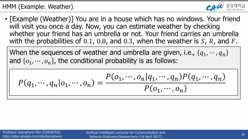
• [Example (Weather)] You are in a house which has no windows. Your friend will visit you once a day. Now, you can estimate weather by checking whether your friend has an umbrella or not. Your friend carries an umbrella with the probabilities of 0.1, 0.8, and 0.3, when the weather is 𝑆, 𝑅, and 𝐹.

16

When the sequences of weather and umbrella are given, i.e., 𝑞1, ⋯ , 𝑞𝑛and 𝑜1, ⋯ , 𝑜𝑛 , the conditional probability is as follows:

𝑃 𝑞1, ⋯ , 𝑞𝑛 𝑜1, ⋯ , 𝑜𝑛 =𝑃 𝑜1, ⋯ , 𝑜𝑛 𝑞1, ⋯ , 𝑞𝑛 𝑃 𝑞1, ⋯ , 𝑞𝑛

𝑃 𝑜1, ⋯ , 𝑜𝑛



HMM (Example: Balls in Jars)

• [Example (Weather)] A room has a curtain and there are three jars and the jars contain balls (colors: red, blue, green, and purple). A person behind the curtain select one jar and pick one ball from there. The person shows the ball and put the ball into the jar. And the person repeats.

17

Notations) • 𝑏𝑗 𝑘 : pick one ball from jar 𝑗 and the color of the ball is 𝑘 where 𝑘 = 1,2,3,4

when the color is red, blue, green, and purple, respectively.• 𝑁: The number of states (i.e., the number of jars): 𝑆 = 𝑆1, ⋯ , 𝑆𝑁• 𝑀: The number of observation (i.e., the number of colors): 𝑂 = 𝑂1, ⋯ , 𝑂𝑀• State Transition Matrix 𝐴 = 𝑎𝑖𝑗 where 𝑎𝑖𝑗 = 𝑃 𝑞𝑡+1 = 𝑆𝑗 𝑞𝑡 = 𝑆𝑖 and this

stands for the case where transition happens from state 𝑖 to state 𝑗.

• Observation 𝐵 = 𝑏𝑗 𝑘 where 𝑏𝑗 𝑘 = 𝑃 𝑂𝑡 = 𝑜𝑘 𝑞𝑡 = 𝑆𝑗 and this stands for

the case where 𝑘 is observed in state 𝑗.• Initial State Distribution 𝜋 = 𝜋𝑖 where 𝜋𝑖 = 𝑃 𝑞1 = 𝑆1 .



Outline


• Hidden Markov Model (HMM)


18



HMM Applications: Probability Evaluation

[Problem Definition (Probability Evaluation)] When 𝑂 = 𝑜1, 𝑜2, 𝑜3, ⋯ and HMM model 𝜆 = 𝐴, 𝐵, 𝜋 are given, find that the observation sequence can occur from which model with the highest probability? It means that how we can calculate 𝑃 𝑂 𝜆 ?

[Example] We are about to toss a coin with HMM model 𝜆 = 𝐴, 𝐵, 𝜋 ; and we want to find the probability of the case where observation is 𝑂 = 𝑇,𝐻, 𝑇 .

19




[Problem Definition (Probability Evaluation)] When 𝑂 = 𝑜1, 𝑜2, 𝑜3, ⋯ and HMM model 𝜆 = 𝐴, 𝐵, 𝜋 are given, find that the observation sequence can occur from which model with the highest probability? It means that how we can calculate 𝑃 𝑂 𝜆 ?

[Example] We toss a coin with HMM model 𝜆 = 𝐴, 𝐵, 𝜋 ; and we want to find the probability of the case where observation sequence is 𝑂 = 𝑇,𝐻, 𝑇 . The given HMM model 𝜆 = 𝐴, 𝐵, 𝜋 is as follows:

20

𝜋 =1

3

1

3

1

3𝐴 =

1

3

1

3

1

3

01

2

1

20 0 1

𝐵 =

1 01

2

1

21

3

2

3




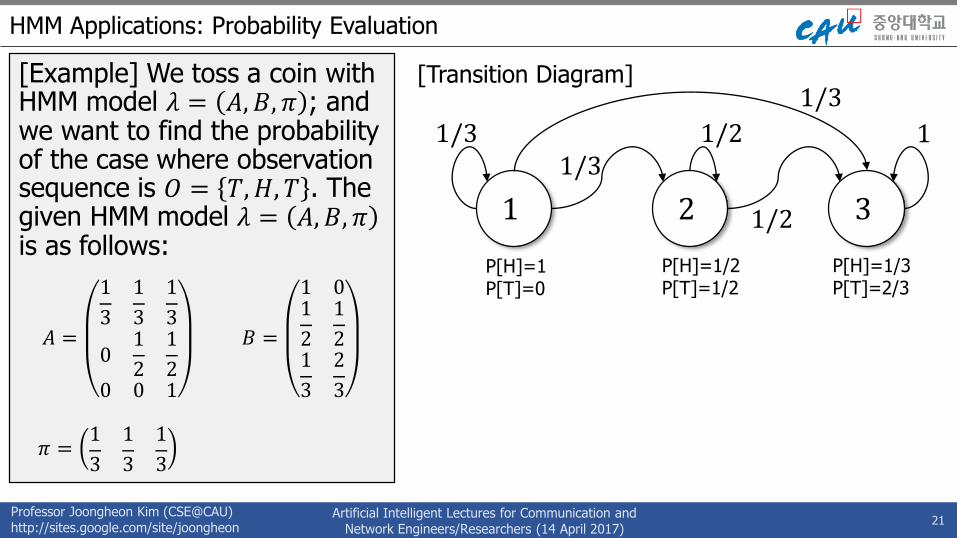
[Example] We toss a coin with HMM model 𝜆 = 𝐴, 𝐵, 𝜋 ; and we want to find the probability of the case where observation sequence is 𝑂 = 𝑇,𝐻, 𝑇 . The given HMM model 𝜆 = 𝐴, 𝐵, 𝜋is as follows:

21

𝜋 =1

3

1

3

1

3

𝐴 =

1

3

1

3

1

3

01

2

1

20 0 1

𝐵 =

1 01

2

1

21

3

2

3

21

1/3[Transition Diagram]

3

1/31/3

1/2 1

1/2

P[H]=1P[T]=0

P[H]=1/2P[T]=1/2

P[H]=1/3P[T]=2/3




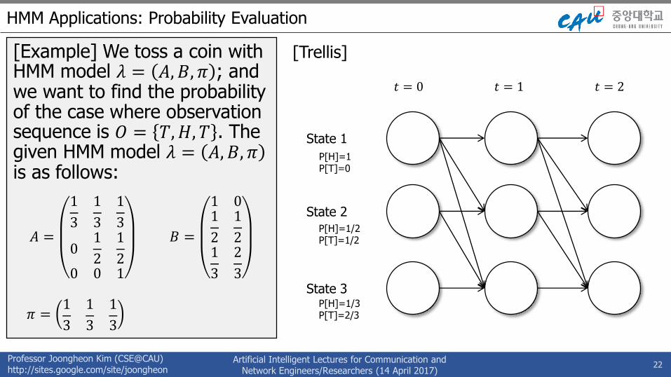
[Example] We toss a coin with HMM model 𝜆 = 𝐴, 𝐵, 𝜋 ; and we want to find the probability of the case where observation sequence is 𝑂 = 𝑇,𝐻, 𝑇 . The given HMM model 𝜆 = 𝐴, 𝐵, 𝜋is as follows:

22

𝜋 =1

3

1

3

1

3

𝐴 =

1

3

1

3

1

3

01

2

1

20 0 1

𝐵 =

1 01

2

1

21

3

2

3

[Trellis]

State 1

State 2

State 3

𝑡 = 0 𝑡 = 1 𝑡 = 2

P[H]=1P[T]=0

P[H]=1/2P[T]=1/2

P[H]=1/3P[T]=2/3




23

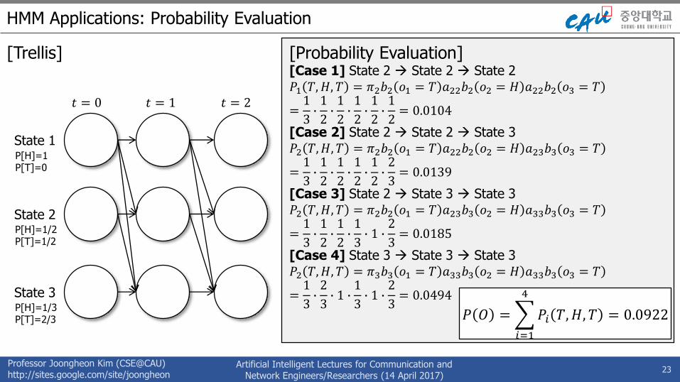
[Trellis]

State 1

State 2

State 3

𝑡 = 0 𝑡 = 1 𝑡 = 2

P[H]=1P[T]=0

P[H]=1/2P[T]=1/2

P[H]=1/3P[T]=2/3

[Probability Evaluation][Case 1] State 2 State 2 State 2𝑃1 𝑇, 𝐻, 𝑇 = 𝜋2𝑏2 𝑜1 = 𝑇 𝑎22𝑏2 𝑜2 = 𝐻 𝑎22𝑏2 𝑜3 = 𝑇

=1

3∙1

2∙1

2∙1

2∙1

2∙1

2= 0.0104

[Case 2] State 2 State 2 State 3𝑃2 𝑇,𝐻, 𝑇 = 𝜋2𝑏2 𝑜1 = 𝑇 𝑎22𝑏2 𝑜2 = 𝐻 𝑎23𝑏3 𝑜3 = 𝑇

=1

3∙1

2∙1

2∙1

2∙1

2∙2

3= 0.0139


=1

3∙1

2∙1

2∙1

3∙ 1 ∙2

3= 0.0185


=1

3∙2

3∙ 1 ∙1

3∙ 1 ∙2

3= 0.0494

𝑃 𝑂 =

𝑖=1

4

𝑃𝑖 𝑇,𝐻, 𝑇 = 0.0922




• Forward Algorithm for Probability Evaluation• Step 1) Initialization (𝛼1 𝑖 = 𝜋𝑖𝑏𝑖 𝑜𝑖 , 1 ≤ 𝑖 ≤ 3)

24

𝑡 = 0 𝑖 = 1𝛼1 1 = 𝜋1𝑏1 𝑜1 = 𝑇 =

1

3∙ 0 = 0

𝑖 = 2𝛼1 2 = 𝜋2𝑏2 𝑜1 = 𝑇 =

1

3∙1

2=1

6

𝑖 = 3𝛼1 3 = 𝜋3𝑏3 𝑜1 = 𝑇 =

1

3∙2

3=2

9

State 1

State 2

State 3

P[H]=1P[T]=0

P[H]=1/2P[T]=1/2

P[H]=1/3P[T]=2/3

𝑡 = 0 𝑡 = 1 𝑡 = 2




• Forward Algorithm for Probability Evaluation

• Step 2) Derivation (𝛼𝑡+1 𝑗 = 𝑖=13 𝛼𝑡 𝑖 𝑎𝑖𝑗 𝑏𝑖 𝑜𝑡+1 , 1 ≤ 𝑡 ≤ 2,1 ≤ 𝑗 ≤ 3)

25

𝑡 = 1 𝑗 = 1𝛼2 1 =

𝑖=1

3

𝛼1 𝑖 𝑎𝑖1 𝑏1 𝑜2 = 𝐻

= 0

𝑗 = 2𝛼2 2 =

𝑖=1

3

𝛼1 𝑖 𝑎𝑖2 𝑏2 𝑜2 = 𝐻

=1

6∙1

2∙1

2=1

24= 0.0417

𝑗 = 3𝛼2 3 =

𝑖=1

3

𝛼1 𝑖 𝑎𝑖3 𝑏3 𝑜2 = 𝐻

=1

6∙1

2+2

9∙ 1 ∙1

3= 0.1019

State 1

State 2

State 3

P[H]=1P[T]=0

P[H]=1/2P[T]=1/2

P[H]=1/3P[T]=2/3

𝑡 = 0 𝑡 = 1 𝑡 = 2




• Forward Algorithm for Probability Evaluation

• Step 2) Derivation (𝛼𝑡+1 𝑗 = 𝑖=13 𝛼𝑡 𝑖 𝑎𝑖𝑗 𝑏𝑖 𝑜𝑡+1 , 1 ≤ 𝑡 ≤ 2,1 ≤ 𝑗 ≤ 3)

26

𝑡 = 2 𝑗 = 1𝛼3 1 =

𝑖=1

3

𝛼2 𝑖 𝑎𝑖1 𝑏1 𝑜3 = 𝑇

= 0

𝑗 = 2𝛼3 2 =

𝑖=1

3

𝛼2 𝑖 𝑎𝑖2 𝑏2 𝑜3 = 𝑇

= 0.0417 ∙1

2∙1

2= 0.0104

𝑗 = 3𝛼3 3 =

𝑖=1

3

𝛼2 𝑖 𝑎𝑖3 𝑏3 𝑜3 = 𝑇

= 0.0417 ∙1

2+ 0.1019 ∙ 1 ∙

2

3= 0. 0818

State 1

State 2

State 3

P[H]=1P[T]=0

P[H]=1/2P[T]=1/2

P[H]=1/3P[T]=2/3

𝑡 = 0 𝑡 = 1 𝑡 = 2




• Forward Algorithm for Probability Evaluation• Step 2) Termination (𝑃 𝑂 𝜆 = 𝑖=1

3 𝛼3 𝑖 )

27

State 1

State 2

State 3

P[H]=1P[T]=0

P[H]=1/2P[T]=1/2

P[H]=1/3P[T]=2/3

𝑡 = 0 𝑡 = 1 𝑡 = 2

𝑃 𝑂 𝜆 = 𝑖=1

3

𝛼3 𝑖 = 0.0922



Hidden Markov Models (HMM) and Probabilistic Graphical Models (PGM)Part 2: Markov Decision Process



28



Outline

• Markov Decision Process (MDP)• Basics

• Markov Property

• Policy and Return

• Value Functions (V, Q)

• Solving MDP• Planning

• Reinforcement Learning (Value-based)

• Reinforcement Learning (Policy-based) advanced topic (out of scope)

29



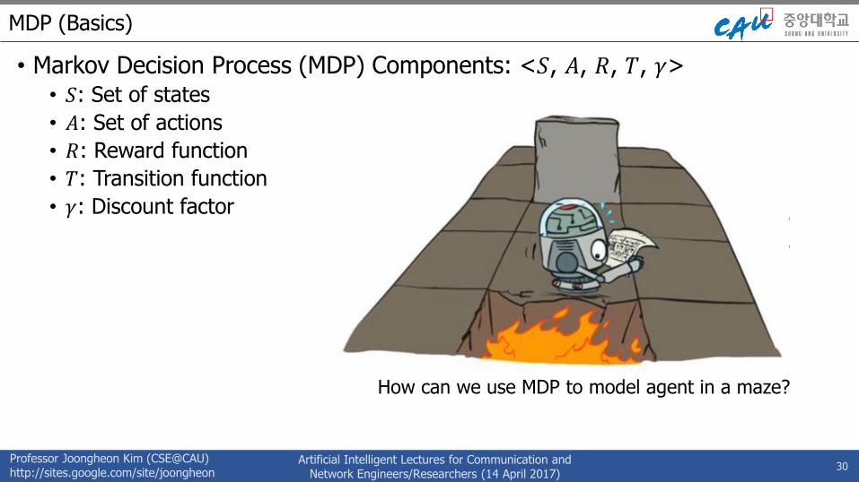
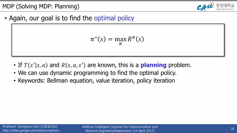
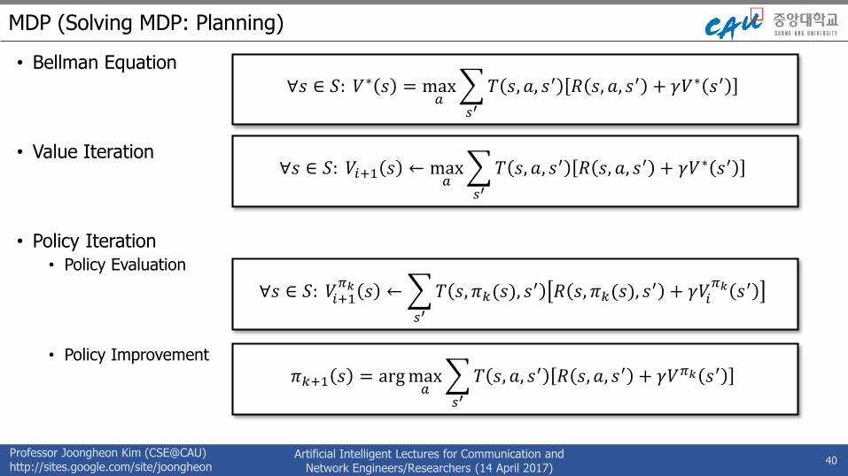
MDP (Basics)

• Markov Decision Process (MDP) Components: <𝑆, 𝐴, 𝑅, 𝑇, 𝛾>• 𝑆: Set of states

• 𝐴: Set of actions

• 𝑅: Reward function

• 𝑇: Transition function

• 𝛾: Discount factor

30

How can we use MDP to model agent in a maze?



MDP (Basics)

• Markov Decision Process (MDP) Components: <𝑆, 𝐴, 𝑅, 𝑇, 𝛾>• 𝑺: Set of states





31

𝑆: location (𝑥, 𝑦) if the maze is a 2D grid• 𝑠0: starting state• 𝑠: current state• 𝑠′: next state• 𝑠𝑡: state at time 𝑡



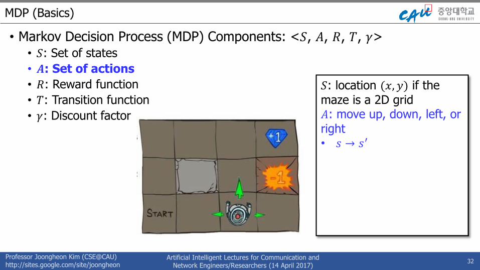
MDP (Basics)


• 𝑨: Set of actions




32

𝑆: location (𝑥, 𝑦) if the maze is a 2D grid𝐴: move up, down, left, or

right• 𝑠 → 𝑠′



MDP (Basics)



• 𝑹: Reward function



33


right𝑅: how good was the chosen action?• 𝑟 = 𝑅 𝑠, 𝑎, 𝑠′

• -1 for moving (battery used)

• +1 for jewel? +100 for exit?



MDP (Basics)




• 𝑻: Transition function


34


right𝑅: how good was the chosen action?𝑇: where is the robot’s new location?• 𝑇 = 𝑠′ 𝑠, 𝑎

Stochastic Transition



MDP (Basics)





• 𝜸: Discount factor

35

𝑆: location (𝑥, 𝑦) if the maze is a 2D grid𝐴: move up, down, left, or right𝑅: how good was the chosen action?𝑇: where is the robot’s new location?𝛾: how much does future reward worth? • 0 ≤ 𝛾 ≤ 1, [𝛾 ≈ 0: future

reward is near 0 (immediate action is preferred)]



MDP (Markov Property)

• Does 𝑠𝑡+1 depend on 𝑠0, 𝑠1, ⋯ , 𝑠𝑡−1, 𝑠𝑡 ? No.• Memoryless!

• Future only depends on present

• Current state is a sufficient statistic of agent’s history

• No need to remember agent’s history• 𝑠𝑡+1 depends only on 𝑠𝑡 and 𝑎𝑡• 𝑟𝑡 depends only on 𝑠𝑡 and 𝑎𝑡

36



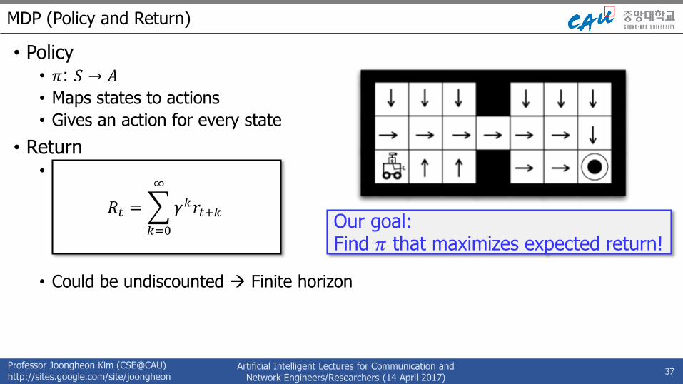
MDP (Policy and Return)

• Policy• 𝜋: 𝑆 → 𝐴

• Maps states to actions

• Gives an action for every state

• Return• Discounted sum of rewards

• Could be undiscounted Finite horizon

37

𝑅𝑡 =

𝑘=0

∞

𝛾𝑘𝑟𝑡+𝑘Our goal:Find 𝜋 that maximizes expected return!



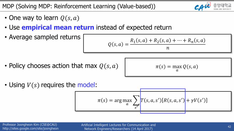
MDP (Value Functions (V, Q))

• State Value Function (𝑉)

• Expected return of starting at state 𝑠 and following policy 𝜋• How much return do I expect starting from state 𝑠?

• Action Value Function (𝑄)

• Expected return of starting at state 𝑠, taking action 𝑎, and then following policy 𝜋• How much return do I expect starting from state 𝑠 and taking action 𝑎?

38

𝑉𝜋 𝑠 = 𝐸𝜋 𝑅𝑡 𝑠𝑡 = 𝑠 = 𝐸𝜋 𝑘=0∞ 𝛾𝑘𝑟𝑡+𝑘 𝑠𝑡 = 𝑠

𝑄𝜋 𝑠, 𝑎 = 𝐸𝜋 𝑅𝑡 𝑠𝑡 = 𝑠, 𝑎𝑡 = 𝑎 = 𝐸𝜋 𝑘=0∞ 𝛾𝑘𝑟𝑡+𝑘 𝑠𝑡 = 𝑠, 𝑎𝑡 = 𝑎



MDP (Solving MDP: Planning)

• Again, our goal is to find the optimal policy

• If 𝑇 𝑠′ 𝑠, 𝑎 and 𝑅 𝑠, 𝑎, 𝑠′ are known, this is a planning problem.

• We can use dynamic programming to find the optimal policy.

• Keywords: Bellman equation, value iteration, policy iteration

39

𝜋∗ 𝑠 = max𝜋𝑅𝜋 𝑠



MDP (Solving MDP: Planning)

• Bellman Equation

• Value Iteration

• Policy Iteration

• Policy Evaluation

• Policy Improvement

40

∀𝑠 ∈ 𝑆: 𝑉∗ 𝑠 = max𝑎

𝑠′

𝑇 𝑠, 𝑎, 𝑠′ 𝑅 𝑠, 𝑎, 𝑠′ + 𝛾𝑉∗ 𝑠′

∀𝑠 ∈ 𝑆: 𝑉𝑖+1 𝑠 ← max𝑎

𝑠′

𝑇 𝑠, 𝑎, 𝑠′ 𝑅 𝑠, 𝑎, 𝑠′ + 𝛾𝑉∗ 𝑠′

∀𝑠 ∈ 𝑆: 𝑉𝑖+1𝜋𝑘 𝑠 ←

𝑠′

𝑇 𝑠, 𝜋𝑘(𝑠), 𝑠′ 𝑅 𝑠, 𝜋𝑘(𝑠), 𝑠

′ + 𝛾𝑉𝑖𝜋𝑘 𝑠′

𝜋𝑘+1 𝑠 = argmax𝑎

𝑠′

𝑇 𝑠, 𝑎, 𝑠′ 𝑅 𝑠, 𝑎, 𝑠′ + 𝛾𝑉𝜋𝑘 𝑠′



MDP (Solving MDP: Reinforcement Learning (Value-based))

• If 𝑇 𝑠′ 𝑠, 𝑎 and 𝑅 𝑠, 𝑎, 𝑠′ are unknown, this is a reinforcement learningproblem.

• Agent need to interact with the world and gather experience

• At each time-step,

• From state 𝑠

• Take action 𝑎 (𝑎 = 𝜋(𝑠) if stochastic)

• Receive reward 𝑟

• End in state 𝑠′

• Value-based: learn an optimal value function from these data

41



MDP (Solving MDP: Reinforcement Learning (Value-based))

• One way to learn 𝑄(𝑠, 𝑎)

• Use empirical mean return instead of expected return

• Average sampled returns

• Policy chooses action that max 𝑄(𝑠, 𝑎)

• Using 𝑉(𝑠) requires the model:

42

𝑄 𝑠, 𝑎 =𝑅1 𝑠, 𝑎 + 𝑅2 𝑠, 𝑎 + ⋯+ 𝑅𝑛 𝑠, 𝑎

𝑛

𝜋(𝑠) = max𝑎𝑄(𝑠, 𝑎)

𝜋 𝑠 = argmax𝑎

𝑠′

𝑇 𝑠, 𝑎, 𝑠′ 𝑅 𝑠, 𝑎, 𝑠′ + 𝛾𝑉 𝑠′



Hidden Markov Models (HMM) and Probabilistic Graphical Models (PGM)Part 3: Probabilistic Graphical Models



43



Outline

• Brief Introduction to Probabilistic Graphical Models (PGM)• What Is a Graphical Model?

• Three Key Problems• Representation

• Learning

• Inference

44



What Is a Graphical Model?

• A way of representing probabilistic relationships between random variables

• Nodes: random variables

• Edges: statistical dependencies btw these variables• Undirected edges simply give correlations between variables (Markov Random

Field or Undirected Graphical model)

• Directed edges give causality relationships (Bayesian Network or Directed Graphical Model)

• Research on Graphical Models: Multivariate Statistics + Data Structure

45



Three Key Problems

• [Representing] Represent the world as a collection of random variables 𝑋1, ⋯ , 𝑋𝑛 with joint distribution, i.e., 𝑃 𝑋1, ⋯ , 𝑋𝑛

• [Learning] Learn the distribution from data

• [Inferencing] Perform interference (i.e., compute conditional distributions), i.e., 𝑃 𝑋𝑖 𝑋1 = 𝑥1, ⋯ , 𝑋𝑛 = 𝑥𝑛

46



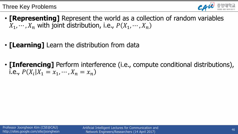
Three Key Problems

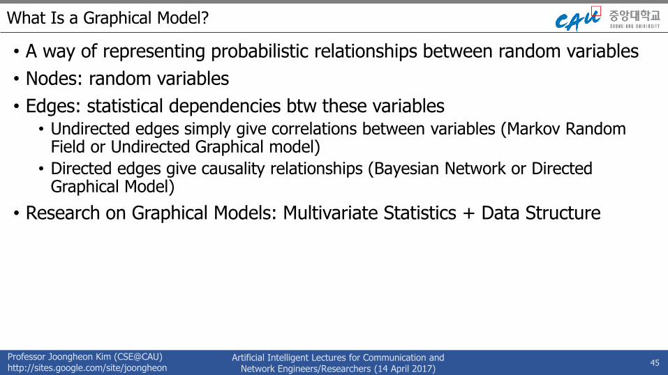
• [Representing] Represent the world as a collection of random variables 𝑋1, ⋯ , 𝑋𝑛 with joint distribution, i.e., 𝑃 𝑋1, ⋯ , 𝑋𝑛• Basics of graph theory

• Families of probability distributions

• Markov properties and conditional independence

• Density estimation, classification and regression

47



Three Key Problems

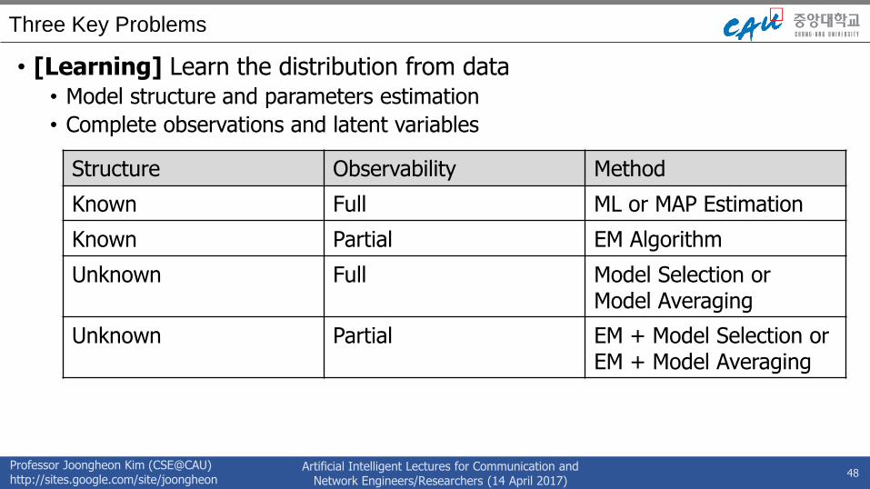
• [Learning] Learn the distribution from data• Model structure and parameters estimation

• Complete observations and latent variables

48

Structure Observability Method

Known Full ML or MAP Estimation

Known Partial EM Algorithm

Unknown Full Model Selection orModel Averaging

Unknown Partial EM + Model Selection or EM + Model Averaging



Three Key Problems

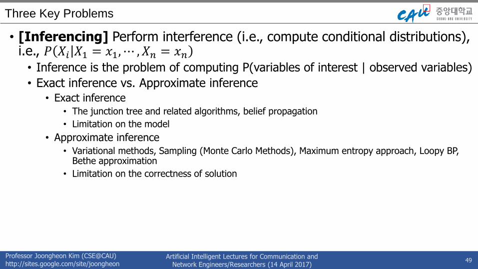
• [Inferencing] Perform interference (i.e., compute conditional distributions), i.e., 𝑃 𝑋𝑖 𝑋1 = 𝑥1, ⋯ , 𝑋𝑛 = 𝑥𝑛• Inference is the problem of computing P(variables of interest | observed variables)

• Exact inference vs. Approximate inference • Exact inference

• The junction tree and related algorithms, belief propagation

• Limitation on the model

• Approximate inference

• Variational methods, Sampling (Monte Carlo Methods), Maximum entropy approach, Loopy BP, Bethe approximation

• Limitation on the correctness of solution

49



Hidden Markov Models (HMM) and Probabilistic Graphical Models (PGM)Part 4: Support Vector Machine



50



Outline

• Main Idea

• Hyperplane in 𝑛-Dimensional Space

• Brief Introduction to Optimization for Support Vector Machine (SVM)

• SVM for Classification

51



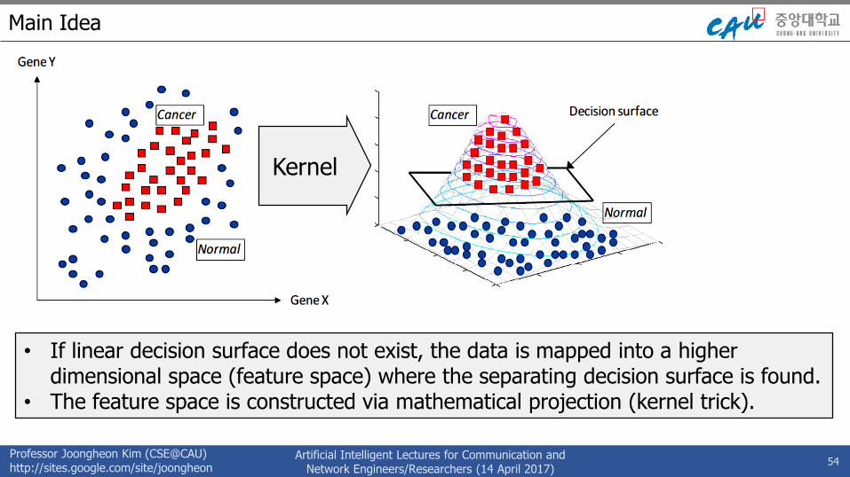
Main Idea

• How can we classify the give data?

52

Any of these would be fine. But which is the best?



Main Idea

53

Gene Y

Gene XCancer PatientsNormal Patients

Gap

Find a linear decision surface (hyperplane) that can separate patient classes and has the largest distance (i.e., largest gap (or margin)) between border-line patients (i.e., support vectors);



Main Idea

54

Kernel

• If linear decision surface does not exist, the data is mapped into a higher dimensional space (feature space) where the separating decision surface is found.

• The feature space is constructed via mathematical projection (kernel trick).



Outline

• Main Idea

• Hyperplane in 𝒏-Dimensional Space



55



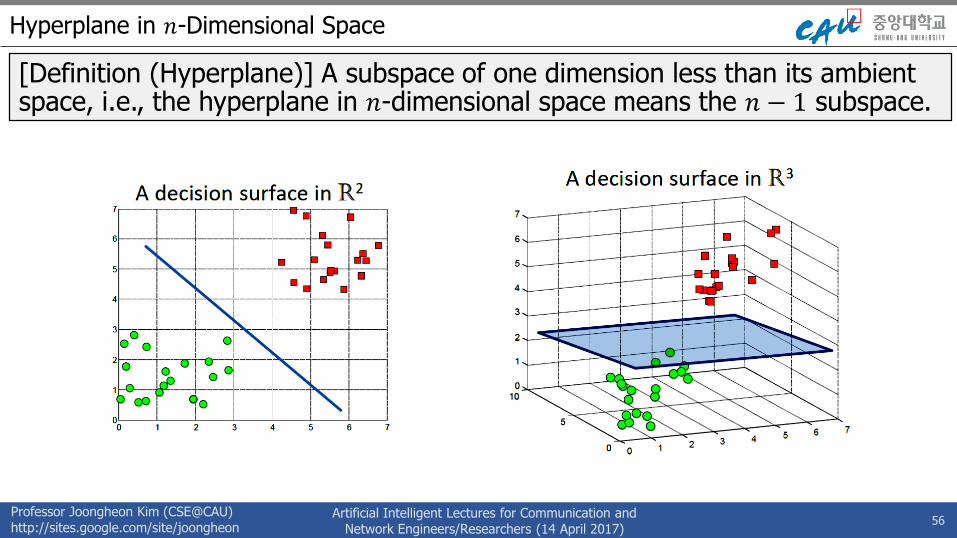
Hyperplane in 𝑛-Dimensional Space

[Definition (Hyperplane)] A subspace of one dimension less than its ambient space, i.e., the hyperplane in 𝑛-dimensional space means the 𝑛 − 1 subspace.

56




• Equations of a Hyperplane

57

• An equation of a hyperplane is defined by a point (𝑃0) and a perpendicular vector to the plane (𝑤) at that point.

• Define vectors: 𝑥0 and 𝑥 where 𝑃 is an arbitrary point on a hyperplane.

• A condition for 𝑃 to be one the plane is that the vector 𝑥 − 𝑥0 is perpendicular to 𝑤:

• The above equations hold for 𝑅𝑛 when 𝑛 > 3.

𝑤 ∙ 𝑥 − 𝑥0 = 0

𝑤 ∙ 𝑥 − 𝑤 ∙ 𝑥0 = 0 and define 𝑏 = −𝑤 ∙ 𝑥0

𝑤 ∙ 𝑥 + 𝑏 = 0

• Distance between two parallel hyperplanes 𝑤 ∙ 𝑥 +𝑏1 = 0 and 𝑤 ∙ 𝑥 + 𝑏2 = 0 is

equivalent to 𝐷 =𝑏1−𝑏2

𝑤.




• Equations of a Hyperplane

58

𝑥2 = 𝑥1 + 𝑡𝑤𝐷 = 𝑡𝑤 = 𝑡 𝑤𝑤 ∙ 𝑥2 + 𝑏2 = 0𝑤 ∙ 𝑥1 + 𝑡𝑤 + 𝑏2 = 0𝑤 ∙ 𝑥1 + 𝑡 𝑤

2 + 𝑏2 = 0𝑤 ∙ 𝑥1 + 𝑏1 − 𝑏1 + 𝑡 𝑤

2 + 𝑏2 = 0−𝑏1 + 𝑡 𝑤

2 + 𝑏2 = 0𝑡 = 𝑏1 − 𝑏2 / 𝑤

2

Therefore, 𝐷 = 𝑡 𝑤 = 𝑏1 − 𝑏2 / 𝑤

Distance between two parallel hyperplanes 𝑤 ∙ 𝑥 +𝑏1 = 0 and 𝑤 ∙ 𝑥 + 𝑏2 = 0 is equivalent to

𝐷 =𝑏1−𝑏2

𝑤.



Outline

• Main Idea




59



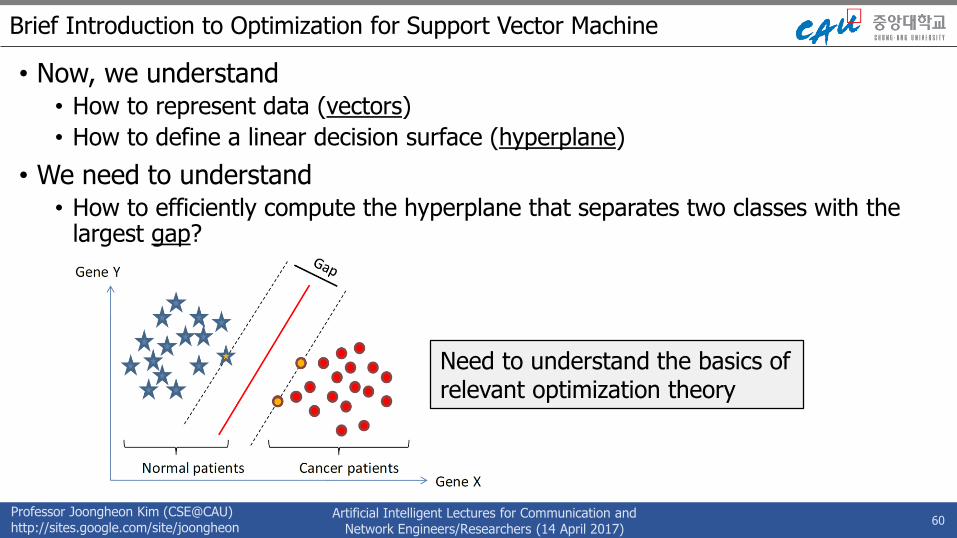
Brief Introduction to Optimization for Support Vector Machine

• Now, we understand• How to represent data (vectors)

• How to define a linear decision surface (hyperplane)

• We need to understand• How to efficiently compute the hyperplane that separates two classes with the

largest gap?

60

Need to understand the basics of relevant optimization theory




• Convex Functions• A function is called convex if the function lies below the straight line segment

connecting two points, for any two points in the interval.

• Property: Any local minimum is a global minimum.

61




• Quadratic programming (QP)• Quadratic programming (QP) is a special optimization problem: the function to

optimize (objective) is quadratic, subject to linear constraints.

• Convex QP problems have convex objective functions.

• These problems can be solved easily and efficiently by greedy algorithms (because every local minimum is a global minimum).

62




• Quadratic programming (QP)• [Example]

63

Consider 𝑥 = 𝑥1, 𝑥2

Minimize 1

2 𝑥 22 subject to 𝑥1 + 𝑥2 − 1 ≥ 0

Quadratic Objective Linear Constraints

Consider 𝑥 = 𝑥1, 𝑥2

Minimize 1

2𝑥12 + 𝑥2

2 subject to 𝑥1 + 𝑥2 − 1 ≥ 0

Quadratic Objective Linear Constraints



Outline

• Main Idea




64



SVM for Classification

• SVM for Classification• (Case 1) Linearly Separable Data; Hard-Margin Linear SVM

• (Case 2) Not Linearly Separable Data; Soft-Margin Linear SVM

• (Case 3) Not Linearly Separable Data; Kernel Trick

65




• (Case 1) Linearly Separable Data; Hard-Margin Linear SVM

66

• Want to find a classifier (hyperplane) to separate negative instances from the positive ones.

• An infinite number of such hyperplanes exist.

• SVMs finds the hyperplane that maximizes the gap between data points on the boundaries (so-called support vectors).

• If the points on the boundaries are not informative (e.g., due to noise), SVMs will not do well.





67

• The gap is distance between two parallel hyperplanes:𝑤 ∙ 𝑥 + 𝑏 = −1 and 𝑤 ∙ 𝑥 + 𝑏 = +1

• Now, we know that

𝐷 =𝑏1−𝑏2

𝑤, i.e., 𝐷 =

2

𝑤.

• Since we have to maximize the gap, we have to minimize 𝑤 .

• Or equivalently, we have to minimize 1

2𝑤 2.





68

• In addition, we need to impose constrains that all instances are correctly classified. In our case, 𝑤 ∙ 𝑥𝑖 + 𝑏 ≤ −1 if 𝑦𝑖 = −1𝑤 ∙ 𝑥𝑖 + 𝑏 ≥ +1 if 𝑦𝑖 = +1., i.e.,equivalently, 𝑦𝑖 𝑤 ∙ 𝑥𝑖 + 𝑏 ≥ 1.

In summary,

• Minimize 1

2𝑤 2 subject to

𝑦𝑖 𝑤 ∙ 𝑥𝑖 + 𝑏 ≥ 1, for 𝑖 = 1,⋯ , 𝑁




• (Case 2) Not Linearly Separable Data; Soft-Margin Linear SVM

69

• What if the data is not linearly separable? E.g., there are outliers or noisy measurements, or the data is slightly non-linear.

Approach• Assign a slack variable to each instance 𝜉𝑖 ≥ 0,

which can be thought of distance from the separating hyperplane if an instance is misclassified and 0 otherwise.

• Minimize 1

2𝑤 2 + 𝐶 𝑖=1

𝑁 𝜉𝑖 subject to

𝑦𝑖 𝑤 ∙ 𝑥𝑖 + 𝑏 ≥ 1 − 𝜉𝑖, for 𝑖 = 1,⋯ ,𝑁




• (Case 3) Not Linearly Separable Data; Kernel Trick

70

Data is not linearly separable in the input space

Data is linearly separable in the feature space obtained by a kernel



Questions?

71

Date post:	26-Aug-2018
Category:	Documents
Upload:	truongque
View:	223 times
Download:	0 times

Hidden Markov Models (HMM) and Probabilistic Graphical Models...

Documents